the Creative Commons Attribution 4.0 License.
the Creative Commons Attribution 4.0 License.
 | 18 Feb 2022
Air Control Toolbox (ACT_v1.0): a flexible surrogate model to explore mitigation scenarios in air quality forecasts
Augustin Colette
Laurence Rouïl
Frédérik Meleux
Vincent Lemaire
Blandine Raux
We introduce the first toolbox that allows exploring the benefit of air pollution mitigation scenarios in the every-day air quality forecasts through a web interface. Chemistry-transport models (CTMs) are required to forecast air pollution episodes and assess the benefit that shall be expected from mitigation strategies. However, their complexity prohibits offering a high level of flexibility in the tested emission reductions. The Air Control Toolbox (ACT) introduces an innovative automated calibration method to cope with this limitation. It consists of a surrogate model trained on a limited set of sensitivity scenarios to allow exploring any combination of mitigation measures. As such, we take the best of the physical and chemical complexity of CTMs, operated on high-performance computers for the every-day forecast, but we approximate a simplified response function that can be operated through a website to emulate the sensitivity of the atmospheric system to anthropogenic emission changes for a given day and location.
The numerical experimental plan to design the structure of the surrogate model is detailed by increasing level of complexity. The structure of the surrogate model ultimately selected is a quadrivariate polynomial of first order for residential heating emissions and second order for agriculture, industry and traffic emissions with three interaction terms. It is calibrated against 12 sensitivity CTM simulations, at each grid point and every day for PM10, PM2.5, O3 (both as daily mean and daily maximum) and NO2. The validation study demonstrates that we can keep relative errors below 2 % at 95 % of the grid points and days for all pollutants.
The selected approach makes ACT the first air quality surrogate model capable to capture non-linearities in atmospheric chemistry response. Existing air quality surrogate models generally rely on a linearity assumption over a given range of emission reductions, which often limits their applicability to annual indicators. Such a structure makes ACT especially relevant to understand the main drivers of air pollution episode analysis. This feature is a strong asset of this innovative tool which makes it also relevant for source apportionment and chemical regime analysis. This breakthrough was only possible by assuming uniform and constant emission reductions for the four targeted activity sectors. This version of the tool is therefore not suited to investigate short-term mitigation measures or spatially varying emission reductions.
- Article
(11855 KB) - Full-text XML
-
Supplement
(1675 KB) - BibTeX
- EndNote


The two most widespread applications of atmospheric chemistry modelling are (i) short-term air quality forecasting and (ii) long-term analysis of mitigation strategies. We introduce here the first toolbox able to address both issues at once, so that the user can explore the benefit of a long-term emission reduction control strategy for the present-day air quality forecast. Such a flexibility is provided by making the toolbox available through a web interface. The quality is ensured by relying on an emulator, or surrogate model, of the response of comprehensive air quality models to incremental emission reductions.
The development of atmospheric chemistry-transport models is motivated by the need to account for the dispersion and chemical evolution of pollutants in the atmosphere. A given influx of air pollutant emissions shall result in very different air concentrations depending on the meteorological conditions because of the dynamical and physical conditions (including advection, deposition, scavenging, turbulent mixing, etc.) and because of the chemical production and loss of secondary pollutants. As a result of this complexity of atmospheric chemistry and physics, there is no direct relationship between an incremental change of the emissions flux and resulting atmospheric concentrations.
Various approaches to air quality forecasting have been developed since the 1970s (Zhang et al., 2012). The first approaches relied on statistical regressions between observed air pollutant concentrations and various precursors (mainly meteorological variables). But such approaches faced structural limitations, chiefly in accounting for non-local air pollution brought about by long-range transport. Thus, 3-D chemistry-transport models are now widespread, for instance, in the European Air quality forecasts operated by the Copernicus Atmosphere Monitoring Services (Marécal et al., 2015; Engelen and Peuch, 2017).
Three-dimensional chemistry-transport models are also generally used to assess the benefit expected from a given air pollution control strategy (Colette et al., 2012). In that case, the computational burden increases because annual or multi-annual simulations are required. Such a burden constitutes a substantial limitation for the assessment of air pollution control strategies, where the end user is generally interested to compare the relative benefit of a series on individual mitigation measures. The replication of long-term chemistry-transport simulation for each mitigation strategy becomes then prohibitive.
That is why alternate techniques were developed for decision support applications by means of surrogate models that consist in simplified regressions fitted to the response of a comprehensive air quality model (Cohan and Napelenok, 2011; Amann et al., 2008; Pisoni et al., 2017). Such surrogate models generally rely on the assumption that the response to an incremental emission change can be approximated with a linear fit over a limited range of emission reduction magnitude. Such an approximation is required to limit the degrees of freedom of the surrogate model, especially when some geographical variability is accounted for in the surrogate model (i.e. when the emission reduction may vary in space, when exploring different magnitudes of emission reduction by country, for instance). The linearity assumption is also supported by limiting the scope of surrogate models to long-term indicators, such as annual mean exposure, which have a more linear response than short-term responses (Thunis et al., 2015).
In the present paper, we introduce a first surrogate response model (denoted the Air Control Toolbox (ACT) https://policy.atmosphere.copernicus.eu/CAMS_ACT.php, last access: 1 February 2022), which is able to capture the non-linear response of any magnitude of emission reduction for every-day air quality forecast. The model is designed to capture the daily means of both the PM10 and PM2.5 fractions of particulate pollution and nitrogen dioxide (NO2) as well as the daily mean and daily maximum of ozone (O, O). The spatial coverage is the greater European continent.
The overall objective is to offer the users a high degree of flexibility to explore any mitigation scenario through a web interface. We are targeting four activity sectors and for each of them the available emission reduction should cover the whole 0 % to 100 % range, for instance by 5 % increments. Using an explicit approach, this would imply 214 or 194 481 chemistry-transport simulations, which is obviously not feasible for computational reasons. The whole point of the present paper is therefore to design a methodology to reduce this number down to a reasonable number of simulations which can be performed on a daily basis and used as a training set to calibrate a simple response model.
The selected architecture of the response model is a polynomial function whose coefficients can be explicitly estimated from a limited number of simulations. Fitting more complex regression models could achieve better accuracy but only at the cost of a larger training set. We will see that a quadrivariate (four activity sectors) second-order polynomial can be well constrained with only a dozen of chemistry-transport simulations, which is quite acceptable with regards to the operational constrains of every-day production in an air quality forecasting system.
With this approach, all the complexity of the atmospheric chemistry response to incremental emission changes is embedded in a polynomial surrogate which is derived every day from on a subset of chemistry-transport simulations.
The use of a complete chemistry-transport model to build the training simulations allows accounting for all the important processes bearing upon the forecasted air quality, including long-range transport and chemistry. And the surrogate model is able capture some of the non-linearities existing between concentration and emission changes while remaining simple enough, in the sense that only a few coefficients need to be resolved.
The only two simplifications limiting the range of application of ACT are that emission reductions are assumed to apply (i) over the long term and (ii) over the whole modelling domain uniformly. ACT is therefore not suited to assess the benefit of emergency measures to mitigate air pollution episodes. It also not designed to assess the impact on long-term exposure to air pollution. The purpose of the tool is rather to assess the main activity sectors driving the day-to-day air pollution variability. Several diagnostics are proposed to achieve this by providing the source allocation and chemical regimes at various receptor locations, as well as mapping the benefit of reducing emissions over the whole modelling domain. If we take the analogy with climate change, the scope of ACT is analogous to attribution studies where one intends to quantify the role of climate change in the current meteorological situation, which is different than assessing the benefit of greenhouse gas strategies to mitigate long-term climate change.
Once the polynomial structure of the model is decided, an important part of the work consists in identifying the optimal set of those 10 to 15 chemistry-transport simulations that allow fitting a surrogate with adequate performance over any air quality situation. Most of the present paper is devoted to the description on how this numerical experiment plan is developed. The various methods (including overall surrogate structure, input data and the underlying air quality forecast system) are presented in Sect. 2, the step-by-step development and validation of the surrogate ACT model is introduced in Sect. 3. In Sect. 4, we present the web interface as well as a few case studies, and the use of the model in source allocation and chemical regime analysis is discussed in Sects. 5 and 6, respectively.
2.1 Testing periods
The ambition of the ACT surrogate model is to apply to the every-day air quality forecast. The surrogate model should therefore present satisfactory performance in any situation but especially during high air pollution episodes. For the development and validation purposes of the present article, we identified three case studies that are selected for their variety in terms of air pollution situation:
-
a case of intense cold spell with typical wintertime particulate matter pollution (December 2016–January 2017, Forêt et al., 2017);
-
a springtime PM episode dominated by ammonium nitrate formation (March 2015, Petit et al., 2017);
-
a summertime ozone episode (June 2017, Tarrason et al., 2017).
Note however that those periods do not constitute a specific training period for the surrogate model which is intended to be re-fitted to new chemistry-transport model (CTM) simulations every forecasted day in an automated calibration approach. Those episodes are only selected to identify the best design for the surrogate and assess its performance in reproducing the full CTM. We will see in Sect. 2.4 that in total 46 simulations were required to identify the optimum surrogate model structure and demonstrate its performance. All these 46 simulations covered the 4 months selected in the years 2015 to 2017 to capture a variety of air pollution episodes. But once the structure of the surrogate model is identified, the model itself is intended to be calibrated automatically on the basis of the day-to-day forecast.
2.2 Chemistry-transport model
The air quality simulations used for both the design of the numerical experiment and the every-day training of the ACT tool are performed with the CHIMERE chemistry-transport model (Mailler et al., 2017; Menut et al., 2013). The model is widely used for air quality research and application ranging from short-term forecasting (Marécal et al., 2015) to projection at a climate scale (Colette et al., 2015).
We use a simulation setup similar to the operational regional forecast performed under the Copernicus Atmosphere Monitoring Service (http://regional.atmosphere.copernicus.eu, last access: 1 February 2022), albeit with a lower spatial resolution: 0.25∘ instead of 0.1∘. The CHIMERE model version is CHIMERE2016a using Melchior gas-phase chemistry, a two-product organic aerosol scheme and ISORROPIA thermodynamics.
The anthropogenic emissions in the reference simulations are the Netherlands Organisation for Applied Scientific Research – Monitoring Atmospheric Composition and Climate (TNO-MACCIII) (Kuenen et al., 2014). Meteorological data are operational analyses of the IFS (Integrated Forecasting System) model of the European Centre for Medium-Range Weather Forecasts. The chemical boundary conditions are also obtained from ECMWF, as with the IFS model.
2.3 Surrogate model structure
The structure of the surrogate model is chosen to be a polynomial calibrated to 10 to 15 individual CHIMERE simulations performed every day for the air quality forecast extending between D+0 and D+2. The choice of a polynomial is for clarity and simplicity, and alternative parametric or non-parametric structures could be explored. The number of training scenarios (10 to 15) is constrained by the operational feasibility to perform multiple chemistry-transport simulations.
Four main activity sectors are desired to be captured by ACT, which correspond in terms of SNAP sectors (Selected Nomenclature for sources of Air Pollution) to the following:
-
AGR indicates agriculture (SNAP sector 10: including both crops and livestock);
-
IND indicates industry (SNAP sectors 1, 3, 4: combustion in energy and transformation industries, combustion in manufacturing industry, extraction and distribution of fossil fuels and geothermal energy);
-
RH indicates residential heating (SNAP sector 2: non-industrial combustion plants);
-
TRA indicates road transport (SNAP sector 7: urban and non-urban roads and motorways).
At present, the following sectors are therefore excluded from the tool, although they could be included in future versions: SNAP5 (extraction and distribution of fossil fuels and geothermal energy), SNAP6 (solvent and other product use), SNAP8 (off-road sources and machineries such as railways, shipping and air transport), SNAP9 (waste treatment and disposal).
Considering the goal to cover four activity sectors, and the operational constrain to compute only about 10 to 15 training scenarios every day, we can derive a limit in the number of coefficients which we can estimate. We conclude that the surrogate model can be at most a third-order polynomial or even less if interaction terms are accounted for.
It should be noted that the structure of the surrogate model ultimately developed is expected to deliver satisfactory performance for all pollutants (PM10, PM2.5, O, O and NO2). The final objective is to implement the surrogate model in an operational forecasting system with a continuous production, no matter whether the focus is on ozone or particulate matter episodes. Therefore, the selected structure required to deliver satisfactory performance for a given pollutant (e.g. a higher-degree polynomial, including interaction terms) can also yield indirect benefits for the other pollutants.
2.4 Emission reduction scenario available for development purposes
For development purposes, we performed an extensive set of CHIMERE simulations over the three air pollution episodes selected in Sect. 2.1 with various levels of emission reduction (10 %, 30 %, 60 %, 90 % and 100 %) for each of the four activity sectors (AGR, IND, RH, TRA). In all cases, emissions reductions are applied uniformly over Europe. It is also important to stress that all chemical species for a given activity sector are reduced by the same amount. This is different and complementary with the approach chosen for instance in the European Monitoring and Evaluation Programme (EMEP) source receptor matrices (Amann et al., 2008) or the SHERPA tool (Pisoni et al., 2017). In the remainder of the paper, those scenarios will be referenced by collating the sector and corresponding emission reduction magnitude, e.g. AGR60 for a 60 % reduction of agricultural emissions.
In addition to those emission reduction scenarios for individual sectors, we also explored interactions with scenarios where two sectors are reduced simultaneously. We included emission reductions of 30 %/60 % and 60 %/30 % for all pairs as well as 100 %/100 % reduction. Lastly, a 20 %/50 % reduction level was also included, so that in total we included 45 emission reduction scenarios in this design phase:
-
Reference
-
AGR10, TRA10, RH10, IND10
-
AGR30, TRA30, RH30, IND30
-
AGR60, TRA60, RH60, IND60
-
AGR90, TRA90, RH90, IND90
-
AGR100, TRA100, RH100, IND100
-
TRA20AGR50, TRA30AGR60, TRA60AGR30, TRA100AGR100
-
TRA20IND50, TRA30IND60, TRA60IND30, TRA100IND100
-
AGR20IND50, AGR30IND60, AGR60IND30, AGR100IND100
-
AGR20RH50, AGR30RH60, AGR60RH30, AGR100RH100
-
IND20RH50, IND30RH60, IND60RH30, IND100RH100
-
TRA20RH50, TRA30RH60, TRA60RH30, TRA100RH100
Here, we present the various steps towards building the polynomial surrogate model calibrated on an optimal set of training scenarios. The complexity of the model increases gradually from a univariate form to a multivariable non-linear polynomial including interactions. But to start with, the responses of air quality to a given emission reduction for various locations and episodes are illustrated.
3.1 Univariate sensitivity to emission reductions
3.1.1 Univariate air quality response at individual location
In this section, we present the sensitivity to emission changes for either PM10 or O3 in three target cities (Brussels, Paris and Milan) and for the three types of episodes. We aim to illustrate to what extent the air quality response is linear for each activity sector and species. At this stage, we only present the response in the complete air quality model (CHIMERE); the ability of a surrogate to reproduce this sensibility will be the focus of the following sections.
In Fig. 1, we show the difference, at a given point, between the PM10 concentration when reducing emission of a single activity sector and the concentrations in the reference simulation. Those differences can be computed from various levels of reduction: 0 % (reference), 10 %, 30 %, 60 %, 90 % and 100 %.
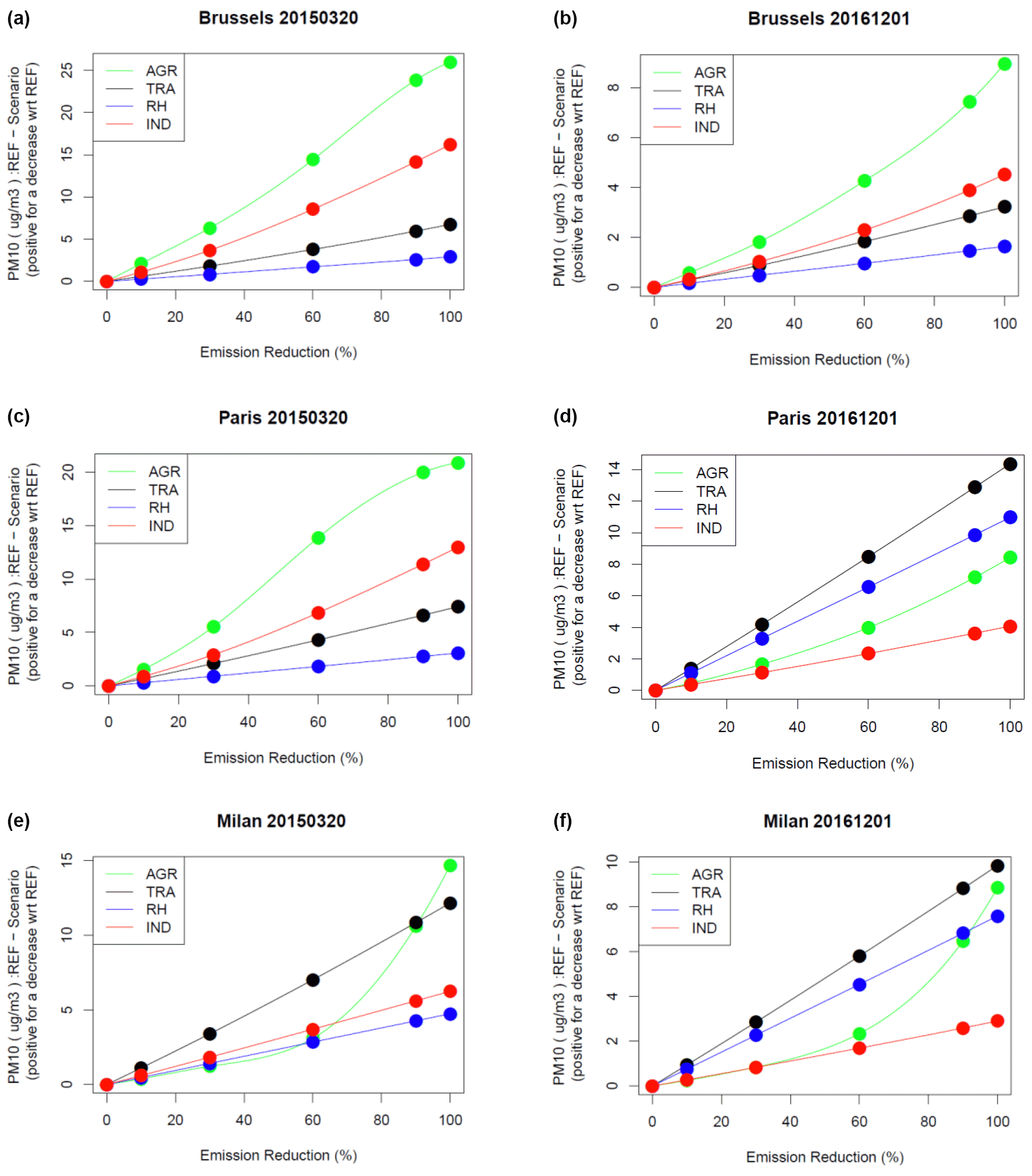
Figure 1Modelled PM10 reduction (y axis: positive for a decrease with respect to the reference, µg m−3) for a given reduction in agriculture (green), industrial (red), residential heating (blue) and traffic (black) emissions (x axis: in %) in Brussels, Paris and Milan and for 20 March 2015 (a, c, e) and 1 December 2016 (b, d, f).
The PM10 concentration response to incremental emission reductions depends on the date, location, and activity sector. The temporal and spatial sensitivity yield substantial complexity in air quality modelling. But we note here that the relationship to incremental emission changes can be relatively simple and well fitted by low-order polynomial or even linear relationships.
The residential heating (RH) sector contributes mainly with primary PM10 emissions or organic aerosol precursors, and its response is the closest to linearity for 20 March 2015 and 1 December 2016 and the three selected cities. It is also the case for the traffic (TRA) sector. But for industry (IND), and even more so for agriculture (AGR), there is a clear non-linear response. In most cases, such responses follow a second-order polynomial. It is for Milan that the steepness of the quadratic term is largest. And for the first episode (March 2015), which is the episode the most influenced by ammonium nitrate pollution, the shape is closer to a third-order polynomial for Brussels and Paris. Very similar behaviour is found for PM2.5, displayed in the Supplement (Fig. S1).
The ozone sensitivity to emission changes is illustrated in Fig. 2 for both ozone peaks and ozone daily average. As far as ozone peaks are concerned, a quadratic sensitivity is found for traffic and industrial sources, the main providers of NOx and VOC emissions. For the selected day (which is the peak of the episode), traffic is the main factor, although industry is sensitive also for Brussels. Note the negative contribution of agriculture which, by providing NH3, sequestrates a fraction of nitrogen oxides to form ammonium nitrate, leading indirectly to decrease ozone levels.
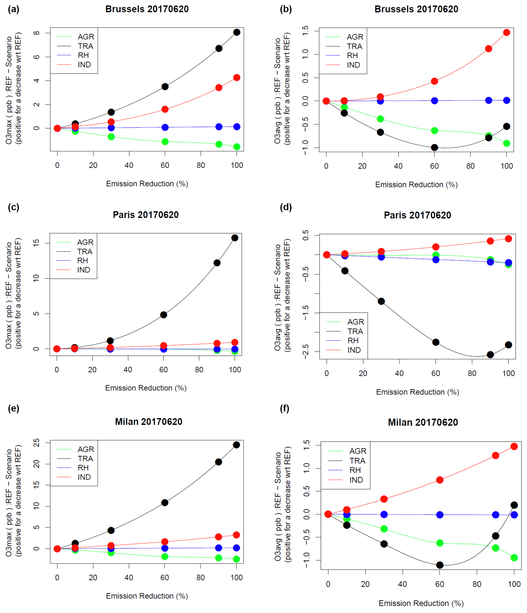
The sensitivity to the traffic sector is very different for ozone daily average because that sector is the main contributor to NOx emissions. The switch from high-NOx to low-NOx regimes can be clearly seen in all three cities in the sensitivity of daily average O3 when the emission reduction exceeds 60 % for the traffic sector. This very distinct sensitivity of O3 daily maximum and daily averages is due to the titration process, which affects more strongly nighttime low-ozone concentrations and is therefore less visible on the daily maximum. In Fig. 2, it is a specific feature of the traffic sector, which is not seen, for instance, for industrial emissions. It should be noted that the ratio is very different for both sectors. In the CHIMERE modelling setup used here, 20 % of NOx emissions are allocated to NO2 for the traffic sector, while for other sources including industry it is only 4.5 % of NOx emissions that are constituted of NO2. But this larger share of NOx emissions as NO in the industry sector would rather imply a lower titration of O3 by NO in traffic emissions compared to industrial sources. And in summer, NO and NO2 will even out very fast at the spatial scales of a regional chemistry-transport model. The stronger impact of titration when reducing traffic emissions in Fig. 2 is therefore rather a consequence of the overall larger share of total NOx emissions compared to other activity sectors. The corresponding figures for NO2 for both a wintertime (December 2016) and summertime (June 2017) episode are provided in the Supplement (Fig. S2), although the response is mostly linear.
3.1.2 Univariate model performance over Europe
Here, we investigate the selection of the optimal model independently for each activity sector; thus, we introduce four univariate models for the activity sectors: AGR, IND, RH, and TRA. The calibration is also performed for the four pollutants of interest: PM10, PM2.5, O, O, NO2.
For each day, and each pollutant, a polynomial model is calibrated at each grid point of the modelling domain. We introduce the following notations for a third-order polynomial, with αi,j, βi,j, γi,j the coefficients (the later two being nullified for linear or quadratic forms):
where
-
is the air pollutant concentration (for either PM10, PM2.5, O, O or NO2) modelled with the CTM for the reference simulation with emissions εref.
-
Ci,j is the air pollutant concentration modelled with the CTM for the sensitivity simulation with reduced emissions for sector “sec”: εsec reduced by a uniform factor δsec over the domain. In addition to being uniform in space, the reduction factor is also identical for all emitted precursor species since it is applied to the whole activity sector.
-
Throughout the paper, the coefficients α, β and γ of such polynomials will be computed for each i,j pair of latitude, longitude indices in the geographical modelling domain, so the indices will be dropped in the following notations.
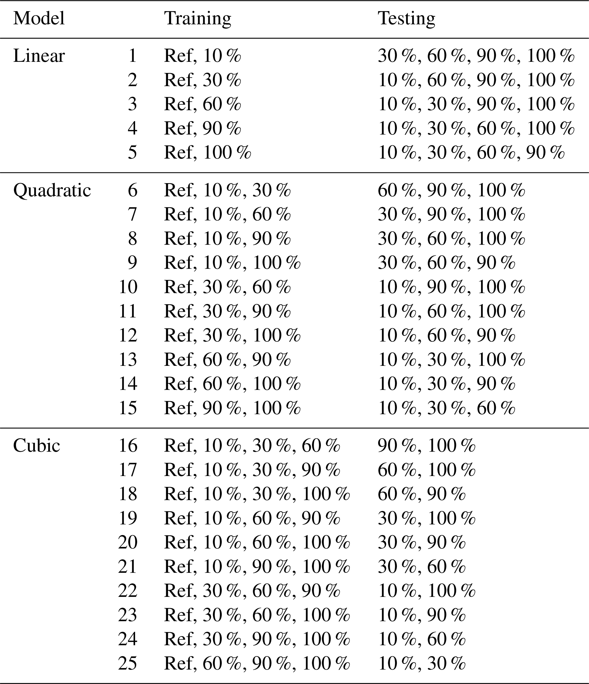
Depending on the model complexity (linear, quadratic or cubic), the model is calibrated with one, two or three sensitivity simulations (in addition to the reference). The pairs involving the 0 % reduction and any of the other amount of reduction allow computing a linear polynomial. Triplets involving the 0 % reduction and any combination of two other reductions are used to compute a quadratic polynomial. And an analogous quadruplet is used for cubic polynomials. Then the model is tested by computing the error of its prediction with respect to the remaining available sensitivity simulations that were not used in the calibration. For the purpose of model development, we performed sensitivity simulations over the three selected case studies with uniform reductions of the emissions for AGR, IND, TRA and RH by 10 %, 30 %, 60 %, 90 % and 100 %. The corresponding list of scenarios available for training and testing is summarized in Table 1; there are 5, 10 and 10 combinations for the linear, quadratic and cubic forms, respectively.
Table 1List of CTM sensitivity simulations used to train and test the various linear, quadratic and cubic forms of the surrogate model.
The error that we discuss here is the absolute difference between the concentration change predicted with the surrogate model for a given emission reduction () and the corresponding validation CHIMERE simulation (C−Cref) for the same emission reduction (δsec). Each polynomial model can be tested against several independent CHIMERE validation simulations (4, 3 and 2, for linear, quadratic and cubic forms, respectively), so that an average of absolute errors is taken (). We also include a relative error, where a normalization by the corresponding pollutant concentration is used ().
The errors of the models are computed for each day and grid point, allowing a discussion of the surrogate performance both in terms of spatial and temporal variability.
Figure 3 shows the day-to-day variation of the absolute and relative errors of the various univariate PM10 models for the agriculture sector, averaged for all grid points in the region 40 to 55∘ N and 10∘ W to 30∘ E. The time period displayed here spans from 30 November 2016 to 29 December 2016 and includes two important air pollution episodes around 8 and 20 December 2016. The models are listed in the same order as in Table 1 with first the 5 linear models, then the 10 quadratic and 10 cubic forms.
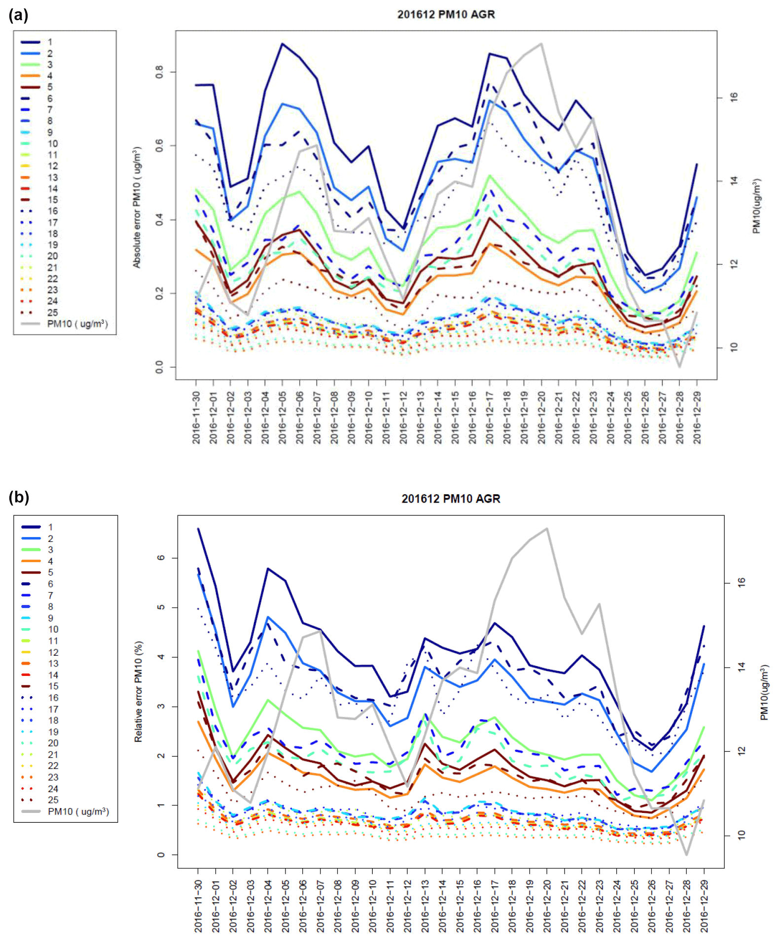
Figure 3Absolute (a, µg m−3) and relative (b, %) error over western Europe of the univariate surrogate model for the agriculture activity sector in December 2016. The coloured lines are for individual polynomial surrogate models and training scenarios (x axis: 5 linear, 10 quadratic and 10 cubic forms with indices of the x axis matching the rows of Table 1). The grey curve gives the day-to-day variation of PM10 (µg m−3) averaged over the region (displayed on the right-hand-side y axis).
The first five surrogate models with solid lines and blue colours have a linear structure. They have larger errors than the following more complex models, with relative errors ranging from 1.4 % to 4 %. The worst linear model is computed with the 10 % emission reduction scenario (and the reference), whereas the linear model computed with the 90 % emission reduction scenario is performing better than several more complex models.
Moving to a second-order polynomial improves notably the performance. In total, 10 combinations of training scenarios (and the reference) are available to compute a quadratic polynomial. For each of them, three validation scenarios are available to assess the performance. The best quadratic model for that time period relies on the 60 % and 100 % emission reductions, its relative error is lower than 0.1 µg m−3 or 0.65 %. Note that the quadratic models using training scenarios confined within a narrow range of emission reductions (e.g. 10 % and 30 %, or 90 % and 100 %) do not perform well, even when compared to the simple linear polynomial.
The third-order polynomial performs best, except the last model which uses only the largest emission reduction and is therefore too weakly constrained for the lower range of reductions. The smallest error for a cubic model is 0.05 µg m−3 or 0.37 %.
At this stage, it becomes clear that a trade-off must be sought between model performance and complexity considering that moving from a second- to third-order polynomial requires computing one more training scenario, whereas the error of the quadratic polynomial is already below 1 %.
The errors presented in Fig. 3 are an average over a large fraction of Europe. To check if they do not hide some compensations between different regions, we also show in the map of relative errors, averaged over the whole month of December 2016 (Fig. 4). The quadratic model performing best according to Fig. 3 is calibrated to 60 % and 100 % emission reductions. The map of error shows that the largest errors are found over the Po Valley, but it is also the case of all the other quadratic models represented in the figure. Therefore, we conclude that the selection of the best-performing model done on the basis of average performance in Fig. 3 does not include compensation between different regions.

Figure 4Relative error (%) averaged over the month of December 2016 for the quadratic univariate PM10 models with respect to the agriculture activity sector. The sensitivity scenarios used to train the individual models are indicated in the title of each panel, as well as the average error.
A similar analysis is performed for the other activity sectors; the analogues of Fig. 3 for traffic, residential heating and industry are provided in the Supplement (Figs. S3 to S8).
The performance of the univariate model is presented in Fig. 5 for PM10. The four activity sectors are still treated independently at this stage; the interactions and performance of multivariate models will be discussed in Sect. 3.2 and 3.3, respectively. Instead of showing the average error in space or time as in Figs. 3 and 4, respectively, we show here the whole distribution of error for any grid point in western Europe, and any day over three 1-month particulate matter air pollution episodes (March 2015, December 2016 and January 2017). The main features of those distributions are given as box plots with the boxes providing the first quartile, median and third quartile. Whiskers extend to 1.5 times the interquartile range from the borders of the box, and the extreme points lying outside of that range are also provided. As in Fig. 3 and Table 1, we show (from left to right) first the five linear surrogate models, and then the 10 quadratic and 10 cubic forms. The numerical values of the median of those distributions are given in the Supplement (Table S1).
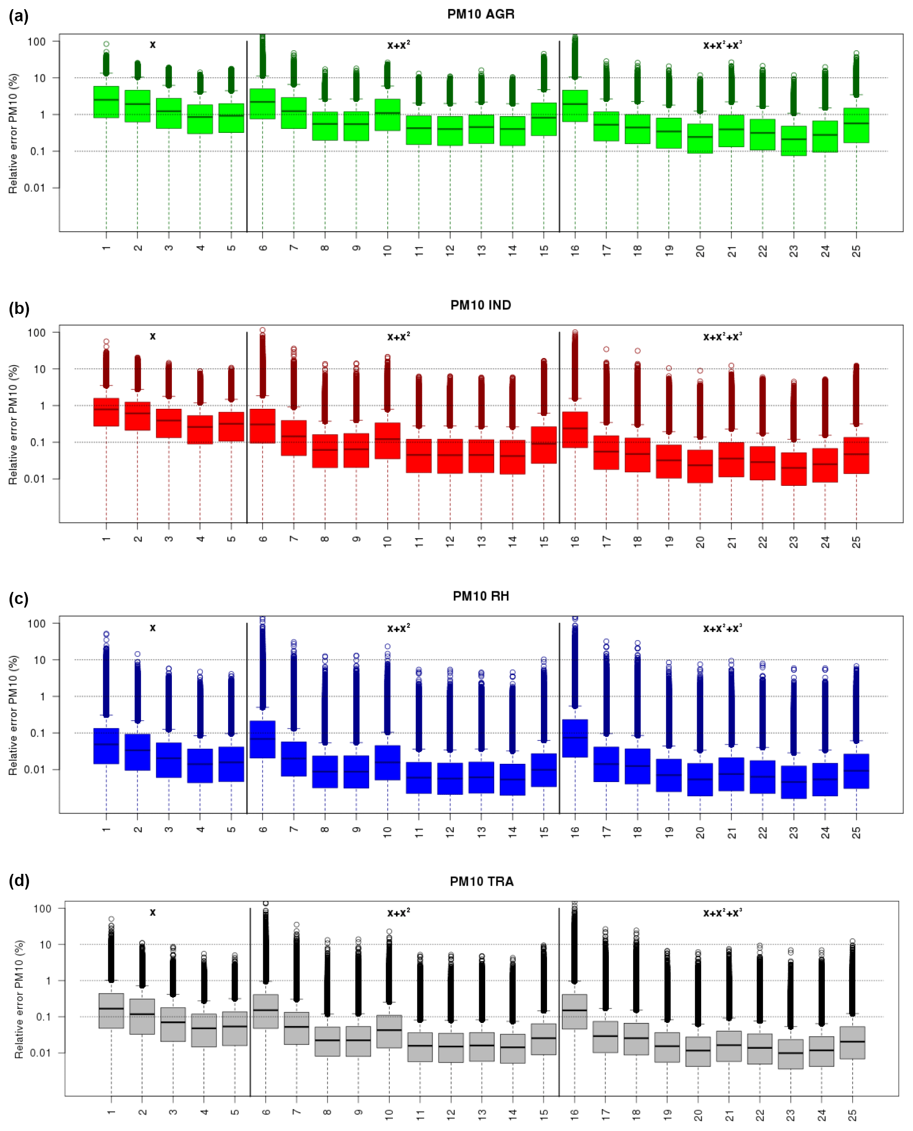
Figure 5Relative error (%) of the PM10 univariate surrogate models for either AGR, IND, RH, TRA (a–d) and for various polynomial forms and training scenarios (x axis: 5 linear, 10 quadratic and 10 cubic forms with indices of the x axis matching the rows of Table 1). The box plots indicate the minimum, first quartile, median, third quartile and maximum in the distribution of relative errors at each grid point in western Europe and each day over three air pollution events (March 2015, December 2016, January 2017). The horizontal dotted lines are for 0.1 %, 1 % and 10 % errors.
For each activity sector, we find in general that the linear models do not perform as well as the quadratic or cubic polynomials. But for some activity sectors, the linear model can be considered satisfactory.
It is the case for the residential heating sector, where a linear model relying on the scenario with 90 % reduction (index 4 in the x axis of Fig. 5) is already very good: the upper 95 % confidence interval is lower than 0.1 %. The median of relative errors is then 0.03 % (Table S1) and the gain when moving to a quadratic form is only a factor of 2.
On the contrary, for industry and traffic, we opt for a quadratic model (using 60 % and 100 % reductions, index 14 in the x axis of Fig. 5) which yields median errors below 0.1 % (0.099 % and 0.028 % for IND and TRA, respectively) and the gain in term of median error is a factor of 3–4 compared to the linear forms. For the selected quadratic form and 60 % and 100 % reduction training scenarios, we can ensure that the relative error of the surrogate model is below 10 % for any day and any grid point and even below 0.1 % for 75 % of the points in the distribution.
For the impact of the agricultural sector on PM10, the non-linearity is such that we have to lower slightly the ambition on the performance of the surrogate. Nevertheless, by selecting a quadratic form trained on the scenario with 60 % and 100 % reduction (index 14 in the x axis of Fig. 5), we can still ensure that the relative error does not exceed 10 % for any day and grid point, and even remains below than 1 % for 75 % of the points in the distribution.
The choice to select a quadratic model for industry and traffic is further supported by the analysis for ozone (Fig. 6, and corresponding numerical values in Table S2 in the Supplement), where a clear improvement is found compared to linear forms. Selecting a quadratic model trained on 60 % and 100 % emission reduction scenarios allows reaching relative errors lower than 10 % for any day and any grid point, and 95 % confidence interval lower than 0.1 %.
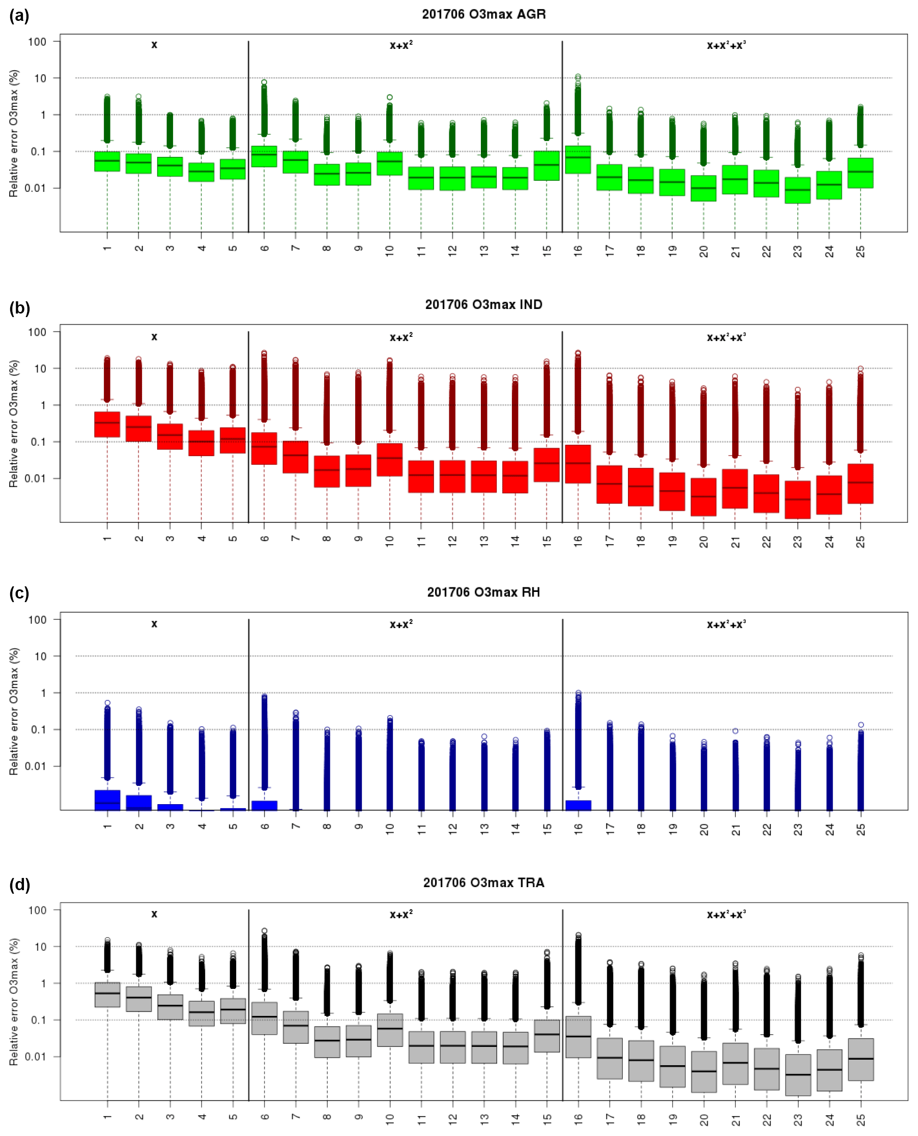
A linear model could be fit for purpose with regards to ozone sensitivity to agriculture emissions, but since a quadratic form was selected for PM10, it will also benefit the ozone models. For residential heating, most errors are below 0.001 % so that the ozone result only confirms the satisfactory behaviour of the linear model.
3.2 Bivariate models and interactions
After having introduced quadratic terms, we investigate cross-sector interactions. First, we assess the need of whether or not to account for interaction terms. In the case where the added value of interaction terms is demonstrated, we identify the optimal training scenarios.
The surrogate models that we use here are bivariate, second-order polynomials, plus an interaction term; quadrivariate models will be discussed in Sect. 3.3. For instance, for the bivariate model of agriculture and industry, we have the following structure:
In order to assess the need to account for interactions, we only use training scenarios with 30 % and 60 % reduction levels.
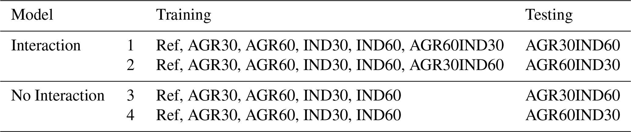
First a bivariate quadratic model without interactions is trained with the 30 % and 60 % reduction levels and tested against corresponding interaction scenarios. Taking the example of agriculture and industry, we would have the two training and testing configurations in lines 3 and 4 of Table 2.
Table 2List of CTM sensitivity simulations used to train and test the need to account for interactions in the quadratic forms of the surrogate model.
The box plots of Fig. 7 display the performance when including (first two box plots of each panel) or excluding (last two box plots) interaction terms. The numeric values of the median of these distributions are available in Tables S3 and S4 of the Supplement. As could be expected given the relatively linear behaviour of the response to residential heating emission changes, interactions do not bring substantial added value for those terms: (AGR, RH), (IND, RH), (TRA, RH). On the contrary, keeping 75 % of the points and days with a relative error lower than 1 % requires us to account for interactions for the pairs (AGR, IND) and (TRA, AGR).

Figure 7Relative error (%) of the PM10 bivariate surrogate models (a–f: AI: AGR and IND, AR: AGR and RH, IR: IND and RH, TA: TRA and AGR, TI: TRA and IND, TR: TRA and RH). For each panel, the box plots of the distribution of errors are given for two models with interactions (a, d) and two models without interactions (c, f), where indices in the x axis match the row of Table 2. The distributions of relative errors include each grid point in western Europe and each day over three air pollution events (March 2015, December 2016, January 2017). The horizontal dotted lines are for 0.1 %, 1 % and 10 % errors.
For ozone (Fig. 8 and Table S4 of the Supplement), the only important interaction terms are for the (TRA, IND) pair of sectors, which was expected since those bring the largest share of ozone precursor emissions. When ignoring their interactions, the upper 95th confidence interval of relative error distribution can reach 1 %, whereas it remains below 0.1 % when interactions are taken into account.

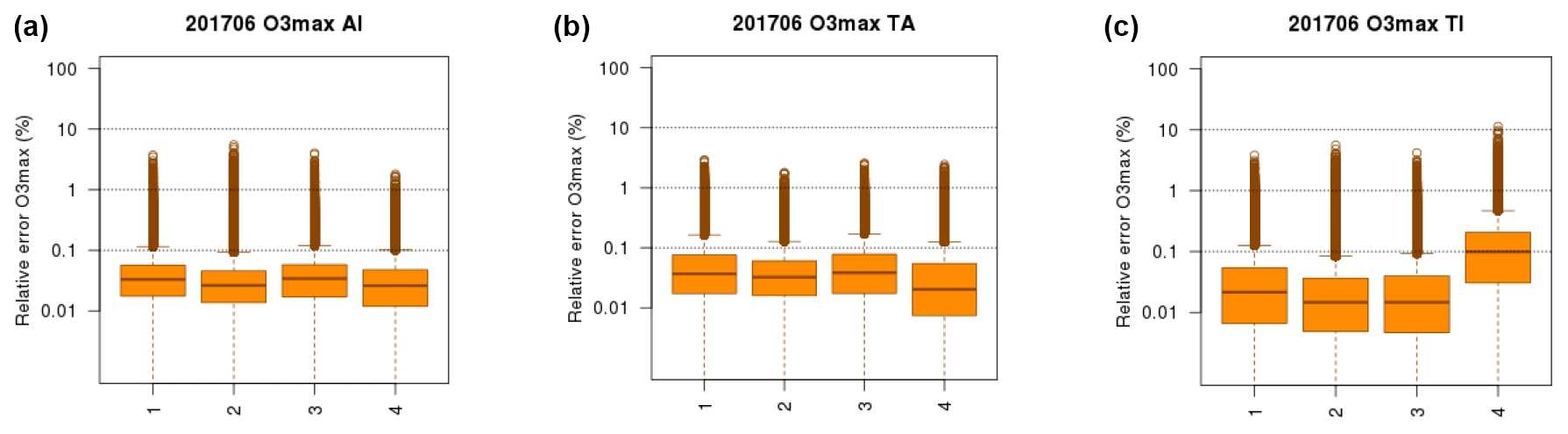
For the pairs where interactions must be taken into account – (AGR, IND), (TRA, IND) and (TRA, AGR) – we remain to identify the optimal level of reduction in the training scenario. We set the range of reduction identified in Sect. 3.1.2 for the quadratic terms (60 %/100 %) and seek to identify the optimal reduction for the scenario designed to capture interaction terms. The list of available combinations to train and test each interaction term is given in Table 3.
Table 3List of CTM sensitivity simulations used to select the optimal scenario by training and testing the various combinations to account for interactions in the quadratic forms of the surrogate model.
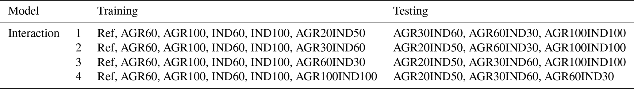
The 30 %/60 % reductions are optimal for the (AGR, IND) and (TRA, IND) pairs, but for the (TRA, AGR) pair, better performance is found with a interaction term. The same feature is found for both PM10 and O, as seen in Figs. 9 and 10, and corresponding numerical values in Tables S5 and S6 of the Supplement.

Figure 9Relative error (%) of the PM10 bivariate surrogate models (a–c: AI: AGR and IND, TA: TRA and AGR, TI: TRA and IND). For each panel, the box plots of the distribution of errors are given for four models with interactions trained on different scenarios where indices in the x axis match the row of Tables 3 and 2. The distributions of relative errors include each grid point in western Europe and each day over three air pollution events (March 2015, December 2016, January 2017). The horizontal dotted lines are for 0.1 %, 1 % and 10 % errors.
3.3 Quadrivariate models and interactions
The methodology followed in Sect. 3.1 and 3.2 consists in selecting first the optimal structure for univariate models, before investigating bivariate models including interactions terms. Such a step-by-step approach allows a clear introduction of the methodology. This presentation has a clear pedagogical advantage. It is also relevant for a potential development of a similar approach in a different context. One could consider developing an ACT tool over a different region or at higher spatial resolution. But, in that case, nothing guarantees that the same model structure would be selected, in particular if non-linearities affect different activity sectors.
However, such a sequential approach carries a risk of not selecting the optimal structure, as pointed out for stepwise regression approaches. Indeed, with a sequential method, we assume that the optimal structure and training scenario remains valid when including interactions whereas there is a possibility that the addition of an interaction term could change the selection of univariate terms.
Therefore, we investigated directly a four-dimensional model with the following structure:
Such a model requires two training scenarios for AGR, IND, TRA, one for RH and one for each of the three interaction terms. With this approach, all possible two-term interactions are indeed taken into account as only those involving RH are excluded because we have demonstrated earlier that this factor could be well approximated with a linear relationship (and therefore irrelevant for second-order interactions).
We did not investigate all possible of the 46 available testing scenarios but a subset applying the same range of reduction for each of the univariate component (i.e., for instance, only AGR30, AGR60, IND30, IND60, RH30, TRA30, TRA60) and complementary reduction for the interaction terms (not using 30 %/60 % reductions for our example). With these constrains, we are still left with an impressive number of 285 combinations. The performance (as median relative error) of the optimal set of training scenarios identified in Sect. 3.1 and 3.2 is confirmed here as it ranks respectively 21st, 4th and 7th for the PM10 episodes of March 2015, December 2016, January 2017. Other combinations of training scenarios can indeed be identified for given episodes, but the choice we propose is also robust across various episodes and always within 5 % of the errors of the optimal model. For ozone daily maximum, the model with the step-by-step methodology beats any of the other 285 configurations.
To summarize, the model that we selected is a quadrivariate polynomial, first order for RH emissions and quadratic for AGR, IND and TRA, with interaction terms for the pairs: (AGR, IND), (TRA, IND) and (TRA, AGR). The optimal set of training scenarios include the 10 sensitivity simulations selected above, to which a reference is added as well as a simulation where the emissions of sectors are reduced by 100 % to ensure that the model remains bounded:
-
Reference
-
AGR60, AGR100
-
IND60, IND100
-
RH90
-
TRA60, TRA100
-
AGR30IND60
-
TRA30IND60
-
TRA100AGR100
-
AGR100IND100RH100TRA100
This final model is tested against the 34 available scenarios not used in the training. We conclude that with such a model structure and training scenarios, it is possible to reach the surrogate model performance summarized in Fig. 11 that shows that relative errors are below 1 % at 75 % of the grid points and days, below 2 % at 95 % of the grid points and days, and below 10 % for any grid points and days. More specifically, the single highest error over the 864 248 grid points and days considered is 7.5 %, 7.9 %, 4.8 %, 2.8 % and 2.9 % for PM10, PM2.5, NO2, O and O.
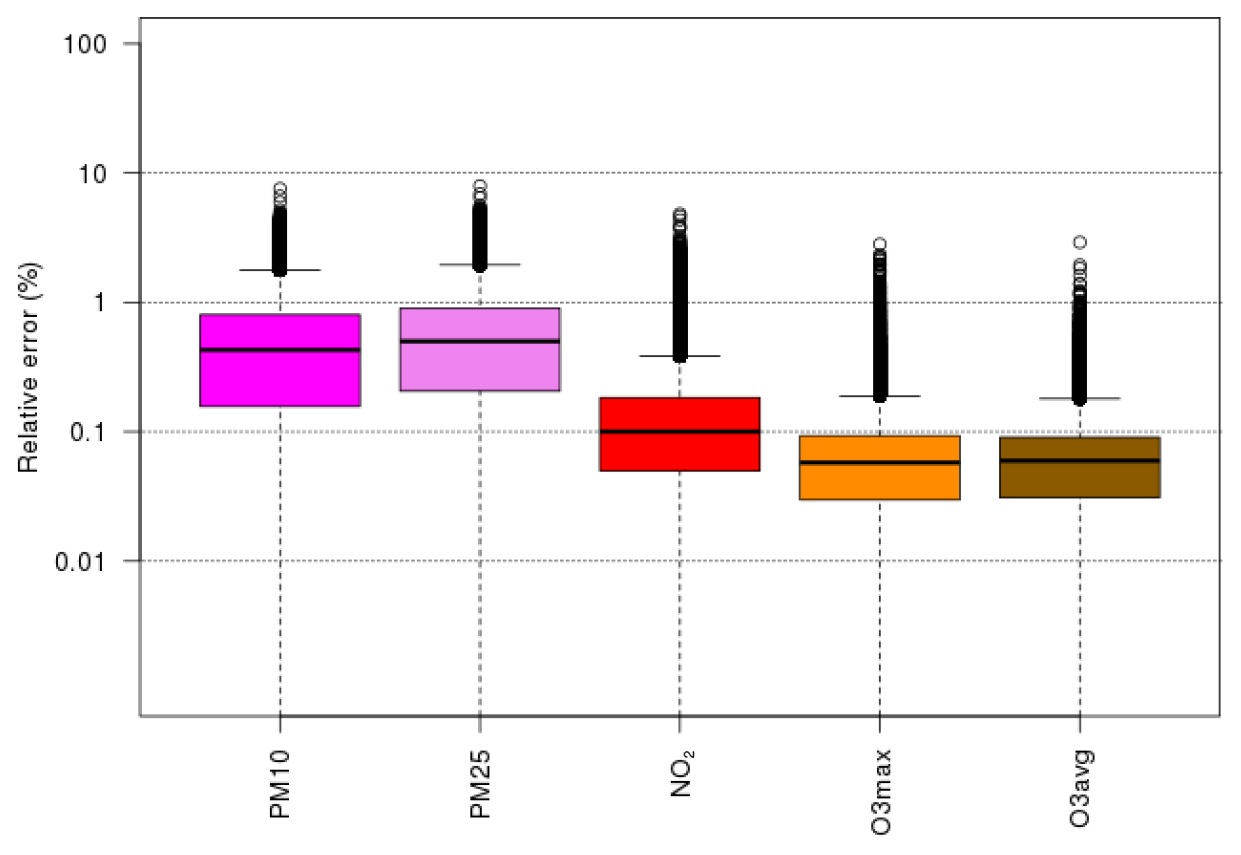
Figure 11Relative error of the final selected surrogate model for all pollutants. The box plots represent the distribution of relative errors over each grid point in western Europe and each day during the relevant air pollution events: wintertime (March 2015, December 2016, January 2017) for PM10, PM2.5 and NO2, summertime (June 2017) for O (i.e. daily maximum ozone) and O (daily average).
This structure is selected because of its good performance for all relevant ambient air pollutant as demonstrated here over a range of air pollution episodes. In the operational model, the overall structure of the model is frozen, while only the coefficients of the surrogate are recomputed every day on the basis of the current air quality forecast. It should be noted however that any evolution of the model such as increasing the spatial resolution, implementation over a different geographic area or including other activity sector would require revising this structure.
Further increasing the degree of the polynomial would certainly improve the quality of the surrogate model. The only two reasons not to engage in that direction are (i) to avoid increasing the computation burden with more training scenarios and (ii) when considering that the performance achieved at order 2 is already very satisfactory. The only higher-order interaction scenario removing emissions from all four sectors is designed as a closure to avoid any potential negative concentrations.
5.1 Description of ACT interface
The routine production of ACT relies on two main steps. First the 12 training scenarios corresponding to the current air quality forecast are simulated on a high-performance computer with the CHIMERE model with a setup inspired from the French Air Quality Platform Prev'Air (Rouïl et al., 2009) and the European CAMS regional production (Marécal et al., 2015). Then the surrogate model is automatically calibrated and exported to a web interface using the shiny package of the R language.
An annotated screenshot of the ACT web interface is given in Fig. S9 of the Supplement. First, the pollutant of interest is selected in the list of compounds for which the surrogate has been validated: PM10, PM2.5, NO2, O and O, all of which are daily mean values, except for O which is the daily maximum level. The base time of the forecast can also be changed up with access to a long history as well as its valid time.
A series of slide bars allow the user to define its tailored scenario, reducing by any percentage the emission originating from road transportation, industry, residential heating and agriculture. Considering that there are also other sources of pollution than those included in ACT (i.e. AGR, IND, RH and TRA), a possibility to include or remove those other contributions is offered in order to visualize a reference simulation including only the sources upon which the user can interact through the slide bars. Such “other contributions” include mainly natural emissions (e.g. dust and sea salt for particulate matter, or biogenic VOCs) but also some activity sectors not included at present in the tool (e.g. international shipping). It is computed by withdrawing from the CHIMERE reference simulation a scenario emulated with ACT with all four activity sectors set to zero. As a consequence, the tropospheric ozone burden is also withdrawn; that is why the corresponding menu refers to “natural and background concentrations”.
The results are then displayed as a map for either the selected scenario or the difference compared to the reference simulation.
5.2 Case studies of scenario analysis
The use of the ACT interface is illustrated here, taking as example the training episodes introduced in Sect. 2.1.
5.2.1 March 2015
In March 2015, a remarkable PM10 episode spread throughout a large part of western Europe for almost a week. The daily mean for 18 March 2015 displayed in Fig. 12 is given either with all sources included (left) or only for the sources included in ACT: AGR, IND, RH, TRA (so that in that panel natural and background concentrations are excluded). As explained in Sect. 4.1, the other sources are mainly natural (desert dust and sea salt), but they also include some activity sectors not available in ACT (such as international shipping).
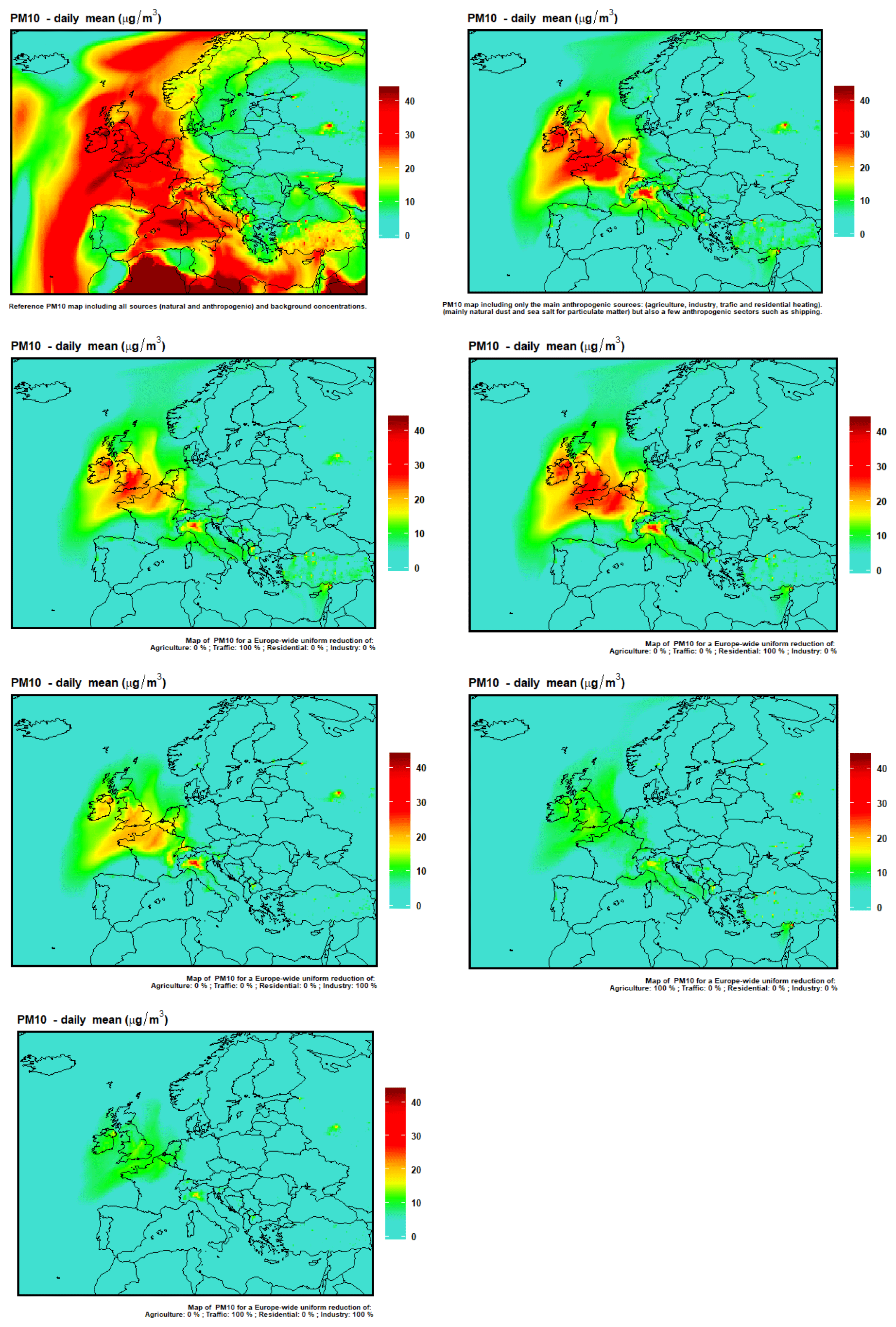
Figure 12First row: PM10 concentrations on 18 March 2015 including (left) or excluding (right) natural and background concentrations. Following rows: PM10 daily average concentrations emulated with ACT for 18 March 2015 for a 100 % reduction of traffic emissions (second row, left), residential emissions (second row, right), industry emissions (third row, left), agriculture emissions (third row, right) and both traffic and industry (fourth row, right).
During that episode, the PM10 composition was dominated by inorganic aerosols (Petit et al., 2017), and more specifically ammonium nitrate, which is formed by chemical reactions between ammonia and nitrogen oxides emitted by any combustion sources (traffic or other). In Europe, 93 % of annual NH3 emissions were due to agriculture in 2015 (according to EMEP emissions for EU28 available at https://www.ceip.at, last access: 1 February 2022), about half of which were due to livestock and the other half to fertilizer. Fertilizer spreading is a very seasonal activity that dominates in March. Because NH3 resulting from fertilizer spreading is emitted over very large areas, and because of the lifetime of fine PM in the atmosphere, the resulting air pollution plume can reach a substantial geographical extent as we can see here with high PM10 levels modelled far out over the Atlantic Ocean. This type of air pollution event is a textbook example of the regional character of atmospheric air pollution.
In order to illustrate the capacities of the ACT tool, four scenarios are emulated by removing independently 100 % of the emission of each of the four main activity sectors (Fig. 12). These scenarios are all emulated on the basis of the simulation excluding natural sources, i.e. to be compared to the top-right panel of Fig. 12.
The reduction of agricultural emissions has the largest effect on PM10 concentrations and only a couple of hotspots remain, for instance, in the Po Valley. On the contrary, none of the scenarios where only one of the other sectors is reduced manages to reach low PM10 levels. This is because NH3 remains in excess and removing all the NOx from traffic has little effect if the NOx from industry and residential heating remains available. We can note however that the punctual sources in Turkey or Ukraine disappear in the scenario where industrial emissions are set to zero. Lastly, industrial emissions have a larger effect on regional pollution than traffic, which seems contradictory to the high attention given to road transportation during major air pollution episodes.
Lastly, we also display an emulated scenario where both traffic and industrial emissions are set to zero, whereas agriculture emission are unchanged. Here, we obtain low PM10 levels similar to the no-agriculture scenario because most sulfur and nitrogen oxides are removed.
5.2.2 December 2016
In December 2016, a large particulate matter episode developed in western Europe under the influence of cold and stable meteorological conditions that kept air pollutants near the ground in the inversion layer (Forêt et al., 2017). In addition, cold temperatures induced an increase in residential heating emission. The reference simulation for daily mean PM10 on 1 December 2016 is presented in Fig. 13. It only includes the sources of the main activity sectors (e.g. excluding natural and background concentrations).
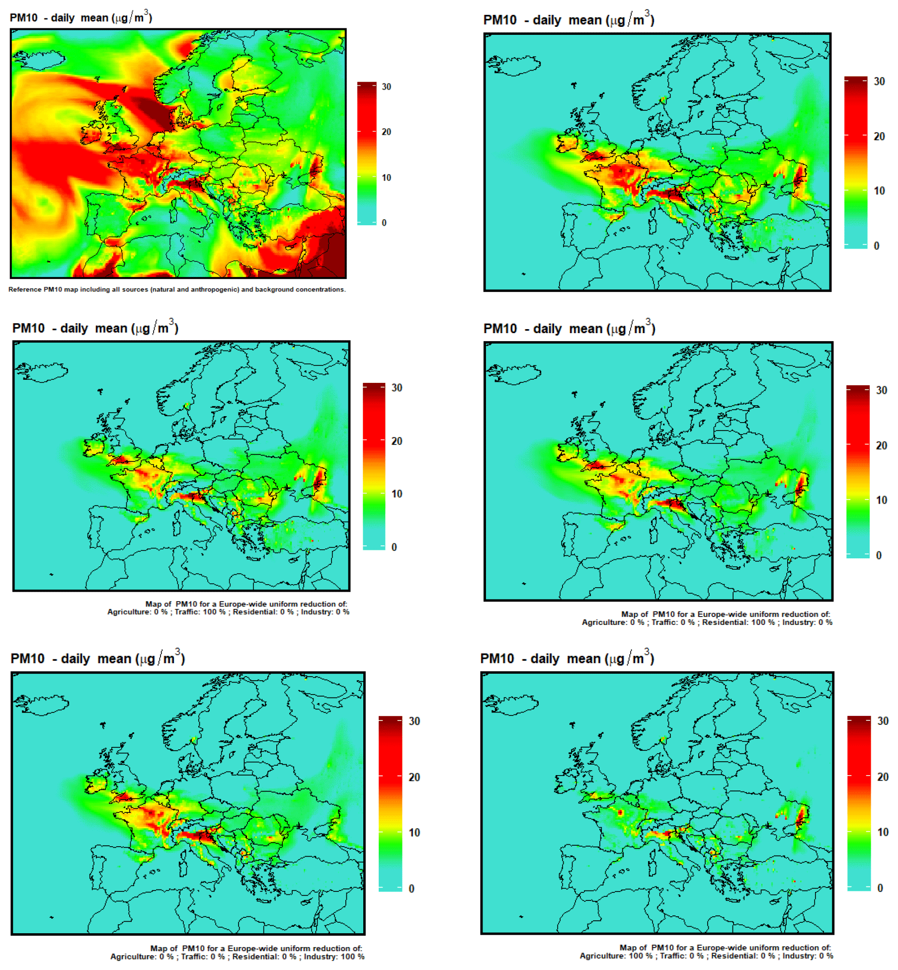
Figure 13First row: PM10 concentrations on 1 December 2016 including (left) or excluding (right) natural and background concentrations. Following rows: PM10 daily average concentrations emulated with ACT for 1 December 2016 for a 100 % reduction of traffic emissions (second row, left), residential emissions (second row, right), industry emissions (third row, left) and agriculture emissions (third row, right).
High PM10 concentrations are modelled over northern Italy but also a large part of northern France as well as the southwestern UK. There are also some scattered areas of pollution in eastern Ukraine. The removal of emission from each of the four main activity sectors is emulated with ACT in Fig. 13, using as reference the simulation excluding natural sources. All sectors have an influence on PM10 concentrations, but the largest contribution is attributed to agriculture, which is really the only source that has an impact on background PM10, although some hotspots remain. According to the scenario where a 100 % reduction of industrial emission in emulated, it seems that the PM10 peak in eastern Ukraine is due to industrial activities. The hotspots in Paris and Milan remain to some extent in all of the four scenarios, demonstrating that air pollution in those areas can only be mitigated by acting on all activity sectors.
The large role of agriculture is due to the high sensitivity of atmospheric chemistry to ammonia (NH3) emissions which reacts with nitrogen oxides emitted from any combustion source (traffic or other) to form ammonium nitrate. Given the strong seasonality of fertilizer spreading, ammonia emissions in December are likely due mainly to livestock emissions. The ACT results illustrate clearly the importance of agriculture for PM air pollution by allowing to emulate a scenario by removing all NH3 emissions. One should however keep in mind the challenge in mitigating NH3, where the emission reduction between 2005 and 2020 is only 1 % to 24 % in the Gothenburg protocol depending on the country (Bessagnet et al., 2014).
5.2.3 June 2017
For ozone, we selected the intense episode of June 2017 (Fig. 14) (Tarrason et al., 2017). An ozone anomaly above 60 to 70 µg m−3 was due to European emissions of the four main activity sectors, but Fig. 15 also highlights the importance of tropospheric burden for ozone air pollution where a large fraction cannot be mitigated by reducing European emissions alone.
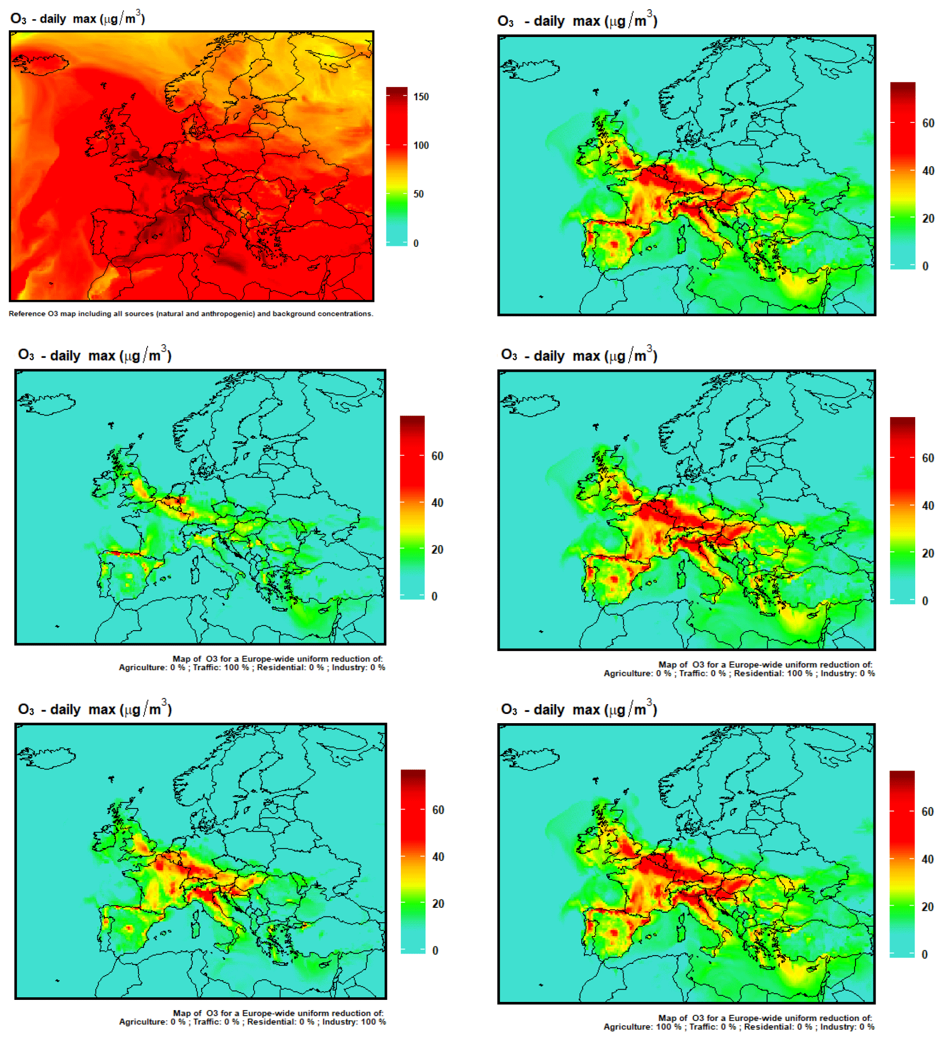
Figure 14First row: O concentrations on 21 June 2017 including (left) or excluding (right) natural and background concentrations. Following rows: O concentrations emulated with ACT for 21 June 2017 for a 100 % reduction of traffic emissions (second row, left), residential emissions (second row, right), industry emissions (third row, left) and agriculture emissions (third row, right).
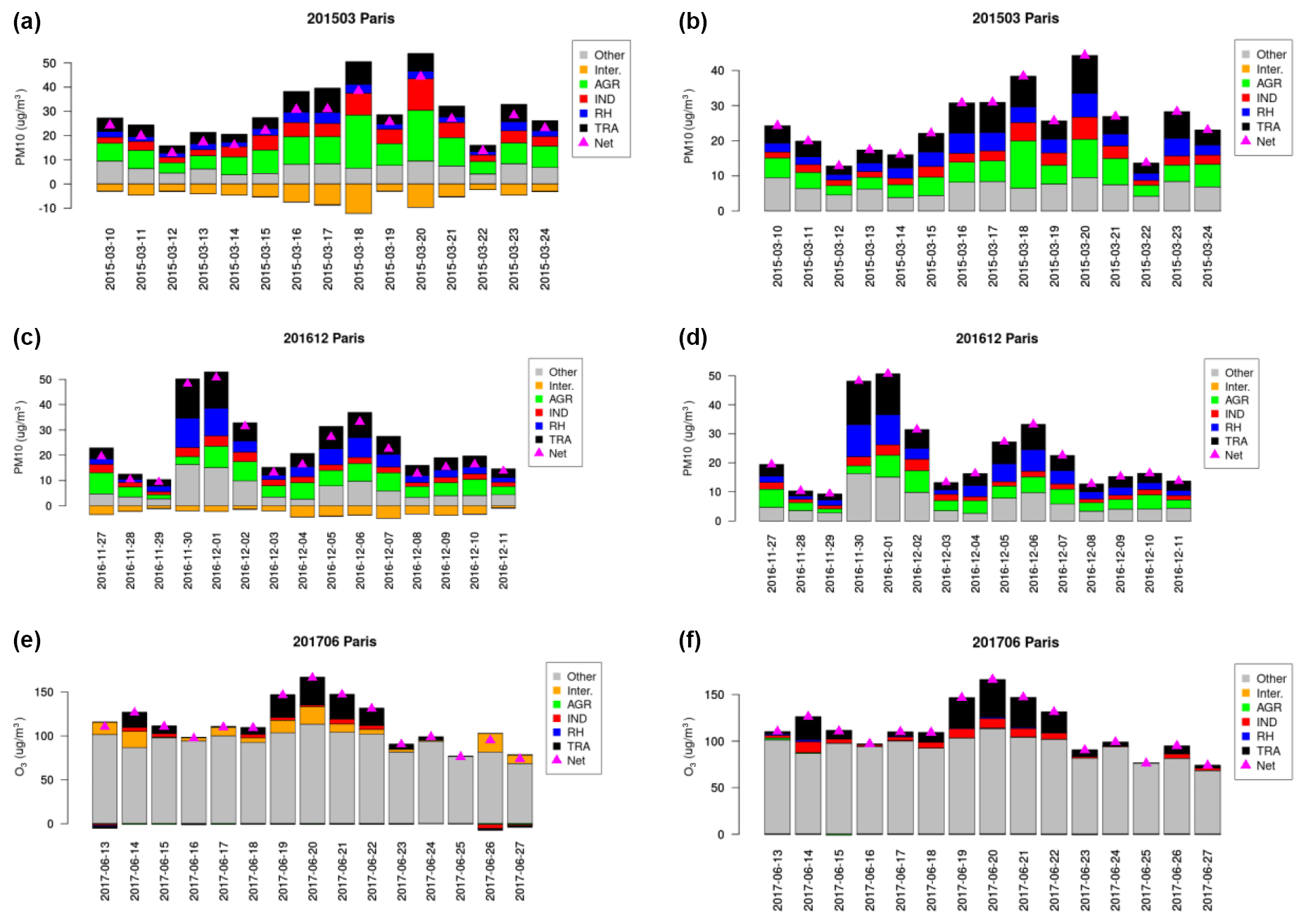
Figure 15Source allocation using the ACT surrogate model for PM10 in March 2015 (a, b) and December 2016 (c, d) and for O in June 2017 as in absolute levels (µg m−3) with explicit (a, c, e) or redistributed (b, d, f) interaction terms.
The analysis of emission reduction responses (Fig. 14) is much more predictable than the impact on PM. Reducing emissions from residential and agriculture sectors has almost no impact on ozone concentrations. Ozone is driven by emissions from traffic (nitrogen oxides) and from industry (nitrogen oxides and volatile organic compounds). For the case studied, removing traffic emissions decreases ozone concentrations by 20 to 60 µg m−3 in most of the places, and the impact is not as strong with a 100 % reduction in industry emissions.
The surrogate ACT model can also be used in source allocation mode. By reducing successively each activity sector by 100 %, it is possible to compute its contribution to the burden of air pollution for a given day and location. Here, the contribution would be the gain in concentration reduction induced by removing emissions from a given activity sector. It may differ substantially from a source apportionment approach where the objective is to assess the contribution – in mass – of a sector to the overall PM burden. A good illustration of such differences is the underestimation of the influence of a sector such as agriculture that only contributes with relatively light compounds in terms of molecular weight (NH3) but is very sensitive in the formation of secondary PM. The methodological difference and purposes are explained, for instance, in Clappier et al. (2017), which also emphasize the role of interaction terms further illustrated below.
Unlike source apportionment, the allocation we introduce here indeed shows the reduction of concentration that can be achieved by removing totally the emissions of an activity sectors. Such results are generally obtained by zeroing out anthropogenic emissions in a full CTM simulation. It can also be extrapolated from sensitivity simulation based only on 15 % to 30 % emission reductions. But then the uncertainties become substantial in the case of non-linear response. The structure of ACT, by being calibrated and tested for emission reductions ranging from 0 % to 100 %, offers a more reliable response in that context.
For the two PM10 episodes and the O3 episode introduced in Sect. 2.1 and for the city of Paris, we isolate in Fig. 15 the impact of each of the four activity sectors as well as natural and background concentrations. A specific focus is also given on how interaction terms are handled in this decomposition. In the left column, the gap between individual sectors and the overall reduction is explicitly provided as an interaction term. Here, the contribution of each activity sector is assessed by setting its emissions to zero (referred to as top-down brute force method in Clappier et al., 2017). Interactions are computed by difference between the sum of individual contribution and a scenario emulated with all four activity sector removed simultaneously (which is constrained by the scenario “AGR100IND100RH100TRA100”, Sect. 3.4). And the remaining fraction corresponds to natural sources or any other pollutant precursor not included in ACT (natural and background concentration).
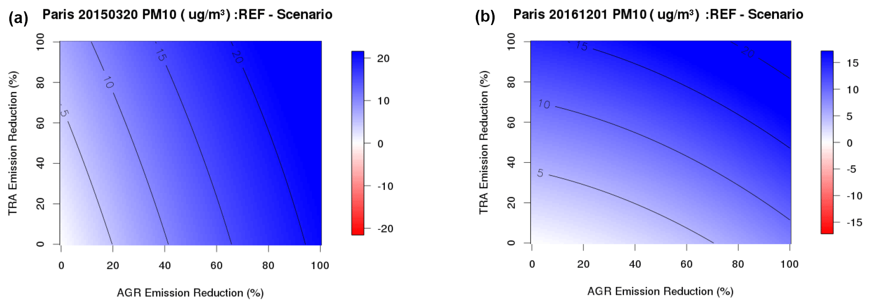
Figure 16PM10 concentration reduction (positive for a decrease in blue) corresponding to a given reduction in traffic and agriculture emissions over the Paris area – daily average for 20 March 2015 (a) and 1 December 2016 (b).
From this decomposition, the large influence of agriculture appears clearly for the March 2015 PM10 episode in Paris (Fig. 15). Traffic and industry are also important contributors, but residential heating has a smaller contribution. For the December 2016 PM10 episode, the agriculture contribution is only second behind traffic. Residential heating is more important than for the March 2015 episode, but it could also be underestimated by the model, which used an emission inventory that does not capture very well residential heating, in particular in relation with wood burning. This underestimation of residential emission has been widely documented as it has a very strong impact on model performance to capture wintertime peaks (Denier van der Gon et al., 2015). The expected future improvements in the consistency of reported condensable PM in emission inventories should notably improve model performance. Until then, this feature provides us with an opportunity to highlight that the diagnostics derived with the surrogate model remains highly sensitive to underlying hypotheses in emission inventories and chemistry-transport modelling.
For ozone, the picture is very different; a large fraction of ozone is actually attributed to the tropospheric burden. But during the ozone air pollution event (14 and 19–22 June), a larger contribution of traffic is found, whereas the impact of industry is very small (a different conclusion will hold for other cities as presented in Sect. 6). This presentation for ozone highlights very well the challenge of mitigating background levels on the basis of European emission mitigation. Conversely, it also shows precisely the need to act on European emission during the main ozone peak.
When interactions are negative, the sum of individual contribution of each activity sector exceed the total (“net”) in the reference simulation. It is clearly the case for the strong PM10 episode of March 2015, but conversely the interactions can also be positive as illustrated for the O3 episode of June 2017. The importance of interactions was expected considering the complexity of atmospheric chemistry. But it constitutes an artefact that must be dealt with when performing a source allocation by treating each sector independently.
There is no fully satisfactory approach to handle interaction terms in such a decomposition. The simplest alternative is to distribute one-fourth of those interactions into each of the four contributions which leads to rescaling the reference simulation (Table 4). The contribution of individual sector can change substantially, which is also a reminder for the overall uncertainty of the approach. For instance, the share of agriculture is reduced from 32 % to 23 % in the case of the March 2015 PM episode. But at least the ranking of each sector is not changed and their qualitative evolution, displayed in the right column of Fig. 15, is similar.
Table 4Relative contributions (%) of the four main activity sectors as well as natural and background concentrations (“other”) averaged over the three selected air pollution episodes, either with explicit interaction terms or with interactions redistributed within individual contributions.

The surrogate ACT model trained on CHIMERE sensitivity simulations also allows exploring the chemical sensitivity (or regimes) within the parameter space of sectoral emission reductions. ACT is a quadrivariate second-order polynomial with interactions using as predictors the four sectors considered. By plotting the surface response to two of these four sectors in a 2-D parameter space, it is possible to assess chemical regimes for a given day, location and pollutant. In doing so, we perform an analogy with the classical ozone production isopleths of Sillman (1999) by substituting the NOx and VOC emissions in the x and y axes by different activity sectors.
Figure 16 compares two particulate pollution days, over Paris areas, in March 2015 and December 2016, respectively. In March 2015, reducing agriculture emissions has a strong positive impact on the reduction of PM10 concentrations that decrease sharply, while the impact of traffic emissions reduction is much less effective with the isopleth close to vertical lines. The inverse conclusions can be drawn for the December 2016 episode, where a linear decrease of PM10 is induced by traffic emission reductions, whereas the isopleths are closer to horizontal lines, depicting a low sensitivity to agricultural emission changes.
Ozone chemical regimes can also be investigated for a high-ozone episode (21 June 2017), for various locations and for both ozone daily maxima and daily means (Fig. 17).
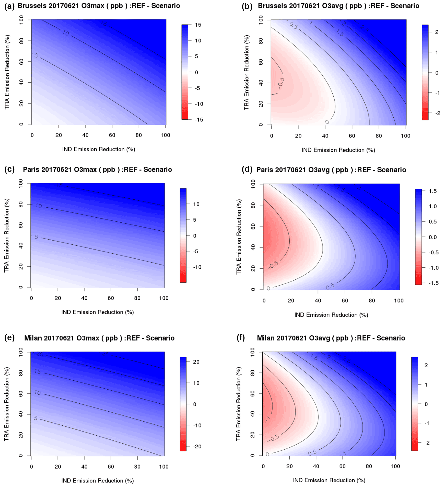
Figure 17Same as Fig. 16 for ozone daily maximum (a, c, e) and ozone daily mean (b, d, f) and Brussels, Paris and Milan for a high-ozone day (21 June 2017).
Chemical regimes leading to the formation of high-ozone values (as the slope of isopleths for daily maximum ozone) are quite similar over Paris and Milan. But in Brussels a stronger sensitivity to industrial emissions is found. The isopleths for daily average ozone on the same day are very different. For all levels of industrial emissions, we find that a decrease of traffic emissions leads first to an increase of ozone before becoming efficient for the largest levels of emission reduction.
We presented the first surrogate air quality model designed to explore custom air pollution mitigation scenarios in the every-day air quality forecast. This tool applies for PM10, PM2.5, O3 (both as daily mean and daily maximum) and NO2, and covers the following activity sectors: agriculture, industry, road transportation and residential heating. It can be implemented within an operational air quality forecasting system and operated interactively by any user through a web interface (https://policy.atmosphere.copernicus.eu/CAMS_ACT.php, last access: 1 February 2022).
Because of the complexity of atmospheric chemistry and physics, chemistry-transport models are required to account for the fate of air pollutants in the atmosphere. Simplified models have been developed over the past for assessment purposes, for instance, to identify optimal long-term mitigation strategies. However, such simplified models rely on assumptions which are not valid over short time periods, such as the linearity of the response of air concentrations to incremental emission changes.
We introduce a new surrogate modelling approach, whose main strength is to apply for short timescales, so that it can be embedded in an air quality forecast system. This challenge is achieved by calibrating every day a new surrogate model on the basis of the forecast of the corresponding day. Most of the complexity of atmospheric processes remains therefore represented within the full chemistry-transport model, and the only purpose of the surrogate is to offer flexibility.
First, we investigated the non-linearity of the response of atmospheric pollutant concentrations to incremental emission changes for various pollutants, areas and different episode typologies. We concluded that whereas the response was mainly linear for residential heating, non-linearities were important, especially for agriculture emissions and their impact on PM10 formation, and traffic and industrial emissions for ozone pollution.
The numerical experiment plan to identify the best model structure and the corresponding optimal set of training scenarios is presented by increasing level of complexity. We ultimately select a quadrivariate polynomial of first order for residential heating emissions and second order for agriculture, industry and traffic emissions with three interaction terms. The surrogate is trained on 10 sensitivity simulations, to which a reference and a closure simulation must be added. With such a structure, we can ensure that relative errors remain below 2 % at 95 % of the grid points and days for PM10, PM2.5, NO2, O and O.
The user interface is available online and a few case studies are presented. The emulation of custom scenarios is introduced for two PM10 and one ozone episode. It highlights the important role of agricultural emission in the formation of regional-scale PM episodes, although several hotspots can only be mitigated by acting on all sectors. For ozone, the tropospheric burden is important, but during a strong air pollution episode, action on European sources of traffic and industry can reduce peak levels.
The surrogate model can also be used for source allocation, although it requires additional assumptions on the way interaction terms are handled. We also present an innovative application for chemical regime analysis for both ozone and particulate air pollution, providing new insight on the identification of the most efficient activity sector to be targeted for air pollution episode mitigation.
At present, the main limitation of ACT is that it relies on emission reductions that are uniform over Europe. Adding geographical flexibility is one of the priorities for further development.
To our knowledge, this model is the first surrogate, or emulator, able to cover a short timescale for air pollution studies. This development was only made possible by assuming uniform and constant emission reductions for the four targeted activity sectors. The fact that emission reductions are assumed to be applied over the long term makes ACT not suited to assess the benefit of emergency measures to mitigate air pollution episodes. The purpose of the tool is rather to assess the main activity sectors driving the day-to-day air pollution variability.
Although the structure of the model is determined once by the outcome of the present study, the surrogate is calibrated every day to a new air quality forecast, therefore paving the way to further develop machine learning in the field of air quality forecasting.
The script used for the operational daily training of the ACT surrogate is available at https://github.com/acolette/ACT_v1.0 (last access: 15 February 2022) (https://doi.org/10.5281/zenodo.5973299, Colette, 2022). The underlying CHIMERE chemistry-transport model is available at https://www.lmd.polytechnique.fr/chimere/chimere.php (Mailler et al., 2017).
The modelling results used in the present study are archived by the authors and can be obtained from the corresponding author upon request.
The supplement related to this article is available online at: https://doi.org/10.5194/gmd-15-1441-2022-supplement.
AC conceptualized the model, designed the experiment and performed the simulations with support of FM. VL and BR designed the interface of the web toolbox. AC and LR prepared the manuscript with contributions from all co-authors.
The contact author has declared that neither they nor their co-authors have any competing interests.
Publisher’s note: Copernicus Publications remains neutral with regard to jurisdictional claims in published maps and institutional affiliations.
The high-performance simulations were performed on the Centre de Calcul Recherche et Technologie.
The present work was funded under the Copernicus Atmosphere Monitoring Service Policy Support contract (CAMS_71), also benefiting from the support of the French Ministère de la Transition Ecologique.
This paper was edited by Ignacio Pisso and reviewed by two anonymous referees.
Amann, M., Bertok, I., Cofala, J., Heyes, C., Klimont, Z., Rafaj, P., Schöpp, W., and Wagner, F.: National Emission Ceilings for 2020 Based on the 2008 Climate and Energy Package, IIASA, Laxenburg, 2008.
Amann, M., Bertok, I., Borken-Kleefeld, J., Cofala, J., Heyes, C., Höglund-Isaksson, L., Klimont, Z., Nguyen, B., Posch, M., Rafaj, P., Sandler, R., Schöpp, W., Wagner, F., and Winiwarter, W.: Cost-effective control of air quality and greenhouse gases in Europe: Modeling and policy applications, Environ. Modell. Softw., 26, 1489–1501, 2011.
Bessagnet, B., Beauchamp, M., Guerreiro, C., de Leeuw, F., Tsyro, S., Colette, A., Meleux, F., Rouïl, L., Ruyssenaars, P., Sauter, F., Velders, G. J. M., Foltescu, V. L., and van Aardenne, J.: Can further mitigation of ammonia emissions reduce exceedances of particulate matter air quality standards?, Environ. Sci. Policy, 44, 149–163, 2014.
Clappier, A., Belis, C. A., Pernigotti, D., and Thunis, P.: Source apportionment and sensitivity analysis: two methodologies with two different purposes, Geosci. Model Dev., 10, 4245–4256, https://doi.org/10.5194/gmd-10-4245-2017, 2017.
Cohan, D. S. and Napelenok, S. L.: Air Quality Response Modeling for Decision Support, Atmosphere, 2, 407–425, 2011.
Colette, A.: acolette/ACT_v1.0: Air Control Toolbox (ACT_v1.0) (V1.0), Zenodo [code], https://doi.org/10.5281/zenodo.5973299, 2022.
Colette, A., Granier, C., Hodnebrog, Ø., Jakobs, H., Maurizi, A., Nyiri, A., Rao, S., Amann, M., Bessagnet, B., D'Angiola, A., Gauss, M., Heyes, C., Klimont, Z., Meleux, F., Memmesheimer, M., Mieville, A., Rouïl, L., Russo, F., Schucht, S., Simpson, D., Stordal, F., Tampieri, F., and Vrac, M.: Future air quality in Europe: a multi-model assessment of projected exposure to ozone, Atmos. Chem. Phys., 12, 10613–10630, https://doi.org/10.5194/acp-12-10613-2012, 2012.
Colette, A., Andersson, C., Baklanov, A., Bessagnet, B., Brandt, J., Christensen, J. H., Doherty, R., Engardt, M., Geels, C., Giannakopoulos, C., Hedegaard, G. H., Katragkou, E., Langner, J., Lei, H., Manders, A., Melas, D., Meleux, F., Rouïl, L., Sofiev, M., Soares, J., Stevenson, D. S., Tombrou-Tzella, M., Varotsos, K. V., and Young, P.: Is the ozone climate penalty robust in Europe?, Environ. Res. Lett., 10, 084015, https://doi.org/10.1088/1748-9326/10/8/084015, 2015.
Denier van der Gon, H. A. C., Bergström, R., Fountoukis, C., Johansson, C., Pandis, S. N., Simpson, D., and Visschedijk, A. J. H.: Particulate emissions from residential wood combustion in Europe – revised estimates and an evaluation, Atmos. Chem. Phys., 15, 6503–6519, https://doi.org/10.5194/acp-15-6503-2015, 2015.
Engelen, R. J. and Peuch, V.: The Copernicus Atmosphere Monitoring Service: facilitating the prediction of air quality from global to local scales, AGU Fall Meeting Abstracts, San Francisco, December 2017, American Geophysical Union, Fall Meeting, abstract #A31N-02, 2017.
Forêt, G., Haeffelin, M., Kreitz, M., Boucher, O., Beekmann, M., Formenti, P., Bodichon, R., Dupont, J. C., Drouin, M. A., Bravo-Aranda, J. A., Favez, O., Ghersi, V., Gratien, A., Michoud, V., Gros, V., and Té, Y.: Analyse préliminaire de l'épisode de pollution francien de décembre 2016, La Météorologie, 96, 11–15, https://doi.org/10.4267/2042/61967, 2017.
Kuenen, J. J. P., Visschedijk, A. J. H., Jozwicka, M., and Denier van der Gon, H. A. C.: TNO-MACC_II emission inventory; a multi-year (2003–2009) consistent high-resolution European emission inventory for air quality modelling, Atmos. Chem. Phys., 14, 10963–10976, https://doi.org/10.5194/acp-14-10963-2014, 2014.
Mailler, S., Menut, L., Khvorostyanov, D., Valari, M., Couvidat, F., Siour, G., Turquety, S., Briant, R., Tuccella, P., Bessagnet, B., Colette, A., Létinois, L., Markakis, K., and Meleux, F.: CHIMERE-2017: from urban to hemispheric chemistry-transport modeling, Geosci. Model Dev., 10, 2397–2423, https://doi.org/10.5194/gmd-10-2397-2017, 2017 (data available at: https://www.lmd.polytechnique.fr/chimere/chimere.php, last access: 15 February 2022).
Marécal, V., Peuch, V.-H., Andersson, C., Andersson, S., Arteta, J., Beekmann, M., Benedictow, A., Bergström, R., Bessagnet, B., Cansado, A., Chéroux, F., Colette, A., Coman, A., Curier, R. L., Denier van der Gon, H. A. C., Drouin, A., Elbern, H., Emili, E., Engelen, R. J., Eskes, H. J., Foret, G., Friese, E., Gauss, M., Giannaros, C., Guth, J., Joly, M., Jaumouillé, E., Josse, B., Kadygrov, N., Kaiser, J. W., Krajsek, K., Kuenen, J., Kumar, U., Liora, N., Lopez, E., Malherbe, L., Martinez, I., Melas, D., Meleux, F., Menut, L., Moinat, P., Morales, T., Parmentier, J., Piacentini, A., Plu, M., Poupkou, A., Queguiner, S., Robertson, L., Rouïl, L., Schaap, M., Segers, A., Sofiev, M., Tarasson, L., Thomas, M., Timmermans, R., Valdebenito, Á., van Velthoven, P., van Versendaal, R., Vira, J., and Ung, A.: A regional air quality forecasting system over Europe: the MACC-II daily ensemble production, Geosci. Model Dev., 8, 2777–2813, https://doi.org/10.5194/gmd-8-2777-2015, 2015.
Menut, L., Bessagnet, B., Khvorostyanov, D., Beekmann, M., Blond, N., Colette, A., Coll, I., Curci, G., Foret, G., Hodzic, A., Mailler, S., Meleux, F., Monge, J.-L., Pison, I., Siour, G., Turquety, S., Valari, M., Vautard, R., and Vivanco, M. G.: CHIMERE 2013: a model for regional atmospheric composition modelling, Geosci. Model Dev., 6, 981–1028, https://doi.org/10.5194/gmd-6-981-2013, 2013.
Petit, J. E., Amodeo, T., Meleux, F., Bessagnet, B., Menut, L., Grenier, D., Pellan, Y., Ockler, A., Rocq, B., Gros, V., Sciare, J., and Favez, O.: Characterising an intense PM pollution episode in March 2015 in France from multi-site approach and near real time data: Climatology, variabilities, geographical origins and model evaluation, Atmos. Environ., 155, 68–84, https://doi.org/10.1016/j.atmosenv.2017.02.012, 2017.
Pisoni, E., Clappier, A., Degraeuwe, B., and Thunis, P.: Adding spatial flexibility to source-receptor relationships for air quality modeling, Environ. Modell. Softw., 90, 68–77, https://doi.org/10.1016/j.envsoft.2017.01.001, 2017.
Rouïl, L., Honore, C., Vautard, R., Beekmann, M., Bessagnet, B., Malherbe, L., Meleux, F., Dufour, A., Elichegaray, C., Flaud, J. M., Menut, L., Martin, D., Peuch, A., Peuch, V. H., and Poisson, N.: PREV'AIR An Operational Forecasting and Mapping System for Air Quality in Europe, B. Am. Meteorol. Soc., 90, 73–83, 10.1175/2008bams2390.1, 2009.
Sillman, S.: The relation between ozone, NOx and hydrocarbons in urban and polluted rural environments, Atmos. Environ., 33, 1821–1845, 1999.
Tarrason, L., Hamer, P., Rouïl, L., and Meleux, F.: Interim Annual Assessment Report for 2017, European air quality in 2017, available at: https://policy.atmosphere.copernicus.eu/reports/CAMS-71_SC12019_D1.2.1-2017_202004_V1.pdf (last access: 15 February 2022), 2017.
Thunis, P., Clappier, A., Pisoni, E., and Degraeuwe, B.: Quantification of non-linearities as a function of time averaging in regional air quality modeling applications, Atmos. Environ., 103, 263–275, 2015.
Zhang, Y., Bocquet, M., Mallet, V., Seigneur, C., and Baklanov, A.: Real-time air quality forecasting, part I: History, techniques, and current status, Atmos. Environ., 60, 632–655, 2012.
- Abstract
- Introduction
- Methods
- Design of the optimal surrogate model
- Final structure and performance
- Scenario analysis in air quality forecasts
- Source allocation mode
- Chemical regimes
- Conclusion
- Code availability
- Data availability
- Author contributions
- Competing interests
- Disclaimer
- Acknowledgements
- Financial support
- Review statement
- References
- Supplement