Definitions and methods to estimate regional land carbon fluxes for the second phase of the REgional Carbon Cycle Assessment and Processes Project (RECCAP-2)

Regional land carbon budgets provide insights into the spatial distribution of the land uptake of atmospheric carbon dioxide and can be used to evaluate carbon cycle models and to define baselines for land-based additional mitigation efforts. The scientific community has been involved in providing observation-based estimates of regional carbon budgets either by downscaling atmospheric CO₂ observations into surface fluxes with atmospheric inversions, by using inventories of carbon stock changes in terrestrial ecosystems, by upscaling local field observations such as flux towers with gridded climate and remote sensing fields, or by integrating data-driven or process-oriented terrestrial carbon cycle models. The first coordinated attempt to collect regional carbon budgets for nine regions covering the entire globe in the RECCAP-1 project has delivered estimates for the decade 2000–2009, but these budgets were not comparable between regions due to different definitions and component fluxes being reported or omitted. The recent recognition of lateral fluxes of carbon by human activities and rivers that connect CO₂ uptake in one area with its release in another also requires better definitions and protocols to reach harmonized regional budgets that can be summed up to a globe scale and compared with the atmospheric CO₂ growth rate and inversion results. In this study, using the international initiative RECCAP-2 coordinated by the Global Carbon Project, which aims to be an update to regional carbon budgets over the last 2 decades based on observations for 10 regions covering the globe with a better harmonization than the precursor project, we provide recommendations for using atmospheric inversion results to match bottom-up carbon accounting and models, and we define the different component fluxes of the net land atmosphere carbon exchange that should be reported by each research group in charge of each region. Special attention is given to lateral fluxes, inland water fluxes, and land use fluxes.

1 Introduction

The objective of this paper is to define the land–atmosphere CO₂ or total carbon (C) fluxes to be used in the REgional Carbon Cycle Assessment and Processes-2 (RECCAP2) project. Accurate and consistent observation-based estimates of terrestrial carbon budgets at regional scales are needed to understand the global land carbon sink, to evaluate land carbon models used for carbon budget assessments and future climate projections, and to define baselines for land-based mitigation efforts. In the previous synthesis, RECCAP1, regional data from inventories were compared with global models output from atmospheric inversions and process-based land models, with the results for 9 land regions in the period 2000–2009 being synthesized in a special issue (https://bg.copernicus.org/articles/special_issue107.html, last access: November 2021​​​​​​​). The definition of fluxes was not harmonized, and inland waters and trade-induced CO₂ fluxes were not considered for most regions. The RECCAP1 synthesis spurred efforts to provide new global analysis of inland water CO₂ fluxes (Raymond et al., 2013). Recently, Ciais et al. (2020) collected bottom-up inventory estimates from RECCAP1 papers and completed them with other components to derive the first global bottom-up estimate of the net land atmosphere C exchange, which compared well with the independent top-down estimate obtained from the CO₂ growth rate minus fossil fuel emissions and ocean uptake.

The aims of RECCAP2 are to collect and synthesize regional CO₂, CH₄, and N₂O budgets for 10 continental-scale regions (including one “cross-cutting” region consisting of all permafrost-covered boreal areas) that together cover the globe (Fig. 1). There is thus a requirement for sufficient harmonization and consistency to be able to scale regional budgets to the globe and to compare different regions with each other for all component fluxes and each greenhouse gas. In RECCAP-2, the results of top-down atmospheric inversions will also be compared with bottom-up accounting approaches. Since research groups working on the synthesis of greenhouse gas budgets in different regions or using different approaches use different datasets and definitions, it is important to provide a set of shared and agreed definitions that are as precise as possible for each flux to be reported. We focus here on land C and CO₂ budgets, defined from two approaches: “top-down” estimates from atmospheric inversions and “bottom-up” carbon accounting approaches based on C stock inventories and process- and data-oriented models.

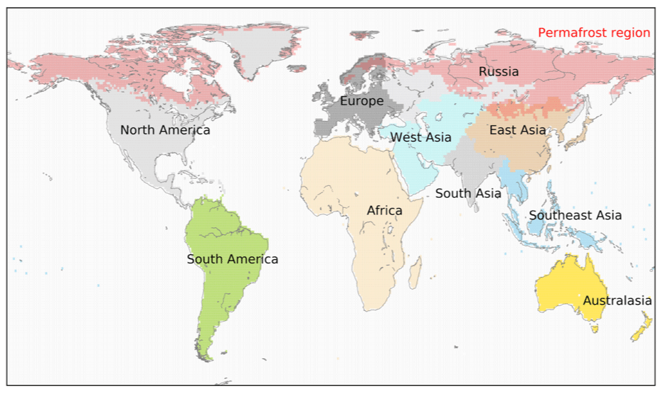
Figure 1 Map of the RECCAP2 regions. The “region” in red corresponds to permafrost-covered areas. Map plot courtesy of Naveen Chandra (NIES/JAMSTEC).

Additionally, we propose guidelines to separate and quantify the different gross fluxes that compose the net budget. Such attribution can be done by process (e.g., photosynthesis, soil respiration, fires, etc) or by cause (natural vs. anthropogenic). Each approach responds to specific objectives, e.g., attribution by cause being crucial for national greenhouse gas (GHG) accounting, but also reflects practical considerations on how to measure or quantify certain fluxes. For example, biomass combustion fluxes can be a result of climate variations or of land use change and management, but separating these causes is challenging since they co-vary and current scientific methods cannot separate the two. Attribution by cause is usually based in national inventories on the definition of “managed” and “unmanaged land” proxies, which can lead to inconsistencies between different estimates (Grassi et al., 2018). In RECCAP-2, we propose a process-based approach whenever possible and separation by cause only when required by the existing methods for flux estimation.

Estimates of land–atmosphere CO₂ fluxes by atmospheric inversions inherently differs from bottom-up C budgets for two reasons. The first reason is the existence of lateral fluxes at the land surface and from the land to the ocean, which displace carbon initially fixed as CO₂ from the atmosphere in one region and release it outside that region. Consequently, the CO₂ flux diagnosed by an inversion is not equal to the change of stock in a region. The second reason is that carbon enters from the atmosphere in the land reservoirs almost uniquely as CO₂ fixed by photosynthesis, while it is released both as CO₂ and as reduced carbon compounds encompassing CO, CH₄, and biogenic volatile organic compounds (BVOCs). This process again makes CO₂ fluxes different from total carbon fluxes across the land–atmosphere surface.

To address these issues, Sect. 1 of this paper covers atmospheric CO₂ inversions and the treatment of reduced C compound emissions, with the goal of making inversion results comparable with total C flux estimates from bottom-up approaches. Section 2 deals with bottom-up estimates and provides definitions of the main component land–atmosphere C fluxes that should be estimated individually to provide a full assessment of the C balance of each region and to enable consistent comparisons between regions and upscaling of regional budgets to the globe. Section 3 provides a description of different approaches used to derive regional component C fluxes in different bottom-up approaches, outlining which fluxes are included or ignored by each different approach. Section 4 gives recommendations regarding the estimation of carbon emissions resulting from land use change, with systematic errors and omission errors associated to different approaches. We conclude by providing recommendations for a multiple-tier approach to develop regional C budgets in RECCAP2.

2 Top-down land–atmosphere C fluxes from atmospheric inversions

2.1 Land CO₂ fluxes covered by inversions

The​​​​​​​ approaches known as top-down atmospheric inversions estimate the net CO₂ flux exchanged between the surface and the atmosphere by using atmospheric transport models and CO₂ mole fraction measurements at various locations. The mole fraction data come from surface stations, which have been available in increasing numbers since 1957. More recently, total column mole fraction of CO₂ have been observed with global coverage by satellites, e.g., GOSAT since 2009 and OCO-2 since 2014 (Liu et al., 2021). Because the sampling of the atmosphere is sparse even with the recent global satellite observations, there is an infinite number of flux combinations that can fit atmospheric CO₂ observations within their errors. Most inversions therefore use a Bayesian statistical approach where an optimal CO₂ flux is found as a maximum likelihood estimate in the statistical distribution of possible fluxes, given the prior value and its uncertainty distribution, and observations, which also have an uncertainty distribution. The effect of fossil fuel and cement production CO₂ emissions (hereafter collectively called “fossil fuel” for simplicity) on mixing ratio gradients is accounted for by prescribing transport models with an assumed fixed map of fossil CO₂ emissions. The signal from these emissions in the space of concentrations is removed at the pre- or post-processing stage from inversions to solve for residual non-fossil CO₂ fluxes. Over land, output fluxes from inversions are thus the sum of all non-fossil CO₂ fluxes. This includes gross primary production CO₂ uptake, plant and soil respiration, litter photo-oxidation, biomass burning emissions both from wildfires and for the purposes of energy provision, inland water fluxes, the oxidative release of CO₂ from biomass consumed by animals and humans and decaying in waste pools, CO₂ emitted by insect grazing, geological CO₂ emissions from volcanoes and seepage from belowground sources, CO₂ uptake from weathering reactions, and geological CO₂ release from microbial oxidation of petrogenic carbon (Hemingway et al., 2018). Inversions have very limited capability to separate those different fluxes unless they use additional information, which is not the case for inversions used in global budgets. An example of additional information is the use of CO as a tracer to separate emissions from vegetation fires from those from fossil fuels and respiration.

Atmospheric inversion models provide CO₂ fluxes over all land (and ocean) grid cells, whereas national inventories estimate carbon stock changes over managed land only. Managed land is used by countries as a proxy to separate “direct human-induced effects” from “indirect effects” leading to carbon stock changes. If the purpose is to compare inversions with national inventories (e.g., Deng et al. 2021), we recommend using spatially explicit managed land masks and applying them to gridded inversions fluxes. Some (but not all) countries provided such datasets (Ogle et al., 2018). One approximation for defining managed lands in the absence of national gridded areas could be to use masks of intact forests (Potapov et al., 2017) with some adjustment to match reported national totals.

2.2 Prescribing fossil CO₂ emission fields that include bunker fuels

Within RECCAP1 (Canadell et al., 2015) the same fossil fuel emission estimate was subtracted from the total posterior fluxes of participating inversions, even when those inversions had used different fossil fuel inventories (Peylin et al., 2013). This inconsistency between the inversion process and the inversion post-processing induced artifacts (see discussion in Thompson et al., 2016) but is of lesser importance for the intercomparison than the use of different fossil fuel inventories within the inversion ensemble. We thus recommend here that a standard gridded a priori fossil fuel CO₂ emission estimate is used by all regions in RECCAP2, such as the one recently prepared by Jones et al. (2021). Another important issue is that about 10 % of CO₂ emissions come from mobile sources, from ships on the ocean surface, and aircraft in the volume of the atmosphere. We recommend that these “bunker fuel” emissions are prescribed to RECCAP2 inversions by using three-dimensional maps of fossil fuel CO₂ emissions. Each grid box should thus include the emissions within its borders, along ship routes on the surface, and flight paths at the appropriate altitude in the atmosphere. This option is increasingly viable due to the emerging availability of sectoral emissions grids for recent years (Choulga et al., 2021; Jones et al., 2021).

2.3 Reduced C compound emissions

Reduced C compounds are emitted by the land surface as biogenic and anthropogenic CH₄, BVOCs, and CO. Globally, emissions of reduced C compounds from land ecosystems and fossil fuel use are a large and overlooked component of the C budget, with CO carbon emissions from incomplete fuel combustion equaling ≈0.3 PgC yr⁻¹ (Zheng et al., 2019), CH₄ carbon emissions equaling 0.43 PgC yr⁻¹ (Saunois et al., 2020), and non-methane biogenic compounds emissions that total up to 0.75 PgC yr⁻¹ (Sindelarova et al., 2014). Given that inversions only assimilate atmospheric observations of CO₂, they omit regional emissions of reduced C compounds. However, reduced C compounds all oxidize to CO₂ in the atmosphere, with lifetimes of hours to days for BVOCs, months for CO, and nearly 10 years for CH₄. The global CO₂ growth rate thus includes the signal of the global reduced C emissions being oxidized into CO₂ in the volume of the atmosphere, though not necessarily in the year of their emission. By fitting the global CO₂ growth rate, inversions thus include global emission of reduced C compounds, which is diagnosed as a diffuse natural CO₂ emission over the whole surface of the globe in that year. This implies that inversions place an incorrect ocean CO₂ emission in the place of reduced C compounds emitted only over land (Enting and Mansbridge, 1991). Further, current inversions assume that all the fossil C is emitted as CO₂, ignoring incomplete fuel combustion emitted as CO. The signal from fossil fuel CO emissions on the CO₂ concentration field is therefore incorrectly treated as a surface emission of fossil CO₂. Such an overestimation of fossil CO₂ emissions at the surface, mainly over Northern Hemisphere large fossil-fuel-emitting regions, leads to an overestimation of the surface CO₂ sink in order to match the interhemispheric CO₂ gradient.

A mathematical formulation of the effect of CO emissions and oxidation on the latitudinal gradient of atmospheric CO₂ and its impact on natural CO₂ fluxes in a 2D inversion ignoring incomplete fuel combustion emitted as CO that amounts to ≈0.3 PgC (latitude-vertical) was given by Enting and Mansbridge (1991). They showed that an inversion that includes an atmospheric CO loop of the carbon cycle placed a larger surface CO₂ sink in the northern tropics and a smaller surface CO₂ sink north of 50^∘ N compared to an inversion without this process. Using a 3D inversion, Suntharalingam et al. (2005) confirmed the impact of CO oxidation in the atmosphere, albeit with modest effects on diagnosed land CO₂ fluxes. We describe an approach to correct for the effect of BVOCs, CO, and CH₄ in inversions for RECCAP2 below. This approach allows the translation of current inversions CO₂ fluxes into total C fluxes that can then be consistently compared with total C fluxes given by bottom-up approaches.

2.4 Correcting net CO₂ ecosystem exchange from inversions for reduced compounds

Separate corrections to inversions should be made for BVOCs, CO, and CH₄ because they have very different lifetimes and thus affect the CO₂ mole fraction gradients measured by surface networks or satellites in different ways. Most BVOCs have a short lifetime and are oxidized to CO₂ in the boundary layer. This means that inversions using CO₂ concentration observations interpret BVOC emissions as local surface CO₂ emissions. Globally, carbon emissions from VOCs amount to 0.8 PgC yr⁻¹; are mostly biogenic (Guenther et al., 2012); and are dominated by isoprene, methanol, and terpenes (Folberth et al., 2005). If the purpose is to compare inversions to net ecosystem exchange (NEE) of total C derived from bottom-up methods (see Sect. 2​​​​​​​), we recommend including BVOC carbon emissions in bottom-up regional estimates of NEE, rather than making BVOC correction of inversion CO₂ fluxes.

Regarding the effect of the fossil CO loop of the atmospheric CO₂ cycle mentioned above, we propose treating fossil CO as a “bunker fuel”. First, we have to reduce the prescribed prior gridded fossil CO₂ emissions by the gridded amount emitted as CO using the space–time distribution of this CO source from inventories or from fossil CO emission inversion results. Following this, we have to prescribe a compensatory prior 3D atmospheric CO₂ source originating from fossil CO oxidized by OH in the atmosphere. Knowledge of this prior 3D source of CO₂ from the fossil origin is now available from the atmospheric chemistry models used by global fossil CO emissions inversions since 2000 (Zheng et al., 2019). Other chemistry transport models simulating the atmospheric oxidation chain of reduced C compounds unconstrained by observations may not be accurate enough for that purpose (Stein et al., 2014). We thus recommend developing new fossil CO₂ emission prior fields for RECCAP2 that include the fossil CO loop. The impact of such new priors will be to reduce inversion estimates of natural CO₂ sinks in the Northern Hemisphere over regions where fossil fuels are burned and to enhance sinks in the tropics and subtropics where CO is oxidized into CO₂.

Regarding the effect of CO emissions from wildfires, which ranges globally from 0.15 to 0.3 PgC yr⁻¹ (Zheng et al., 2019; van der Werf et al., 2017), the action to be taken for inversions depends on the configuration of each system, since inversions do not all use a prior fire emission map, in which case CO from fires could be treated like CO from fossil fuels as explained above. Looking into the three global inversions used in previous global carbon budget assessments, the Jena CarboScope inversion (Rödenbeck et al., 2003) does not have biomass burning a priori CO₂ emissions. The CarbonTracker Europe (CTE) inversion (Peters et al., 2010; van der Laan-Luijkx et al., 2017​​​​​​​) prescribes temporal and spatial prior fire emissions, which means that any CO₂ uptake by vegetation regrowth after fire will be spread as a diffuse CO₂ sink within and outside burned regions. The CAMS inversion (Chevallier, 2019) prescribes temporal and spatial prior fire emissions and an annual CO₂ uptake equal to annual emissions over each grid cell affected by fires. This setting of CAMS forces an annual regrowth of forests after burning but allows the inversion to temporally allocate this regrowth uptake. CTE and CAMS consider all prior fire emissions as CO₂ emissions, ignoring incomplete combustion emissions of CO. Thus, just as in fossil CO₂ emissions, CTE and CAMS inversions will overestimate the prior values of CO₂ mixing ratios over burned areas during the fire season. Given the lifetime of CO and the fact that most biomass burning takes place in the tropics, prescribing all prior fire emissions as CO₂ in CTE and CAMS will cause only a small positive bias in prior CO₂ mixing ratio at tropical stations. The situation may be different for satellite inversions assimilating column CO₂ data. These inversions sample CO₂ plumes resulting from biomass burning but not co-emitted CO. In this case, it is expected that inversions based on satellite observations will capture biomass burning CO₂ emissions but underestimate fire C emissions by the amount of CO emitted by fires. Carbon emitted as CO by fires will contribute after its oxidation to the global CO₂ growth rate. This signal will thus be wrongly interpreted by inversions as a diffuse CO₂ source spread uniformly over land and ocean. For RECCAP2, we recommend pursuing research to include CO₂ fluxes from the fire CO loop as a prior field to be tested by the inversions that already have fire prior emissions in their settings.

Regarding the effect of CH₄ carbon emitted over land and oxidized into CO₂ with a lifetime of 9.6 years, which thus impacts the interpretation of inversion results, we conceptually separate the effects of fossil vs. biogenic CH₄ emissions. Fossil CH₄ fugitive anthropogenic emissions from oil, coal, and gas contribute after atmospheric oxidation to the CO₂ growth rate of 0.08 PgC yr⁻¹ (Saunois et al., 2020; their top-down estimate) for some years after the emission has occurred. This signal is interpreted by inversions as a uniform surface natural CO₂ source over land and ocean. We thus recommend removing the source when it is uniformly distributed over each grid cell and each month from inversion posterior gridded fluxes to obtain gridded natural land and ocean CO₂ fluxes. A more complex treatment of this fossil CH₄ loop of the atmospheric CO₂ cycle, as proposed above for the fossil CO loop, is not a priority in RECCAP2 because of the small magnitude of fossil CH₄ carbon compared to the fossil CO one. Biogenic CH₄ emissions from agriculture, inland waters, waste, and wetlands amount to 0.3 PgC yr⁻¹ globally (Saunois et al., 2020; their top-down estimate) and get oxidized by OH to create a global CO₂ source of the same magnitude. This source will be included in inversion's gridded fluxes as a spatially uniform emission over land and ocean. Nevertheless, unlike for fossil CH₄ emissions, this source is compensated by CO₂ sinks from photosynthesis over ecosystems releasing CH₄ (rice paddy areas, grazed lands, and wetlands). Inversions will capture the global effect of these CO₂ sinks but not their spatial patterns given the low density of the surface network over CH₄-emitting areas. Thus, we will not recommend a correction of gridded inversions CO₂ fluxes for the effect of biogenic CH₄ carbon emissions.

2.5 Adjustment for “lateral fluxes” in CO₂ inversions to compare them with bottom-up C budgets

With the above-recommended treatment of reduced C emissions, inversions in RECCAP2 will provide gridded and regional means of land atmosphere C fluxes. Inversions form a complete approach, but to compare their regional C fluxes with bottom C stock changes, attention needs to be paid to lateral C fluxes, as was done partially by Kondo et al. (2020) and Piao et al. (2018) and comprehensively by Ciais et al. (2020) for RECCAP1 regions. For conversion of C storage change to land–atmosphere C fluxes using lateral fluxes, we recommend using the same methodology as in Ciais et al. (2020). The section below defines bottom-up C budgets in a way that makes it possible to match them with inversion results.

3 Bottom-up carbon budgets

Bottom-up approaches encompass various methods to quantify regional C budgets and their component fluxes. There is no single observation-based bottom-up method that comprehensively gives all terrestrial CO₂ or C fluxes. The currently incomplete scope of existing bottom-up estimates is a source of uncertainty when trying to combine top-down with bottom-up approaches or when using one of these approaches to verify the results of the other (Kondo et al., 2020; Ciais et al., 2020). For improving the completeness of regional bottom-up C budgets in RECCAP2, below we define a reasonable number of component C fluxes that can all be estimated from observations. In most cases, full observation-based estimates of component C fluxes are not feasible, but limited observations can be generally extrapolated using empirical models to the scale of RECCAP2 regions.

Figure 2 displays the required set of component C fluxes between the land and the atmosphere to be estimated for each region. No unique dataset or method is imposed to estimate each individual C flux, but we give references to existing datasets that already quantified those fluxes wherever possible. Two criteria informed the selection of C fluxes that we recommend for reporting in the RECCAP2 budgets: (1) there exists at least one estimate of each flux available at regional scale that can be used as a default tier in the case where no regional new estimate can be obtained, and (2) each flux is a non-negligible component of the global land C budget, typically an annual flux larger than 0.1 PgC yr⁻¹, and thus cannot be ignored. If more detailed C fluxes are available for some RECCAP2 regions, we recommend these to be regrouped into the categories shown in Fig. 2 and for this grouping to be described.

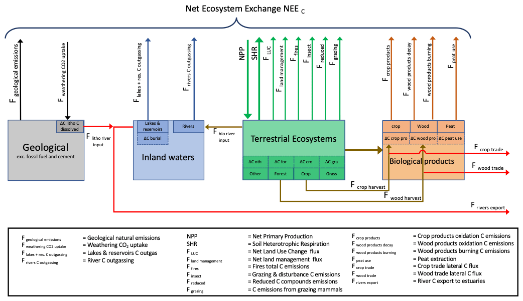
Figure 2 Summary of C fluxes to be reported in each RECCAP2 region (top) and the name of each flux (bottom).

The general recommendation is to provide, where possible, several estimates for each C flux based on different approaches. This could take the form of ensemble medians and ranges from different models. In the case where one estimate is thought to be more realistic than others, for instance a model with a better score when benchmarked against observations or a higher spatial resolution dataset with better ground validation, the underlying reasons for preferring that estimate need to be explained based on peer-reviewed literature or evaluation. Uncertainty can be calculated from the spread of different estimates in those cases where the state of knowledge cannot establish that one estimate is better than another. The use of IPCC methods (Mastrandrea et al., 2011) and uncertainty language (http://climate.envsci.rutgers.edu/climdyn2013/IPCC/IPCC_WGI12-IPCCUncertaintyLanguage.pdf, last access: November 2021​​​​​​​) is recommended when different estimates of the same component C flux are available. If different estimates report their own uncertainty, either based on data or an evaluation of the method used, e.g., by performing sensitivity analysis through changing model parameters, input datasets, or randomly varying input data, this information should be used to evaluate consistency between estimates, given their uncertainties. It is recommended to use the word “uncertainty” when comparing different estimates and “error” for the difference between an estimate and true values. Because “truth” is unknown for component C fluxes at the scale of large regions, errors cannot be estimated in RECCAP2.

3.1 Net carbon stock change

The net carbon stock change of terrestrial ecosystems C pools in a region (ΔC in Fig. 2) can be obtained by repeated inventories of live biomass, litter (including dead biomass), soil carbon, and carbon stock change in wood and crop products. None of the RECCAP2 region has a complete gridded inventory of all carbon stocks and their change over time. Some regions, like North America, China, Europe, and Russia have forest biomass inventories that were established long ago by forest resource agencies (Goodale et al., 2002; Pan et al., 2011). A few countries, e.g., England and Wales (Bellamy et al., 2005) and France (Martin et al., 2011), have repeated soil C inventories that allow trends to be quantified. Other countries have one-off soil carbon inventories (e.g., US, Australia, Germany). Many regions are able to make estimates of carbon stocks in products from forestry, wood use, and crop production statistics.

For RECCAP2, we recommend that each region reports carbon stock changes in all the listed terrestrial ecosystem aggregated pools in Fig. 2, namely ΔC_forest, ΔC_croplands, ΔC_grasslands, and ΔC_others, and specify which sub-pools are include in each case. The sub-pools can include, but are not limited to, the following sources: biomass, litter and woody debris, and soil mineral and organic carbon. Where attribution of these pools or sub-pools to biomes, land cover types, or political units is made by a regional synthesis group, the corresponding areas involved must be systematically reported. This includes the definition of the reporting depth for soil C stocks (0–30 and 0–100 cm are recommended). The choice of how many biomes are reported needs to balance data availability with the importance of carbon stock and carbon stock changes within particular biomes (typically a reported biome should contribute at least 10 % of the regional C changes). Regions with significant wetland C or permafrost C stocks may report this C stock separately, especially in cases where the areas involved occur in different biomes, but this must be done in a way that allows the C stocks to be subtracted from the biome total or added back into it without double counting. The area of biomes for which no carbon storage or carbon storage change is available needs to be reported, and a default value of −9999 should be given to such stocks and their stock change value. The biomes with no data can be specified (preferable if the area and stock involved is potentially large, since this identifies gaps needing future work) or simply lumped under “others” if they are minor.

The net C stock change of biological product pools also needs to be reported for crops, wood, and other carbon-containing products (see Fig. 2). The depletion of peat C stocks for use as a fuel (ΔC_{peat use} in Fig. 2), thus causing C emissions to the atmosphere, was significant in the early 20th century in some northern countries and still is today in few countries (Conchedda and Tubiello, 2020). It should be reported where relevant using regional data if available (Joosten, 2009). In the case of C stock change in wood products (ΔC_{wood products}), if possible the change in those wood products in use (e.g., construction, paper) should be reported separately from those in waste undergoing decay (e.g., landfills). The names and definitions of the wood product pools considered should be specified. The C stock change of crop product pools (ΔC_{crop products}) is usually small on an annual timescale. It can be reported if data are available, otherwise a value of zero can be assumed. The net carbon stock change of organic carbon accumulation in lakes and reservoirs (known as burial ΔC_burial) should be reported based on regional data or global estimates (Mendonça et al., 2017; Maavara et al., 2017).

3.2 Lateral displacement fluxes within and between regions

One of the reasons why net land–atmosphere C exchange that excludes fossil fuel emissions, hereafter called net ecosystem exchange (NEE), of a region is not equal to the net carbon stock change in the same region is because of lateral C fluxes, as alluded to in Sect. 1.5. Carbon is lost by each region to the adjacent estuaries through river export and is lost or gained through the trade of crop, wood, and animal products and through the atmospheric transport and deposition of C particles emitted with dust in dry regions. In order to allow the net C stock change estimates to be corrected, we recommend that lateral fluxes in and out of each RECCAP2 region be reported. The main ones are river C export and those from wood and crop trade, as denoted by the red arrows in Fig. 2. A strong point of the RECCAP2 project is an attempt at mass balance closure between pools and fluxes. Therefore, lateral displacement fluxes of C within each region but between pools denoted by the brown arrows in Fig.  should also be reported or calculated by mass balance. More details on these fluxes is given below.

3.2.1 Riverine carbon export to estuaries and the coastal ocean

Lateral C export fluxes in rivers (F_rivers in Fig. 2) should be reported at the interface between rivers and estuaries. We recommend to top the “land” at the mouth of rivers and to take estuaries being coupled to the coastal ocean by dynamical and biogeochemical processes as “blue carbon” in RECCAP2. Mangroves and salt marshes export large fluxes of dissolved and particulate C produced in upland systems or within riverine systems to estuaries and the coastal ocean (Bauer et al., 2013). These fluxes determine the carbon budget of the aquatic coastal margin ecosystems, and we recommend that they should also be considered “blue carbon”. River C fluxes at the river mouth into estuaries can be estimated from dissolved organic carbon (DOC), dissolved inorganic carbon (DIC), and particulate organic carbon (POC) concentration data for the rivers involved and the associated river flow rates (Ludwig et al., 1998; Mayorga et al., 2010; Dai et al., 2012). Few RECCAP2 regions (Fig. 1) receive C from rivers entering their territory. If this is the case, this input of flux of fluvial carbon from rivers should be reported, even though it is not represented in Fig. 2 for simplicity. Evasion from aquatic systems to the atmosphere is treated in Sect. 2.2.7.

3.2.2 Inputs of carbon to riverine from soils and weathered rocks

The inland water carbon cycle receives C leached or eroded from soils as an input. This carbon can be redeposited and buried in the freshwater ecosystems, outgassed to the atmosphere, or exported to estuaries and the coastal ocean. This flux is called F_{bio river input} in Fig. 2. It cannot be measured directly at large spatial scales. We therefore recommend calculating it by using mass balance as the sum of burial, outgassing, and export. Similarly, weathering processes consume atmospheric CO₂ (see Sect. 2.7). This C is subsequently delivered as dissolved bicarbonate ions to rivers. At the global scale and over long timescales, two-thirds of the average proportion of bicarbonate in waters is derived from atmospheric C with the final third being from lithogenic C. We recommend calculating this weathering-related DIC flux, called F_{litho river input} in Fig. 2, by using geological maps and global weathering rates (Hartmann et al., 2009).

3.2.3 Carbon fluxes in and out each region due to trade

Net trade-related C fluxes for wood and crop products exchanged by each region with other regions need to be reported in C units using statistical economic data about the trade volume and the carbon content of each product. These are available from regional datasets (or using FAOSTAT and GTAP data) or the global dataset of Peters et al. (2012). This net trade flux should be reported separately for crop products and wood products (F_{crop trade} and F_{wood trade} in Fig. 2). If the amount is relevant, it can be reported for animal products as well, but this flux is much smaller than that in crops and wood and is therefore not shown in Fig. 2. Our best-practice recommendation is to separate the net trade C flux into gross fluxes of imports and exports. The list of commodities included and ignored should be specified where they are material; commodities making a small contribution can be lumped under “other”. Quantification of carbon fluxes due to trade of unburned fossil fuels can be reported if data are available.

3.2.4 Crop and wood product transfers within in each region

Figure 2 links the C stock change of terrestrial ecosystem pools to the change of C storage in biological wood products by the harvest and lateral displacement of crop and wood. The harvest of grass for foraging can be assumed to be given to animals locally and can be included in F_grazing (see details in Sect. 2.4). We recommend reporting the total amount of C harvested as wood and crops in each region as F_{wood harvest} and F_{crop harvest} (Fig. 2), respectively. Subtracting trade fluxes from the harvest fluxes will provide the C flux displaced within each region for domestic activities. Note that non-harvested and non-burned residues for crops and forest harvesting, such as slash and felling losses, should not be part of the harvest flux and should instead be counted as part of F_LUC and F_{land management}. We note that this locally decomposing flux is globally large, in the year 2000 it amounted to 1.5 PgC yr⁻¹ for crop residues and 0.7 PgC yr⁻¹ for felling losses in forests (Krausmann et al., 2013).

3.3 Net ecosystem exchange

More than a decade ago there were a number of papers trying to reconcile different definitions of land carbon fluxes, including the papers by Schulze et al. (2000), Randerson et al. (2002), and Chapin et al. (2006). Schulze et al. (2000) focused on the importance of accounting for disturbance C losses at site scale when considering an ecosystem over a long time period and hence separating net ecosystem production (NEP, i.e., gross primary productivity minus ecosystem respiration) from net biome production (NBP or net biome productivity, i.e., NEP minus disturbance emissions). Randerson et al. (2002) argued that the net carbon balance should be described by a single name, NEP, provided that this flux includes all carbon gains and losses at the spatial scale considered. Finally, Chapin et al. (2006) in a “reconciliation” paper proposed the use of net ecosystem carbon balance (NECB) for the net C balance of ecosystems at any given spatial or temporal scale and the restriction of the use of NEP to the difference between gross primary productivity minus ecosystem respiration. These three definitions consider the C balance from the point of view of ecosystems. Here we seek to estimate the atmospheric C balance of ecosystems at the spatial scale of large regions and the temporal scale of 1 decade, and we call this net ecosystem exchange (NEE). NEE is defined as the exchange of all C atoms between a land region and the atmosphere over it, excluding fossil fuels and cement production emissions. We use a similar definition to Hayes and Turner (2012), but extend it to include natural geological emissions and sinks, acknowledging that geological fluxes are not from ecosystems per se. NEE includes biogenic atmospheric emissions of CO, CH₄, and VOCs, all expressed in C units. This definition of NEE matches the land–atmosphere flux of total C that inversions estimate, provided they account for CO₂, CH₄, CO, and VOC fluxes. NEE cannot be derived using the bottom-up approach from a single observation-based approach.

We acknowledge that the geological fluxes are not strictly speaking from ecosystems, and we could therefore have called this flux net terrestrial carbon exchange rather than NEE, but the former terminology could be ambiguous since some might assume that it includes fossil fuels and cement. NEE also includes biogenic emissions of CO, CH₄, and VOCs, all expressed in C units. This definition of NEE matches the land–atmosphere flux of total C that inversions estimate, provided they account for CO₂, CH₄, CO, and VOC fluxes. NEE cannot be derived using the bottom-up approach from a single observation-based approach. Various bottom-up datasets and methods must be combined to obtain each component flux, and those fluxes can be summed up to NEE.

We recommend that when a component C flux of NEE contains meaningful amounts of C emitted as CO, CH₄, and VOCs, the type and fraction of reduced carbon compound emitted should be reported. For instance, F_grazing emits carbon partly as CH₄; F_fires emits CO (and a smaller component of CH₄), VOCs, and CH₄; F_{wood products} emits CO when burned and CH₄ when the products decay in landfills (see Sect. 2.5); F_{rivers outgas}, F_{lakes outgas}, and F_{estuaries outgas} emit CH₄ (see Sect. 2.6); and F_{geological emissions} emit CH₄ and CO₂ (see Sect. 2.7). The CO₂ and reduced C composition of each flux should be reported separately for clarity, with both expressed in C units. This level of detail in the reporting will allow a precise comparison with inversion fluxes (see Sect. 1).

In Fig. 2, the component fluxes that sum to NEE are subdivided for four sub-systems: terrestrial ecosystems, biological products, inland waters, and geological pools (excluding those mined for fossil fuel and cement production). The section below describes the C flux components of NEE in each sub-system.

3.4 Component fluxes of net ecosystem exchange for terrestrial ecosystems

3.4.1 Net primary productivity

Net primary productivity (NPP) is the flux of carbon transformed into biomass tissues after fixation by GPP. In RECCAP-2 we recommend reporting GPP but focus on NPP as the relevant input flux of carbon to terrestrial systems. NPP can be measured in the field using biometric methods, but this method does not measure non-structural carbohydrates or NPP-acquired carbon lost to exudates, herbivores, leaf DOC leaching, biogenic VOC emissions, and CH₄ emission by plants (Barba et al., 2019). Field measurements thus estimate the biomass production (BPE is the sum of carbon in leaves, wood, and roots), which is lower than NPP. Different satellite products provide global maps of NPP for the past decades, but the conversion of GPP to NPP is usually made by an empirical carbon use efficiency model (ratio of GPP to NPP) like the BIOME-BGC model for the GIMMS-NPP (Smith et al., 2016) and for MODIS-NPP (Running et al., 2004) or the BETHY-DLR (Wißkirchen et al., 2013​​​​​​​​​​​​​​) global products. Field estimates of BPE can also be combined with satellite products of GPP to derive NPP (Carvalhais et al., 2014). Discussing uncertainties of satellite NPP and GPP products is not in the scope of this report, but light use efficiency formulations used in many datasets tend to ignore the effect of CO₂ fertilization and soil moisture deficits, which has motivated attempts to use data-driven models or hybrid models combining process-based leaf-scale photosynthesis models with satellite data, e.g., FAPAR, like in the P-MODEL (Stocker et al., 2019) or the BESS model for GPP (Jiang and Ryu, 2016). Those models assimilate satellite observations but include the effects of CO₂, diffuse light, or water stress on photosynthesis.

Additional methods can be used to estimate regional NPP. For crop NPP, aggregated estimates can be obtained from yield statistics and allometric expansion factors (Wolf et al., 2011), the spatial scale being the one at which yield data can be collected (e.g., farm, county, province, country). For forest NPP, woody NPP can be obtained from forest inventories, with some of the sites having several decades of measurements to enable studies of trends. The recommendation for RECCAP2 is to document the definition of NPP in the datasets that will be used for each region and the ecosystems covered in the case of NPP estimates limited to specific ecosystems as precisely as possible . It also needs to be made explicit how NPP datasets were obtained and what their possible limitations are. We recommend that NPP (rather than GPP) should be reported for each region, given that C from NPP links directly to biomass and soil C inputs and to partial appropriation by humans and animals in managed ecosystems, due to the fact that harvested C is further displaced laterally and turned into emissions of C to the atmosphere where it is used.

3.4.2 Carbon emissions from soil heterotrophic respiration (SHR)

Soil heterotrophic respiration (SHR) is the C emitted by decomposers in soils and released to the atmosphere. Up until recently, this flux could not be estimated directly, but the availability of point-scale measurements from 6000 sites for total soil respiration and ≈500 sites for heterotrophic respiration in the peer-reviewed literature used by the SRDB 4.0 database (Bond-Lamberty, 2018) allows for regional and global upscaling of this flux for averages over a given period (Hashimoto et al., 2015; Konings et al., 2019; Warner et al., 2019) or with annual variations (Yao et al., 2021) that can be used for RECCAP2.

3.4.3 Carbon fluxes from land use change and land management

The net land use change flux, called F_LUC, includes C gross fluxes exchanged with the atmosphere from gross deforestation, legacy and instantaneous soil CO₂ emissions, forest degradation emissions, and sinks from post-abandonment regrowth and afforestation and reforestation activities (Houghton et al., 2012). This flux can be positive or negative depending on the region considered and the balance of gross fluxes. The net land use change flux results from changes in NPP, SHR, and deforestation fires over areas affected by land use change in the past. Attribution by cause is, in this case, relevant to evaluate the human impact on terrestrial CO₂ exchange and to inform policy making. In absence of local NPP and SHR measurements over areas subject to land use change, especially at the scale of RECCAP-2 regions, F_LUC should be treated as a separate flux component of NEE in each region. F_LUC is widespread in all RECCAP2 regions and highly uncertain, and its estimates depend on the approach used. The different terms and definitions used to estimate F_LUC need to be clearly defined to avoid counting the fluxes twice within the regional budgets. More details about the calculation of F_LUC are given in Sect. 4 since estimates depend on the method used.

The carbon flux exchanged with the atmosphere from management processes, called F_management, includes a wide range of forest, crop, and rangeland management practices. It is extremely difficult to separate F_management from F_LUC as it would require the quantification of C fluxes from land use change, followed by no management of the new land use in F_LUC and C fluxes from additional management activities on top of land use change. In practice, bookkeeping models of F_LUC include management of new land use types in the empirical data they use. Fire is also commonly used in land management and for deforestation, but it is only implicitly included in F_LUC estimates. For instance, forest to cropland land use emissions are based on empirical observations of soil C changes in croplands from multiple sites, which implicitly include tillage, fertilization, cultivars, and biomass burning effects but do not separate each of these practices explicitly in each region due to a lack of data.

Likewise, F_management is not simulated separately in global studies based on dynamic global vegetation models (DGVMs), and the effects of management are included in F_LUC instead, based on the idealized parameterizations of management practices (Arneth et al., 2017). For croplands, DGVMs include crop harvest preventing the return of residues to soils, and some models represent tillage (Lutz et al., 2019) and changes in fertilization (Olin et al., 2015). To our knowledge, there is no DGVM simulating the effect of irrigation, changes of cultivars and rotations (cover crops), and conservation agriculture on C fluxes. For fires, management activities such as deforestation fires or fire prevention are usually not represented, although population density maps are used to modulate ignitions. For managed forests, several global models that include wood harvest (Arneth et al., 2017; Yue et al., 2018) as a forcing do not have a detailed representation of practices, mainly due to the lack of forcing data, although management is represented in some regions (Luyssaert et al., 2018). For pastures, few models include variable grazing intensity, fertilization, and forage cutting (Chang et al., 2015). In addition to structural DGVM limitations and a lack of representation of management precluding an estimate of F_management, there is also no framework to perform factorial simulations with and without land use change and management that would allow us to separate F_management and F_LUC.

F_LUC and F_management are accounted for by UNFCCC national communications of C fluxes in the land use, land use change, and forestry (LULUCF) sector for managed lands. UNFCCC national communications report land use change emissions in their Common Reporting Format (CRF) communications for different bidirectional land use transitions. These estimates of F_LUC have a different system boundary from those simulated by bookkeeping models (Grassi et al., 2018; Hansis et al., 2015; Houghton and Nassikas, 2017). National communications following the IPCC guidelines (Dong et al., 2006) usually do not consider F_LUC from land use that occurred more than 20 years before the reporting period, whereas bookkeeping models and DGVMs consider all land use transitions that occurred since 1700 CE. On the other hand, national communications include F_LUC from the expansion of urban areas, which is ignored in bookkeeping models and DGVMs. In national communications, F_management as defined here is not separately estimated. Its effect is implicitly included in the LULUCF sector based on empirical emission factors that include management practices of the new land use types in reports of C fluxes of stable land use types (e.g., cropland remaining croplands). Since 75 % of the global land ecosystems are managed (Ellis et al., 2010; Liang et al., 2016), it will be a major challenge for RECCAP2 to comprehensively account for F_LUC and F_management and even more challenging to reach a harmonized method for comparing estimates between regions. We thus recommend for each synthesis chapter to describe the components of F_LUC and F_management as precisely as possible and to explain in which cases they are combined together. Note that it is recommended that the emissions of wood products, crop products, and grazing are reported as separate fluxes. If they are provided as part of F_LUC and F_management they should thus be identified separately.

3.4.4 Carbon emissions from fires

This flux, called F_fires, represents the emission of all carbon species to the atmosphere from wildfires, prescribed fires, biomass burning, and biofuel burning, including CO₂, CO, CH₄, and black carbon, separated if possible into crop residue burning and other fires. The burning of crop residues occurs though small-scale fires, which continue to be underestimated by global satellite burned area products. Further, some residues are burned out of the field, and those emissions are not measurable with satellites. Burning emissions from crop residues can be calculated from fuel consumption and carbon emission factors. Emissions from other fires can be estimated by ground-based and aerial surveys (several countries perform such surveys) or from satellite-based datasets based on burned areas, such as GFED (van der Werf et al., 2010) (https://www.globalfiredata.org, last access: November 2021​​​​​​​), or based on fire radiative power, such as GFAS (Di Giuseppe et al., 2018). The Global Fire Emission Database version 4.1s (GFED4.1s) is an update of the GFED3 product with an updated burned area and is complemented by an active fire detection algorithm that improves detection of small fires (van der Werf et al., 2017). In tropical regions, deforestation causes fires (including peat fires in Southeast Asia). It is important here to avoid double accounting by checking in each region if C emissions from deforestation fires were already included in land use change emissions (F_LUC), and if this is the case these must be subtracted from F_fires. A possible approach here is to separate fire emissions over intact, transitional, and managed lands if spatially explicit datasets for managed lands are available (Table 1).

Table 1 Cross-cutting processes in carbon budgets and their separation by cause in different approaches.

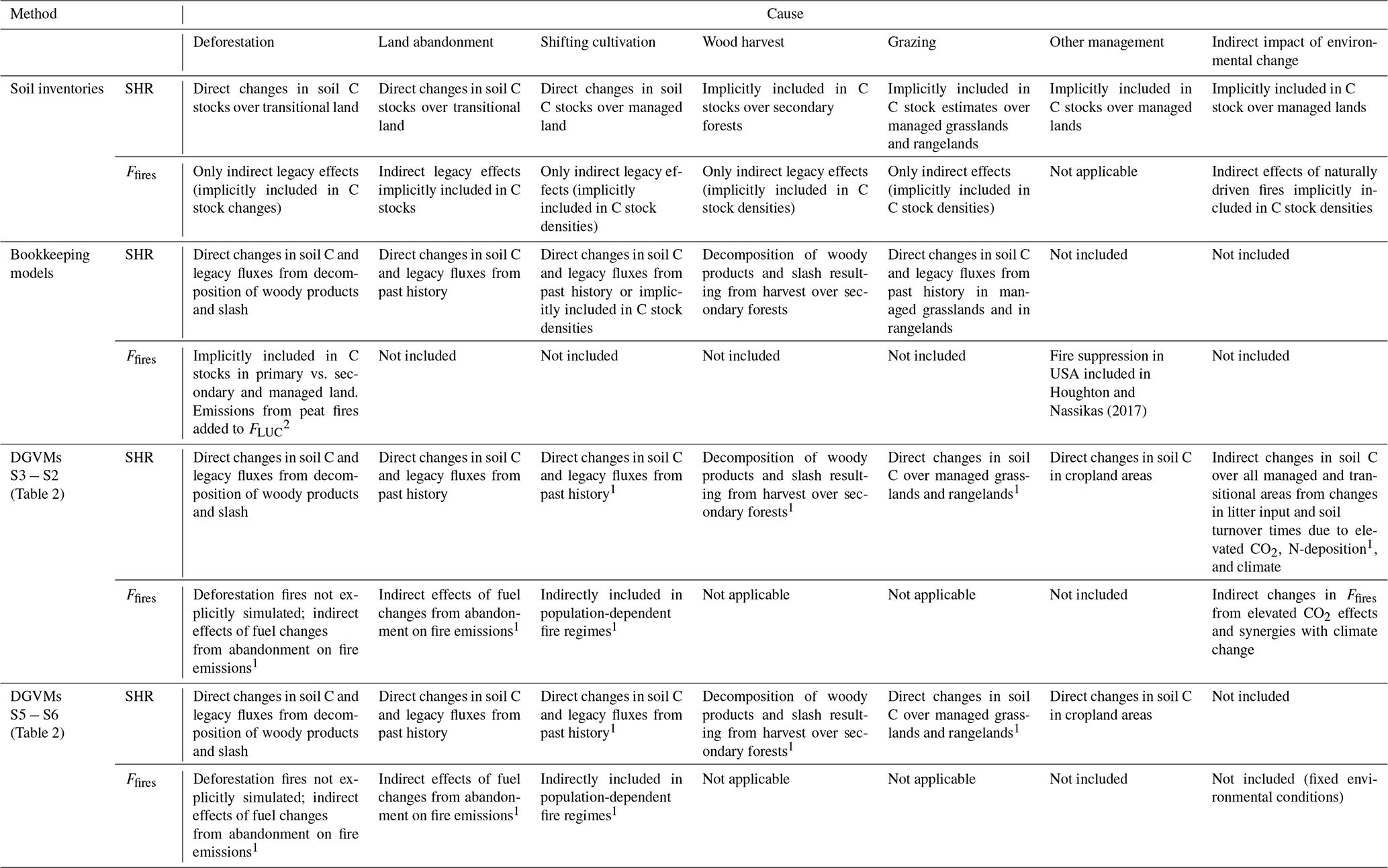
¹ If simulated by individual DGVMs. ² In Houghton and Nassikas (2017) and BLUE (Hansis et al., 2015) models.

3.4.5 Carbon emissions from insects grazing and disturbances

This flux, called F_insects, represents C emissions to the atmosphere associated with background grazing and sporadic outbreak of insects. It is a significant C emission in regional budgets, though it is usually ignored, but it may be estimated as a fraction of NPP or leaf biomass if data is available and provided there is no double counting. Insect outbreaks (Kautz et al., 2017) cause direct and committed emissions to the atmosphere beyond the background grazing of a fraction of biomass as they partly destroy foliage or cause tree morality (e.g., bark beetles in Canada, Kurz et al., 2008) that induces legacy emissions that can last for several decades. To our knowledge, only a few regions have estimates of insects-disturbance-induced C emissions at a regional scale, e.g., the US (Williams et al., 2016), Canada, and some countries in Europe, and this component flux may not be possible to estimate for each RECCAP2 region (particularly in tropical regions).

3.4.6 Carbon emissions from reduced carbon species

This flux, called F_reduced, is the sum of emissions to the atmosphere of reduced C compounds, including biogenic CH₄, non-methane biogenic volatile organic compounds (BVOCs), and biogenic CO (excluding fires). Carbon emitted as CH₄ by wetlands, termites, and rice paddy agriculture sources and removed by soils can be estimated by bottom-up approaches, e.g., synthesized in the global CH₄ budget or from atmospheric CH₄ inversions in the case where those inversions report those flux components separately (Saunois et al., 2020). In the framework proposed here, CH₄ emissions from crop and wood products in landfills are counted as F_{crop products} and F_{wood products}, and CH₄ carbon from animals and manure is counted in F_grazing. Emissions of carbon from BVOCs and CO by the vegetation can be obtained from models used to simulate those fluxes for atmospheric chemistry after conversion into units of carbon mass. For instance, the CLM-MEGAN2.1 model (Guenther et al., 2012) estimates biogenic emissions of CO and of ∼150 BVOC compounds, with the main contributions being from terpenes, isoprene, methanol, ethanol, acetaldehyde, acetone, α-pinene, β-pinene, t-β-ocimene, limonene, ethene, and propene.

3.4.7 Carbon emissions from biomass grazed by animals

This flux, called F_grazing, represents the C emission that incurs from the consumption of herbage by grazing animals, including the decomposition of animal products used in the bio-economy, the decomposition of manure, and direct animal emissions from digestion. Only the fraction of manure from animals grazing on grass should be accounted for because C emitted from manure originating from crop products given to animals is already included inF_{crop products}. Grass requirements by animals can be derived from grass biomass use datasets (Herrero et al., 2013). Grass biomass use per grazing animal head in a region can be calculated based on data of total metabolizable energy (ME) of ruminants in each region. Actual grass intake can be derived from empirical models or from vegetation models that include management of pasture (Chang et al., 2016). Carbon emitted from grazed grass biomass includes CH₄ emissions from manure C (excreta) and from enteric fermentation, animal CO₂ respiration from grass intake, and C emissions from the consumption and decay of meat and milk products derived from grass grazing. The C in milk, animal, and manure products can be assumed to decay in 1 year and to be emitted as C to the atmosphere. Here “animals” are domestic or wild mammals but not insects.

3.5 Component fluxes of net ecosystem exchange from biological products

3.5.1 Carbon emissions from crop biomass consumed by animals and humans

This flux, called F_{crop products}, represents the carbon emissions to the atmosphere from the consumption of harvested crop products. It can be calculated from agricultural statistics as the sum of domestically harvested products minus net export minus storage in each region. Crop products are consumed both by animals (including wild animals) and humans, and a distinction may be made between these two groups of consumers if additional data on consumption type are available in each region. The digestion of crop products by ruminants emits CH₄ carbon and double-counting must be avoided in case this CH₄ and C flux is included in another C flux like ruminant methane emissions. A fraction of C in consumed crop products is also channeled to sewage systems and lost to rivers as DOC instead of being emitted to the atmosphere (globally 0.1 PgC yr⁻¹; Regnier et al., 2013). Although it is a small flux, we recommend including it in regional budgets if data are available. River CO₂ outgassing flux estimates should contain the fraction of this sewage C flux returned back to the atmosphere.

3.5.2 Carbon emissions from harvested wood products used by humans

This flux, called F_{wood products decay}, represents a net carbon emission to the atmosphere from the decay and burning of harvested wood products used for paper, furniture, and construction. The emission from decay, F_{wood products decay}, can be calculated with models of the fate of wood products in the economy, e.g., Eggers (2002), Mason Earles et al. (2012), forced by input to product pools from domestic harvest of non-fuel wood and net export of wood products. The small fraction of wood product waste going to sewage waters and rivers can also be estimated if relevant data are available. If F_{wood products decay} is calculated in carbon units, e.g., from a model of wood product pools, it also includes carbon lost to the atmosphere as CH₄ in landfills, thus double-counting must be avoided in case CH₄ and C emissions from wood in landfills are also reported separately in a region. The flux from burning of wood products, F_{wood product burning}, can be estimated from statistics of fuel wood consumption and carbon emission factors during combustion (including CO₂, CO, and CH₄). This flux should include emissions from commercial fuel wood burned to produce electricity, non-commercial fuel wood gathered locally and burned in households, and fuel wood burned as a fuel by industry. It is important to note that we recommend to report F_{wood products decay} here for each RECCAP2 region as a separate flux. This term is usually included in F_LUC in C budget studies based on DGVMs and bookkeeping models (Friedlingstein et al., 2019). It should then be removed from currently reported estimates of F_LUC in order to avoid double-counting.

3.6 Component fluxes of net ecosystem exchange for inland waters

Carbon emissions from rivers, lakes, and reservoirs

The​​​​​​​ fluxes, called F_{rivers outgas} and flakes plus reservoirs outgas in Fig. 2, correspond to those from the outgassing of C from lakes and rivers, respectively. There are two global observation-based estimates of this flux calculated using the same GLORICH river pCO₂ database but with different data selection criteria and upscaling techniques. That of Raymond et al. (2013) was produced using the COSCAT regions that represent groups of watersheds and can be re-interpolated to the RECCAP2 regions. That of Lauerwald et al. (2015) was produced on a 0.5^∘ × 0.5^∘ global grid and does not include lakes. Gridded CO₂ emissions of boreal lakes have been estimated separately by Hastie et al. (2018) using an empirical model trained on pCO₂ data from mainly Swedish and Canadian lakes. The riverine CO₂ evasion outgassing flux from Lauerwald et al. (2015) is about half that of Raymond et al. (2013) due to lower estimates of average river pCO₂ for the tropics and Siberia resulting from a more restrictive data selection process and additional averaging effects from the statistical model applied. In addition, the estimates by Lauerwald et al. (2015) do not account for CO₂ emissions from headwater streams, which may be substantial. For instance, Horgby et al. (2019) estimated that mountain streams alone emit about 0.15 PgC yr⁻¹ globally. Some land models have been developed to include the land to ocean loop of the carbon cycle, and their output may be used to assess river and lake CO₂ evasion fluxes for selected regions (Hastie et al., 2019) or the globe. These models have also confirmed previous observational findings (e.g., Borges et al., 2015) that river floodplains are a potentially significant yet overlooked component of the inland water C budget. Up until now, however, only CO₂ outgassing from rivers, lakes, and reservoirs has been considered in regional C budgets. New synthesis estimates of CH₄ emissions from those inland waters are now available from the CH₄ budget synthesis (Saunois et al., 2020), and we recommend that this source in C units should be added to F_{rivers outgas} and F_{lakes+reservoirs outgas}.

3.7 Component fluxes of net ecosystem exchange from geological pools

3.7.1 Geological carbon emissions

This flux, called F_{geological emissions}, corresponds to natural emissions of CO₂ and CH₄ from geological pools. The Earth's degassing of geological carbon consists of geogenic CO₂ emissions of 0.16 PgC yr⁻¹ (Mörner and Etiope, 2002), microbial oxidation of rock carbon (Hemingway et al., 2018), and CH₄ emission estimated to be 0.027 PgC yr⁻¹ (Etiope et al., 2019), which has recently been revised (Hmiel et al., 2020) to a smaller value of 0.0012 PgC yr⁻¹. Geogenic CH₄ and C land emissions are from volcanoes, mud volcanoes, geothermal sources, seeps, and micro-seepage, and if the gridded dataset of Etiope et al. (2019) is used, we recommend removing the marine coastal seepage CH₄ and C emissions reported separately in this dataset. Geogenic CO₂ and C emissions are almost exclusively related to geothermal and volcanic areas (high-temperature fluid–rock interactions, crustal magma, and mantle degassing). We suggest here to report these fluxes if there is a published estimate in the region considered.

3.7.2 Weathering uptake of atmospheric CO₂

This flux, called F_{weathering uptake}, corresponds to the weathering of carbonate and silicate rocks, which is a net sink of atmospheric CO₂ and corresponds to C then transferred by rivers to the ocean. We recommend that these fluxes should be reported for each region as they are needed to rigorously compare the output of CO₂ inversions (which cover all CO₂ fluxes) with bottom-up NEE estimates (Fig. 2). This can be achieved using the global dataset from Hartmann et al. (2009) and the gridded product of Lacroix et al. (2020) for instance. Weathering of cement is represented in Fig. 2 and should be reported as part of fossil fuel emissions, which is not within the scope of this paper.

4 Methods to estimate bottom-up components of NEE

The methods described here are as follows:

• C stock changes from ground-based estimates (forest biomass and soil carbon inventories),

• CO₂ fluxes measured by eddy covariance,

• other ground-based measurements (e.g., pCO₂ in rivers, site NPP, soil respiration data),

• models driven by statistical data (e.g., wood and crop products and grazing emissions),

• models driven by satellite data (e.g., fire emissions models, NPP models),

• process-based terrestrial carbon cycle models (e.g., TRENDY models).

The general approach of RECCAP2 is to use more than one of these approaches for each flux to gain further insights into the carbon budget of a region by exploring the full range of data available. The purpose of this section is to describe what each method does and does not estimate in terms of NEE component C fluxes, as defined in Sect. 2 and illustrated in Fig. 2, and therefore what valid comparisons can be made.

4.1 Inventory-based measurements of carbon stock changes

This approach generally uses biomass determined from repeated forest inventories. The stock changes for the LULUCF sector in UNFCCC communications reports are usually based on inventories. In some countries these have been done for many years, but in many countries they are not available. The sampling density and sampling schemes vary greatly between countries and regions (Pan et al., 2011). The Global Forest Biomass Biodiversity Initiative (https://www.gfbinitiative.org, last access: November 2021​​​​​​​) contains 1.2 million forest plots, mainly in countries in the Northern Hemisphere, although the data are currently not publicly available. The forest inventory data for tropical regions typically comes from research plots, rather than production forests. Forest inventories measure aboveground biomass, from which C stocks can be derived (and stock changes in case of repeated census), but do not quantify soil carbon changes. Repeated inventories of soil carbon only exist in very few countries or regions; where they do, they are often focused on agricultural soils alone. If site history information is available, the repeated inventories of biomass and soil C can be used to F_LUC over time for various land practices.

Point-scale data from inventories can be upscaled (by simple averaging, by including spatial trends and covariates using geo-statistics, or more recently by using machine learning) to provide regional budgets of C stock changes in biomass and soils. Forest biomass inventory estimates of tree mortality can further be used to estimate C stock changes for pools that are not directly measured, like litter and soil C, given assumptions regarding their mean residence times. For instance, in their global synthesis of forest C stock changes, Pan et al. (2011) used simple fractions of growing stocks to estimate soil carbon changes. In national inventories, more detailed models of soil C change can be used.

C stock changes are assumed to be the sum of NEE and lateral C fluxes exported from or imported into the territory considered. For RECCAP2, this territory is the area of each region, where the lateral fluxes consist of C exported to the ocean via inland waters and exported or imported from trade routes, as it is impractical to have observation-based gridded datasets of lateral fluxes at sub-regional resolution. Therefore, when comparing observation-based C stock change estimates with independent NEE estimates, e.g., from inversions or other sources, it is strongly recommended to first correct the stock change from each region by the net import or export of C in trade and by the export in rivers. In RECCAP2, there is potential to use smaller sub-regions than in RECCAP1, and thus some regions may also receive incoming C from rivers entering their territory.

4.2 Eddy covariance networks

Eddy covariance flux tower networks measure the net CO₂ flux of terrestrial ecosystems (NPP-SHR) across a global network with a typical footprint of about 1 km². The networks currently consist of about 600 sites (Jung et al., 2020). Given the small footprint, flux tower sites do not adequately measure the fluxes of F_geological, F_fires, F_reduced, F_{rivers+lakes outgas} (except for a very few towers in wetlands or flooded systems), F_{crop products}, and F_{wood products}. For F_grazing, only the fraction emitted as CO₂ by livestock in the field (not in the barn) in the footprint of a tower is measured. Too few towers are installed over ecosystems in transition at different times after a land use change, and the network is potentially biased toward younger, more productive forest stands, and thus regional estimates of F_LUC cannot be directly obtained from eddy covariance flux towers measurements. The small spatial footprint of eddy flux towers can be upscaled into gridded maps of NPP-SHR (NEE at ecosystem level) using the relationship between the continuous measurements from flux towers and simultaneously recorded climate and vegetation parameters. The fluxes are upscaled using gridded predictors from remote sensing (such as FAPAR or NDVI) and climate fields using machine learning or data assimilation techniques (Jung et al., 2020; Tramontana et al., 2016).

Both inventories and eddy covariance networks provide point sampling with many gaps between points. These gaps are filled using upscaling models like FLUXCOM (Jung et al., 2020; Tramontana et al., 2016). The FLUXCOM data show fair agreement with inversions and TRENDY models for the seasonal cycle of NEE and for the phase of inter-annual NEE anomalies (Jung et al., 2017), but the absolute magnitude of interannual anomalies is strongly underestimated. One attempt to close the global NEE budget by combining FLUXCOM estimates of GPP and total ecosystem respiration (TER) with other fluxes not measured by flux towers (Zscheischler et al., 2017) obtained a net sink of CO₂ that was 10 PgC yr⁻¹ larger than the net land CO₂ sink deduced from the global budget. One possible reason for this mismatch could be biases introduced during the processing of micro-meteorological observations, for instance u^* filtering, or the sampling bias in the tower network. The tower sites are not randomly distributed, and therefore they measure fewer recently disturbed ecosystems (typically C sources) than recovering ones (C sinks), thus overestimating CO₂ uptake given the available network. Since we do not know the true distribution of land fluxes, upscaling models of flux towers data could miss important ecosystems not sampled by the training data or representative landscape elements with intense sources (peatlands, permafrost, disturbed ecosystems) or sinks (peatlands, plantations) that might contribute significantly to the carbon balance of a region.

We recommend that RECCAP2 teams use eddy covariance estimates of net ecosystem CO₂ fluxes, but since they consist only of NPP and SHR, these fluxes should add C fluxes not measured by this approach. This can be done using aggregated estimates of the non-measured C fluxes in each region or using gridded estimates. For instance, Zscheischler et al. (2017) used gridded estimates of F_fires, F_{rivers+lakes outgas}, F_LUC, F_{crop products}, and F_{wood products}. They did not add F_reduced, but gridded monthly estimates of this flux could be included in RECCAP2 based, e.g., on Guenther et al. (2012). We should remain cautious, noting that NPP and SHR upscaled from eddy flux towers so far gives unrealistically high global CO₂ sinks.

4.3 Other ground-based measurements

The list provided here is not exhaustive. It includes “ecological” measurements of NPP (e.g., Olson et al., 2001), biometric C stock changes at site level (e.g., Campioli et al., 2015; Luyssaert et al., 2007); soil respiration, e.g., the SRDB database (Bond-Lamberty and Thomson, 2010); and pCO₂ data in rivers and lakes (GLORICH). These measurements are sparse and local in nature. In a similar fashion to the flux tower measurements described above, it is possible to derive empirical relationships linking point data with local climate and other predictor variables; these relationships can then be used for spatial or temporal extrapolation using gridded fields of the same predictors. In recent years, gridded estimates have been provided for soil respiration (Hashimoto et al., 2015), soil heterotrophic respiration (Konings et al., 2019; Tang et al., 2020), and F_{river+lakes outgas} (Lauerwald et al., 2015; Raymond et al., 2014), which can be used to create regional totals.

4.4 Models driven by statistical data

Here we refer to a variety of models that do not use physical measurements at selected locations but instead use statistical data about harvested C, C in product pools, and C traded or consumed. These data are usually sourced from national or international statistical agencies or sector bodies. Examples are the study of Wolf et al. (2015), who estimated crop NPP, F_grazing, and F_{crop products}; Krausmann et al. (2013), who estimated crop NPP from statistical data on yield; Ciais et al. (2007), who estimated F_{crop products} and the corresponding CO₂ uptake by growing crops and horizontal displacement of harvested crop biomass; and Zscheischler et al. (2017), who provided gridded estimates of F_{wood products} (albeit ignoring trade).

4.5 Models driven by satellite data

Satellite data are also used in upscaling forest inventory, eddy covariance, and other ground-based measurements, although giving a full list of this category of models is not the purpose of this paper. Here we refer to satellite-driven NPP models (Bloom et al., 2016; Smith et al., 2016; Running et al., 2004; Tum et al., 2016; Wißkirchen et al., 2013) based on light use efficiency formulations or hybrid land carbon cycle models that explicitly represent photosynthesis (and NPP) driven by directly assimilated satellite data. Similarly, fire emission models like GFED and GFAS rely on satellite input data like burned area and fire radiative power (FRP) but estimate emissions using fields from models or other datasets (information on the fuel load, the burning completeness, and emission factors for different gaseous species). Remotely sensed models of aboveground biomass, derived from optical sensors, i.e., MODIS (Baccini et al., 2017), lidar from ICESAT-1 GLAS (Saatchi et al., 2011), synthetic aperture radar (SAR, Santoro, 2018), and L-band vegetation optical depth (VOD, Liu et al., 2015), have been produced globally and regionally (i.e., for mangroves using X-band radar, Simard et al., 2019). When they are repeated over time they allow estimates of biomass stock change, such as those presented by Brandt et al. (2018) over Africa and Fan et al. (2019) over the tropics. These datasets differ not only in their methodology and training datasets but also in their spatial (300 m to 25 km) and temporal (annual, or epoch) resolutions, and thus an ensemble-based approach is preferable for assessing uncertainty. Belowground carbon stock estimates are more challenging to access, and for live root biomass often a scaling assumption is made, but for mineral and organic carbon estimates are derived from the empirical upscaling or inventory approaches or process-based models described in Sect. 3.6.

4.6 Process-based terrestrial carbon cycle models

Dynamic global vegetation models (DGVM) simulate bottom-up NEE and a number of ecosystem carbon pools and fluxes, and their change over time on a gridded basis worldwide. The grid resolution ranges from 0.5^∘ for global applications, e.g., TRENDY (Sitch et al., 2015) or MstMIP (Wei et al., 2014), to fine resolutions (300 m or less) regionally. These models are not tightly driven by observations (unlike those in Sect. 3.5), but some observations are used by modelers to calibrate parameters. TRENDY models are now benchmarked following ILAMB (Friedlingstein et al., 2019). Dense observation datasets are not assimilated systematically, although some carbon cycle data assimilation systems exist that make use of DGVMs (Kaminski et al., 2013; MacBean et al., 2016) or simpler models like CARDAMOM (Bloom et al., 2016). The advantages of DGVMs for carbon budgeting are that (1) they provide an ensemble of gridded NEE and NEE component estimates as part of TRENDY and that (2) these models should in principle conserve mass and simulate consistent C fluxes and C stock changes for all regions. A limitation of DGVMs (apart from the fact that they can differ substantially from observations) is that they do not explicitly represent some of the fluxes in Fig. 2. F_fires is available from 10 out of 16 DGVMs in TRENDY and FIREMIP (Hantson et al., 2020). F_LUC from DGVMs includes a foregone sink of CO₂ called the loss of additional sink capacity (Gasser et al., 2020; Pongratz et al., 2014), which is not included in data-driven methods, to quantify this flux (see Sect. 4). DGVMs partly include F_{wood products} and F_{crop products} but assume that all harvest is released locally as CO₂ to the atmosphere, ignoring lateral displacement of harvested C within and across regions. DGVMs ignore F_reduced and only one or two include F_{rivers+lakes outgas}. Hence, care should be taken when combining DGVM outputs with observation-based estimates of C fluxes because of double-counting or undercounting. For instance, C outgassing from rivers and lakes derives from C exported by soils, but if this export is not represented in a DGVM, C will be otherwise released as SHR, and thus adding to DGVM output an outgassing flux would lead to an erroneous double-counting.

In general, for RECCAP2 we recommend describing exactly what each estimation approach includes or excludes for each C flux of Fig. 2 in order to minimize the risk of missing some fluxes or double-counting others. Mass conservation should be the key underlying principle when combining bottom-up C fluxes originating from different approaches.

5 Fluxes from land use change

Fluxes from land use change and management (abbreviated to F_LUC and defined as having a positive sign for net fluxes from the atmosphere to the land C) are defined as changes in C stocks due to deforestation, forest degradation and afforestation or reforestation, wood harvest, subsequent regrowth of forest following harvest or agriculture abandonment, conversion between croplands and grasslands (also sometimes called pastures or, more generally, rangelands), and management practices such as shifting cultivation (land cyclically rotating between forest and agriculture). Where applicable, peat burning and drainage should also be considered, as well as carbon fluxes related to management practices such as fire management, particularly if those practices have changed within the relevant period (for instance, when historically burning ecosystems are subject to fire suppression or where fire-protected ecosystems become fire-susceptible ecosystems) (Alvarado et al., 2020; Forkel et al., 2017; Kelley et al., 2019). Where possible, F_LUC should be separated into the component fluxes corresponding to the different processes and adding up to the net regional F_LUC. Typical components of F_LUC, as reported by bookkeeping models, include immediate biomass losses during deforestation, delayed emissions from soil carbon and litter decomposition for all subsequent years following land use change (legacy emissions), emissions from wood products harvested as a result of deforestation or derived from secondary forests, and recovery gains due to secondary forest regrowth or afforestation (Hansis et al., 2015; Houghton et al., 2012). Previous versions of the Houghton et al. (2012) bookkeeping model (up until 2017) reported emissions from shifting cultivation as part of F_LUC, but this term has been dropped in the most recent version of this model (Houghton and Nassikas, 2017). Houghton and Nassikas (2017) also provide emissions from forest degradation (i.e., biomass-reducing activities that do not result in the land parcel being reclassified as a non-forest) and subsequent recovery as part of F_LUC.

The various methods available to quantify F_LUC (Table 2) rely on different input datasets and models with different abilities to represent land use practices. They further use different terminology and assumptions of which component fluxes to include, leading to inconsistencies between one another. For RECCAP2, the best data available in each region should be used. However, it is crucial to clearly define the methods and assumptions made and which F_LUC fluxes are included in the corresponding results. If possible, regional F_LUC fluxes estimated by the “best method” should be compared with those estimated by the global datasets from the most up-to-date Global Carbon Budget coordinated by the Global Carbon Project (GCP) Global Carbon Budget in order to ensure consistency and comparability between regions. The methods used to estimate F_LUC include: (i) bookkeeping models (BKs), (ii) dynamic global vegetation models (DGVMs), (iii) remote-sensing based methods, and (iv) national inventories, as detailed below.

Table 2 Main differences between the methods used to estimate F_LUC.

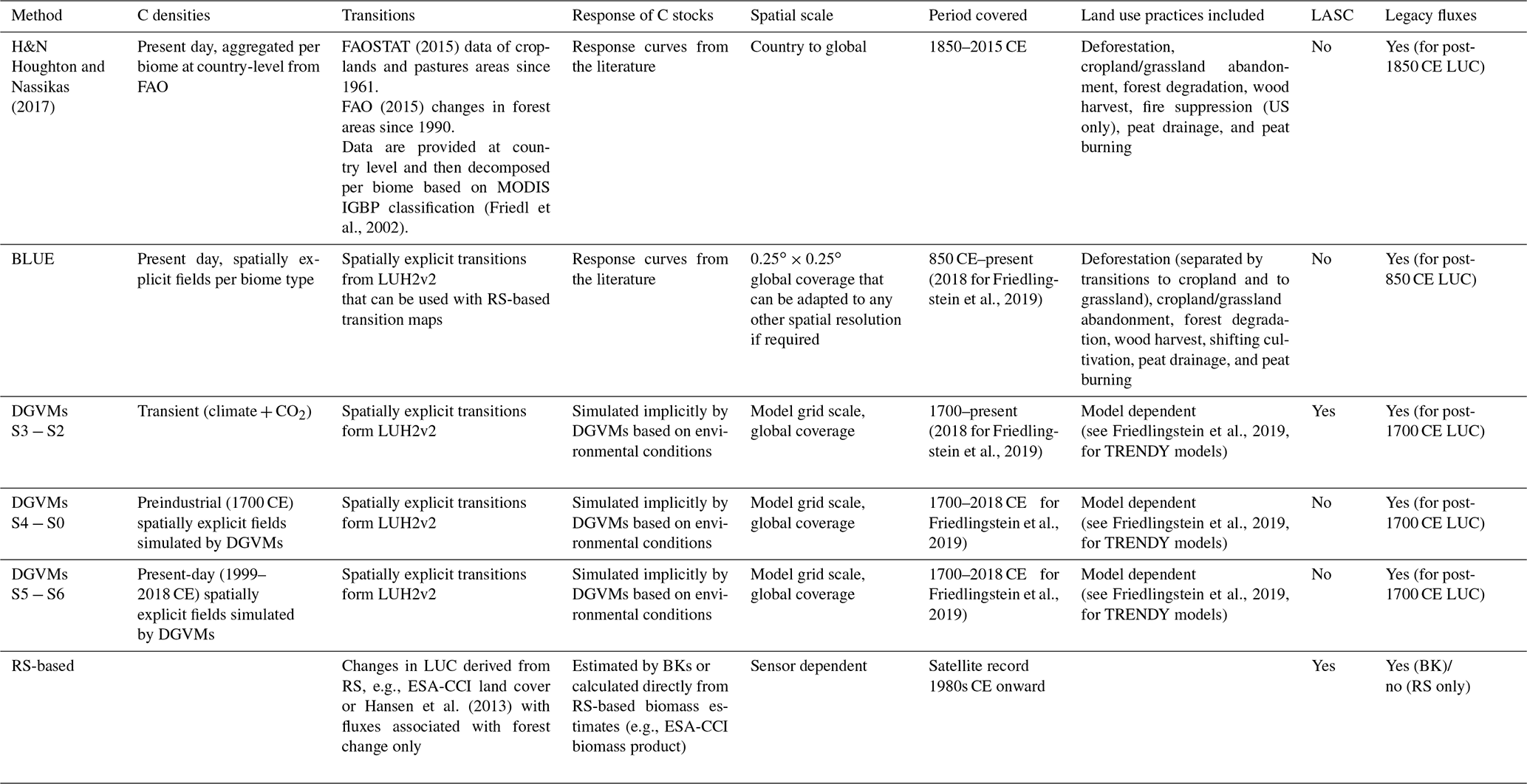
5.1 Bookkeeping models

Bookkeeping models rely on present-day vegetation and soil C densities (aggregated or spatially explicit) and different response curves (i.e., time courses of change) to estimate changes in C stocks following a given transition. F_LUC in bookkeeping models includes respiration fluxes from crop and wood harvest slash and from legacy fluxes due to land use change. Based on the underlying forcing data, these can be separated by cause (e.g., management, deforestation, land abandonment, shifting cultivation). The two BK models used in the Global Carbon Budget (GCB) (Friedlingstein et al., 2019) are those from Houghton and Nassikas (2017) and Hansis et al. (2015), referred to as H&N and BLUE respectively. Both BK models are able to provide F_LUC at country level but differ in a number of characteristics, such as the input data, the C densities and response curves used, the spatial resolution, and period covered, as summarized in Table 2. Spatially explicit BK models such as BLUE can be adapted to run at regional scales with finer spatial resolution of land use change, derived from either national inventories or from remote-sensing (RS)-based transitions (e.g., ESA-CCI land cover). If very good data on C densities and ideally response curves is available regionally and no superior regionally BK model is available, BLUE can also be adapted to run with that information at country or regional level. One term that is not considered by bookkeeping models is the indirect effect of climate and environmental variability and change on sinks and sources (including respiration fluxes) resulting from land use change (LUC) (Obermeier et al., 2021; Yue et al., 2018). This effect is, however, implicitly included in stock-change-based estimates used in national inventories and in the most commonly used method to estimate F_LUC by dynamic global vegetation models. Below, we discuss how to reconcile these different estimates.

5.2 Dynamic global vegetation models (DGVMs)

DGVMs explicitly simulate the processes controlling photosynthesis, growth, decomposition, and mortality of vegetation and the processes involved in biomass and soil C changes. They also simulate the fluxes resulting from forest clearing, pasture and crop conversion, abandonment and regrowth, and crop harvest, although the implementation varies between models, as do the assumptions about the areas being converted (e.g., gross vs. net conversion; see Sect. 4.5), the management practices included, and the fate of C following transitions. DGVMs in RECCAP2 can be used to estimate F_LUC in two ways: (i) the global simulations from TRENDY for GCB2019 can be analyzed at country or region level, and (ii) any DGVM including the aforementioned processes can be forced with better or finer data at country or regional level. If a DGVM with an improved representation of regional processes is available, it is recommended to use it rather than more generic global models. However, it is important for regional models to follow the simulation protocols of TRENDY (Friedlingstein et al., 2019) to facilitate comparison between regions. In order to estimate F_LUC with DGVMs, factorial simulations with and without LUC from the preindustrial period until present are generally used. The year 1700 CE should be used as the reference data for the preindustrial state in RECCAP2 in order to be consistent with the TRENDY protocol in depicting legacy fluxes.

There are different ways to estimate F_LUC, which partly explains differences between DGVMs and BK models. The DGVM simulations used to evaluate F_LUC under different assumptions are listed in Table 3. Up to now, F_LUC from DGVMs have been estimated from the difference between two simulations, one forced with changing CO₂, climate, and LUC and another forced with changing CO₂ and climate but a fixed preindustrial land cover map (corresponding to S2−S3; see Table and the TRENDY protocol https://blogs.exeter.ac.uk/trendy/protocol/, last access: 8 February 2022​​​​​​​). The potential natural vegetation in the simulation with fixed land cover (S2) is affected by CO₂ fertilization and therefore provides an additional sink that is lost, e.g., when deforestation occurs. This foregone sink is loss of additional sink capacity (LASC) (Gasser et al., 2020; Pongratz et al., 2014). For consistency with BK models, F_LUC estimates with no LASC and based on present-day C densities should be delivered instead based on differences between two simulations under time-invariant present-day environmental conditions of climate, CO₂, N deposition, and N fertilization: one with LUC (S5 in the TRENDY protocol and Fig. 3) and one with fixed preindustrial (1700 CE) land cover (S6 in the TRENDY protocol). In that case, F_LUC can be estimated as follows:

$$\begin{array}{}\text{(1)}& F_{\text{LUC S5}}=\mathrm{S}\mathrm{5}-\mathrm{S}\mathrm{6}.\end{array}$$

Because F_LUC from both S5 and BK models are forced with present-day C densities, which have on average increased during the perturbation of the carbon cycle since preindustrial times, they may overestimate LUC emission fluxes in the first part of the last century. Therefore, an additional simulation (S4) can be performed where models are forced with time-invariant preindustrial environmental conditions and annual time-varying land use 1700–2018 CE. In that case the following equation can be used:

$$\begin{array}{}\text{(2)}& F_{\text{LUC S4}}=\mathrm{S}\mathrm{4}-\mathrm{S}\mathrm{0},\end{array}$$

where S0 is a control simulation with time-invariant preindustrial (1700 CE) CO₂, climate, and land use. In this case, F_LUC is calculated based on preindustrial potential C densities and does not include LASC. For consistency, the natural land sink over areas not affected by LUC can then be estimated with DGVMs as follows:

$$\begin{array}{}\text{(3)}& S_{\mathrm{LAND}}=\mathrm{S}\mathrm{3}-\mathrm{S}\mathrm{0}+\mathrm{S}\mathrm{6}-\mathrm{S}\mathrm{5}=\mathrm{S}\mathrm{3}-\mathrm{S}\mathrm{4}.\end{array}$$

An additional feature of the simulations proposed here (F_{LUC S5} and F_{LUC S6}) is that since F_LUC are calculated as the difference of two simulations with fixed CO₂ and climate, F_LUC does not include effects of elevated CO₂ and climate change on fire regimes, which should reduce the risk of double-counting of emissions. For RECCAP2, we recommend that F_LUC from DGVMs is estimated following Eq. (1) (F_{LUC S5}) so that results can best be compared with BK results in the recent decades.

Table 3 DGVM simulations to calculate F_LUC from the TRENDY v8 protocol (Friedlingstein et al., 2019).

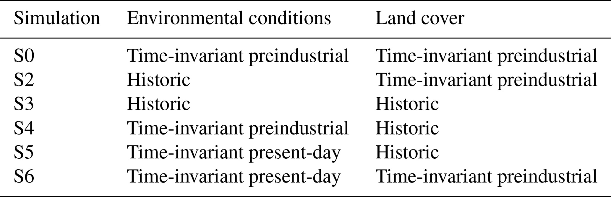
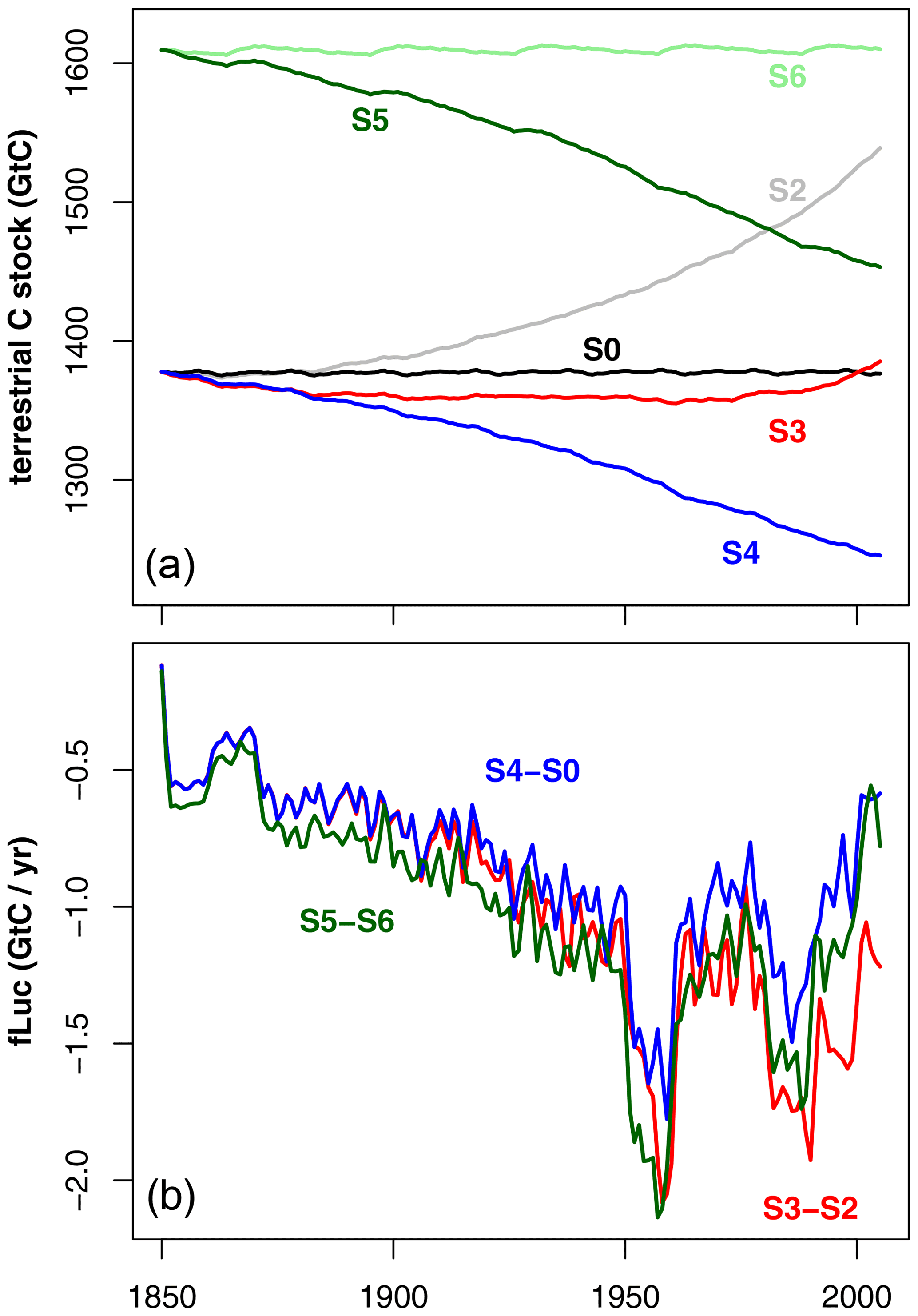
Figure 3 Terrestrial cumulative C stocks (a) and corresponding F_LUC (b) as simulated by the JSBACH dynamic vegetation model for the different simulations discussed. Shown is F_LUC derived as S5 minus S6, S3 minus S2, and S4 minus S0 (see text).​​​​​​​​​​​​​​

5.3 Remote-sensing data related to LUC

Several global remote-sensing products can be useful in estimating F_LUC in RECCAP2. They can be applied in various ways. The first is by estimating land cover change in the recent decades to produce regional transition maps at finer spatial scales and with better accuracy than is currently available. These maps can then be used to force BK or DGVMs. The second is by providing finer-resolution and globally consistent maps of vegetation C densities (for undisturbed locations) that can be used in BK models. The third is by directly estimating changes in biomass C stocks, for instance using optical data (Harris et al., 2012) vegetation optical depth (Fan et al., 2019), or lidar data, and report these values for deforestation areas only (to exclude environmentally induced fluxes).

Examples of already available remote-sensing-based datasets than can be used for land cover and land cover change mapping are the ESA-CCI land cover product, based on five different satellite missions at 300 m spatial resolution and annual time steps between 1992 and 2018 (ESA, 2017), and the Landsat 30 m spatial-resolution forest cover change product, covering 2000 to 2018 (Hansen et al., 2013) and extended to land cover change for forest, short vegetation, and bare soil (Song et al., 2018). For vegetation C densities, the ESA GlobBiomass dataset provides aboveground biomass data for a period centered on the year 2010 at 100 m spatial resolution (Santoro, 2018). Because of its fine spatial resolution, this dataset could, in principle, be used to evaluate undisturbed C densities (Erb et al., 2018; Luyssaert et al., 2012). Other datasets currently under development include the ESA-CCI high-resolution land-cover product, expected to provide a long-term record since the 1990s of regional high-resolution land cover maps at 30 m spatial resolution every 5 years in regions of interest, and the ESA-CCI biomass dataset, which will provide aboveground biomass data for four epochs, i.e., the mid-1990s, 2007–2010, 2017/2018, and 2018/2019, at 100 m spatial resolution with a relative error of less than 20 %. The NASA Carbon Monitoring System program is also supporting the development of regional- to global-scale biomass products based on optical reflectance data from MODIS (as well as active lidar-based approaches using ICESAT-1 and now ICESAT-2 GLAS-retrievals) and the Global Ecosystem Dynamics Instrument or GEDI aboard the International Space Station. The lidar approaches require integration with wall-to-wall optical measurements as lidar is a “shot” retrieval with a fairly small footprint size but has high accuracy in terms of measurement ability when retrieving canopy height and thus biomass (Dubayah et al., 2020). Satellite-based products have important advantages for estimating contemporary direct emissions from changes in aboveground biomass, such as global coverage, consistency, reliability, and increasingly higher spatial resolution. However, they cannot estimate legacy soil fluxes from land use change prior to the satellite era, and they are also unable to separate the contribution of environmental changes to F_LUC. The comparison of FLUC derived from RS-based methods with DGVMs or BK estimates should therefore be made with care.

5.4 National inventories

National Greenhouse Gas Inventories (NGHGIs) report anthropogenic emissions and sinks to the UNFCCC and are the official numbers used to take stock of the nationally determined contributions (NDCs). NGHGI use different definitions and assumptions than those used by the carbon cycle research community, as detailed in Grassi et al. (2018). NGHGI, in their agriculture forestry and land use (AFOLU) sector, report CO₂ fluxes of managed land, as defined by each country. Such managed land can include areas under nature conservation management. The C balance of established cropland, grassland, and forests are reported by national inventories under the LULUCF sub-sectors. The C fluxes of land use change transitions involving managed lands are reported separately based on national data on the area of different land use types. The carbon fluxes associated with transitions older than 20 years old are ignored. A variety of approaches are used by NGHGIs, mostly based on general emission factors following IPCC guidelines. Only lands converted within the past 20 years are included under LULUCF fluxes, unlike BK and DGVMs that calculate land use change fluxes since 1700 or 1850 CE. On the other hand, NGHGIs include land use change fluxes for transitions that are usually not implemented in BK and DGVMs, such as from peatland converted to agriculture and from land converted to human settlements.

5.5 Land use change transitions, definitions, and assumptions

The land use change transitions and land management fields used in the latest version of the GCP Global Carbon Budget (Friedlingstein et al., 2019) to calculate the net land use change flux, called F_{LUC latest}, are from the harmonized land use change data (LUH2v2.1h) dataset (Hurtt et al., 2011), which is based on HYDE3.1 (Klein Goldewijk et al., 2011). These data have the advantage of being globally consistent and covering a long period (850 CE–present) but have relatively coarse spatial resolution (0.25 × 0.25^∘), and due to a globally consistent methodology they may not account for regional specificities (Bastos et al., 2018; Li et al., 2018). For each region, the best available information (in terms of spatiotemporal resolution or detail of processes covered) on land use change should be used. This can be from national statistics, inventories, or remote sensing. In RECCAP2, each regional team will decide the land cover classification scheme that best fits a given region, but it is recommended that the LUH2v2h forest and non-forest distinction be used when classifying rangelands.

6 Concluding remarks

We present a way forward for developing consistent top-down and bottom-up estimates for regional carbon dioxide budgets. The methodology focuses on reconciling the treatment of non-CO₂ emissions from CH₄, CO, and BVOCs and their contribution to CO₂ via atmospheric chemistry and the treatment of lateral fluxes of carbon. Given the complexity of this task, the approaches toward implementation can be considered using the tiered approach of the IPCC, whereby higher tiers use progressively more complex regionally and locally calibrated sources of information. For example, a Tier 1 approach combines global emission factors with activity data to estimate fluxes, Tier 2 uses regionally calibrated emission factors, whereas Tier 3 uses locally calibrated emission factors to estimate fluxes from activity information. The Global Carbon Project now conducts greenhouse gas budget accounting for the three major greenhouse gases, i.e., carbon dioxide, methane, and nitrous oxide, where each budget provides detailed sectoral information for sources and sinks using a system that is more closely aligned with Tier 1 approaches. Beginning with Tier 1 data can help initiate regional budgets and identify areas of uncertainty or opportunities for regionally and locally calibrated approaches to be used to reduce uncertainty.