A zero-dimensional view of atmospheric degradation of levoglucosan (LEVCHEM_v1) using numerical chamber simulations

Here, we developed a zero-dimensional (0-D) modeling framework (LEVCHEM_v1) to provide insights into the atmospheric degradation of a key tracer emitted during biomass burning – levoglucosan (LEV), while additionally exploring its effects on the dynamics of secondary organic aerosols (SOA) and other gases. For this, we updated existing chemical mechanisms (homogeneous gas-phase chemistry and heterogeneous chemistry) in the BOXMOXv1.7 model to include the chemical degradation of LEV and its intermediary degradation products in both phases (gas and aerosol). In addition, we added a gas-particle partitioning mechanism to the model to account for the effect of evaporation and condensation on the phase-specific concentrations of LEV and its degradation products. Comparison of simulation results with measurements from various chamber experiments (spanning summer and winter conditions) show that the degradation timescale of LEV varied by phase, with gas-phase degradation occurring over ∼1.5–5 d and aerosol-phase degradation occurring over ∼8–36 h. These relatively short timescales suggest that most of the initial LEV concentration can be lost chemically or deposited locally before being transported regionally. We varied the heterogeneous reaction rate constant in a sensitivity analysis (for summer conditions only) and found that longer degradation timescales of LEV are possible, particularly in the aerosol phase (7 d), implying that some LEV may be transported regionally.

The multiphase chemical degradation of LEV has effects on SOA and other gases. Several first- or second-generation products resulted from its degradation; most of the products include one or two carbonyl groups, one product contains a nitrate group, and a few products show the cleavage of C−C bonds. The relative importance of the products varies depending on the phase and the timing of the maximum concentration achieved during the simulation. Our estimated secondary organic aerosol SOA yields (4 %–32 %) reveal that conversion of LEV to secondary products is significant and occurs rapidly in the studied scenarios. LEV degradation affected other gases by increasing the concentrations of radicals and decreasing those of reactive nitrogen species. Decreases of the mixing ratios of nitrogen oxides appear to drive a more rapid increase in ozone compared with changes in volatile organic compounds levels.

An important next step to confirm longer degradation timescales will be to extend the evaluation of the modeled LEV degradation beyond 3–6 h by using more extensive data from chambers and, possibly, from fire plumes. The mechanism developed here can be used in chemical transport models applied to fire plumes to trace LEV and its degradation products from source to deposition, to assess their atmospheric implications and to answer questions relevant to fire tracing, carbon and nitrogen cycling, and climate.

1 Introduction

Knowledge of the atmospheric lifetimes of biomass burning emissions is critical to predict their impacts on photochemistry, air quality and climate. The organic compounds in these emissions are denoted as pyrogenic carbon (PyC) and together they cover a wide range of chemistries and phases, making the determination of individual lifetimes challenging. In the atmosphere, PyC can be in the condensed phase (predominantly as semi- and non-volatile particulate matter, PM) and/or in the gas phase (volatiles). Both phases participate in atmospheric photochemistry. For instance, volatile organic compounds (VOCs) react with hydroxyl radical (OH) and contribute to tropospheric ozone (O₃) formation. Other gases released during biomass burning, such as polycyclic aromatic hydrocarbons, can be oxidized, the products of which may form semi- or non-volatile PM. Both directly emitted and secondarily formed PM alters visibility (through light extinction), human health (through respiration) and climate forcing (via absorption and/or scattering of solar radiation). Depending on its chemical and physical properties, PM also participates in cloud formation as cloud condensation nuclei and influences the physics and chemistry of clouds. Through alterations of physical properties of clouds, PM indirectly contributes to climate forcing. The magnitude and the extent of the impacts of PyC depend on its atmospheric lifetime.

Anhydrosugars, the most abundant of which is levoglucosan (LEV), are molecular tracers of PyC that have traditionally been used as markers for biomass burning in ambient aerosols, or as markers for wildfires in sediments and ice cores (Suciu et al., 2019, and references therein). However, their degradation and lifetimes are not well understood in any environment, including the atmosphere and cryosphere – two environments that are related via atmospheric transport and deposition of such PyC tracers. Therefore, understanding the atmospheric fate of anhydrosugars is essential not only to comprehending fire effects on air quality but also to interpreting fire records in ice and to studying the complex relationship between fire, vegetation and climate.

Experimental laboratory studies (in chambers or flow tubes) on LEV chemical degradation suggest that its atmospheric lifetimes vary widely, from minutes to months (Hennigan et al., 2010; Hoffman et al., 2010; Kessler et al., 2010; Knopf et al., 2011; Bai et al., 2013; Lai et al., 2014; Slade and Knopf, 2014; Arangio et al., 2015; Gensch et al., 2018; Pratap et al., 2019). In addition, the multiphase chemistry of LEV and its gas-particle partitioning (G $/$ P) between phases has not yet been explicitly considered in laboratory studies of its chemical kinetics. Given its semi-volatile nature, the evaporation and/or condensation effect in conjunction with chemical kinetics must be given attention in the estimation of LEV lifetimes, especially of those with respect to chemical degradation. Some models, such as the non-equilibrium kinetic evaporation model of May et al. (2013) consider this. Previous studies have applied the gas-particle partitioning model of May et al. (2013) to levoglucosan, but its multiphase chemical decay was limited to the reaction with the OH radical only (Pratap et al., 2018, 2019).

To more accurately estimate the atmospheric degradation timescales (modeled decay of concentration over time relative to initial concentration), anhydrosugar chemistry must be studied in more complex atmospheric settings than those reproduced in the laboratory. This could be achieved using three-dimensional (3-D) chemical transport models (CTMs). However, current CTMs do not treat anhydrosugars individually in their chemical mechanisms. This is partly because these models are often motivated by the need to quantify only PM mass in order to meet air quality legislation. Thus, studies often report modeled species such as PM_2.5 (PM with diameters smaller than 2.5 µm), organic carbon in PM (OC), and black carbon (BC) (In et al., 2007; Alvarado et al., 2009, 2015; Simon and Bhave, 2012; Pye and Pouliot, 2012; Heron-Thorpe et al., 2014). Moreover, because anhydrosugars are also semi-volatile, they participate in both gas- and aerosol-phase chemistries, so placing them into just one single category (i.e., PM_2.5) is inaccurate. In general, individual emissions from biomass burning are lumped into categories, assuming that all species behave identically with respect to chemical and physical transformation or loss. While this assumption eases the computational burden of the chemistry and physics of the model, it can yield inaccurate results regarding the modeled species; it also does not allow the study of tracers individually.

Here, we developed a zero-dimensional (0-D) modeling framework (LEVCHEM_v1) to study the chemical degradation of LEV. Because the two isomers of LEV (mannosan and galactosan) have similar structures but different arrangements of the hydroxyl groups, this study only focuses on chemical reactions involving LEV. A future goal is to expand LEVCHEM_v1 to include the degradation of the two isomers and, then, to implement the full mechanism of anhydrosugar degradation into 3-D CTMs. The 0-D modeling approach here can identify model uncertainty attributable to the mechanism only; when the mechanism is used in a CTM, other sources of uncertainty (advection, diffusion, deposition, etc.) in the overall uncertainty of the model predictions can be assessed.

Several research topics pertinent to the chemical degradation of LEV are dealt with in this study. These will be addressed after a discussion of the model framework and development.

First, we explore the degradation timescale of LEV, and what can be inferred from it regarding the scale of its impact (local vs. regional). For example, isolating the effect of chemistry from transport or other physical processes may yield different degradation timescales, resulting in different inferred transport distances, impacting whether local- or regional-scale chemistry may be the dominant process controlling the lifetime of LEV.

Second, we examine the contribution of LEV degradation to the formation of secondary organic aerosols (SOA), including changes in total PM mass and the relative importance of degradation products. Significant LEV degradation may lead to higher SOA yields. This information can further be used as a reference to understand SOA formation in a 3-D CTM framework.

Third, we examine how LEV degradation affects the concentrations of other gases such as O₃ and its precursors, nitrogen oxides (NO_x = nitric oxide (NO) + nitrogen dioxide (NO₂)) and VOCs, total reactive nitrogen (NO_y) and NO_x oxidation products (NO${}_z={\mathrm{NO}}_y-{\mathrm{NO}}_x$). Considering its multiphase chemistry that also generates peroxy radicals (RO₂), LEV may have an important effect on these pollutants.

2 Modeling approach

2.1 Overview of the 0-D modeling framework and mechanisms

The 0-D model used to develop LEVCHEM_v1 in this study (BOXMOX v1.7) (Knote et al., 2015) is a publicly available software that expands on earlier code, the Kinetic PreProcessor (KPP v2.1) (Sandu and Sander, 2006). The two models are briefly described below.

The KPP generates code using chemical reactions and their respective reaction rate coefficients as inputs (Sandu and Sander, 2006). The rate of change in the concentration of a species i ($\frac{\mathrm{d}{C}_i}{\mathrm{d}t}$) is expressed as the difference between its production (P) and loss (L) rates (Eq. 1).

$$\begin{array}{}\text{(1)}& {\displaystyle \frac{\mathrm{d}{C}_i}{\mathrm{d}t}}=P-L\end{array}$$

The generated code (which determines the P and L terms in Eq. 1) is then used in a temporal integration to compute the change in concentration of the individual reactants and products based on a system of ordinary differential equations (ODE).

The KPP offers a variety of stiff numerical integrators that can be selected by the user in order to maximize the computational efficiency of the ODE system within a low to medium accuracy regime (Sandu and Sander, 2006).

The BOXMOX extends the KPP capabilities even further by providing a framework in which various numerical experiments are possible, such as chamber experiments or boundary layer atmospheric chemistry numerical experiments (Knote et al., 2015). These are possible with the addition of a wrapper to the KPP. The wrapper allows the user to add inputs to the model, such as initial conditions, environmental conditions, boundary conditions, time-varying photolysis rates, turbulent mixing, emissions and deposition, in order to run numerical experiments; it also allows the user to add new code to further develop the model. The model outputs time series of species concentrations, rate constants and other user-specified information.

2.2 Mechanistic development

We integrated the multiphase chemical degradation of LEV into BOXMOXv1.7 by adding chemical reactions along with their reaction rate coefficients to existing homogeneous gas-phase and heterogenous mechanisms (LEVCHEM_v1). These existing mechanisms already have been implemented and tested by the BOXMOXv1.7 developers (Knote et al., 2015).

Based on its similarity to mechanisms used in 3-D CTMs, we chose the Carbon Bond version 2005 with toluene updated chlorine chemistry as the homogeneous gas-phase mechanism to implement the gas-phase degradation of LEV. This was recently updated by the United States Environmental Protection Agency to include additional tropospheric chemistry (CB05TUCl_EPA). It contains 148 chemical reactions that constitute the core of the mechanism or the “CB05” part (Yarwood et al., 2005; Whitten et al., 2010), 23 reactions for the reactive chlorine chemistry or the “TUCl” part, 10 reactions for formation of secondary aerosols from gas–gas reactions, and 24 photolysis reactions (Knote et al., 2015). In total, the overall gas-phase mechanism included 205 reactions and 82 variable species to describe gas-phase tropospheric photochemistry. Here, we extended the CB05TUCl_EPA mechanism to include 13 reactions and 10 species (radicals and first- or second-generation products) associated with LEV chemistry in the gas phase (see Table 1). (Chemical structures are shown in Figs. S1 and S2 in the Supplement.) Thus, the total number of reactions and species in the updated gas-phase mechanism increased to 218 and 99, respectively.

Table 1 Homogeneous gas-phase mechanism.

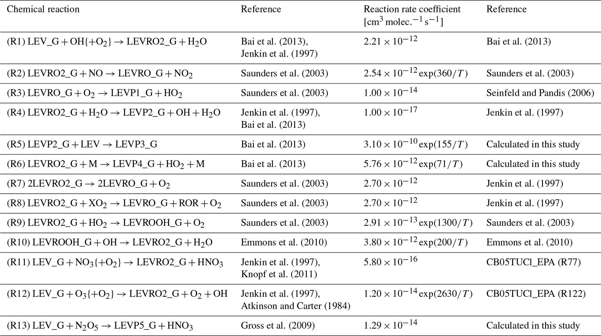
{ } Species concentration not included in the reaction rate (i.e., reaction of LEV_G radical with O₂ is assumed to be instantaneous).

The homogeneous gas-phase reaction rate coefficients (Table 1) were modeled as constants (when available in the literature) or as Arrhenius-type reaction rate coefficients (Eq. 2) using functions developed previously (Knote et al., 2015) with measured, assumed or calculated parameters:

$$\begin{array}{}\text{(2)}& k=A\times \exp \left({\displaystyle \frac{-E}{RT}}\right),\end{array}$$

where k is the homogeneous second-order gas-phase reaction rate coefficient (${\mathrm{cm}}^{\mathrm{3}}\mathrm{molec}{.}^{-\mathrm{1}}{\mathrm{s}}^{-\mathrm{1}}$), A is the collision frequency factor (${\mathrm{cm}}^{\mathrm{3}}\mathrm{molec}{.}^{-\mathrm{1}}{\mathrm{s}}^{-\mathrm{1}}$), E is the energy barrier for the reaction (kJ mol⁻¹), R is the ideal gas law constant (8.314 $\mathrm{J}{\mathrm{mol}}^{-\mathrm{1}}{\mathrm{K}}^{-\mathrm{1}}$) and T is temperature (K).

When the collision rate coefficient A was not available in the literature, we calculated it using Eq. (3) (Seinfeld and Pandis, 2006) applied to two spherical bodies (molecules) A and B:

$$\begin{array}{}\text{(3)}& A=\mathit{\pi }{d}^{\mathrm{2}}\sqrt{\left({\displaystyle \frac{\mathrm{8}{k}_{\mathrm{B}}T}{\mathit{\pi }\mathit{\mu }}}\right)}\end{array}$$

Here, d² represents the squared sum of the two radii of A and B (m²), and the term under the square root is the relative velocity of the A and B collision bodies in which k_B is the Boltzmann constant ($\mathrm{1.381}\times {\mathrm{10}}^{-\mathrm{23}}$ J K⁻¹) and μ is the reduced mass (Eq. 4):

$$\begin{array}{}\text{(4)}& \mathit{\mu }={\displaystyle \frac{m_{\mathrm{A}}\times m_{\mathrm{B}}}{\left(m_{\mathrm{A}}+m_{\mathrm{B}}\right)}}\end{array}$$

The heterogeneous chemical mechanism HETCHEM was developed by Knote et al. (2015) to model the heterogeneous interaction between dinitrogen pentoxide (N₂O₅) and water bound to solid aerosols or PM. The heterogeneous reaction rate (k_{SFC_REACTION}) was modeled by Knote et al. (2015) based on first-order surface uptake from Fuchs and Sutugin (1971) (Eq. 5):

$$\begin{array}{}\text{(5)}& k_{\text{SFC\_REACTION}}={\displaystyle \frac{\mathrm{1}}{\mathrm{4}}}\times \mathit{\gamma }\times \mathit{\omega }\times \text{SAD},\end{array}$$

where γ represents the uptake coefficient of the gas-phase oxidant species i (ranging from 0 to 1), ω is the mean molecular velocity (m s⁻¹) and SAD is the aerosol surface area density (m² m⁻³). The mean molecular velocity is calculated via Eq. (6):

$$\begin{array}{}\text{(6)}& \mathit{\omega }=\mathrm{1.455}\times {\mathrm{10}}^{\mathrm{2}}\times \sqrt{{\displaystyle \frac{T}{\text{MW}\times {\mathrm{10}}^{\mathrm{3}}}}},\end{array}$$

where T is the temperature (K), and MW is the molecular weight of the gas species (kg mol⁻¹).

Table 2 Heterogeneous mechanism.

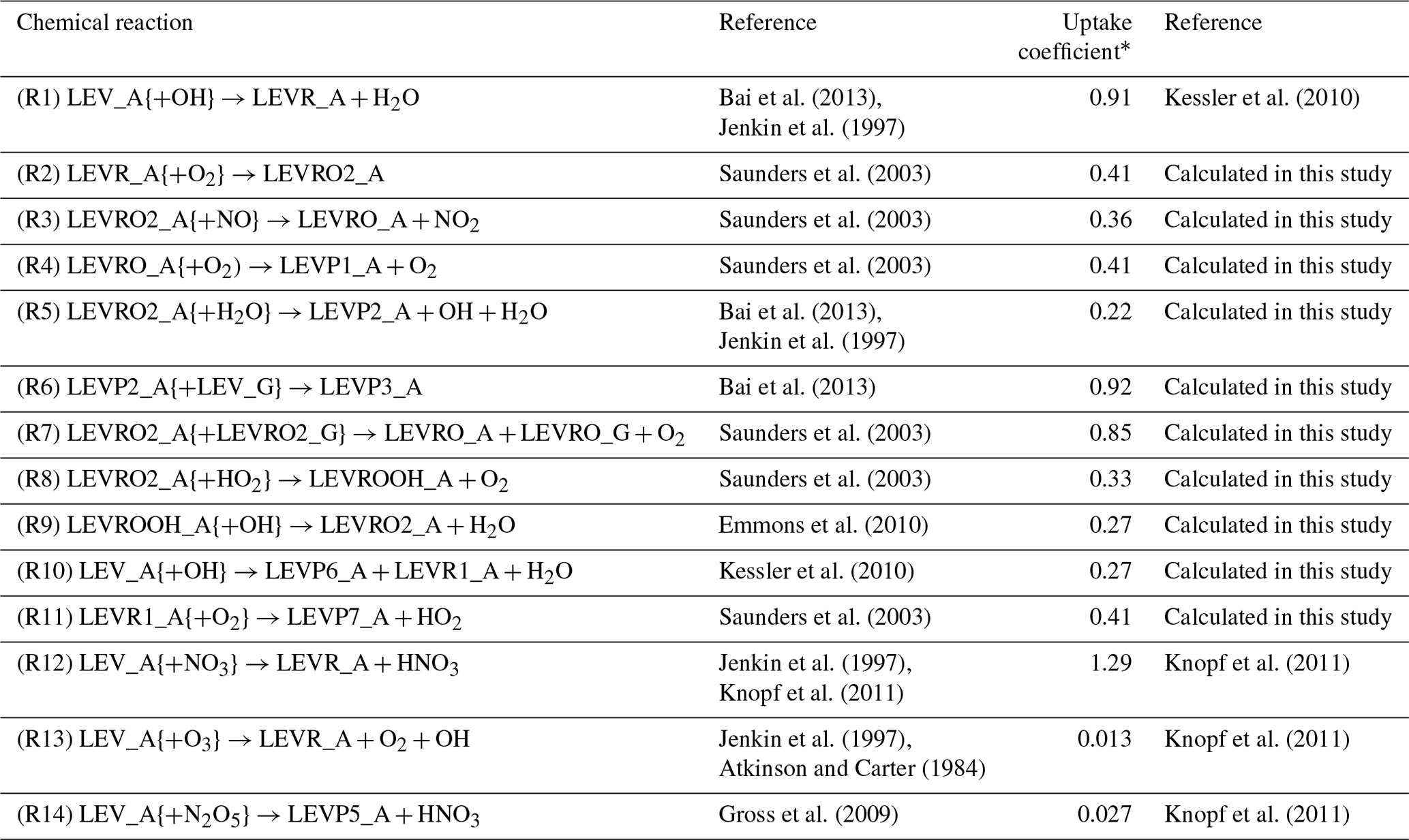
^* The uptake coefficient used in the calculation of the heterogeneous reaction rate coefficient (see Eq. 5).

Using the same expression for the heterogeneous reaction rate as in Eq. (5), we implemented the heterogeneous chemistry of LEV in the form of first-order reactions (see Table 2) and using uptake coefficients (γ) available from literature (experimental measurements) or calculated in this study based on the collision theory (Seinfeld and Pandis, 2006), thermodynamic parameters from Bai et al. (2013), and the relationship between γ and the second-order heterogeneous reaction rate constant for the reaction of LEV with the OH radical (Kessler et al., 2010). When the uptake coefficient was not available in the literature, Eq. (7) was used to calculate the uptake coefficient for the heterogeneous reaction of particle-phase LEV (and its degradation products):

$$\begin{array}{}\text{(7)}& {\mathit{\gamma }}_{i,\mathrm{OH}}={\displaystyle \frac{\mathrm{2}{D}_{\mathrm{0}}{\mathit{\rho }}_i{N}_{\mathrm{A}}}{\mathrm{3}{\overline{c}}_{\text{OH}}{M}_i}}{k}_{i,\mathrm{OH}},\end{array}$$

where γ_i,OH is the effective gas-phase oxidant uptake coefficient by species i (here, the gas-phase oxidant is OH), D₀ is the surface-weighted average diameter of the particle at the beginning of the experiment (in this study, the particle diameter was assumed to be constant throughout the simulations and is denoted as D_p), ρ_i is the density of the organic species, N_A is Avogadro's number (6.022×10²³ $\mathrm{molec}.{\mathrm{mol}}^{-\mathrm{1}}$), ${\overline{c}}_{\text{OH}}$ represents the average velocity of the gas-phase OH radical (or other oxidant), M_i is the molecular weight of the organic species and k_i,OH is the second-order heterogeneous reaction rate constant. This study used an average of several heterogeneous reaction rate constants ($\mathrm{2.85}\times {\mathrm{10}}^{-\mathrm{13}}$ ${\mathrm{cm}}^{\mathrm{3}}\mathrm{molec}{.}^{-\mathrm{1}}{\mathrm{s}}^{-\mathrm{1}}$) measured by Slade and Knopf (2014). We assumed this value for all LEV degradation products (including for the radical LEVROOH; see Reaction R9 in Table 2) due to the fact that experimental heterogeneous reaction rate coefficients have not been measured for LEV products.

The G $/$ P mechanism used in this study (as part of LEVCHEM_v1) was taken from May et al. (2013) and describes the rate of change in concentration of both gas-phase and particle-phase species due to evaporation and condensation (Eqs. 8, 9).

$$\begin{array}{}\text{(8)}& {\displaystyle \frac{\mathrm{d}{C}_{\mathrm{p},i}}{\mathrm{d}t}}=-\text{CS}\left(X_{\mathrm{m},i}{\text{Ke}}_i{C}_i^{\ast }-C_{\mathrm{g},i}\right)\text{(9)}& {\displaystyle \frac{\mathrm{d}{C}_{\mathrm{g},i}}{\mathrm{d}t}}=-{\displaystyle \frac{\mathrm{d}{C}_{\mathrm{p},i}}{\mathrm{d}t}}\end{array}$$

Changes in the particle-phase concentration (C_p,i) are tracked simultaneously based on the difference between the gas-phase concentration of species i(C_g,i) and the theoretical surface equilibrium concentration ($C_i^{\ast }$) (Eq. 10), corrected for the mass fraction of species i in the particle phase (X_m,i) (Eq. 11) and the Kelvin effect (Ke_i) (Eq. 12):

$$\begin{array}{}\text{(10)}& C_i^{\ast }\left(T\right)=C_i^{\ast }\left(\mathrm{298}\mathrm{K}\right)\exp \left[-{\displaystyle \frac{\mathrm{\Delta }{H}_{\text{vap},i}}{R}}\left({\displaystyle \frac{\mathrm{1}}{T}}-{\displaystyle \frac{\mathrm{1}}{\mathrm{298}\mathrm{K}}}\right)\right]{\displaystyle \frac{\mathrm{298}\mathrm{K}}{T}},\end{array}$$

where $C_i^{\ast }\left(\mathrm{298}\mathrm{K}\right)$ represents the saturation concentration of species i at 298 K, and ΔH_vap,i is the enthalpy of vaporization of species i. From a mass balance, the changes in the two concentrations are equal but opposite in sign.

$$\begin{array}{}\text{(11)}& X_{\mathrm{m},i}={\displaystyle \frac{f_i{C}_{\text{tot}}}{C_{\text{OA}}}}{\left(\mathrm{1}+{\displaystyle \frac{C_i^{\ast }\left(T\right)}{C_{\text{OA}}}}\right)}^{-\mathrm{1}},\end{array}$$

where f_i represents the mass fraction of the organic species i, C_tot is the total concentration of the organics (gas and aerosol phases) and C_OA is the total concentration of organic aerosols.

$$\begin{array}{}\text{(12)}& \text{Ke}={\displaystyle \frac{\mathrm{4}\mathit{\sigma }{\text{MW}}_i}{\mathit{\rho }RT{D}_{\mathrm{p}}}},\end{array}$$

where σ represents the surface tension of the bulk particle, MW_i is the molecular weight of the organic species i, ρ is the bulk density of the particle and D_p is the particle diameter.

The first-order condensation sink (CS) (Eq. 13) is a function of D_p, total particle number concentration (N_t), the diffusion coefficient of the organic vapor in air (D) and the Fuchs–Sutugin correction factor (C_F-S) that accounts for effects of non-continuity (Eq. 14).

$$\begin{array}{}\text{(13)}& \text{CS}=\mathrm{2}\mathit{\pi }{D}_{\mathrm{p}}{N}_{\mathrm{t}}D{C}_{F\text{-}S}\end{array}$$

The C_F-S depends on the Knudsen number (Kn) and the mass accommodation coefficient (α).

$$\begin{array}{}\text{(14)}& C_{F\text{-}S}={\displaystyle \frac{\mathrm{1}+\mathit{Kn}}{\mathrm{1}+\mathrm{0.3773}\mathit{Kn}+\mathrm{1.33}\mathit{Kn}\frac{\mathrm{1}+\mathit{Kn}}{\mathit{\alpha }}}}\end{array}$$

The dimensionless Knudsen number (Eq. 15) is defined as the ratio between the mean free path of air (λ=62.5 nm) and the particle radius ($D_{\mathrm{p}}/\mathrm{2})$.

$$\begin{array}{}\text{(15)}& \mathit{Kn}=\mathrm{2}{\displaystyle \frac{\mathit{\lambda }}{D_{\mathrm{p}}}}\end{array}$$

The mass accommodation coefficient represents the probability of a vapor sticking to the particle surface once a collision occurs; numerically, α ranges from zero (no accommodation) to one (perfect accommodation) (Seinfeld and Pandis, 2006).

2.3 Simulations and sensitivity analysis

For both model evaluation and sensitivity, we ran multiple 7 d simulations at a 10 s temporal resolution in various scenarios, from fast (the default case) to relatively slower heterogeneous chemistry. The heterogeneous chemistry was varied to account for other controls on LEV concentration that were not explicitly considered in the present 0-D modeling approach, such as aerosol matrix effects (composition, mixing state, multilayer kinetics, liquid water content, etc.). These additional controls were lumped into a single factor (F) which, for model evaluation, was assumed to vary according to the conditions in chamber experiments. We expect F to be, at a maximum, 0.1 due to observed mass fractions in biomass burning organic aerosols (Sullivan et al., 2014). However, for sensitivity analysis, we varied F from 1.0 (default case) to lower values (0.1, 0.01 and 0.001) to slow down the heterogeneous reaction rates. In addition, we varied the mass accommodation coefficient (see Eq. 14) from a default case of 0.1 (which is the lower limit of α for a system in equilibrium; May et al., 2013) to lower values (0.01 and 0.001) and larger values (1.0). It was necessary to vary α because its value is unknown for levoglucosan and its degradation products. The mass accommodation coefficient is related to the G $/$ P partitioning mechanism (Eq. 14) and the uptake coefficient (γ). Theoretically, α≥γ, depending on the Knudsen number (Kulmala and Wagner, 2001).

The initial conditions of aerosol-phase LEV represent the average of initial concentrations used in chamber experiments (Table S1 in the Supplement; Hennigan et al., 2010; Lai et al., 2014; Pratap et al., 2019). The initial LEV concentration in the gas phase was set to its vapor pressure in all the scenarios (Table S1). We estimated the initial conditions of other species in the chemical mechanism as well as photolysis rate constants by running 1 h resolution, daily 3-D CTM simulations (Community Multi-scale Air Quality Model, CMAQv5.0.2) using inputs (emissions and meteorology) from Rasool et al. (2016). These conditions correspond to the location, altitude and timing of a small prescribed-fire plume in South Carolina (Sullivan et al., 2014).

For aerosol property (D_p), air temperature, pressure and relative humidity values, we used values from chamber experiments (Table S1; Hennigan et al., 2010; Lai et al., 2014; Pratap et al., 2019). Other parameters (N_t, SAD, ΔH_vap,i, σ, $C_i^{\ast }\left(\mathrm{298}\mathrm{K}\right)$ and ρ) that were not measured in chamber experiments but were used in simulations are also given in Table S1.

3 Results and discussion

3.1 Model evaluation

We evaluated the model (LEVCHEM_v1) by comparing simulation outputs (i.e., concentration) with experimental chamber data in scenarios in which simulations were initialized using chamber conditions. In particular, we investigated the contributions of LEV degradation to SOA, the change in total PM mass and the effects on other gases like O₃ and NO_x. We also examined the sensitivity of the degradation timescale of LEV and SOA yields to model parameters.

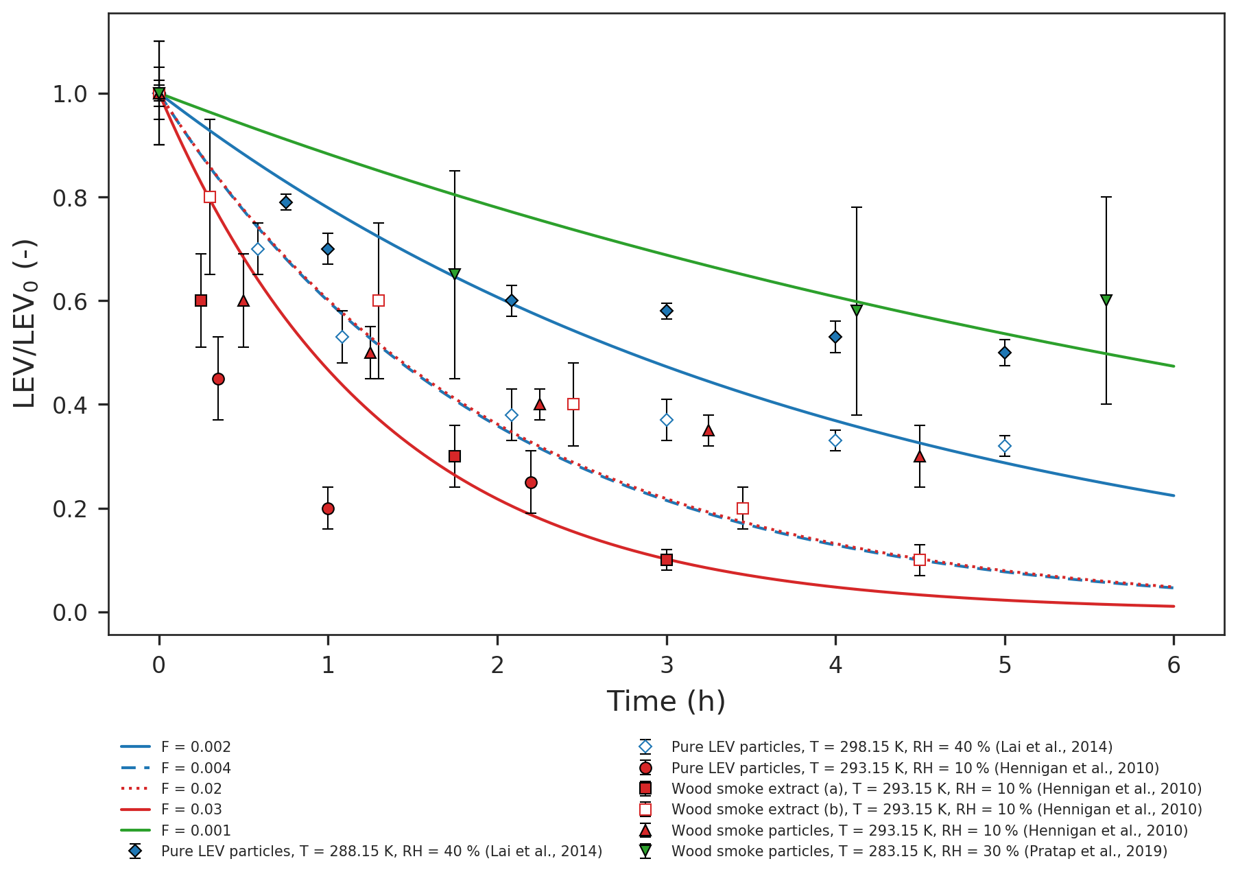
Figure 1 Simulated LEV degradation (lines) and measured LEV degradation (points); colors represent conditions from different chamber experiments taken from three studies (red – Hennigan et al., 2010; blue – Lai et al., 2014; green – Pratap et al., 2019) used in the simulations. LEV concentration is normalized by the initial concentration (LEV/LEV₀).

We evaluated the two-phase (gas–aerosol) modeling of LEV degradation by comparing the time series of the aerosol LEV concentration resulting from simulations to those obtained from laboratory chamber experiments (only the particle-phase data) over 5–6 h (Fig. 1). Overall, the model predicted that LEV degradation closely follows the measured LEV degradation in relatively slower heterogeneous chemistry scenarios (F=0.001; 0.002; 0.004; 0.02; 0.03; depending on the experimental data considered) and at mass accommodation coefficients of 0.1 and 0.01. These α values are smaller than those of γ for most of the chemical species, including for levoglucosan. However, as seen in Table 2, the great majority of the γ values were computed in this study (in the absence of their experimental measurements). In Eq. (7), we assume a similar second-order heterogeneous reaction rate for all of the species; this may bias our calculations of γ towards larger values. For γ values on the order of 10⁻¹ (OH uptake by levoglucosan, for example) and Knudsen numbers on the order of 10⁻¹ (all modeled cases), the corresponding α should be ∼0.1, according to Fig. 1 in Kulmala and Wagner (2001). This is true when we model conditions from Hennigan et al. (2010); thus, in this case the α≥γ criterion is marginally satisfied. Modeled conditions from Lai et al. (2014) and Pratap et al. (2019) do not meet this criterion for levoglucosan because, for similar Kn and γ values, the model only worked well (compared to experimental data) at α=0.01; in these cases, α<γ. However, for other species with smaller γ (O₃ and N₂O₅), all of the modeled cases in our study satisfy the criterion α≥γ. It is worth noting here that the effective α values we found in our study by comparing model predictions with data have inherent uncertainties associated with both the data and the model. The 1 order of magnitude difference between F values may be explained by the different initial LEV concentration used in both experiments and simulations (which is 1 order of magnitude as well) and, to a smaller extent, by the differences in relative humidity (Table S1). For instance, Hennigan et al. (2010) used drier conditions in chamber experiments compared with Lai et al. (2014) and Pratap et al. (2019). However, the model does not capture fast degradation in one case (red dots) in the first hour of simulation or the plateau observed after 3 h (diamonds and triangles). While the first case may be explained by the uncertainty in the modeled heterogeneous reaction rate that is varied by F, the second case could be explained by the fact that, in chamber experiments, the buildup of matter at the surface of the aerosol prevents LEV in the aerosol from reacting with gases or partitioning to the gas phase. The scattering in the chamber data relative to model lines could also be explained by the different source of LEV used in chamber experiments compared with the model (wood smoke particles and smoke extract vs. pure LEV particles).

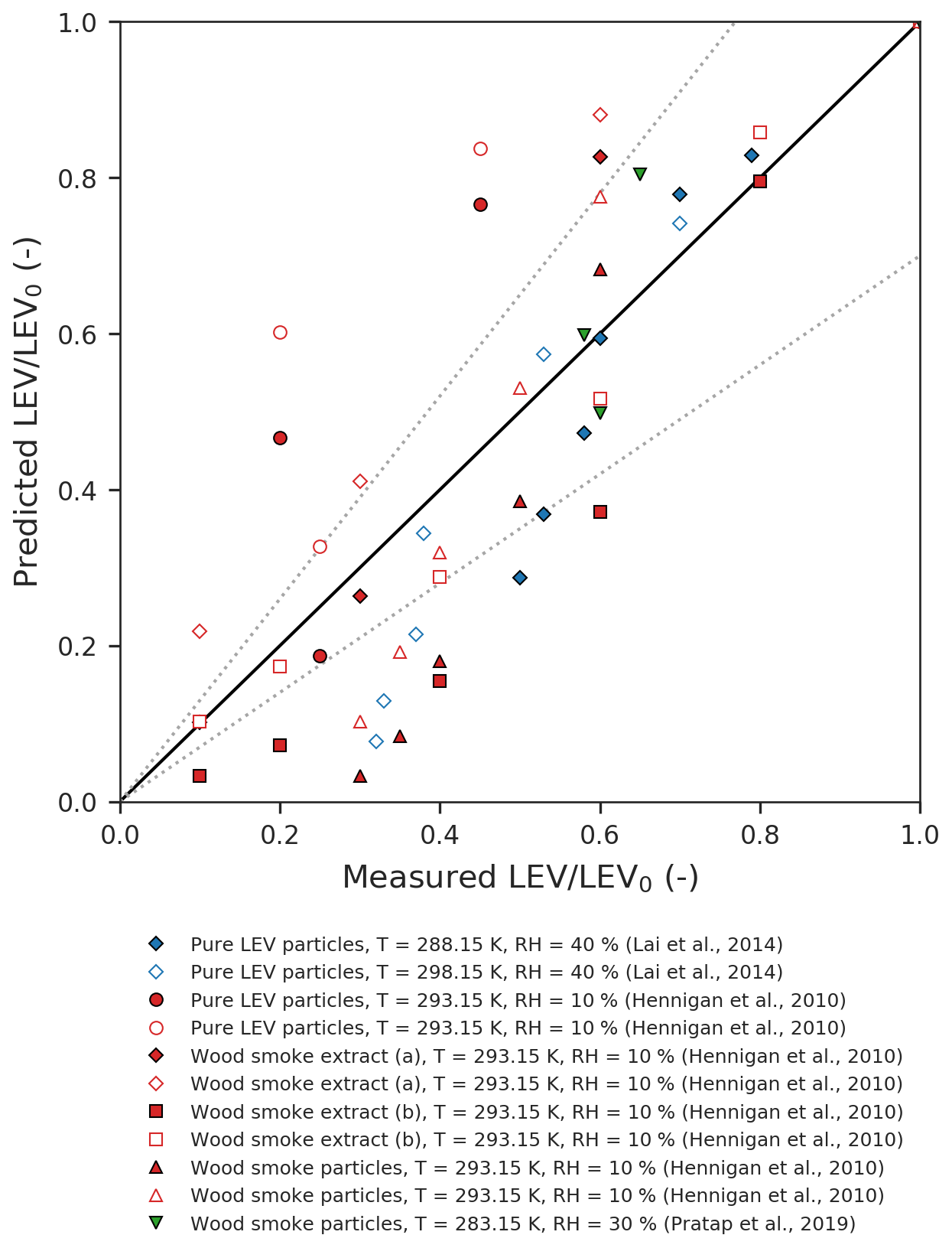
Figure 2 Parity plot of the predicted vs. measured LEV concentration (normalized by the initial concentration). The dotted lines represent the ±30 % error margins.

One-to-one comparison of predicted vs. measured LEV degradation (Fig. 2) from all of the simulated scenarios (red, blue and green) shows that the model performs very well for some of the data points (those that fall within the ±30 % limits) but the average absolute error of the model is relatively large (47 %). Overall, the model underpredicts the LEV concentration (average relative error of −47 %). The linear agreement between the model predictions and the experimental data is strong (coefficient of determination of 0.78).

While only the first 5–6 h of the simulations could be evaluated using chamber measurements, the simulated LEV degradation continued after this length of time until the LEV concentration was nearly zero, for 1.5–5 d in the gas phase and 8–36 h in the aerosol phase (Fig. 3). These longer timescales are a first estimate of degradation timescales of LEV.

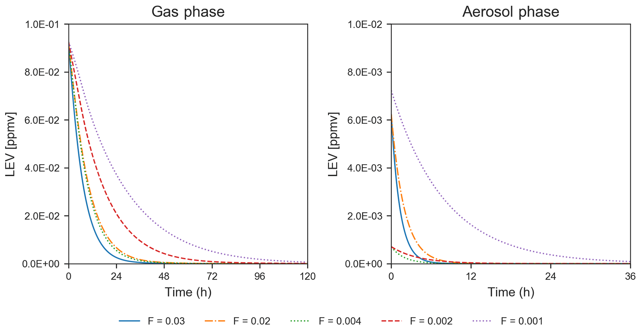
Figure 3 Degradation of LEV (conditions from Hennigan et al., 2010, when F=0.02–0.03 and α=0.1; from Lai et al., 2014, when F=0.002–0.004 and α=0.01; and from Pratap et al., 2019, when F=0.003 and α=0.01). Note the change in the scale of the axes between the two panels.

The relative importance of degradation products differs in the two phases (see Tables 1 and 2 for processes leading to formation of these products; also see Figs. S1 and S2 for chemical structures), with LEVP4 and LEVP5 dominating the gas phase and LEVP6, LEVP7 and LEVP2 dominating the aerosol phase over the first 5–6 h (Figs. S3, S4, S5, S6, S7 in Supplement). LEVP4 is a product formed only by the gas-phase chemistry (Reaction R6 in Table 1) and contains a carbonyl group after this reaction (Fig. S1). LEVP5 is a nitrated organic (Fig. S1) that is theoretically generated by both chemical mechanisms (Reaction R13 in Table 1 and Reaction R14 in Table 2). Products LEVP6 and LEVP7 (Fig. S1) are results of the fragmentation pathway specific only to heterogeneous chemistry (Reactions R10–R11 in Table 2); they both contain a carbonyl group (Fig. S1). LEVP2 is a product of Reaction (R4) (Table 1) and Reaction (R5) (Table 2); it contains two additional functional groups compared with LEV: a carbonyl and an ether (Fig. S1). The relative importance of products slightly changes beyond 5–6 h, particularly in the aerosol phase, in which LEVP3 becomes more important than LEVP2. LEVP3 is the largest molecular product (Fig. S1) that is generated by the multiphase LEV chemistry in Reactions (R5) (Table 1) and (R6) (Table 2). Through subsequent reactions, LEVP3 can grow into a larger molecule that would ultimately contribute to the nucleation of new PM (Bai et al., 2013).

3.2 Contribution of levoglucosan degradation to SOA

Traditionally, reactant organic species in the gas phase are considered to contribute to new SOA formation (or new SOA mass). However, in this study, as LEV is present in both phases and its chemistry generates products in both phases that can partition from one phase to another, both LEV_G (gas) and LEV_A (aerosol) can be treated as SOA precursors. Thus, they are both included in SOA yield calculation. Using Eq. (16), the SOA yield is calculated as the ratio between the mass of SOA formed and the mass of the reacted precursors (Stefenelli et al., 2019).

$$\begin{array}{}\text{(16)}& \begin{array}{rl}& \text{SOA yield}\left(\mathit{\%}\right)\\ & ={\displaystyle \frac{\sum _{i=\mathrm{1}}^n\text{LEVPi\_A}}{({\text{LEV\_G}}_{\mathrm{0}}+{\text{LEV\_A}}_{\mathrm{0}})-(\text{LEV\_G}+\text{LEV\_A})}},\end{array}\end{array}$$

where LEVPi_A represents a LEV oxidation product in the aerosol phase, subscript “0” refers to initial conditions and n=7. The terms represent mass concentrations. Formation of SOA from LEV degradation occurs rapidly (in the first 2–34 min of the simulation), with maximum SOA yields ranging from 4 % to 32 % (Fig. 4a). These high SOA yields in the first 6 h are the result of the rapid conversion of the precursors to aerosol-phase products, mainly due to heterogeneous chemistry. Because these products are not seen in the gas phase, evaporation does not influence the SOA yields in this early stage of the simulation; condensation of gas-phase products (LEVP4 and LEVP5) is also negligible (see Fig. S3–S7). Most of the oxidation products remain in the aerosol phase over the entire simulation period, except for LEVP5 and LEVP1 that may partition to the gas phase. SOA yield reaches steady state at ∼24–26 h due to near-zero concentrations of the two precursors and the presence of oxidation products from heterogeneous chemistry and G $/$ P partitioning (i.e., condensation of LEVP4) in the aerosol phase. Among the simulated scenarios, the largest SOA yields resulted when higher initial LEV_A concentrations were used in the simulations and they did not decrease below 8 % in wintertime conditions (Fig. 4 and Table S1). The heterogeneous chemistry was the slowest for SOA yields predicted for winter conditions (suggested by F=0.001), and it was the fastest for those associated with summer conditions (F=0.02–0.03). The total aerosol mass (the sum of concentrations of all LEV-related aerosol species, including the radicals) also increased by 8 %–15 % in the first 6 h and kept increasing, although at a slower pace, to up to 18 %–29 % at the end of the simulation period. The smallest total aerosol mass in the first 6 h (8 %) was observed in modeled wintertime conditions, whereas the highest total aerosol mass (14 %–15 %) was observed in summertime conditions. These suggest that the multiphase chemistry of LEV along with its phase partitioning cannot be ignored in assessments of fire air quality effects and can have variable effects on SOA yields depending on the initial conditions and aerosol properties.

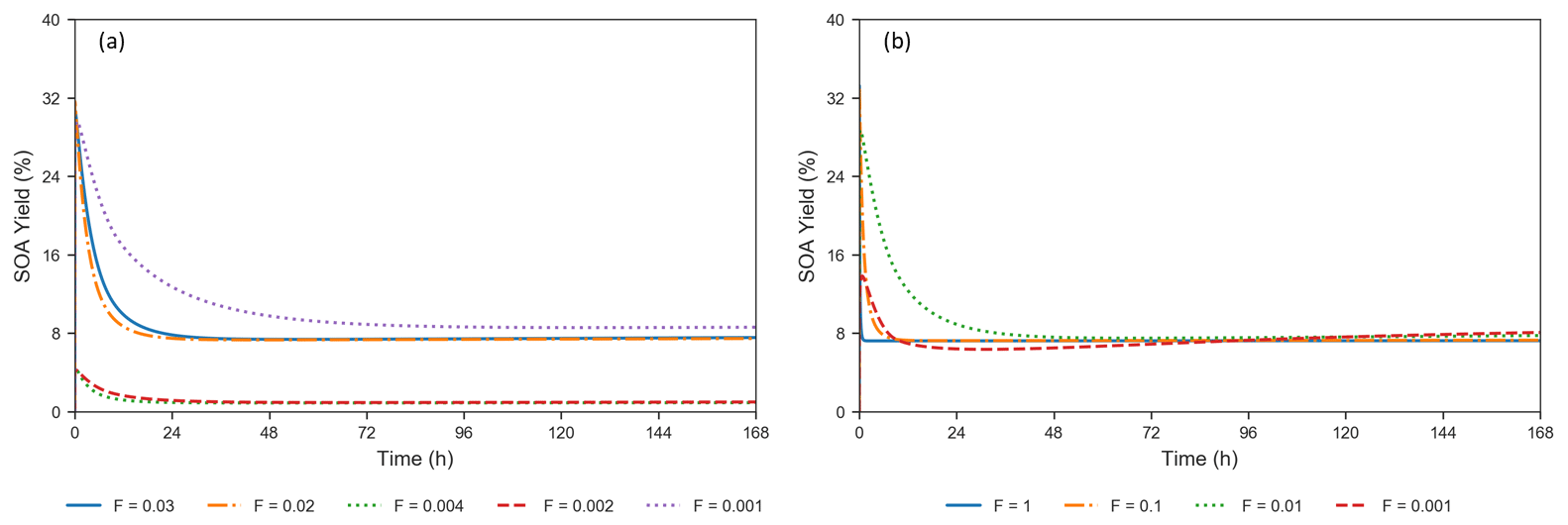
Figure 4 (a) Evolution of SOA yields from LEV degradation using valid simulations (conditions from Hennigan et al., 2010, when F=0.02–0.03 and α=0.1; from Lai et al., 2014, when F=0.002–0.004 and α=0.01; and from Pratap et al., 2019, when F=0.001 and α=0.01). (b) Effect of varying the heterogeneous reaction rate coefficient by 4 orders of magnitude, at a constant mass accommodation coefficient (α=0.1) (conditions from Hennigan et al., 2010).

3.3 Effects of LEV degradation on other gases

Implementation of LEV chemistry in models can also be used to consider its effects on other atmospheric species to better understand the effects of fire on air quality and atmospheric chemistry, such as the formation of tropospheric O₃ in the presence of NO_x and VOCs (both emitted from fires), conversion of NO_x to other reactive nitrogen forms (including nitrated LEV) and interaction with key gas-phase species oxidants. We studied effects in the model scenarios by comparing the concentrations of those key species obtained with LEV chemistry and those obtained without LEV chemistry (Figs. 5, 6).

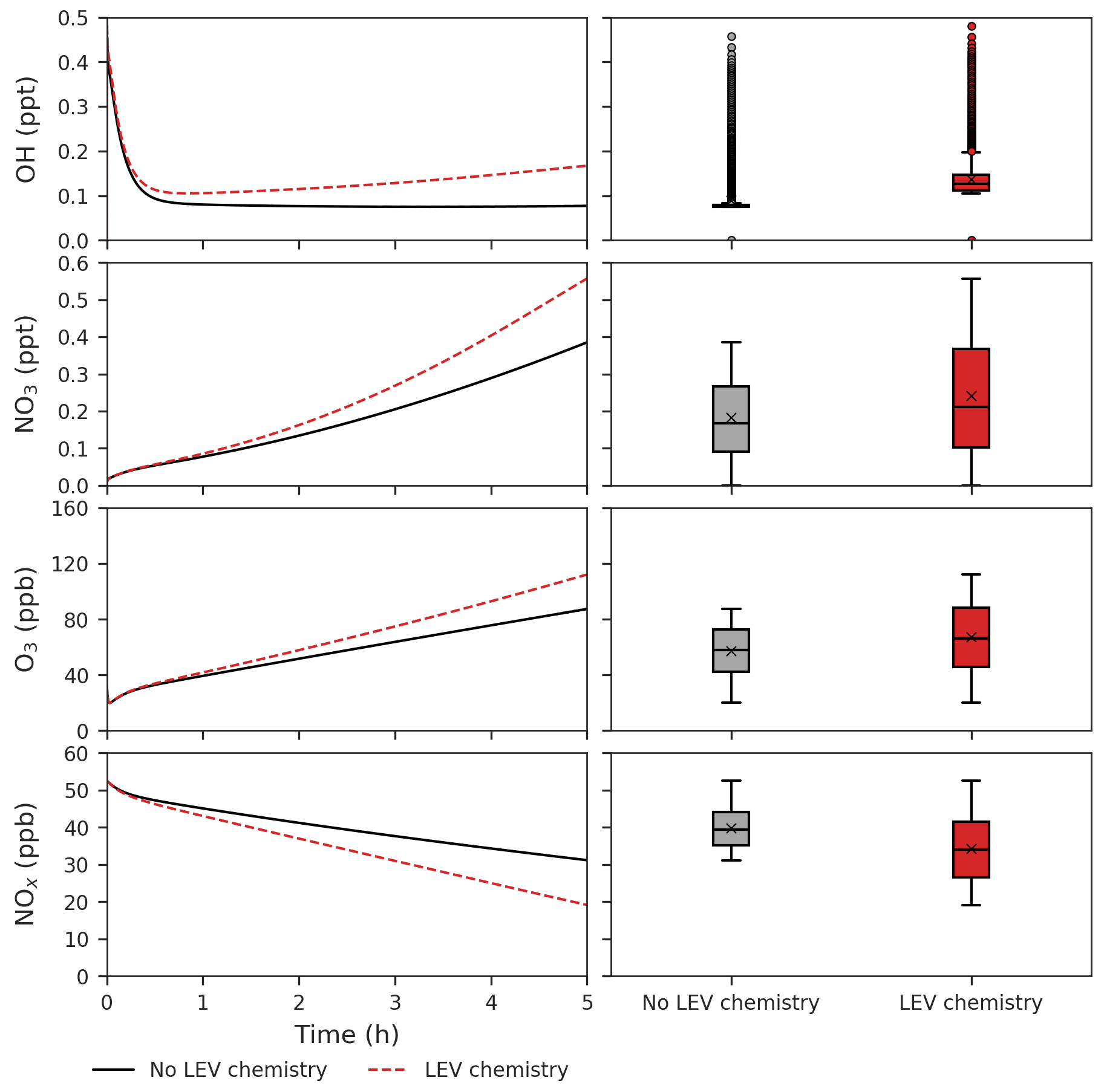
Figure 5 Effects of LEV chemistry on OH, NO₃, O₃ and NO_x (in red, relative to the case without LEV chemistry shown in black or gray). The time series represent averages of simulations performed with LEV chemistry (dashed red line) and without LEV chemistry (black line) over the 5 h timescale. The box plots show the distributions of the species concentration for the entire 5 h. Note that findings shown here are determined over a range of F values depending on experimental conditions.

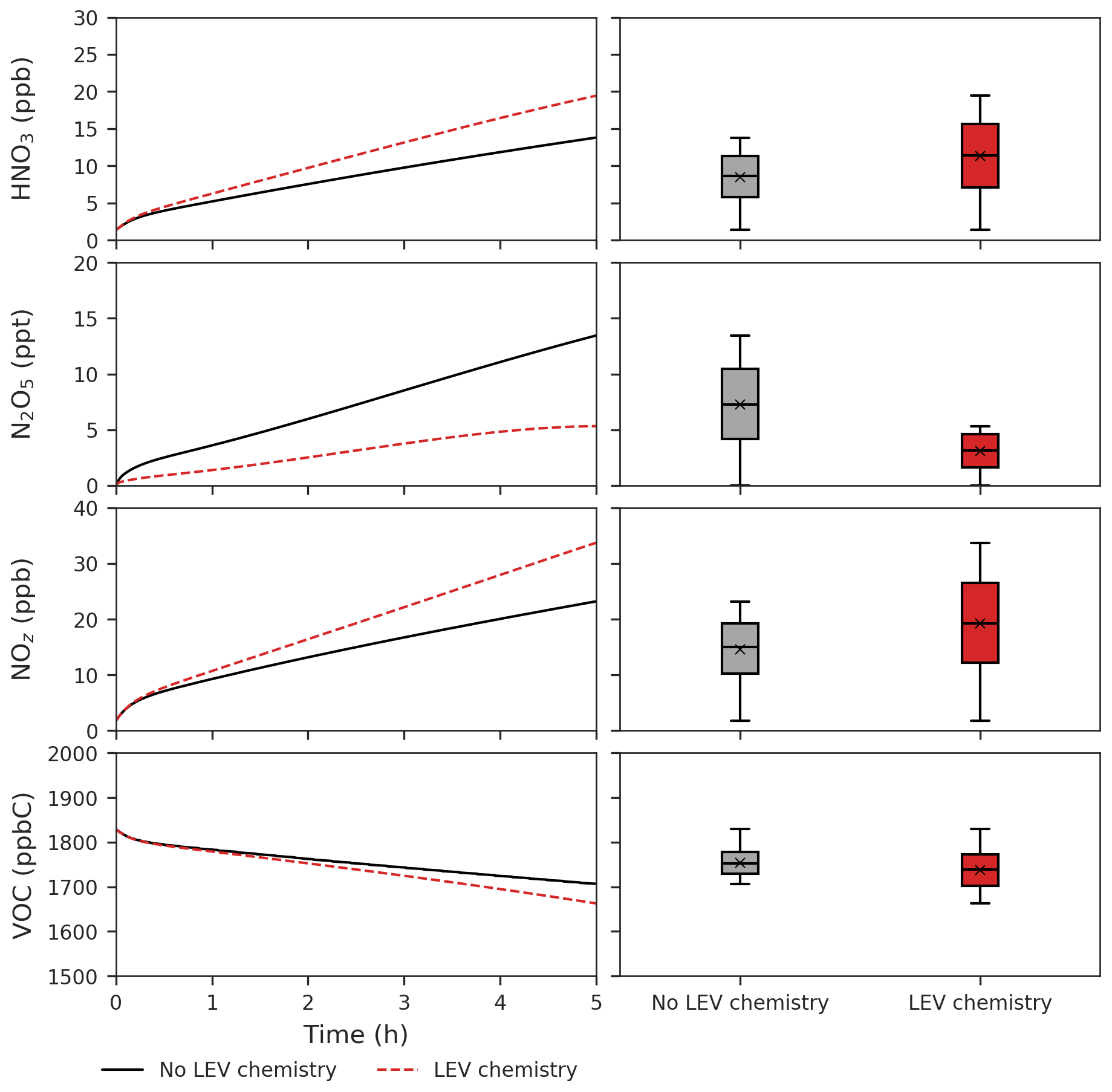
Figure 6 Effects of LEV chemistry on HNO₃, N₂O₅, NO_z and VOCs (in red, relative to the case without LEV chemistry shown in black or gray). The time series represent averages of simulations performed with LEV chemistry (dashed red line) and without LEV chemistry (black line) over the 5 h timescale. The box plots show the distributions of the species concentration for the entire 5 h. Note that findings shown here are determined over a range of F values depending on experimental conditions.

We found that LEV chemistry including G $/$ P partitioning on average increases the concentrations of OH, nitrate radical (NO₃), O₃, nitric acid (HNO₃) and NO_z, whereas it decreases the concentrations of N₂O₅, NO_x and total VOCs (that does not include LEV_G and LEV_A). These effects are the net result of full LEV chemistry in which species may be consumed or generated. For example, OH is consumed in Reactions (R1) and (R10); however, it is also generated directly in Reactions (R4) and (R12) and indirectly through its precursor HO₂ that is generated by Reactions (R3), (R6) and (R12) (Table 1).

LEV chemistry modulates the concentration of reactive species that also interact with other VOCs. Because LEV chemistry increases the concentrations of key oxidants (OH, NO₃, O₃), it causes the concentration of total VOCs to decrease over time due to the increased availability of their oxidants. LEV chemistry also causes NO_z to increase over time; this can mainly be explained by the formation of nitrated organic compounds (LEVP5_G and LEVP5_A) and HNO₃ in Reactions (R13) (Table 1) and (R14) (Table 2). LEV chemistry also generates NO₃ precursors (such as NO₂) that may explain the net increase in the NO₃ concentration (Fig. 5).

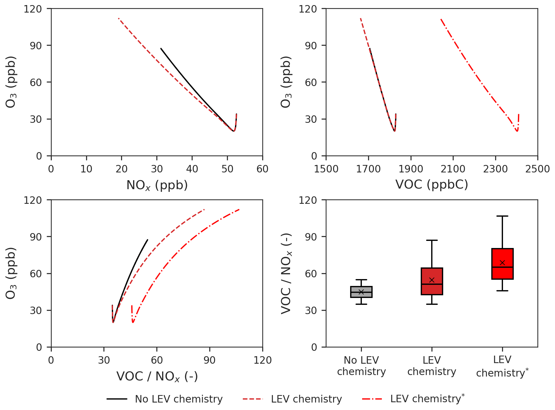
Figure 7 Effects of LEV chemistry on the O₃ vs. NO_x, O₃ vs. VOCs and O₃ vs. $\mathrm{VOC}/{\mathrm{NO}}_x$ ratio relationships and on the $\mathrm{VOC}/{\mathrm{NO}}_x$ ratio. The two cases in red (with LEV chemistry) refer to the two ways in which VOCs were determined (with and without LEV_G and LEV_A). The asterisk refers to the inclusion of LEV_G and LEV_A in the total VOCs. All of the plots show simulation results at the 5 h timescale. Note that findings shown here are determined over a range of F values depending on experimental conditions.

We also studied the effects of LEV chemistry on the O₃ vs. NO_x, O₃ vs. VOCs and O₃ vs. $\mathrm{VOC}/{\mathrm{NO}}_x$ ratio relationships as well as effects on the $\mathrm{VOC}/{\mathrm{NO}}_x$ ratio itself (Fig. 7). While the decay of NO_x slowed down the increase of O₃, the decay of VOCs had no effect on the rate of O₃ formation when total VOCs did not contain LEV_G and LEV_A. When the latter two were included in total VOCs, the decay of total VOCs also reduced the rate of the O₃ increase (linear slope of $-\mathrm{0.250}\pm \mathrm{0.001}$ ppb ppbC⁻¹) but not as much as NO_x did (linear slope of $-\mathrm{2.821}\pm \mathrm{0.007}$ ppb ppb⁻¹). The $\mathrm{VOC}/{\mathrm{NO}}_x$ ratio increases when LEV chemistry is considered, driving O₃ to reach higher concentrations (112 ppb) compared with the default case (without LEV chemistry). Thus, when LEV chemistry operates in the system, the change in the O₃ concentration is primarily driven by the change in NO_x and only secondarily by the change in VOCs.

3.4 Sensitivity analysis

Heterogeneous chemistry is the most sensitive aspect of the modeling approach in the present study. Here, we assumed that the aerosol surface is composed of pure LEV and there are many factors that can interfere or inhibit heterogeneous chemistry of a pure LEV substrate (Sect. 2.3). These controls were lumped into a single factor (F) that we varied from a default case (1.0) to cases in which heterogeneous chemistry was up to 3 orders of magnitude slower. While available chamber experiment studies offered the opportunity to evaluate LEV degradation for a given heterogeneous reaction rate coefficient that was reduced by certain F values (see Sect. 3.1), other values of F are plausible. As a starting point, here we show how these F values influence the degradation timescale of LEV (Fig. 8) and the SOA yields (Fig. 4b). Within this wide range of heterogeneous reaction rates (at constant α=0.1), the degradation timescale of LEV can be as long as 5 d in the gas phase and 7 d in the aerosol phase (when F=0.001). While the timescale of gas-phase LEV is similar (5 d) to that observed with reaction rates used in chamber comparisons (see Sect. 3.1), the timescale of aerosol-phase LEV is much larger (7 d vs. 36 h), suggesting that LEV associated with PM can be transported and deposited regionally. Over these timescales, SOA yields vary roughly within the same range (14 %–33 %) as observed in the previous cases considered (see Sect. 3.2).

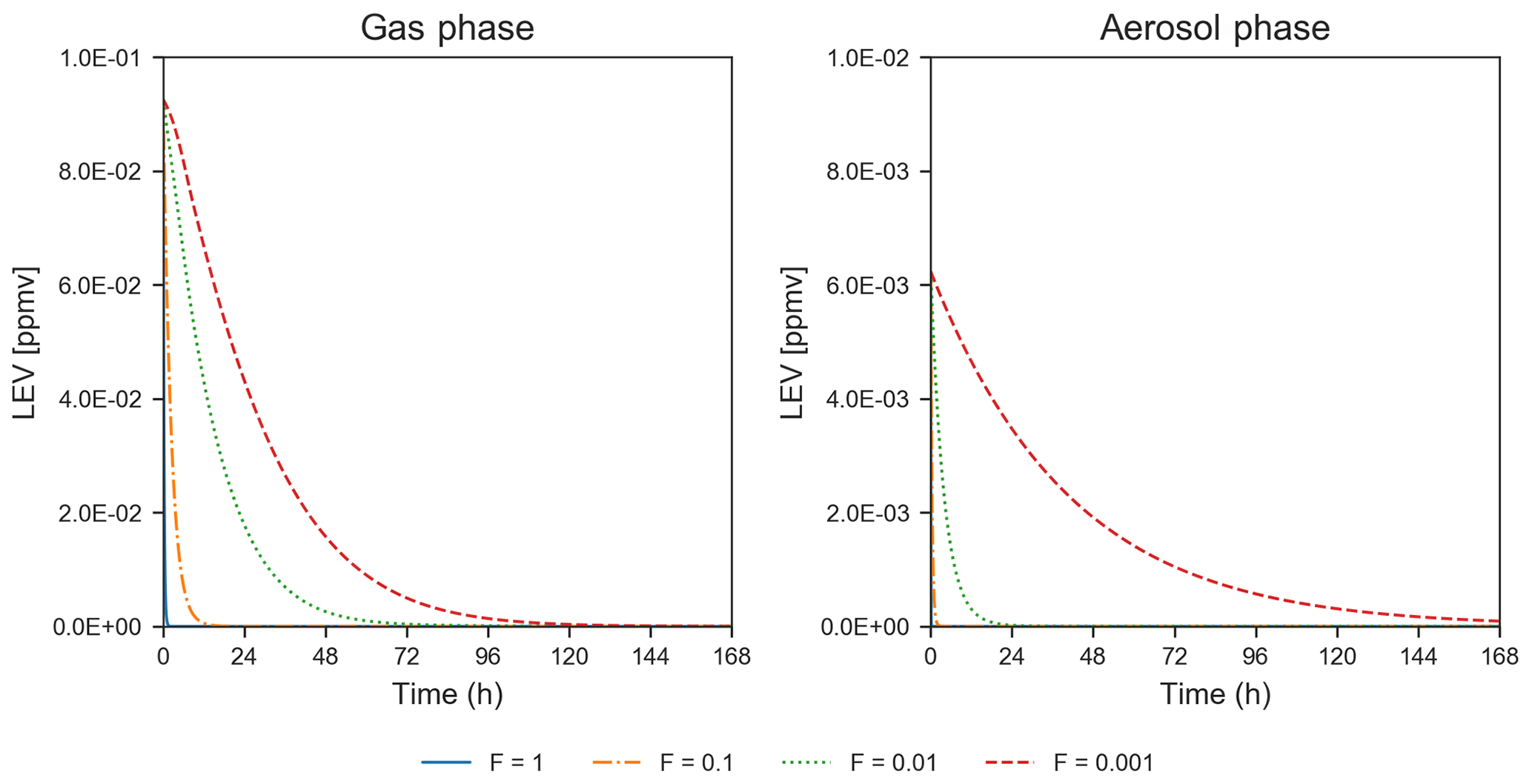
Figure 8 Degradation of LEV by varying the heterogeneous reaction rate coefficient by 4 orders of magnitude, at a constant mass accommodation coefficient (α=0.1) and $C_i^{*}=\mathrm{13}$ µg m⁻³ (conditions from Hennigan et al., 2010). Note that the y axis scale changes between the concentrations presented for the two phases.

We also tested the sensitivity of the mass accommodation coefficient (α) at F=0.01, using conditions from Hennigan et al. (2010). Varying α by 4 orders of magnitude (0.001, 0.01, 0.1 and 1.0) showed little effect on LEV degradation (i.e., degradation in the gas phase was slightly faster when α=1, whereas degradation in the aerosol phase was slightly faster when α=0.001–0.1) in comparison to the effect of slowing down the heterogeneous chemistry (F, as described above). The effect of the mass accommodation coefficient on LEV degradation appears to be more important when the G $/$ P partitioning is modeled as gas-aerosol equilibrium reactions of which the partitioning coefficient is modeled with Eq. (13). This is a different way to implement the G $/$ P partitioning in the model, but it does not drive species phase transfer based on the theoretical surface equilibrium concentration (Eqs. 8, 9).

4 Conclusions

Anhydrosugars emitted by biomass burning are key tracers of PyC and of carbon cycling throughout Earth system reservoirs. However, relatively little is known about their degradation in any environment. A better understanding of the atmospheric degradation of anhydrosugars is necessary for both atmospheric and cryospheric sciences because it will improve the understanding of air quality effects of fire as well as the interpretation of levoglucosan records of fire, paleoclimate and paleovegetation recorded in the ice (Gambaro et al., 2008; Kawamura et al., 2012; Kehrwald et al., 2012; You and Xu, 2018). This study focused on the atmospheric degradation of anhydrosugars from the perspective of LEV, the most abundant anhydrosugar emitted on a mass basis.

Using a 0-D modeling framework (BOXMOXv1.7), we implemented multiphase chemistry and G $/$ P partitioning of LEV and its initial oxidation products (LEVCHEM_v1). We found that LEV degradation timescale ranges from 8–36 h (aerosol-phase) to 1.5–5 d (gas-phase); however, model output was only evaluated for 6 h through comparison to chamber measurements. In addition, we conducted a sensitivity analysis investigating a factor slowing down the heterogeneous chemistry and found that longer degradation timescales may occur, particularly in the aerosol phase (7 d). This longer timescale is slightly larger than that of deposition (1–5 d) but is slightly shorter than that of regional transport (10 d), suggesting that some fraction of aerosol-phase LEV may be transported regionally. However, these timescales remain to be evaluated using more extensive measurements from chambers and fire plumes. Additional sensitivity analyses using larger initial aerosol LEV concentrations in chamber simulations may result in longer degradation timescales of the LEV aerosol concentration. Ultimately, implementation of the 0-D model development of this study into CTMs will help to clarify the regional transport and deposition of both LEV phases.

LEV degradation contributes to SOA formation that was quantified mainly through simulated SOA yields. Based on 6 h degradation timescales, simulated SOA yields ranged from 4 % to 32 % and peaked in the first 2–34 min. Varying the heterogeneous chemistry rate by 4 orders of magnitude did not result in significantly different SOA yields (14 %–33 %). The total PM mass (determined as the ratio of total aerosol concentration to initial LEV_A concentration) increased by 8 %–15 % in the first 6 h of all simulations and continued to slowly increase to 18 %–29 % at the end of the simulation period.

The addition of the multiphase LEV chemistry and the related G $/$ P partitioning mechanism to the 0-D modeling framework has both direct and indirect effects on several gas-phase species. The average concentrations of OH, NO₃, O₃, HNO₃ and NO_z increased, whereas those of N₂O₅, NO_x and other VOCs decreased. These changes are due to chemical reactions of the full LEV chemistry which simultaneously consume and generate reactive species. Other species, included in the total VOCs, are indirectly influenced by the LEV chemistry via competition for oxidants or via the oxidant concentration mediated by LEV chemistry. The effects of LEV chemistry on O₃ are complex: while it slows down its rate of formation by modulating NO_x and VOC concentrations, it increases the $\mathrm{VOC}/{\mathrm{NO}}_x$ ratio, which in turn leads to higher O₃ (112 ppb) compared with the case without LEV chemistry (90 ppb).

LEV chemistry facilitates the conversion of NO_x to other reactive nitrogen forms (an increase of NO_z vs. time at an average NO_z enhancement by 5 ppb). The effects of LEV chemistry on NO_z occur directly through LEVP5, a nitrated organic degradation product, and indirectly via generation of HNO₃ or consumption of N₂O₅, NO and NO₃ in chemical reactions. LEV chemistry drives changes in major air pollutants making it unwise to ignore it in future assessments of fire effects on tropospheric O₃, nitrogen cycling (via NO_z) and carbon cycling (via VOC and aerosol-phase degradation products).

Future work should expand model development to include the degradation of the two LEV isomers (mannosan and galactosan) and to implement the full mechanism of anhydrosugar degradation into 3-D CTMs. The atmospheric implications of anhydrosugar degradation (i.e., SOA formation) and their tracing potential could then be evaluated more completely.