OMEN-SED(-RCM) (v1.1): a pseudo-reactive continuum representation of organic matter degradation dynamics for OMEN-SED

The Organic Matter ENabled SEDiment model (OMEN-SED) is a one-dimensional, analytical reaction–transport model for early diagenesis in marine sediments. It explicitly resolves organic matter (OM) degradation and associated biogeochemical terminal electron acceptor, reduced species and nutrient dynamics in porous media under steady-state conditions. OMEN-SED has been specifically designed for coupling to global Earth system models and the analytical solution of the coupled set of mass conservation equations ensures the computational efficiency required for such a coupling. To find an analytical solution, OMEN-SED expresses all explicitly resolved biogeochemical processes as a function of OM degradation. The original version of OMEN-SED contains a relatively simple description of OM degradation based on two reactive OM classes, a so-called 2G model. However, such a simplified approach does not fully account for the widely observed continuous decrease in organic matter reactivity with burial depth/time. The reactive continuum model that accounts for the continuous distribution of organic compounds over the reactive spectrum represents an alternative and more realistic description but cannot be easily incorporated within the general OMEN-SED framework. Here, we extend the diagenetic framework of OMEN-SED with a multi-G approximation of the reactive continuum model (RCM) of organic matter degradation by using a finite but large number of OM fractions, each characterized by a distinct reactivity. The RCM and its multi-G approximation are fully constrained by only two free parameters, a and ν, that control the initial distribution of OM compounds over the reactivity spectrum. The new model is not only able to reproduce observed pore water profiles, sediment–water interface fluxes and redox zonation across a wide range of depositional environments but also provides a more realistic description of anaerobic degradation pathways. The added functionality extends the applicability of OMEN-SED to a broader range of environments and timescales, while requiring fewer parameters to simulate a wider spectrum of OM reactivities.

1 Introduction

The degradation of organic matter (OM) in marine sediments is a key component of the global carbon cycle and climate (Berner, 1991; Archer and Maier-Reimer, 1994; Ridgwell and Zeebe, 2005). It is the main engine behind the complex and dynamic network of biogeochemical reactions in marine sediments and, thus, controls benthic carbon and nutrient recycling, as well as carbon burial (e.g. Arndt et al., 2013; LaRowe et al., 2020b). As a consequence, it exerts an important influence on marine primary production, the strength of the primary long-term sink for atmospheric CO₂ and, ultimately, the size of the largest carbon reservoir within the Earth system (e.g. Berner, 1980; Soetaert et al., 2000; Aller, 2014; Hülse et al., 2017; LaRowe et al., 2020a). Understanding, quantifying and predicting organic matter degradation and associated biogeochemical dynamics in marine sediments is thus critical for our ability to understand past, present and future biogeochemical cycles and climate dynamics.

Benthic biogeochemical dynamics are driven by a complex and dynamic interplay of transport and reaction processes that operate over different temporal and spatial scales. This underlying complexity compromises our ability to understand, quantify and predict diagenetic dynamics. In this respect, reaction–transport models (RTMs) that account for transport (advection, molecular diffusion, bioturbation and bioirrigation) and reaction (production and consumption) processes are, in combination with observational data, powerful analytic, diagnostic and predictive tools. Because of its prominent role, the description and parametrization of OM degradation in diagenetic models is critical for their ability to capture and predict sediment–water exchange and burial fluxes. The rate of OM degradation and thus the intensity of the associated biogeochemical cycling is first and foremost driven by the supply of OM at the sediment–water interface. However, it is not only the quantity of that flux that determines benthic biogeochemical rates but also its quality (Middelburg et al., 1993; Arndt et al., 2013; LaRowe et al., 2020b). In particular, the benthic redox zonation and benthic recycling fluxes are largely driven by the susceptibility of OM to microbial degradation (Freitas et al., 2021).

Existing OM degradation models can be broadly divided into two different classes according to their description of apparent reactivity of the bulk OM, k(t), and its evolution over time which depends on a complex and dynamic interplay of many different factors (Arndt et al., 2013). Discrete models, also called multi-G models, divide the bulk OM into several discrete fractions, OM_i, each characterized by a different reactivity, k_i (Berner, 1980; Jørgensen, 1978). The apparent reactivity of the bulk OM, k(t), and its evolution over time is then given by the weighted sum of the individual reactivities k_i:

$$\begin{array}{}\text{(1)}& k\left(t\right)=\sum _i{k}_i\cdot {\displaystyle \frac{{\mathrm{OM}}_i\left(t\right)}{{\mathrm{\Sigma }}_i{\mathrm{OM}}_i\left(t\right)}}.\end{array}$$

OM is degraded according to first-order degradation kinetics and the change in OM concentration with burial time/depth is thus given by

$$\begin{array}{}\text{(2)}& {\displaystyle \frac{\mathrm{dOM}}{\mathrm{d}t}}=-k\left(t\right)\cdot \mathrm{OM}\left(t\right)=-\sum _i{k}_i\cdot {\mathrm{OM}}_i\left(t\right).\end{array}$$

Continuum models, on the other hand, assume a continuous distribution of OM compounds over the reactivity spectrum, thus avoiding the need to partition the bulk material into a limited number of discrete compound classes. One can distinguish theoretically derived continuum models (Boudreau and Ruddick, 1991) and empirically derived power laws (Middelburg, 1989) that are mathematically equivalent (Tarutis, 1993; Jørgensen, 1978; Middelburg, 1989). Although the initial distribution of OM compounds cannot be inferred from observations, widely used continuum models, such as the reactive continuum model (RCM; see Boudreau and Ruddick, 1991), apply a gamma distribution because of its mathematical flexibility and its ability to capture observed OM degradation dynamics. Several other functions have been suggested as alternatives, such as the beta distribution (Vähätalo et al., 2010) or the lognormal function (Rothman and Forney, 2007), but eventually all lead to similar OM degradation kinetics (Vähätalo et al., 2010; Boudreau and Arnosti, 2008), despite the different mathematical expressions.

The application of continuum models in the framework of local, one-dimensional diagenetic models is straight forward as these models generally solve the coupled reaction–transport equations numerically. However, computational power rapidly becomes a limiting factor if a coupled set of reaction–transport equations were to be numerically solved on a global scale and over longer timescales. Therefore, global diagenetic models designed for large-scale applications and the coupling to Earth system models are generally either highly simplistic, limited in their scope or rely on the analytical solution of the reaction–transport equation (Hülse et al., 2017, 2018). However, finding an analytical solution for complex reaction networks and depth-varying parameters is difficult and requires several simplifying assumptions. For instance, the recently developed one-dimensional and numerically efficient diagenetic model, Organic Matter ENabled SEDiment model (OMEN-SED), assumes steady-state conditions and accounts for depth changes in parameters and reaction processes by dividing the sediment into a set of discrete yet dynamic biogeochemical zones (Hülse et al., 2018). The considered diagenetic processes are either expressed as a function of OM degradation or as zero- or first-order reactions. In OMEN-SED (Hülse et al., 2018), the bulk OM degradation is described by a multi-G model (i.e. as a sum of first-order degradation rate laws). Consequently, related biogeochemical processes, such as different metabolic pathways, can be expressed as a series of exponential terms (i.e. the analytical solution of the OM conservation equation), for which a general analytical solution can be easily found (Hülse et al., 2018). However, the key limitation of such a multi-G type approach is that it converges to a constant apparent OM reactivity at depth and thus fails to capture the widely observed continuous decrease in OM reactivity with burial time/depth (Middelburg and Meysman, 2007). Although this limitation can be somewhat mitigated by introducing a larger number of compound classes, each new compound class i requires constraining two new parameters (k_i and OM_i). Yet, because of the difficulty associated with identifying discrete classes based on available observation data, the total number of classes that can be reasonably well constrained is typically restricted to a maximum of three (Jørgensen, 1978; Middelburg, 1989). In addition, due to the lack of a theoretical framework that would allow to constrain OM reactivity on a global scale, the choice of OM degradation model parameters k_i and OM_i is particularly challenging for global-scale applications (Hülse et al., 2018). Reported degradation rate constants in marine sediment have been shown to vary by about 10 orders of magnitude (Middelburg et al., 1993; Arndt et al., 2013). Their spatial variability on the global scale, as well as their response to changing environmental conditions over, for instance, past extreme climate events or to projected climate change, is largely unknown. Furthermore, the timescales of OM degradation in the water column (days to weeks) are vastly different than those found in marine sediments (10–10⁶ years). Consequentially, model parameters of OM degradation cannot be directly inferred from the pelagic parametrization. The selected discrete OM pools of the pelagic model are optimized for the representation of OM degradation dynamics on short timescales and can thus not be applied to describe the slower, long-term OM degradation dynamics in the underlying sediment (Hülse et al., 2018).

Continuum models, on the other hand, merely require constraining the two free parameters that define the shape of the initial distribution and the continuous decrease of OM reactivity with time/depth. Therefore, the RCM approach captures a wider range of OM reactivity scenarios over both short and long timescales, while using fewer parameters than multi-G models (Middelburg, 1989; Jørgensen, 1978), since multi-G models, with i fractions, generally require the specification of $\mathrm{2}\cdot i-\mathrm{1}$ parameters (the reactivity and the relative size for the n OM classes) and are thus generally over-parameterized and difficult to constrain on a global scale. In addition, the RCM captures the widely observed continuous decrease in OM reactivity with burial time/depth, while the 2G model converges to a constant apparent OM reactivity at depth (when the reactive OM pool is consumed). Finally, the RCM is in better agreement with our theoretical and qualitative understanding of the OM degradation process (Aller and Blair, 2006), its reactivity and its evolution during burial. This continuous decrease in OM reactivity with time/depth is fully consistent with observations in lakes, soils, lacustrine and marine sediments (Middelburg, 1989; Boudreau and Ruddick, 1991; Forney and Rothman, 2012; Manzoni et al., 2009; Katsev and Crowe, 2015; Mostovaya et al., 2017). For these reasons, continuum models are better suited for global-scale applications, greater sediment depths or longer timescales. However, while these applications of a RCM approach in a global diagenetic model designed for large-scale applications and the coupling to Earth system models would ease the model parametrization requirements, the RCM cannot be directly applied in OMEN-SED, since OMEN-SED's analytical solution relies on the exponential decrease of OM concentration (see Hülse et al., 2018, for details).

In order to extend OMEN-SED with a second OM degradation model, here we developed a multi-G approximation of the RCM and directly integrated it into the mathematical framework of OMEN-SED. We first provide a short summary of OMEN-SED, including a description of the general model approach and the generic algorithm used to match internal boundary conditions and to determine the integration constants for the analytical solutions. We provide a detailed description of the newly integrated RCM approximation for organic matter degradation, followed by an evaluation of the performance of OMEN-SED-RCM by (1) comparing simulated depth profiles of OM, terminal electron acceptors (TEAs) and metabolic byproducts with observations from selected sites, as well as (2) benthic exchange fluxes of TEAs along a global ocean depth transect. In addition to the model–data comparison, OMEN-SED-RCM results are also compared with original OMEN-SED simulation results. We then force OMEN-SED-RCM with global observational data sets of sediment surface OM contents and bottom water concentrations to explore global patterns of O₂ penetration depths and benthic–pelagic exchange fluxes of O₂. Finally, to evaluate the performance of OMEN-SED-RCM in reproducing diagenetic dynamics in the deeper anoxic sediment, we use OMEN-SED-RCM to explore the response of the sulfate–methane transition zone to changes in OM reactivity (i.e. RCM parameter a) and sedimentation rate.

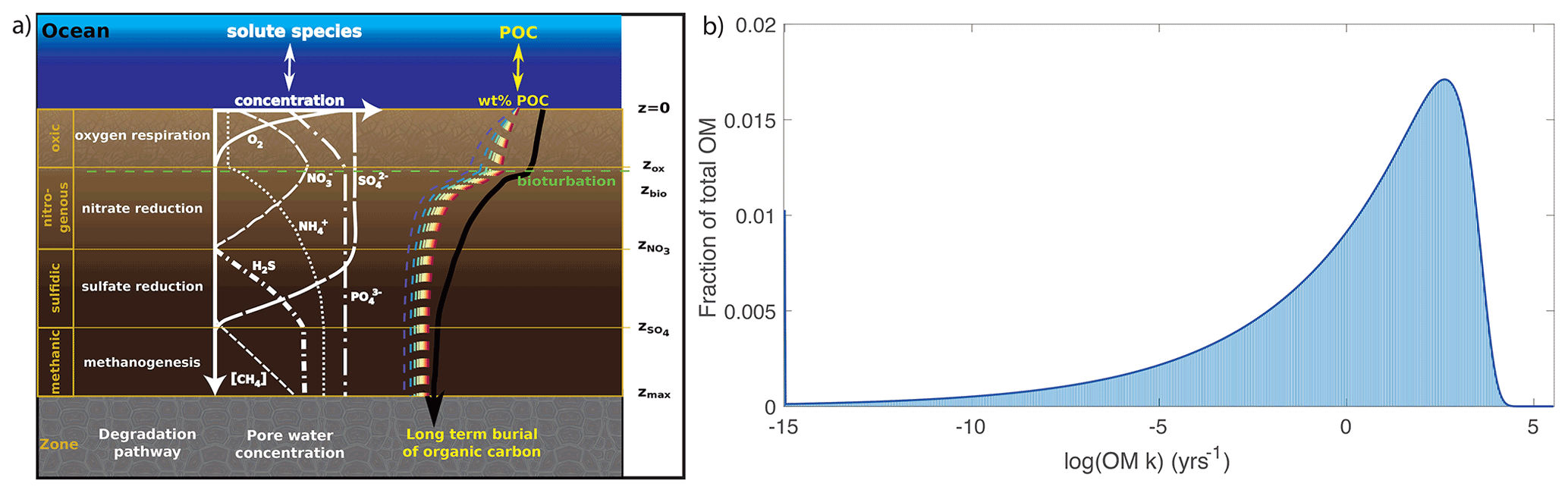
Figure 1 (a) Illustration of the different modelled species and redox zones resolved in OMEN-SED, here showing the case of $z_{ox}<z_{\mathrm{bio}}<z_{{\mathrm{NO}}_{\mathrm{3}}^{-}}<z_{{\mathrm{SO}}_{\mathrm{4}}^{\mathrm{2}-}}$. The black line represents the depth profile of bulk OM concentration, which is the sum of all OM fractions, i (coloured lines) (adapted from Hülse et al., 2018); (b) approximation of the reactive continuum model (continuous dark blue line) with a 500-G model (light blue bars).

2 Model description

OMEN-SED-RCM is based on the diagenetic model OMEN-SED. Hülse et al. (2018) provides a detailed description and evaluation of OMEN-SED. Briefly, OMEN-SED simulates benthic uptake, recycling and burial fluxes based on the vertically resolved conservation equation for solid and dissolved species in porous media (e.g. Berner, 1980; Boudreau, 1997):

$$\begin{array}{}\text{(3)}& {\displaystyle \frac{\partial \mathit{\xi }{C}_i}{\partial t}}=-{\displaystyle \frac{\partial }{\partial z}}\left(-\mathit{\xi }{D}_i{\displaystyle \frac{\partial C_i}{\partial z}}+\mathit{\xi }w{C}_i\right)+\mathit{\xi }\sum _j{R}_i^j,\end{array}$$

where C_i is the concentration of biogeochemical species i, ξ equals the porosity ϕ for solute species (which is defined as $\mathit{\varphi }=\frac{\text{volume porewater}}{\text{volume porewater}+\text{solid sediment}}$) and (1−ϕ) for solid species. The term z denotes the sediment depth, t is the time, w is the sedimentation rate, D_i is the apparent diffusion coefficient of dissolved species i, and ${\sum }_j{R}_i^j$ represents the sum of all biogeochemical rates j affecting species i.

OMEN-SED accounts for both the advective and diffusive transport of dissolved and solid species. Sedimentation is simulated as a constant rate, w, and neglects the effect of sediment compaction (i.e. $\frac{\mathrm{d}\mathit{\varphi }}{\mathrm{d}z}=\mathrm{0}$) due to mathematical constraints (see Hülse et al., 2018). Fick's law of molecular diffusion describes the transport of dissolved species with a species-specific apparent diffusion coefficient D_mol,i. The effect of bioturbation is parameterized by a diffusive term (Boudreau, 1996) with a constant bioturbation coefficient D_bio within the bioturbated zone (z≤z_bio). The reaction network implemented in OMEN-SED accounts for the most important primary and secondary redox reactions, equilibrium reactions, mineral dissolution and precipitation. Adsorption and desorption processes associated with OM degradation dynamics that affect dissolved and solid species are also explicitly resolved in the model. The resulting set of non-linear, depth-varying coupled equations can per se only be solved numerically. To find an analytical solution, OMEN-SED assumes steady-state conditions and expresses all explicitly resolved biogeochemical processes as a function of OM degradation, as zero- or first-order reactions. In addition, it divides the sediment into a bioturbated (z<z_bio) and a non-bioturbated zone (z_bio≤z), as well as an superimposed set of discrete yet dynamic redox zones (Hülse et al., 2018): (1) an oxic zone ($\mathrm{0}<z\le z_{\mathrm{ox}}$); (2) a denitrification (or nitrogenous) zone ($z_{\mathrm{ox}}<z\le z_{{\mathrm{NO}}_{\mathrm{3}}}$); (3) a sulfate reduction zone ($z_{{\mathrm{NO}}_{\mathrm{3}}}<z\le z_{{\mathrm{SO}}_{\mathrm{4}}}$); and finally, (4) a methanogenic zone ($z>z_{{\mathrm{SO}}_{\mathrm{4}}}$) (Fig. 1). OMEN-SED allows bioturbation to occur in the anoxic zones of the sediment (here all zones z>z_ox are combined) and so does not limit the maximum bioturbation depth to be restricted to a specific redox zone. The extent of each redox zone is dynamic, and the depth of each redox boundary varies in response to changes in ocean boundary conditions and forcing. The zones are interlinked by imposing continuity in concentrations and fluxes at the dynamic internal boundaries (z_b ∈ {z_bio, z_ox, $z_{{\mathrm{NO}}_{\mathrm{3}}}$, $z_{{\mathrm{SO}}_{\mathrm{4}}}$} compare, e.g. Ruardij and Van Raaphorst, 1995; Billen, 1982). The general equation, Eq. (3), is applied to each redox zone with depth invariant parameters, but parameters and the formulation of the reaction term (${\sum }_j{R}_i^j$) in Eq. (3) can vary between the redox zones. A thorough explanation of how to solve the dynamically changing penetration depth is given in Hülse et al. (2018) in Sect. 2.3.1 (p. 2661) and is exemplified in Sect. 2.2.4 (p. 2657). OMEN-SED only resolves the most pertinent reaction process within each redox zone and thus simplifies the mathematical description of the reaction network, while retaining its biogeochemical complexity (Hülse et al., 2018).

Here, we extend the 2G-model description of OM degradation incorporated in the original version of OMEN-SED (v. 1.0) with a multi-G approximation of the RCM. This new version, OMEN-SED-RCM, accounts for a continuous yet dynamic distribution of OM compounds over a range of reactivities and captures the widely observed, continuous decrease in apparent OM reactivity with depth/burial age (Boudreau and Ruddick, 1991, and see Fig. 1) and describes the degradation rate of organic matter, R_OM, as

$$\begin{array}{}\text{(4)}& R_{\mathrm{OM}}=-\underset{\mathrm{0}}{\overset{\mathrm{\infty }}{\int }}k\cdot om(k,t)\mathrm{d}k,\end{array}$$

where om(k,t) denotes the amount and initial distribution of bulk OM characterized by a reactivity between k and k+dk at time t, and k (yr⁻¹) being analogous to a reaction rate constant. The initial distribution of organic compounds, om(k,0) for t=0, may take different mathematical forms and cannot be inferred by observations, however a gamma function is often used due to its mathematical properties (Boudreau and Ruddick, 1991, following Aris, 1968 and Ho and Aris, 1987). Assuming first-order degradation kinetics, the initial (t=0) distribution of om over k is given by

$$\begin{array}{}\text{(5)}& om(k,\mathrm{0})=\mathrm{OM}\left(\mathrm{0}\right)\cdot {\displaystyle \frac{a^{\mathit{\nu }}\cdot k^{\mathit{\nu }-\mathrm{1}}\cdot e^{-a\cdot k}}{\mathrm{\Gamma }\left(\mathit{\nu }\right)}},\end{array}$$

where OM(0) is the initial OM content (at the sediment–water interface, SWI), Γ is the gamma function, a (year) is the average lifetime of the more reactive components of the OM mixture, and ν is a dimensionless parameter determining the shape of the distribution near k=0. The free parameters a and ν completely determine the shape of the initial OM compound distribution over the range of k. They thus control the overall reactivity of the bulk OM and its evolution with depth/burial age. High ν and low a values indicate the presence of highly reactive compounds that get rapidly degraded, leading to a rapid decrease in OM reactivity with depth/time. Low ν and high a values, on the other hand, indicate a dominance of less reactive compounds within the initial distribution, resulting in a lower bulk OM reactivity and a slower decrease in reactivity with depth. Although the choice of the gamma function that describes the initial distribution of OM compounds is partly guided by mathematical experience, it has been shown to capture the widely observed dynamics of OM degradation in marine sediments well (Arndt et al., 2013; Boudreau and Ruddick, 1991), while also acknowledging that in reality, the OM distribution is likely much more complex and that our choice of the specific mathematical approximation represents a necessary simplification in the first place (Boudreau and Ruddick, 1991).

Our RCM approximation by a multi-G description of OM degradation (see Fig. 1b) is constrained by the OMEN-SED framework, which relies on an exponential decrease of OM concentration with depth and requires invariant first-order degradation rate constants. Therefore, OMEN-SED-RCM does not solve the RCM, instead it applies a 500G approximation of the RCM to inform the initial distribution of OM compounds over the reactivity spectrum as calculated by the gamma distribution. The bulk (apparent) OM reactivity k(z) of our RCM approximation varies with depth and is calculated as

$$\begin{array}{}\text{(6)}& k\left(z\right)={\displaystyle \frac{\sum k_i\cdot {\mathrm{OM}}_i\left(z\right)}{\mathrm{OM}\left(z\right)}}.\end{array}$$

In other words, bulk organic matter is represented by a large number of i distinct compound classes, OM_i, each degraded according to a first-order degradation rate constant, k_i. The initial fraction of OM in compound class i, OM_i, and its respective degradation rate constant, k_i, are calculated based on the distribution function, thus determining the amount of OM within a given reactivity range k and k+dk at t=0 (Eq. 4). The evolution of the apparent OM reactivity within the mixed bioturbated zone (and below) is determined by the specific consumption rates, k_i, but also by their transport via bioturbation and advection, thus accounting for the mixing of OM from different layers and ages. Upon leaving the mixed layer, the initial OM distribution, om(k,0) at the SWI will indeed have changed to om(k,t_apparent), where t_apparent is the age of the OM determined by transport and degradation processes, as the most reactive fractions are preferentially consumed. The two free parameters a and ν fully describe the initial distribution of OM_i and k_i, and thus OMEN-SED-RCM only requires defining two parameters instead of the $\mathrm{2}\cdot i-\mathrm{1}$ parameters of the multi-G description.

Based on distribution of om (Eq. 5), the initial amount of OM within a discrete reactivity class k can be calculated as

$$\begin{array}{}\text{(7)}& f(k,\mathrm{0})={\displaystyle \frac{om(k,\mathrm{0})}{\mathrm{OM}\left(\mathrm{0}\right)}}={\displaystyle \frac{a^{\mathit{\nu }}\cdot k^{\mathit{\nu }-\mathrm{1}}\cdot e^{-a\cdot k}}{\mathrm{\Gamma }\left(\mathit{\nu }\right)}}.\end{array}$$

The initial fraction of OM within the reactivity range between 0 and k, i.e. having a reactivity ≤ k at t=0, is then given by integrating Eq. (7), assuming a, ν, k>0:

$$\begin{array}{}\text{(8)}& \begin{array}{rl}F(k,\mathrm{0})& =\underset{\mathrm{0}}{\overset{k}{\int }}f(k,\mathrm{0})\mathrm{d}k=\underset{\mathrm{0}}{\overset{k}{\int }}\left({\displaystyle \frac{om(k,\mathrm{0})}{\mathrm{OM}\left(\mathrm{0}\right)}}\right)\mathrm{d}k\\ & ={\displaystyle \frac{a^{\mathit{\nu }}}{\mathrm{\Gamma }\left(\mathit{\nu }\right)}}\underset{\mathrm{0}}{\overset{k}{\int }}(k^{\mathit{\nu }-\mathrm{1}}\cdot e^{-a\cdot k})\mathrm{d}k\\ & ={\displaystyle \frac{a^{\mathit{\nu }}}{\mathrm{\Gamma }(\mathit{\nu }{)}_{\mathrm{0}}}}[-{\displaystyle \frac{\mathrm{\Gamma }(\mathit{\nu },a\cdot k)\cdot k^{\mathit{\nu }}}{(a\cdot k{)}^{\mathit{\nu }}}}{]}_{\mathrm{0}}^k\\ & =[-{\displaystyle \frac{\mathrm{\Gamma }(\mathit{\nu },a\cdot k)}{\mathrm{\Gamma }\left(\mathit{\nu }\right)}}{]}_{\mathrm{0}}^k=-{\displaystyle \frac{\mathrm{\Gamma }(\mathit{\nu },a\cdot k)}{\mathrm{\Gamma }\left(\mathit{\nu }\right)}}\\ & +{\displaystyle \frac{\mathrm{\Gamma }(\mathit{\nu },\mathrm{0})}{\mathrm{\Gamma }\left(\mathit{\nu }\right)}}=\mathrm{1}-{\displaystyle \frac{\mathrm{\Gamma }(\mathit{\nu },a\cdot k)}{\mathrm{\Gamma }\left(\mathit{\nu }\right)}},\end{array}\end{array}$$

where $\mathrm{\Gamma }(\mathit{\nu },a\cdot k)$ denotes the inverse gamma function and $\mathrm{\Gamma }(\mathit{\nu },\mathrm{0})=\mathrm{\Gamma }\left(\mathit{\nu }\right)$. To ensure a full coverage of the relevant reactivity space, we recommend choosing a reactivity range from $k_{\min }={\mathrm{10}}^{-\mathrm{15}}$ to $k_{\max }={\mathrm{10}}^{-\log \left(a\right)+\mathrm{2}}$, although the lower k_min limit can be adapted to the resolved timescales. In addition, the total reactivity range should be divided into at least i=100 equal reactivity bins to ensure an appropriate approximation of the initial OM distribution in case parameter a≪0.01 (Fig. 2). However, because computational cost is not a limiting factor for OMEN-SED-RCM, a larger number of classes can also be applied. Here, the RCM is approximated by dividing the reactivity range k= [10⁻¹⁵, ${\mathrm{10}}^{-\log \left(a\right)+\mathrm{2}}$] into i=500 equal reactivity bins, each characterized by a different reactivity constant, k_i, thus ensuring a comprehensive approximation of the gamma function defined by the respective a and ν values.

The initial fraction F_i of total OM in compound class i defined by the reactivity bins k_i and k_i+dk_i at t(0):

$$\begin{array}{}\text{(9)}& F_i=F(k_i,\mathrm{0})-F(k_{i-\mathrm{1}},\mathrm{0}).\end{array}$$

The least, F_min = $k_{\min }={\mathrm{10}}^{-\mathrm{15}}$ yr⁻¹, and most reactive fractions, F_max = $k_{\max }={\mathrm{10}}^{-\log \left(a\right)+\mathrm{2}}$ yr⁻¹, are calculated based on the lower and upper incomplete gamma function, respectively:

$$\begin{array}{}\text{(10)}& {\displaystyle }{F}_{\min }=\underset{\mathrm{0}}{\overset{k_{\min }}{\int }}f(k_{\min },\mathrm{0})\mathrm{d}k={\displaystyle \frac{\mathrm{\Gamma }(\mathit{\nu },a\cdot k_{\min })}{\mathrm{\Gamma }\left(\mathit{\nu }\right)}}\text{(11)}& {\displaystyle }{F}_{\max }=\underset{k_{\max }}{\overset{\mathrm{\infty }}{\int }}f(k_{\max },\mathrm{0})\mathrm{d}k={\displaystyle \frac{\mathrm{\Gamma }(\mathit{\nu },a\cdot k_{\max })}{\mathrm{\Gamma }\left(\mathit{\nu }\right)}}.\end{array}$$

The derived degradation rate constants for OM_i, k_i, are then used in the first-order reaction term within the conservation equation for organic matter dynamics (see Hülse et al., 2018, for details about the analytical solution):

$$\begin{array}{}\text{(12)}& {\displaystyle \frac{\partial {\mathrm{OM}}_i}{\partial t}}=\mathrm{0}=D_{{\mathrm{OM}}_i}\cdot {\displaystyle \frac{{\partial }^{\mathrm{2}}{\mathrm{OM}}_i}{\partial z^{\mathrm{2}}}}-\mathit{\omega }{\displaystyle \frac{\partial {\mathrm{OM}}_i}{\partial z}}-k_i\cdot {\mathrm{OM}}_i,\end{array}$$

with OM${}_i=F_i\cdot \mathrm{OM}\left(\mathrm{0}\right)$, $D_{{\mathrm{OM}}_i}=D_{\mathrm{bio}}$ for z≤z_bio and $D_{{\mathrm{OM}}_i}=\mathrm{0}$ for z>z_bio.

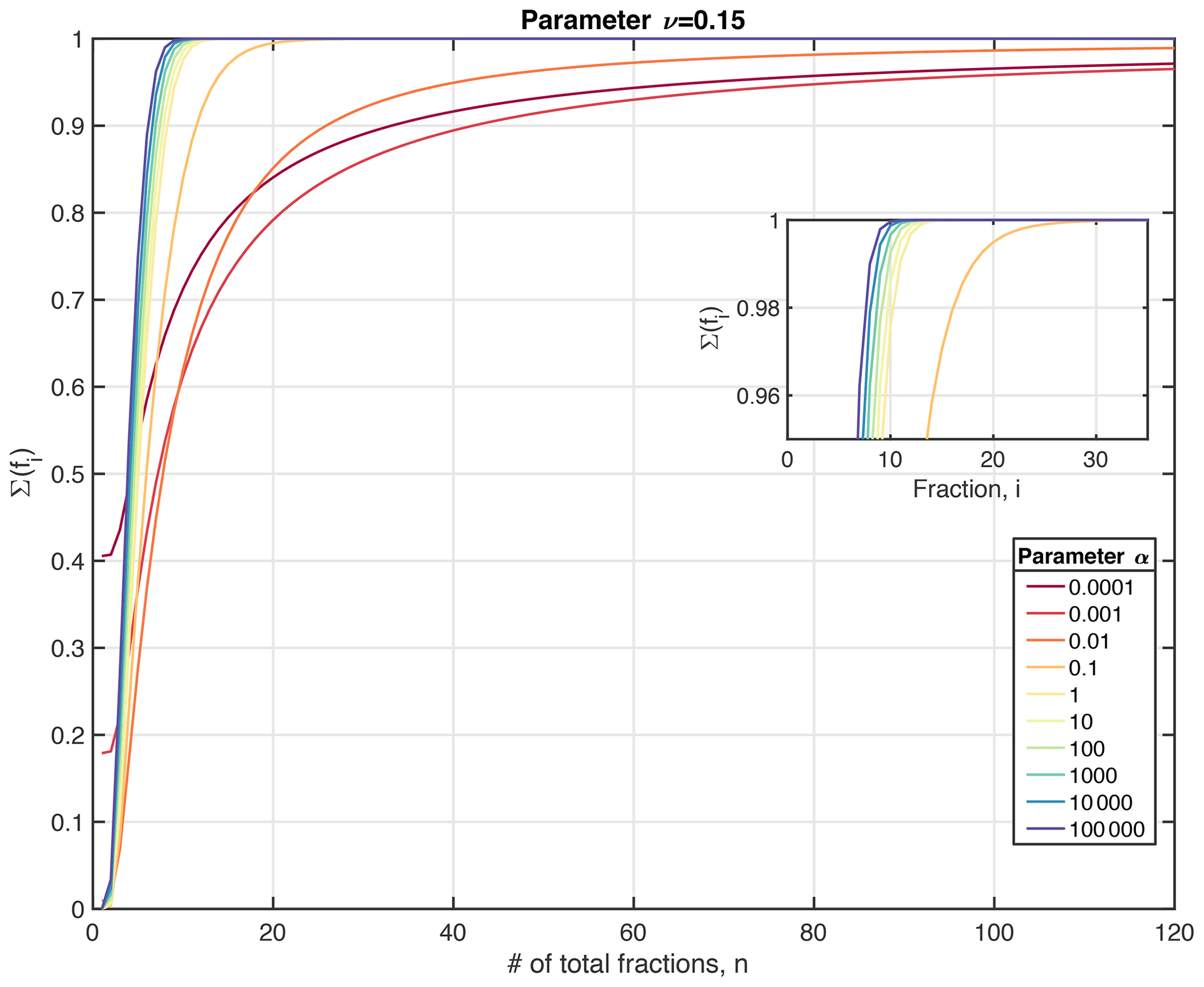
Figure 2 Quality of the multi-G approximation (expressed as the sum of the reactive fractions) as a function of the number of reactivity bins, n, for different RCM parameter a (here shown for ν=0.15). The sum of ∑_i(f_i) should approach 1.0 for an adequate approximation. More reactive OM mixtures (i.e. represented by a small parameter a) require a larger number of fractions n than more unreactive OM mixtures (i.e. a larger parameter a) to achieve a good approximation of the gamma function.

3 Results and discussion

3.1 Case study: sediment core simulations

3.1.1 Methodology

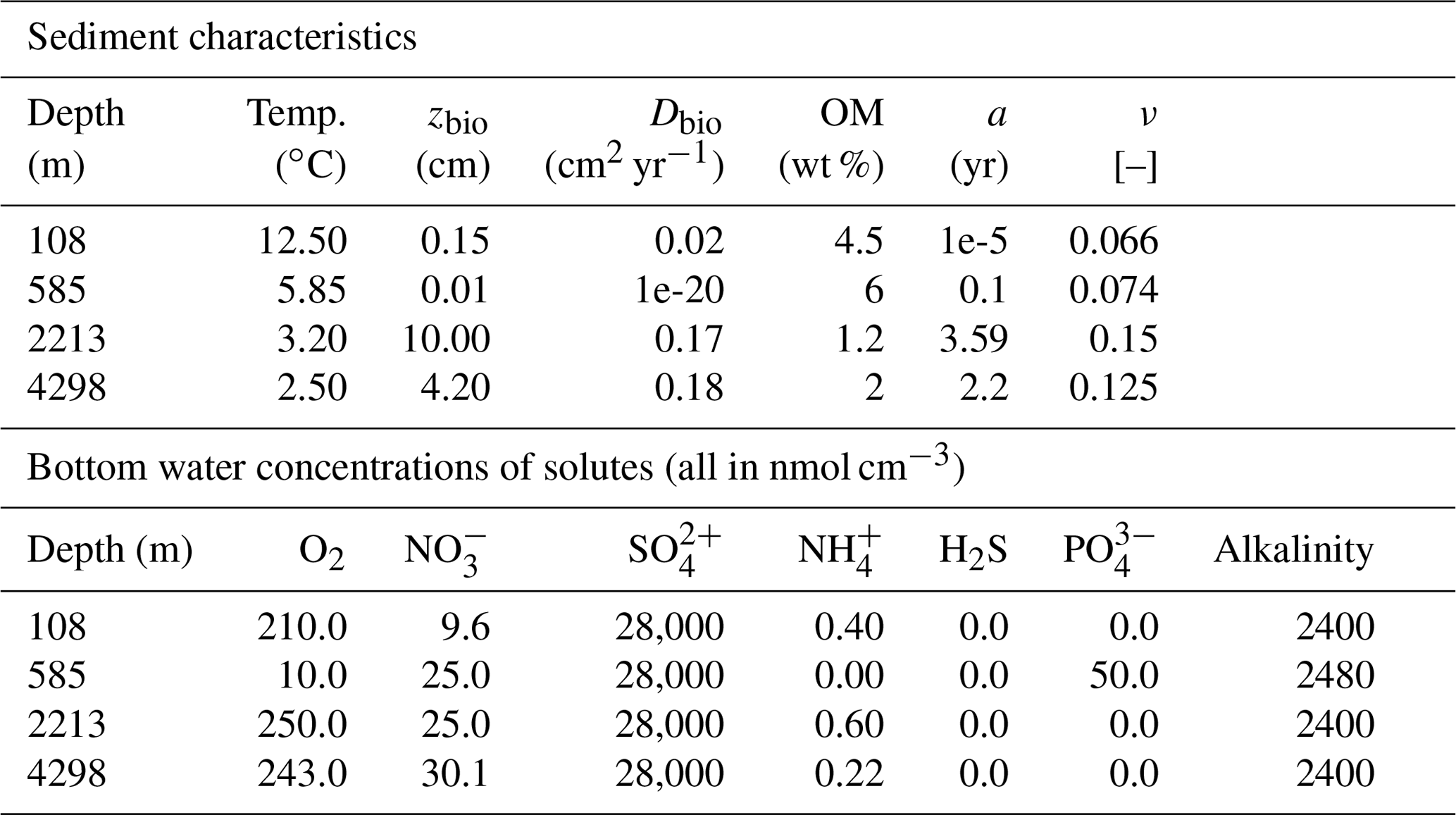
To illustrate the capabilities of OMEN-SED-RCM in simulating local diagenetic dynamics and compare its performance with the original 2G model description implemented in OMEN-SED, we here simulate the simulations for the same four sediment cores that were used to benchmark OMEN-SED (Hülse et al., 2018): Santa Barbara Basin (Reimers et al., 1996), the Iberian margin and Nazaré Canyon (Epping et al., 2002). These simulations cover a wide range of different benthic environments reaching from the shallow shelf to the deep sea, including the highly productive eastern upwelling area on the Iberian Shelf (108 m), the upper slope, organic-rich and non-bioturbated sediments underlying anoxic bottom waters in the Santa Barbara Basin (585 m) and lower slope on the Iberian margin (2213 m), as well as the deep-sea sediments in the Nazaré Canyon (4298 m). For a detailed description of the study sites, see Reimers et al. (1996) and Epping et al. (2002). For this set of simulations, all boundary conditions and parameter values are taken from Hülse et al. (2018), who adapted the boundary conditions and parameter values from the original publications where available or chose the default parameter values set in OMEN-SED, which in turn were constrained based on published values. Table 1 provides the respective boundary conditions used in the simulations. Additional sediment characteristics (e.g. sedimentation rate, porosity, density), stoichiometric factors and secondary reaction parameters are chosen as in Hülse et al. (2018) (see Tables B1 and C1). The free RCM parameters a and ν are the optimized to find the best fit between observations and model results, while all other parameters are kept at their standard value (Hülse et al., 2018).

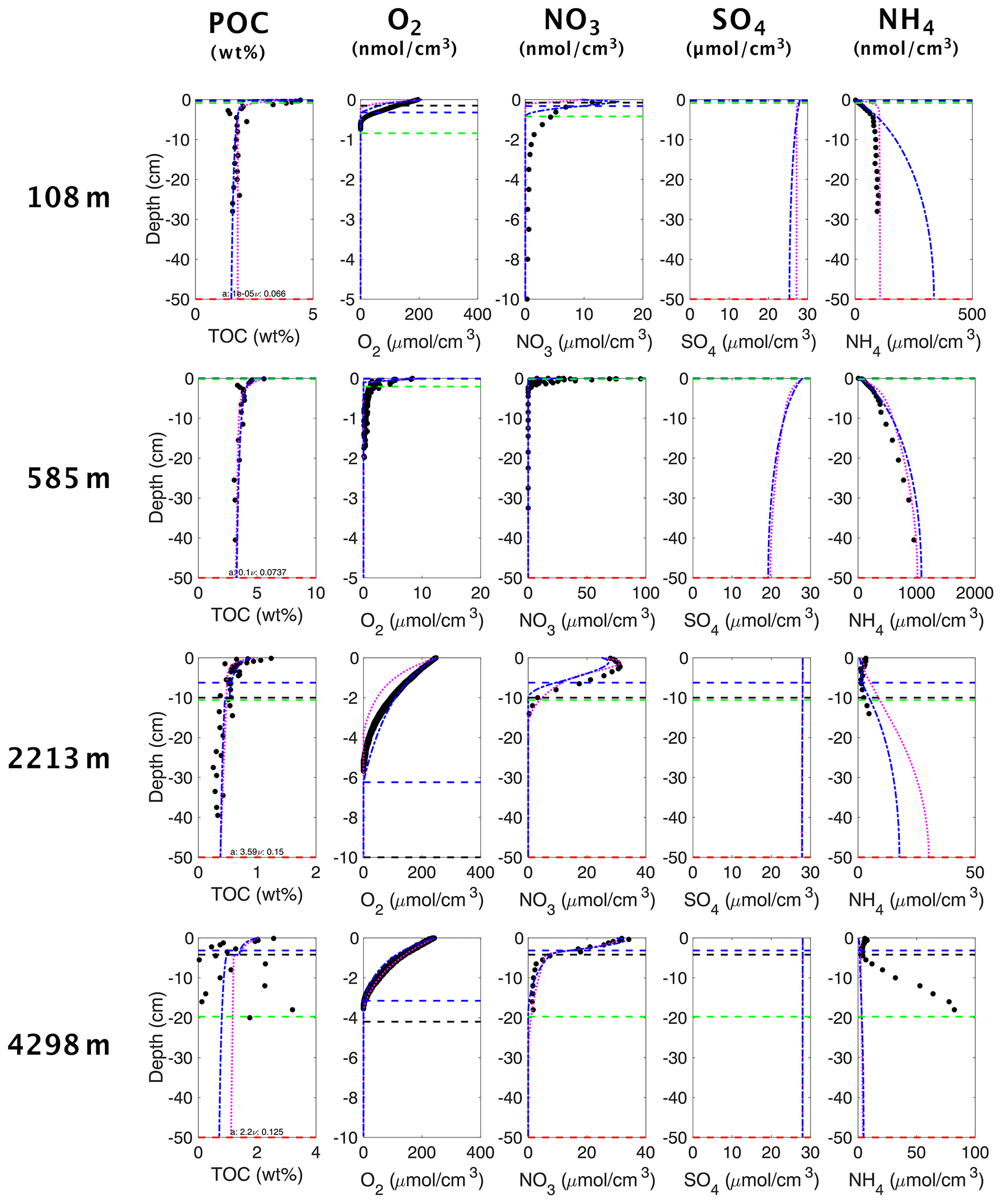
Figure 3 OMEN-SED-RCM (blue curves), 2G OMEN-SED (magenta curves) (Hülse et al., 2018) and observed (filled dots) solid-phase and dissolved pore water profiles for four different sediment cores. Note that different scales are used for different stations. The horizontal dashed lines in each panel indicate the bioturbation depth (black) and the penetration depths of oxygen (blue), nitrate (green) and sulfate (red) as calculated by the updated OMEN-SED.

3.1.2 Results

Figure 3 shows the comparison of simulation results using OMEN-SED-RCM and the original 2G OM model with observed pore water and solid-phase profiles for each of the four case study sites. Results show that, despite the underlying simplifications and the reduced fitting effort, OMEN-SED-RCM captures the main observed diagenetic features across the range of different depositional environments.

More specifically, for the two Iberian margin sites (108 and 2213 m), OMEN-SED-RCM fits observations generally well. A slight overestimation of ${\mathrm{NH}}_{\mathrm{4}}^{+}$ production is simulated for the shallower site. A good agreement between simulation results and observations is also found for the Nazaré Canyon station (4298 m), although simulation results underestimate ${\mathrm{NH}}_{\mathrm{4}}^{+}$ concentrations. The highly variable observed OM depth profile that results from episodic pulses of OM deposition through the canyon could be equally well fit by several different a–ν combinations; none of these combinations produces a better fit of the ${\mathrm{NH}}_{\mathrm{4}}^{+}$ profile. Hülse et al. (2018) invoked a number of factors that compromise the model–data fit of the ${\mathrm{NH}}_{\mathrm{4}}^{+}$ profile at this site. First, Epping et al. (2002), who also did not obtain a better fit with the diagenetic model OMEXDIA, suggest intense bioirrigation activity as a potential driver of higher ${\mathrm{NH}}_{\mathrm{4}}^{+}$ concentrations. Due to mathematical constrains, OMEN-SED merely includes a simplified description of bioirrigation that would require site specific fitting to account for locally enhanced irrigation rates. In addition, Hülse et al. (2018) showed that the model–data fit can be improved by choosing a different nitrogen-to-carbon (NC) ratio and thus reflecting observed variations in Redfield stoichiometries at the Iberian margin and Nazaré Canyon sites (Epping et al., 2002).

Overall, a comparison between OMEN-SED and OMEN-SED-RCM results shows that both models reproduce observations equally well. They mainly differ in simulating the deeper parts of the ${\mathrm{NH}}_{\mathrm{4}}^{+}$ profiles. These differences can be directly linked to the different descriptions of the OM degradation dynamics. While the 2G model formulation (i.e. OMEN-SED) results in an abrupt decrease in OM degradation rates once the more reactive fraction is consumed, the RCM (i.e. OMEN-SED-RCM) accounts for the continuous decrease in OM degradation, thus resulting in a continuous consumption of ${\mathrm{SO}}_{\mathrm{4}}^{\mathrm{2}-}$ and production of ${\mathrm{NH}}_{\mathrm{4}}^{-}$ in the first layers under the SWI.

Finally, inversely fitted OM reactivity parameters a and ν reveal a dominance of highly reactive to reactive OM compounds in the bulk OM across all sites. The consumption of these reactive compounds in the upper sediment layers results in a rapid decrease in apparent OM reactivity with depth for all sites (see Table C1). Even the deep site on the Iberian margin yields a comparably low a value indicating an initial presence of comparably reactive components. This is in line with the comparably high (k=0.1 yr⁻¹) first-order reaction rate constant of the more reactive pool determined by Hülse et al. (2018) and reflects the heterogeneity of OM quality on the spatial scale. Apparent OM reactivity is controlled by a complex interplay of environmental factors and OM deposited at 2000 m depths (or more) and might be as reactive or even more reactive than OM deposited in the shallow ocean (see, e.g. Fig. 15a in Arndt et al., 2013). The Iberian margin is a highly productive and dynamic depositional environment that is characterized by the development of pronounced nepheloid layers in the area Nazaré Canyon (Epping et al., 2002). These nepheloid layers extend to considerably greater water depths and efficiently transport more reactive OM laterally down the slope. Thus the intense lateral transport of OM might explain the occurrence of comparably reactive OM at greater depths. These results are not only fully consistent with the previously determined 2G model parameters (Hülse et al., 2018) but also explain the good performance of the 2G model and the small differences between the RCM and 2G model for these sites. The observed initially high, but rapidly decreasing, OM reactivity can be, in contrast to a more slowly decreasing OM reactivity, adequately reproduced by a 2G model description.

Table 1 Model boundary conditions and parameters for the simulated sediment profiles in Fig. 3 were taken from Hülse et al. (2018), who adapted boundary conditions and parameters from the original publications, except OM reactivity parameters a and ν. For a detailed description of the study sites in the Santa Barbara Basin (108 and 2213 m) and the Iberian margin (585 and 4298 m), see Reimers et al. (1996) and Epping et al. (2002). D_bio at the 585 m site is set to a non-zero value for mathematical reasons.

3.2 Case study: simulation of global ocean transect

3.2.1 Methodology

To evaluate the performance of OMEN-SED-RCM in capturing OM degradation pathways and the resulting TEA fluxes across different depositional environments we replicate the global ocean transect simulation by Thullner et al. (2009). OMEN-SED-RCM simulation results are then compared with global observations but also with results of OMEN-SED (Hülse et al., 2018) and a complex, numerical diagenetic model used in Thullner et al. (2009). Benthic biogeochemical dynamics and exchange TEA fluxes across the SWI are simulated for seven sites situated along the global ocean hypsometry (i.e. seafloor depth (SFD) of 100, 200, 500, 1000, 2000, 3500 and 5000 m). Thullner et al. (2009) used the Biogeochemical Reaction Network Simulator (BRNS, Aguilera et al., 2005), a fully coupled, one-dimensional numerical diagenetic model forced by global observations of bottom water concentrations and fluxes averaged over the respective depth bins. Here, we force OMEN-SED-RCM with the same set of boundary conditions and transport parameters and apply the standard set of OMEN-SED model parameters (Hülse et al., 2018). However, the three applied models differ in their description of OM degradation dynamics. Thullner et al. (2009) and Hülse et al. (2018) apply a simple 1-G model approach, while OMEN-SED-RCM uses the 500-G model approximation of the RCM. Thullner et al. (2009) determined first order degradation rate constants as a function of sedimentation rate for each SFD, following an empirical relationship proposed by Boudreau (1997). They assume that this rate constant is broadly representative of the mean OM reactivity within the upper bioturbated 10–20 cm of the sediments. Hülse et al. (2018) applied the same rate constants in their OMEN-SED simulations. In contrast, our approach constrains the free parameters of the RCM based on a global compilation of previously published values (see Eq. 13 and also Arndt et al., 2013). Inversely determined RCM parameters across a wide range of different environments show that ν mainly falls between 0.1–0.2 (apparent 6th–11th order of reaction), while parameter a varies globally across orders of magnitude (Boudreau and Ruddick, 1991; Arndt et al., 2013; Freitas et al., 2021). Based on these previous global findings, we assume that parameter a controls the global variability in OM reactivity and that parameter ν remains roughly constant at ν=0.15 across different depositional environments. Because parameter a is conceptually related to the average lifetime of the more reactive OM components and, thus, the degree of degradation or freshness of OM, the residence time of OM in the water column should exert, among other factors, a control on its magnitude (Boudreau and Ruddick, 1991; Middelburg, 1989). Boudreau and Ruddick (1991) and Arndt et al. (2013) found, indeed, a weak trend between parameter a and sedimentation rate:

$$\begin{array}{}\text{(13)}& {\text{Log}}_{\mathrm{10}}\left(a\right)=\mathrm{3.35}-\mathrm{14.81}\cdot \mathit{\omega },r^{\mathrm{2}}=\mathrm{0.46}.\end{array}$$

Here, we use this global relationship to estimate parameter a as a function of ω for sites deeper than 200 m water depths along the global hypsometry by expressing ω as a function of SFD using an empirical relationship Middelburg et al. (1997) (see Table 2). For high sedimentation rates, and thus shallow water depths, the limited available data set does not fully cover the variability in OM reactivities that results from the dynamic mix of different OM sources in combination with the complex interplay of different controlling factors, such as physical protection mechanisms, microbial community composition or macrobenthic activity (Arndt et al., 2013). As a result, Eq. (13) tends to underestimate OM reactivity in the coastal ocean. Therefore, we here assume that the shallowest site (SFD of 200 m) has an apparent OM reactivity that is characteristic for fresh phytoplankton (Boudreau and Ruddick, 1991). As a result, apparent OM reactivities along the global ocean transect decreases over six orders of magnitude from the shallowest to the deepest SFD: k=53.09 yr⁻¹ ($a=\mathrm{2.8}\times {\mathrm{10}}^{-\mathrm{3}}$ yr) at 100 m to $k=\mathrm{7.45}\times \mathrm{10}{e}^{-\mathrm{5}}$ yr⁻¹ ($a=\mathrm{2}\times {\mathrm{10}}^{\mathrm{3}}$ yr) at 5000 m, which is similar to the range reported in Arndt et al. (2013). Albeit not directly comparable, due to the different parametrization of the OM degradation rate, the approach by Thullner et al. (2009) assumed a decrease in the overall reactivity over the same depth transect of only 1 order of magnitude.

In addition to OM reactivity, the reoxidation of reduced substances (i.e. ${\mathit{\gamma }}_{{\mathrm{NH}}_{\mathrm{4}}}$, ${\mathit{\gamma }}_{{\mathrm{H}}_{\mathrm{2}}\mathrm{S}}$) substantially affects the simulated benthic fluxes across the SWI. Here, we assume that a fixed fraction of NH₄ and H₂S is oxidized (i.e. ${\mathit{\gamma }}_{{\mathrm{NH}}_{\mathrm{4}}}={\mathit{\gamma }}_{{\mathrm{H}}_{\mathrm{2}}\mathrm{S}}=\mathrm{0.95}$). We acknowledge that choosing a different fraction might change the simulated fluxes, but the resulting range is narrower than the one shown by Hülse et al. (2018) using the 1-G OMEN-SED version (see Fig. 4).

Table 2 Seafloor depth dependency of key model parameters and boundary conditions (adapted from Thullner et al., 2009).

Superscripted numbers denote the following references: ^a Middelburg et al. (1997). ^b Van Cappellen and Wang (1995). ^c Conkright et al. (2002). ^d Boudreau (1997). ^e Calculated with OMEN-SED from OM_flux. ^f Constant value according to Boudreau and Ruddick (1991) and Freitas et al. (2021). ^g Calculated with Eq. (13). ^h Calculated with Eq. (6).

Figure 4 Simulated (lines) and observed (points) benthic fluxes of O₂, ${\mathrm{NO}}_{\mathrm{3}}^{-}$ and ${\mathrm{SO}}_{\mathrm{4}}^{\mathrm{2}-}$ along a global hypsometry transect. Flux units are in µmol cm⁻² yr⁻¹. OMEN-SED-RCM (blue lines with grey squares) are compared to simulation results from the numerical diagenetic model BRNS (red lines with open symbols, Thullner et al., 2009); and results from the analytical diagenetic model OMEN-SED (black lines, •: ${\mathit{\gamma }}_{{\mathrm{NH}}_{\mathrm{4}}}={\mathit{\gamma }}_{{\mathrm{H}}_{\mathrm{2}}\mathrm{S}}=\mathrm{0.95}$; ▾: ${\mathit{\gamma }}_{{\mathrm{NH}}_{\mathrm{4}}}={\mathit{\gamma }}_{{\mathrm{H}}_{\mathrm{2}}\mathrm{S}}=\mathrm{0.05}$), Hülse et al. (2018). The red line with filled circles indicates total oxygen uptake simulated by Thullner et al. (2009). The green line indicates OMEN-SED-RCM simulations that were forced with boundary conditions and N:C values that are more representative of the eastern Pacific Ocean. Observed data of O₂ and ${\mathrm{NO}}_{\mathrm{3}}^{-}$ fluxes from the Atlantic (diamonds), Pacific (squares) and Arctic/Indian oceans (crosses) are from Middelburg et al. (1996), while ${\mathrm{SO}}_{\mathrm{4}}^{\mathrm{2}-}$ data (circles) are from Egger et al. (2018).

3.2.2 Results

Figure 4 compares the results of the simulated benthic TEA fluxes (i.e. O₂, ${\mathrm{NO}}_{\mathrm{3}}^{\mathrm{2}-}$ and ${\mathrm{SO}}_{\mathrm{4}}^{\mathrm{2}-}$) along the global hypsometry using OMEN-SED-RCM (blue lines) with the original 1-G OMEN-SED version (black lines), the simulation results of Thullner et al. (2009) (red lines) and global observations (black dots/squares/diamonds). Model results are compared with observed O₂ and ${\mathrm{NO}}_{\mathrm{3}}^{\mathrm{2}-}$ compiled by Middelburg et al. (1997) and ${\mathrm{SO}}_{\mathrm{4}}^{\mathrm{2}-}$ compiled by Egger et al. (2018). In general, TEA fluxes simulated with OMEN-SED-RCM are lower than OMEN-SED (Hülse et al., 2018) and BRNS (Thullner et al., 2009) simulations (Fig. 4). This difference can be directly attributed to the different representations of OM degradation dynamics in the three models (i.e. numerical 1-G, analytical 1-G and analytical 500-G model RCM approximation). The 1-G model applied by Thullner et al. (2009) and Hülse et al. (2018) assumes a constant OM reactivity for the entire sediment column and therefore overestimates bulk OM reactivity in the deeper, often anoxic, sediment layers, resulting in higher TEA uptake. The RCM approximation, on the other hand, accounts for the entire reactivity continuum and thus captures the decrease in apparent OM reactivity with sediment depth. As a result, OM degradation rates decrease faster with sediment depth, resulting in a reduced TEA uptake.

Figure 4 shows that OMEN-SED-RCM captures the observed decrease in TEA uptake fluxes from the shallow coastal ocean to the deep abyss well. Like the other models, it slightly underestimates observed deep ocean O₂ fluxes (>2000 m). These low O₂ fluxes are a direct consequence of the low OM reactivities (i.e. high parameter a) estimated for these water depths in combination with a potential bias in O₂ uptake flux observations towards more dynamic deep-sea sites that receive by more reactive OM. Equation (13) likely underestimates OM reactivity for the more dynamic deep-sea sites (Arndt et al., 2013), resulting in a slight underestimation of fluxes. Furthermore, OMEN-SED-RCM reproduces the observed water depth trend in ${\mathrm{NO}}_{\mathrm{3}}^{-}$ uptake fluxes well but, like the other models, underestimates the high ${\mathrm{NO}}_{\mathrm{3}}^{-}$ uptake fluxes observed in the shallow Pacific Ocean (Middelburg et al., 1996). As suggested by Hülse et al. (2018), an improved model–data fit (green line) can be obtained by applying boundary conditions (O₂=10 nmol cm⁻³ and ${\mathrm{NO}}_{\mathrm{3}}^{-}=\mathrm{80}$ nmol cm⁻³) and a C:N elemental ratio (C:N ratio is 0.067) that are more representative of the eastern Pacific Ocean (see Bohlen et al., 2012). Finally, OMEN-SED-RCM also captures the observed trend in ${\mathrm{SO}}_{\mathrm{4}}^{\mathrm{2}-}$ uptake fluxes well. Simulation results also agree well with OMEN-SED results that assume an almost complete re-oxidation of the deep H₂S flux (i.e. ${\mathit{\gamma }}_{{\mathrm{H}}_{\mathrm{2}}\mathrm{S}}=\mathrm{95}$ % black line with black circle, hidden by the OMEN-SED-RCM results). In contrast, BRNS model results, as well as OMEN-SED results, that assume a weak re-oxidation of the deep H₂S flux (i.e. ${\mathit{\gamma }}_{{\mathrm{H}}_{\mathrm{2}}\mathrm{S}}=\mathrm{0.05}\mathit{\%}$ (black line with black triangles) also both overestimate anoxic OM degradation and thus ${\mathrm{SO}}_{\mathrm{4}}^{\mathrm{2}-}$ uptake flux. Yet, like the high ${\mathrm{NO}}_{\mathrm{3}}^{-}$ uptake fluxes observed in the shallow Pacific Ocean, all model simulations fail to capture locally observed high ${\mathrm{SO}}_{\mathrm{4}}^{\mathrm{2}-}$ uptake fluxes of >300 µmol cm⁻² yr⁻¹ in the very shallow coastal ocean. Depth-averaged boundary conditions, as well as apparent OM reactivity parameters that are broadly representative of the wider depositional environment cannot reproduce such local coastal dynamics.

We acknowledge that coastal and shallow environments are highly dynamic in their constantly shifting boundary conditions and rarely reach a steady state, which is a prerequisite to OMEN-SED(-RCM)'s analytical model approach (see also Sect. 5 in Hülse et al., 2018) and thus one of the model's main limitations. OMEN-SED-(RCM) has been primarily designed for the coupling to Earth system models and to investigate long-term sediment dynamics. In such context, the required assumption of steady state is valid because the variability in boundary conditions and fluxes is generally longer than the characteristic timescales of the reaction–transport processes. However, the steady-state assumption can be a limitation for the model's applicability to shallow coastal environments. Nevertheless, both the previous and current versions of OMEN-SED are able to reproduce observed pore water dynamics across different depositional environments ranging from the coastal to the deep ocean as evidenced by the model–data and model–model comparisons (Fig. 4). Especially the good agreement between OMEN-SED and the fully formulated numerical RTM shows that the steady-state assumption is not a critical limitation of OMEN-SED. Finally, as outlined in Sect. 5 of Hülse et al. (2018), additional developments, such as adapting pseudo-transient dynamics will further facilitate the application of OMEN-SED to more dynamic environments.

3.3 Global application

3.3.1 Methodology

To evaluate the performance of OMEN-SED-RCM in reproducing observed global patterns of benthic–pelagic exchange fluxes and sediment redox zonation, we force OMEN-SED-RCM with existing global data sets and parameterizations to simulate diffusive O₂ fluxes (DOUs) and oxygen penetration depths (OPDs). OM concentrations at the SWI are constrained based on the global $\mathrm{1}{}^{\circ }\times \mathrm{1}{}^{\circ }$ gridded extrapolation of over 5500 observations provided by Seiter et al. (2004). The boundary concentrations for dissolved species (O₂, ${\mathrm{NO}}_{\mathrm{3}}^{-}$, ${\mathrm{SO}}_{\mathrm{4}}^{\mathrm{2}-}$, ${\mathrm{PO}}_{\mathrm{4}}^{\mathrm{3}-}$) and temperature at the SWI are constrained based on regionally averaged observational data extracted from the World Ocean Atlas (Boyer et al., 2009). The variables are reported with a $\mathrm{1}{}^{\circ }\times \mathrm{1}{}^{\circ }$ horizontal resolution and we assume the last vertical cell at every grid coordinate represents bottom water solute concentrations. The initial distribution of organic matter compounds across the reactivity spectrum at the SWI (i.e. parameters a and ν), and therefore the apparent reactivity of the depositing OM is constrained based on a compilation of inversely determined RCM parameters across a wide range of different depositional environments (Boudreau and Ruddick, 1991; Arndt et al., 2013; Freitas et al., 2021). Previous studies of inverse models showed that the global variability in apparent OM reactivity is mostly controlled by variations in parameter a, while parameter ν remains comparably constant across environments (Boudreau and Ruddick, 1991; Freitas et al., 2021). Building on these findings, we assume a globally constant parameter ν of 0.15 and that parameter a controls the variability in OM reactivity and varies globally. Conscious of the risk to over-parametrize the model, we use two approaches to define parameter a: First, we use the original a–ω relationship, Eq. (13), as derived by Arndt et al. (2013), which follows the observed inverse trend between a and sedimentation rate (ω). However, the limited number of observations, especially for shallow environments, results in a very weak relationship and generally underpredicts OM reactivity. Therefore, in our second approach, we use the original a–ω relationship (so maintaining the observed inverse trend between a and ω) but linearly scale the resulting parameter a to lower values (here using a range of a= [1–100] years). This is achieved as follows: let a_min and a_max denote the minimum and maximum a parameters as derived by Eq. (13) and shown in Fig. 5a. Let t_min=1 and t_max=100 denote the minimum and maximum of our desired target range. Then

$$\begin{array}{}\text{(14)}& a={\displaystyle \frac{a-a_{\min }}{a_{\max }-a_{\min }}}\cdot \left(t_{\max }-t_{\min }\right)+t_{\min }\end{array}$$

linearly scales the original a parameter into our desired target range. Finally, all other model and transport parameters are chosen according to the original OMEN-SED setup (see Tables B1 and C1).

3.3.2 Results

Figure 5 illustrates the global distribution of parameter a and simulated DOU and OPD using the two a−ω parameterizations. The simulated patterns in DOU and OPD result from the OM input and its reactivity. Simulated global patterns in DOU broadly agree with global observations and their global extrapolation (see Seiter et al., 2005), with highest DOU values simulated for sediments underlying the continental margins and the equatorial Pacific (Fig. 5), while lower DOU rates are simulated in the deep sea (with a simulated rate range is [0.2–35] mmol m⁻² yr⁻¹ and an observed range [0.2–33] mmol m⁻² yr⁻¹). However, our original a–ω relationship (Eq. 13) results in a general overprediction of the OPD (see Figs. 5e and 6a).

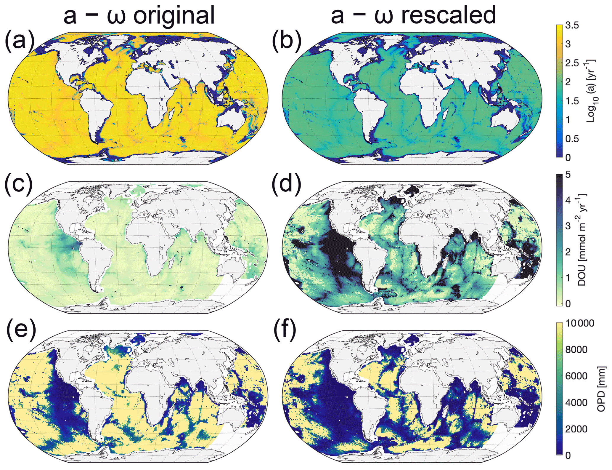
Figure 5 (a) RCM parameter a as a function of sedimentation rate, ω, according to Eq. (13), log₁₀(a)=3.35–14.81⋅ω and (b) and using the same relationship with the resulting parameter linearly rescaled to fall within the range a= [1–100] years. (c, d) Global map of simulated DOU for the parameterizations shown in panels (a) and (b). Positive fluxes are directed into the sediments. (e, f) Global map of simulated OPD for the parameterizations shown in panels (a) and (b). Yellow areas indicate that oxygen flows across the bottom of the model domain (i.e. 10 m). White indicates areas where surface sediment OM contents are not available, i.e. most coastal margins and the south-west Pacific (see Seiter et al., 2005). We omit these grid cells in our simulation.

The mismatch between model results and observations has several reasons. First, it can be partly explained by a bias in the observational data set towards shallower OPD, i.e. exemplified by the upper limit of 1000 mm in the observed OPD, a likely artefact of the data selected, since oxygen is known to penetrate several metres (Glud, 2008) or even down to 60 m (see D'Hondt et al., 2015; Røy et al., 2012), in the oligotrophic gyres of the South Pacific. Indeed, based on observations from the South Pacific gyres, D'Hondt et al. (2015) derive an empirical relationship between OPD, ω and sediment thickness to show that O₂ may be present throughout the entire sediment sequence in 15 %–44 % of the Pacific and 9 %–37 % of the global seafloor. These estimates are further supported by the absence of a sulfate–methane transition zone in these areas (Egger et al., 2018, and see also Fig. 3 for global maps thereof in LaRowe et al., 2020b). The observational OPD data set does not include OPDs of several metres to kilometres that have been observed in the central parts of the oceans (see D'Hondt et al., 2015; Murray and Grunmandis, 1980; Røy et al., 2012).

Furthermore, two simplifications/limitations in the model configuration and in the boundary conditions: first, the applied OM concentration at the SWI (see Seiter et al., 2004) is actually more representative of the mean OM concentration in the upper 5 cm of the sediment. It thus represents a lower limit for the actual SWI concentration. Second, the applied a–ω parameterization used to calculate the average lifetime of the more reactive OM compounds represents only a weak relationship (r²=0.46), as it is only based on a limited number of observations (see Fig. 15b in Arndt et al., 2013). The resulting a values following the parameterization are in the range of 34–2239 years with a mean value of 1240 years (σ=955 years) and are thus likely more representative of an OM mixture of lower reactivity. Both limitations result in lower OM degradation rates and thus an overestimation of the OPD. This realization motivates an additional global simulation of DOU and OPD with a rescaled a–ω relationship (see Fig. 5b, d, f) that yields lower a values, while still following the widely observed inverse trend between a and ω (e.g. Middelburg, 1989; Boudreau and Ruddick, 1991).

The simulated DOUs and OPDs using the rescaled a–ω relationship (Fig. 5d,f) show similar global patterns compared to the original relationship. However, the new model does not generally overpredict the OPDs anymore but is in better agreement with observations. Nevertheless, other model simplifications (i.e. very simplified secondary redox reactions) and caveats in the boundary conditions (i.e. global maps of SWI OM concentrations and sediment accumulation rates), but also the distribution of OM compounds being more complex in reality and site-specific peculiarities are not represented in our approach. Therefore, some degree of mismatch is always to be expected.

Finally, the reoxidation of reduced products can make up a substantial fraction of the oxygen consumption in marine sediments. These secondary reactions consume products originating from anaerobic mineralization (Aller, 1990; Boudreau and Canfield, 1993) and can make up to 56 % (Jørgensen and Kasten, 2006) of the total oxygen consumption in certain environments; thus cannot be ignored. We take these processes into account by running the full version of OMEN-SED-RCM.

3.4 Depth of the sulfate–methane transition zone (SMTZ)

3.4.1 Methodology

Sulfate is the most important terminal electron acceptor in marine sediments on a global scale (Jørgensen, 1982; Thullner et al., 2009). Its depth profile is a macroscopic manifestation of long-term OM degradation in the deeper anoxic sediment and thus crucial for understanding benthic biogeochemical dynamics. Sulfate depth profiles typically show a down core decrease where the gradient is primarily controlled by OM degradation rates and thus both the amount and quality of OM in the deeper sediment. The sediment depth at which downward-diffusing sulfate is completely consumed is referred to as the sulfate–methane transition zone (SMTZ). It separates the sulfate reduction from the methanogenic zone. The SMTZ is a very dynamic redox boundary and its position is very sensitive to changes in environmental conditions (Regnier et al., 2011; Meister et al., 2013). Here, we use OMEN-SED-RCM to simulate changes in the position of the SMTZ in response to a range of sedimentation rates and OM reactivity parameters and compare the simulated patterns with previously observed/simulated patterns (Regnier et al., 2011; Meister et al., 2013).

To this end, we set up a one-dimensional OMEN-SED-RCM simulation that is representative of a shallow depositional environment with a high OM input and a high sedimentation rate. OM concentration is set to 1.1 wt %. We assume bottom water concentrations of ${\mathrm{SO}}_{\mathrm{4}}^{\mathrm{2}-}=\mathrm{28}$ and CH₄=0 mM at the SWI. The model domain is set to 45 m and thus accounts for the active part of the anoxic sediment layer. We use this OMEN-SED-RCM setup to explore the response of the SMTZ to variations in sedimentation rates and apparent OM reactivity (i.e. parameter a). An overview of the applied boundary conditions and parameters is given in Table 3. Because we do not consider active methane venting or upward fluid flow, the location of the SMTZ is mainly controlled by OM degradation.

Table 3 Model boundary conditions representative of shallow shelf marine sediments for the SMTZ simulations. Calculation for ω are from Burwicz et al. (2011).

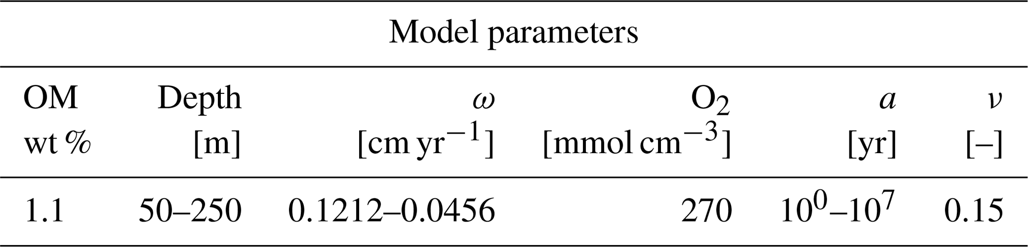
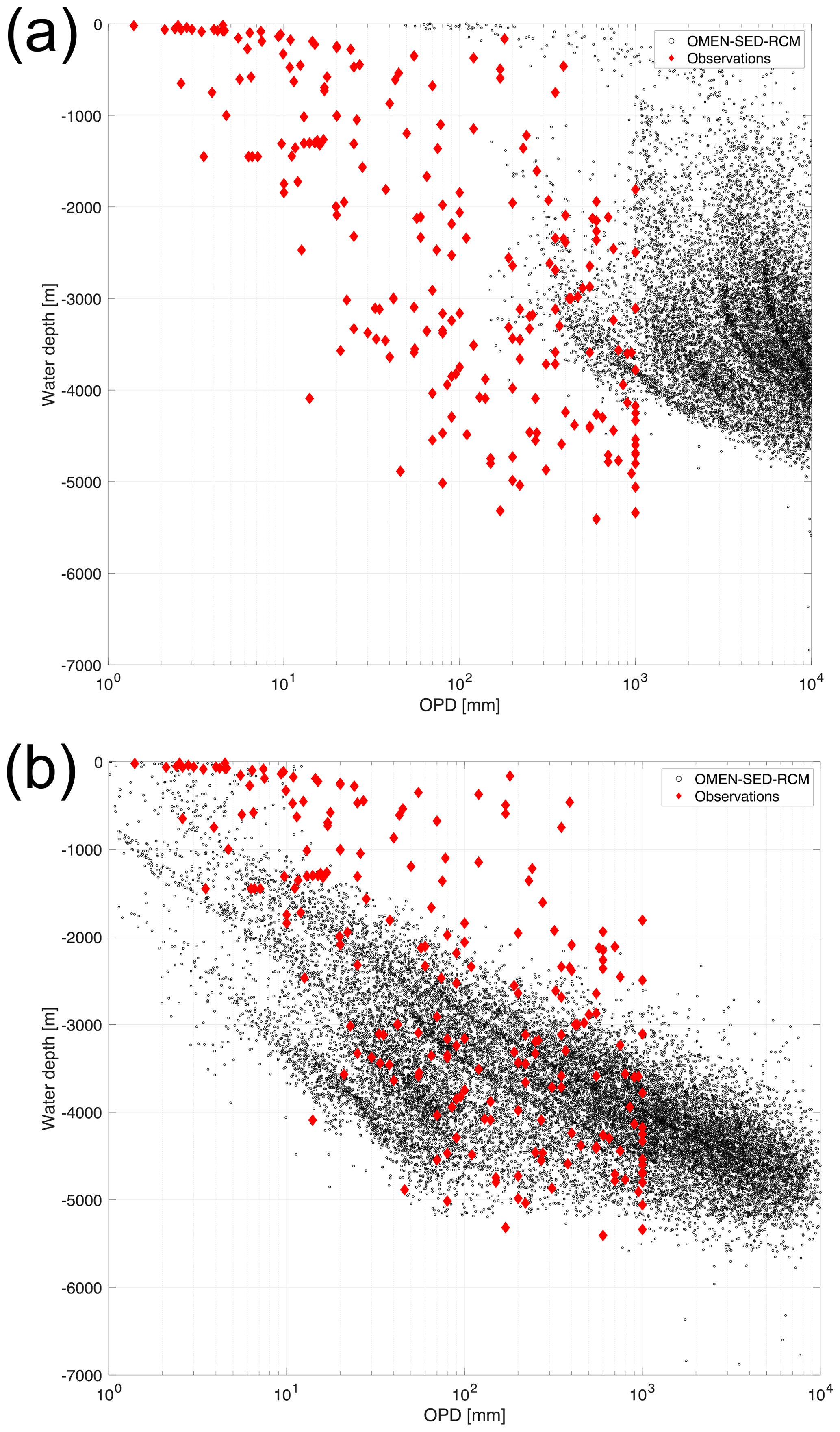
Figure 6 Water depth versus OPD for (a) the original a–ω relationship (Eq. 13) and (b) the rescaled a–ω relationship. OMEN-SED-RCM results are shown as black circles. Observations (shown as red diamonds) are taken from Jahnke et al. (1989), Canfield et al. (1993), Glud et al. (1994), Glud et al. (1998), Glud et al. (1999), Glud et al. (2003), Glud et al. (2009), Wenzhöfer et al. (2001a), Wenzhöfer et al. (2001b), Black et al. (2001), Giordani et al. (2002), Wenzhöfer and Glud (2002), Lansard et al. (2008), Lansard et al. (2009), Sachs et al. (2009), Witte et al. (2003a), Witte et al. (2003b) and Egger et al. (2018).

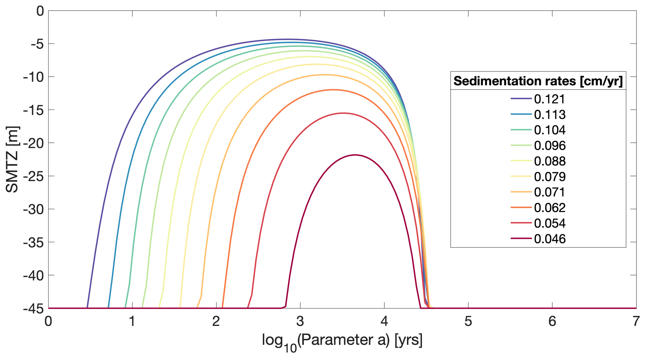
Figure 7 Depth of the SMTZ as a function of OM reactivity parameters and sedimentation rates (ω). For log₁₀(a)<2.9 years and log₁₀(a)>4.5 years, ${\mathrm{SO}}_{\mathrm{4}}^{\mathrm{2}-}$ always reaches the bottom of the model domain. OM is 1 wt %; ν=0.15.

3.4.2 Results

In agreement with results of Regnier et al. (2011) and Meister et al. (2013), OMEN-SED-RCM simulation results show that the sedimentation rate, ω, and parameter a exert a dominant control on the location of the SMTZ (Fig. 7). OMEN-SED-RCM captures the observed/simulated response of the SMTZ to changing environmental conditions well and results are similar to those found in Regnier et al. (2011) and Meister et al. (2013). More specifically, in agreement with previous results, OMEN-SED-RCM shows that very high apparent OM reactivities generally lead to a deep SMTZ. A decrease in apparent OM reactivity (i.e. increase in parameter a) then leads to an upward migration of the SMTZ, until it reaches a minimum depths around intermediate OM reactivity. Hereafter, a further decrease in apparent OM reactivity triggers a new down core migration of the SMTZ. This somewhat counterintuitive behaviour can be explained by a limitation of sulfate reduction rates in the area of both high and low OM reactivities. If apparent OM reactivity is high, a significant fraction of the OM will be degraded in the shallow sediment layer, thus reducing the supply of reactive OM to the sulfate reduction zone. As a consequence, sulfate reduction rates and thus ${\mathrm{SO}}_{\mathrm{4}}^{\mathrm{2}-}$ consumption become limited by a lack of degradable substrate. On the other hand, if apparent OM reactivity is low, sulfate reduction rates become limited by OM reactivity. Both scenarios result in a deep SMTZ. At intermediate OM reactivities, both the quantity and the quality of the OM that is buried into deeper sediment layers are sufficiently high to support enhanced sulfate reduction rates, thus shifting the SMTZ upwards. OMEN-SED-RCM results show that the location of the SMTZ is substrate limited for values below log (a)= [1–3] years (depending on sedimentation rates) and becomes reactivity limited above approximately log (a)= [4.4–4.5] years.

Simulation results also show that OM reactivity exerts the dominant control on the depth of the SMTZ. Changes in sedimentation rate and OM deposition shift (not shown here) but do not change the general pattern. Increasing the deposition flux of OM at the SWI would lead merely to the shallowing of the SMTZ on both ends of the a parameter spectrum (not shown here). Increasing sedimentation rates generally result in shallower SMTZ in the area of high OM reactivities because they increase the flux of OM to the deeper sediment layers. For the same reason, high sedimentation rates also decrease the minimum depth of the SMTZ for intermediate reactivities. The shallowest SMTZ (−5 m) is simulated for the highest ω value and a=10^2.7 years, while the deepest at −20 m occurs when ω is lowest and a=10^3.6 years. In the area of low reactivities (i.e. high parameter a), sedimentation rates, on the other hand, only exert a limited effect on the location of the SMTZ because higher sedimentation rates merely result in a slight increase in OM reactivity at depth.

4 Conclusions

Here we present OMEN-SED-RCM, an extension of the original analytical diagenetic model OMEN-SED (Hülse et al., 2018). OMEN-SED-RCM replaces the simple 2G OM degradation model of the original version with a pseudo-RCM representation of OM degradation. Because the analytical solutions of the coupled transport–reaction equations that underlie OMEN-SED require an exponential form of the OM degradation term, the RCM is approximated by a multi-G approximation, applied here with 500 fractions (Boudreau and Ruddick, 1991; Dale et al., 2015). The RCM and its multi-G approximation (i.e. reaction rate constants and initial fraction of each OM class) are fully constrained by the two free RCM parameters a and ν that control the initial distribution of OM compounds over the reactivity spectrum.

We show that the new version of OMEN-SED is not only able to reproduce observed pore water profiles across a wide range of depositional environments and capture observed global patterns of TEA-fluxes, oxygen penetration depths and biogeochemical reaction rates but also accounts for the widely observed continuous decrease in OM reactivity with sediment depths/burial time and thus provides a more realistic description of anaerobic degradation pathways. This added functionality offers an alternative to the common but simpler 2G model description implemented in the original model, extending the model's applicability to a wider range of environments and timescales, while requiring fewer parameters to describe a wider spectrum of OM reactivity. These improvements were implemented while maintaining the computational advantages of the original version.

Appendix A: Reaction network

Table A1 Primary pathways of organic matter degradation, secondary redox reactions and stoichiometries implemented in the reaction network.

Appendix B: Model transport parameters

(Middelburg et al., 1997)(Boudreau, 1998; Teal et al., 2010)(Middelburg et al., 1997)(Li and Gregory, 1974; Schulz, 2006; Gypens et al., 2008)

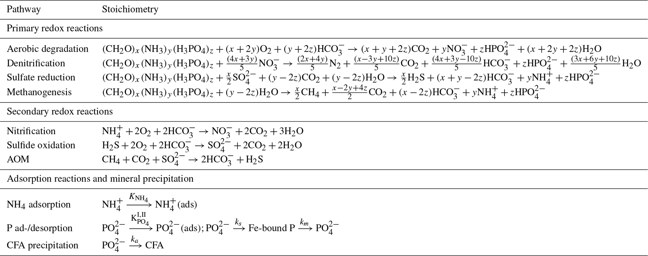
Table B1 Sediment characteristics and transport parameters.

Note: DIC and ALK coefficients are the values of ${\mathrm{HCO}}_{\mathrm{3}}^{-}$ from Schulz (2006).

Appendix C: Biogeochemical model parameters

(Wang and Van Cappellen, 1996; Slomp et al., 1998)(Slomp et al., 1996)

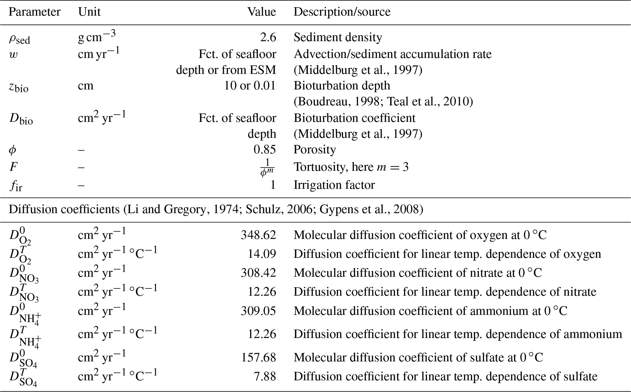
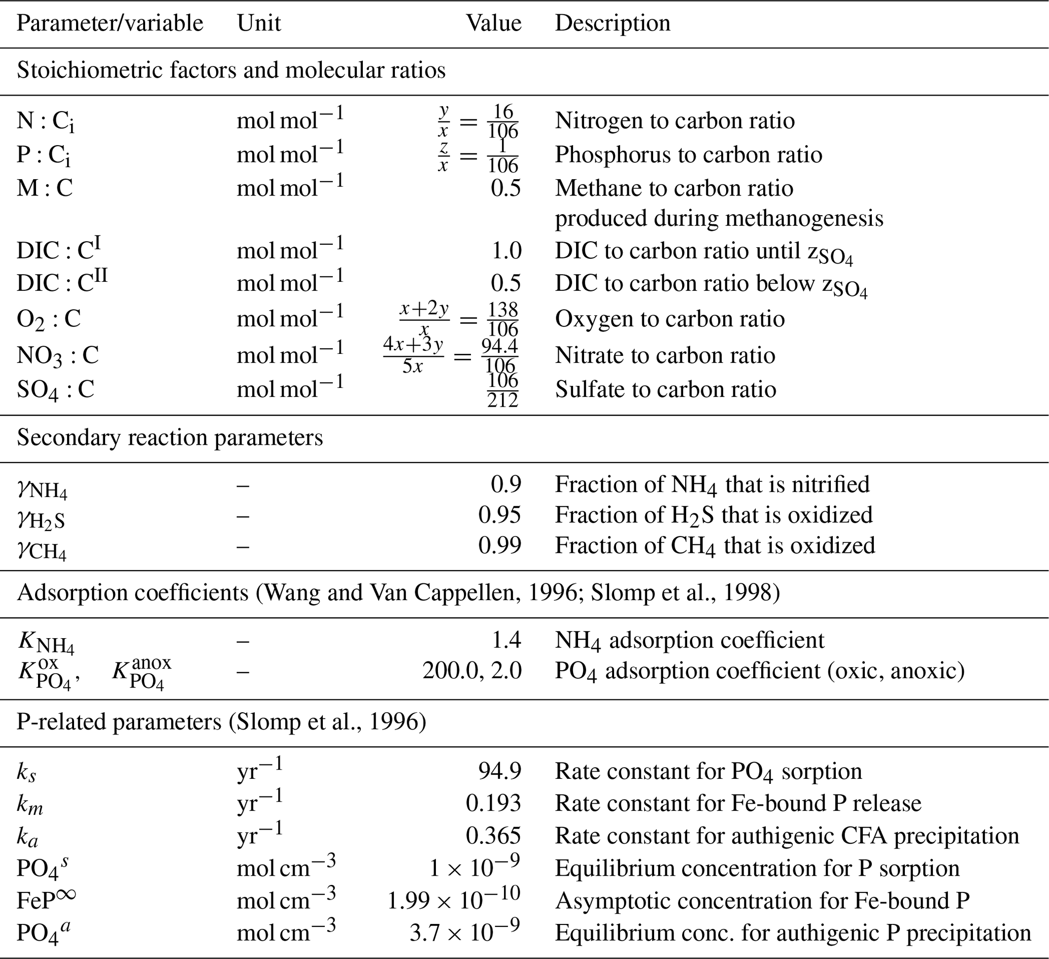
Table C1 Values for biogeochemical parameters used in OMEN-SED-RCM. The variables x, y and z denote the elemental ratio of carbon, nitrogen and phosphorus of the degrading OM (here set to $\mathrm{C}:\mathrm{N}:\mathrm{P}=\mathrm{106}:\mathrm{16}:\mathrm{1}$).