the Creative Commons Attribution 4.0 License.
the Creative Commons Attribution 4.0 License.
 | 22 Nov 2021
B-flood 1.0: an open-source Saint-Venant model for flash-flood simulation using adaptive refinement
Geoffroy Kirstetter
Olivier Delestre
Pierre-Yves Lagrée
Stéphane Popinet
Christophe Josserand
The French Riviera is very often threatened by flash floods. These hydro-meteorological events, which are fast and violent, have catastrophic consequences on life and property. The development of forecasting tools may help to limit the impacts of these extreme events. Our purpose here is to demonstrate the possibility of using b-flood (a subset of the Basilisk library http://basilisk.fr/, last access: 8 November 2021), which is a 2D tool based on the shallow-water equations and adaptive mesh refinement. The code is first validated using analytical test cases describing different flow regimes. It is then applied to the Toce river valley physical model produced by ENEL-HYDRO in the framework of the CADAM project and on a flash-flood case over the urbanized Toce area produced during the IMPACT project. Finally, b-flood is applied to the flash flood of October 2015 in Cannes in south-eastern France, which demonstrates the feasibility of using software based on the shallow-water equations and mesh refinement for flash-flood simulation in small watersheds (less than 100 km2) and on a predictive computational timescale.
- Article
(10482 KB) - Full-text XML
- BibTeX
- EndNote


The south of France is very often affected by flash floods, strong and rapid events that arise particularly in the summer and autumn due to slow-moving convective storms bringing moisture from the Mediterranean Sea, with the induced rainfall amplified by topographic influences (Sene, 2012). Some big and catastrophic flash floods occurred in September 2002 in the Gard region (Delrieu et al., 2005), in June 2010 around Draguignan city (Javelle et al., 2014), and more recently in October 2015 in the French Riviera (Carrega, 2016; Saint-Martin et al., 2018), particularly affecting the city of Cannes. Watersheds located in the French Riviera are steep and generally cover less than 100 km2, which induces short hydrological responses (from a few minutes to a few hours). On these watersheds, two types of flood can be defined (World Meteorological Organization, 2011): riverine flood, which is encountered in the upstream part of the river basin, and urban flood, which occurs in the downstream part of the watershed. Most of these watersheds are densely urbanized, and this density is increasing over time (Fox et al., 2019), and thus people's lives, property (Carrega, 2016; Saint-Martin et al., 2018), and even health (Jacq et al., 2016) are highly threatened by these hazardous climatic events. The simulation of such disastrous climatic events therefore appears to be a key and crucial objective for everything from public safety to urban planning but also because of its important economic consequences. In particular, shorter-than-real-time simulations allowing for practical predictions of the storm location and the subsequent flood propagation represent a major challenge for the numerics. In this context of real-time forecasting, there are three main categories of flood-mapping methodologies for the upstream part. The first methodology consists of using the 2D shallow-water equations or simplifications (kinematic wave, diffusive wave, and local inertia approximations) and/or a parallelized (CPU or GPU) resolution algorithm to speed up calculation times (Lisflood, Iber, Telemac, etc.). This was first applied for mapping large rivers at a continental scale and at fairly high resolutions (Pappenberger et al., 2012; Alfieri et al., 2014; Sampson et al., 2015; Dottori et al., 2016). These methods are gradually evolving towards more local applications and finer resolutions (metres) in order to map floods on small rivers (Cea and Bladé, 2015; Xia et al., 2017; García-Feal et al., 2018; Nguyen et al., 2016; Neal et al., 2018; Sanders and Schubert, 2019). The second flood-mapping methodology is based on the application of 1D hydrodynamic models. It is based on the extraction of cross sections from a digital terrain model (DTM) (Choi and Mantilla, 2015; Le Bihan et al., 2017; Lamichhane and Sharma, 2018). The third methodology consists of a direct infilling of the DTM from a locally determined water level. This group includes the AutoRoute method (Follum et al., 2017), as well as several approaches based on the concept of height above the nearest drainage point (height above nearest drainage, HAND) (Rennó et al., 2008; Nobre et al., 2011), including f2HAND (Speckhann et al., 2018), Geoflood (Zheng et al., 2018), and MHYST (Rebolho et al., 2018). With this approach, a flow–height relationship is determined from the geometry of the cross section extracted from the DTM (averaged over a section for HAND-based approaches) using a hydraulic formula (Manning Strickler, Debord, etc.). These approaches have the advantage of being very efficient in computing time (Teng et al., 2017), although their accuracy limits have already been highlighted compared to conventional 2D approaches (Afshari et al., 2018). Recently, Hocini et al. (2021) proposed a comparison of mapping methods from each of these families in the context of flash floods observed in south-eastern France. This work has shown that the 2D method was more accurate. Moreover, most of the operational flood forecasting systems are based on a coupling of a rainfall-runoff–hydrological model and a routing–hydraulic model, as reviewed in Jain et al. (2018). Concerning the downstream part of the domain, which is densely urbanized (Saint-Martin et al., 2018; Fox et al., 2019), because of the complex geometry of the city it is recommended to use 2D modelling (Mignot et al., 2019). For these reasons, we have chosen to use a fully integrated model based on the 2D shallow-water equations with rain source terms solved thanks to a finite-volume scheme on an adaptive mesh using the software Basilisk (http://basilisk.fr/, last access: 8 November 2021). The originality of the model is in gathering, using the same code, both the fluvial and urban flood configurations using up-to-date numerical schemes with a forecasting computation time (Buttinger-Kreuzhuber et al., 2019; Horváth et al., 2020) thanks to the automatic adaptive mesh refinement.
In Sect. 2 we present the model, the numerical method, and the adaptive mesh technique. In Sect. 3 we first exhibit the ability of the Basilisk software to catch different types of flow regimes for analytical solutions developed in MacDonald et al. (1997) and implemented in the SWASHES library (Delestre et al., 2013). We then apply Basilisk for the Toce river valley physical model (Valiani et al., 1999) produced by the ENEL-HYDRO (formerly ENEL CRIS) laboratories in Milan in the framework of the CADAM project (Concerted Action on Dam break Modelling; Morris, 2000). This is a 1 : 100 scale physical model of a submersion wave in part of the Toce river valley in the occidental Alps, Italy. The irregularities in the domain give birth to coexistence of subcritical flow with supercritical flow. This allows the verification of Basilisk as being able to properly catch the dynamics of the riverine flood encountered in the upper part of the watershed. Basilisk is then used on the urbanized Toce produced in the framework of project IMPACT (Testa et al., 2007). It shows its ability to correctly reproduce the dynamics of urban flood met in the downstream part of the watershed. This model represents a urban district where buildings are modelled using concrete blocks placed in the upstream part of the Toce river model. Finally, b-flood is applied to the flash flood of 3 October 2015 in Cannes in south-eastern France.
Floods have horizontal length scales much larger than the vertical one. This observation is used as an hypothesis for the model. This gives a pressure that is hydrostatic as a first approximation. Integrating the Navier–Stokes equations over the thin flow depth then gives the following classical Saint-Venant equations (de Saint-Venant, 1871):
where h is the local flow depth, qx and qy are the two components of the horizontal depth-averaged flow rate, zb is the topography, Sh is the mass source term responsible for rainfall and infiltration, and Sx and Sy are the two components of the friction terms for the topography. See De Vita et al. (2020) for a discussion of the loss of detail in the transverse integration and Popinet (2020) for non-hydrostatic corrections.
The shallow-water equations (Eqs. 1, 2, and 3) can be written in conservative vector form as
where is the vector of the conserved variables, and are the flux, Szb is the gravity source term, and S is used for the other source terms. This system of equations is solved thanks to a finite-volume approach on a square grid.
2.1 Time step and time advance algorithm
We use a predictor–corrector scheme as the time-stepping algorithm: it is second-order in time, and the source terms are dealt with using a time-split method; see Sect. 2.3 below. We can then re-write the Eq. (4) without the source terms as follows:
where f(U) is a numerical flux. Thus, the two steps of the predictor–corrector algorithm can be written for the time step n+1 as follows:
where the superscript is devoted to the time step. We note the velocity field . We use the Courant–Friedrichs–Lewy (CFL) stability criteria (Courant et al., 1928) to define the maximal stable time step as follows:
where a is the magnitude of the velocity of waves and xmin is the minimal size on the grid.
2.2 Flux calculation and well-balanced gravity source term on abrupt topography
To compute the numerical flux F(Un) between two cells, we use the HLLC (Harten–Lax–van Leer contact) solver of Toro (2019) and the Toro et al. (1994) solver as an approximate Riemann solver, which uses a MUSCL-type reconstruction in space with a generalized minmod limiter where θ=1.3 (e.g. Van Leer, 1979). This solver conserves the positivity of the water depth and the equilibrium states known as “lake-at-rest” states thanks to the hydrostatic reconstruction of Audusse et al. (2004). Delestre et al. (2012) have shown that this scheme can non-physically prevent water from flowing when the topography is very steep and the water layer is thin. This situation is far from being trivial since it inevitably occurs as soon as it rains. This is why we add the new second-order reconstruction introduced by Buttinger-Kreuzhuber et al. (2019); Horváth et al. (2020) and derived from Chen and Noelle (2017), which makes it possible to remedy this problem.
2.3 Additional source terms
We treat all the other source terms with the time-splitting technique. If we call S the sum of all source terms other than gravity, then the final line of the time scheme (Eq. 7) can be written as follows:
We will describe in the following paragraphs the different terms that can be modelled in this source term S.
2.3.1 Rain
The rain is simply treated as Srain=R, where R is the local intensity of the rain (in m s−1). This source term is added in the mass equation (Eq. 1) and was validated in a previous study using Basilisk (Kirstetter et al., 2016). Note that it is possible to integrate rain from Météo-France RADAR PANTHERE data directly in the code thanks to the read_lamedeau() function (see METEO-FRANCE, 2021).
2.3.2 Infiltration
We have integrated the infiltration source term of the Green–Ampt model (e.g. Green and Ampt, 1911). This model allows us to consider infiltration depending on the hydraulic conductivity K, the free space in the porosity material Δθ, the wetting front capillary pressure ψ, and the volume infiltrated V.
This source term is also added in the mass equation (Eq. 1).
2.3.3 Friction
Two different friction models are implemented, using the Manning or Darcy–Weisbach relations. These terms are explicitly written as follows:
where nm is the coefficient of Manning, f is the coefficient of Darcy, and g is the acceleration of gravity.
As recommended in a previous study (Delestre et al., 2009), we treat the friction term in a semi-implicit way. This leads to the modification of the velocity field obtained from . The velocity along x is changed as follows for Manning's law:
and as follows for Darcy–Weisbach's law:
The same transformation is applied on the y component of the velocity field.
2.3.4 Velocity threshold
When it rains on a very steep topography, waterfalls can occur. In this case, the physics describing the phenomenon is very different from the laws of turbulent friction that we use. It can therefore appear in the simulations that speeds that are too high and do not correspond to any physical reality. This is why we have developed a simple velocity transformation that prevents the norm of the vector velocity field from exceeding a certain threshold value set by the user. It is written as follows:
where T is the threshold value. The same transformation is applied on the y component of the velocity field. A scalar field is associated with this function that allows us to see where this modification has been realized during the simulation. We can thus verify that it concerns very small areas of the simulation where the slope is almost vertical.
2.4 Adaptive mesh refinement (AMR)
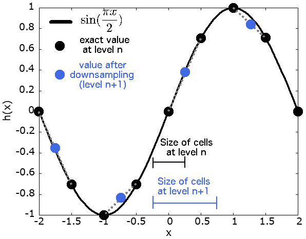
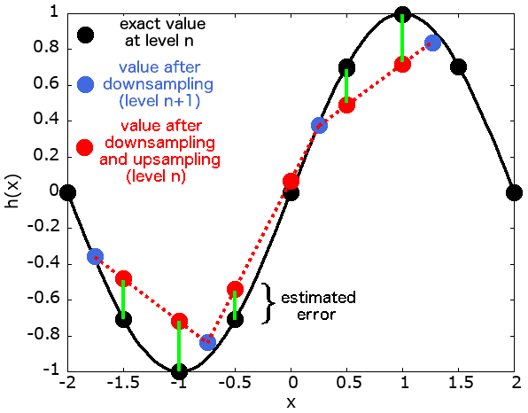
The b-flood software takes advantage (in addition to other techniques) of the adaptive mesh refinement (AMR) technique developed on Basilisk by S.Popinet (Popinet, 2015). This process is very well explained in van Hooft et al. (2018) and in the sandbox of Van Hooft on the Basilisk website (van Hooft, 2021). We recall here the general mechanism, drawing heavily on the previously cited publications. The adapt_wavelet() function allows us to refine or to enlarge the mesh according to the error estimated by the algorithm between two levels of refinement on one or more scalar or vector fields. The error criterion and the fields concerned are set by the user. If the error estimated is greater than the user-defined criterion, the algorithm will refine the cell into four smaller daughter cells. If the error estimate is less than two-thirds of the same criterion, then the algorithm considers the resolution to ne too fine and that the computing time should thus be increased. The function will therefore combine the four cells concerned into a single large cell. If the error is between two-thirds of the criterion and a whole criterion, then nothing happens. The criterion can finally be seen as the maximum permissible error between two levels of refinement. The process of the evaluation of the error on the example of a perfect sinusoidal swell is described in Figs. 1 and 2. It is important to note that the function used to calculate the new field value after refining or “coarsening” the cells is usually a linear interpolation, but it can be set differently by the user for each field. For example, the function used to refine the topography is not a linear interpolation, but simply the value that the topography had before coarsening. The practical use of this function is detailed in the three examples of real cases published below. In addition to the adaptive refinement process, it is possible to refine certain parts of the mesh statically using the refine() and coarsen() functions.
2.5 B-flood: a subset of Basilisk
In practice, the b-flood software is a sub-component of the open-source Basilisk software created by Popinet (2013). This means that it takes advantage of all the features of Basilisk: it is completely free and open-source software. In addition to the AMR described above, it also allows parallel computing. Experienced users will be able to develop their own modules, while casual users will be able to copy and paste the sample scripts given in the rest of this article. It is still recommended to learn how to use the basics of Basilisk before using b-flood, which is made easier thanks to the various tutorials available on the website (http://basilisk.fr/).
3.1 Analytical test cases
It is important to ensure that the numerical schemes we use are consistent. We test them on complete benchmarks, i.e. the transition from subcritical flow, when the wave velocity is higher than the flow velocity to supercritical flow, as well as the transition from supercritical to subcritical flow, which is characterized by the presence of a shock. The following test cases can be found in the software SWASHES published in Delestre et al. (2013). They are designed to test the validity of implementation of source terms and the consistency of the numerical scheme by comparing the numerical solution with the analytical one.
3.1.1 Subcritical to supercritical flow with Manning friction
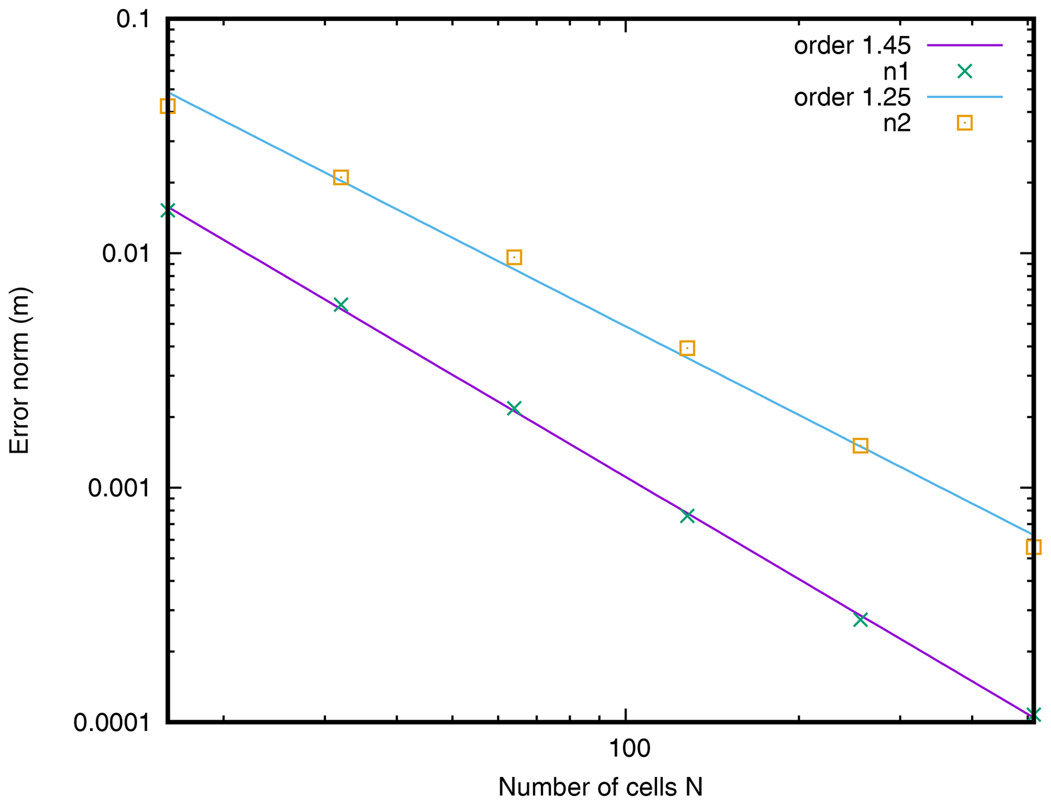
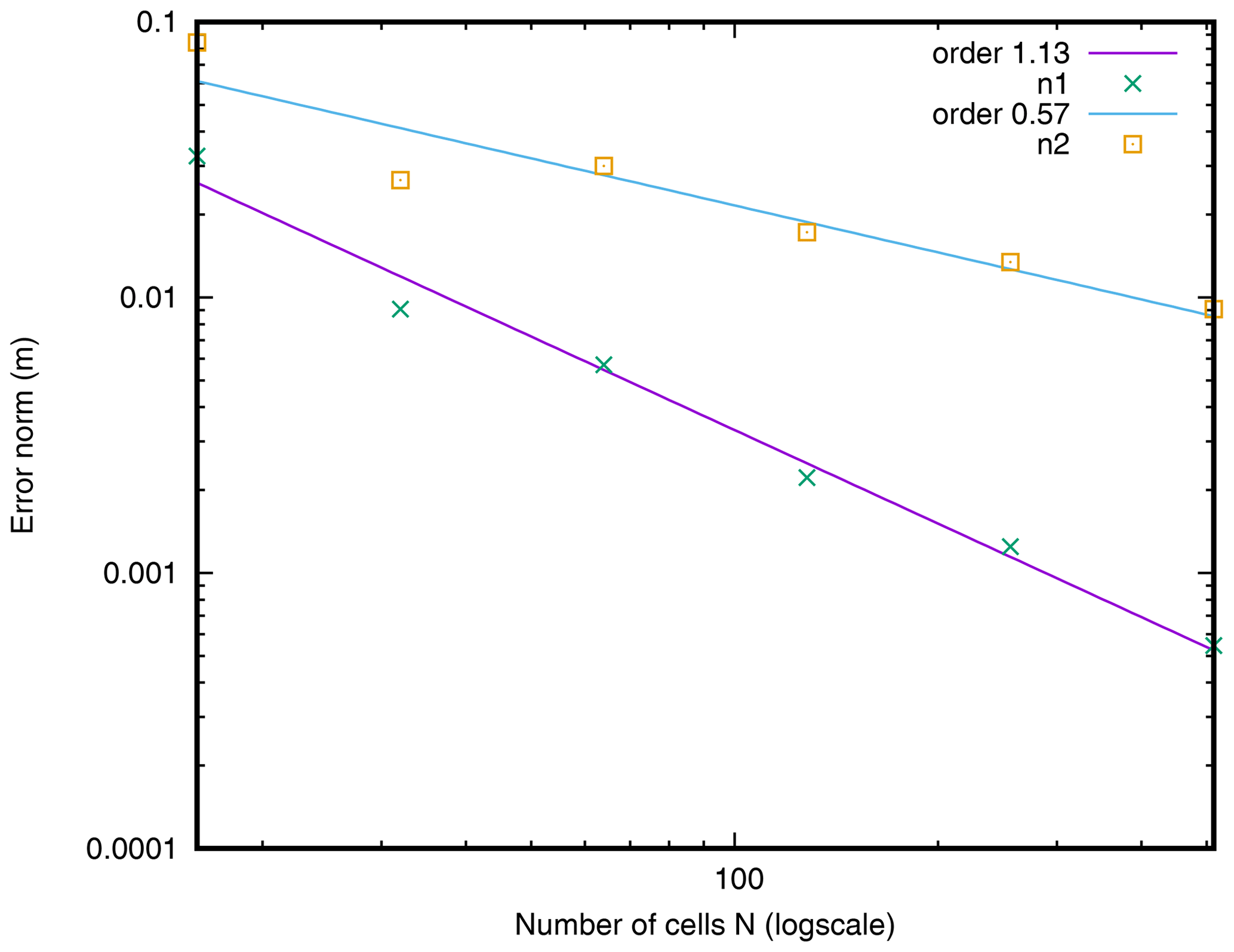
In this benchmark, we test the transition from a subcritical to a supercritical regime with Manning's law of friction. A constant flow q0=2 m2 s−1 is imposed on the left boundary of the flume on the topography plotted in Fig. 3. The case is in 1D and the domain is 1000 m long and initially dry. The friction is modelled by the Manning law with n=0.0218 m s. The flow is subcritical for the coordinate x<500 m and supercritical otherwise. The duration of the experiment is 2000s. We checked that the flow is stationary at the end of the run. At the end of the experiment, we compute the following error norms:
with N the total number of cells, hi the water depth computed on b-flood at the cell i, hei the exact solution for the water depth at the location of the cell i, and Σi the operator to sum over all the cells.
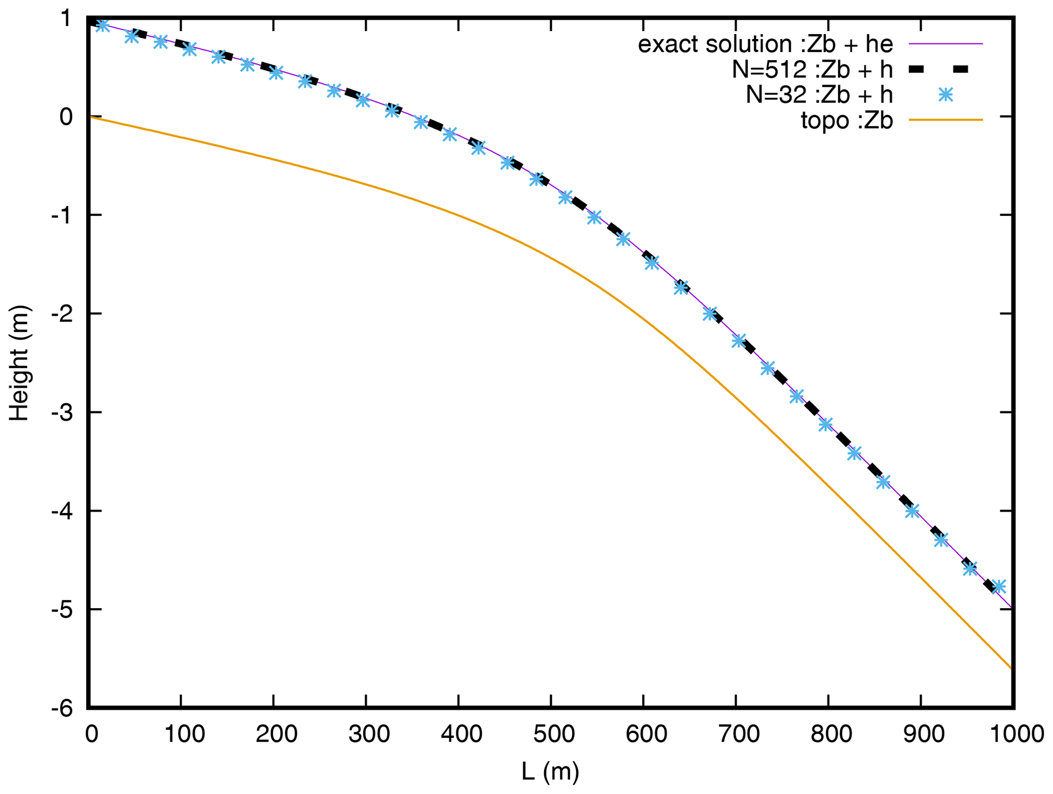
Figure 3Comparison of the water height profiles between the simulation with the analytical solution of the Manning friction test case for two different resolutions.
The water heights profile at resolutions N=32 and N=512 are compared to the exact solution in Fig. 3. The convergence of the different error norms according to the resolution is shown in Fig. 4 in log scale for both resolution axes. As we can see, the simulated profile converges toward the analytical profile, and all the error norms converge to zero with an order larger than 1.
3.1.2 Transonic transition and shock with Darcy–Weisbach friction
In this benchmark, we validate the transition from a supercritical flow to a subcritical flow, which is characterized by the presence of a shock. The domain is 100 m long and a constant discharge of q0=2 m2 s−1 is imposed on the left boundary (upstream) on the topography plotted in Fig. 5. At the right boundary (downstream), the water height is fixed to its analytical value. The flow is subcritical at the left of the slope, becomes supercritical via a sonic point, and then becomes subcritical again via a shock. The case is in 1D and the friction is modelled by the Darcy–Weisbach law with a coefficient f=0.093. The duration of the experiment is 200 s. We checked that the flow is stationary at the end of the run.
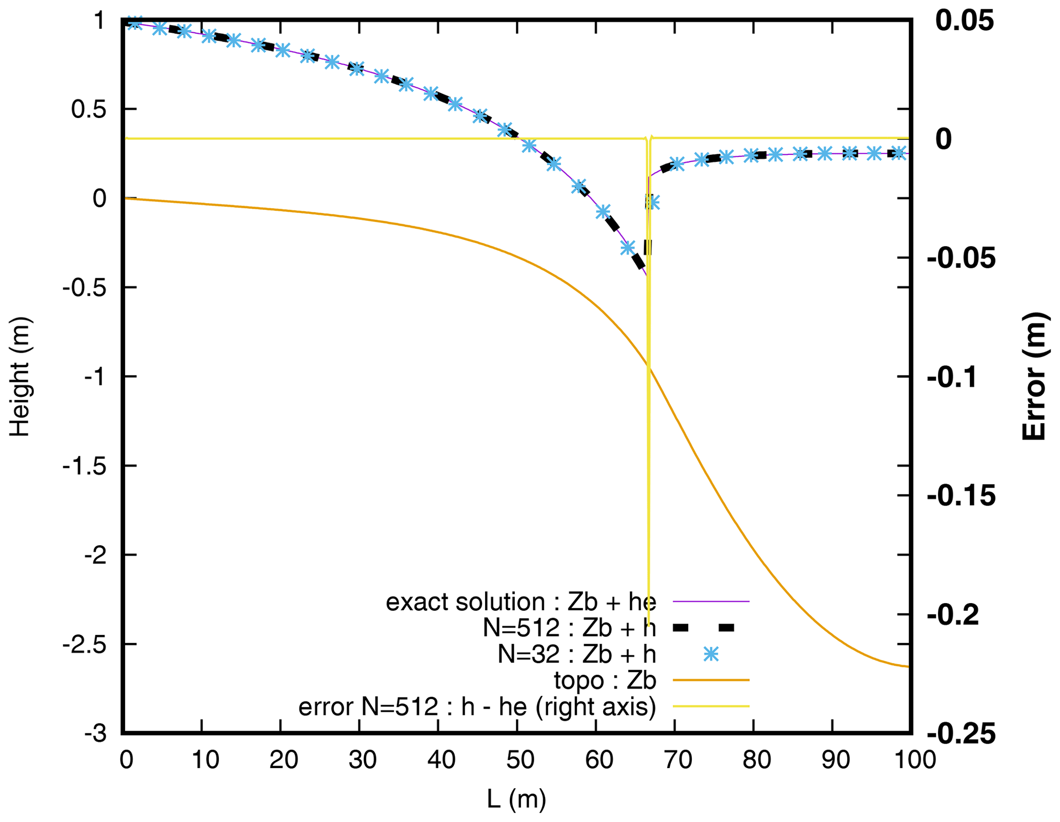
Figure 5Comparison between the simulation with the analytical solution of the transonic test case for two different resolutions.
As done before, the water depth profile at resolutions N=32 and N=512 are compared to the exact solution in Fig. 5. In the same figure, we represent the distribution of the error: h−he as a function of the position. We can see that a large error is found at the shock location. This is due to the fact that the position of the shock is necessarily approached at the resolution step dx . The convergence of the different error norms according to the resolution can be seen in Fig. 6. The presence of the error on the location of the shock necessarily induces orders of convergence smaller than in the previous case, but sufficiently convincing for the convergence of the code.
3.2 B-flood versus experimentation: “the Toce model”
In order to validate b-flood, we use a flood experiment recreated by researchers: the Toce Valley model. The Toce model was designed to study the capabilities of different numerical models to accurately represent flow characteristics. This model was done for the CADAM project by Soares Frazao and Testa (1999). It is a reproduction of the Toce river valley in Italy at a 1 : 100 scale. It is fully instrumented with many stations that measure water level profiles at multiple locations. A nozzle is placed at the entrance of the domain to deliver a controlled flow rate.
3.2.1 Fluvial case
The first case is done on the entire river which is 50 m long and 11 m large. The DTM is at a resolution of 5 cm, note that this includes the reproduction of houses. The topography with the position of the 21 gauge stations can be seen in Fig. 7, where the downward direction is from left to right. The missing numbers (P6, P7, P11, P12, P14–17, P20, and P22) are gauges that did not work during the experiment and therefore were not provided by the experimenters. The imposed inlet condition is an hydrograph. The hydrograph is composed of a brutal rising stage from 0 to 210 L s−1 and a slower and continuous descent phase that reaches up to 60 L s−1 at the end of the experiment, as we can see in Fig. 8. The duration of the experiment is 180 s.

Figure 7Topography of the fluvial case with the position and name of the gauge stations. The inflow is coming from the left border of the domain.
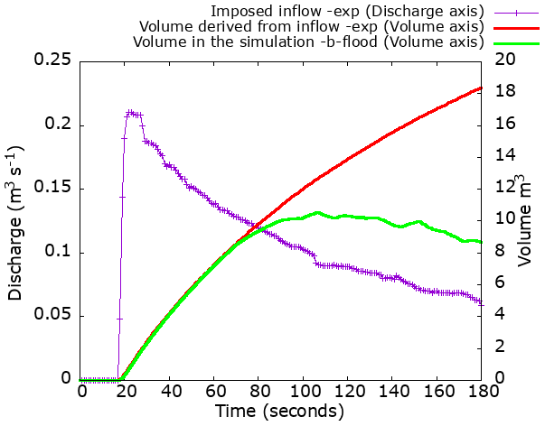
Figure 8Hydrograph of the imposed inflow on the left boundary. Comparison of the volume of water in the simulation and the experimental one.
We reproduce the exact same case with b-flood with a minimal cell size of cm and a maximal size of cm. We model the friction with Manning's law, and we set Manning's coefficient to n=0.0162 m s as recommended by the CADAM report. On the left edge we impose a water elevation on the edge as an inlet condition such that the flow is the same as that imposed by the hydrograph. The boundary condition on the normal velocity is a Neumann condition () and on the tangential velocity it is a Dirichlet condition (Uy=0). We make sure that we impose the right flow rate by comparing the volume in the b-flood simulation with the imposed flow rate, converted to volume using the following equation: . We can see in Fig. 8 that the correct inflow is imposed in the simulation. Note that the volume in the simulation “stalls” from the imposed volume around t=80 s, when the water flow exits the simulation domain at the right edge. On the right edge of the domain, we set a condition of free exit of water and flow. For adaptive refinement, the error threshold is set at 5 mm on the water level field. To ensure the exact reproduction of the experimental case, some precautions must be taken. We artificially set a small time step Δt=0.01 s at time t=17 s to make sure we capture the short rise of the hydrograph. Still with the aim of capturing the rise of the hydrograph, we leave off the adaptive refinement until time t=18 s. Note that we do this because the simulation domain is empty for the first 17 s, which will not happen in a real case where rivers are flowing and rain is falling. The simulation runs for 18 966 s on an Apple laptop equipped with a 2.8 GHz Intel Core i5 dual-core processor. We measure the water depth profiles at the exact positions of the 22 gauge stations, and we record movies of the flow characteristics during the experiment: water depth, velocity of flow, and Froude number. All the movies are available on the b-flood website, as are other data and the entire code. We can see the flood wave front propagation and the resulting automatic adaptive refinement in Fig. 9.
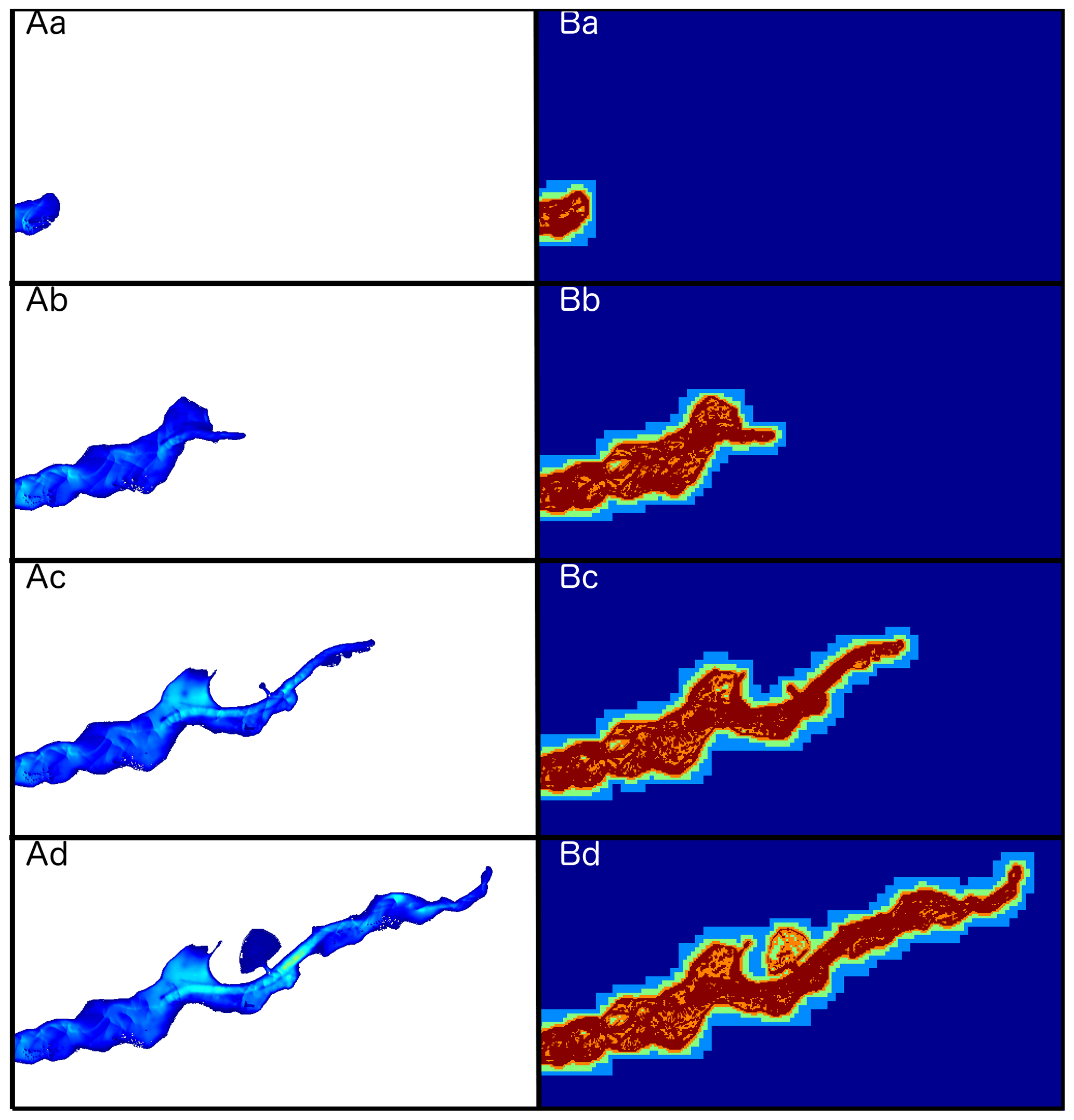
Figure 9Picture of the water depth (A) and the refinement level (B) at t=21 s (a), t=35 s (b), t=49 s (c)m and t=63 s (d). The minimum value for the water height (A) is 1 cm, corresponding to the dark blue colour, and the maximum is 40 cm, corresponding to the light blue colour. For the refinement level (B), the minimum value is a cell of 68 cm × 68 cm, corresponding to dark blue, and the maximum value is a cell of 4.2 cm × 4.2 cm, corresponding to red.
To quantify the performance of b-flood, we define the following different numbers, starting with e1 (metres) and e1r (no unit):
where tend is the final time of the experiment, hexp is the experimental value of the water depth at the considered water gauge, and hnum is the value of the water depth found by b-flood at the same location. The time ts is defined as the time when both numerical and experimental values of the water depth exceed the threshold value of 5 mm. Note that e1 and e1r are positive if hnum is mostly greater than hexp and vice versa. e1r is equal to e1 normalized by the mean height of the experimental case. e1r should be read as the mean percentage difference with respect to the experimental height.
We also define e2 and e2r as follows:
Note that unlike e1 and e1r, e2 and e2r are always positive. As e1r, e2r is equal to e2 normalized by the mean value of hexp. In addition, both e1r and e2r should be read as the mean percentage of the root-mean-square error (RMSE) with respect to the experimental height.
Finally, we define the arrival time delay as the time between the two instants when at least 5 mm of water arrives at the measuring station in the real case and in the case simulated by b-flood. This arrival time delay is a good metric to quantify the capacity of b-flood to mimic the dynamics of the experimental case. Note that a positive arrival time delay corresponds to the case where water arrives first in the numerical case: arrival time delay is positive when b-flood is early and negative when b-flood is late.
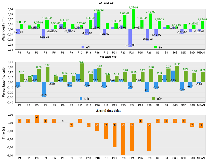
We report the values of the different norms in Fig. 10. We can see that the mean value of the RMSE (e2) at all the stations is around 16 cm and is around 20 % for the root mean square of the relative error (e2r). We report the water depth measured at stations P24, P10, and P2 in Fig. 11. Measuring station 24 has the worst RMSE and one of the worst arrival time delays. We can see that although it slightly underestimates the water level, b-flood does capture the dynamics of the flood wave on this station. Station 10 is the worst in terms of relative error. However, we can see that b-flood models the flow with a sufficient precision at this station as well. On the other hand, b-flood provides a very good estimate of the flow at station 2.

In conclusion, we can say that b-flood correctly models this fluvial case of flood on impermeable soil with imposed inflow and the presence of houses.
3.2.2 Urban case
The second case of validation is reproducing “the Model city flooding experiment benchmark” presented in Alcrudo et al. (2003) and Testa et al. (2007) (data are freely available from https://doi.org/10.1080/00221686.2007.9521831). This model is built on the first 15 m of the precedent Toce model. The authors added 20 buildings distributed in four aligned rows, and nine gauge stations are distributed around the buildings and at the entrance of the flow. The topography of the case and the locations of gauge stations are shown in Fig. 12. The imposed entry condition is again a hydrograph. The flow rate goes from 0 to a maximum of 130 L s−1 in 4 s and then progressively decreases to 30 L s−1 in 50 s, as we can see in Fig. 13. This condition in fact reproduces the typical water flow of a flash flood. The experiment lasts 60 s.
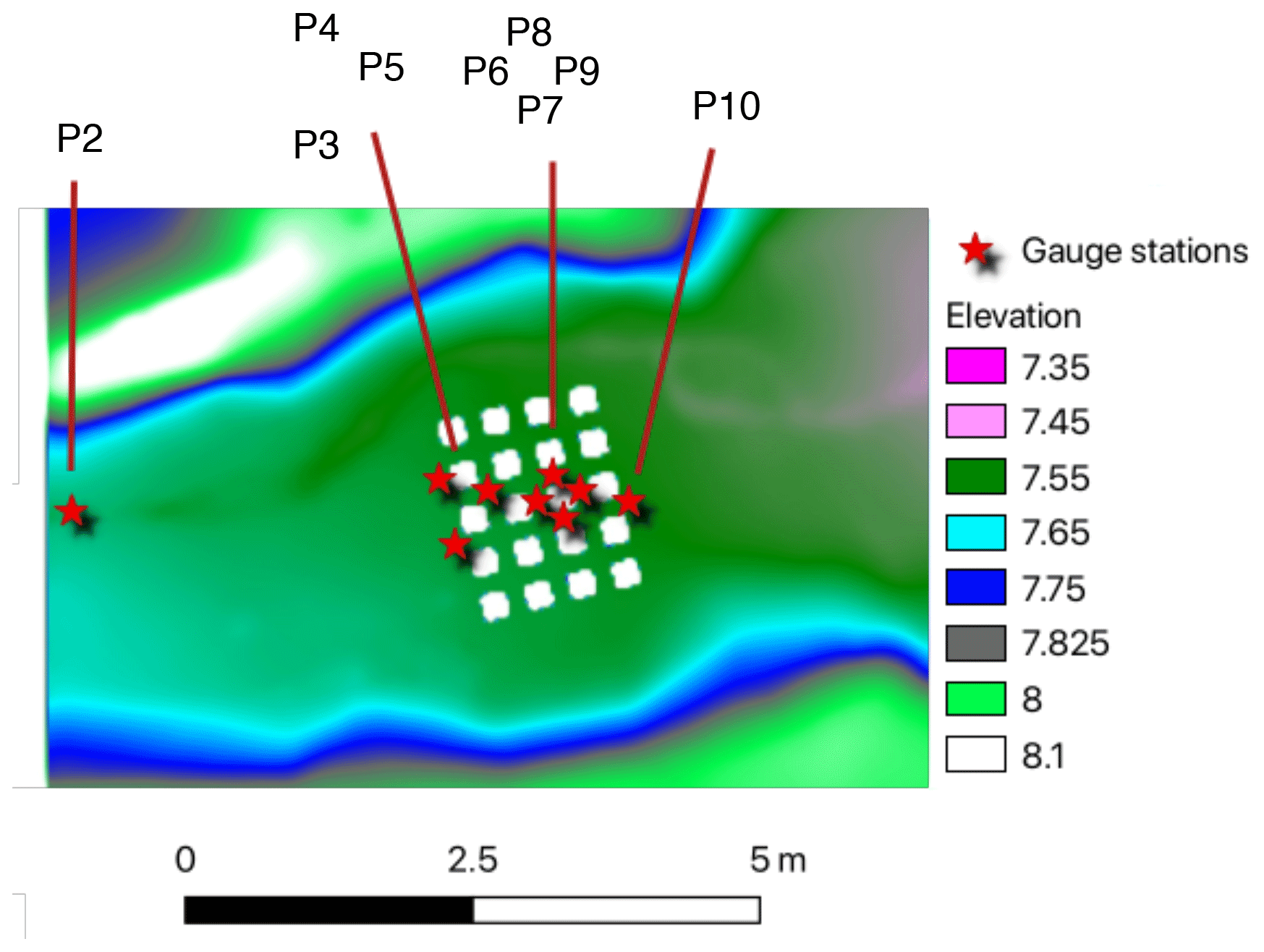
Figure 12Zoom on the first 10 m of the topography of the urban model with positions of buildings and gauge stations.
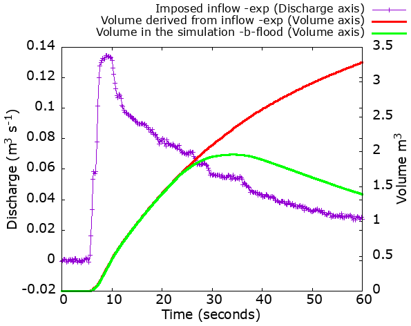
Figure 13Hydrograph of the imposed inflow on the left boundary. Comparison of the volume of water in the simulation and the experimental one.
We reproduce this case using b-flood. The domain consists of cells of sizes between cm and cm. For adaptive refinement, the error threshold is set at 1 mm on the water level field. We set as an entry condition on the left boundary a constant water height such that the inflow is the one imposed by the hydrograph. The boundary condition on the normal velocity is a Neumann condition () and a Dirichlet condition (Uy=0) on the tangential velocity. Exactly as done previously for the case validated for the “fluvial Toce”, we compare the volume of water entering the simulation and the volume of water entering the experiment (thanks to the hydrograph) in Fig. 13, and a perfect match is obtained. We use Manning's friction law with the value n=0.0162 m s, as recommended by Alcrudo et al. (2003). To replicate the vertical walls of the houses, we raise the topography of our simulation by an immense height at the site. This has the effect of producing near-vertical walls (see Sect. 2.2). The simulation runs for 23 047 s on an Apple laptop equipped with a 2.8 GHz Intel Core i5 dual-core processor. We can see the arrival of the flood wave simulated by b-flood as well as the adaptive refinement in Fig. 14. In this figure, we can see that the front of the flood wave is refined to the maximum but that the refinement becomes coarse again once the wave has passed if the water flow is not too complex.
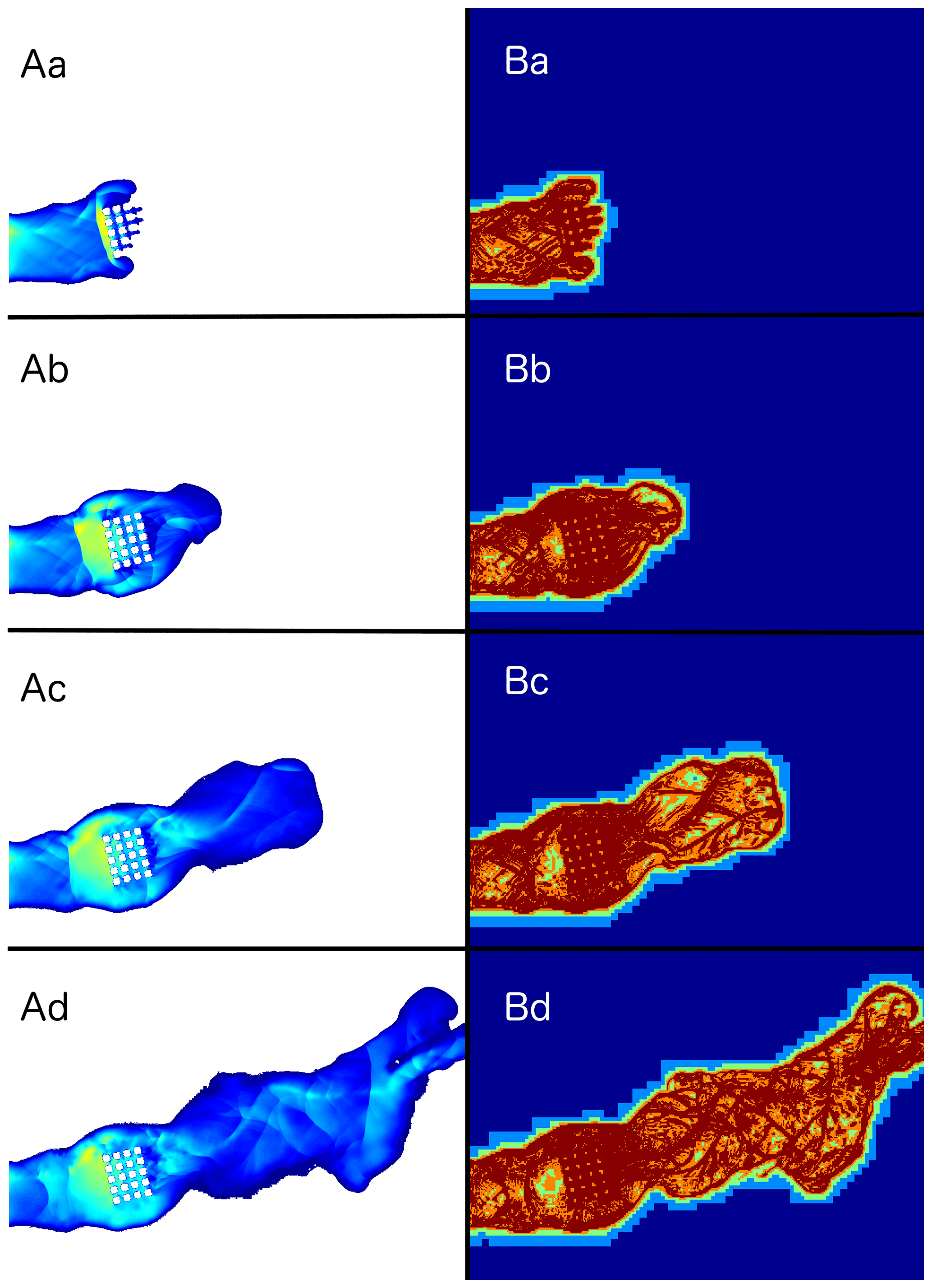
Figure 14Picture of the water depth (A) and the refinement level (B) at t=10 s (a), t=13 s (b), t=17 s (c), and t=26 s (d). The minimum value for the water height (A) is 1 cm, corresponding to the dark blue colour, and the maximum is 20 cm, corresponding to the light blue colour. For the refinement level (B), the minimum value is a cell of 23 cm × 23 cm, corresponding to the dark blue, and the maximum value is a cell of 1.5 cm × 1.5 cm, corresponding to red.
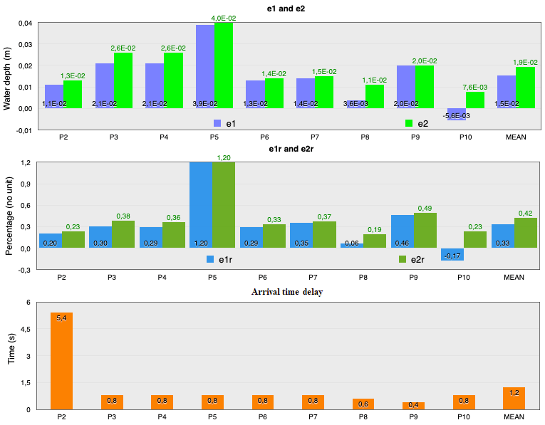
We record in the simulation the water heights at the exact locations where the measurement stations are in the experiment. Following this, for each of these stations we calculate the norms e1, e1r, e2, and e2r. We also calculate the delay time between the arrival of the flood wave in the numerical case and in the experimental case. These results are shown in Fig. 15. We can see that e1 remains more or less the same as in the fluvial case, with a mean value of 1.9 cm. However, the relative value e1r is greater than the previous case, with a mean of 42 %. This value may seem high, but it mainly reflects the error made at station 5. In Fig. 16, the water height recorded at station P5 is shown, which gives the worst result. It should be noted that other studies of this case also give “bad” results at this station and not at the others. As an example, we have given the results of (Kim et al., 2014) that the authors obtained on the exact same case with their Saint-Venant solver on an unstructured grid using triangular elements. This leads us to believe that the error comes from the presence of a hydraulic jump that the Saint-Venant equations do not allow to be predicted correctly, and therefore this error cannot be attributed to the numerical method. The arrival time delay does not exceed 5 s for all the stations and its maximum value is on station P2, which allows us to verify that the dynamics of the arrival of the flood wave is well simulated. We can see in Fig. 16 that the dynamics modelling therefore remains convincing.

The produced results allow us to conclude on the validity of our simulations in this case of urban flooding on impermeable soil.
Here we demonstrate the possibility of using b-flood, a software based on shallow-water equations and mesh refinement, in a real flash-flood situation in a small watershed (less than 100 km2). For this, we simulate the case of the flash flood that took place in Cannes (France) on 3 October 2015 (Carrega, 2016; Saint-Martin et al., 2018). The city of Cannes is located in south-eastern France. On Saturday, 3 October 2015, between 18:00 and 23:00 LT (local time), a large amount of rain fell on the Alpes-Maritimes department in France: in some areas 200 mm of rain was recorded over less than 3 h. This outstanding meteorological event killed 20 people and the CCR (Caisse Centrale de Réassurance, a French public reinsurer; see http://www.ccr.fr, last access: 8 November 2021) estimated the total material lost to be valued between EUR 500 million and EUR 650 million. Around the river Siagne, the SISA (Syndicat Intercommunal de la Siagne et ses Affluents, which aimed to fight against floods in the territory of the member municipalities; today, SISA has been dissolved, and their mission has been taken over by the SMIAGE since 1 January 2018) recorded a rain intensity larger than 200 mm h−1 around 20:30 LT. This kind of meteorological event, where a large amount of rain is localized on a small area during a short period of time, is known as a “flash flood” and in this case led to the appearance of torrents of water throughout the streets of Cannes. Moreover, in the upstream area, the soil was already saturated by a heavy rain that occurred on 2 October, and in the city the storm water system was also saturated.
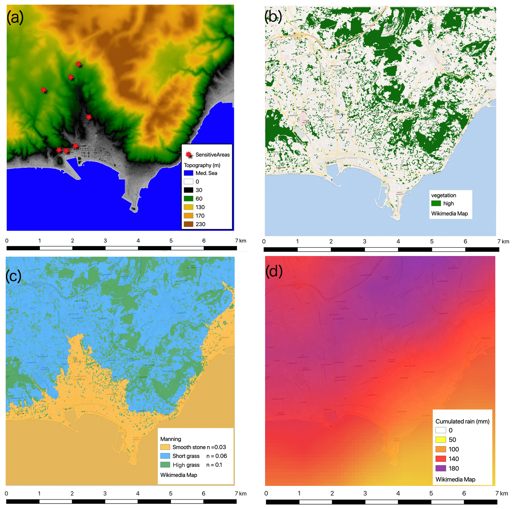
Figure 17(a) Topography of the simulated domain and position of sensitive areas. (b) High-vegetation zone. (c) Manning coefficient values. (d) Accumulated rain during the rain event.
To simulate this event with b-flood, we use a digital terrain model at a resolution of 1 m, courtesy of the IGN (National Institute of Geographic and Forestry Information of France) (RGE-ALTI). We also use the digital surface model (DSM) to add buildings. The buildings are simulated thanks to an elevation of the topography corresponding to their real heights. The total size of the domain is 7 km × 7 km and fully encompasses the catchment area of the city of Cannes. The maximum cell size is m, and the minimum cell size is m. We use adaptive refinement with a threshold value of 5 cm on the height of water. We added an even smaller cell size, Δxspe=6.8 m, to mesh specific sensitive areas more precisely, e.g. town halls, fire stations, hospitals, and police stations. This mesh size allows us to be more accurate in these sensitive areas without slowing down our simulation. The DTM and DSM topography used and the location of these sensitive areas can be seen in Fig. 17a.
We use Manning's law and the infiltration source term. IGN also provides soil plant occupation maps (BD TOPO). We can see the zones of high vegetation in Fig. 17b. We use these areas to set the value of the Manning coefficient and the various infiltration parameters. The Manning coefficient is set to n=0.1 m s in high-vegetation zones, n=0.03 m s where the topography is below 50 m to represent the urban zone, and n=0.06 m s everywhere else; see Fig. 17c. The infiltration parameters are set to loamy-sand values in high-vegetation areas (ψ=6.1 cm, cm h1, θ=5 %) and to values of sandy clay everywhere else (ψ=21 cm, cm h1, θ=5 %).
We use the source term of rain to add the precipitation measured by Météo-France; these are provided free of charge (RADAR PANTHERE). These data are at 5 min time steps, and the pixels are of 1 km × 1 km size. We can see the cumulated rain during the event in Fig. 17d.
We fix the threshold value on the celerity to Vthreshold=10 m s−1 in order to avoid slowing down the code unnecessarily (see Sect. 2.3.4). In fact, when rain is added to a quasi-vertical topography, the speed of the water can reach high values, which (in addition to not representing reality) slow down the code. The duration of the simulated event is 5 h. The simulation was performed on a 16-core desktop for 6472 s, which is consistent with the time delay of rainfall predictions. We record the maximal value of the water depth field during the entire event, as shown in Fig. 18 highlighting the flood extent. Movies of the evolution of the water depth, the celerity, and the level of refinement can be seen online on the website of b-flood (Kirstetter et al., 2019), showing the good qualitative behaviour of b-flood in reproducing the whole event. During the process of writing this article, another article (Kirstetter et al., 2020) was published using b-flood on the flooding of the French Riviera during October 2015. In this paper, the team compared the b-flood results to measurements made in situ and a good quantitative agreement was found.
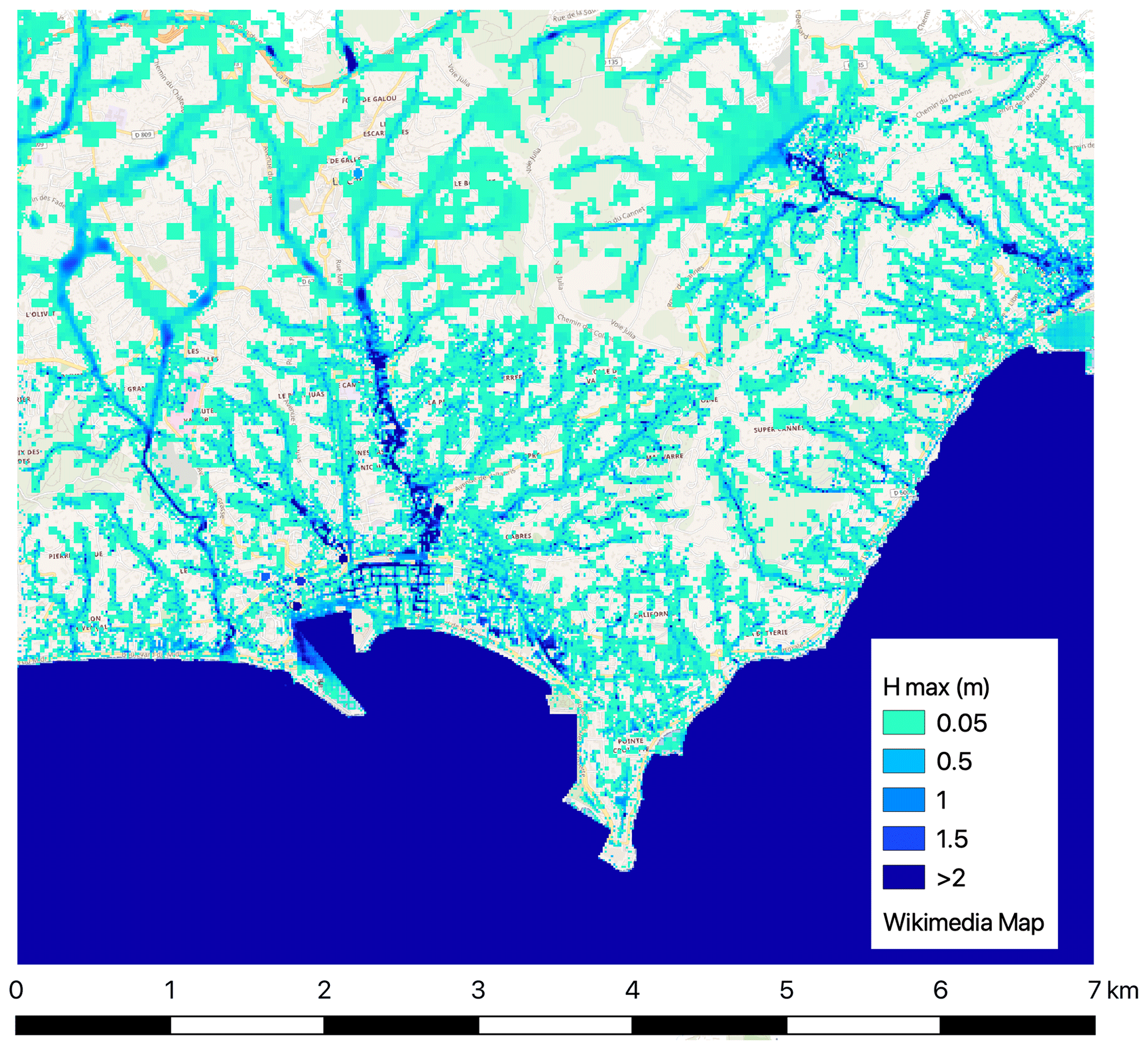
Figure 18Flood extent of the event simulated by b-flood.
This paper presented b-flood, an open-source Saint-Venant model for simulations of surface flows in two dimensions using adaptive refinement. The code is completely free and open source like the Basilisk software from which it is derived. The model uses a well-balanced scheme that does not prevent water from flowing over steep topography.
The validity of the numerical scheme has been tested on two analytical benchmarks. The convergence of the scheme has been observed with a good order of convergence. The code has been then tested on two experimental cases in the Toce Valley, one fluvial and the other urban. The results of the simulation gave satisfactory agreement with the experimental results. Finally, we demonstrated the practical effectiveness of b-flood on a real case of flash flooding on a small watershed in the south of France: the October 2015 flooding of the city of Cannes in the French Riviera. This event caused 20 fatalities and a lot of material damage. The city of Cannes faced 200 mm of precipitation over less than 3 h. In the upstream area, the soil was already saturated by a heavy rain that occurred on 2 October, and in the city the storm water system was also saturated. This has demonstrated the feasibility of using a software based on shallow-water equations and mesh refinement for flash-flood simulation on small watersheds (less than 100 km2). Remarkably, for this practical case predictions of the flood dynamics and localization could be deduced over a computational time compatible with the rainfall predictions, opening the way to real-time flood forecasting.
Future work will focus on (1) implementing hydraulic structures such as culverts, gates, and weirs and (2) coupling this overland flow model with a storm water network model. This will improve b-flood's capability when performing more complete flash-flood simulations, particularly in southern French watersheds.
The address of the relevant Zenodo folder is as follows: https://doi.org/10.5281/zenodo.4617606 (Kirstetter and Popinet, 2021). Note that the Basilisk software needs to be installed before visiting this address: http://www.basilisk.fr/src/INSTALL (last access: 8 November 2021). You will find the (open-source) code and the different data files required to reproduce our results here: http://basilisk.fr/sandbox/b-flood/Readme (Kirstetter et al., 2019). It should be noted that we do not have the right to distribute the DTM file of the IGN's topography of Cannes or the Météo-France files. The case study of Cannes performed in this paper is therefore unfortunately not reproducible.
The movie representing the water height during the Cannes flood (Cannes-height.mpg) and the video representing the refinement level of the cells of the same simulation (Cannes-level.mpg) can be downloaded from the following address: https://doi.org/10.5281/zenodo.5061754 (Kirstetter, 2021).
GK developed the code for b-flood and took care of the technical part. OD took care of the test cases and brought his expertise on the different competing codes of b-flood. PYL supervised the project and brought his expertise on the different physical models. SP developed the codes on which b-flood is based (basilisk) and brought his technical expertise on the technical and algorithmic part. CJ was in charge of the acquisition of the funds and supervised the project. GK prepared the manuscript with contributions from all co-authors.
The authors declare that they have no conflict of interest.
Publisher's note: Copernicus Publications remains neutral with regard to jurisdictional claims in published maps and institutional affiliations.
We would like to thank François Bourgin for the initial idea of this paper. We would like to thank the IGN for providing us with the topographic data and Météo-France for providing us with the data from their RADAR PANTHERE. We also thank the AXA Foundation for Research fund for their financial support at the very beginning of this study.
This paper was edited by Bethanna Jackson and reviewed by two anonymous referees.
Afshari, S., Tavakoly, A. A., Rajib, M. A., Zheng, X., Follum, M. L., Omranian, E., and Fekete, B. M.: Comparison of new generation low-complexity flood inundation mapping tools with a hydrodynamic model, Journal of Hydrology, 556, 539–556, https://doi.org/10.1016/j.jhydrol.2017.11.036, 2018. a
Alcrudo, F., Garcia, P., Brufau, P., Murillo, J., Garcia, D., Mulet, J., Testa, G., and Zuccala, D.: The Model City Flooding Experiment, in: EC Contract EVG1-CT-2001-00037 IMPACT Investigation of Extreme Flood Processes and Uncertainty, Proc. 2nd Project Workshop, 12–13 September 2002, Mo i Rana, Norway, 2003. a, b
Alfieri, L., Salamon, P., Bianchi, A., Neal, J., Bates, P., and Feyen, L.: Advances in pan-European flood hazard mapping, Hydrol. Process., 28, 4067–4077, https://doi.org/10.1002/hyp.9947, 2014. a
Audusse, E., Bouchut, F., Bristeau, M.-O., Klein, R., and Perthame, B. T.: A fast and stable well-balanced scheme with hydrostatic reconstruction for shallow water flows, SIAM J. Sci. Comput., 25, 2050–2065, 2004. a
Buttinger-Kreuzhuber, A., Horváth, Z., Noelle, S., Blöschl, G., and Waser, J.: A fast second-order shallow water scheme on two-dimensional structured grids over abrupt topography, Adv. Water Resour., 127, 89–108, 2019. a, b
Carrega, P.: Les inondations azuréennes du 3 octobre 2015: un lourd bilan lié à un risque composite – The Côte d'Azur floods on 3 october 2015: heavy consequences linked to a composite risk, Pollution Atmosphérique, 228, 1–26, https://doi.org/10.4267/pollution-atmospherique.5475, 2016 (in French). a, b, c
Cea, L. and Bladé, E.: A simple and efficient unstructured finite volume scheme for solving the shallow water equations in overland flow applications, Water Resour. Res., 51, 5464–5486, https://doi.org/10.1002/2014WR016547, 2015. a
Chen, G. and Noelle, S.: A new hydrostatic reconstruction scheme based on subcell reconstructions, SIAM J. Numer. Anal., 55, 758–784, 2017. a
Choi, C. C. and Mantilla, R.: Development and Analysis of GIS Tools for the Automatic Implementation of 1D Hydraulic Models Coupled with Distributed Hydrological Models, J. Hydrol. Eng., 20, 06015005, https://doi.org/10.1061/(ASCE)HE.1943-5584.0001202, 2015. a
Courant, R., Friedrichs, K., and Lewy, H.: Uber die partiellen Differenzengleichungen der mathematischen Physik, Math. Ann., 100, 32–74, https://doi.org/10.1007/BF01448839, 1928. a
Delestre, O., Cordier, S., James, F., and Darboux, F.: Simulation of Rain-Water Overland-Flow, in: Proceedings of the 12th international conference on Hyperbolic Problems, 9–13 June 2008, University of Maryland, College Park, USA, 1–11, 2009. a
Delestre, O., Cordier, S., Darboux, F., and James, F.: A limitation of the hydrostatic reconstruction technique for Shallow Water equations, C. R. Math., 350, 677–681, 2012. a
Delestre, O., Lucas, C., Ksinant, P.-A., Darboux, F., Laguerre, C., Vo, T.-N.-T., James, F., and Cordier, S.: SWASHES: a compilation of shallow water analytic solutions for hydraulic and environmental studies, Int. J. Numer. Meth. Fl., 72, 269–300, 2013. a, b
Delrieu, G., Ducrocq, V., Gaume, E., Nicol, J., Payrastre, O., Yates, E., Kirstetter, P.-E., Andrieu, H., Ayral, P.-A., Bouvier, C., Creutin, J.-D., Livet, M., Anquetin, S., Lang, M., Neppel, L., Obled, C., Parent-Du-Châtelet, J., Saulnier, G.-M., Walpersdorf, A., and Wobrock, W.: The catastrophic flash-flood event of 8–9 September 2002 in the Gard Region, France: a first case study for the Cévennes–Vivarais Mediterranean Hydrometeorological Observatory, J. Hydrometeorol., 6, 34–52, 2005. a
de Saint-Venant, A. B.: Théorie du mouvement non permanent des eaux, avec application aux crues des rivières et à l'introduction des marées dans leurs lit, Comptes Rendus des séances de l'Académie des Sciences, 73, 237–240, 1871 (in French). a
De Vita, F., Lagrée, P.-Y., Chibbaro, S., and Popinet, S.: Beyond Shallow Water: Appraisal of a numerical approach to hydraulic jumps based upon the Boundary Layer theory, Eur. J. Mech. B – Fluid., 79, 233–246, https://doi.org/10.1016/j.euromechflu.2019.09.010, 2020. a
Dottori, F., Salamon, P., Bianchi, A., Alfieri, L., Hirpa, F. A., and Feyen, L.: Development and evaluation of a framework for global flood hazard mapping, Adv. Water Resour., 94, 87–102, https://doi.org/10.1016/j.advwatres.2016.05.002, 2016. a
Follum, M. L., Tavakoly, A. A., Niemann, J. D., and Snow, A. D.: AutoRAPID: A Model for Prompt Streamflow Estimation and Flood Inundation Mapping over Regional to Continental Extents, J. Am. Water Resour. As., 53, 280–299, https://doi.org/10.1111/1752-1688.12476, 2017. a
Fox, D. M., Youssaf, Z., Adnès, C., and Delestre, O.: Relating imperviousness to building growth and developed area in order to model the impact of peri-urbanization on runoff in a Mediterranean catchment (1964–2014), Journal of Land Use Science, 14, 210–224, https://doi.org/10.1080/1747423X.2019.1681528, 2019. a, b
García-Feal, O., González-Cao, J., Gómez-Gesteira, M., Cea, L., Domínguez, J. M., and Formella, A.: An Accelerated Tool for Flood Modelling Based on Iber, Water, 10, 10, https://doi.org/10.3390/w10101459, 2018. a
Green, W. H. and Ampt, G.: Studies on Soil Phyics, J. Agr. Sci., 4, 1–24, 1911. a
Hocini, N., Payrastre, O., Bourgin, F., Gaume, E., Davy, P., Lague, D., Poinsignon, L., and Pons, F.: Performance of automated methods for flash flood inundation mapping: a comparison of a digital terrain model (DTM) filling and two hydrodynamic methods, Hydrol. Earth Syst. Sci., 25, 2979–2995, https://doi.org/10.5194/hess-25-2979-2021, 2021. a
Horváth, Z., Buttinger-Kreuzhuber, A., Konev, A., Cornel, D., Komma, J., Blschl, G., Noelle, S., and Waser, J.: Comparison of Fast Shallow-Water Schemes on Real-World Floods, J. Hydraul. Eng., 146, 05019005, https://doi.org/10.1061/(ASCE)HY.1943-7900.0001657, 2020. a, b
Jacq, L., Vallet-Anfosso, A., Tibi, T., Genillier, P., Petit, B., Desse, D., Franke, F., Bellemain-Appaix, A., Rafidiniaina, D., and Bernasconi, F.: Événements cardiovasculaires lors des intempéries exceptionnelles du 3 octobre 2015 touchant la Côte d’Azur, xXIIe Congrès du Collège national des cardiologues des hôpitaux, 17–18 November 2016, Annales de Cardiologie et d'Angéiologie, 65, 373–374, https://doi.org/10.1016/j.ancard.2016.06.002, 2016 (in French). a
Jain, S. K., Mani, P., Jain, S. K., Prakash, P., Singh, V. P., Tullos, D., Kumar, S., Agarwal, S. P., and Dimri, A. P.: A Brief review of flood forecasting techniques and their applications, International Journal of River Basin Management, 16, 329–344, https://doi.org/10.1080/15715124.2017.1411920, 2018. a
Javelle, P., Demargne, J., Defrance, D., Pansu, J., and Arnaud, P.: Evaluating flash-flood warnings at ungauged locations using post-event surveys: a case study with the AIGA warning system, Hydrolog. Sci. J., 59, 1390–1402, https://doi.org/10.1080/02626667.2014.923970, 2014. a
Kim, B., Sanders, B. F., Schubert, J. E., and Famiglietti, J. S.: Mesh type tradeoffs in 2D hydrodynamic modeling of flooding with a Godunov-based flow solver, Adv. Water Resour., 68, 42–61, 2014. a
Kirstetter, G.: Water height and level of refinement during the flood of Cannes, Zenodo [video], https://doi.org/10.5281/zenodo.5061754, 2021. a
Kirstetter, G. and Popinet, S.: B-flood 1.0: an open-source Saint-Venant model for flash flood simulation using adaptive refinement (Version 1), Zenodo [code], https://doi.org/10.5281/zenodo.4617606, 2021. a
Kirstetter, G., Hu, J., Delestre, O., Darboux, F., Lagrée, P.-Y., Popinet, S., Fullana, J.-M., and Josserand, C.: Modeling rain-driven overland flow: Empirical versus analytical friction terms in the shallow water approximation, J. Hydrol., 536, 1–9, 2016. a
Kirstetter, G., Delestre, O., Lagrée, P.-Y., Popinet, S., and Josserand, C.: b-flood, sandbox of Basilisk.fr [code], available at: http://basilisk.fr/sandbox/b-flood/Readme, last access: 26 June 2019. a, b
Kirstetter, G., Bourgin, F., Brigode, P., and Delestre, O.: Real-Time Inundation Mapping with a 2D Hydraulic Modelling Tool Based on Adaptive Grid Refinement: The Case of the October 2015 French Riviera Flood, in: Advances in Hydroinformatics, Springer, Singapore, 335–346, 2020. a
Lamichhane, N. and Sharma, S.: Effect of input data in hydraulic modeling for flood warning systems, Hydrolog. Sci. J., 63, 938–956, https://doi.org/10.1080/02626667.2018.1464166, 2018. a
Le Bihan, G., Payrastre, O., Gaume, E., Moncoulon, D., and Pons, F.: The challenge of forecasting impacts of flash floods: test of a simplified hydraulic approach and validation based on insurance claim data, Hydrol. Earth Syst. Sci., 21, 5911–5928, https://doi.org/10.5194/hess-21-5911-2017, 2017. a
MacDonald, I., Baines, M., Nichols, N., and Samuels, P.: Analytic benchmark solutions for open-channel flows, J. Hydraul. Eng., 123, 1041–1045, 1997. a
METEO-FRANCE: Cumul Lame D'Eau Radar, Panthere Météo-France, available at: https://donneespubliques.meteofrance.fr/?fond=produit&id_produit=103&id_rubrique=34, last access: 8 November 2021. a
Mignot, E., Li, X., and Dewals, B.: Experimental modelling of urban flooding: A review, J. Hydrol., 568, 334–342, https://doi.org/10.1016/j.jhydrol.2018.11.001, 2019. a
Morris, M. W.: CADAM Concerted Action on Dambreak Modelling, Final Report February 1998–January 2000, Tech. Rep. Report SR 571, EC Contract number ENV4-CT97-0555, 2000. a
Neal, J., Dunne, T., Sampson, C., Smith, A., and Bates, P.: Optimisation of the two-dimensional hydraulic model LISFOOD-FP for CPU architecture, Environ. Model. Softw., 107, 148–157, https://doi.org/10.1016/j.envsoft.2018.05.011, 2018. a
Nguyen, P., Thorstensen, A., Sorooshian, S., Hsu, K., AghaKouchak, A., Sanders, B., Koren, V., Cui, Z., and Smith, M.: A high resolution coupled hydrologic–hydraulic model (HiResFlood-UCI) for flash flood modeling, J. Hydrol., 541, 401–420, https://doi.org/10.1016/j.jhydrol.2015.10.047, 2016. a
Nobre, A., Cuartas, L., Hodnett, M., Rennó, C., Rodrigues, G., Silveira, A., Waterloo, M., and Saleska, S.: Height Above the Nearest Drainage – a hydrologically relevant new terrain model, J. Hydrol., 404, 13–29, https://doi.org/10.1016/j.jhydrol.2011.03.051, 2011. a
Pappenberger, F., Dutra, E., Wetterhall, F., and Cloke, H. L.: Deriving global flood hazard maps of fluvial floods through a physical model cascade, Hydrol. Earth Syst. Sci., 16, 4143–4156, https://doi.org/10.5194/hess-16-4143-2012, 2012. a
Popinet, S.: Basilisk, available at http://basilisk.fr (last access: 8 November 2021), 2013. a
Popinet, S.: A quadtree-adaptive multigrid solver for the Serre–Green–Naghdi equations, J. Comput. Phys., 302, 336–358, 2015. a
Popinet, S.: A vertically-Lagrangian, non-hydrostatic, multilayer model for multiscale free-surface flows, J. Comput. Phys., 418, 109609, https://doi.org/10.1016/j.jcp.2020.109609, 2020. a
Rebolho, C., Andréassian, V., and Le Moine, N.: Inundation mapping based on reach-scale effective geometry, Hydrol. Earth Syst. Sci., 22, 5967–5985, https://doi.org/10.5194/hess-22-5967-2018, 2018. a
Rennó, C. D., Nobre, A. D., Cuartas, L. A., ao Vianei Soares, J., Hodnett, M. G., Tomasella, J., and Waterloo, M. J.: HAND, a new terrain descriptor using SRTM-DEM: Mapping terra-firme rainforest environments in Amazonia, Remote Sens. Environ., 112, 3469–3481, https://doi.org/10.1016/j.rse.2008.03.018, 2008. a
Saint-Martin, C., Javelle, P., and Vinet, F.: DamaGIS: a multisource geodatabase for collection of flood-related damage data, Earth Syst. Sci. Data, 10, 1019–1029, https://doi.org/10.5194/essd-10-1019-2018, 2018. a, b, c, d
Sampson, C. C., Smith, A. M., Bates, P. D., Neal, J. C., Alfieri, L., and Freer, J. E.: A high-resolution global flood hazard model, Water Resour. Res., 51, 7358–7381, https://doi.org/10.1002/2015WR016954, 2015. a
Sanders, B. F. and Schubert, J. E.: PRIMo: Parallel raster inundation model, Adv. Water Resour., 126, 79–95, https://doi.org/10.1016/j.advwatres.2019.02.007, 2019. a
Sene, K.: Flash floods: forecasting and warning, Springer Science & Business Media, Berlin, Germany, 2012. a
Soares Frazao, S. and Testa, G.: The Toce River test case: Numerical results analysis, in: Proceedings of the 3rd CADAM workshop, May 1999, Milan, Italy, 6–7, 1999. a
Speckhann, G. A., Chaffe, P. L. B., Goerl, R. F., de Abreu, J. J., and Flores, J. A. A.: Flood hazard mapping in Southern Brazil: a combination of flow frequency analysis and the HAND model, Hydrolog. Sci. J., 63, 87–100, https://doi.org/10.1080/02626667.2017.1409896, 2018. a
Teng, J., Jakeman, A., Vaze, J., Croke, B., Dutta, D., and Kim, S.: Flood inundation modelling: A review of methods, recent advances and uncertainty analysis, Environ. Model. Softw., 90, 201–216, https://doi.org/10.1016/j.envsoft.2017.01.006, 2017. a
Testa, G., Zuccala, D., Alcrudo, F., Mulet, J., and Soares-Frazão, S.: Flash flood flow experiment in a simplified urban district, J. Hydraul. Res., 45, 37–44, https://doi.org/10.1080/00221686.2007.9521831, 2007. a, b
Toro, E. F.: The HLLC Riemann Solver, Shock Waves, 29, 1–18, 2019. a
Toro, E. F., Spruce, M., and Speares, W.: Restoration of the contact surface in the HLL-Riemann solver, Shock Waves, 4, 25–34, 1994. a
Valiani, A., Caleffi, V., and Zanni, A.: Finite Volume scheme for 2D Shallow-Water equations: Application to a flood event in the Toce river, in: the 4th CADAM Workshop, 18–19 November 1999, Zaragoza, Spain, 185–206, 1999. a
van Hooft, J. A.: Van Hooft sandbox basilisk website, available at: http://basilisk.fr/sandbox/Antoonvh/The_adaptive_wavelet_algirthm, last access: 8 November 2021. a
van Hooft, J. A., Popinet, S., van Heerwaarden, C. C., van der Linden, S. J., de Roode, S. R., and van de Wiel, B. J.: Towards adaptive grids for atmospheric boundary-layer simulations, Bound.-Lay. Meteorol., 167, 421–443, 2018. a
Van Leer, B.: Towards the Ultimate Conservative Difference Scheme, J. Comput. Phys., 32, 101–136, https://doi.org/10.1006/jcph.1997.5704, 1979. a
World Meteorological Organization: Manual on flood forecasting and warning, World Meteorological Organization, Hoboken, New Jersey, USA, 2011. a
Xia, X., Liang, Q., Ming, X., and Hou, J.: An efficient and stable hydrodynamic model with novel source term discretization schemes for overland flow and flood simulations, Water Resour. Res., 53, 3730–3759, https://doi.org/10.1002/2016WR020055, 2017. a
Zheng, X., Maidment, D. R., Tarboton, D. G., Liu, Y. Y., and Passalacqua, P.: GeoFlood: Large-Scale Flood Inundation Mapping Based on High-Resolution Terrain Analysis, Water Resour. Res., 54, 10013–10033, https://doi.org/10.1029/2018WR023457, 2018. a
- Abstract
- Introduction
- Numerical scheme
- Evaluation of the performance for test cases
- Real case: flood of October 2015 in Cannes on the French Riviera
- Conclusions
- Code and data availability
- Video supplement
- Author contributions
- Competing interests
- Disclaimer
- Acknowledgements
- Review statement
- References