The CHIMERE v2020r1 online chemistry-transport model

The CHIMERE chemistry-transport model v2020r1 replaces the v2017r5 version and provides numerous novelties. The most important of these is the online coupling with the Weather Research and Forecasting (WRF) meteorological model via the OASIS3 – Model Coupling Toolkit (MCT) external coupler. The model can still be used in offline mode; the online mode enables us to take into account the direct and indirect effects of aerosols on meteorology. This coupling also enables using the meteorological parameters with sub-hourly time steps. Some new parameterizations are implemented to increase the model performance and the user's choices: dimethyl sulfide (DMS) emissions, additional schemes for secondary organic aerosol (SOA) formation with volatility basis set (VBS) and H²O, improved schemes for mineral dust, biomass burning, and sea-salt emissions. The NO_x emissions from lightning are added. The model also includes the possibility to use the operator-splitting integration technique. The subgrid-scale variability calculation of concentrations due to emission activity sectors is now possible. Finally, a new vertical advection scheme has been implemented, which is able to simulate more correctly long-range transport of thin pollutant plumes.

1 Introduction

The CHIMERE chemistry-transport model has been developed and distributed since 1999. It is used for analysis, forecast, and scenarios in the framework of regional air pollution. Since its first version, it has evolved a lot and is now able to accurately model gas and aerosols pollutants, at spatial scales ranging from urban to hemispheric and within the whole troposphere. The number of users is difficult to estimate, but more than 300 different institutes are registered in the user mailing list. Originally more prominent in France and Europe, the CHIMERE users are now spread all around the world, as displayed in Fig. 1.

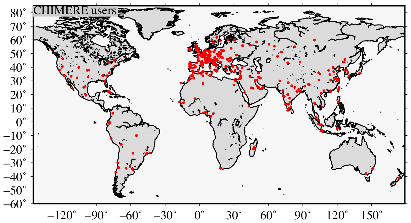
Figure 1 Map of CHIMERE users in 2021.

The previous version, called v2017r5 and distributed in 2017, was the last offline version. Its novelties were the code structure, the update, or addition of parameterizations, and the possibility to use the model with a hemispheric domain (Mailler et al., 2017). The new version presented in this article is called v2020r1 (for the year of distribution of this first release). Numerous new developments are included in this new version, and most of what is described here has already been published in articles by the CHIMERE developers. As for all previous versions, the code is open source and freely available on a website. All databases used to run simulations were also selected for their open data status. In addition to the CHIMERE code itself, this new version is also distributed with the OASIS3 – Model Coupling Toolkit (MCT) and Weather Research and Forecasting (WRF) models.

We can group and summarize these developments as follows:

1. The online coupling with WRF via OASIS3-MCT to calculate the possible retroaction of aerosols on radiation (direct effect) and cloud formation (indirect effect) (Briant et al., 2017; Tuccella et al., 2019).

2. Natural emissions: the addition of dimethyl sulfide, new schemes for sea salt, improvements of the mineral dust and biomass burning due to forest fires, NO_x by lightning (Cholakian et al., 2018; Menut et al., 2018; Menut, 2018; Turquety et al., 2020).

3. Aerosol chemistry: the addition of the volatility basis set (VBS) scheme (Cholakian et al., 2018), and the new hydrophilic/hydrophobic organics (H²O) aerosol scheme (Couvidat et al., 2012, 2018), coupled with the Secondary Organic Aerosol Processor (SOAP, Couvidat and Sartelet, 2015) thermodynamic model.

4. The subgrid-scale variability of emissions: for cells with anthropogenic emissions from several activity sectors, it is possible to have pollutant concentrations for each. This option corresponds to Valari and Menut (2010).

5. Vertical transport: updated strategy for the vertical advection of pollutants and the implementation of the Després and Lagoutière (1999) antidiffusive advection scheme, evaluated in Lachatre et al. (2020).

6. The core of the model: with the possibility to use the splitting operators or the integrated production/loss term approaches.

In this article, we summarize these new developments and show examples of their use. In order to illustrate the changes and quantify the quality of the model, we present an analysis of simulations for the entirety of the year 2014 over the Euro-Mediterranean area. Simulations, with or without new processes, one by one, are compared to measurements and to a reference case.

Section 2 presents the main novelties of this model version. Section 3 presents the simulation of the year 2014 with the model version using all new processes and updated parameterizations. This simulation is called REF. In the next sections, many other simulations are carried out in which the new parameterizations are used or not. In Sect. 5, the online developments are summarized and simulations with and without direct and indirect effects are performed. Results are compared to the REF simulation. The subgrid-scale variability of concentrations due to different activity sectors of anthropogenic emissions is described in Sect. 6. In Sect. 7, the aerosol chemistry changes are presented with the VBS and H²O schemes. The VBS scheme is described and its impact is discussed by comparing a simulation without the use of VBS to the REF simulation. The H²O scheme is summarized and its use is also compared to the REF simulation. In Sect. 8, all changes regarding the natural emissions are described: the addition of dimethyl sulfide (DMS) emissions and the improvements of sea-salt, mineral dust, and biomass burning emissions. The impacts of all the new processes are compared in Sect. 9. In Sect. 10, the code architecture changes are presented, including several optimizations, important for forecasting, and the possibility to use the operator-splitting technique for the integration of processes. The management of nesting is described in Sect. 11, and the scalability of the parallelized version is quantified in Sect. 12. Finally, a general conclusion about this new version is presented in Sect. 13.

Table 1 List of the new parameters available for the users in this model version, v2020r1.

2 What is new in v2020r1 version?

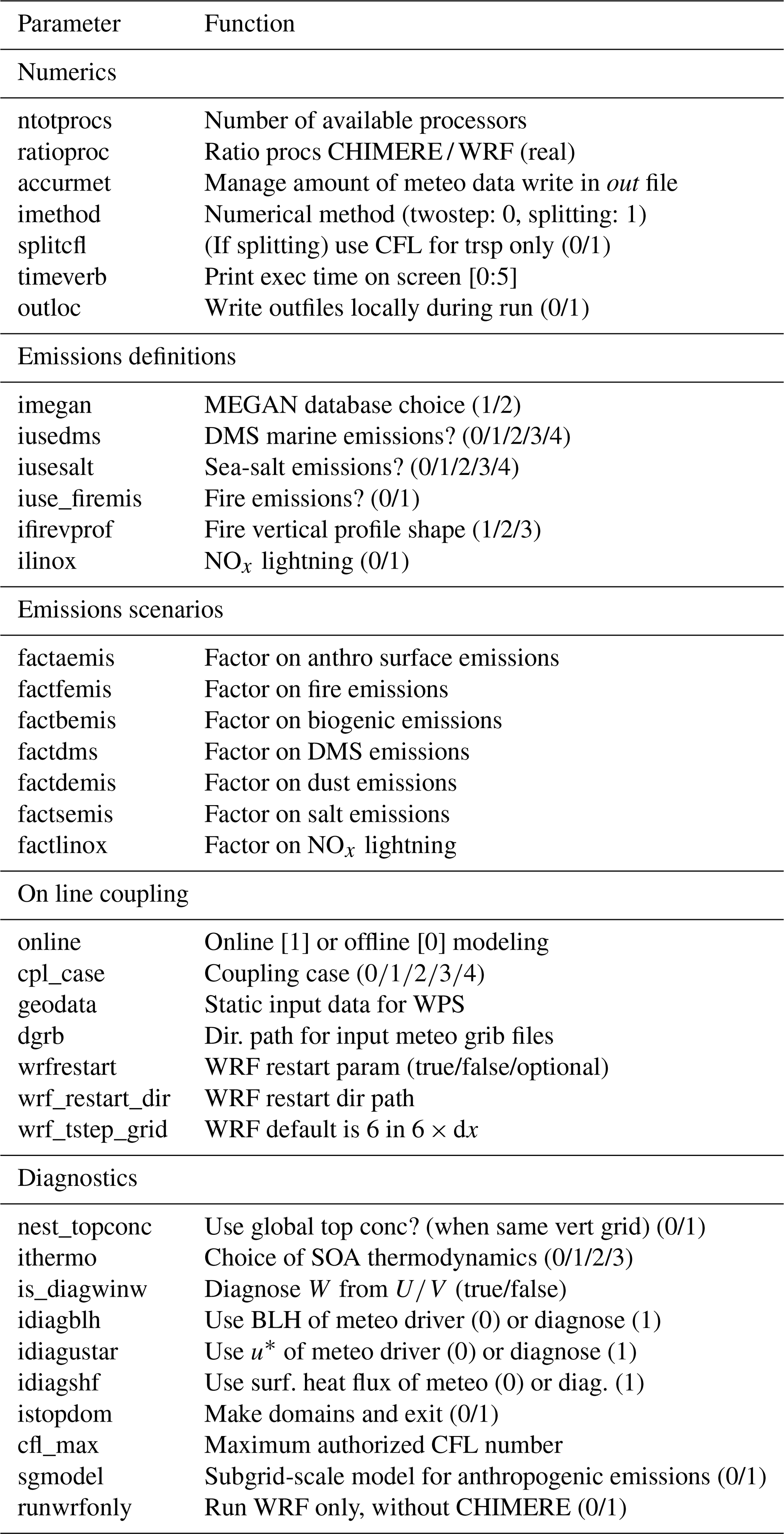
The easiest way to present the novelties of this model version is to list the new or modified users' parameters available in the simulation namelist chimere.par. The parameters and their function are summarized in Table 1.

• ntotprocs and ratioproc: with the previous offline version, the user had the possibility to specify the number of subdomains in x and y directions, and only for CHIMERE. With the online coupling in this version, two models (WRF and CHIMERE) are running at the same time and they have to share the whole amount of available processors. The user only has to specify the total number of available processors. If the user wants to favor one of the two models, it is possible to change the ratioproc value. For example, if 60 processors are available on the cluster, ntotprocs = 60 and for ratioproc = 2, 20 processors will be assigned to WRF and 40 to CHIMERE.

• accurmet: enables one to select what meteorological variables are written in the out file. Possible values are low, medium, or full.

• imethod and splitcfl: these flags are added to manage the pollutants' concentrations calculation. Historically, CHIMERE uses a method integrating all processes with a production and loss term. Many models are also using operator splitting: this later possibility was added in CHIMERE. The flag splitcfl is here to separate the time-step calculation between meteorology and chemistry when the operator-splitting technique is chosen. Details are presented in Sect. 10.2.

• timeverb: a flag to have verbose on screen, the time spent in each routine or part of the model. It is mainly for developers, i.e., if one decides to add a new parameterization in the code and wants to check the time used.

• outloc: a flag to write output results in the same directory as the executable file. Sometimes, depending on the computer architecture, writing output files on remote disks may cause instabilities and bus errors. To avoid this problem, output files are written locally, then moved to remote disks at the end of the simulation only.

• imegan: it enables one to select the land-use database used by MEGAN to calculate the biogenic emission fluxes. Two datasets are available in the CHIMERE distribution:

  • imegan = 1 for the dataset with a resolution of 2.5 min, with monthly leaf area index (LAI).

  • imegan = 2 with a resolution of 30 s and with 8 d LAI (Sindelarova et al., 2014).

• iusedms: this flag is for whether to take into account DMS emissions or not. Option 0 is for “no emissions”, and options 1, 2, 3, or 4 are to select a parameterization such as

  • iusedms = 0 (no DMS emissions);

  • iusedms = 1 (Liss and Merlivat, 1986);

  • iusedms = 2 (Wanninkhof, 1992);

  • iusedms = 3 (Nightingale et al., 2000);

  • iusedms = 4 (Elliott, 2009).

• iusesalt: like for the DMS emissions flag, this flag selects if emissions have to be taken into account (0 for “no emission”) and what parameterization to use:

  • iusesalt = 0 (no sea-salt emissions);

  • iusesalt = 1 (Monahan, 1986);

  • iusesalt = 2; (Monahan, 1986) + (Martensson et al., 2003) for the size distribution;

  • iusesalt = 3 (Martensson et al., 2003);

  • iusesalt = 4 (Grythe et al., 2014).

  More details are presented in Sect. 8.2.

• iuse_firemis and ifirevprof: these flags are for the use of fire emissions. These emissions have to be pre-calculated using external data and models. Details are provided in Sect. 8.4.

• ilinox: to take into account NO_x emissions by lightning.

• factaemis, factfemis, factbemis, factdms, factdemis, factsemis, factlinox: for all types of emissions (anthropogenic, biomass burning, biogenic, DMS, mineral dust, sea salt, and NO_x from lightning), the user can select a factor to make scenarios. Values must be real and positive, and zero is possible.

• online: the management of the coupling. It selects if the user wants a simulation in offline or online mode.

• cpl_case: type of coupling in the case of online = 1. Four possibilities are implemented:

  • 1.

    cpl_case = 1: the exchanges only go from WRF to CHIMERE. This is the same as in offline mode, except that in this case the flow is through OASIS and not by reading previously prepared WRF NetCDF files. In addition, CHIMERE receives the meteorological state at the physical time step (selected by the user and generally about 10 min) and not only hourly.

  • 2.

    cpl_case = 2: the aerosol direct effect. This case is equivalent to case 1 with, in addition to, the exchange of aerosol optical properties from CHIMERE to WRF.

  • 3.

    cpl_case = 3: the aerosol indirect effect. This case is equivalent to case 1 with, in addition to, the exchange of the cloud fraction and the droplet number from CHIMERE to WRF.

  • 4.

    cpl_case = 4: the aerosol direct and indirect effects.

• geodata, dgrb, wrfrestart, wrf_restart_dir, wrf_tstep_grid: these flags are linked to the use of WRF in online mode. They are not used in offline mode. geodata and dgrb are data paths for input data. wrfrestart and wrf_restart_dir are for the management of the restart files in the case of chained simulations. wrf_tstep_grid is a parameter to control the time step estimated for WRF and is mandatory in its namelist. In general, it is recommended to have a maximum time step, in seconds, equal to 6 × dx, with dx as the grid-cell size in kilometers. Here, the user can modulate this value.

• nest_topconc: the users can select the way to use model data at the top of the domain in the case of nesting.

• ithermo: this option is used by SOAP to compute the partitioning of semi-volatile compounds.

  • 1.

    ithermo = 1: ideal partitioning.

  • 2.

    ithermo = 2: non-ideal partitioning but without interactions with inorganic ions.

  • 3.

    ithermo = 3: non-ideal partitioning with interactions with inorganics ions. This option is used only with the H²O mechanism.

  The implementation of SOAP in CHIMERE is presented in Couvidat et al. (2018).

• is_diagwinw: originally, the vertical wind speed was diagnosed in CHIMERE from the horizontal wind components calculated by the forcing meteorological model. This is a way to ensure mass-flux consistency and therefore the conservation of mass and mixing ratio. However, as discussed in Lachatre et al. (2020), this approach introduces large errors in upper tropospheric wind, and it is possible to use directly the vertical wind speed w from the forcing meteorological model and compensate the errors in mixing ratio introduced thereby, even though this introduces errors in mass conservations. is_diagwinw = 1 corresponds to the original CHIMERE formulation, is_diagwinw = 0 to the approach described in Lachatre et al. (2020).

• idiagblh: a diagnostic report of the boundary layer height (BLH) has been available in CHIMERE for many versions. With this new option, it is now possible to select the BLH to use: in the case of coupling, the BLH calculated in WRF may be directly read and used. The way to estimate this BLH therefore depends on the user's choice with the WRF's namelist. The same is true for the diagnostic report or use of the friction velocity with idiagustar and the surface sensible heat flux with idiagshf.

• istopdom: this flag enables the creation of a horizontal domain using the WPS and WRF tools and then stop. It is useful if the user wants to check the domain before launching a simulation or use the created geography file for the calculation of surface emissions (with the emiSURF or APIFLAME programs, for example).

• cfl_max: a limit to ensure that the Courant–Friedrichs–Lewy (CFL) number is respected. The maximum is 1. But for numerical stability during horizontal transport, cfl_max = 0.8 is recommended.

• sgmodel: the subgrid-scale model for anthropogenic emissions. Note that in this case, anthropogenic emissions must be provided with activity sectors for each chemical species.

• runwrfonly: this version is being distributed with a modified version of WRF (to host the OASIS3-MCT routines for the coupling); it can be useful to have a flag to run WRF only, enjoying all the scripts already written around it (compilation, processing metgrid, geogrid, etc.)

3 The model setup for its evaluation

3.1 Model setup

Several model configurations are defined in order to answer the following questions:

1. Is this version more accurate than the previous one? To answer this, two simulations are performed: one with the previous version (v2017r5) and one with the new version (v2020r1). In order to have a correct comparison, v2020r1 is used in offline mode and the two versions are forced by the ECMWF meteorological fields to achieve data assimilation of meteorological variables.

2. What is the impact of the coupling on the results? Even if using coupling is, by principle, more realistic, it is interesting to quantify how this coupling changes the modeled concentrations. Four simulations are carried out: using the offline mode (cpl_case = 1) and the online mode with only direct effects (cpl_case = 2), only indirect effects (cpl_case = 3), and all effects (cpl_case = 4).

3. What is the impact of the new schemes implemented in this model version? Is there one process largely changing the results? Several simulations are also performed with a single main configuration and the processes are changed one by one.

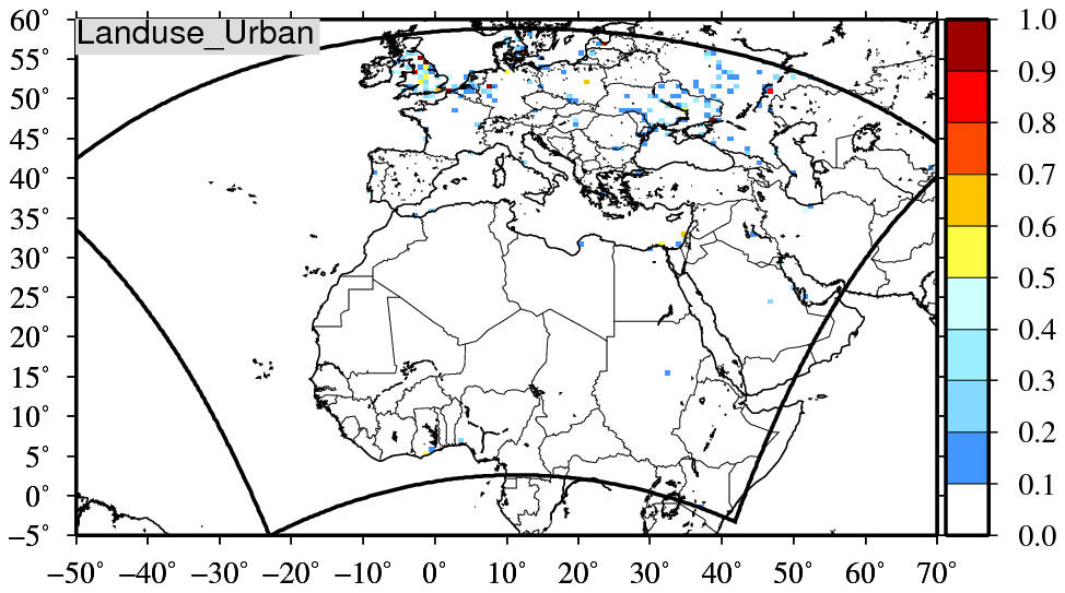
Figure 2 Map of the studied region with the modeled domain. The colors represent the percentage of urban and built-up surfaces in each model cell.

For all simulations, the domain was chosen to be large enough to take into account all kinds of possible sources (Fig. 2). By including the northern half of Africa and Europe, the modeled region is able to take into account anthropogenic, biogenic, biomass burning, sea-salt, and dust sources, with a horizontal resolution of 60 × 60 km. The whole year of 2014 was modeled.

3.2 The observations used for validation

The model was validated by using a vast dataset of atmospheric and meteorological in situ measurements. The European Environment Agency (EEA, https://www.eea.europa.eu, last access: 6 September 2021) provides hourly data for a list of atmospheric species and a substantial number of stations covering Europe, categorized by station type (rural, traffic, etc.). The data for particulate matter PM_2.5 and PM₁₀, ozone (O₃), and nitrogen dioxide (NO₂) are used for regular model validations and are presented in this article. The number of stations differ for each pollutant; for the year of 2014, the data from 322 stations for NO₂, 431 stations for O₃, 178 stations for PM₁₀, and 69 stations for PM_2.5 are used in our comparisons. We have also included aerosol optical depth (AOD) data taken from the AErosol RObotic NETwork global remote sensing network (AERONET, https://aeronet.gsfc.nasa.gov/, last access: 6 September 2021). Out of the 305 stations in the network having measurements for the year 2014, 75 are in the simulation domain and are used for the validation shown in this paper.

We have also included validation for vertical profiles of pressure, temperature, and ozone using the data downloaded from the World Ozone and Ultraviolet Radiation Data Centre (WOUDC, https://woudc.org/home.php, last access: 6 September 2021) resulting from ozonesonde measurements. The database used is the one of July 2021. From around 25 stations that are in our domain, only nine have consistent data for the year 2014. All nine stations use an electrochemical concentration cell (ECC) as the measurement instrument (https://woudc.org/data/instruments/, last access: 6 September 2021). Out of the remaining nine stations, seven of them are well allocated over the seasons of the year, each representing at least 10 sondes per season. The two remaining stations, in Ireland and Italy, have 24 and 28 usable sondes, respectively. These two stations present data only for the winter months. Our criteria for choosing the stations was their geographical position: we wanted to present different parts of Europe in the limits of availability of data for the stations; therefore, the stations in Ireland, Switzerland, and Poland were chosen in the presentation of the results. The number of total sondes over all the stations (561 in total) and their temporal distribution over different seasons are quite enough to be representative of both the geographical and temporal aspects of the simulations.

Meteorological parameters have also been validated using two datasets. The ECA&D project provides the E-OBS database containing measurements for a large number of stations over the European region. This dataset provides values for daily temperature (average, minimum, and maximum), daily average wind speed and direction, relative humidity, and precipitation; the data can be downloaded both in a gridded format or per station files. The data provided by the British Atmospheric Data Centre network (BADC, http://data.ceda.ac.uk/badc, last access: 6 September 2021) is also integrated into the validation chain, providing hourly values for temperature, wind speed, and precipitation. While these results are not presented in this article, they are checked in regular validation processes performed for all simulations.

All datasets are integrated into the evaltools Python package (https://opensource.umr-cnrm.fr/projects/evaltools, last access: 6 September 2021, version 1.0.6r) which is designed as a free assessment tool for atmospheric models versus in situ observations. Given the output for all simulations and all the observations, this tool provides a statistical comparison between the aforementioned simulations and the provided measurements. The tables and images presented in this paper are all produced by this tool.

4 Improvement of v2020r1 compared to v2017r5

In order to quantify the quality of this new version, two simulations are performed: one with v2017r5 and one with v2020r1. The meteorology used corresponds to the IFS/ECMWF fields, with a global $\mathrm{0.25}{}^{\circ }\times \mathrm{0.25}{}^{\circ }$ resolution and 3-hourly time frequency. For each day, we use an analysis day of this dataset. The new version is used in offline mode to be homogeneous with the v2017r5 version.

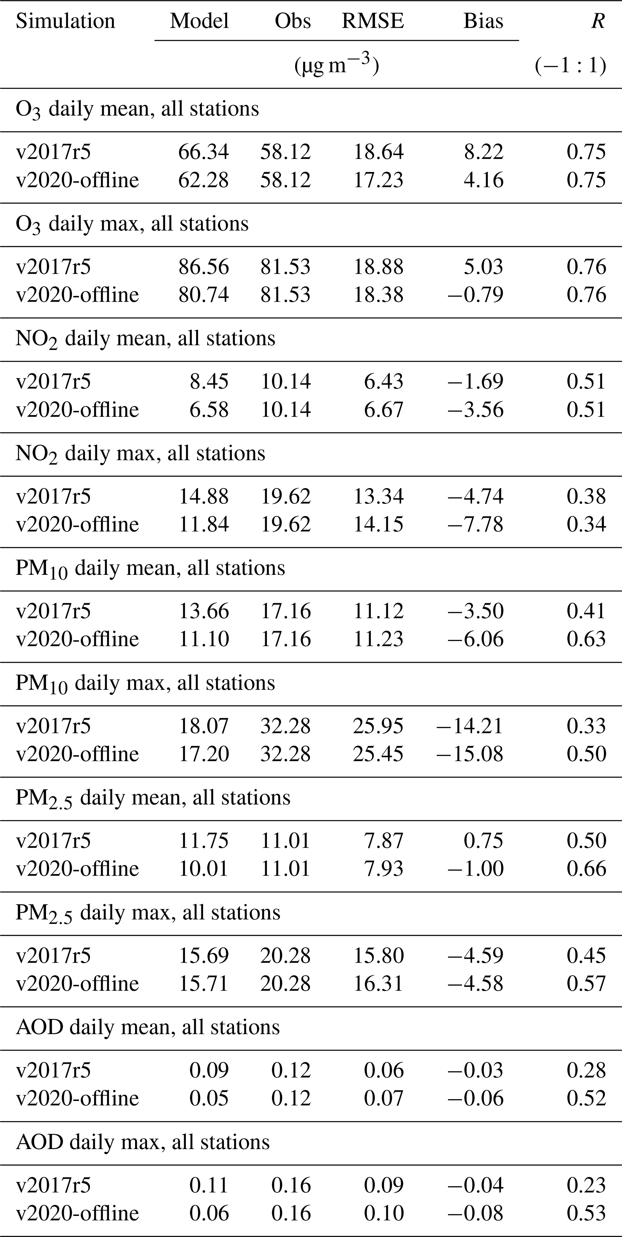
Table 2 Main results for the v2017r5 and v2020r1 versions of the CHIMERE model. Scores are calculated by comparison between surface observations for several stations in Europe and the corresponding model daily mean and maximum value. Statistical scores are presented for O₃, NO₂, PM₁₀, PM_2.5, and AOD.

4.1 Statistical scores

Results are presented in Table 2 for the daily mean and maximum values of O₃, NO₂, PM₁₀, PM_2.5, and AOD. Due to the horizontal resolution of the simulations (Δx=60 km), and to the representativity of the model outputs compared to the measurements, the scores are presented for “rural” stations.

For surface ozone mean concentrations, the correlations are high in the two cases (0.75) but there is no improvement with the new version. There is an improvement for the bias, reduced from 8.22 to 4.16 µg m⁻³ with the V2020r1 version. For the daily maxima, the correlation is the same (0.76) and the bias is also reduced (−0.79 in place of 5.03 µg m⁻³). For NO₂ surface concentrations, the scores have not improved with the v2020r1 version. The bias increased, and the correlation for the mean values is 0.51 with the two versions. But knowing the horizontal resolution of the simulations, it is not unexpected to not have very good scores for NO₂, a species mainly emitted in urban areas and with strong horizontal gradients.

On the other hand, results have really improved for particulate matter (PM) and AOD. For the PM₁₀ mean and maximum daily values, the correlation between the models' outputs and observations increased from 0.41 to 0.63 (mean) and 0.33 to 0.50 (max), respectively. The same kind of improvement is noted for PM_2.5. For AOD, the correlations increased from 0.28 to 0.52 for the daily mean and from 0.23 to 0.53 for the daily maximum. If the bias is reduced with the new version for PM, it increases for AOD.

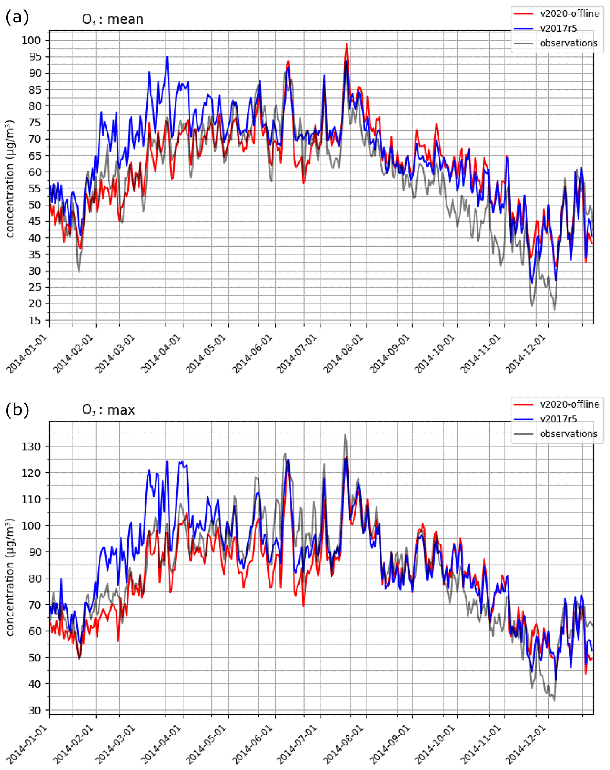
Figure 3 Time series of daily mean (a) and maximum (b) ozone surface concentrations measured with the European Monitoring and Evaluation Programme (EMEP) network and modeled with CHIMERE v2017r5 and v2020r1.

4.2 Time series of O₃

Time series are presented in Fig. 3 for ozone daily mean and daily maximum surface concentrations (in µg m⁻³). Data are averaged in time, but also spatially, over all model cells where European Monitoring and Evaluation Programme (EMEP) data are present. For mean or maximum values, the behavior of the modeled concentrations compared to observations is close: the two model versions are able to catch the annual cycle, as well as the major observed peaks. For the spring of 2014, the v2020r1 version is more able to model the observed concentrations, when v2017r5 overestimates the values. During the summer, the two versions give good results in the both cases. For autumn and winter of 2014, the two versions are also close but overestimate the concentrations.

Figure 4 Time series of surface ozone daily exceedances, measured with the EMEP network and modeled with CHIMERE v2017r5 and v2020r1.

4.3 Daily peaks

As the CHIMERE model is being extensively used by organizations for daily forecasting, it is useful to add calculations with the capability to model daily peaks of the pollutants' surface concentrations (such as ozone, NO₂, particulate matter). An example is presented in Fig. 4 with the count of exceedances of 180 µg m⁻³ for the daily maximum for surface ozone concentrations. With the observations, two major peaks are recorded: 10 June and 22 July 2014. Four to five other less numerous peaks were also recorded. For the peak on the 10 June, 23 stations recorded an exceedance in western Europe. Model v2020r1 was able to reproduce 15 exceedances, whereas v2017r5 was only able to reproduce 2. For the peaks on 22 July, 15 exceedances are observed, 15 are modeled by v2020r1, 12 by v2017r5. For these two cases, the v2002r1 version improves the capability of the model to simulate ozone daily maximum surface concentrations.

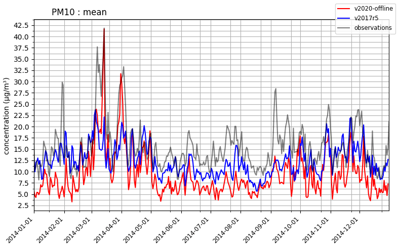
Figure 5 Time series of PM₁₀ daily mean surface concentrations measured with the EMEP network and modeled with CHIMERE v2017r5 and v2020r1.

4.4 Time series of PM₁₀

The time series of surface concentrations of PM₁₀ is presented in Fig. 5. The two model configurations are able to simulate the annual variability of particulate matter to the same order of magnitude. The new version gives lower values than v2017r5 but with a better day-to-day variability (correlation shown in Table 2).

Table 3 O₃ vertical profile results for the v2017r5 and v2020r1 versions of the CHIMERE model. Scores are calculated by comparison between ozonesonde observations and the corresponding model vertical distribution of ozone. Statistical scores are presented for O₃; correlations for each model level are shown in Fig. 6. The coordinates and the number of sondes are given on top of each column.

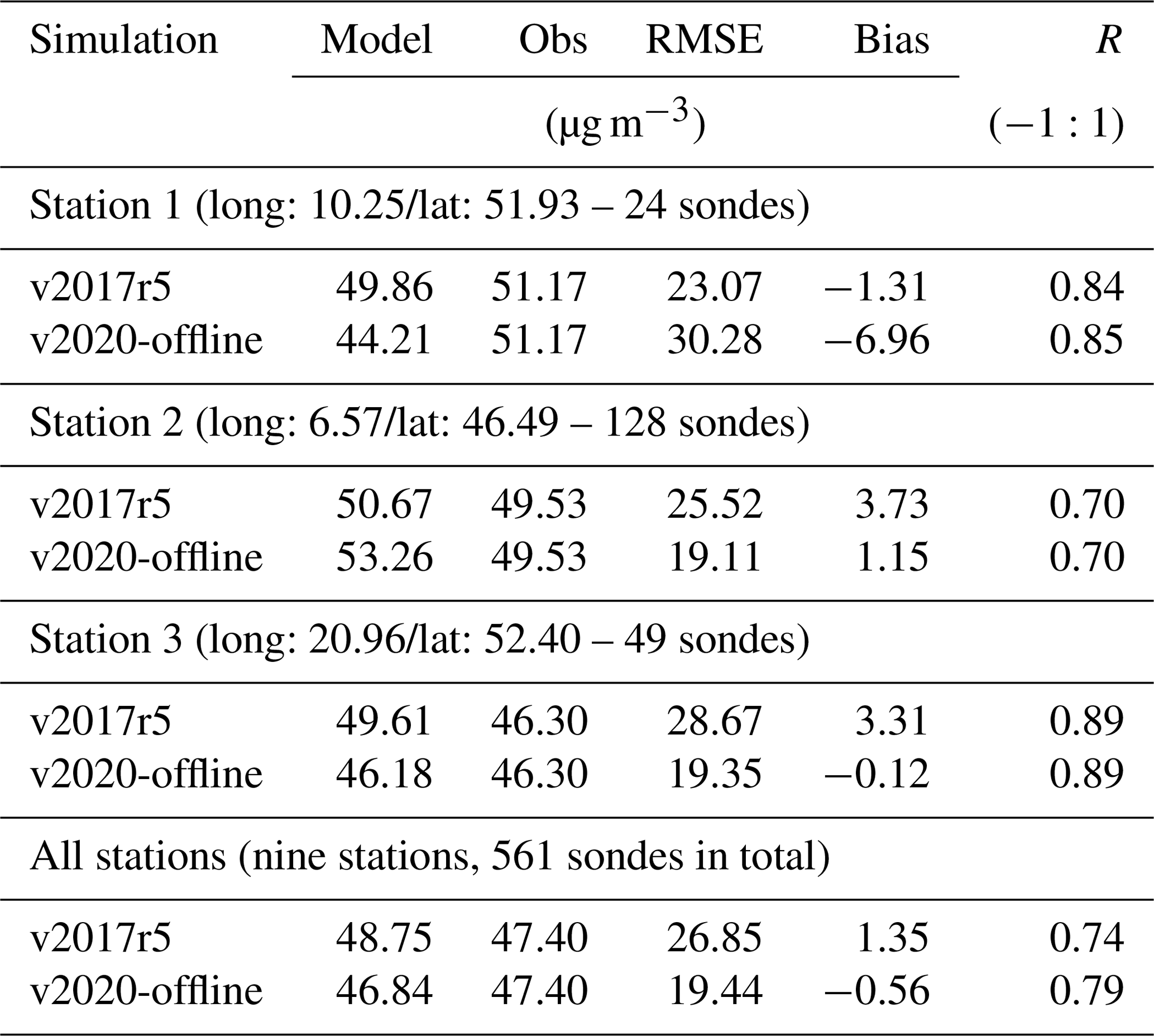
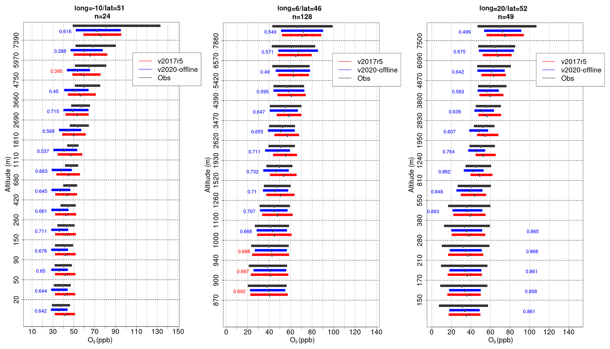
Figure 6 O₃ vertical profiles for three stations across Europe. Coordinates of the stations are given at the top of each plot. Each bar represents the spread (10 % to 90 % quantiles) of the data for the two versions (blue and red) and observations (gray). The value on each level represents the correlation for the model with the higher correlation with the same color. The small white dot on each bar represents the average.

4.5 Vertical profiles of O₃

Apart from surface measurement validations, we have also included a vertical profile comparison between v2017r5 and v2020r1. Since the model is used for national air quality forecast simulations, it is important to have a good vertical representation for species commonly used as air quality indicators, such as O₃. The measurements used are explained in Sect. 3.2. While nine stations are available in our simulation domain (with 561 sondes in total during the year 2014), three of them were chosen to be shown in this article. The choice of these stations was done on the basis of their location in an effort to cover different regions of the European continent. The O₃ vertical profiles of the chosen stations are shown in Fig. 6, while the locations and statistics for each one are shown in Table 3. The figures show the spread of all sondes for each station over the year 2014 for each level of the model.

For these three stations, the two versions are quite close when it comes to simulating the shape of vertical variations, the order of magnitude of concentrations, and near-surface concentrations of O₃. The statistics for these stations are also quite similar on average, although the bias presented by v2020r1 shows improvements. However, the higher in altitude the model level is, the more visible the differences between the two versions become: at most stations, 2020r1 manages to simulate higher altitudes better regarding the correlation, spread of the concentrations, and bias. This is especially visible looking at the correlation of each level shown in Fig. 6, which in the majority of cases is higher for v2020r1 compared to 2017r5. The average statistics for all stations are also included at the end of Table 3, showing general improvement on correlation, bias, and RMSE in v2020r1.

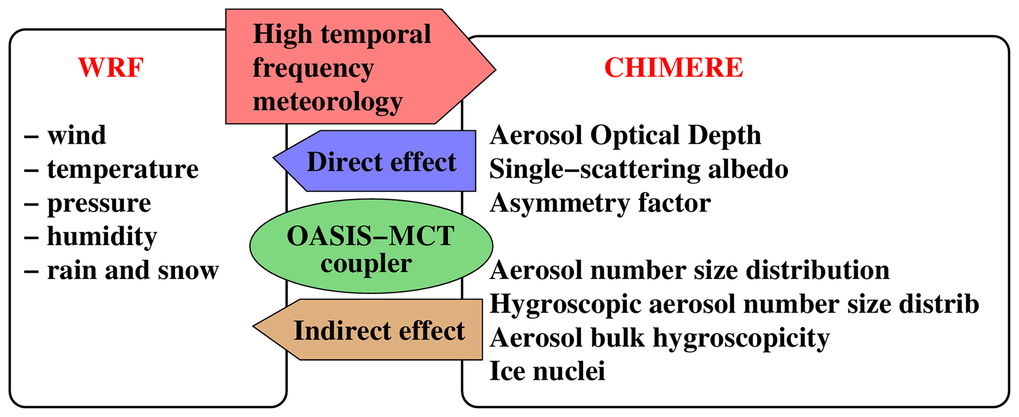
Figure 7 Main principle of the coupling between WRF and CHIMERE for the calculation of the direct and indirect effects of aerosols on meteorology.

5 Impact of the online coupling

In this section, only the v2020r1 version is used. Sensitivity tests are performed using several options of the online coupling to quantify its impact on the results. The same setup is used from the validation: the large domain with 60 × 60 km resolution over Africa and Europe, and the complete simulation of the year 2014.

Online models are dedicated to take into account the retroaction between radiation, clouds and aerosols in the atmosphere (Zhang, 2008; Baklanov et al., 2014). The model developed here is in the category online access model and couples the Weather and Research Forecasting (WRF) (Powers et al., 2017) and CHIMERE (Mailler et al., 2017) regional models with the OASIS3-MCT coupler (Craig et al., 2017). Two kinds of retroaction are considered: the direct and the indirect effects, respectively, detailed for WRF-CHIMERE in Briant et al. (2017) and Tuccella et al. (2019). The variables exchanged between the two models are described in Fig. 7. The exchange frequency ranges from 1 to 30 min, depending on the horizontal resolution and the user's choice.

The meteorology is calculated using the version 3.7.1 of WRF and with a configuration identical to the one used in Menut et al. (2018). The model uses spectral nudging to follow the large scale dynamics (Von Storch et al., 2000). The National Centers for Environmental Prediction (NCEP) fields are nudged for pressure, temperature, humidity, and wind and for wavelengths greater than ≈ 2000 km and only for pressure above 850 hPa. The WRF model thus remains free to create its own dynamics in the boundary layer. This configuration allows the regional model to create its own dynamics within the boundary layer. The large scale follows the thermodynamics fields from the NCEP analyses.

For the model distribution, note that, for the first time, CHIMERE is distributed with OASIS3-MCT3.4 and WRF v3.7.1. OASIS is used as is but WRF was modified in order to be able to receive data via the OASIS coupler.

5.1 Direct effects

The direct effect impacts the thermodynamics below an aerosol layer after scattering and absorption of solar radiation (Haywood and Boucher, 2000; Helmert et al., 2007; Zhang, 2008). To take into account this effect, the CHIMERE model calculates AOD, single scattering albedo (SSA), and an asymmetry factor and sends it to WRF (in place of the climatology used by the meteorological model when it is used alone). This new information varies every physical time step (i.e., a few minutes) and are used in WRF by the Rapid Radiative Transfer Model for GCM (RRTMG) scheme (Iacono et al., 2008).

5.2 Indirect effects

The implementation of the indirect effect in WRF and CHIMERE was performed and presented in Tuccella et al. (2019). The indirect effect takes into account the aerosol-induced increase in cloud condensation nuclei (CCN) and ice nuclei (IN), and the subsequent changes in clouds microphysical and optical properties. An increase of CCN induces for cloud with the same liquid water path, an enhancement of cloud albedo due to a larger droplet number with smaller dimensions (first indirect effect or Twomey's effect). A variation in CCN burden induces also changes in cloud lifetime and precipitation pattern (second indirect effect or Albrecht effect) (Andreae and Rosenfeld, 2008).

The microphysics parameterization used in WRF is the aerosol-aware scheme of Thompson and Eidhammer (2014). This scheme calculates the cloud droplet nucleation rate using the aerosol size distribution calculated in CHIMERE. The activation scheme of Thompson and Eidhammer (2014) is replaced by the one of Abdul-Razzak and Ghan (2002), the latter being able to use a sectional approach for aerosols as designed in CHIMERE. For each aerosol section, the scheme is able to calculate the fraction of activated aerosol. For the cloud ice formation, it is calculated in the Thompson and Eidhammer (2014) scheme, and the climatology of IN is replaced by the IN concentration diagnosed in CHIMERE. The scheme for the ice nucleation is the one of Tobo et al. (2013), corresponding to an adaptation of DeMott et al. (2010).

Some aerosol properties are calculated in CHIMERE for the indirect effects and are sent to WRF, to be read in the Thompson and Eidhammer (2014) microphysics scheme. The number concentrations, N_i (m⁻³), of all aerosols (except water) and for each size distribution bin i, are defined as

$$\begin{array}{}\text{(1)}& N_i=\sum _{\mathrm{a}=\mathrm{1},\mathrm{naero}}{\displaystyle \frac{c_{i,\mathrm{a}}\times {\mathrm{10}}^{-\mathrm{9}}}{{\mathrm{vol}}_i\times {\mathit{\rho }}_{\mathrm{a}}}},\end{array}$$

with c_i,a the mass concentration of each “a” aerosol and bin i (µg m⁻³), vol_i (m³) the volume of the aerosol in the bin i, and ρ_a (kg m⁻³) the density of aerosol “a”. A subset of N_i, called N_i,hygro, is calculated in the same way but only for hygroscopic aerosols (salt, SOA, H₂SO₄, NH₃, and HNO₃). The aerosol bulk hygroscopicity, H, is estimated as

$$\begin{array}{}\text{(2)}& H_i={\displaystyle \frac{{\sum }_{a=\mathrm{1},\mathrm{naero}}\left(\frac{H_{\mathrm{a}}\times c_{i,\mathrm{a}}}{{\mathit{\rho }}_{\mathrm{a}}}\right)}{{\sum }_{a=\mathrm{1},\mathrm{naero}}\left(\frac{c_{i,\mathrm{a}}}{{\mathit{\rho }}_{\mathrm{a}}}\right)}},\end{array}$$

where the H_a hygroscopicity factors are expressed for each aerosol as in Table 4. IN (m⁻³) are estimated with mineral dust concentration only and for the size distribution part corresponding to a mean mass median diameter D>0.5 µm, as

$$\begin{array}{}\text{(3)}& \mathrm{IN}=\sum _{i=\mathrm{1},D_{\mathrm{p}}>\mathrm{0.5}\mathrm{\mu }\mathrm{m}}{\displaystyle \frac{c_{i,\mathrm{dust}}\times {\mathrm{10}}^{-\mathrm{9}}}{{\mathrm{vol}}_i\times {\mathit{\rho }}_{\mathrm{dust}}}}.\end{array}$$

Table 4 Hygroscopic properties of the aerosols modeled in CHIMERE.

The developments in this model version may induce a slight underestimation of the cloud formation regarding the indirect effects. It is due to the fact that the Thompson and Eidhammer (2014) microphysics scheme only takes into account grid-resolved clouds. The diagnostic of these grid-resolved clouds depends on the horizontal resolution. For a coarse resolution, they are less well calculated than for a fine resolution. In addition, some clouds may be generated by convection, as described in the Grell and Freitas (2014) scheme used in WRF. But, for this coupled version, this effect is not yet implemented (as in many regional models) and this will be the subject of future developments.

The use of the direct and indirect effects is up to the user's discretion, with two flags called online and cpl_case. When online is equal to 1, the model considers the values of cpl_case, the several degrees of the coupling.

For cpl_case = 1, there is no aerosol feedback from CHIMERE to WRF, but the meteorological parameters are sent from WRF with the coupling time step. This is still a step forward when compared to the previous CHIMERE versions which were only able to read hourly meteorological outputs. For cpl_case = 2, only the direct effects are taken into account. For cpl_case = 3, only the indirect effects are taken into account. With cpl_case = 4, the direct and indirect effects are both taken into account.

5.3 Results

To illustrate the coupling, five simulations were performed with and without direct and indirect effects. These simulations correspond to the following:

1. offline-wrf: the CHIMERE model is forced by hourly meteorological fields stored in the WRF model output files (as in the previous CHIMERE version). It corresponds to option online = 0.

2. cpl1: there is no coupling but CHIMERE received WRF meteorological fields using the OASIS-MCT coupler. The coupling frequency is now the physical time step (for example, 15 min).

3. cpl2: coupling with the aerosol direct effect.

4. cpl3: coupling with the aerosols indirect effect.

5. cpl4: coupling with the direct and indirect effects.

WRF and CHIMERE use the same horizontal domain and the same grid size of 60 km × 60 km resolution to avoid horizontal interpolation during the coupling. The output results are issued hourly. The modeled period ranges for the whole year of 2014, like in the previous sections.

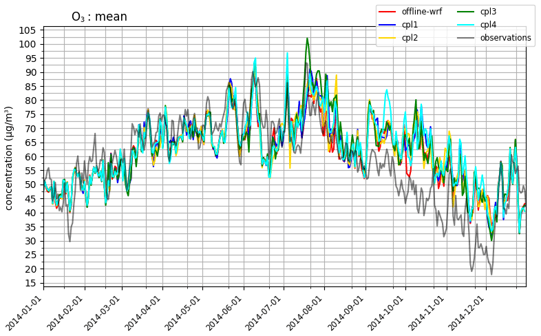
Figure 8 Time series of ozone surface concentrations measured with the EMEP network and modeled with CHIMERE v2020r1 for cpl_case = 1, 2, 3, and 4.

Results are presented in Fig. 8. For the “offline-wrf” simulations, CHIMERE is forced by previously calculated WRF meteorological fields, themselves forced by NCEP. For “cpl1”, CHIMERE is forced by WRF meteorological fields calculated independently of CHIMERE (with no retroaction from CHIMERE to WRF). The main differences between the two simulations are (i) the meteorological fields are read in through a file in the first case but sent by OASIS3-MCT in the second case, (ii) more importantly, the meteorological fields forced CHIMERE hourly with “offline-wrf”, when with “cpl1”, it is at each physical time step (in this case, 20 min). As previously shown in Briant et al. (2017), having more frequent meteorological fields presents a very important effect on results: temperature is more precise for photolysis, surface wind fields are more accurate for natural emissions, etc. All configurations show an overestimation of the ozone daily mean concentration, with a bias between 3 and 4 µg m⁻³, compared to observations. The variability between the several model configurations is only 1 µg m⁻³, showing that the choice of the coupling is not the main reason for the bias.

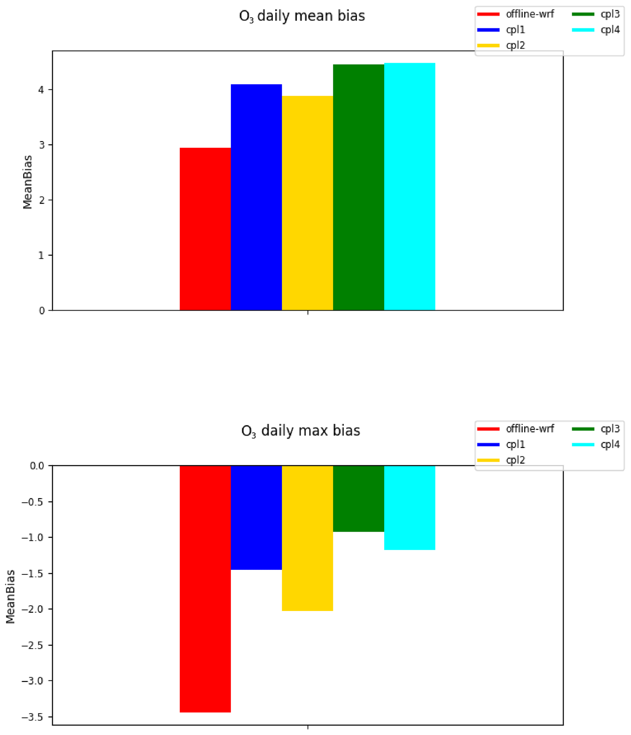
Figure 9 Bias (model–obs) in µg m⁻³ with CHIMERE v2020r1 for offline mode and online with cpl_case = 1, 2, 3, and 4. Scores are calculated for the whole year and over the whole domain, for model cells where observations data are present and valid.

In order to quantify the differences between the simulations, the daily mean and max biases are presented in Fig. 9. Results show the bias increases with the coupling for the mean ozone concentrations values. But for the daily maximum ozone values, the bias decreases. The use of the online coupling is more realistic but may be also an improvement for the forecast, when searching for exceedances based on threshold values.

Statistical scores for these simulations are also presented in Table 5. For NO₂, the bias remains the same and decreases for PM₁₀ but increases for PM_2.5. For the correlation, the results show low changes among the different configurations. This means that the online coupling is an improvement for modeling realistic physicochemical interactions but is not a major change on average for surface pollutant concentrations.

Table 5 Main results for the different coupling options of the v2020r1 CHIMERE version. Scores are calculated by comparison between surface observations for several stations in Europe and the corresponding model daily mean value. Statistical scores are presented for O₃, NO₂, PM₁₀, PM_2.5, and AOD.

6 A subgrid-scale model to account for heterogeneous surface emissions

Regional-scale chemistry-transport models such as CHIMERE do not resolve physical and chemical processes occurring at spatial scales below 1 km². If such effects are to be accounted for, they must be parameterized. Heterogeneous surface emissions at the unresolved subgrid scale (i.e., at spatial scales smaller than the model resolution) have been shown to have a large impact on grid-averaged pollutant concentrations (Galmarini et al., 2008; Valari and Menut, 2010; Korsakissok and Mallet, 2010; Cassiani et al., 2010). Especially over urban areas with large population density, very contrasted emission sources, such as roads and buildings coexist within small distance. To account for this subgrid-scale effect, the new version of CHIMERE includes the scheme described in Valari and Menut (2010), following which the CHIMERE model grid-cell area is divided into several subgrid areas, each representing a different emission source. During the CHIMERE simulation, at each model time step, the calculation of chemistry splits into the different subgrid volumes.

Figure 10 The 10 d hourly time series of modeled and measured NO₂ (µg m⁻³) surface concentrations. The top panel compares simulations with observations over a traffic monitor site, while the bottom panel over a background monitor site of the AIRPARIF air quality network. Concentrations are simulated with the usual CHIMERE calculation where emissions are homogeneous over the grid-cell volumes (black lines) and with the “on-road” component of the subgrid-scale model.

The subgrid-scale model produces surface concentrations for all model species at each model time step. Figure 10 compares simulated hourly concentrations over two surface stations in the city of Paris with (i) the usual CHIMERE calculation and (ii) the “on-road” component of the subgrid-scale module against surface measurements of the AIRPARIF local regional air quality network. A traffic site (OPERA) and an urban background site (PA04C) are chosen for these comparisons as shown in Fig. 10. It is shown that the “on-road” component of the subgrid-scale simulation models significantly higher NO₂ levels compared to the grid-averaged value especially during rush hour. On the contrary, as expected, over the urban background monitor site, the grid-averaged concentration is generally closer to observations.

7 Secondary organic aerosol (SOA)

The secondary organic aerosol calculations changed a lot with this model version. Mainly, two different schemes were added: the H²O (hydrophilic/hydrophobic organics) mechanism (Couvidat et al., 2018) and the VBS scheme (Zhang et al., 2013), with a version including the fragmentation process (Cholakian et al., 2018).

7.1 The several mechanisms

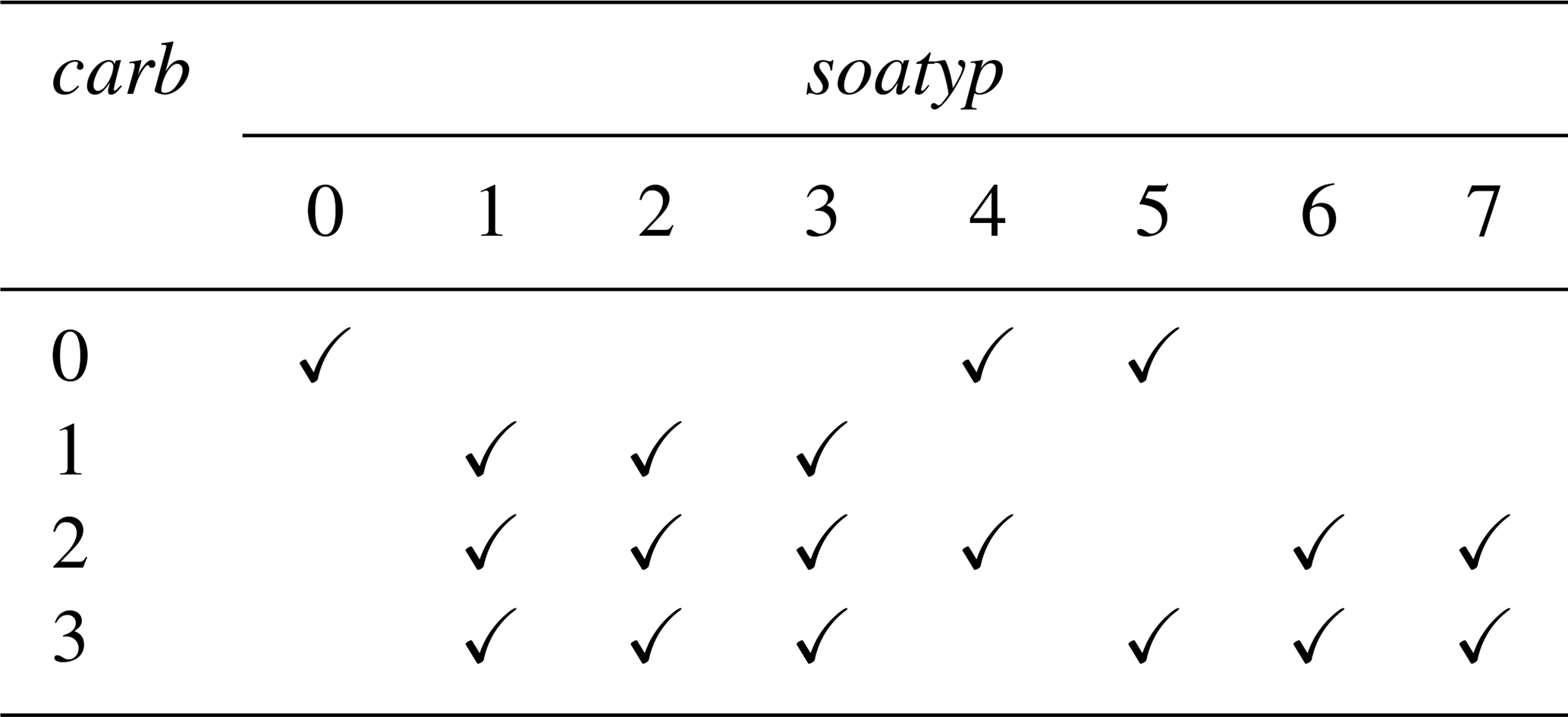
There are two different choices available for SOA modeling. The first one is the flag carb and is linked to the anthropogenic emitted species list. The second one is the flag soatyp for the parameterization of SOA formation. The two flags are linked.

The values of carb are

• carb = 0: no primary carbonaceous species.

• carb = 1: primary carbonaceous species (OCAR and BCAR) are used.

• carb = 2: primary carbonaceous species (POA and BCAR) are used. With VBS, POAs (POA + IVOC + SVOC) are separated into nine volatility bins. Only the functionalization process is taken into account (Zhang et al., 2013). With H²O, POAs are split into three compounds (POAlP, POAmP, and POAhP) with, respectively, low, medium, and high volatilities.

• carb = 3: primary carbonaceous species (POA and BCAR) are used. POAs (POA + IVOC + SVOC) are separated into nine volatility bins. Functionalization, fragmentation, and non-volatile bins are taken into account (Cholakian et al., 2018). With H²O, POAs from biomass burning are separated into three species (BOAlP, BOAmP, and BOAhP) using a specific split. Other POAs are distributed into POAlP, POAmP, and POAhP compounds.

Table 6 List of anthropogenic emitted species depending on the way to split the emissions of primary particulate matter (PPM) and the chemical scheme used for the SOA formation.

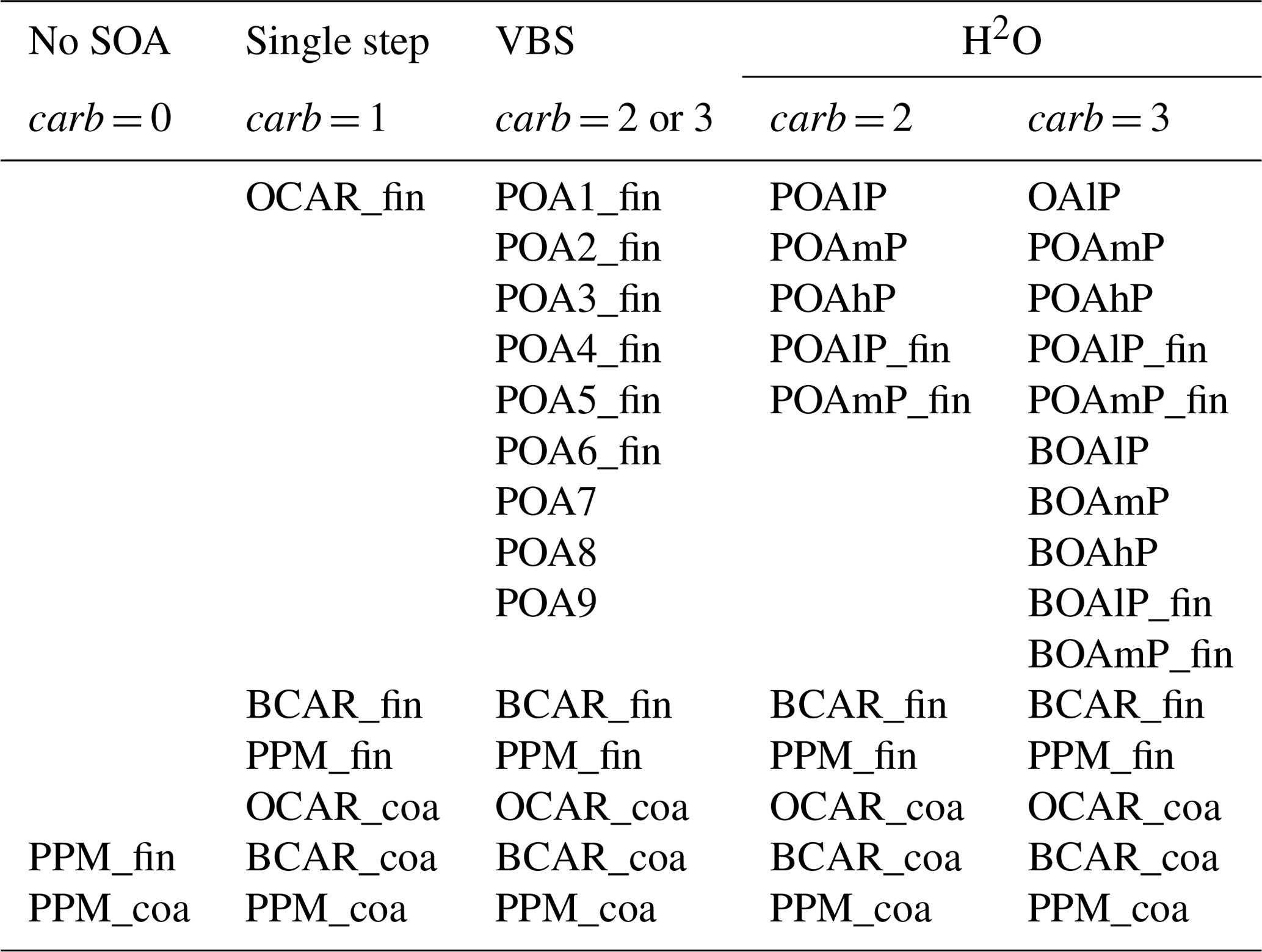
The emitted species used, depending on carb, are listed in Table 6. For carb = 0, there is no speciation between OCAR and BCAR. The model only uses PPM as emission, without chemistry. With carb = 1, PPM is separated into OCAR, BCAR, and PPM. This is done with the anthropogenic emissions program emisurf, distributed with CHIMERE. For users that have their own anthropogenic interface, it is required to build emissions with this speciation.

The values of soatyp are

• soatyp = 0: no SOA chemistry;

• soatyp = 1: single-step oxidation (simple);

• soatyp = 2: single-step oxidation (medium);

• soatyp = 3: single-step oxidation (complex);

• soatyp = 4: H²O (hydrophilic/hydrophobic organics) mechanism (Couvidat et al., 2018);

• soatyp = 5: H²O reduced mechanism (Couvidat et al., 2018);

• soatyp = 6: VBS scheme (Zhang et al., 2013);

• soatyp = 7: VBS scheme with fragmentation process. (Cholakian et al., 2018)

Note that for single step, VBS, or H²O, the biogenic VOC precursors emitted by MEGAN are taken into account: APINEN (α-pinene and sabinene), BPINEN (β-pinene and δ³-carene), LIMONE (limonene), OCI (myrcene and ocimene), and C₅H₈ (isoprene).

When selecting the carb flag, it is important to be consistent with the choice made for this variable in the emisurf program/namelist if the user is using this tool.

Depending on the choice of VBS, the anthropogenic emissions of PPM are separated into several emitted species or not. The first level of separating is to distinguish between organic carbon (OCAR) and black carbon (BCAR) in the fine mode (“_fin”). The possible sets of values for carb and soatyp are explained in Table 7. Note that it is possible to use carb = 0 and soatyp = 4 or 5. In this case, POAs are not used to estimate the relative part of organics in SOAP (see Couvidat et al., 2018 for details).

Table 7 Correspondence between the different carb and soatyp flag values.

7.2 Single-step oxidation mechanism

For soatyp equal to 1, 2, or 3, the formation of SOA is taken into account with single-step oxidation schemes. Anthropogenic precursors include

• TOL (benzene, toluene, and other mono-substituted aromatics),

• TMB (trimethylbenzene and other poly-substituted aromatics), and

• NC4H10 (higher alkanes).

The base SOA module was tested against the smog chamber data of Odum et al. (1997) for anthropogenic compounds and those of Griffin et al. (1999) for biogenic compounds, and was shown to satisfactorily reproduce SOA formation for these compounds. Higher alkanes and isoprene were added to the original chemical mechanism of Pun et al. (2006). The formation of SOA from higher alkanes follows the formulation of Zhang et al. (2007) for the stoichiometric SOA yield, and it is assumed that the SOA species can be represented by a hydrophobic surrogate compound with moderate saturation vapor pressure. The formation of SOA from the oxidation of isoprene by hydroxyl radicals is represented with two surrogate products and follows the formulations of Kroll et al. (2006) and Zhang et al. (2007).

7.3 The H²O mechanism

The H²O mechanism is presented in detail in Couvidat et al. (2012), and its performance was evaluated over Europe in Couvidat et al. (2018). This mechanism is an evolution of the Pun et al. (2006) mechanism. It uses the molecular surrogate approach, into which semi-volatile organic compounds with similar thermodynamical properties are lumped together and are represented with a single molecular structure. By attaching a molecular structure to the surrogate structure, several processes can be represented that are often not taken into account. For example, absorption of organic compounds into the aqueous phase of aerosols, the acidic dissociation, and non-ideality (interactions between organic compounds and with inorganics compounds) can be estimated. The model distinguishes two types of compounds: hydrophilic compounds (compounds with a high affinity for water that can condense into the aqueous phase of particles) and hydrophobic compounds (compounds with a low affinity for water that condense into an organic-rich phase).

The mechanism takes into account SOA formation from the oxidation of isoprene, monoterpene, sesquiterpenes, and aromatic compounds. The properties of the surrogate compounds are described in the parameter file species.cxx and are summarized in Table 2 of Couvidat et al. (2018). It should be noted that some compounds (like AnClP or POA) do not have a predefined molecular structure. In that case, a hydrophobic default structure is used.

The complete mechanism (soatyp = 4) has 15 species and has been reduced to 7 species (soatyp = 5). Contrary to the other SOA mechanisms, equilibrium is computed with SOAP to account for non-ideality and aqueous-phase absorption. ithermo in chimere.par must be above 1.

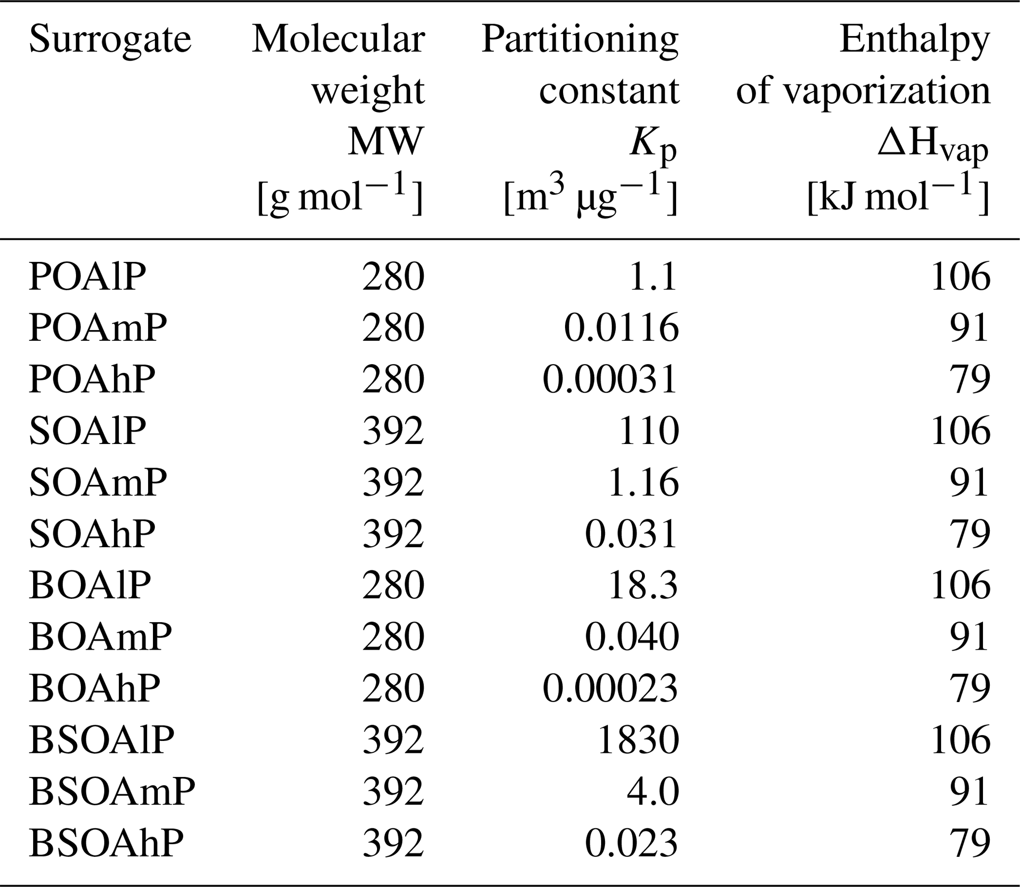
POA can be considered as semi-volatile within H²O with the option carb equal to 2 or 3 in chimere.par. With carb equal to 2, POAs are split into three compounds: POAlP (25 % of emissions), POAmP (32 % of emissions), and POAhP (43 % of emissions), having respectively a low, medium, and high volatility, to follow the dilution curve of POA in Robinson et al. (2007). With carb equal to 3, the same split is done except for POA from biomass burning which are split into three other compounds BOAlP (26 %), BOAmP (31 %), and BOAhP (43 %) to follow the dilution curve for biomass burning of May et al. (2013). The two dilution curves are similar. However, BOAlP is almost non-volatile, in contrast to POAlP. The oxidation of POAlP, POAmP, POAhP, BOAlP, BOAmP, and BOAhP is assumed to lead to the compounds SOAlP, SOAmP, SOAhP, BSOAlP, BSOAmP, and BSOAhP, respectively. Based on Grieshop et al. (2009), these compounds are assumed to be less volatile by a factor of 100 and the oxidation rate is a constant equal to 2 × 10⁻¹¹ molecules⁻¹ cm³ s⁻¹. The properties of the primary semi-volatile compounds are shown in Table 8 and are the name of the surrogate species, the molecular weight of this species, noted MW (g mol⁻¹), the partitioning constant K_p (m³ µg⁻¹), and the enthalpy of vaporization ΔH_vap ([kJ mol⁻¹]).

7.4 Computation of partitioning of SVOC with SOAP

SOAP can compute the partitioning of SVOC with either an equilibrium (assuming instantaneous partitioning) or a dynamic approach (solving the differential equations involved in the formation of SOA). In the current state, only the equilibrium approach has been implemented into CHIMERE. The two methods are described extensively in Couvidat and Sartelet (2015).

SOAP computes the gas–particle partitioning into an organic phase based on Raoult's law by taking into account the non-ideality (interactions between organic compounds) of the organic phase. The partitioning is computed with the following algorithm:

$$\begin{array}{}\text{(4)}& {\displaystyle \frac{A_{\mathrm{p},i}}{A_{\mathrm{g},i}}}=K_{\mathrm{p},i}{M}_{\mathrm{o}},\end{array}$$

with A_p,i the concentration of i in the organic phase (in µg m⁻³), A_g,i the concentration of i in the gas phase (in µg m⁻³), M_o the concentration of the organic phase (in µg m⁻³) and K_p,i the organic-phase partitioning coefficient (in m³/µg) which is computed with this equation:

$$\begin{array}{}\text{(5)}& K_{\mathrm{p},i}={\displaystyle \frac{\mathrm{760}\times \mathrm{8.202}\times {\mathrm{10}}^{-\mathrm{5}}\times T}{M_{\mathrm{ow}}{\mathit{\gamma }}_{i,\mathrm{org}}{P}_i^{\mathrm{0}}\times {\mathrm{10}}^{\mathrm{6}}}},\end{array}$$

with T, the temperature (in K), M_ow, the mean molar mass of the organic phase (in g mol⁻¹), and the saturation vapor pressure, $P_i^{\mathrm{0}}$, in torr. In SOAP, activity coefficients γ_i,org are computed with the thermodynamic model UNIFAC (UNIversal Functional group Activity Coefficient, Fredenslund et al., 1975).

Similarly, the partitioning into the aqueous phase of particles (due to water being absorbed by inorganic compounds) is computed with a non-ideal Henry's law:

$$\begin{array}{}\text{(6)}& K_{\mathrm{aq},i}={\displaystyle \frac{H_i\mathrm{RT}}{{\mathit{\rho }}_{\mathrm{water}}{\mathit{\zeta }}_i\times \mathrm{1.013}\times {\mathrm{10}}^{\mathrm{11}}}}\times {\displaystyle \frac{\mathrm{18}}{M_{\mathrm{aq}}}},\end{array}$$

with H_i (in M atm⁻¹), ρ_water, the density of the aqueous phase (in kg m⁻³), M_aq, the molar mass of the aqueous phase (in g mol⁻¹), which can be slightly different from the molar mass of water due to the presence of other compounds, and ζ_i, the activity coefficient by reference to infinite dilution. ζ_i is computed with

$$\begin{array}{}\text{(7)}& {\mathit{\zeta }}_i={\displaystyle \frac{{\mathit{\gamma }}_{i,\mathrm{aq}}}{{\mathit{\gamma }}_{i,\mathrm{aq}}^{\mathrm{\infty }}}},\end{array}$$

where ${\mathit{\gamma }}_{i,\mathrm{aq}}^{\mathrm{\infty }}$ is the activity coefficient at infinite dilution in water, which is computed with UNIFAC. However, UNIFAC only computes the activity coefficients due to short-range interactions and does not take into account medium- and long-range interactions due to the presence of electrolytes in the aqueous phase. In the aqueous phase, activity coefficients are computed with

$$\begin{array}{}\text{(8)}& {\mathit{\gamma }}_{i,\mathrm{aq}}={\mathit{\gamma }}_{LR}{\mathit{\gamma }}_{\mathrm{MR}}{\mathit{\gamma }}_{\mathrm{SR}}.\end{array}$$

γ_LR, γ_MR, and γ_SR are, respectively, the activity coefficients at long-, medium-, and short-range interactions. γ_SR is computed with UNIFAC, whereas γ_LR and γ_MR are computed with the Aerosol Inorganic-Organic Mixtures Functional groups Activity Coefficients (AIOMFAC) method where parameters (Zuend et al., 2008, 2011; Zuend and Seinfeld, 2012); therefore, the influence of inorganic ions on the partitioning of organic compounds is taken into account.

Table 8 Properties of primary and aged SVOC used in the H²O mechanism, extended version of Table 3 in Couvidat et al. (2018).

SOAP can be used with three ithermo flag values in chimere.par. For ithermo = 1, ideality is assumed, with reference to Raoult's law for hydrophobic partitioning (${\mathit{\gamma }}_{i,\mathrm{org}}=\mathrm{1}$) and Henry's law for hydrophobic partitioning (ζ_i=1). For ithermo = 2, non-ideality is computed with UNIFAC, but long- and medium-range interactions are not taken into account (i.e., no interactions with electrolytes). Hygroscopicity of organic compounds is also taken into account. For ithermo = 3, long- and medium-range interactions are taken into account. The effect of non-ideality on SOA formation has been studied by Couvidat et al. (2012) and Kim et al. (2019).

7.5 The VBS mechanisms

7.5.1 SOA from semi-volatile and intermediate-volatility compounds

For carb equal to 2 or 3 in chimere.par, the POAs are distributed in bins covering the range of 10⁻² to 10⁶ µg m⁻³ (Robinson et al., 2007). These volatility bins cover three groups:

• $C^{*}<{\mathrm{10}}^{-\mathrm{2}}$ µg m⁻³: non-volatile organic compounds,

• 10⁻² µg m⁻³ $<C^{*}<{\mathrm{10}}^{\mathrm{3}}$ µg m⁻³: semi-volatile organic compounds (SVOCs), and

• 10³ µg m⁻³ $<C^{*}<{\mathrm{10}}^{\mathrm{6}}$ µg m⁻³: intermediate-volatility organic compounds (IVOCs).

Table 9 List and characteristics of the POA compounds.

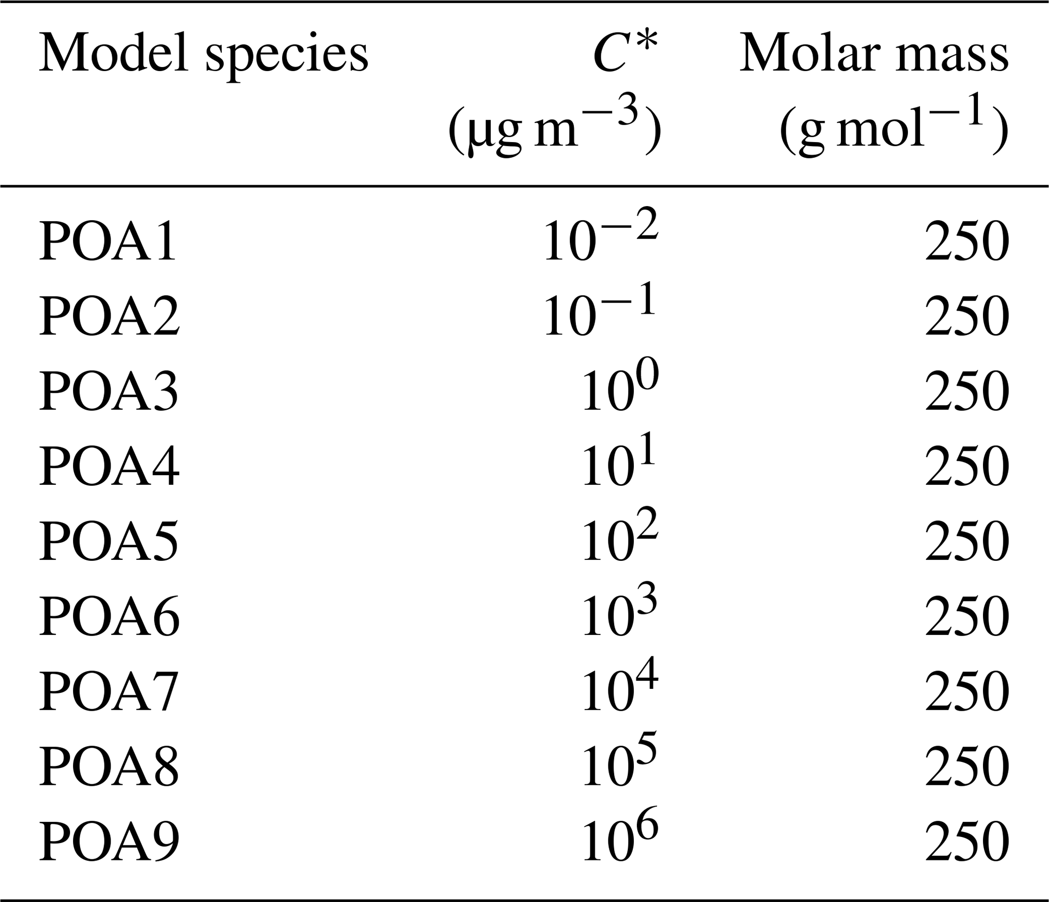
The POA compounds are listed in Table 9.

1. VBS scheme with functionalization process: for carb = 2, the fraction of POA in the gaseous phase can be oxidized by OH radical to form an oxidized POA, noted OPOAx (x represents the bin of volatility defined in Table 9).

2. VBS scheme with functionalization and fragmentation process: for carb = 3, which corresponds to the scheme used in Cholakian et al. (2018). Two processes were added to the VBS scheme presented above. Fragmentation processes, corresponding to the breakup of oxidized OA, compound in the atmosphere into smaller and thus more volatile molecules (Shrivastava et al., 2011) and the formation of non-volatile SOA, where SOA can become non-volatile after forming (Shrivastava et al., 2015).

7.5.2 SOA from VOC oxidation

1. VBS scheme with functionalization process: For soatyp = 6, the formation of SOA from VOC is taken into account with the VBS scheme with functionalization process. Anthropogenic precursors include

   • –

     OLE1: alkenes $k_{\mathrm{OH}}<\mathrm{7}\times {\mathrm{10}}^{\mathrm{4}}$;

   • –

     OLE2: alkenes $k_{\mathrm{OH}}>\mathrm{7}\times {\mathrm{10}}^{\mathrm{3}}$;

   • –

     ALK4: alkanes $\mathrm{5}\times {\mathrm{10}}^{\mathrm{3}}<k_{\mathrm{OH}}<\mathrm{1}\times {\mathrm{10}}^{\mathrm{4}}$;

   • –

     ALK5: alkanes $\mathrm{1}\times {\mathrm{10}}^{\mathrm{4}}<k_{\mathrm{OH}}$;

   • –

     ARO1: aromatics $k_{\mathrm{OH}}<\mathrm{2}\times {\mathrm{10}}^{\mathrm{4}}$;

   • –

     ARO2: aromatics $k_{\mathrm{OH}}>\mathrm{2}\times {\mathrm{10}}^{\mathrm{4}}$.

   SOA yields were kept the same as in the standard VBS scheme described in Zhang et al. (2013); however, instead of using the low-NO_x or the high-NO_x regimes, an interpolation between the yields of these two regimes was added to the model. For this purpose, a parameter is added to the scheme, which calculates the ratio of the reaction rate of RO₂ radicals with NO (high-NO_x regime) with respect to the sum of the reaction rates of the reactions with HO₂ and RO₂ (low-NO_x regime). For this purpose, a parameter (α) was added to the scheme, which calculates the ratio of the reaction rate of RO₂ radicals with NO (ν_NO; high-NO_x regime) with respect to the sum of reaction rates of the reactions with HO₂ (${\mathit{\nu }}_{{\mathrm{HO}}_{\mathrm{2}}}$) and RO₂ (${\mathit{\nu }}_{{\mathrm{RO}}_{\mathrm{2}}}$; low-NO_x regime). The parameter α is expressed as follows:

   $$\begin{array}{}\text{(9)}& \mathit{\alpha }={\displaystyle \frac{{\mathit{\nu }}_{\mathrm{NO}}}{{\mathit{\nu }}_{\mathrm{NO}}+{\mathit{\nu }}_{{\mathrm{HO}}_{\mathrm{2}}}+{\mathit{\nu }}_{{\mathrm{RO}}_{\mathrm{2}}}}}.\end{array}$$

   It represents the part of RO₂ radicals reacting with NO (which leads to applying “high-NO_x yields”). It is calculated for each grid cell by using the instantaneous NO, HO₂, and RO₂ concentrations in the model. Then the following equation is used to calculate an adjusted SOA yield using this α value (Carlton et al., 2009).

   $$\begin{array}{}\text{(10)}& Y=\mathit{\alpha }\times Y_{{\mathrm{highNO}}_x}+(\mathrm{1}-\mathit{\alpha })\times Y_{{\mathrm{lowNO}}_x}\end{array}$$

2. VBS scheme with functionalization and fragmentation process: For soatyp = 7, the formation of SOA from VOC is taken into account with the VBS scheme with the functionalization and fragmentation process. The fragmentation processes for the SVOC start after the third generation of oxidation because fragmentation is favored with respect to functionalization for more oxidized compounds. Therefore, three series of species in different volatility bins were added to present each generation, similar to the approach set up in Shrivastava et al. (2013). For biogenic VOC, fragmentation processes come into effect starting from the first generation, as in Shrivastava et al. (2013), because the intermediate species are considered to be more oxidized. A fragmentation rate of 75 % (with 25 % left for functionalization) is used here for each oxidation step following Shrivastava et al. (2015). The formation of non-volatile SOA is performed by moving a part of each aerosol bin to non-volatile bins with a reaction constant corresponding to a lifetime of 1 h, similar to Shrivastava et al. (2015).

8 Natural emissions

Numerous changes were made in this model version for natural emissions: dimethyl sulfide emissions were added, sea-salt emissions have new parameterizations, mineral dust emissions were improved with mineralogical speciation, and biomass burning can be calculated either with Copernicus Atmosphere Monitoring Service (CAMS) or Analysis and Prediction of the Impact of Fires on Air Quality Modeling (APIFLAME) models and with new vertical profiles; NO_x emissions by lightning were added.

8.1 Dimethyl sulfide emissions

The DMS emissions may now be calculated over the oceans. DMS is a major source of atmospheric sulfur. It contributes to cloud condensation nuclei (CCN) and has thus an impact on cloud formation. DMS atmospheric emission fluxes are parameterized and correspond to a fraction of aqueous DMS sea surface concentrations (nM). These concentrations are extracted from the global database of Lana et al. (2011). The global database contains monthly mean global fields of oceanic DMS with a horizontal resolution of 1^∘ × 1^∘. The aqueous DMS is produced by plankton under light exposure and concentrations are thus sensitive to the time of the year, the latitude, and the sea surface temperature.

In CHIMERE, these monthly mean global fields are projected on the current simulation domain, using land-use information to realistically downscale the values. Using these concentrations, the emitted flux (from ocean to air) is expressed as (Zavarsky et al., 2018)

$$\begin{array}{}\text{(11)}& F=-k\cdot \left({\displaystyle \frac{c_{\mathrm{air}}}{H}}-c_{\mathrm{water}}\right),\end{array}$$

where k (m s⁻¹) is the transfer velocity (also called “piston velocity” in some studies). c_air and c_water are the concentrations of dimethyl sulfide in the air and the water (ocean), respectively, then in gas and liquid phases. H is Henry's law constant and represents the gas solubility, depending on sea salinity and temperature. The most important assumption in the flux calculation is to consider that c_water≫c_air. This is the case in all situations where studies showed that there is at least an order of magnitude between the two. The equation reduces to

$$\begin{array}{}\text{(12)}& F=k\cdot c_{\mathrm{water}}.\end{array}$$

The key point is to estimate k, the transfer velocity. Elliott (2009) studies the dependence of DMS flux on transfer velocity at the global scale. For that, they compare four different emission parameterizations, with several equations for the transfer velocity k_w. These four schemes are implemented in CHIMERE and may be selected using a dedicated user's option. The schemes are Liss and Merlivat (1986), Wanninkhof (1992), Nightingale et al. (2000), and Elliott (2009). The last one is a blend of the first three schemes.

The schemes correspond to best-fit functions built to parameterize the k value. This value depends on the wind speed in the atmosphere (the 10 m wind speed is used here) and the sea surface temperature via the calculation of the DMS Schmidt number. Equations used are those explained in Kettle and Andreae (2000).

After the emission, the DMS reacts chemically in the atmosphere. Chemical reactions were added in the model, both in the MELCHIOR and Statewide Air Pollution Research Center (SAPRC) mechanisms. DMS is oxidized mainly by OH during the day and by NO₃ radicals during the night. It produces SO₂, then sulfate SO${}_{\mathrm{4}}^{\mathrm{2}-}$ (Tesdal et al., 2016). Another pathway of the OH oxidation forms dimethyl sulfoxide (DMSO), intermediate methane sulfinic acid (MSIA), and methane sulfinic acid (MSA) (Chen et al., 2018). The complete chemistry of DMS being extremely complicated, a reduced version is implemented in CHIMERE. The chemical scheme suggested by Mihalopoulos et al. (2007) is used. While aqueous reactions are also available in this scheme, they were not implemented in CHIMERE, since their importance compared to the gas-phase DMS chemistry is small. The final set of added reactions is

$$\begin{array}{}\text{(13)}& \left\{\begin{array}{lll}\mathrm{DMS}+\mathrm{OH}& \to & \mathrm{0.997}({\mathrm{SO}}_{\mathrm{2}}+{\mathrm{CH}}_{\mathrm{3}}{\mathrm{O}}_{\mathrm{2}}+\mathrm{HCHO})\\ & +& \mathrm{0.003}(\mathrm{MSA}+\mathrm{HCHO})\\ \mathrm{DMS}+\mathrm{OH}& \to & \mathrm{DMSO}\\ \mathrm{DMS}+{\mathrm{NO}}_{\mathrm{3}}& \to & {\mathrm{SO}}_{\mathrm{2}}+{\mathrm{HNO}}_{\mathrm{3}}+{\mathrm{CH}}_{\mathrm{3}}{\mathrm{O}}_{\mathrm{2}}+\mathrm{HCHO}\\ \mathrm{DMSO}+\mathrm{OH}& \to & \mathrm{MSIA}+{\mathrm{CH}}_{\mathrm{3}}{\mathrm{O}}_{\mathrm{2}}\\ \mathrm{MSIA}+\mathrm{OH}& \to & {\mathrm{CH}}_{\mathrm{3}}{\mathrm{O}}_{\mathrm{2}}+{\mathrm{SO}}_{\mathrm{2}}+{\mathrm{H}}_{\mathrm{2}}\mathrm{O}.\end{array}\right.\end{array}$$

8.2 Sea-salt

In the previous CHIMERE versions, the only way to calculate the sea-salt emissions was the Monahan (1986) parameterization. There was also two flags for the sea-salt management in the chimere.par parameter file. In this model version, there is now only one flag, iusesalt, and four schemes for the sea-salt emissions calculations. Other improvements are (i) the sea-salt calculations are now able to take into account the difference between inland water and lakes, (ii) the sea ice is removed from the sea surface estimation for the calculation. The modeled species are NA for the sodium fraction, HCl, the chloride fraction, H₂SO₄, the sulfate fraction, and WATER, the water fraction. The interest to split the sea-salt chemical contribution is to have access to Na and Cl concentrations, later used in the model to more precisely calculate the pH.

The Monahan (1986) parameterization can be used setting iusesalt = 1 and calculates emission fluxes as

$$\begin{array}{}\text{(14)}& {\displaystyle \frac{\mathrm{d}F}{\mathrm{d}r}}={\displaystyle \frac{\mathrm{1.373}\times U_{\mathrm{10}}^{\mathrm{3.41}}}{r^{\mathrm{3}}}}\left(\mathrm{1}+\mathrm{0.057}{r}^{\mathrm{1.05}}\right){\mathrm{10}}^{\mathrm{1.19}{e}^{-B^{\mathrm{2}}}}\text{(15)}& {\displaystyle }\mathrm{where}B={\displaystyle \frac{\mathrm{0.38}-\log \left(r\right)}{\mathrm{0.65}}}.\end{array}$$

F is the flux of sea-salt particle number in particles m⁻² s⁻¹ µm⁻¹, r is the particle radius (µm), and U₁₀ is the 10 m wind speed (m s⁻¹). The sea-salt flux is calculated with several limitations: only for 10 m wind speed less than or equal to 30 m s⁻¹ and with a fixed size distribution. This scheme is for the indirect mechanism (bubble bursting) and not the direct mechanism (spume) as explained by Grini et al. (2002). For the direct mechanism, the parameterization proposed by Monahan (1986) was found to produce too much and is thus not implemented in our case. This scheme is designed to be used for particles bigger than 0.8 µm but is used for all sizes in many models, such as in CHIMERE's previous version. In order to have an alternative method for small size particles, two additional schemes are implemented: the Martensson et al. (2003) and Grythe et al. (2014) schemes. In addition, a mix is possible between Monahan (1986) and Martensson et al. (2003) for the size distribution. This mix can be selected by the user by using iusesalt = 2. In this case, the flux is calculated using Monahan (1986), but the way to distribute this flux into the aerosol size distribution is calculated after Martensson et al. (2003).

The scheme of Martensson et al. (2003) is available with iusesalt = 3. This scheme is designed for an aerosol mean mass median diameter of until D_p=2.8 µm. Up to D_p=2.8 µm, the mass flux is estimated using Monahan (1986). The interest of this scheme is that the size distribution is temperature dependent. This scheme makes also the differences between the dry and wet radius of the particle for the calculation.

The same temperature influence is taken into account with the scheme of Grythe et al. (2014) using iusesalt = 4. The flux is calculated as

$$\begin{array}{lll}\frac{\mathrm{d}F(D_{\mathrm{p}},U_{\mathrm{10}},T)}{\mathrm{d}{D}_{\mathrm{p}}}& =& T_{\mathrm{w}}\cdot \left[\mathrm{235}\cdot U_{\mathrm{10}}^{\mathrm{3.5}}\exp \left(-\mathrm{0.55}{\left[\ln \left(\frac{D_{\mathrm{p}}}{\mathrm{0.1}}\right)\right]}^{\mathrm{2}}\right)\right.\\ & +& \mathrm{0.2}{U}_{\mathrm{10}}^{\mathrm{3.5}}\exp \left(-\mathrm{1.5}{\left[\ln \left(\frac{D_{\mathrm{p}}}{\mathrm{2}}\right)\right]}^{\mathrm{2}}\right)\\ & +& \left.\mathrm{6.8}{U}_{\mathrm{10}}^{\mathrm{3.0}}\exp \left(-\mathrm{1.0}{\left[\ln \left(\frac{D_{\mathrm{p}}}{\mathrm{30}}\right)\right]}^{\mathrm{2}}\right)\right],\end{array}$$

with T_w (K) as the temperature dependence of production at temperature T, the sea surface temperature, and is estimated as

$$\begin{array}{}\text{(16)}& T_{\mathrm{w}}\left(T\right)=\mathrm{0.3}+\mathrm{0.1}T-\mathrm{0.0076}{T}^{\mathrm{2}}+\mathrm{0.00021}{T}^{\mathrm{3}}.\end{array}$$

8.3 Mineral dust

The mineral dust emissions calculation remains highly uncertain in transport models (Cuevas et al., 2015; Middleton, 2017). This uncertainty is linked to the fact that these emissions are estimated based on a threshold process computed with very uncertain forcings (Alfaro and Gomes, 2001; Darmenova et al., 2009). The emission measurements are rare and, when they exist, representative mainly of a very local environment (a few tens of meters around the measurement site) (Kok et al., 2012). In CHIMERE v2020r1, several improvements were done on the mineral dust emissions flux calculation: (i) implementation of several subgrid-scale approaches to take into account soil and surfaces variabilities, and (ii) the mineralogy to explicitly model several species instead of only one.

8.3.1 Subgrid-scale variability

The problem of using a threshold is that the transition between a zero and a non-zero value is very sensitive to the accuracy of the forcing parameter and on its spatial and temporal representativity. For the mineral dust emissions calculation, the key parameters are the 10 m wind speed and the surface and soil type, including the eolian roughness length (Shao, 2001; Engelstaedter et al., 2006). Their spatial representativity is the one of the model cell and may be different than the local phenomenon to model.

The best way to represent such processes is to calculate distributions: the input parameters are not used with a single value, which has high uncertainty, but with their distribution. This distribution represents at the same time the uncertainty and the spatiotemporal variability around the mean averaged value.

For the 10 m wind speed, the subgrid-scale variability was first represented using a Weibull distribution (Menut, 2008). The Weibull k shape parameter was constant and equal to k=4. It was shown that the emissions were very sensitive to a change of the k value. In fact, there is no reason for the k parameter to be constant. Its value could depend on many parameters to express the surface and soil variability in the modeled cell. In Menut (2018), the k parameter is linked to the subgrid-scale variability of the orography. The differences in emissions are quantified over Africa: the correlation is slightly improved but the RMSE, compared to AERONET AOD data, is well decreased. The use of the k parameter variability is a user's option.

For soil and surface properties, a subgrid-scale variability was also implemented. In general, global, and regional models use the dominant land-use and soil properties in their domain cells. For each cell, there is one characteristic and the emissions flux is thus calculated once. Using high-resolution (30 s) United States Geological Survey (USGS) databases, we implemented a matrix, providing for each model cell the percentage of each soil type, and for each one, the percentage of each land-use type. The USGS database has 16 soil categories and 24 land-use categories; the dust flux is calculated for a maximum of 384 combinations. The values are then accumulated to have the mean flux in the cell.

8.3.2 Mineralogy

Among many others, one interest of the mineral dust modeling is to calculate accurate aerosol deposition fluxes (Sokolik and Toon, 1999). For biogeochemical studies, the deposition of mineral dust over the ocean is of interest, in particular for phytoplankton growth (Zhang et al., 2015). In this new model version, the detailed mineralogy of dust was implemented, following the development of Balkanski et al. (2007). Instead of one mineral dust species called “dust”, 12 mineral species are emitted, transported, and deposited. They are calcite, chlorite, feldspar, goethite, gypsum, hematite, illite, kaolinite, mica, quartz, smectite, and vermiculite (Claquin et al., 1999; Balkanski et al., 2007). Each one has a specific density, silt/clay ratio, and refractive index. As with the mean mineral dust, these species are described with a binned size distribution (in general, 10 bins, as recommended in the parameter file). The complete parameterization and results are presented in Menut et al. (2020b). The use of this mineralogy may be numerically expensive due to the larger number of emitted species (12), which are then transported and deposited. This doubles the number of aerosols in the CHIMERE model.

8.4 Forests biomass burning emissions

Forests biomass burning emission fluxes may be included in CHIMERE model simulations using two different sources:

• The CAMS model fluxes with a horizontal resolution of 0.1 × 0.1^∘. These fluxes are reprojected on the CHIMERE grid and with the used chemical model species.

• The APIFLAME model fluxes, with an adaptable horizontal resolution, up to the maximum resolution of 1 km × 1 km. This model reads satellite data, global model fuel load, and calculates emission fluxes. This model is more dedicated to research and enables development of new biomass burning parameterizations, development scenarios, the ability to change the hypothesis on the emitted chemical species, etc.

8.4.1 The CAMS pre-processor

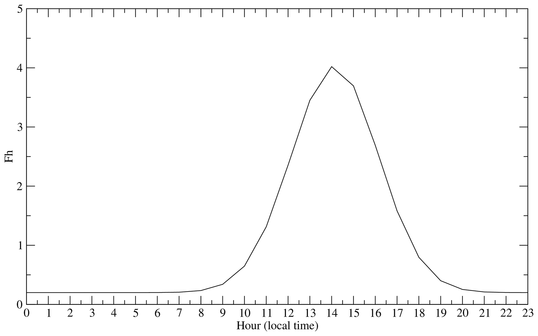
The pre-processor for ECMWF CAMS data formatting is a program distributed with the new CHIMERE version. The goal is to download the ECMWF model outputs of Kaiser et al. (2012) and adapt them to the CHIMERE format. For this formatting, several conversions are needed: projecting the data onto the CHIMERE simulation grid, converting the proposed chemical model species to the CHIMERE chemical mechanism species, and temporally refining the data by shifting the time resolution from daily to hourly fluxes. All available chemical species are downloaded and used to create the CHIMERE emitted species. Temporally, having no realistic information to move from daily to hourly emissions fluxes, an academic diurnal profile is applied to the daily data as

$$\begin{array}{}\text{(17)}& \begin{array}{lll}{F}_{\mathrm{h}}& =& d_{\mathrm{w}}+(\mathrm{1}-d_{\mathrm{w}})\frac{\mathrm{24}}{d_{\mathrm{s}}\sqrt{\mathrm{2}\mathit{\pi }}}\\ & \times & \exp \left(-\mathrm{0.5}{\left(\frac{h+\mathrm{0.5}+\mathit{\delta }-t_{\mathrm{0}}}{\mathrm{2}{d}_{\mathrm{s}}}\right)}^{\mathrm{2}}\right),\end{array}\end{array}$$

with the constant values of h, the current GMT hour, d_w=0.2, d_s=2.0, t₀=13.5, and δ= longitude/360 × 24. An example is displayed in Fig. 11.

Figure 11 Academic hourly profile applied to the constant daily wildfire fluxes.

8.4.2 APIFLAME v2

APIFLAME was designed to calculate the emissions from biomass burning at high spatial and temporal resolution with flexibility in terms of the input data used. While the CAMS approach is based on fire radiative power (FRP) detection (active fires), APIFLAME calculates emissions based on the burned area and resulting biomass consumed (in terms of carbon), as described in Menut et al. (2013) and Turquety et al. (2014). Maps of the burned areas and FRP on the user-defined grid are derived (with the corresponding geog file) from MODIS satellite observations (MOD14 and MCD64A1, respectively, version v006), combined with the information on the vegetation type (satellite observations or land-use databases). Depending on the type of vegetation burned, the amount of carbon consumed is calculated by multiplying the burned area with the fuel consumption derived from the Organising Carbon and Hydrology In Dynamic Ecosystems (ORCHIDEE) land surface model (Turquety et al., 2014). Emissions for inventory species are then calculated using a list of emission factors and converted to emission fluxes for CHIMERE species using aggregation matrices accounting for the reactivity to OH (either the SAPRC or MELCHIOR chemical scheme).

The main improvement included in version 2 (Turquety et al., 2020) is related to temporal variability, with the possibility to (i) redistribute the total monthly burned area (MCD64 data) according to the FRP value (MOD14 data) so that higher emissions will correspond to enhanced fire intensity; (ii) redistribute daily emissions using the diurnal variability of the FRP in the geostationary observations (Spinning Enhanced Visible and Infrared Imager (SEVIRI) above Europe and Africa). Small fires that may be observed with the active fire detection (FRP), but are not present in the burned area product, may also be included.

The flexibility of the use of input datasets for fire activity or vegetation type burned allows for the calculation models in an ensemble that provide information on the uncertainties related to these choices. The analysis of a case study in Portugal during the summer of 2016 shows an average dispersion of ∼ 75  % of daily carbon emissions. The list of species included may also be modified without modifying the core of the model (input datasets).

8.4.3 The height and shape of the vertical injection

The CAMS or APIFLAME data provide a biomass burning surface flux. It is necessary to vertically redistribute the flux along a profile representing pyroconvection. The injection height, H_p, estimation is based on the Sofiev et al. (2012) scheme, as

$$\begin{array}{}\text{(18)}& H_{\mathrm{p}}=\mathit{\alpha }{H}_{\mathrm{abl}}+\mathit{\beta }{\left({\displaystyle \frac{\mathrm{FRP}}{P_{f\mathrm{0}}}}\right)}^{\mathit{\gamma }}\exp \left(-\mathit{\delta }{N}_{\mathrm{FT}}^{\mathrm{2}}/N_{\mathrm{0}}^{\mathrm{2}}\right),\end{array}$$

with α=0.24, β=170 m, γ=0.35, and δ=0.6, P_f0=10⁶ W, and $N_{\mathrm{0}}^{\mathrm{2}}=\mathrm{2.5}$ × 10⁻⁴ s⁻². N_FT is the Brunt–Väisälä frequency and is calculated between H_abl and the pressure level corresponding to 300 hPa (to ensure it remains in the free troposphere). The FRP is expressed in watts and is provided by the emission flux data. In the case of “huge” fires, i.e., if the H_p value is greater than 1500 m a.g.l., the calculation is redone following Veira et al. (2015), after replacing FRP with FRP^* =$\mathrm{FRP}\sqrt{H_{\mathrm{p}}/H_{\mathrm{deep}}}$, with H_deep = 1500 m.

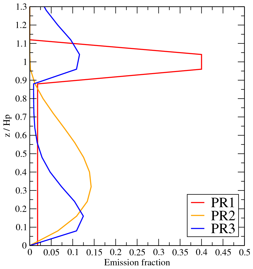
Figure 12 Vertical profiles of factors used for the vertical redistribution of the biomass burning emissions fluxes.

After the estimation of the height of the mass injection, it is possible to estimate the shape of the injection profile. Three user options have been implemented in the model (Fig. 12).

• PR1: the mass flux is separated into two parts: 20 % is injected between the surface and 0.9×H_p and 80 % between 0.9×H_p and 1.1×H_p. Inside these two intervals, the flux is constant with altitude. This profile is close to the shape of the convective profile obtained using thermal parameterizations.

• PR2: the emissions are injected between the surface and H_p, following a profile close to the one used in Veira et al. (2015) with a K_z-like shape:

  $$\begin{array}{}\text{(19)}& \left\{\begin{array}{ll}\mathrm{if}{z}_n\le \mathrm{1}& \mathrm{EF}\left(z\right)=H_{\mathrm{p}}{z}_n{\left(\mathrm{1}-z_n\right)}^{\mathrm{2}}\\ \mathrm{if}{z}_n>\mathrm{1}& \mathrm{EF}\left(z\right)=\mathrm{0}.\end{array}\right.\end{array}$$

  with EF as the emission flux and $z_n=z/H_{\mathrm{p}}$.

• PR3: this profile also uses a K_z-like shape but with two maxima: one in the surface layer and one around H_p.

These profiles were tested in Menut et al. (2018), with the simulation of biomass burning episodes in the center of Africa. It was shown that, after long-range transport, the atmospheric concentration of pollutants is not very sensitive to the shape of the vertical profile. It is mainly due to the fact that pyroconvection has higher temperature and more turbulence than the environment: the emitted species are quickly and homogeneously mixed in the whole column between the surface and H_p.

8.5 NO_x by lightning

The emissions of NO_x from lightning were added in this version. These emissions occur in the case of deep convection and convective precipitation. The detailed implementation and its impact on chemical concentration is explained in Menut et al. (2020a). The scheme implemented is simple and follows the Price and Rind (1993) scheme, based on the presence and vertical structure of convective clouds. The use of this parameterization is more realistic, in particular at tropical latitudes, when lightning flashes are the most often observed. These emissions improve the aerosol optical depth in Africa but have limited impact on the surface concentrations of pollutants in Europe.

9 Impact of several changes in the model

The previous sections presented all the changes made in this model version. For some of these changes, simulations were carried out in order to examine their impact. Note that compared to Sect. 3, the reference simulation was done here with WRF forced by NCEP global meteorological fields.

The following sensitivity tests were performed:

• “ref” is the reference simulation. The following simulations are done by changing one (and only one) parameter of this simulation.

• “BCclim”: in place of the daily boundary conditions from CAMS, we use the climatological boundary conditions, distributed with the model and performed using the Goddard Chemistry Aerosol Radiation and Transport (GOCART) and LMDz-INCA global models.

• “nofire”: biomass burning emissions were set to zero in place of the CAMS emissions in “ref”.

• “wesely”: this simulation used the Wesely (1989) scheme for dry deposition in place of the Zhang et al. (2001) scheme in “ref”.

• “despres”: this simulation used the Després and Lagoutière (1999) transport scheme for vertical advection in place of the Van Leer (1977) in “ref”.

• “HTAP”: this simulation used Hemispheric Transport of Air Pollution (HTAP) anthropogenic emissions in place of the EMEP emissions.

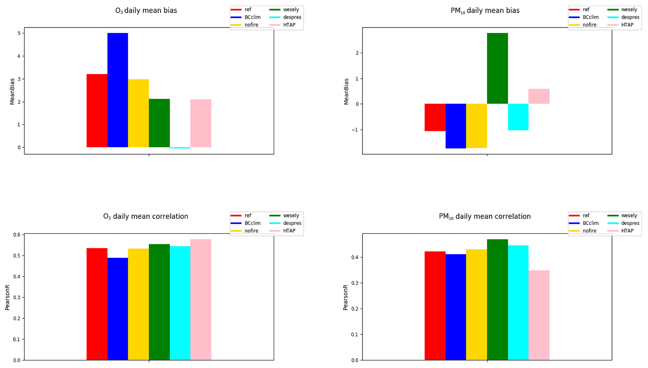
Figure 13 Bias (µg m⁻³) and correlation ($-\mathrm{1}:\mathrm{1}$) for O₃ and PM₁₀ surface concentrations for several sensitivity tests.

Results are presented in Fig. 13, with the daily mean bias (in µg m⁻³) and correlation (between −1 and 1) for surface ozone and PM₁₀ concentrations. For ozone, the reference case shows a mean daily bias of +3.29 µg m⁻³. By changing the boundary conditions, this bias increased to +4.81 µg m⁻³. The choice to not use biomass burning emissions reduced this bias to 3.10 µg m⁻³. It means that the addition of fires emissions does not have a large mean impact on the ozone surface concentrations. But this is normal, as fires events, even if they may induce a large increase in ozone concentrations, are only present for a few days during a year. The change of the dry deposition scheme has a large impact for ozone, decreasing the bias a lot to 2.35 µg m⁻³. The largest impact on ozone bias was from the new vertical transport scheme of Després and Lagoutière (1999): the bias was reduced to −0.05 µg m⁻³. Finally, the change of the anthropogenic emissions inventory, by using HTAP in place of CAMS, also has an impact, with a decreased bias of 1.48 µg m⁻³.

For PM₁₀, the bias also changed a lot, depending on the used parameterization. With the reference case, the bias was −1.42 µg m⁻³. The bias became larger and was always negative for the change in boundary conditions and when not taking into account biomass burning, with biases of −2.12 and −1.87 µg m⁻³, respectively. The most important change was the bias becoming positive (+2.89 µg m⁻³) with the dry deposition scheme of Wesely (1989). For the use of the vertical transport scheme of Després and Lagoutière (1999), the bias remained negative but was reduced to −0.92 µg m⁻³. Finally, in another positive case, was the change of the emissions inventory, with a bias of +0.43 µg m⁻³ with the use of HTAP. For the correlation, for ozone and PM₁₀, the changes were not as large as the biases. For ozone, the values were between 0.51 and 0.60 µg m⁻³, when the reference was 0.56 µg m⁻³, and, for PM₁₀, the values were between 0.34 and 0.48 µg m⁻³, when the reference was 0.43 µg m⁻³. For several cases, some compensation errors were possible, but, it was noticeable that the use of the new vertical transport scheme of Després and Lagoutière (1999) was the only case where scores were improved for all pollutants. Reduction on the positive ozone bias close to the ground could be linked to the antidiffusive properties of the Després and Lagoutière (1999) scheme, reducing erroneous downward transport of ozone from the higher troposphere which has been shown by, e.g., Emery et al. (2011), to be a major source of overestimation of ozone concentration in the midlatitudes. Implementation of the Després and Lagoutière (1999) scheme in CHIMERE is discussed in detail in Lachatre et al. (2020), which shows the strong reduction in vertical diffusion obtain with the use of this scheme relative to Van Leer (1977). Mailler et al. (2021) discusses in more detail the strengths and weaknesses of this scheme relative to Van Leer (1977).

10 Model's time integration

The model's time integration benefits from two main changes for this new version: (i) the three time steps were optimized and the adaptive time step is more efficient and robust; (ii) the process integration may now be done with the original approach of “production/loss budget” or through using the newly implemented approach of “operator splitting”.

10.1 Time management

The time management in the model was already defined in Menut et al. (2013). In this model version, some changes were done, mainly due to the need to manage variable time steps with the online version. Three time steps are defined: the hour, a physical time step called dtphys, and a chemical time step called dtchem.

The hour is obviously a fixed time step of 1 h. This interval is mandatory since many input model data are provided at an hourly frequency: meteorological fields, emissions, and boundary conditions, for example. It is also the frequency used to read the data in offline mode.

The physical time step dtphys is defined by the user in the CHIMERE parameter file. In offline mode, it indicates the value that the user wants for the transport calculation. The meteorological data are linearly interpolated between 2 consecutive hours; therefore, the number of steps may change the simulated chemical concentrations in the case of a rapid change in meteorology from one hour to the next. In online mode, this time step has another meaning and represents the exchange frequency of variables between WRF and CHIMERE.

The chemical time step dtchem is also defined in the CHIMERE parameter file. But, in this case, it is just a recommendation. The CFL is calculated in each cell and at each time step and if a lower dtphys value is necessary, the calculated value is used. The dtphys value is estimated as

$$\begin{array}{}\text{(20)}& \mathrm{\Delta }t={\displaystyle \frac{{\mathrm{CFL}}_{\max }\times \mathrm{\Delta }x}{U}},\end{array}$$

where CFL_max is the maximum acceptable CFL value. Theoretically, CFL_max=1, but to avoid numerical instabilities during the transport, CFL_max=0.8 is recommended. If the user experiences instabilities, it is possible to reduce this value in the parameter file. Δx is the grid-cell width (m) and U is the wind speed (m s⁻¹). The value of Δt is calculated for U, with the zonal wind component, u, the meridian wind component, v, the vertical wind component, w, and the deep convection components (updraft and downdraft). The minimum of all these values is retained as the necessary time step. In general, it is the w value which limits the time step. This calculation is performed for each subdomain of the parallelized domain and the minimum value is retained. Finally, an adjustment is done to ensure that dtphys is an exact multiple of dtchem. As the CFL calculation is performed every dtphys, it is possible to have a different dtchem value at each physical time step. This adaptive time step was shown to be very efficient at decreasing the computational time of a simulation.

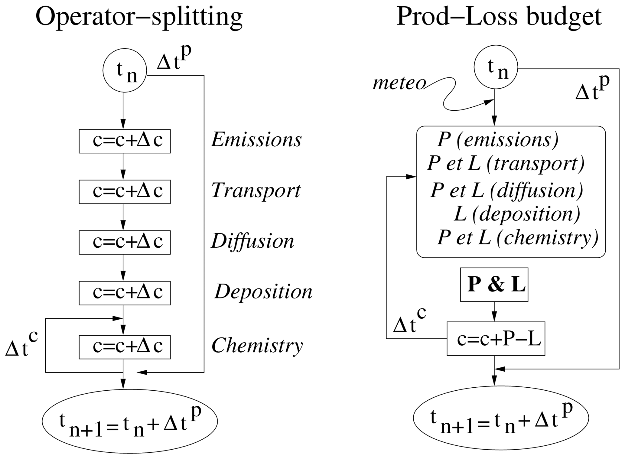
Figure 14 Principle of the time integration in the model of all processes calculated to update the chemical concentration fields.

10.2 Operator splitting

The integration of all processes to update the concentrations in a chemistry-transport model is a well-known problem and several methods exist. Until the 2017 version, the update in time of the chemical concentrations was done using the production/loss approach, as presented in Fig. 14. In this case, all production (P) and loss (L) terms are calculated independently. The update of a chemical concentration is thus done by integrating the following equation:

$$\begin{array}{}\text{(21)}& {\displaystyle \frac{\partial c}{\partial t}}=P-L\cdot c.\end{array}$$

All production and loss terms are calculated at the same time and integrated all together. To solve this complex system, the numerical method used is the two-step algorithm developed by Verwer (1994). It consists of a Gauss–Seidel scheme to have a stable update of all concentrations, whatever their lifetime. Its strength is that there is no splitting error, linked to the order of the processes. Its weakness is that the time step required is constrained to the smallest time step, which is, general, the time step required for the chemical modeling. This means that many of the concentrations are updated for the transport and the mixing much more often than necessary. The results are more accurate but slower to obtain than with the splitting method.

In this version, the operator-splitting approach was added. It is a well-known approach, widely used in chemistry-transport models (McRae et al., 1982). Contrary to the two-step approach, the chemical concentration is updated with each process one by one. A new concentration is thus calculated with the transport, then with the mixing, then with the chemical reactions, etc. Its strength is that the time step used may be different between each process: knowing that the chemical reactions need a fast time step, it is possible to update the chemistry with a small time step, and to later update the concentrations with the transport, which uses a larger time step. Globally, this speeds up the model integration. But its weakness is that the results depends on the order of the processes. The results are less accurate but obtained faster than with the prod/loss approach. Finally, knowing the strengths and weaknesses, the user can select their own approach, with, for example, the production/loss approach for analysis and the operator-splitting approach for forecasting.

Figure 15 Principle of the nesting in the case of offline or online coupling.

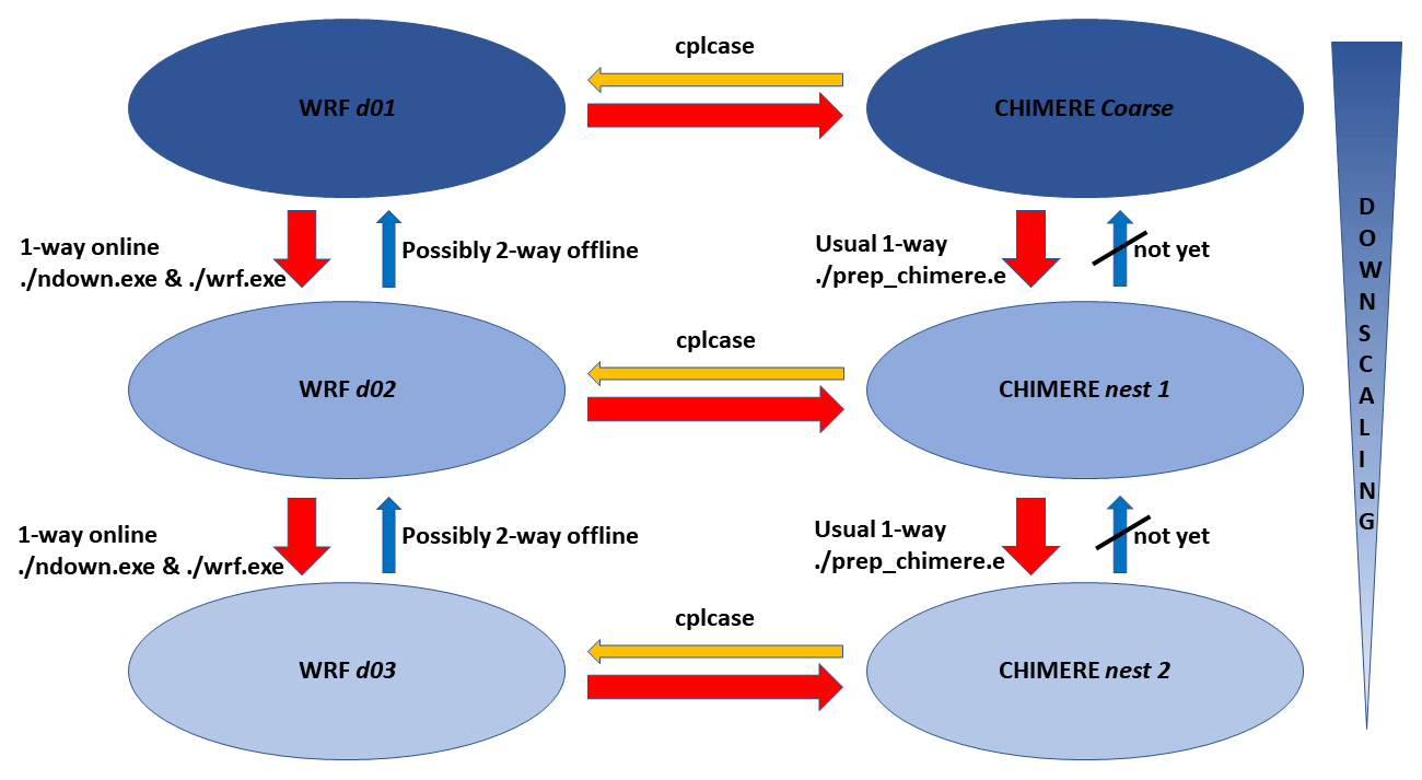
10.3 Flexibility on outputs

The output files may be very large, depending on the grid size and the simulation duration. More flexibility was added in this model version to have less variables in the output files if the user is interested in basic output variables only. This may be convenient for forecasting users, for example, where only tracked pollutants are used and not all defined variables in the model.

For the output concentration species, there is no change in this version. The difference between the low and full flags are whether to write the aerosols bin per bin or not. In all cases, the total mass of each aerosol species is written. For the deposition, the novelty is that by selecting nsdepos = 0, the output file for dry and wet deposition is not created. This is a gain in runtime and disk space if the user is not interested in analyzing the deposition fluxes. For the meteorology, a new flag called accurmet is added in the parameter file, with three different possible values: low, medium, and full. With accurmet = low, only the two-dimensional meteorological fields are written in the output: the 2 m temperature and 2 m relative humidity, the 10 m wind speed, and the boundary layer height. With accurmet = medium, the previous fields are written, with, in addition, the three-dimensional fields of pressure, temperature, specific humidity, and wind components u and v. Finally, with accurmet = full, all meteorological fields treated by the model are written in output. This includes deep convection mass fluxes, ice, snow, and rain.

Figure 16 Time to solution of WRF and CHIMERE in minutes per simulated day as a function of computational resources for cpl_case = 1 (a) and cpl_case = 4 (b).

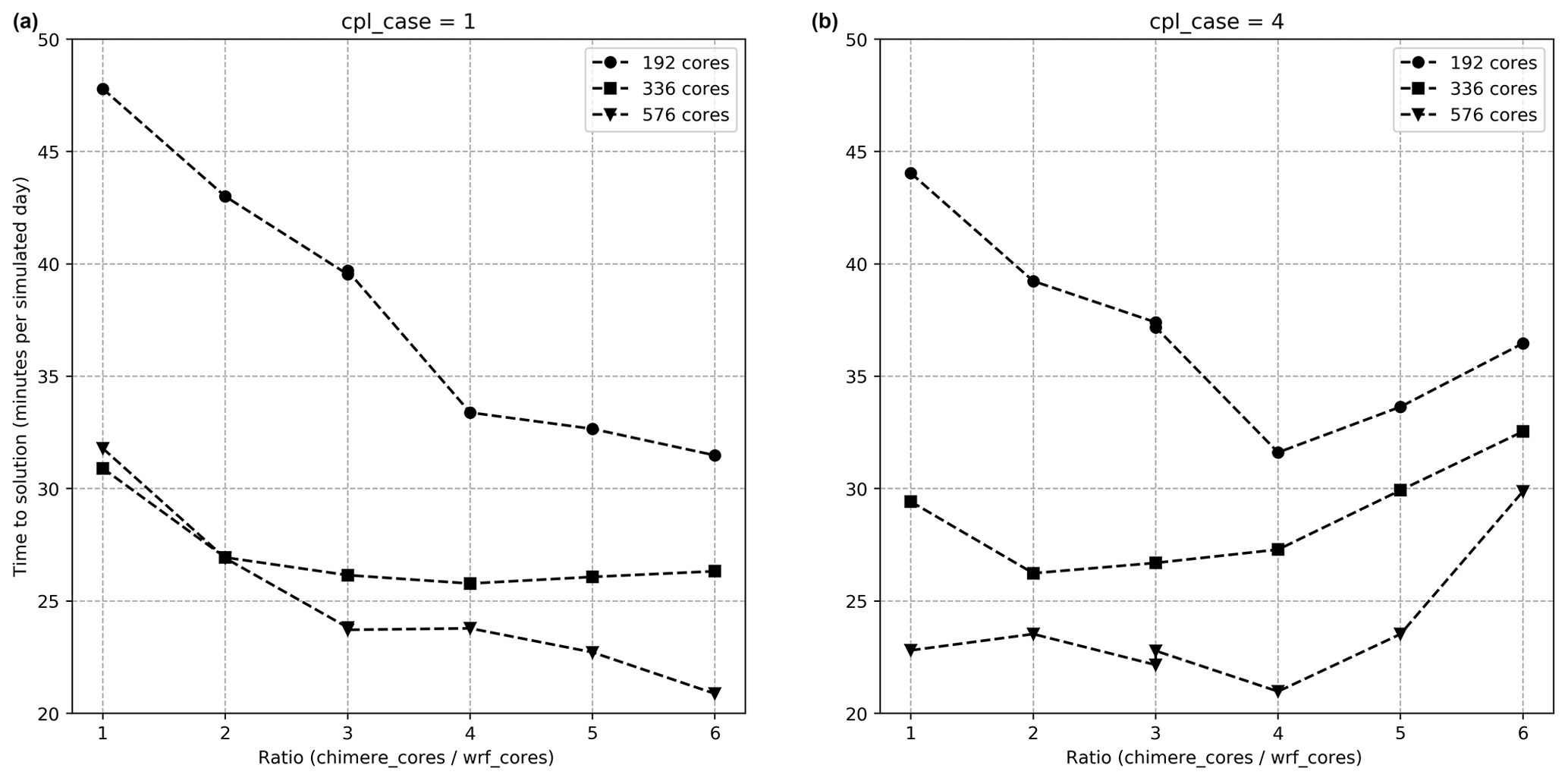
Figure 17 Time to solution for the coupled model in minutes per simulated day as a function of the ratio of CHIMERE cores to WRF cores for 192, 336, and 576 total number of cores. and for cpl_case = 1 (a) and cpl_case = 4 (b).

11 Nesting and nudging

For the nesting, the method of how it is managed with this new version is presented in Fig. 15. As with the previous version, CHIMERE authorizes nesting up to three levels. However, the namelist files can be easily changed to increase the depth of the nesting.

In offline mode, CHIMERE can be used as usual with meteorological forcing through WRF, ECMWF, or from other sources of data. In this case, WRF can be run in one-way or two-way nesting; then CHIMERE is run after, as usual, for each domain with one-way nesting. If the online flag is activated (online = 1), the model is fully coupled with WRF, with different complexities of coupling (cpl_case flag). For this case, two-way nesting is not permitted, each level of nesting is run, WRF and CHIMERE exchange information frequently but there is no online feedback to the level above to update both the species concentrations and meteorological fields. To achieve this one-way nesting procedure, the ndown.exe WRF executable is used, permitting the use of meteorological outputs coming from the above domain to drive the nested domain. Therefore, for a given level of nesting, WRF and CHIMERE are always run using the downscaled information from the level above and never benefiting from the interior level, if it exists. A nested domain can use different numbers of vertical levels, as long as the top height of the nested domain is less than the top height of the parent domain.

For the nudging, the CHIMERE-WRF coupled suite can use the WRF nudging option to avoid strong divergences inside the models. This used in coarse model simulations (typically above 25 km resolution) that are driven by global-scale simulations, commonly issued from Global Forecast System (GFS) or ECMWF datasets that have been re-analyzed with synoptic observations. At higher resolutions with nested domains, model nudging should be not necessary to allow the model to accurately develop the local physics and dynamics. For the chemistry, model nudging is not used, but the assimilation of observation data (from satellite and ground stations) is an area of interest that is not yet fully operational in this version of CHIMERE.

12 Computing performance

Computing performance and scalability are studied with a series of 1 d long run performed on the Irene Joliot-Curie machine of Très Grand Centre de Calcul (TGCC) with a varying number of cores dedicated to WRF and CHIMERE for coupling cases (cpl_case) 1 and 4. To increase the number of points and therefore allow the use of more cores, the MED20 domain (same domain as MED60 but at 20 km horizontal resolution) is used. The effective computational times spent in both components of the coupled system (WRF and CHIMERE) are obtained with the LUCIA tool of the OASIS3-MCT coupler (Maisonnave and Caubel, 2014) which enables separation of computational time and waiting time. The scalability is presented in Fig. 16 using a time to solution (in minutes per simulated day) criteria omitting any waiting time due to load imbalance between the two components. In both coupling cases, the CHIMERE behavior remains the same with a good scalability up to 200 hundred cores. WRF behavior differs in cpl_case 4 when direct and indirect aerosol effects are at stake due to specific calculations in this case; however, scalability remains correct up to 100 cores. In both cases, WRF is faster than CHIMERE; therefore, the speed of CHIMERE is key in the overall performance of the coupled model.

The time to solution of the coupled model as a whole is presented in Fig. 17 as a function of the ratio of cores attributed to CHIMERE to the cores attributed to WRF for three different constant total number of cores. Essentially for cpl_case 1, the more cores that are given to CHIMERE, the better the performance is, especially if the total number of cores is relatively small. For the cpl_case 4, the core balancing between the two models is more important for performance. If the number of cores given to WRF becomes too small, the performance decreases. In this particular experiment, a ratio between 2 and 4 seems to be optimal.

Those results show computational time for both components, but in a coupled framework, they do not infer scalability when used in standalone mode. Moreover, scalability and performance are strongly dependent on the machine and the size of the domain. Custom sensitivity analysis on each setup is always better, but as a rule of thumb a ratio of 2 to 4 CHIMERE cores to 1 WRF core is recommended for good performance.

13 Conclusions

This article presented the new CHIMERE chemistry-transport model version. All new commands and parameterizations were extensively described. This version is an important step forward compared to evolutions of the previous versions. First, this is the first online coupled version, in this case with the WRF meteorological model. It enables to model the direct and indirect effects of aerosols on meteorology. The validation of this version was performed using surface measurements of pollutant concentrations, aerosol optical depth, and vertical ozone soundings. Statistical scores were calculated including bias, correlation, and RMSE, as well as scores on ozone daily maximum concentrations being of importance for users making forecasts. A long-term simulation showed this new feature does not drastically change the results for pollutants at a large scale. But for high-resolution studies, this process has an increasing importance. Second, all natural emissions were revised and updated: mineral dust, sea salt, and biomass burning. The NO_x emissions by lightning were also added. Third, the aerosol chemistry was also improved with the addition of the VBS and H²O schemes. Fourth, the subgrid-scale variability of concentrations due to emissions by activity sectors is also now included in this version. Finally, a new vertical advection scheme was added, which has been shown to strongly reduce excess vertical diffusion. Compared to the previous model version, this new one has the same performance for the correlation of ozone, but the bias has been improved. For forecasting, the daily maxima are also better modeled. For aerosols and optical depth, the results are much better with v2020r1 for both the correlation and bias.