Iodine chemistry in the chemistry–climate model SOCOL-AERv2-I

In this paper, we present a new version of the chemistry–climate model SOCOL-AERv2 supplemented by an iodine chemistry module. We perform three 20-year ensemble experiments to assess the validity of the modeled iodine and to quantify the effects of iodine on ozone. The iodine distributions obtained with SOCOL-AERv2-I agree well with AMAX-DOAS observations and with CAM-chem model simulations. For the present-day atmosphere, the model suggests that the iodine-induced chemistry leads to a 3 %–4 % reduction in the ozone column, which is greatest at high latitudes. The model indicates the strongest influence of iodine in the lower stratosphere with 30 ppbv less ozone at low latitudes and up to 100 ppbv less at high latitudes. In the troposphere, the account of the iodine chemistry reduces the tropospheric ozone concentration by 5 %–10 % depending on geographical location. In the lower troposphere, 75 % of the modeled ozone reduction originates from inorganic sources of iodine, 25 % from organic sources of iodine. At 50 hPa, the results show that the impacts of iodine from both sources are comparable. Finally, we determine the sensitivity of ozone to iodine by applying a 2-fold increase in iodine emissions, as it might be representative for iodine by the end of this century. This reduces the ozone column globally by an additional 1.5 %–2.5 %. Our results demonstrate the sensitivity of atmospheric ozone to iodine chemistry for present and future conditions, but uncertainties remain high due to the paucity of observational data of iodine species.

1 Introduction

Emissions of chlorine- and bromine-containing halogen compounds have long been the subject of scientific investigation because they play an important role in the catalytic destruction cycles of stratospheric ozone (Solomon, 1999). Recent studies demonstrate the success of the Montreal Protocol and its amendments in phasing out the emissions of chlorine- and bromine-containing substances and also point to early signs of stratospheric ozone recovery (e.g., Newman et al., 2009; Egorova et al., 2013; WMO, 2018). At the same time, our understanding of iodine-induced ozone depletion is incomplete because of the extremely low stratospheric iodine concentrations, typically in the parts-per-trillion (pptv) range (Solomon et al., 1994; Saiz-Lopez et al., 2012). However, the ozone depletion efficiency of iodine-containing species on a per-molecule basis is hundreds of times higher than that of chlorine (Solomon et al., 1994; Gutmann et al., 2018; Koenig et al., 2020), because iodine reservoir species readily convert to free radicals, I and IO, in the presence of sunlight. Therefore, iodine chemistry remains suspected of affecting stratospheric ozone  (Saiz-Lopez et al., 2015) and slowing the recovery of the ozone layer (Koenig et al., 2020). Still, iodine-induced ozone depletion is not regulated under the Montreal Protocol as the mixing ratio of total inorganic iodine in the atmosphere is extremely low (∼1 pptv) and because there is almost no direct anthropogenic production of iodine-containing species (Fuge and Johnson, 2015).

The study of iodine source gases (ISGs) began in the late 1970s. The main organic source of atmospheric iodine is found to be iodomethane (CH₃I) as suggested by Lovelock and Maggs (1973) and Chameides and Davis (1980). Photochemical production in ocean surface water involving phytoplankton and algae is the main source of organic and inorganic iodine that enters the atmosphere (Saiz-Lopez et al., 2012 and references therein). Iodocarbons are further emitted by wetland plants (Manley et al., 2007), biomass burning (Akagi et al., 2011), rice paddies (Lee-Taylor and Redeker, 2005), and volcanoes (Bureau et al., 2000; Aiuppa et al., 2005). ISGs are produced mostly in the tropics as the sea surface temperature (SST) is an important driver of biological activity. The 5–6 d lifetime of CH₃I is long enough to allow a small fraction of it to reach the upper troposphere via tropical convection with an estimated mixing ratio ∼0.1 pptv in the tropical tropopause layer (WMO, 2018). Other organic ISGs, such as CH₂I₂, CH₂ICl, CH₂IBr, and C₂H₅I, are only minor contributors to iodine abundance in the upper troposphere and stratosphere since their lifetimes after volatilization are just a few hours on average.

Knowledge of the sources of atmospheric iodine has changed when the importance of inorganic iodine emissions was recognized, such as molecular iodine, I₂ (Saiz-Lopez and Plane, 2004), and hypoiodous acid, HOI (Carpenter et al., 2013). These are formed through reactions of near-surface ozone with oceanic iodide (I⁻), i.e., O₃ + H⁺ + I⁻ → HOI + O₂ and HOI + H⁺ + I⁻ → I₂ + H₂O, which are possibly responsible for up to 75 % of total iodine emissions (Carpenter et al., 2013; Prados-Roman et al., 2015b). In conjunction with these findings, (MacDonald et al., 2014) used a numerical parametrization of sea-surface iodide in numerical modeling of HOI and I₂ fluxes. Caused by the growing anthropogenic air pollution and the concomitant increase in surface ozone levels, iodine emissions have risen continuously during the past decades. Cuevas et al. (2018) and Legrand et al. (2018) argued that the atmospheric iodine loading must have increased by at least a factor of 3 since the 1950s, because of increasing anthropogenic NO_x emissions resulting in an increase in near-surface ozone. This is in addition to a simultaneous increase in SST due to global warming with correspondingly enhanced metabolic rates of oceanic biota. While the future surface ozone evolution has a large spread in model projections covering the 21st century (Archibald et al., 2020), which results in large uncertainty in future iodine emissions, the continuous increase in surface temperatures is predicted to raise tropospheric iodine levels throughout the 21st century based on Representative Concentration Pathway (RCP) scenarios (Iglesias-Suarez et al., 2020). In addition, the effectiveness of iodine for ozone depletion (O₃ destruction by one I atom relative to O₃ destruction by one Cl atom) is predicted to change, with the share of halogen-induced ozone loss due to reactions of iodine likely to grow in the future stratosphere (Klobas et al., 2021).

Using a two-dimensional model of atmospheric chemistry and dynamics, Solomon et al. (1994) demonstrated a high impact of iodine chemistry on ozone even when only 1 pptv of total stratospheric iodine is present. These model results were later put in perspective by Pundt et al. (1998), who presented an upper limit of concentration of reactive IO of less than 0.1–0.2 pptv in the upper troposphere–lower stratosphere measured during nine balloon flights over Scandinavia and France. This suggested only a small influence of iodine chemistry on stratospheric ozone. In contrast, using differential optical absorption spectroscopy (DOAS) Wittrock et al. (2000) found significant concentrations of IO between 0.65 and 0.8 pptv (±0.2 pptv) over Spitsbergen Island. Recent aircraft campaigns, also applying DOAS (Baidar et al., 2013) over the West Pacific during CONTRAST (Convective Transport of Active Species in the Tropics) in January–February 2014 (Pan et al., 2017) and over the East Pacific during TORERO (Tropical Ocean Troposphere Exchange of Reactive Halogen Species and Oxygenated VOC) in January–February 2012 (Volkamer et al., 2015)¹, measured a second maximum in IO mixing ratio of more than 0.1 pptv in the tropical tropopause layer that had not been observed before. Yet, globally representative quantitative measurements of iodine species are still not available. Quasi-global IO has been inferred from the SCIAMACHY satellite measurements (Schönhardt et al., 2008), though with a very high level of uncertainty.

Modeling of atmospheric iodine chemistry started with Vogt et al. (1996, 1999) proposing a detailed iodine chemistry scheme with gas and aqueous phase reactions in a box model, allowing iodine species to recycle via the uptake of HOI onto sea-salt particles resulting in the production of ICl and IBr (i.e., HOI + Cl⁻ + H⁺ → ICl + H₂O, HOI + Br⁻ + H⁺ → IBr + H₂O). Note that these recycling reactions constitute a net source of bromine and chlorine into the atmosphere but represent only a change in partitioning for the iodine species, which avoids iodine uptake and washout (e.g., as H⁺ + I⁻). Dix et al. (2013) hypothesized that the measured increase in IO mixing ratio in the Pacific free troposphere might hint at heterogeneous recycling processes from aerosols back to the gas phase in the upper troposphere. Ordóñez et al. (2012) were the first to use a global chemistry–climate model, namely CAM-chem, to incorporate a comprehensive bromine and iodine chemistry scheme. The global distribution of organic iodocarbons from CAM-chem showed reasonable agreement with observations in the marine boundary layer when including global oceanic ISGs of approximately 1.9 Tg (I)/year (Prados-Roman et al., 2015a, b). Later, an updated version of the GEOS-Chem model (Sherwen et al., 2016a) demonstrated 3.83 Tg (I)/year of total ISGs emissions, when using the sea-surface iodide field from Chance et al. (2014). Sherwen et al. (2016c) used the sea-surface values from MacDonald et al. (2014), which possibly underestimates the sea-surface iodide emissions in comparison to observations (Sherwen et al., 2019), suggesting only 2.7 Tg (I)/year of total emissions. In order to reproduce the IO observations of Volkamer et al. (2015), Saiz-Lopez et al. (2015) introduced the heterogeneous recycling of iodine reservoirs (HOI and IONO₂) on ice crystals and implemented it in CAM-chem, assuming it to be analogy to bromine recycling on ice crystals in the upper troposphere (Aschmann and Sinnhuber, 2013). Accordingly, the total iodine injected into the stratosphere is currently thought to be up to 0.8 pptv (WMO, 2018), i.e., about 5 times larger than that from the previously published assessment (WMO, 2014). Also, CAM-chem results suggest that stratospheric iodine might be responsible for up to 30 % of halogen-mediated ozone depletion in the lower tropical stratosphere. At the same time, the results of Hossaini et al. (2015) obtained using the 3-D chemistry transport model TOMCAT suggest that iodine lowers stratospheric ozone only by ∼3 % and total column ozone by 0.5 %. However, this model did not take the recycling mechanism described in Saiz-Lopez et al. (2015) into consideration, which increases the stratospheric iodine levels significantly beyond what was assumed by Hossaini et al. (2015). It remains difficult to judge which results are closer to reality because of the paucity of observations.

This paper introduces the new version of the chemistry–climate model (CCM) SOCOL-AERv2 (Solar Climate Ozone Links coupled to a size-resolving sulfate aerosol module), which has been extended to include an iodine chemistry scheme. The main objective of this study is to verify the model and further constrain the impact of iodine chemistry on stratospheric ozone depletion, first based on present-day emissions, and second when applying a 2-fold increase in iodine emissions. Section 2 provides a short description of SOCOL-AERv2 (Sect. 2.1), improvements which have been made to obtain the new model version subsequently referred to as SOCOL-AERv2-I (Sect. 2.2), and the numerical experiments conducted with the new model version (Sect. 2.3). Section 3 presents the model results, i.e., the comparison of simulated and observed iodine: first, different aspects of iodine effect on present-day stratospheric ozone climatology are considered (Sect. 3.1), and, second, the sensitivity of ozone to iodine is presented (Sect. 3.2). Finally, the discussion and summary of the present study are provided in Sect. 4.

2 Model description and conducted experiments

2.1 The SOCOL-AERv2 chemistry–climate model

The chemistry–climate model SOCOL-AERv2 is the CCM SOCOLv3 (Stenke et al., 2013; Revell et al., 2015) coupled to a size-resolving sulfate aerosol module (AER) (Weisenstein et al., 1997) along with other important modifications for chemistry and deposition. The AER module of SOCOL was established by Sheng et al. (2015) (CCM SOCOL-AERv1). The CCM SOCOL-AERv1 was substantially updated by Feinberg et al. (2019) (CCM SOCOL-AERv2) with an interactive deposition scheme, expanded tropospheric chemistry scheme, and improved sulfate mass and particle number conservation (less susceptible to numerical diffusion). The SOCOL-AERv2 consists of a dynamical core that is the middle atmosphere version of the spectral transform general circulation model MA-ECHAM5.4 (the Middle Atmosphere version of the European Centre/Hamburg Model version 5.4) (Manzini et al., 2006), which has been interactively coupled to the MEZON atmospheric chemistry-transport module (Model for the Evaluation of OZONe Trends) (Egorova et al., 2003). The coupling takes account of radiative forcing caused by ozone, H₂O, N₂O, CH₄, and CFCs. The MA-ECHAM developed at the Max Planck Institute for Meteorology (Hamburg, Germany) is based on primitive prognostic equations for meteorological parameters such as logarithm of surface pressure, temperature, humidity, vorticity, etc. The advection in MA-ECHAM is regulated by a flux-transform semi-Lagrangian scheme based on mass conservation and shape retention  (Lin and Rood, 1996). The standard SOCOL-AERv2 utilizes the Gaussian transform horizontal grid with T42 triangular truncation (64 latitudes × 128 longitudes) splitting the model space into grid cells of ∼2.5 × 2.5^∘ each. The vertical direction model grid consists of 39 levels in the hybrid sigma–pressure coordinate system covering the altitudes ranging from the ground surface to about 80 km (0.01 hPa). The model time step is 15 min for dynamical and physical processes whereas it is 2 h for atmospheric full radiation and chemical calculations. The CCM SOCOL-AERv2 uses the prescribed monthly fields of the sea surface temperature (SST) and ice coverage acquired from the Hadley Centre dataset (Rayner et al., 2003). MEZON shares the horizontal and vertical spatial resolutions with MA-ECHAM5 and includes 95 chemical species and 215 gas-phase, 16 heterogeneous, and 75 photolysis reactions. For more details on CCM SOCOL-AERv2, see Feinberg et al. (2019).

2.2 SOCOL-AERv2 updates to SOCOL-AERv2-I

Here, we introduce the SOCOL-AERv2-I that is the SOCOL-AERv2 extended with the iodine chemistry module. This module includes 61 gas-phase and 4 heterogeneous chemical reactions involving iodine, boundary conditions for prescribed iodocarbon emissions, interactive inorganic iodine emissions, wet/dry depositions of iodine species augmented with the deposition on sea-salt and sulfate aerosol particles, and effective uptake (removal)/reactive uptake (recycling) on tropospheric cloud ice. The following section describes all components of the iodine chemistry module in SOCOL-AERv2-I. The prescribed organic and interactive inorganic iodine source gases (ISGs) are presented in Table 1.

Carpenter et al. (2013)Carpenter et al. (2013)Ordóñez et al. (2012)Ordóñez et al. (2012)Ordóñez et al. (2012)Ordóñez et al. (2012)

Table 1 Iodine source gases (ISGs) incorporated in SOCOL-AERv2-I.

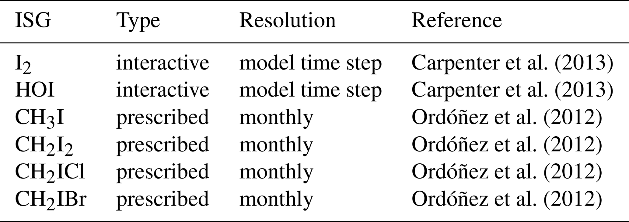
Following Ordóñez et al. (2012), the organic iodocarbons have been obtained from the inventory of Bell et al. (2002) for CH₃I and from the 1-D model estimates of Jones et al. (2010) for CH₂I₂, CH₂ICl, and CH₂IBr. Organic ISGs have been parameterized in Ordóñez et al. (2012) by a biogenic chlorophyll-a (chl-a) dependent source in the tropical oceans (McClain et al., 2004). In our scheme, organic emissions are prescribed on a monthly basis. To simulate the long-term period, we repeat organic emissions fluxes at the beginning of every model year, so any interannual variability is not included.

Iodocarbon source fluxes were directly extracted from the GEOS-Chem model (v10-01) at a resolution of a 2 × 2.5^∘, including updates to both iodine and bromine chemistry from Sherwen et al. (2016c) and Schmidt et al. (2016), and interpolated on the SOCOL-AERv2-I horizontal grid (T42). The inorganic HOI $/$ I₂ fluxes are interactively calculated in the model using the numerical parametrization of Carpenter et al. (2013) and global sea surface iodide concentration calculated following MacDonald et al. (2014). To derive HOI $/$ I₂ fluxes this parametrization utilizes the model fields of near-surface ozone (at the model level closest to the surface), surface wind speed, and SST.

The parametrization for the emission fluxes of F_HOI and $F_{I_{\mathrm{2}}}$ (in nmol m⁻² d⁻¹) as a function of the surface ozone mixing ratio ${\mathit{\chi }}_{{\mathrm{O}}_{\mathrm{3},\mathrm{surf}}}$ (in ppbv) are given by

$$\begin{array}{}\text{(1)}& {\displaystyle }\begin{array}{rl}{F}_{\mathrm{HOI}}& ={\mathit{\chi }}_{{\mathrm{O}}_{\mathrm{3},\mathrm{surf}}}\times (\mathrm{4.15}\times {\mathrm{10}}^{\mathrm{5}}\times (M_{{\mathrm{I}}_{\mathrm{aq}}^{-}}^{\mathrm{1}/\mathrm{2}}/W_{\mathrm{s}})\\ & -(\mathrm{20.6}/W_{\mathrm{s}})-\mathrm{23}\mathrm{600}\times M_{{\mathrm{I}}_{\mathrm{aq}}^{-}}^{\mathrm{1}/\mathrm{2}}),\end{array}\text{(2)}& {\displaystyle }{F}_{{\mathrm{I}}_{\mathrm{2}}}={\mathit{\chi }}_{{\mathrm{O}}_{\mathrm{3},\mathrm{surf}}}\times M_{{\mathrm{I}}_{\mathrm{aq}}^{-}}^{\mathrm{1.3}}\times (\mathrm{1.74}\times {\mathrm{10}}^{\mathrm{9}}-\mathrm{6.54}\times {\mathrm{10}}^{\mathrm{8}}\times {\mathrm{lnW}}_{\mathrm{s}}),\end{array}$$

where W_s is the surface wind speed (in m s⁻¹) and $M_{{\mathrm{I}}_{\mathrm{aq}}^{-}}$ is the sea surface iodide concentration expressed as molarity (mol dm⁻³)

$$\begin{array}{}\text{(3)}& M_{I_{\mathrm{aq}}^{-}}=\mathrm{1.46}\times {\mathrm{10}}^{\mathrm{6}}\exp (-\mathrm{9134}/T_{\mathrm{ss}})\end{array}$$

with sea surface temperature T_ss in K.

It is important to note that this parameterization is intended for calculating I₂ and HOI fluxes at wind speeds below 14 m s⁻¹ (higher wind speeds lead to negative values of fluxes) since it is based on the approximation of measurements and there are no measurements when a storm occurs. Also, it should be mentioned that turbulent mixing of the interfacial layer with bulk seawater reduces the proportion of I₂ and HOI escaping into the atmosphere; therefore fluxes decrease with the wind speed (MacDonald et al., 2014). The obtained inorganic ISGs fluxes in the SOCOL-AERv2-I exceed GEOS-Chem and CAM-Chem emissions because SOCOL-AERv2-I overestimates near-surface O₃ (Revell et al., 2018). When we compared the ground-level ozone fields from SOCOL and GEOS-chem, we found that for most regions where HOI $/$ I₂ emissions are produced, the overestimation of ground-level ozone in SOCOL is ∼100 %. To ameliorate this bias, the surface ozone used within the parameterization was scaled by 0.5. This halved the emission, making HOI $/$ I₂ fluxes comparable: ∼2.4 Tg (I)/year in SOCOL-AERv2-I and ∼2.2 Tg (I)/year in GEOS-chem (Sherwen et al., 2016c). Since there is an uncertainty in inorganic iodine emissions (Chance et al., 2014; Sherwen et al., 2016c), such a difference in emissions between models is admissible. Iodocarbon source fluxes in both SOCOL-AERv2-I and GEOS-chem are identical and correspond to 0.5 Tg (I)/year. Iodine emission fluxes used in CCM SOCOL-AERv2-I are demonstrated in Fig. 1.

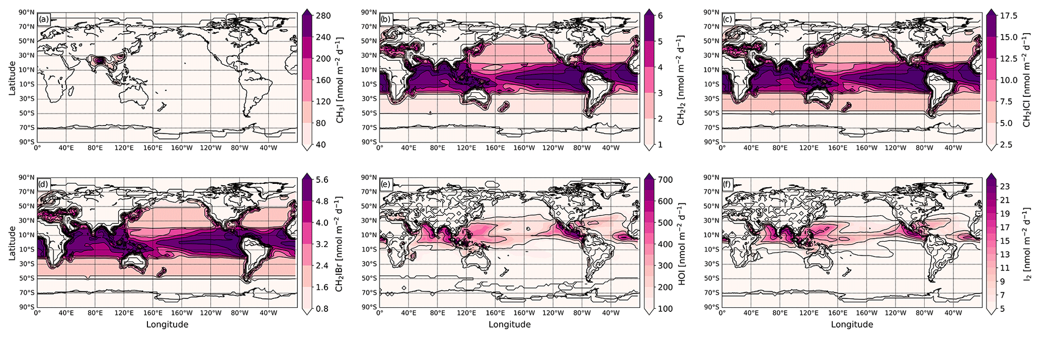
Figure 1 Annual-mean emission fluxes of organic (CH₃I, a; CH₂I₂, b; CH₂ICl, c; and CH₂IBr, d) and inorganic (HOI e and I₂ f) iodine source gases (in nmol m⁻² d⁻¹) used in SOCOL-AERv2-I.

As it is seen in Fig. 1, the sum inorganic fluxes of ISGs [HOI + I₂] is roughly 3 times higher than that of organic fluxes [CH₃I + CH₂I₂ + CH₂ICl + CH₂IBr] of ISGs that is corresponding well with Carpenter et al. (2013).

Chemical compounds involved in the iodine chemistry scheme in SOCOL-AERv2-I are presented in Table 2.

Burkholder et al. (2015)Burkholder et al. (2015)Ordóñez et al. (2012)Burkholder et al. (2015)Badia et al. (2019)Badia et al. (2019)Wagman et al. (1989)Wagman et al. (1989)Badia et al. (2019)Badia et al. (2019)Badia et al. (2019)Burkholder et al. (2015)Burkholder et al. (2015)Hilal et al. (2008)Hilal et al. (2008)

Table 2 The iodine species considered in SOCOL-AERv2-I.

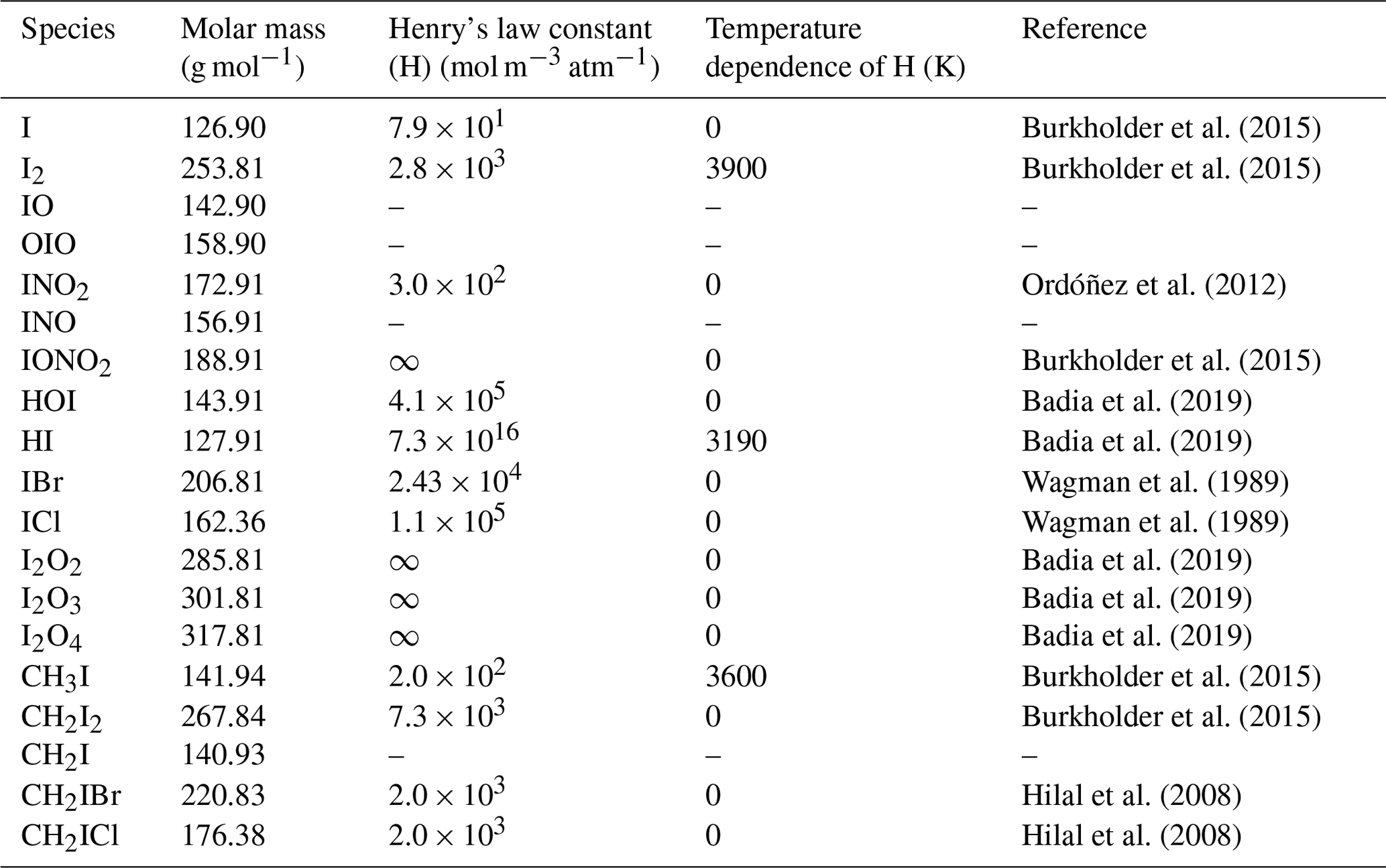
A dash means that Henry's law constant is unavailable. For IONO₂ and I_xO_y Henry's law constants are assumed to be infinity and represented by a very large number.

Overall, 19 iodine species are included in the current version of the iodine chemistry scheme of SOCOL-AERv2-I: 6 iodine source gases (ISGs) and 13 product gases (PGs) including two species (HOI and I₂), which are both being emitted and chemically produced. Photolysis rates and reaction cross sections for iodine species were taken from Burkholder et al. (2015). An exception is made only for the photolysis rates of higher iodine oxide species, such as I₂O₂, I₂O₃, and I₂O₄, where we followed the recommendations of Davis et al. (1996) and Vogt et al. (1999), who suggested using photolysis rates of iodine oxides 9 times higher than those of Cl₂O₂. This is a more simplified approach than used in CAM-chem, where cross sections for I₂O₂ and I₂O₃ are adopted from Gómez-Martín et al. (2005), and for I₂O₄ the used spectrum is measured at the University of Leeds (Saiz-Lopez et al., 2014). In GEOS-chem, the cross sections for higher iodine oxides are equal to those of IONO₂ (Sherwen et al., 2016a) based on the assumption made by Bloss et al. (2010). In our scheme, we checked this possibility too and found that there is no noticeable difference between using IONO₂ photolysis rates or 9*Cl₂O₂ photolysis rates as substitutes for unknown photolysis rates of higher iodine oxides. The Henry's law constant of IONO₂ is taken in SOCOL-AERv2-I to be infinity by analogous to BrONO₂ and ClONO₂ (1 × 10³⁰ mol m⁻³ atm⁻¹). The Henry's law constant of I_xO_y is infinity and represented by 2.65 × 10¹⁸ mol m⁻³ atm⁻¹ (Badia et al., 2019). The Henry's law constant of INO₂ is equal to that of BrNO₂ presented in Ordóñez et al. (2012).

The full iodine reaction scheme, composed of 61 gas-phase chemical reactions including 17 photolysis reactions and 4 heterogeneous reactions proceeding on tropospheric cloud ice, is presented in Table 3.

Ordóñez et al. (2012)Ordóñez et al. (2012)Burkholder et al. (2015)Ordóñez et al. (2012)Burkholder et al. (2015)Burkholder et al. (2015)Saiz-Lopez et al. (2014)Badia et al. (2019)Burkholder et al. (2015)Saiz-Lopez et al. (2014)Badia et al. (2019)Badia et al. (2019)Saiz-Lopez et al. (2014)Burkholder et al. (2015)Burkholder et al. (2015)Badia et al. (2019)Badia et al. (2019)Saiz-Lopez et al. (2014)Saiz-Lopez et al. (2014)Burkholder et al. (2015)Burkholder et al. (2015)Burkholder et al. (2015)Burkholder et al. (2015)Saiz-Lopez et al. (2015)Gravestock et al. (2010)Saiz-Lopez et al. (2014)Saiz-Lopez et al. (2014)Badia et al. (2019)Badia et al. (2019)Saiz-Lopez et al. (2014)Saiz-Lopez et al. (2014)Saiz-Lopez et al. (2014)Saiz-Lopez et al. (2014)Saiz-Lopez et al. (2014)Saiz-Lopez et al. (2014)Saiz-Lopez et al. (2014)Ordóñez et al. (2012)Ordóñez et al. (2012)Badia et al. (2019)Burkholder et al. (2015)Badia et al. (2019)Burkholder et al. (2015)Burkholder et al. (2015)Burkholder et al. (2015)Burkholder et al. (2015)Burkholder et al. (2015)Burkholder et al. (2015)Burkholder et al. (2015)Burkholder et al. (2015)Burkholder et al. (2015)Burkholder et al. (2015)Burkholder et al. (2015)Burkholder et al. (2015)Burkholder et al. (2015)Davis et al. (1996)Davis et al. (1996)Davis et al. (1996)Burkholder et al. (2015)Burkholder et al. (2015)Burkholder et al. (2015)Burkholder et al. (2015)Saiz-Lopez et al. (2015)Saiz-Lopez et al. (2015)Saiz-Lopez et al. (2015)Saiz-Lopez et al. (2015)

Table 3 The list of chemical reactions with iodine included to SOCOL-AERv2-I.

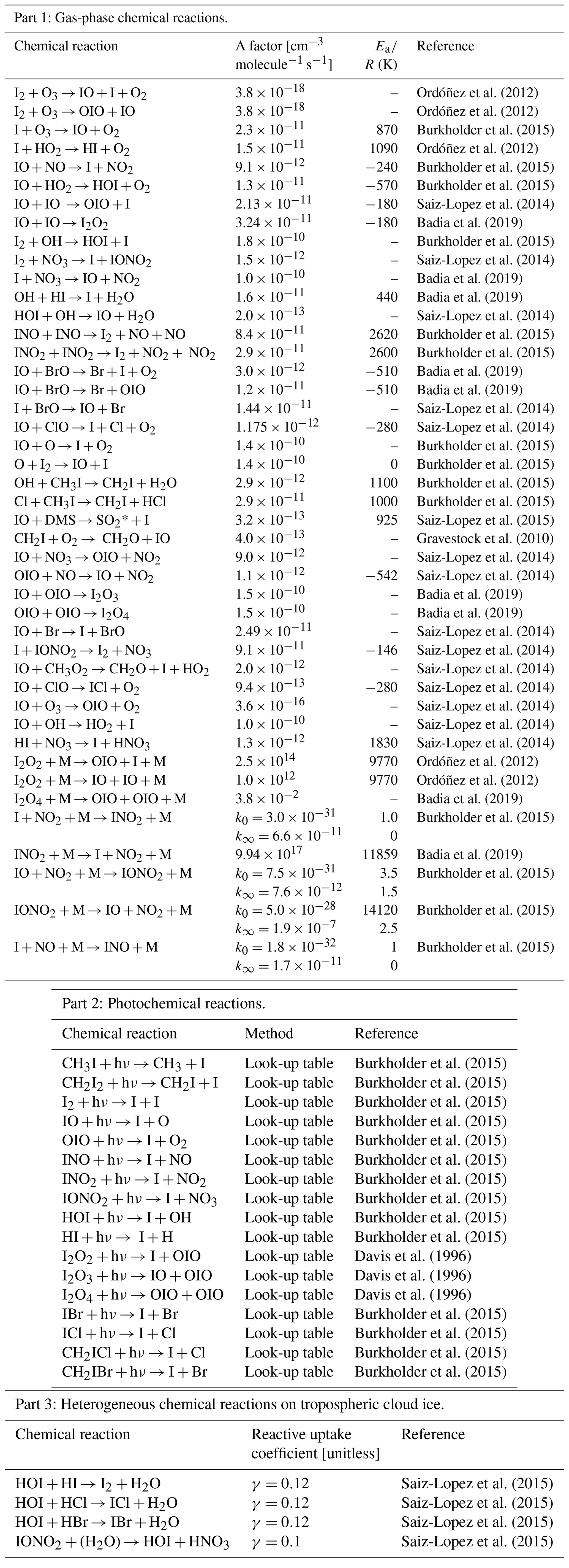
A factor: the pre-exponential factor. E_a: the activation energy. R: the universal gas constant. SO₂ instead of DMSO is used (DMSO is absent in SOCOL-AERv2-I). k₀: low-pressure limit (cm⁶ molecule⁻² s⁻¹). k_∞: high-pressure limit (cm³ molecule⁻¹ s⁻¹).

We briefly review SOCOL's chlorine and bromine reactions because of their interaction with iodine chemistry. Apart from reactions involving iodine, there are about 100 gas-phase and 11 heterogeneous reactions on sulfates and polar stratospheric clouds (PSCs) for chlorine species and about 50 gas-phase and 4 heterogeneous reactions on sulfates and polar stratospheric clouds (PSCs) for bromine species. The total gas-phase chlorine (Cl_tot) and bromine (Br_tot) in the current version of the model are

$$\begin{array}{rl}& {\mathrm{Cl}}_{\mathrm{tot}}=\mathrm{ClO}+\mathrm{Cl}+\mathrm{2}\times {\mathrm{Cl}}_{\mathrm{2}}+{\mathrm{ClNO}}_{\mathrm{3}}+\mathrm{HOCl}+\mathrm{HCl}+\mathrm{2}\\ & \times {\mathrm{Cl}}_{\mathrm{2}}{\mathrm{O}}_{\mathrm{2}}+\mathrm{BrCl}+\mathrm{3}\times \mathrm{CFC}-\mathrm{11}+\mathrm{2}\times \mathrm{CFC}-\mathrm{12}+\mathrm{3}\\ & \times \mathrm{CFC}-\mathrm{113}+\mathrm{2}\times \mathrm{CFC}-\mathrm{114}+\mathrm{CFC}-\mathrm{115}+\mathrm{4}\times {\mathrm{CCl}}_{\mathrm{4}}\\ & +\mathrm{3}\times {\mathrm{CH}}_{\mathrm{3}}{\mathrm{CCl}}_{\mathrm{3}}+\mathrm{HCFC}-\mathrm{22}+\mathrm{2}\times \mathrm{HCFC}-\mathrm{141}\mathrm{B}\\ & +\mathrm{HCFC}-\mathrm{142}\mathrm{B}+\mathrm{H}-\mathrm{1211}+{\mathrm{CH}}_{\mathrm{3}}\mathrm{Cl}+\mathrm{2}\times \mathrm{HCFC}-\mathrm{21}\\ & +\mathrm{2}\times \mathrm{HCFC}-\mathrm{123}+\mathrm{HCFC}-\mathrm{31}+\mathrm{ICl}+{\mathrm{CH}}_{\mathrm{2}}\mathrm{ICl}\\ & \mathrm{and}\\ & {\mathrm{Br}}_{\mathrm{tot}}=\mathrm{Br}+\mathrm{BrO}+\mathrm{2}\times {\mathrm{Br}}_{\mathrm{2}}+\mathrm{BrCl}+{\mathrm{BrNO}}_{\mathrm{3}}+\mathrm{HBr}+\mathrm{2}\\ & \times {\mathrm{CH}}_{\mathrm{2}}{\mathrm{Br}}_{\mathrm{2}}+{\mathrm{CH}}_{\mathrm{3}}\mathrm{Br}+{\mathrm{CBrF}}_{\mathrm{3}}+\mathrm{3}\times {\mathrm{CHBr}}_{\mathrm{3}}+\mathrm{HOBr}+\mathrm{H}\\ & -\mathrm{1301}+\mathrm{H}-\mathrm{1211}+\mathrm{2}\times \mathrm{H}-\mathrm{2402}+\mathrm{IBr}+{\mathrm{CH}}_{\mathrm{2}}\mathrm{IBr}.\end{array}$$

Similar to the iodine schemes in CAM-chem (Ordóñez et al., 2012) and GEOS-Chem (Sherwen et al., 2016a), we implemented the free molecular transfer approximation of McFiggans et al. (2000). This allows the introduction of the iodine scavenging and deposition on sea-salt and sulfate aerosols as well as effective ice uptake (removal)/reactive ice uptake (recycling) on a surface of tropospheric cloud ice crystals (Fernandez et al., 2014; Saiz-Lopez et al., 2014, 2015). The transfer coefficient (s⁻¹) is calculated as follows:

$$\begin{array}{}\text{(4)}& {\displaystyle }k={\displaystyle \frac{\mathrm{1}}{\mathrm{4}}}\mathit{\gamma }\langle c\rangle A,\end{array}$$

where γ is the effective/reactive uptake coefficient (see Table 3), A is the surface area density (in cm² cm⁻³) of the particles on which the deposition occurs, $\langle c\rangle =(\mathrm{8}RT/\mathit{\pi }M{)}^{\mathrm{1}/\mathrm{2}}$ is the mean thermal molecular speed (in cm s⁻¹) of molecules with molar mass M (in kg mol⁻¹) at absolute temperature T (in K), and R=8.3145 J mol⁻¹ K⁻¹.

In SOCOL-AERv2-I, sea-salt aerosols are prescribed by monthly means from observational data and aqueous sulfuric acid aerosols are calculated interactively; from both, surface area densities (SADs) are available. However, there is no readily available SAD for cloud ice in SOCOL-AERv2-I. Therefore, we calculate the effective radius R_eff (in µm) of ice crystals following Heymsfield et al. (2014):

$$\begin{array}{}\text{(5)}& {\displaystyle }{R}_{\mathrm{eff}}=\mathit{\alpha }\exp \left(\mathit{\beta }{T}_c\right),\end{array}$$

where T_c is the temperature (in ^∘C); α=154.2 and β=0.0152 for −56 ^∘C $<T<$ 0 ^∘C; α=4.5872 × 10⁴ and β=0.117 for −71 ^∘C $<T<$ −56 ^∘C; and α=41.65 and β=0.0184 for −85 ^∘C $<T<$ −71^∘C. Following Holmes et al. (2019), the SAD for ice particles (in cm² cm⁻³) is calculated from (R_eff) as follows:

$$\begin{array}{}\text{(6)}& {\displaystyle }{\mathrm{SAD}}_{\mathrm{ice}}=\mathrm{6.75}\times \mathrm{IWC}/\left(\mathit{\rho }{R}_{\mathrm{eff}}\right),\end{array}$$

where ρ is the density of ice (9.167 × 10⁻⁴ kg cm⁻³) and IWC is the ice water content, i.e., the mass of ice per volume of air in the cloud (in kg cm⁻³).

Since the timescale of the physical process of removal/recycling of iodine is shorter than the model time step (2 h), using an explicit integration scheme may result in excessive removal/recycling of iodine species leading to errors (such as negative concentrations). To avoid this, we decided to implement a simple implicit scheme:

$$\begin{array}{}\text{(7)}& {\displaystyle }{C}_{\mathrm{1}}=C_{\mathrm{0}}/(\mathrm{1}+K\times \mathrm{\Delta }t),\end{array}$$

where C₀ is the initial concentration, K is the transfer coefficient, C₁ is the final concentration, and Δt is the model time step for chemistry. This scheme avoids producing negative C₁.

As effective uptake coefficients (γ), we applied ${\mathit{\gamma }}_{{\mathrm{IONO}}_{\mathrm{2}}}=\mathrm{0.01}$, ${\mathit{\gamma }}_{{\mathrm{INO}}_{\mathrm{2}}}=\mathrm{0.02}$, γ_HOI=0.06, ${\mathit{\gamma }}_{{\mathrm{I}}_{\mathrm{2}}{\mathrm{O}}_{\mathrm{2}}}={\mathit{\gamma }}_{{\mathrm{I}}_{\mathrm{2}}{\mathrm{O}}_{\mathrm{3}}}={\mathit{\gamma }}_{{\mathrm{I}}_{\mathrm{2}}{\mathrm{O}}_{\mathrm{4}}}=\mathrm{0.01}$ to model an effective uptake and removal of iodine species on sea-salt aerosols (Ordóñez et al., 2012).

Since γ values for sulfate aerosols are currently unknown and if we consider effective uptake on sulfate aerosols with the same gamma as for sea-salt aerosols, we would obtain modeled I_y values with a large bias (X %) against observations for sulfate particles. γ values for sea-salt aerosols in SOCOL-AERv2-I were divided by 100 (as the amount of iodine to be removed on tropospheric sulfate aerosols is assumed to be 100 less than for sea salt), which brought the iodine from SOCOL-AERv2-I to be closer to available observations. For effective ice uptake of iodine, γ values are taken to be the same as in CAM-chem (Saiz-Lopez et al., 2014): γ_HOI=0.0003; ${\mathit{\gamma }}_{{\mathrm{IONO}}_{\mathrm{2}}}=\mathrm{0.005}$; γ_HI=0.02. The removal on all presented surfaces is operated only within the troposphere (it is confined by the tropopause height). It must be mentioned that the values of effective uptake coefficients for iodine species for different types of surfaces are highly uncertain (Saiz-Lopez et al., 2014). It is worth saying that we only consider the deposition on sea-salt and sulfate aerosols and did not implement any heterogeneous recycling of iodine species on sea-salt aerosols like those described in Vogt et al. (1996, 1999), Ordóñez et al. (2012), Saiz-Lopez et al. (2014), and Tham et al. (2021). It should be noted that the lack of recycling on sea-salt aerosols may affect the I_y burden and the amount of stratospheric iodine injection. Yet, it requires additional study to estimate it quantitatively.
In the heterogeneous recycling mechanism on ice, reactive uptake coefficients for cloud ice are taken as follows: γ_HOI=0.12; ${\mathit{\gamma }}_{{\mathrm{IONO}}_{\mathrm{2}}}=\mathrm{0.1}$ (see Saiz-Lopez et al., 2015 supplements). Transfer coefficients for heterogeneous reactions (see Table 3) are also calculated by free molecular transfer approximation (McFiggans et al., 2000) but using reactive uptake coefficients. The reactive ice uptake and recycling of HOI and IONO₂ is applied in SOCOL-AERv2-I after effective ice uptake and removal of HOI, IONO₂, and HI. The sequence of removal/recycling processes is unclear but the chosen sequence shows reasonable results. Also, it should be noted here that there is no evidence of reactive uptake and recycling of iodine species in liquid clouds, and in our scheme, we use it only for ice crystals as was done by Saiz-Lopez et al. (2015).

2.3 Conducted experiments

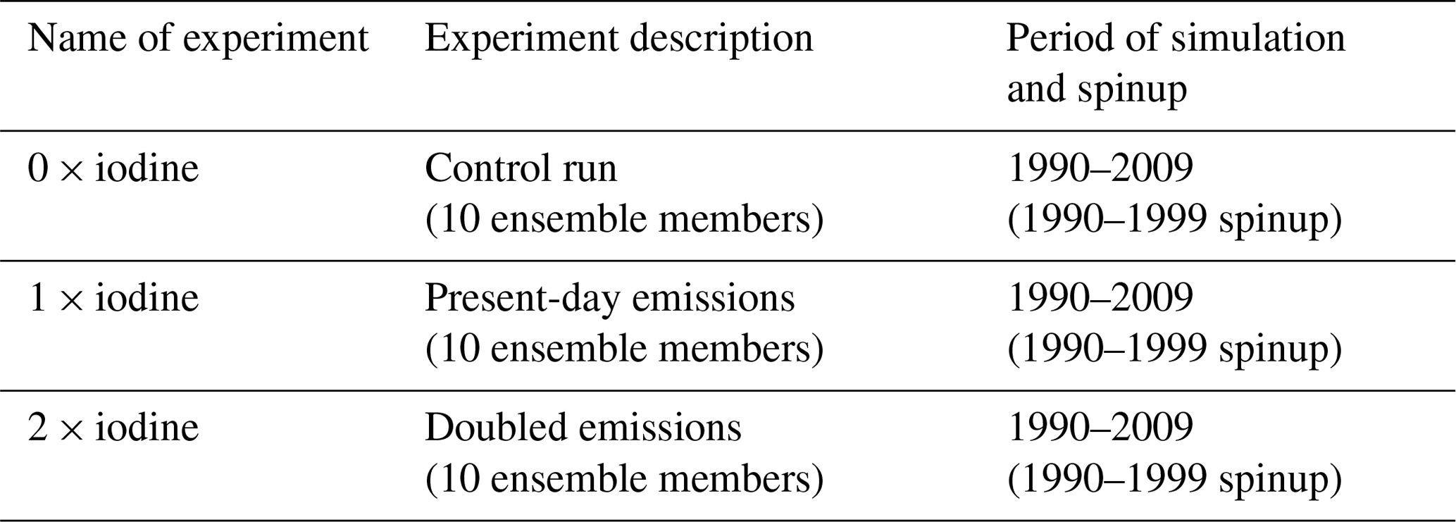
To evaluate the iodine chemistry scheme of SOCOL-AERv2-I as well as to estimate the influence of iodine chemistry on ozone we designed and carried out three transient numerical experiments. The first one is the control experiment where iodine emissions are set to zero. For the second experiment (1 × iodine), we applied a basic configuration with the present-day iodine emissions. These experiments are used to evaluate the veracity of iodine in SOCOL-AERv2-I and to estimate the influence of iodine chemistry on present-day ozone climatology.

To assess whether the potential intensification of iodine emissions in the future will have a tangible effect on the ozone layer, we designed a sensitivity experiment (to verify the sensitivity of ozone to iodine) in which all iodine emissions are doubled to present-day emissions (2 × iodine). In essence, it could be assumed as a worst-case scenario compared to the present-day emissions that might become closer to reality by the middle of this century if the rise of emissions presented by Cuevas et al. (2018) and Legrand et al. (2018) continued despite no dramatic forecast of iodine emission’s evolution being made by Iglesias-Suarez et al. (2020). The iodine content in the future is also difficult to predict due to a huge discrepancy between scenarios for the future evolution of iodine precursors like tropospheric ozone (Archibald et al., 2020) and SST (Taylor et al., 2012). Albeit, it should be said that in our study this assumption was used only to verify the sensitivity of ozone to iodine chemistry. The sensitivity of ozone to the increase in the iodine emissions was characterized by comparing experiments with 2 ×  and 1 × loading of iodine. All experiments were run for the 1990–2009 period including the 10-year spinup (1990–1999) from the initial conditions that is necessary for iodine to reach the quasi-equilibrium state. The spinup period was excluded from further analysis. Each experiment consists of 10 ensemble members with a 1-month perturbation of initial CO₂ concentration to get 10 different atmospheric realizations and to calculate the statistical significance of the iodine influence on ozone using Student's t test. The summary of the experimental setup can be found in Table 4.

Table 4 The experiments with SOCOL-AERv2-I.

3 Results of simulation

3.1 Evaluation of the iodine from SOCOL-AERv2-I against CAM-chem and observations

The total gas-phase inorganic I_y in both 2 × iodine and 1 × iodine experiments of SOCOL-AERv2-I averaged over the tropics (20^∘ N–20^∘ S), for the 2000–2009 period and 10 ensemble members, is presented in Fig. 2.

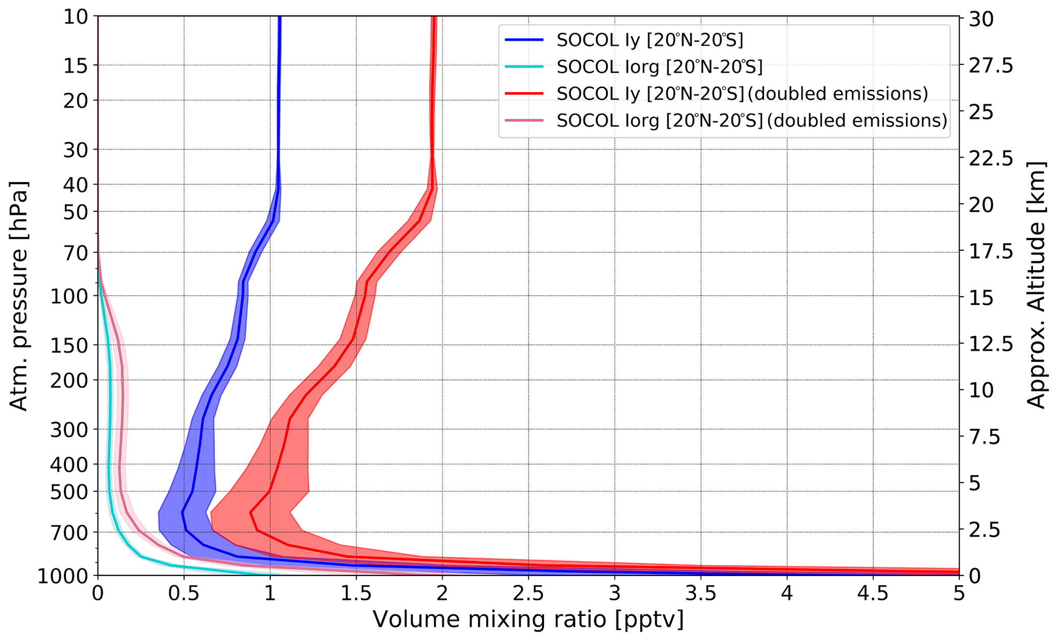
Figure 2 Modeled vertical distribution of total organic (I_org) and inorganic (I_y) gas-phase iodine simulated with SOCOL-AERv2-I averaged over the tropics (20^∘ N–20^∘ S), for the 2000–2009 period and 10 ensemble members. Red curve: I_y from the experiment 2 × iodine. Blue curve: I_y from the experiment 1 × iodine. Light red and blue curves: I_org from 2 × iodine and 1 × iodine experiments, correspondingly. Shadings represent a standard deviation of tropical iodine (20^∘ N–20^∘ S).

The I_y was calculated as a sum of inorganic iodine compounds presented in the SOCOL-AERv2-I’s iodine scheme: I_y = IO + I + OIO + HOI + 2 ×  I₂ + HI + INO + INO₂ + 2 ×  (I₂O₂ + I₂O₃ + I₂O₄) + ICl+ IBr + IONO₂ + CH₂I. I_org is calculated as a sum of all organic compounds in SOCOL-AERv2-I: I_org = CH₃I + 2 ×  CH₂I₂ + CH₂ICl + CH₂IBr. The standard deviation of iodine between ensemble members is found to be less than 1 %. In the lower troposphere, the I_y is rapidly dropping with altitude until about 600 hPa following the washout that is most effective at this layer. In the upper troposphere (above 200 hPa), I_y increases after the initiation of the recycling heterogeneous mechanism on ice that works at these altitudes in the tropics because the availability of cloud ice is essential. The recycling on cloud ice mostly defines the amount of inorganic iodine injected into the stratosphere because it competes with the washout of reservoir species by converting reservoirs into species with lower washout rates and thus increasing the residence lifetime. The stratospheric I_y shows an increase until about 50 hPa and then stays constant because there is no deposition of iodine above this layer. The simulated stratospheric I_y by SOCOL-AER2-I agrees well with the results of the CAM-chem model in the lowermost stratosphere showing about 0.75–0.8 pptv of I_y; however, it becomes higher in the middle stratosphere than in Saiz-Lopez et al. (2015). We suggest that it might have resulted from model non-conservative transport scheme and dynamics, for example, the deep tropical convection cells over the area of iodine production that overcomes the deposition velocity enhancing the stratospheric iodine loading. Higher values of I_y in the stratosphere relative to the upper and middle troposphere can be also explained by the rapid tropospheric sinks and relatively slow transport of I_y into the troposphere. A hard upper border in SOCOL-AER2-I that prevents chemical species from going through it also might impact the profile. Nevertheless, the stratospheric I_y abundance calculated with SOCOL-AER2-I does not exceed 1.05 pptv and corresponds well to the estimation given by Solomon et al. (1994), although it is slightly larger than the most recent assessment from WMO (2018) (0.8 pptv I_y).

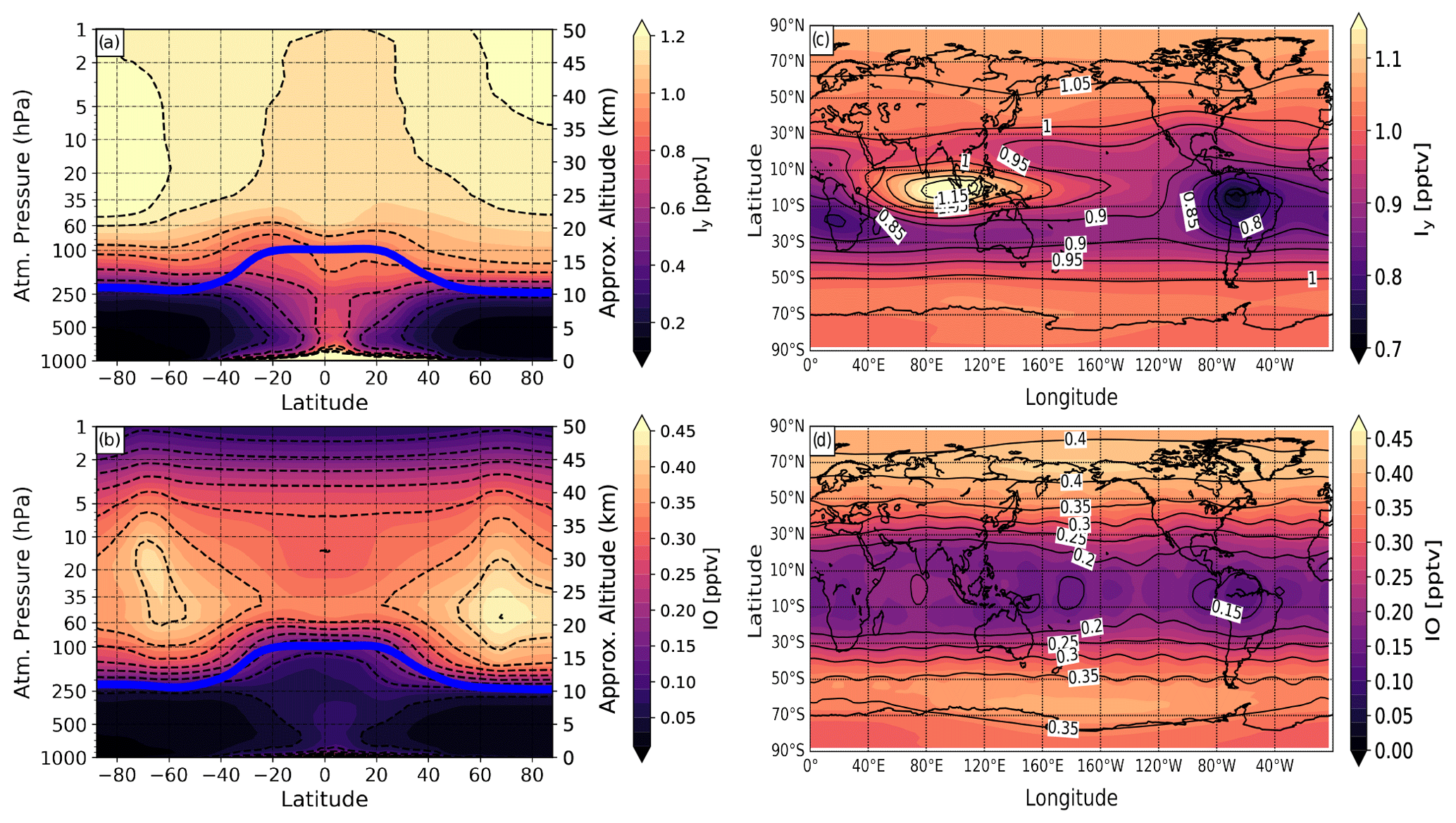
Figure 3 Modeled vertical distribution and global map of total inorganic gas-phase iodine (I_y) and iodine monoxide (IO) simulated with SOCOL-AERv2-I from the experiment with present-day iodine emissions (1× iodine), averaged for the 2000–2009 period and 10 ensemble members. (a, b) Zonal-mean vertical distributions of I_y and IO. (c, d) Global maps of I_y and IO averaged for 100–70 hPa region. Blue solid line in (a) and (b): annual mean tropopause height.

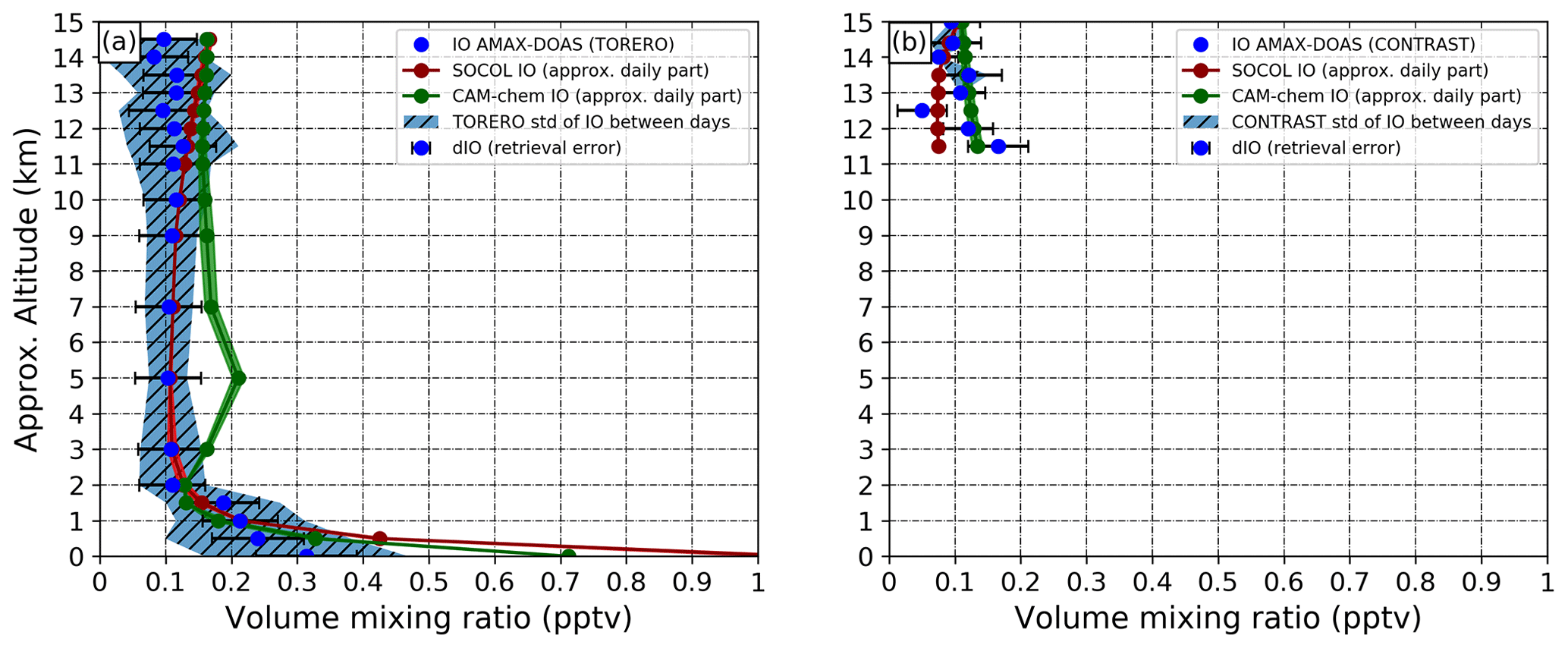
Figure 4 January–February averages of modeled and observed IO in the tropical troposphere [15^∘ N–15^∘ S] for (a) the TORERO campaign from Costa Rica (January–February 2012, 10^∘ N–40^∘ S, 250–285^∘ E), and (b) the CONTRAST campaign from Guam (January–February 2014, 40^∘ N–15^∘ S, 115–175^∘ E). Red line: IO from SOCOL-AERv2-I. Green line: IO from CAM-chem. Blue dots: IO observed by AMAX-DOAS. Shadings: IO standard deviations of all modeled and measured IO during the January–February period.

Figure 3 presents the vertical distributions of I_y and IO at all latitudes and global maps of I_y and IO averaged for the lower stratosphere (100–70 hPa). I_y and IO have the highest mixing ratio at the polar regions of the stratosphere due to transport carried out by the Brewer–Dobson circulation (BDC). The larger stratospheric values of IO at high latitudes are also related to the higher O₃ abundance at those locations. At the tropics, there are two pronounced areas with a higher (over the Indian ocean) and with a lower (over South America) I_y mixing ratio as depicted in Fig. 3c. Their formation might have resulted from different convection patterns (weaker/stronger) over these areas. Also, the area with a higher stratospheric I_y burden is located right over the region with higher surface emissions of HOI $/$ I₂ (see Fig. 1). In the troposphere, the iodine level is decreasing toward the poles and far from the iodine source regions. The iodine distribution demonstrates the highest mixing ratio of iodine in the lower stratosphere over middle-to-high latitudes with a maximum I_y of more than 1.15 pptv in the polar region of the Northern Hemisphere and about 1 pptv in the Southern Hemisphere. The IO has two maximums of about 0.4 pptv in the lower-to-middle stratosphere and high latitudes. Also, note that IO decreases at higher levels of the stratosphere exhibiting more than 5 times less abundance than in the lower stratosphere, which might result from decreasing the efficiency of O₃–I reactions. We compared the mixing ratio of iodine compounds with some of the local measurements mentioned above. The modeled reactive IO over Scandinavia (70^∘ N; 20^∘ E) in March is >0.45 pptv at 17 km (monthly-mean value), which is in agreement with IO simulated with a box model that was partly initialized with the IO retrieved by balloon flights (a daytime concentration of ∼0.65 pptv at 17 km) (Pundt et al., 1998). Yet, the balloon-borne measured upper limit of IO mixing ratio is 0.2 pptv (Pundt et al., 1998), which is more than 2 times lower than the IO mixing ratio simulated with SOCOL-AER2-I. SOCOL-AER2-I also captures well the I_y estimated by the box model (Pundt et al., 1998) showing a mixing ratio of 1–1.1 pptv. Also, IO simulated with SOCOL-AERv2-I corresponds well with DOAS measurements over Spitsbergen island (79^∘ N; 12^∘ E) in March (Wittrock et al., 2000), showing >0.48 pptv in the lower stratosphere. Further, we compare the iodine monoxide (IO) obtained by SOCOL-AER2-I with the one from the CAM-chem model and the recent aircraft observations with AMAX-DOAS conducted during the TORERO and CONTRAST campaign (Volkamer et al., 2015; Pan et al., 2017). The results are shown in Fig. 4.

We compare the observed and measured IO only over the tropics (15^∘ N–15^∘ S) as extratropical measurements from both campaigns are scarcer and the comparison will be biased. Modeled IO in Fig. 4 has been obtained by doubling monthly averaged IO, which is fair to do for tropics as during nighttime the IO concentration is negligible. Also, the observations are given as so-called footprints to get profiles for each day; they were averaged for certain altitudes designated in Fig. 4 as blue points. The averaged values for Fig. 4 are obtained by averaging all measurements taken in the nearby altitude ranges. The IO from both models is sampled at the same altitudes as measurements to conduct an equitable comparison. It should be noted that from the CONTRAST campaign, tropical IO measurements in the upper troposphere are only available. Both SOCOL-AERv2-I and CAM-chem overestimate observations from the TORERO campaign at near-surface levels. The sharp decrease in observed and modeled IO from both models is similar until 2 km, showing compatible IO mixing ratios. At 5 km, CAM-chem shows a maximum IO mixing ratio of about 0.2 pptv that is not seen in SOCOL-AERv2-I and observations. CAM-chem generally overestimates SOCOL-AERv2-I and observations during the TORERO campaign up to about 11–12 km. After 11 km, both models overestimate the mean of observed IO from the TORERO campaign but in general stays within the uncertainty of observations. The increase in modeled IO after 12 km might follow the recycling activity on ice, but it is not seen over the region of the CONTRAST campaign. IO from both models is generally compatible with IO measurements during the CONTRAST campaign showing the IO mixing ratio of about 0.1–0.15 pptv.

Besides, we made a comparison of modeled I_y from SOCOL-AERv2-I and CAM-chem models with the I_y derived from IO $/$ I_y ratio modeled with the University of Colorado (CU) chemical box model constrained by measured temperature, pressure, chemical concentrations, particle size distributions, and photolysis frequencies. The uncertainty in derived I_y is estimated as 30 % of the IO $/$ I_y ratio including errors in the calibration of in situ and remote sensing data and accounting for differences in the spatial scales (Wang et al., 2015; Koenig et al., 2017). IO was taken as an average of IO fields measured with AMAX-DOAS during both TORERO and CONTRAST campaigns (Volkamer et al., 2015; Pan et al., 2017; Koenig et al., 2020). Thus, the inferred I_y is based on the measured IO and modeled IO $/$ I_y. The result of this comparison is illustrated in Fig. 5.

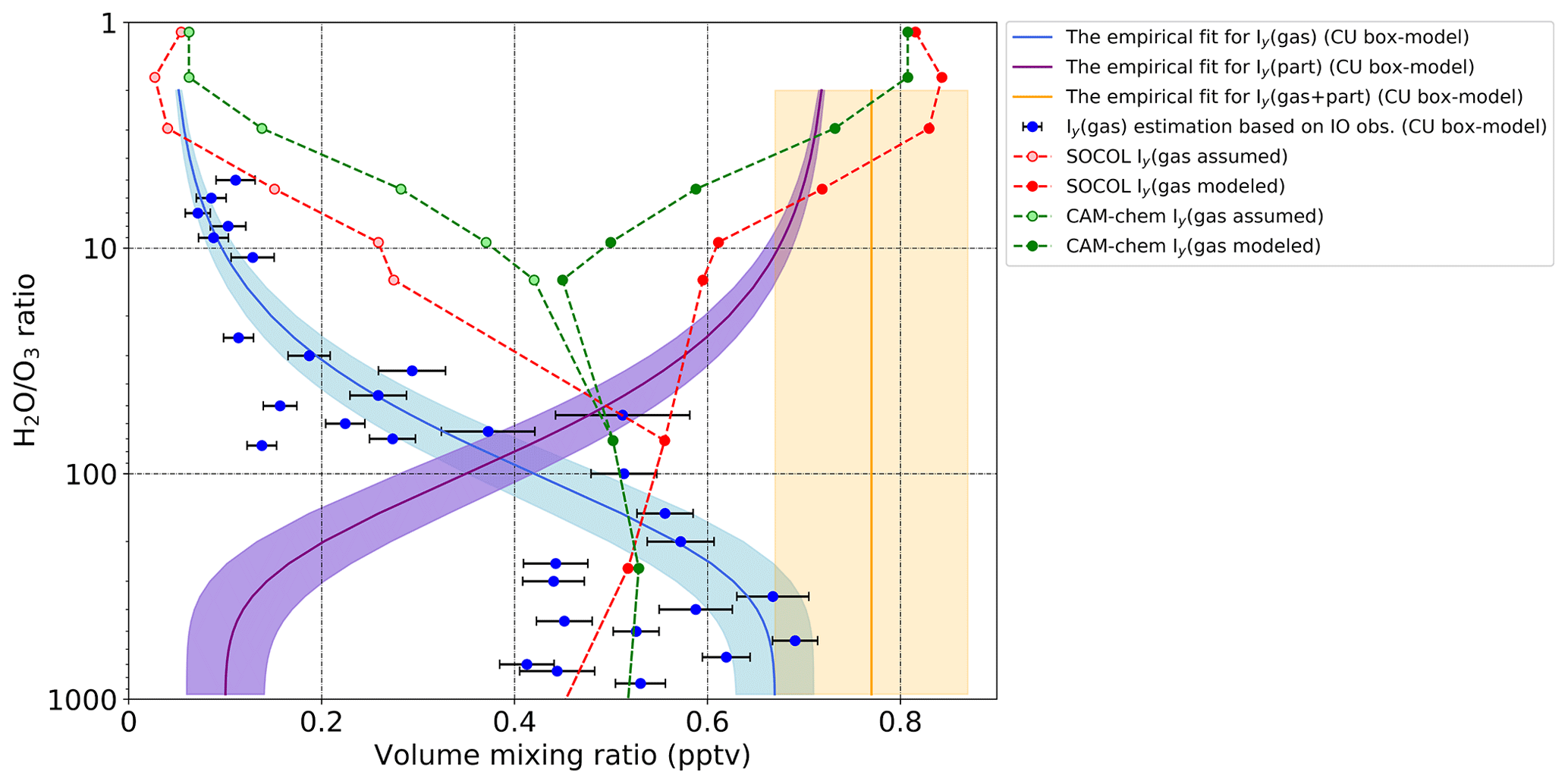
Figure 5 Total gas-phase I_y modeled with SOCOL-AERv2-I and CAM-chem as well as estimated by CU chemical box model based on AMAX-DOAS IO observations in the upper troposphere and lowermost stratosphere. All model data and observations are taken only for the region of TORERO (10^∘ N–40^∘ S, 250–285^∘ E) and CONTRAST measurements (40^∘ N–15^∘ S, 115–175^∘ E). Red and green solid and dashed lines: gas-phase I_y simulated with SOCOL-AERv2-I and CAM-chem averaged for the January–February period. Light red and light green dashed lines: assumed gas-phase I_y simulated with SOCOL-AERv2-I and CAM-chem excluding approx. iodine in the particulate phase. Blue dots: gas-phase I_y modeled by the University of Colorado (CU) chemical box model. Black error bars: the uncertainty in I_y modeled by the CU box model. Blue, purple, and orange solid lines represent the empirical fit for gas-phase I_y (gas), particulate I_y (part), and total I_y (gas + part), correspondingly. Shadings represent the uncertainty in the empirical fit.

Data were plotted with respect to the H₂O $/$ O₃ ratio as it is a good indicator to distinguish the upper troposphere air enriched in water vapor from the dehydrated air in the lower stratosphere as proposed by Koenig et al. (2020). To make CU box-model data clearer they were thinned out by averaging the data every 50 units of the H₂O $/$ O₃ ratio between 1000 and 100 of the H₂O $/$ O₃ ratio; every 5 units between 10 and 1; and every 1 unit between 10 and 1. The blue empirical fit is to a subset of the blue dots, so that the orange line is based on I_y (gas) and I_y (part) data in the upper troposphere, and the purple line is derived under the assumption of conversion. Equations to calculate empirical fit lines for experimental data can be found here (see Eqs. 2, 4, and 5 in Koenig et al., 2020, supplements).

Below the H₂O $/$ O₃ ratio of ∼70, both models capture well the I_y estimated from observations. Higher up, the red and green dashed lines represent the gas-phase I_y that is simulated with both models. Because the particulate iodine is not considered in these models, the total inorganic I_y in SOCOL-AERv2-I and CAM-chem presented here is only in the gas phase. The light red and green lines are the assumed gas-phase I_y if the estimated particulate iodine is excluded from the modeled I_y. To exclude the unknown particulate iodine, the modeled gas-phase I_y was subtracted from the 0.87 pptv of iodine that is empirical total I_y plus uncertainty of observations (0.1 pptv) (see the orange solid line and its uncertainty in Fig. 5). Such an approach can show what would be the approximate modeled gas-phase I_y if the iodine in the particulate phase was presented in models. It is seen that after the level of H₂O $/$ O₃ ratio of ∼70, the gas-phase I_y estimated from measurements rapidly decreases and reaches the value of about 0.1 pptv at the approximate altitude of the lowermost stratosphere (H₂O $/$ O₃ ratio <10). After excluding the estimated particulate iodine, the assumed modeled gas-phase I_y becomes very close to the one from the CU box model.

It bears mentioning that there is evidence that a certain part of gas-phase iodine undergoes partitioning to aerosol in the stratosphere. This mechanism is not fully understood due to a lack of measurements. Note that the approach used here is different from the simplified parameterization of IPART in CAM-Chem (Koenig et al., 2020). The assumption that the overestimation of modeled gas-phase I_y against observations is because of an absence of iodine in the particulate phase is reasonable as is seen in Fig. 5. In this work, we do not consider particulate iodine for the analysis of ozone loss as it is out of the scope of the paper. Here, we assume that the total stratospheric I_y is only in the gas phase. Nevertheless, the total amount of iodine obtained with SOCOL-AERv2-I is in good agreement with other estimates and observations and can be used in further analysis of its effect on ozone.

3.2 Iodine chemistry effect on present-day ozone climatology

We estimate the iodine effect on present-day ozone climatology by comparing the experiment with a single loading of iodine (1 × iodine), and the control experiment neglecting iodine chemistry (0 × iodine). The contribution of iodine chemistry to present-day ozone climatology estimated by the SOCOL-AERv2-I is presented in Fig. 6.

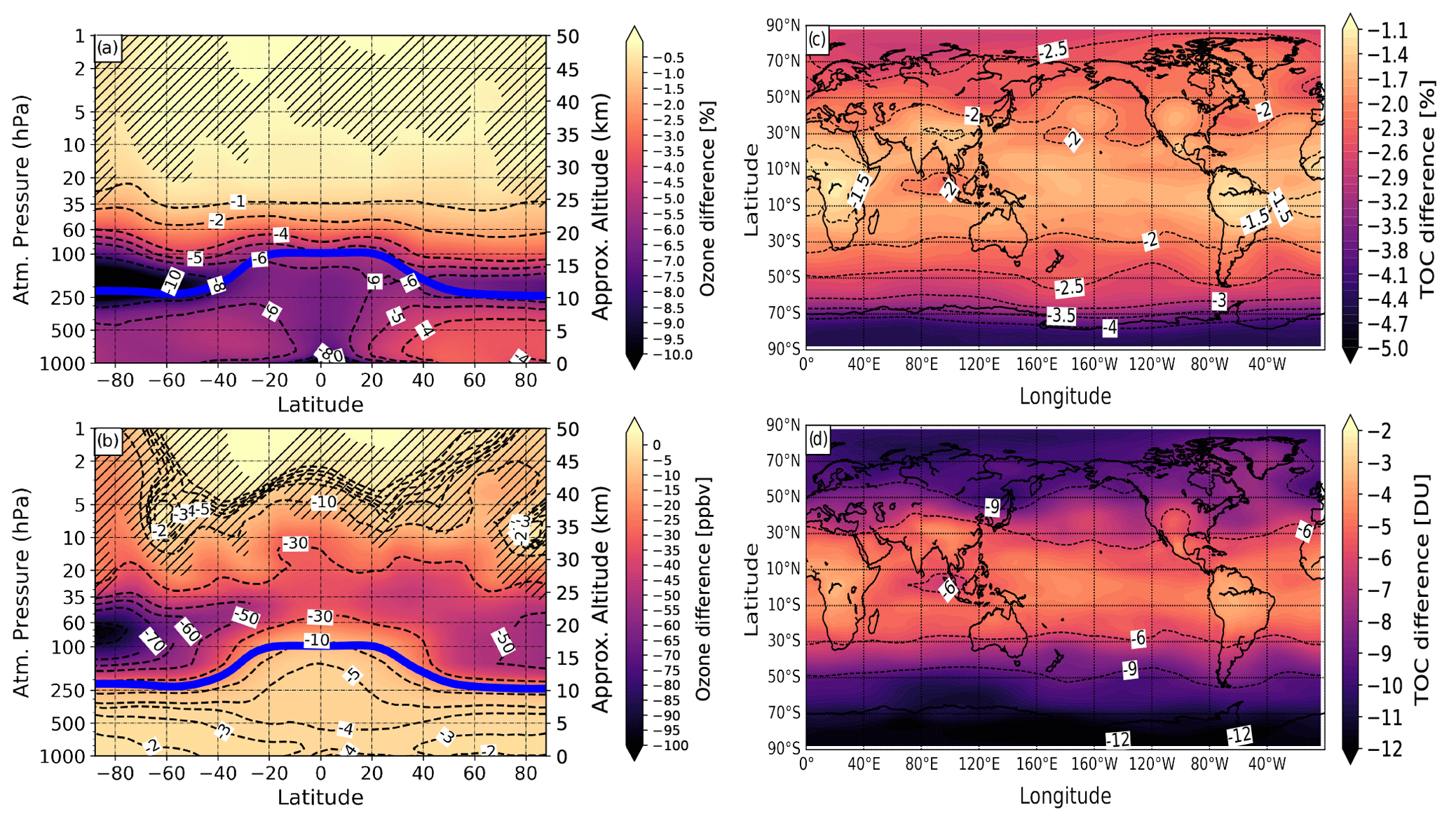
Figure 6 Modeled effect of iodine chemistry on annual-mean ozone climatology averaged for the 2000–2009 period and 10 ensemble members. (a, c) Ozone changes of the case with present-day iodine emissions (1 × iodine) relative to the control run (0 × iodine), presented as zonal mean ozone mixing ratios and total ozone columns (TOC) in percent. (b, d) Corresponding absolute ozone changes in parts per billion by volume (ppbv) and Dobson units (DU), respectively. Blue solid line in (a) and (b): annual mean tropopause height. Hatching marks regions with iodine effect on ozone having a confidence level less than 95 %.

The relative and absolute responses of ozone to iodine chemistry activation are shown for both the ozone mixing ratio and total ozone column (TOC). The relative iodine effect on ozone is calculated as follows: $\left(\right(\mathrm{EXP}-\mathrm{REF})/\mathrm{REF})\times \mathrm{100}$, where EXP is the ozone from the experiment with 1 × loading of iodine and REF is the control run without iodine being included. The absolute difference is simply defined as EXP-REF. The crisp iodine signal in the ozone mixing ratio is observed in the lower stratosphere and intensifies over the polar regions where the effect of halogens is estimated to be higher (Chipperfield et al., 2018). The peak of ozone loss resides in the lower stratosphere over the high southern latitudes, where the ozone loss reaches about 10 % or 100 ppbv. The hemispheric asymmetry of the effect over high latitudes might be caused by a difference not only in the IO_x mixing ratio but also in the mixing ratio of chlorine and bromine in active form (ClO and BrO) that in turn react with iodine. The effectiveness of iodine also depends upon the coupling with chlorine and bromine chemistry intensifying their ozone depletion cycles in the lower stratosphere (see chemical reactions in Table 3). There is evidence that cross-cycles between bromine and chlorine are the dominant contribution to ozone reduction in the mid-latitudes and polar regions (Fernandez et al., 2017; Barrera et al., 2020). The active iodine in the form of IO is also an effective reaction partner for BrO+ClO as established by Read et al. (2008). Thompson et al. (2015) assumed that the interaction of IO with BrO and ClO might be more effective over high latitudes because of their higher concentration in that region (Sioris et al., 2006).

To verify whether or not cross-reactions of iodine with bromine and chlorine largely contribute to the total iodine effect on ozone, we performed an additional experiment where we set the reaction coefficients of all chemical reactions of iodine with chlorine (I-Cl) and bromine (I-Br) to zero. The contribution of iodine chemistry to present-day ozone climatology excluding I-Cl and I-Br cross-reactions estimated by the SOCOL-AERv2-I is presented in Fig. 7.

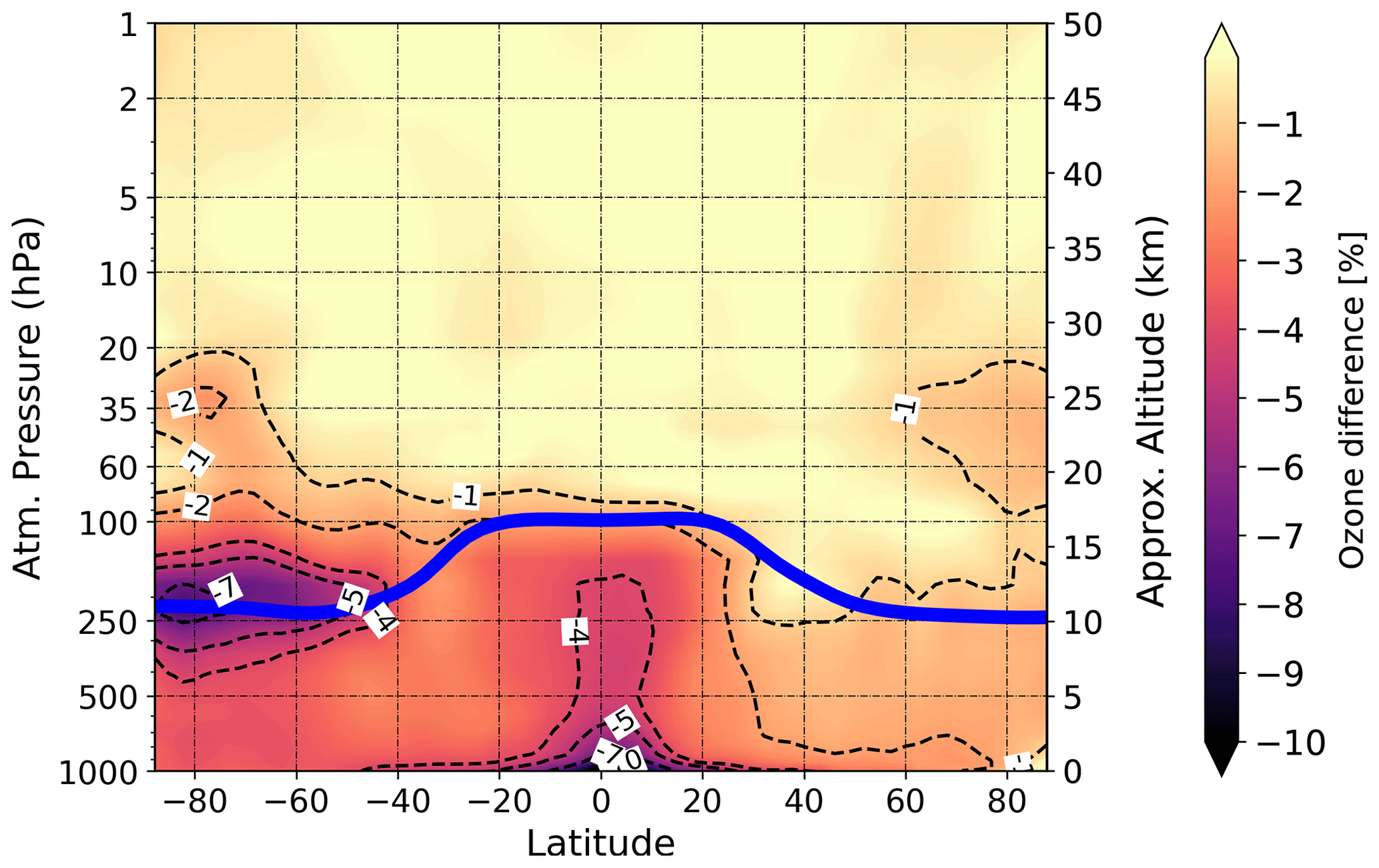
Figure 7 Modeled effect of iodine chemistry on annual-mean ozone climatology excluding I-Cl and I-Br cross-halogen reactions, averaged for the 2000–2009 period. Presented ozone changes of the case with present-day iodine emissions (1 × iodine) relative to the control run (0 × iodine). Blue solid line: annual mean tropopause height.

Comparing Figs. 6a and 7, one can say that the inter-halogen cross-reactions are minor contributors to tropospheric ozone responsible for only about 20 % of total iodine-induced ozone loss. However, in the lower stratosphere, the contribution of these cross-cycles is much higher, covering the 60 %–70 % of total iodine effect on ozone in the Northern Hemisphere. In the Southern Hemisphere, the contribution is found to be less than ∼30 %. Thus, our model suggests that cross-cycles of I with Cl and Br might largely affect ozone and be responsible for more than a half of total iodine-induced ozone reduction in the lower stratosphere, which agrees with Fernandez et al. (2017) and Barrera et al. (2020).

The iodine-mediated ozone loss in the tropical lower stratosphere ranged between 4 %–5 % or 20 ppbv below 20 km. The ozone destruction caused by iodine chemistry is not so pronounced over the tropics because the extremely low temperature in the cold trap on the tropical tropopause that resulted from adiabatic cooling is even lower than the temperature over high latitudes at the same height making catalytic cycles less effective.

It is important to mention that the effects of iodine chemistry are confined mostly to the lower stratosphere and are greatly decreasing from the middle to the upper stratosphere. The “glasses-like” iodine effect in the upper stratosphere similar to the one of ClO_x cycle (Zubov et al., 2013) is not observed. The IO_x-catalytic cycle is ineffective in the upper stratosphere similarly to BrO_x cycle despite the presence of atomic iodine up there in reasonable concentrations. It might be because iodine reservoirs are much more unstable than those of chlorine and, similarly to bromine, the iodine species in lower altitudes will be more likely in active form (IO) than that of chlorine will be in the form of ClO (Daniel et al., 1999). So, the probability of the terminal reaction ClO+O is higher than those of IO+O or BrO+O in the upper stratosphere. It should be noted that SOCOL-AERv2-I demonstrates the decrease in the IO mixing ratio in the upper stratosphere (see Fig. 3b). Hence, the effect of iodine chemistry on upper stratospheric ozone loss is negligibly small.

The tropospheric effect is ∼4–5 ppbv and maximizes over the tropics where iodine sources are mostly emitted from the ocean thanks to its higher temperature. About 6 %–8 % of tropospheric ozone loss is comparable to what was reported by Sherwen et al. (2016a), but surface iodine emissions were a bit higher. It is also in agreement with an estimation made by Davis et al. (1996). Tropospheric ozone loss in SOCOL-AERv2-I is a bit higher than in CAM-chem where the iodine-induced ozone loss does not exceed 2–3 ppbv (Saiz-Lopez et al., 2014).

The total ozone column (TOC) is affected by iodine mostly over high latitudes (see Fig. 6c and d). The highest impact of iodine on climatological TOC is over high latitudes of the Southern Hemisphere showing the TOC loss of about 4 % or 11–12 DU. Over the Northern Hemisphere, the iodine effect on TOC does not exceed 3 %.

3.3 Ozone response to the increased iodine emissions

To estimate the consequences for ozone from the continuous increase in iodine emissions, we compare ozone from the experiment with doubled emissions to that from the experiment with observed (or present-day) emissions. The results are shown in Fig. 8.

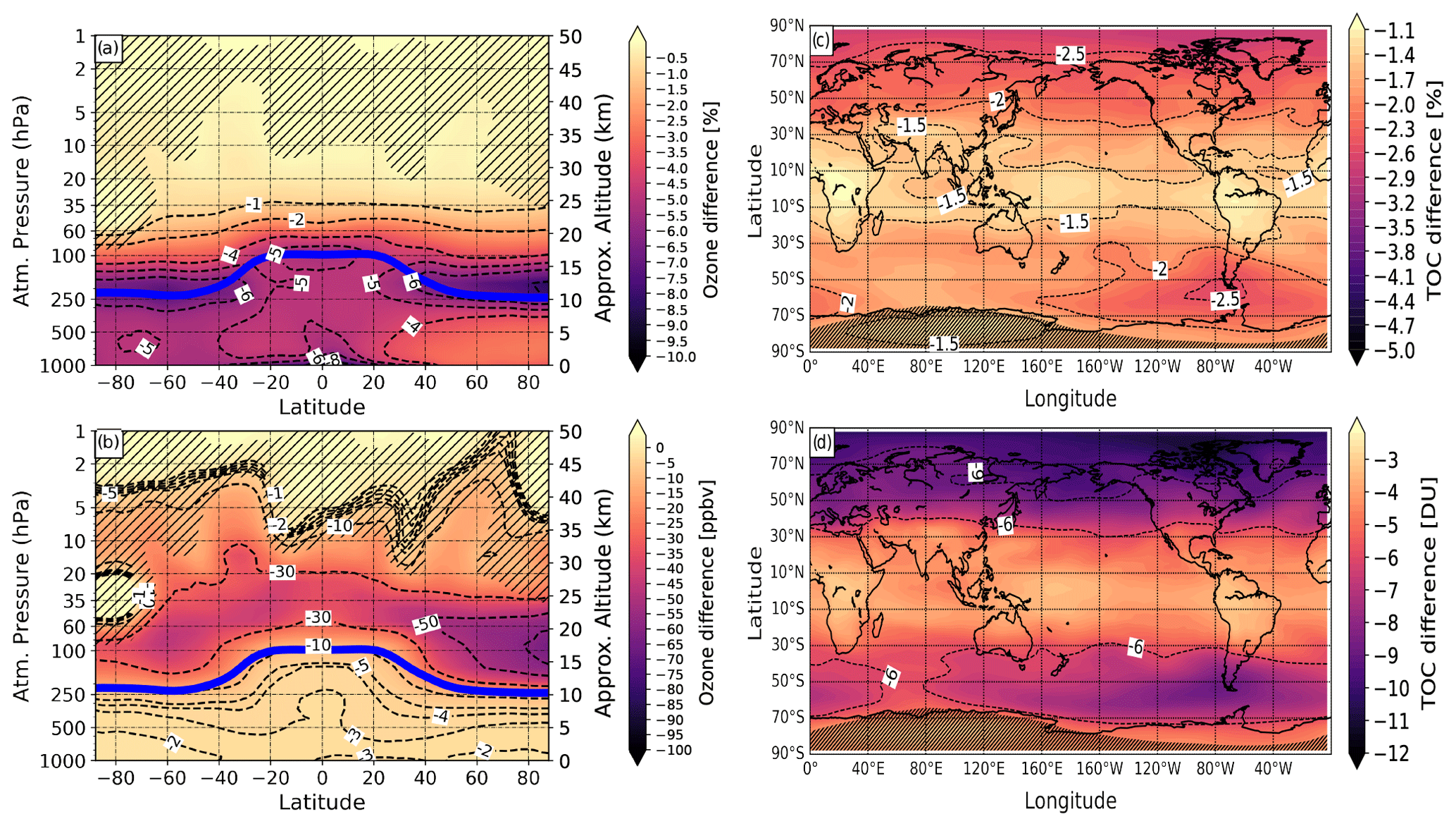
Figure 8 Modeled effect of 2-fold iodine chemistry on annual-mean ozone climatology averaged for the 2000–2009 period and 10 ensemble members. (a, c) Ozone changes of the case with 2-fold iodine chemistry (2 × iodine) relative to present-day iodine emissions (1 × iodine) in percent. (b, d) Corresponding absolute ozone changes in parts per billion by volume (ppbv) and Dobson units (DU), respectively. Blue solid line in (a) and (b): annual mean tropopause height. Hatching marks regions with iodine effect on ozone having a confidence level less than 95 %.

In this case, the EXP was taken to be the experiment with 2 × loading of iodine whereas the REF is the one with observed (1 ×) iodine emissions. In the troposphere, a 2-fold increase in emissions leads to the ozone loss of about 6 %–8 %, which is similar to what is seen in Fig. 6. In the stratosphere, the contribution of additional iodine is different. The southern hemispheric maximum is weakened and shifted to the middle latitude showing the ozone loss of up to 7 % or 50 ppbv. The iodine contribution to ozone loss in the lowermost northern polar stratosphere also shows a similar pattern and magnitude of the effect on the climatology in Fig. 6, showing about 50 ppb of ozone loss. For the Northern Hemisphere, the effect might be characterized as a linear kind too and the intensification of ozone loss by a factor of 2 can be expected. The iodine-induced total column ozone loss would enhance by 2 %–3 % following the 2-fold increase in iodine emissions.

Thus, we can expect that a 2-fold increase in iodine injection into the atmosphere would lead to a mostly linear increase in the ozone loss over the troposphere and lower stratosphere. The reason why we do not see the linearly changed effect over the Southern Hemisphere is possibly related to the saturation effect when the ozone was almost destroyed even for smaller iodine loading. Hence, it can be predicted that the iodine effect on ozone in the lower atmosphere, if the assumed negative iodine scenario plays out in the future, would simply hinge on a factor of the increasing iodine injection into the atmosphere.

3.4 Ozone response to organic and inorganic iodine sources

We also address the effect of organic vs inorganic iodine sources on tropical ozone. To do this, we repeated the experiment with observed (or present-day) emissions twice, setting either organic or inorganic surface emissions to zero. The results are shown in Fig. 9.

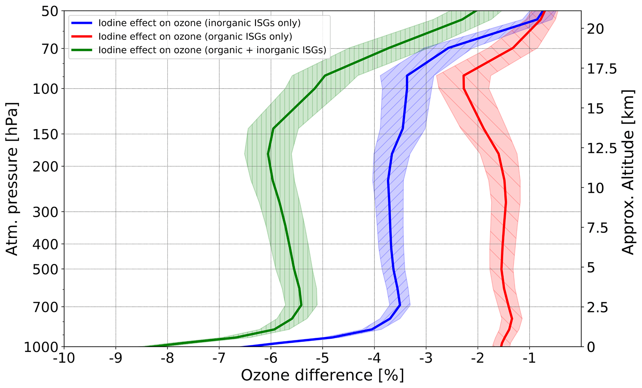
Figure 9 Modeled vertical profiles of O₃ reduction by iodine from organic, inorganic, and total surface emissions averaged over the tropics (20^∘ N–20^∘ S), for the 2000–2009 period and 10 ensemble members. Red curve: difference in O₃ relative to the control run (0 × iodine), if only organic iodine source gases are considered; blue curve: a percentage difference in O₃ relative to the control run (0 × iodine), if inorganic iodine source gases are only considered; green curve: a percentage difference in O₃ relative to the control run (0 × iodine), if both organic and inorganic iodine source gases are considered. Shadings represent a standard deviation of ensemble members. The results have a confidence level more than or equal to 95 %.

In the lower troposphere, the iodine from inorganic emissions is responsible for ∼75 % of total iodine effect on ozone, and the contribution of iodine from organic sources is ∼25 %, as expected (Koenig et al., 2020). In the upper troposphere and lower stratosphere, the ozone responses to iodine from both kinds of sources are closer, but still the impact of inorganic sources prevails, i.e., ∼60 % and ∼40 %, correspondingly. At 50 hPa, the contributions of iodine originating from organic and inorganic sources to total iodine-induced ozone reduction are compatible.

4 Discussion and conclusions

In this study, we describe the new version of the chemistry–climate model SOCOL-AERv2 improved with the addition of the iodine chemistry module. The iodine chemistry scheme in SOCOL-AERv2-I was developed based on up-to-date knowledge about atmospheric iodine. We performed a set of numerical experiments to test the fidelity of the developed iodine chemistry scheme and to estimate iodine contribution to ozone depletion. The model results show about 0.75 pptv of iodine in the lowermost tropical stratosphere in agreement with previous estimations (Saiz-Lopez et al., 2015). A gradual increase in I_y up to 1.05 pptv in the stratosphere might be related to the dynamical features, the effect of tropospheric sinks and/or recycling, or the rigid upper border in the model atmosphere. The comparison of modeled and observed IO within the tropical troposphere showed that IO from SOCOL-AERv2-I is in a generally good agreement with AMAX-DOAS observations. The additional comparison of total gas-phase inorganic I_y with the values determined by the CU box model based on AMAX-DOAS observations of IO showed that the model reproduces the I_y in the upper troposphere very well, while in the stratosphere, I_y is much overestimated due to the absence of simulated iodine in the particulate phase. If the assumed particulate iodine was excluded from the modeled stratospheric I_y, SOCOL-AERv2-I corresponds well with I_y from the CU box model. The simulation of particulate iodine is a subject for future studies as the mechanism of its formation is still not fully understood due to a lack of measurements.

The estimated contribution of iodine chemistry on the lower stratospheric ozone is higher than those discussed in Hossaini et al. (2015), showing up to 10 % of the lower stratospheric ozone loss driven by iodine chemistry. It should be noted that Hossaini et al. (2015) reported only 0.15 pptv of I_y injected into the stratosphere, which is more than 5 times less than in SOCOL-AERv2-I and CAM-chem. In the lower troposphere, the share of ozone loss induced by iodine originating only from inorganic sources is estimated to be 75 %; it is estimated to be 25 % if considering only organic sources. At 50 hPa, contributions of iodine from organic and inorganic sources to total iodine-induced ozone loss are found to be compatible. We also verified that even if the concentration of iodine is much less than other halogens it could play a noticeable role in the lower stratospheric ozone depletion especially over high latitudes. Nevertheless, negative lower stratospheric changes recently found by Ball et al. (2018) might be driven by iodine chemistry only in the lowermost stratosphere as the iodine effect in the extratropical lower stratosphere is not supposed to produce such a broad signal. At the same time, SOCOL-AERv2-I suggests that cross-cycles of iodine with bromine and chlorine might sufficiently affect ozone covering the 50 %–70 % of total iodine contribution to ozone reduction in the lower stratosphere at mid-to-high latitudes with the strongest contribution in the Northern Hemisphere. It should be noted that the $\mathrm{I}-\mathrm{Br}/\mathrm{I}-\mathrm{Cl}$ ratio in the total effect of iodine on ozone requires additional studying. The upper stratospheric ozone is not affected by iodine chemistry, similar to the impact of bromine chemistry, as presumably the iodine species in the upper stratosphere are hardly in more active form (IO) than that of chlorine due to longer lifetime of chlorine precursors (Daniel et al., 1999). Our results also demonstrate a lowering of the IO mixing ratio in the upper stratosphere. Hence, the net effect is that iodine is relatively more important in the lower stratosphere although the abundance of total inorganic gas-phase iodine is expected to be similar throughout the stratosphere (see Fig. 3).

Also, we would like to address here some shortcomings of the current iodine scheme and further updates that are anticipated to increase the accuracy of iodine simulations in chemistry–climate models. A strong local decrease in free tropospheric ozone can be expected from iodine collected inside iodized aerosol particles from deserts and oceans which can reach the above-cloud troposphere where they release iodine (Volkamer et al., 2021). However, such complex aerosol iodine chemistry cannot be properly simulated with current chemistry–climate models (Baker, 2004; Sherwen et al., 2016b). The recent studies of Gómez-Martín et al. (2020), Baccarini et al. (2020), and He et al. (2021) suggested that iodine species can make new aerosol particles that are big enough to be cloud condensation nuclei (CCNs). Polar ice-melting in turn leads to the increase in the atmospheric amount of iodine (Cuevas et al., 2018) which may enhance the formation of CCNs. These findings are worth studying further using global climate models with advanced aerosol chemistry and cloud microphysics. Additionally, higher iodine oxide species presented in our study by I₂O₂, I₂O₃, and I₂O₄ might decompose to form iodine oxoacids that grow further to become CCNs (McFiggans et al., 2004; Burkholder et al., 2004; Saunders et al., 2010). However, the formation of iodine oxoacids is still an open question that needs further study (He et al., 2021). Here, we did not consider any iodine in aerosol form, and these species are represented only in the gas phase. Also, as was mentioned above, in this work we used a simplified approach for photolysis of higher-order iodine oxides. However, the cross sections for photolysis of these species are recently measured and can be used to increase the accuracy of simulation (Lewis et al., 2020). Recent field evidence indicates that the recycling of iodine on sea-salt aerosol, and perhaps other types of aerosols, may be much faster than currently represented (Tham et al., 2021). Also, we did not include CF₃I that also could modify the total concentration of iodine in the atmosphere. However, based on the recent studies, it will not substantially impact the stratospheric ozone loss, showing even less impact than that of CH₃I (Zhang et al., 2020), and will mostly affect the tropical and northern mid-latitude tropospheric ozone because of higher concentrations of pollutants (Youn et al., 2010). All organic iodine emissions in our scheme are prescribed. However, they can be interactively calculated in the model utilizing ocean biogenic sources (Ordóñez et al., 2012). It can also be embodied in the next-generation Earth system model where the ocean biosphere is interactively calculated. As was mentioned above, the sea-surface iodide that is the precursor for HOI $/$ I₂ fluxes has some uncertainty in the models and observations (Chance et al., 2014; Sherwen et al., 2019). However, Shaw and Carpenter (2013) argued that the iodide field does not necessarily solve any uncertainty in the HOI $/$ I₂ flux calculation or other impacts on these fluxes. Nonetheless, there is a prediction for increased iodide that will potentially impact the iodine abundance in the future (Carpenter et al., 2021). Also, there are region-specific parameterizations for sea surface iodide concentration that can be implemented in the next version of the iodine scheme in SOCOL-AERv2-I to increase the reliability of abiotic iodine emissions (Inamdar et al., 2020). Recent investigations of the chemical basis of the HOI $/$ I₂ source can help improve the generalization of empirical source functions (Moreno et al., 2020).

Our sensitivity study showed that the contribution of increased iodine to ozone is almost linear compared to the present-day iodine. To simulate the reliable future impact of iodine on ozone, the recent estimations on future iodine emissions based on RCP scenarios can be used (Iglesias-Suarez et al., 2020). Tropospheric ozone content in SOCOL-AERv2-I is overestimated compared to other models (Revell et al., 2018), which affects the sea-surface deposition of O₃ and its concentration inside the marine boundary layer; hence the accuracy of simulated iodine emissions. There are plans to fix this problem in future versions of SOCOL.

One of the most controversial parts of atmospheric iodine studies is the scrutiny of the role of volcanic iodine in stratospheric chemistry and its effect on ozone. The volcanic iodine impact is worth studying since some of the powerful volcanoes are supposedly capable of directly injecting the iodine into the stratosphere and supposing to result in negative and long-lasting implications for the ozone layer (Bureau et al., 2000; Aiuppa et al., 2005; Balcone-Boissard et al., 2010; Cadoux et al., 2015). However, there is no solid evidence that volcanoes can inject a sufficient amount of iodine into the atmosphere (Schönhardt et al., 2017), and it is needed to organize the measurement campaigns to make estimations of emitted volcanic iodine in a more precise way. The results of this work showed the highest impact of iodine on ozone in the lowermost stratosphere at high latitudes. This finding indicates the necessity of having broad measurements of iodine species in this region.

We also stress that the iodine can presumably be more noteworthy in the future. The intensified Brewer–Dobson circulation might bring more iodine into the stratosphere in the future than today. Also, the further increase in sea surface temperature due to global warming, near-surface ozone, and sea surface iodide concentrations could be the reason for the intensification of iodine emissions in the future, making the atmospheric amount of iodine vastly higher (Cuevas et al., 2018; Legrand et al., 2018; Koenig et al., 2020; Iglesias-Suarez et al., 2020; Carpenter et al., 2021). The effectiveness of iodine for ozone destruction is found to be stable in future warming scenarios and therefore its relative importance increases relative to the other halogens (Klobas et al., 2021).

All of this inspires further efforts to better characterize the iodine in the atmosphere and its impact on ozone loss.

Alongside the further improvements of iodine chemistry simulations in chemistry–climate models, it is necessary to overcome the scarcity of global measurements of iodine chemistry especially in the upper troposphere and lower stratosphere to increase the accuracy of estimations for iodine impact on ozone loss and to make better predictions of the future ozone evolution.