the Creative Commons Attribution 4.0 License.
the Creative Commons Attribution 4.0 License.
 | 28 Oct 2021
Parallel gridded simulation framework for DSSAT-CSM (version 4.7.5.21) using MPI and NetCDF
Phillip D. Alderman
The Decision Support System for Agrotechnology Transfer Cropping Systems Model (DSSAT-CSM) is a widely used crop modeling system that has been integrated into large-scale modeling frameworks. Existing frameworks generate spatially explicit simulated outputs at grid points through an inefficient process of translation from binary spatially referenced inputs to point-specific text input files, followed by translation and aggregation back from point-specific text output files to binary spatially referenced outputs. The main objective of this paper was to document the design and implementation of a parallel gridded simulation framework for DSSAT-CSM. A secondary objective was to provide preliminary analysis of execution time and scaling of the new parallel gridded framework. The parallel gridded framework includes improved code for model-internal data transfer, gridded input–output with the Network Common Data Form (NetCDF) library, and parallelization of simulations using the Message Passing Interface (MPI). Validation simulations with the DSSAT-CSM-CROPSIM-CERES-Wheat model revealed subtle discrepancies in simulated yield due to the rounding of soil parameters in the input routines of the standard DSSAT-CSM. Utilizing NetCDF for direct input–output produced a 3.7- to 4-fold reduction in execution time compared to R- and text-based input–output. Parallelization improved execution time for both versions with between 12.2- (standard version) and 13.4-fold (parallel gridded version) speed-up when comparing 1 to 16 compute cores. Estimates of parallelization of computation ranged between 99.2 % (standard version) and 97.3 % (parallel gridded version), indicating potential for scaling to higher numbers of compute cores.
- Article
(1506 KB) - Full-text XML
- BibTeX
- EndNote


The Decision Support System for Agrotechnology Transfer Cropping Systems Model (DSSAT-CSM; Jones et al., 2003; Hoogenboom et al., 2019) is a widely used crop modeling system with cumulatively more than 14 000 users worldwide since its inception (DSSAT Foundation, 2019) and 13 625 downloads of version 4.7.5 across 179 countries since November 2017 (Gerrit Hoogenboom, personal communication, 5 August 2021). Traditional applications of this system have involved field-scale simulations of agricultural experiments across varied agroclimatic conditions. However, it is increasingly being integrated into large-scale modeling frameworks such as the International Model for Policy Analysis of Agricultural Commodities and Trade (IMPACT; Robinson et al., 2015) developed by the International Food Policy Research Institute and the parallel system for integrating impact models and sectors (pSIMS; Elliott et al., 2014). The key interest in these applications is providing gridded inputs (i.e., input data across a grid of spatially referenced points) to a model and receiving back from the model corresponding gridded outputs (i.e., spatially explicit simulated outputs at the same grid points). At the core of these frameworks is a process of translation from binary spatially referenced inputs to point-specific DSSAT-format text input files, followed by translation and aggregation back from point-specific DSSAT-format text output files to binary spatially referenced outputs. File input–output operations are widely known to increase execution time, and conversion from floating point to text and back is inefficient from memory use and computation perspectives. Thus, the conversion from spatial format to point-specific text inputs and from point-specific text outputs to spatial format presents a bottleneck for large-scale simulations. Heretofore, this bottleneck has been overcome largely by use of high-performance computing (HPC) clusters or cloud computing resources, while comparatively little effort has been invested in improving the efficiency of the I/O process. Designing flexible parallel gridded input–output libraries for DSSAT-CSM would improve the computational efficiency and reduce execution time, thereby allowing more efficient utilization of available computing resources.
As noted by Kang et al. (2015) and Jang et al. (2019), examples of improving execution time for agricultural system models being applied at large scales using HPC are limited. Nevertheless, considerable increases in speed of execution have been documented in some models by leveraging parallel execution and linking to gridded input–output libraries. For example, Nichols et al. (2011) found a 40-fold speed-up of simulations by porting the Erosion Productivity Impact Calculator (EPIC) model from Windows to Linux and parallelizing simulations (i.e., running multiple instances of a model simultaneously) on an HPC cluster. Subsequent improvements using the Message Passing Interface (MPI) have permitted up to 512-fold speed-up of EPIC simulations (using 2048 parallel processes) with nearly linear scaling up to 128 parallel processes (Kang et al., 2015). Zhao et al. (2013) reported an average 20-fold speed-up on multi-core Windows computers while running the Agricultural Production Systems Simulator (APSIM) model using the HT Condor grid computing middleware. Much like the IMPACT and pSIMS frameworks described above, all of these studies relied on text-based input and output. In contrast, Vital et al. (2013) avoided use of text input files by linking the PaSim grassland model with the Network Common Data Form (NetCDF) library (Unidata, 2017) for reading and writing gridded data files. They reported up to 200-fold speed-up with nearly linear scaling of parallelized pasture simulations using MPI with up to 200 parallel processes. It was hypothesized that implementing a parallel gridded simulation framework for DSSAT-CSM (i.e., one that runs simulations in parallel and reads and writes directly from and to gridded input–output files) would permit performance gains similar to those reported by Vital et al. (2013). Thus, the main objective of this paper was to document the design and implementation of a parallel gridded simulation framework for DSSAT-CSM. A secondary objective was to provide preliminary analysis of execution time and scaling of the new parallel gridded framework.
Descriptions of the DSSAT-CSM and of the submodules contained therein
have been published elsewhere (Jones et al., 2003), and the code for the
current release version of the standard DSSAT-CSM is now open-source and
can be found at https://github.com/DSSAT/dssat-csm-os/tree/master (last access: 27 October 2021).
Thus, the description here will focus on modifications that were made to
the standard version to facilitate efficient parallelization and gridded
input and output. The specific version of source code documented in this
paper can be found at the following DOI: https://doi.org/10.5281/zenodo.4893438 (Porter et al., 2021). The current version of source code can be found in the gridded
branch of a fork from the official DSSAT-CSM repository
(https://github.com/palderman/dssat-csm-os/tree/gridded, last access: 27 October 2021). These
modifications can be grouped in terms of internal data transfer, gridded
I/O, and parallelization of simulations. A description of the required
NetCDF file structures is also provided in this section.
2.1 Internal data transfer
The first category of code changes for DSSAT-CSM were made to support
more efficient transfer of data between the internal components of
DSSAT-CSM. In the standard open-source version (OS), the code from input
subroutines reads data needed for simulation from files (e.g., crop
management details, cultivar parameters, and soil input data) and writes
these data into a consolidated input file (either DSSAT47.INP or
DSSAT47.INH depending on the crop model being used for simulations). The
subsequent crop and soil modules then read the consolidated input file
to access the required input data. The process is illustrated in the
OS-labeled portion of Fig. 1. This procedure is a
holdover from legacy code developed when the input routine existed as a
separate executable run prior to calling crop and soil models. The input
routine was subsequently merged with the main DSSAT-CSM executable code,
but, as of version 4.7.5.21, the overall structure of the input
subroutines remains largely unchanged. Additionally, this legacy code
makes use of COMMON blocks for sharing data between subroutines
within the input code. These COMMON blocks are now generally
considered poor programming practice due to the ease with which data can
be unintentionally corrupted if used improperly.

Figure 1Flowchart illustrating the data transfer processes implemented in the standard open-source (OS) and parallel gridded (PG) versions of the Decision Support System for Agrotechnology Transfer Cropping Systems Model. The folder shape indicates a step that involves reading or writing a file. The cylinder shape indicates an in-memory data structure.
Consequently, a Fortran module (csm_io) implementing a
flexible data structure and associated functions and subroutines was
developed to replace the consolidated input file and provide a
structured way of transferring data between subroutines that does not
rely on the use of COMMON blocks. The parallel gridded (PG)
version documented herein utilizes this in-memory data structure in
place of the intermediate files used by the OS version (i.e., DSSAT47.INP
or DSSAT47.INH), as illustrated in the PG-labeled portion of Fig. 1. Code implementing the new csm_io module is
in the csm_io.f90 source file at
https://github.com/palderman/dssat-csm-os/tree/gridded/FlexibleIO (last access: 27 October 2021).
An example program that illustrates the use of the csm_io
module is given in Appendix A. This example program
sets the value for three variables of types real, integer, and
character. The type-bound subroutine csminp%add_sec() is used
to add a new section to the data structure, and the type-bound
subroutine csminp%add_var() is used to add entries for the
three variables. The type-bound subroutine csminp%put() is
used to store the current values for the three variables. Finally, the
type-bound subroutine csminp%get() is used to retrieve the
stored values for each of the three variables. In addition to scalar
values, the structure can also handle 1-D arrays of real,
integer, and character types. In the PG version of DSSAT-CSM, the
csm_io module was used to replace subroutines
OPTEMPXY2K() and OPTEMPY2K(), all use of
COMMON blocks, and all code that relied on writing to or
reading from DSSAT47.INP or DSSAT47.INH. This resulted in modifications
to the main CSM program as well as modifications to a number of
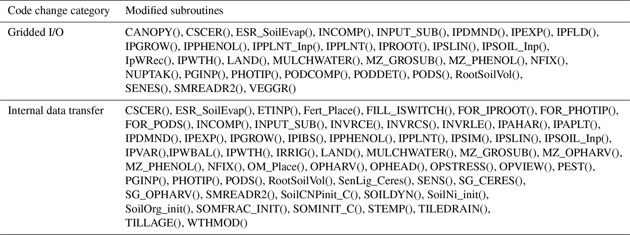
subroutines, each of which is listed in Table 1.
Table 1Subroutines modified in the development of the parallel gridded version (PG) of the Decision Support System for Agrotechnology Transfer Cropping Systems Model (DSSAT-CSM). Subroutines are listed according to category of code change: internal data transfer, gridded input and output (gridded I/O).
2.2 Gridded input and output
Gridded input and output for the PG version of DSSAT-CSM relies on an
interface to Network Common Data Form (NetCDF), which is a set of software
libraries that define self-describing, portable data formats that
support the creation, access, and sharing of array-oriented scientific
data (Unidata, 2017). The DSSAT-CSM NetCDF interface is defined in two
Fortran modules: nf90_file_module and dssat_netcdf.
The nf90_file_module provides a derived type for NetCDF files
that contains type-dependent low-level utility functions and/or subroutines for
creating and manipulating NetCDF files including reading and writing
scalar and array variables of real, integer, and character types. The
dssat_netcdf module provides extensions to this basic derived
type and associated type-dependent utility functions and/or subroutines that
are specific to the various types of input files required for DSSAT-CSM.
Thus, the dssat_netcdf operates as a higher-level interface
that DSSAT-CSM model developers would interact with, while leaving the
more mundane details of communicating with the NetCDF libraries to be
handled by the nf90_file_module.
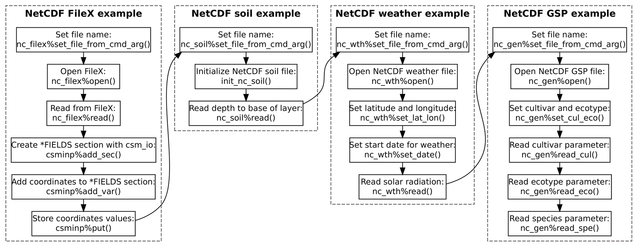
An example program using the dssat_netcdf module to read
DSSAT-CSM FileX, soil, weather, and genotype-specific parameter inputs
from NetCDF files is given in Appendix B and is
illustrated visually in Fig. 2. This example
program also makes use of several other Fortran modules that implement a
data structure (ordered_array) that stores its elements in
increasing order, various utility functions and subroutines related to
reading command-line arguments (dssat_cmd_arg), the
csm_io module (discussed in Sect. 2.1), and the
dssat_mpi module (discussed in Sect. 2.3). The
program begins with several operations related to reading the NetCDF
version of the FileX. For readers less familiar with DSSAT-CSM
terminology, the FileX is a file type that contains information about
various aspects of crop management as well as configuration options for
running simulations. The first operation in the program sets the file
name for the NetCDF FileX by calling the type-bound subroutine
nc_filex%set_file_from_cmd_arg(). This subroutine bound
to the nc_filex variable, which is of derived type
nf90_file (defined in the nf90_file_module),
searches for a command-line argument matching the provided flag
--nc_filex (e.g., --nc_filex=filex.nc) and reads
the associated file path and name. Command-line arguments accessed using
the dssat_cmd_arg module need not be provided in any
particular order but should come after the standard DSSAT command-line
arguments for the run type (e.g., B for batch mode, N
for seasonal mode, Q for sequence mode) and batch file
(typically DSSBatch.V47) in order not to interfere with other
components of DSSAT-CSM that expect these arguments to immediately
follow the executable name. Once the file name is set, the NetCDF FileX
is then opened with the type-bound nc_filex%open(). The
standard FileX format contains multiple “tables” of data stored within
sections of the file and connected via key values or “levels”. Each
row of the TREATMENT table contains a unique combination of key
values that defines a given treatment. Further discussion of the NetCDF
FileX file structure is provided in Sect. 2.4. In the
case of the example program, the value for the 10th row of the
FL column is read into the variable field_level using
the type-bound subroutine nc_filex%read(). This
field_level is then used to read the corresponding values of
XCRD and YCRD from the FIELDS table into the
variables longitude and latitude. The program then
creates a new section (*FIELDS), adds the XCRD and
YCRD as real-type variables, and stores the longitude
and latitude values in the csminp data structure.
Next, the program reads the file name for the NetCDF soil data file from
the command line using the type-bound subroutine
nc_soil%set_file_from_cmd_arg() and calls the
init_nc_soil() subroutine that is defined in the
dssat_netcdf module (Appendix B).
This subroutine retrieves the previously stored values for XCRD
and YCRD from the csminp data structure, opens the
NetCDF soil file, and sets the latitude and longitude coordinates within
the nc_soil variable. These latitude and longitude values are
used to determine the proper coordinates from which to subsequently read
soil variables. The program then reads the array of values for the
variable of the depth to the base of the layer (SLB) starting from index 1 and
stores it in the local 1-D array SLB using the type-bound
subroutine nc_soil%read(). Other scalar and 1-D array
variables can be read using the same call. The NetCDF soil data file
structure is discussed in greater detail in Sect. 2.4.
The example program proceeds by reading the NetCDF weather file by first
setting the file name, opening the NetCDF file, and setting the spatial
coordinates for the grid point (Appendix B).
The start date for reading weather data is then set by calling the
type-bound subroutine nc_wth%set_date(), which sets the
internal index based on the date specified. The date argument is
specified as an integer with the first four digits representing the year and the
last three digits representing the Julian day of the year. This internal index is
then used in subsequent calls to the type-bound subroutine
nc_wth%read() by including the nc_wth%z_i
variable as the starting index value. This is illustrated in the example
program by reading the solar radiation (SRAD) variable. The
NetCDF weather data file structure is addressed in Sect. 2.4.
Following the weather file, an example of reading the NetCDF genotype
parameter file is provided (Appendix B).
Setting the file name and opening the NetCDF file follow the same
procedure as for the other file types. However, instead of setting
latitude and longitude coordinates (as is done for soil and weather
files), the cultivar code is set by calling the type-bound subroutine
nc_gen%set_cul_eco(). Following this call, the cultivar
parameter P1V is read from the file using the type-bound
subroutine nc_gen%read_cul(). Similarly, the ecotype
parameter PARUE is read from the file using the type-bound
subroutine nc_gen%read_eco(), and the species parameter
TRLFG is read using the type-bound subroutine
nc_gen%read_spe(). More specifics on the NetCDF genotype
parameter file structure are provided in Sect. 2.4.
In addition to the development of the DSSAT-CSM NetCDF interface,
existing code was modified to ensure compatibility with the new
DSSAT-CSM NetCDF interface. Subroutines modified to use the NetCDF
interface are given in Table 1. In general, the code
changes involved adding an if construct that first checks
command-line flags to determine if the input type (e.g., soil data) is to
be read from the DSSAT standard format or from the NetCDF gridded
format. If the former, the original OS code is executed, while
new code calling the NetCDF interface is executed if the latter
condition is met. Some subroutines were not conducive to simple
modification by use of an if construct and therefore required
implementation of a new version of the subroutine compatible with the
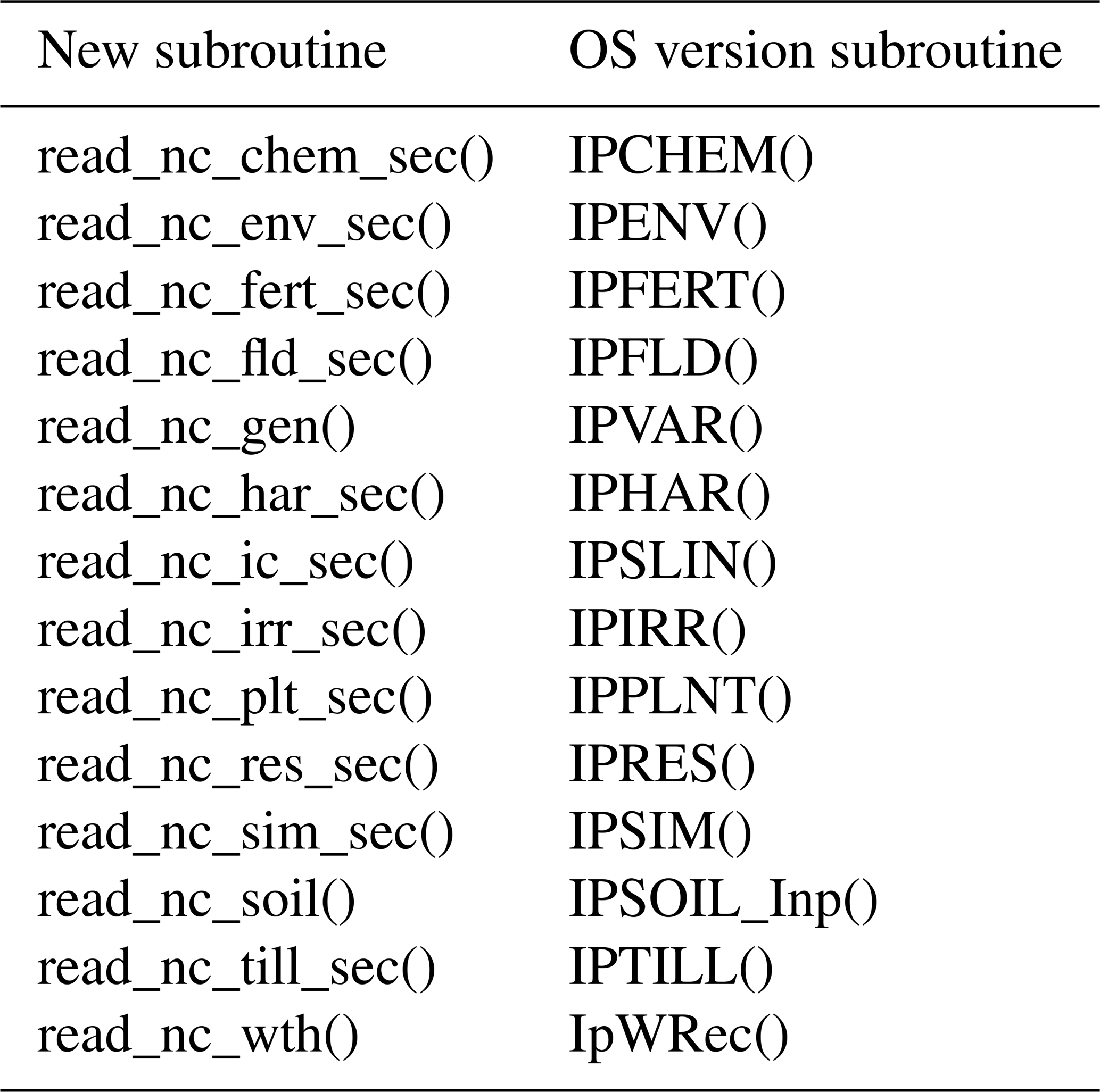
NetCDF interface. A list of these new subroutines and their original OS
version counterparts is given in Table 2. In general, for
each pair of new and OS subroutines an if construct in each
“parent” subroutine checks command-line flags to determine which
subroutine should be called (i.e., either the OS version or the
new NetCDF-compatible one).
Table 2New subroutines created in the development of the parallel gridded version (PG) of the Decision Support System for Agrotechnology Transfer Cropping Systems Model (DSSAT-CSM). New subroutines are listed with the corresponding subroutine from the standard open-source version (OS) of DSSAT-CSM.
2.3 Parallelization
Parallelization for the PG version of DSSAT-CSM relies on the Message Passing Interface (MPI), a widely used specification that follows a message-passing parallel programming model especially suitable for distributed memory systems (Message Passing Interface Forum, 2015). The MPI specification was selected primarily due to its widespread usage and suitability for distributed memory systems (e.g., HPC clusters). Specifically, MPI has been used successfully in other applications for parallelizing crop models (Nichols et al., 2011; Kang et al., 2015; Jang et al., 2019; Vital et al., 2013). The message-passing parallel programming model allows multiple independent DSSAT-CSM instances to run concurrently, each of which manages its own memory and most of its input and output. This approach reduces the number of required modifications to the core DSSAT-CSM model code and thereby eases the burden in maintaining synchronization between the PG version and the model code maintained by the DSSAT core developer team.
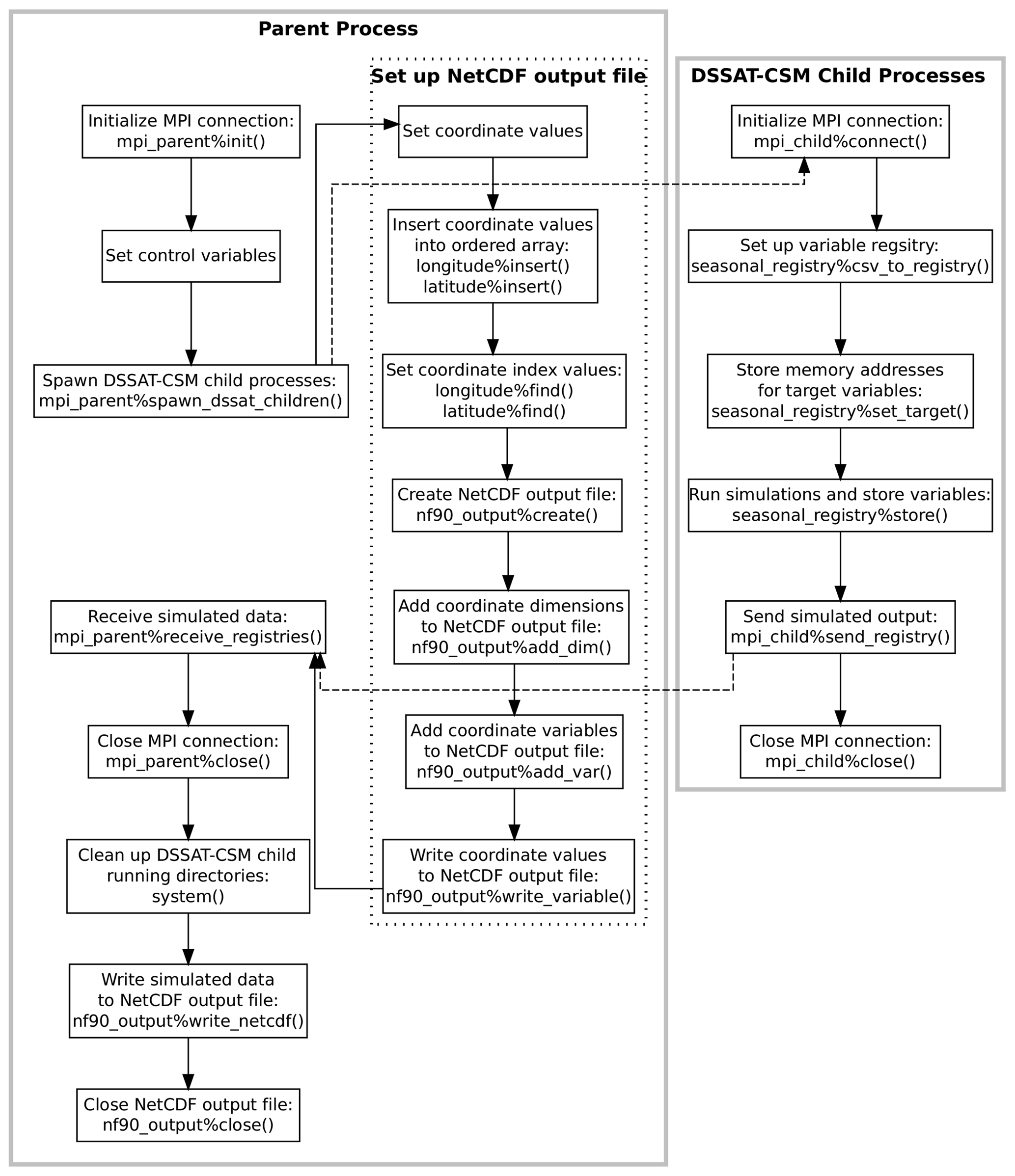
Figure 3Flowchart illustrating the points of communication and sequence of operations for the example parent and child programs given in Appendices C and D and explained in Sect. 2.3. Solid gray borders indicate the boundary of a process. The dotted border indicates a grouping of operations within a given process. Dashed arrows indicate communication between processes using Message Passing Interface (MPI) protocols.
Overall, the DSSAT MPI consists of a Fortran module
(dssat_mpi) and a control program (parent process) that
spawns multiple instances of the DSSAT-CSM (“child” processes),
assigns a range of treatment numbers to each instance, receives
simulated results from each instance, and writes a NetCDF-format output
file. Several changes were made to the DSSAT-CSM main program to open an
MPI connection with the parent process, store simulated output for
subsequent transfer, and transfer simulated output to the parent
process. All communication between the parent process and each spawned
child process is mediated through two derived types defined in the
dssat_mpi module, namely mpi_parent and
mpi_child. An example program illustrating the parent process
is given in Appendix C, and a corresponding example child
process program is given in Appendix D. A visual
illustration of the parent and child processes and communication between
them is provided in Fig. 3. The parent program
begins by defining a comma-delimited list of variables, storing it in
the mpi_parent%varlist variable, and defining an output file
name. The program then calls the type-bound subroutine
mpi_parent%init(), which initiates an MPI connection by
calling MPI_Init() as defined in the MPI specification.
Thereafter, the parent program sets several local variables that are
used to spawn the DSSAT-CSM child processes. In the PG version of
DSSAT-CSM, each of these variables, mpi_parent%varlist, and
the output file name are supplied to the master process program as
command-line arguments. The type-bound subroutine
mpi_parent%spawn_dssat_children() is then called, which
constructs working directory names, command-line arguments, and commands
for each of the children DSSAT-CSM processes and calls
MPI_Comm_spawn_multiple(), which is the MPI specification for
spawning multiple children processes. The command-line flag
--MPI is included in the argument list for each of the
children DSSAT-CSM processes, which signals the executable to
initiate an MPI connection and connect to the parent program. The
mpi_parent%spawn_dssat_children() subroutine also uses
MPI_Send() (the MPI specification for performing a blocking
send) to transfer the treatments assigned to each DSSAT-CSM child
process, the output variable list, the run mode, and the crop code for
simulation. These MPI data transfers are represented by a dashed arrow
in Fig. 3. After sending these data to each child
process, the subroutine allocates an array of data structures (one
element per child process) in which to store the simulated output from
each child process. Each data structure (referred to as a variable
registry) is then initialized using the comma-separated variable list
contained in mpi_parent%varlist.
Appendix D provides an example child process that mimics
the action of a DSSAT-CSM child process in the way in which it interacts
with the parent process. The program begins by connecting to the parent
process by calling the type-bound subroutine
mpi_child%connect(), which calls MPI_Init(),
MPI_Comm_rank(), and MPI_Comm_get_parent() each
once and MPI_Recv() multiple times to receive the elements of
data sent from the parent process. The subroutine then uses the
system() intrinsic subroutine to run the mkdir shell
command with the path for the specific working directory assigned to
that child process. The chdir() intrinsic subroutine is then
called to move the child process into that working directory to begin
running simulations.
The reliance upon the mkdir shell command and the non-standard
GNU GFortran extension chdir() subroutine makes the code less
portable; thus, a few words on the matter are warranted here. Assigning
child processes to their own specific working directories has been
implemented to avoid competition between processes in simultaneously
attempting to write to identical output files. Although most direct
writing of output to text files has been eliminated, occasional messages
are still generated by various components across the DSSAT-CSM and
written to standard files (e.g., WARNING.OUT). With all child
processes running in the same directory, competition for these files can
become problematic. The long-term intention is to eventually account for
these sources of output and remove the need for invoking shell commands
and non-standard subroutines. Nevertheless, because most HPC clusters
run some form of *nix operating system, the shell command strategy
should not be problematic in most use cases. Likewise, the GNU compiler
collection is available in most HPC environments. Users also have the
option of customizing these two lines of code within the
connect_to_parent() subroutine to fit their own compiler and
operating system constraints.
Once the child process has connected with its parent, the child
initializes a variable registry to contain seasonal simulated output by
calling the seasonal_registry%csv_to_registry() with the
mpi_child%varlist argument (Appendix D). This
initializes a variable registry with an entry for each of the variables
listed in mpi_child%varlist. The variable registry data
structure is an instance of the derived type registry_type
defined within the dssat_variable_registry Fortran module. It
is essentially an array of type registered_variable (also
defined in the dssat_variable_registry module), along with
subroutines for initializing the variable list, adding new variables to
the array, associating elements with specific variables, and storing
variable values. The registered_variable type is a derived
type with a character variable component for the variable name,
allocatable array components of real and integer types, pointers of real
and integer types, and subroutines for initializing the variable,
reallocating the variable, and storing values. When each variable is
initialized, the allocatable array component used for storing data is
allocated. If the variable to be stored is of type real, then the real
array is allocated. If the type is integer, then the integer array is
allocated. To store values for a given model variable, one of the
pointers (real or integer depending on the type of the variable) must
also be associated with the address of the variable. In the example
child program this is done by calling the
seasonal_registry%set_target() subroutine first for a real
variable rvar and then for an integer variable ivar
(Appendix D). In the PG version of DSSAT-CSM, the
seasonal_registry%set_target() subroutine is called in each
subroutine wherein a variable of interest is defined. For example, within
the CROPSIM-CERES-Wheat CSCER() subroutine there is a line that
calls
seasonal_registry%set_target('CWAM' ,CWAD),
which associates the memory address of the CWAD state variable
for aboveground biomass with the CWAM name within the variable
registry. Once the addresses for all variables have been stored in the
variable registry, the seasonal_registry%store() subroutine
can be called at each iteration, and the then current value at each of
the associated memory addresses will be stored. An example of this is
shown in Appendix D. Once all simulations are complete,
the variable registry (seasonal_registry) is sent to the
parent process through MPI by calling
mpi_child%send_registry(), and the MPI connection is
terminated by calling mpi_child%close(). These operations are
summarized in the right portion of Fig. 3. The
strategy of storing memory addresses and retrieving values from them at
the end of each seasonal iteration is predicated upon the fact that all
state variables in the DSSAT-CSM are statically allocated by using the
SAVE statement at the beginning of variable declarations in all
subroutines. Thus, the address of state variables is stable within a
given run of the model. Moving away from static allocation of state
variables would require an overhaul of nearly every subroutine in
DSSAT-CSM and is thus unlikely to occur in the foreseeable future.
While the children processes run simulations, the parent program creates
the combined simulation output file (Appendix C). It
first defines dimensions for the NetCDF output file (nseasons,
xcrd and ycrd) that, in the PG version of DSSAT-CSM,
are read from the NetCDF FileX. The name of the FileX is supplied as a
command-line argument. The xcrd and ycrd values are
inserted into ordered arrays (a custom data structure similar to the C++
Standard Template Library ordered set and defined in the module
ordered_array) for longitude and latitude.
The ordered arrays do not contain duplicate values, and the values are
arranged in order from lowest to highest. Because of this the dimension
and order of values in the longitude and latitude
ordered arrays do not match xcrd and ycrd and new
indices for each xcrd and ycrd (xcrd_i and
ycrd_i) must be set based on searching for the corresponding
value for xcrd(i) in longitude and for
ycrd(i) in latitude. Once this process is complete,
the output NetCDF file is created by calling
nf90_output%create() and calling
nf90_output%add_dim(), nf90_output%add_var(), and
nf90_output%write_variable() for each coordinate variable
(lat, lon, and season). These operations are
summarized in the dashed box within the parent process box in Fig. 3. Once the output file is set up, the parent program
calls the mpi_parent%receive_registries() type-bound
subroutine, which listens for transfer of simulated output from the
DSSAT-CSM children processes in the form of a variable registry, as
discussed above.
Once the DSSAT-CSM children processes complete all simulations and the
parent program has received the simulated output, the parent program
closes the MPI connection and invokes the rm shell command
using the system() intrinsic subroutine to remove each of the
directories previously created for the DSSAT-CSM children processes. The
parent program then concludes by calling the type-bound subroutine
nf90_output%write_netcdf() to write the values returned
by the children DSSAT-CSM processes to a single NetCDF output file and
then closing the file.
2.4 Input file conventions
The NetCDF interface described in Sect. 2.2 is unusable without properly formatted input files. Thus, this section will document the file structures required for use with the DSSAT-CSM NetCDF interface. Header information from the example FileX, soil, weather, and genotype-specific parameter input NetCDF files is presented in Appendices E, F, G, and H.
2.4.1 FileX
As previously mentioned, the standard DSSAT FileX format contains
multiple tables of data stored within sections of the file and
connected via key values. In the NetCDF version of the FileX the number
of rows in each table is represented by the corresponding dimension
defined in the file. The tables defined in the NetCDF FileX header given in
Appendix E include SIMULATION CONTROLS,
FIELDS, CULTIVARS, TREATMENTS,
PLANTING DETAILS, FERTILIZERS, and
HARVEST DETAILS. The header also contains dimensions that
correspond to the length of character vectors stored in the file
(e.g., len1, len2, len6). After the
definition of dimensions in the file comes the full list of variables
defined in the file. For each integer- (int) and real-type
(float) variable, the dimension variable corresponds to the
FileX table to which the variable belongs. For each character-type
(char) variable the first dimension denotes the FileX table to
which the variable belongs and the second dimension defines the length
of the character variable. For example, the
SIMULATION CONTROLS dimension in Appendix
E has size 20, indicating that there are 20 rows in the
SIMULATION CONTROLS table. Thus, for the variable
SUMRY the first dimension is
SIMULATION CONTROLS and the second dimension
is len1, indicating that it is a length-1 character variable
in the SIMULATION CONTROLS table (i.e., with 20 values). Similarly, the
FIELDS dimension has size 7208, indicating that the
FIELDS table contains 7208 rows. Thus, the AREA
variable (defined with the FIELDS dimension) is in the
FIELDS table and accordingly contains data for 7208 grid
points (“fields” in FileX parlance).
2.4.2 Soil inputs
The NetCDF soil data file has a much simpler structure with three
dimensions: latitude, longitude, and layer
(Appendix F). The latitude and
longitude dimensions represent the spatial dimensions of the
soil data, with the latitude and longitude variables
containing the coordinate values associated with each grid point. A
third dimension (layer) is defined for use with variables that
contain layer-specific values (i.e., values that vary with soil depth) at
each grid point. For example, the SLB (depth to the base of the layer)
variable is defined with the latitude, longitude, and
layer dimensions because SLB contains layer-specific
values. In contrast, the SALB (soil surface albedo) variable
only contains a single value per grid point and is thus defined with
only the latitude and longitude dimensions. Further
details about these and other variables following the DSSAT standard
nomenclature for soils data are described in the SOIL.CDE file
(available at
https://github.com/palderman/dssat-csm-os/tree/gridded/Data/SOIL.CDE, last access: 27 October 2021).
2.4.3 Weather inputs
The NetCDF weather data file also has a relatively simple structure, with
the latitude and longitude dimensions defined in the
same way as for the NetCDF soil data file (Appendix G). The NetCDF weather file also contains a third
dimension, DATE, which encodes the time dimension of the dataset.
The coordinate values within this dimension are stored as integer type
and follow the internal encoding of the YEARDOY variable within
the DSSAT-CSM; namely, the leftmost four digits encode the
four-digit year and the remaining three digits to the right encode the
Julian day of the year. For example, the value 2020001 would encode 1 January 2020 and the value 2020366 would encode 31 December 2020. Just as
for the soil data, some weather variables have a single value per grid
point (e.g., TAV, average annual temperature) and are defined
with only the latitude and longitude dimensions. Other
variables have daily values at each grid point and are defined with the
latitude, longitude, and DATE dimensions
(e.g., RHUM, average daily relative humidity). Further details
about these and other variables following the DSSAT standard
nomenclature for weather data are described in the WEATHER.CDE file
(available at
https://github.com/palderman/dssat-csm-os/tree/gridded/Data/WEATHER.CDE, last access: 27 October 2021).
2.4.4 Genotype-specific parameters
Finally, the genotype-specific parameter (GSP) NetCDF file structure is
slightly more complex than the NetCDF soil and weather data files
although less so than the FileX. At present, the GSP NetCDF file is the
only NetCDF input file that does not contain any spatial coordinates
(Appendix H). The dimensions of the file are set based on
the number of cultivars and ecotypes included in the file as well as the
dimensions of species parameter arrays. For example, the cultivar
parameter P1V (vernalization requirement) is defined with
dimension l12 (with length 12) because there are 12 cultivars
in the file. Likewise, the ecotype parameter P1 (duration of
phase from end of juvenile to terminal spikelet) is defined with
dimension l11 (with length 11) because there are 11 ecotypes
defined in the file. Finally, PGERM (germination phase
duration) is a species parameter defined with dimension l1
(with length 1) because that parameter is a scalar value, and
LAFS (leaf area senesced; also a species parameter) is defined
with dimension l6 because it contains values for each of 6
growth stages. Cultivar and ecotypes in standard DSSAT format are
specified using a unique six-digit character code for each cultivar and
ecotype. In the NetCDF GSP file these six-digit character codes are
prepended with either CUL (cultivar) or ECO (ecotype) to generate a unique
name for a scalar integer that stores the index value for that
particular cultivar or ecotype. For example, the cultivar code IB0488 is
used for the Newton wheat cultivar, and thus the CULIB0488
variable in the NetCDF GSP file stores the index for the Newton
cultivar. When reading values for the Newton cultivar, the NetCDF
interface uses this index value to retrieve the correct value for any
cultivar parameters (e.g., the fifth value from the P1V array).
Correspondingly, the ECOUSWH01 variable in the NetCDF GSP file
stores the index for the USWH01 ecotype. Because the ecotype associated
with the Newton cultivar is USWH01, the NetCDF interface first reads the
index value from ECOUSWH01 and then uses it to retrieve the
proper value for ecotype parameters (e.g., the fifth value from the
P1 array). Further details and definitions of all cultivar,
ecotype, and species parameters can be found in the WHCER047.CUL,
WHCER047.ECO, and WHCER047.SPE files at
https://github.com/palderman/dssat-csm-os/tree/gridded/Data/Genotype/ (last access: 27 October 2021).
3.1 Software versions
Simulations from three versions of the DSSAT-CSM were compared for
validating the parallel gridded interface described in Sect. 2. The first version was the standard open-source
version 4.7.5.21 of DSSAT-CSM (abbreviated OS;
https://github.com/dssat/dssat-csm-os, last access: 27 October 2021), which uses standard
DSSAT-format text files for input and output. The second version was the
parallel gridded version 4.7.5.21 of DSSAT-CSM (abbreviated PG), which
contains the changes documented in Sect. 2. Initial
comparison of simulated results from the PG and OS versions revealed
discrepancies that will be discussed below (see Sect. 4.1). In order to investigate these
discrepancies, a third version (referred to as PG-MI) was implemented as
an extension from the PG version in order to mimic the way in which the
OS version rounds soil input data when writing the
DSSAT47.INP/DSSAT47.INH file (see Sect. 2.1). The code added
for the PG-MI version can be found on lines 651 to 712 at
https://github.com/palderman/dssat-csm-os/tree/gridded/InputModule/IPSOIL_Inp.for (last access: 27 October 2021).
In the current PG source code, the PG-MI version can be invoked by using
the --mimic_inp command-line flag when calling the DSSAT-CSM
executable.
In order to compare performance of the text-based OS version to the PG
version, a set of wrapper functions was written for the OS version in
the R statistical programming language utilizing the ncdf4
(Pierce, 2019), Rmpi (Yu, 2002), and DSSAT
(Alderman, 2020b, a) R packages. The code for these wrapper
functions is available at https://github.com/palderman/GridDSSAT (last access: 27 October 2021).
All code for this analysis was built with the GNU compiler collection
(gcc) version 5.5.0. The MPI library used in this study was OpenMPI
(Gabriel et al., 2004) version 2.1.6. The NetCDF (Unidata, 2017) Fortran library
used was version 4.5.3 linked against the NetCDF-C version 4.7.4, which
itself was linked against the HDF5 library version 1.12.0 (The HDF Group, 2020).
The R statistical programming environment version 4.0.3 (R Core Team, 2020)
was used for running simulations and performing data analysis. The
tidyverse R package (Wickham et al., 2019) was used for data
manipulation, and the DiagrammeR (Iannone, 2020),
ggplot2 (Wickham, 2016), raster (Hijmans, 2020) R
packages were used to generate figures. Curves for analyzing execution
time were fit using function nls() from the stats R
package (R Core Team, 2020).
3.2 Input data sources
The grid used for simulations in this study was a 0.05∘ grid matching that of the Climate Hazards group Infrared Precipitation with Stations (CHIRPS) dataset (Funk et al., 2015) clipped to the boundaries of the state of Oklahoma, USA. The Oklahoma state boundary used for clipping was extracted from the TIGER/Line® database (United States Census Bureau, 2016).
3.2.1 Soil data
Gridded soil data were derived from the STATSGO2 soil database
(Soil Survey Staff, 2017), the National Elevation Dataset
(NED; Gesch et al., 2018), and the 2017 Wheat Frequency Layer from the Cropland
Data Layer dataset (CDL; National Agricultural Statistics Service, 2017. The CDL data were used to construct a 30 m resolution mask layer of potential wheat-growing areas by using the
gdal_translate command-line utility (GDAL/OGR contributors, 2020) to convert
the Wheat Frequency Layer from an 8-bit integer to a 32-bit integer and the
gdalwarp utility to reproject the data into the Albers
equal-area projection (the same projection as the STATSGO2 spatial
data). The map unit key (MUKEY) for each grid point was extracted from
the STATSGO2 database using the gdal_rasterize utility, and the
gdal_translate utility was used to mark water land cover
(STATSGO2 MUKEY 657964) as missing data. The gdal_calc.py
utility was then used to apply the reprojected Wheat Frequency Layer as
a mask to the rasterized map unit key data, producing a wheat-specific
raster layer of map unit keys. The wheat-specific map unit keys were
then reprojected to the World Geodetic System 84 (WGS84) coordinate
system and spatially resampled to the 0.05∘ CHIRPS grid
described above using gdalwarp. The spatial resampling was done
using the mode resampling method, whereby the map unit key assigned to a
given grid box was determined based on the most frequent map unit key
within that grid box. The map unit key for each grid box was then used
to extract the soil component and associated layer-specific data for
each grid point from STATSGO2. Slope was calculated from the NED s
resolution using the terrain() function in the
raster R package (Hijmans, 2020). The resulting slope data were
then resampled to the 0.05∘ CHIRPS grid using the
aggregate() function in the raster R package
(Hijmans, 2020). The point-specific slope was combined with hydrologic
soil group from STATSGO2 to determine the antecedent moisture condition
II curve number (SLRO) following Ritchie et al. (1990). As mentioned
above, header information for the final NetCDF soil file can be found in
Appendix F.
3.2.2 Weather data
The gridded weather data used for simulations were derived from data
measured by the Oklahoma Mesonet (DOI: https://doi.org/10.15763/dbs.mesonet).
The Oklahoma Mesonet, commissioned in 1994, is an automated network of
120 remote meteorological stations across Oklahoma
(Brock et al., 1995; McPherson et al., 2007). Mesonet data are collected and
transmitted to a central facility every 5 min where they are quality-controlled, distributed, and archived (Shafer et al., 2000). Daily
summaries of near-surface cumulative solar radiation
() and rainfall (mm d−1), average
relative humidity (%) and wind speed (km d−1), and
maximum and minimum temperature (∘C) were calculated from
5 min data for each station. The daily summaries were merged with
coordinates for each station as provided by the updatestn()
function of the okmesonet R package (Allred et al., 2014), and the
spatially referenced daily data were interpolated by inverse distance
weighting (IDW) to the 0.05∘ CHIRPS using the idw() function of the gstat R package (Pebesma, 2004; Gräler et al., 2016). Interpolation for a given grid point
was performed using the five nearest Mesonet stations with an IDW power of
2. As mentioned above, header information for the final NetCDF soil file
can be found in Appendix G.
3.2.3 Genotype-specific parameters
Genotype-specific parameter values for the DSSAT-CSM-CROPSIM-CERES-Wheat
model were extracted from the standard cultivar (WHCER047.CUL), ecotype
(WHCER047.ECO), and species (WHCER047.SPE) DSSAT-format parameter files
(release version 4.7.5) and combined into a single NetCDF file using the
ncdf4 R package (Pierce, 2019). Header information for the GSP
file is provided in Appendix H.
3.3 Validation and benchmark simulations
A set of validation simulations was run for the entire CHIRPS grid for Oklahoma (7,208 grid points) for the three versions of DSSAT-CSM (OS, PG, and PG-MI). The purpose of the validation simulations was to ensure that simulated output from the PG version matched that of the standard OS version. Execution time and parallel scalability for different versions was assessed using benchmark simulations, which consisted of running the OS and PG versions for the same subset of 512 grid points. Runs were completed with varying numbers of compute cores (1, 2, 4, 8, and 16 cores) each repeated four times. Curves were fitted to execution time as a function of the number of compute cores according to the following equation:
where Tt is the total measured execution time, Tp is the estimated time spent in parallelized code, Nc is the specified number of compute cores, and Ts is the estimated time spent in serial code.
All simulations in this study used the DSSAT-CSM-CROPSIM-CERES-Wheat model with the standard parameter values for the wheat cultivar Newton. The planting date was set to 15 October of each year with a planting density of 173 plants m−2 and a row spacing of 19 cm. Each seasonal simulation was initialized at 3 months prior to planting. Crop growth was simulated as rainfed, water-limited production with nitrogen stress disabled. Automatic harvest was set to trigger at simulated crop maturity. All simulations were run in DSSAT-CSM “seasonal” run mode (i.e., state variables were re-initialized for each season) for 20 seasons from 1997 to 2018. Simulations were run at the Oklahoma State University High-Performance Computing Center (OSU-HPCC) on the Pete supercomputer. Each repetition of each compute core number was run independently on its own compute node, each of which had dual Intel “Skylake” 6130 CPUs (total of 32 cores per node) and 96 GB of RAM.
4.1 Interface validation
The top panel of Fig. 4 shows the difference in
simulated winter wheat yield between the OS and PG versions of DSSAT-CSM
for 1 simulated year. Although the majority of grid points had values
at or near zero, deviations ranging from approximately −150 to 150 kg ha−1 were readily evident in the simulated output. The grid
points at which these deviations occurred varied depending on the season
of simulation, but the magnitude of deviations was of the same order of
magnitude. In investigating possible sources of this discrepancy, the
PG-MI version of DSSAT-CSM was implemented and run for the same
simulation set. The lower panel of Fig. 4 shows the
difference between simulated yield between the OS and PG-MI versions.
The fact that all PG-MI-simulated yields were within 0.5 kg ha−1 of the OS-simulated yields indicates that the rounding of soil data was the primary cause of the differences in yield observed
in the top panel. The DSSAT-CSM has several options for how soil profile
data are handled for simulation. When the FileX variable MESOL
is set to 1 (as was the case in this study), fixed depths for soil
layers are used. If the depths for soil layers in the soil input file do
not match these soil layers, the data from the input file are
interpolated to the fixed depths via a weighted average. In the case of
the OS version, these values are then rounded when the variables are
written into the intermediate DSSAT47.INP file. For the PG version, the
calculated values are kept in the original floating-point precision
because they are stored in memory rather than being written to an
intermediate file. This subtle difference in values for soil variables
does not generally result in large effects on the simulated output.
However, in some seasons at some grid points when limited rainfall
occurred, the differences in soil variables were large enough to cause
detectable differences in simulated yield. Once modifications are made
to DSSAT-CSM that avoid writing soil inputs to intermediate text files
(such as those documented in Sect. 2.1), these differences
will be resolved. However, at present simulations run with the PG
version in some study areas may differ from the OS version depending on
input data and which MESOL option is selected.

Figure 4Difference in simulated winter wheat yield (kg ha−1) for the 2008–2009 growing season in Oklahoma, USA, when comparing the standard open-source version of DSSAT-CSM (OS) (a) to the parallel gridded version (PG) documented in this article or (b) to the PG version with additional code to mimic the rounding of soil input data as occurs in the OS version (PG-MI). Positive values indicate that OS simulated higher yield than PG or PG-MI, while negative values indicate that OS simulated lower values than PG or PG-MI.
4.2 Benchmark simulations
Figure 5 shows the execution time for running the 512-grid-point benchmark simulations with the NetCDF-based PG version of DSSAT-CSM compared to that of the text-based OS with R code version (OS-R) for varying numbers of compute cores. On average, the OS-R version required approximately 24 min on one compute core, while the NetCDF-based PG version required approximately 6 min. This amounted to a 4-fold speed-up by switching to the NetCDF-based PG version from the OS-R version, an advantage that persisted with a 3.7-fold speed-up when increasing to using 16 compute cores. The slight difference in speed-up indicated that the OS-R version benefited slightly more from parallelization than the PG version. This phenomenon was also evident when comparing 1 to 16 cores within each version, with 12.2 times faster execution time for the PG version compared to 13.4 times faster execution time for the OS-R version. The fitted curve for the OS-R version estimated parallel execution time (Tp) at 23.4 min, while serial execution time (Ts) was estimated at 11.1 s, indicating that approximately 99.2 % of computation was parallelized. Similarly, the Tp estimate for the PG version was 5.7 min and the Ts estimate was 0.2 s, indicating that 97.3 % of computation was parallelized. Although a thorough evaluation of parallel efficiency is beyond the scope of this study, these numbers suggest a relatively high potential for further scaling to higher numbers of compute cores.

Figure 5Simulation time (minutes) for 512 grid points simulated with the Decision Support System for Agrotechnology Transfer Cropping System Model (DSSAT-CSM) using R code and text-file-based input–output (OS-R) as well as the parallel gridded version (PG), which uses Network Common Data Form (NetCDF) files, for varying numbers of compute cores.
Overall, the PG version performed well for the benchmark simulations used for this study. An important caveat is that the speed-up when comparing PG to OS-R was not solely due to the speed with which DSSAT-CSM can read different input file formats (i.e., text vs. NetCDF). The comparisons in this study were made based on the whole process from gridded inputs to gridded outputs. For the PG version, this was direct, but for the OS-R version, execution time necessarily included generating the text input files needed to run DSSAT-CSM and reading the text output files. Thus, it is possible that a large share of the slow performance may have been related to the speed with which the R code produced the inputs and read the simulation outputs. The somewhat naïve implementation used in this study could be ported to a compiled language or otherwise optimized to enhance performance, but optimizing text-based input was considered beyond the scope of this study.
More generally, it is worth noting that any type of parallelization or optimization strategy is necessarily tied to the form of the problem and the nature of the computing resources available for use. The choices made in the design of the PG version may not be suitable for all situations. For example, the use of MPI for parallelization comes with a degree of overhead in establishing communication between processes. In some cases it may be more efficient to distribute simulations across a number of independent jobs, the results of which might be aggregated in a subsequent step after DSSAT-CSM simulations are complete. Similarly, running simulations for an irregular spatial grid may not naturally fit the NetCDF file format, in which case it may be easier on the modeler to revert to DSSAT text file formats. Nevertheless, based on the results of the benchmark simulations the PG version is well-suited to the set of use cases represented therein and merits further testing on a wider range of research problems and computing environments.
This article documented the design and implementation of a parallel simulation framework with gridded input and output for the DSSAT-CSM using MPI and NetCDF libraries. This framework was demonstrated with simulations of wheat yield across Oklahoma, USA, using the CROPSIM-CERES-Wheat model. Validation simulations revealed subtle variations in simulated yields between the PG version and the standard OS version as a result of how soil input data are handled. The benchmark simulations showed substantial speed-up when comparing the NetCDF-based version to a version which used R code and text-based input–output. Comparing execution time across a numbers of compute cores indicated potential for efficient parallel scaling. Relevant future work should include validation of simulations with other crops and simulation configurations. Given the expected use of the framework in high-performance computing contexts, a more comprehensive evaluation of computational efficiency and parallel scalability with different compilers, hardware, and file systems is warranted.
  program csm_io_example

     use csm_io

     implicit none

     real real_var
     integer int_var
     character(len=5) char_var

     real_var = 1.
     int_var = 2
     char_var = "three"

     ! Create new section *TEST
     call csminp%add_sec('*TEST')

     ! Add new variables to section *TEST
     call csminp%add_var('*TEST',&
                         real_name=(/'real_var'/),&
                         int_name=(/'int_var'/),&
                         char_name=(/'char_var'/))

     ! Store the current values for real_var, int_var, and char_var
     call csminp%put('*TEST','real_var',real_var)
     call csminp%put('*TEST','int_var',int_var)
     call csminp%put('*TEST','char_var',char_var)

     ! Retrieve the previously stored values for real_var, int_var, and char_var
     call csminp%get('*TEST','real_var',real_var)
     call csminp%get('*TEST','int_var',int_var)
     call csminp%get('*TEST','char_var',char_var)

end programprogram dssat_netcdf_example
use csm_io
use dssat_cmd_arg
use dssat_mpi
use dssat_netcdf
use ordered_array
implicit none
integer i,ntrt,len_arg,nlayers,time_i,field_level
real,dimension(8) :: SLB,SRAD
real :: latitude,longitude
real :: P1V, PARUE
real,dimension(4) :: TRLFG
!**********************
! NetCDF FileX example
!**********************
! Set FileX name
call nc_filex%set_file_from_cmd_arg("--nc_filex")
! Open FileX
call nc_filex%open()
! Read field level for treatment 10
call nc_filex%read("FL",10,field_level)
! Read coordinates for field level
call nc_filex%read("XCRD", field_level, longitude)
call nc_filex%read("YCRD", field_level, latitude)
! Create section *FIELDS
call csminp%add_sec("*FIELDS")
! Add coordinate variables to section *FIELDS
call csminp%add_var("*FIELDS", real_name=(/"XCRD","YCRD"/))
! Store coordinate variables in csminp
call csminp%put("*FIELDS", "XCRD", longitude)
call csminp%put("*FIELDS", "YCRD", latitude) !**************************
! NetCDF soil file example
!**************************
! Set soil file name
call nc_soil%set_file_from_cmd_arg("--nc_soil")
! Initialize NetCDF soil file
call init_nc_soil()
! Read depth to base of layer at specified coordinates
call nc_soil%read("SLB", 1, SLB)
!*****************************
! NetCDF weather file example
!*****************************
! Set weather file name
call nc_wth%set_file_from_cmd_arg("--nc_wth")
! Open weather file
call nc_wth%open()
! Set coordinates for weather file
call nc_wth%set_lat_lon(latitude,longitude)
! Set start date for weather data as 150th day of 2015
call nc_wth%set_date(2015150)
! Read solar radiation starting with 150th day of 2015
call nc_wth%read("SRAD",nc_wth%z_i,SRAD)
!****************************************
! NetCDF genotype parameter file example
!****************************************
! Set genotype parameter file name
call nc_gen%set_file_from_cmd_arg("--nc_gen")
! Open genotype parameter file
call nc_gen%open()
! Set cultivar and ecotype indices to IB0488 (number for wheat cultivar Newton)
call nc_gen%set_cul_eco("IB0488")
! Read cultivar parameter P1V (vernalization sensitivity)
call nc_gen%read_cul("P1V",P1V)
! Read ecotype parameter PARUE (Photosynthetically Active Radiation Use Efficiency)
call nc_gen%read_eco("PARUE",PARUE)
! Read species parameter vector TRLFG (cardinal temperatures for leaf growth)
call nc_gen%read_spe("TRLFG",TRLFG)
end programprogram dssat_mpi_parent_example use mpi use dssat_mpi use dssat_cmd_arg use dssat_netcdf use ordered_array implicit none integer i,ntrt,len_arg ! Variables for MPI_Spawn_Multiple integer n_dssat,trt_start,trt_end,sim,nseasons character(len=1) :: rnmode character(len=2) :: crop_code character(len=3) :: rank_buff character(len=25):: cmd character(len=1) :: dssat_args character(len=120) :: out_file_name character(len=120) :: work_dir real,dimension(9) :: xcrd,ycrd integer,dimension(9) :: xcrd_i,ycrd_i type(real_ordered_array) :: latitude,longitude type(nf90_file) nf90_output mpi_parent%varlist = "rvar,ivar" out_file_name = "output.nc" ! Initialize MPI connection call mpi_parent%init() !*********************************************************** ! Set control variables and spawn DSSAT-CSM child processes !*********************************************************** n_dssat = 2 ! Number of DSSAT-CSM children to spawn trt_start = 1 ! Beginning of range for treatment levels to simulate trt_end = 9 ! End of range for treatment levels to simulate rnmode = "B" ! DSSAT-CSM run mode crop_code = "WH" ! DSSAT-CSM crop code dssat_args = " " ! Additional arguments passed to DSSAT-CSM work_dir = "." ! Working directory ! Name of executable for DSSAT-CSM child process cmd = "./dssat_mpi_child_example"
   ! Spawn DSSAT-CSM child processes
   call mpi_parent%spawn_dssat_children(n_dssat,trt_start,trt_end,rnmode,&
        crop_code,cmd,dssat_args,work_dir)

   !************************************************
   ! Set up NetCDF output file for simulated output
   !************************************************

   nseasons = 10    ! Number of seasons to store simulated output

   ! Longitude values for output file
   xcrd = (/-97.06, -97.06, -97.06,&
            -97.07, -97.07, -97.07,&
            -97.08, -97.08, -97.08/)

   ! Latitude values for output file
   ycrd = (/36.11, 36.12, 36.13,&
            36.11, 36.12, 36.13,&
            36.11, 36.12, 36.13/)

   ! Insert coordinate variables into ordered array
   do i=1,size(xcrd)
      call longitude%insert(xcrd(i))
      call latitude%insert(ycrd(i))
   end do

   ! Set corresponding ordered array index value for coordinates
   do i=1,size(xcrd)
      xcrd_i(i) = longitude%find(xcrd(i))
      ycrd_i(i) = latitude%find(ycrd(i))
   end do

   ! Create NetCDF output file
   call nf90_output%create(out_file_name,overwrite=.TRUE.)

   ! Add coordinate and season dimensions
   call nf90_output%add_dim("lat",latitude%curr_end)
   call nf90_output%add_dim("lon",longitude%curr_end)
   call nf90_output%add_dim("season",nseasons)

   ! Add coordinate and season variables
   call nf90_output%add_var("lat",(/"lat"/),nf90_float)
   call nf90_output%add_var("lon",(/"lon"/),nf90_float)
   call nf90_output%add_var("season",(/"season"/),nf90_int)

   ! Write values for coordinate and season variables
   call nf90_output%write_variable("lat",(/1/),(/latitude%curr_end/),&
        latitude%values)
   call nf90_output%write_variable("lon",(/1/),(/longitude%curr_end/),&
        longitude%values)
   call nf90_output%write_variable("season",(/1/),(/nseasons/),&
        (/(i,i=1,nseasons)/))
!********************************************
! Write simulated data to NetCDF output file
!********************************************
! Receive simulated data from DSSAT-CSM child processes
call mpi_parent%receive_registries()
! Close MPI connection
call mpi_parent%close()
! Clean up DSSAT-CSM child process running directories (*nix OS specific)
do i=1,n_dssat
write(rank_buff,"(i3)") i-1
call system("rm -r "//trim(adjustl(work_dir))//&
"/dssat_"//trim(adjustl(rank_buff)))
end do
! Write simulated data to NetCDF output file
call nf90_output%write_netcdf(mpi_parent,nseasons,xcrd_i,ycrd_i)
! Close NetCDF output file
call nf90_output%close()
end program dssat_mpi_parent_exampleprogram dssat_mpi_child_example
use dssat_mpi
implicit none
integer i,season
real rvar
integer ivar
! Open MPI connection with parent process
call mpi_child%connect()
! Set up seasonal registry with variable list from parent process
call seasonal_registry%csv_to_registry(mpi_child%varlist)
! Set address targets for rvar and ivar in seasonal_registry
call seasonal_registry%set_target("rvar",rvar)
call seasonal_registry%set_target("ivar",ivar)
! Mimic DSSAT-CSM simulations by calculating and storing values
! for rvar and ivar at each iteration
do i=1,size(mpi_child%trtno)
do season=1,10
rvar = mpi_child%trtno(i)*100. + season*10.
ivar = mpi_child%trtno(i)*100 + season
call seasonal_registry%store()
end do
end do
! Send registry to parent process through MPI
call mpi_child%send_registry(seasonal_registry)
! Close down MPI connection with parent process
call mpi_child%close()
end programnetcdf filex {
dimensions:
SIMULATION\ CONTROLS = 20 ;
len1 = 1 ;
FIELDS = 7208 ;
CULTIVARS = 1 ;
len6 = 6 ;
len2 = 2 ;
TREATMENTS = 144160 ;
PLANTING\ DETAILS = 20 ;
FERTILIZERS = 20 ;
len5 = 5 ;
len0 = 2 ;
len3 = 3 ;
len7 = 7 ;
HARVEST\ DETAILS = 1 ;
len8 = 8 ;
len10 = 10 ;
len17 = 17 ;
variables:
char SUMRY(SIMULATION\ CONTROLS, len1) ;
SUMRY:_FillValue = " " ;
char MESOL(SIMULATION\ CONTROLS, len1) ;
MESOL:_FillValue = " " ;
float AREA(FIELDS) ;
AREA:_FillValue = -99.f ;
char CAOUT(SIMULATION\ CONTROLS, len1) ;
CAOUT:_FillValue = " " ;
char CHEM(SIMULATION\ CONTROLS, len1) ;
CHEM:_FillValue = " " ;
char CHOUT(SIMULATION\ CONTROLS, len1) ;
CHOUT:_FillValue = " " ;
char CNAME(CULTIVARS, len6) ;
CNAME:_FillValue = " " ;
char CO2(SIMULATION\ CONTROLS, len1) ;
CO2:_FillValue = " " ;
char CR(CULTIVARS, len2) ;
CR:_FillValue = " " ;
int CU(TREATMENTS) ;
CU:_FillValue = -99 ;
int CULTIVARS(CULTIVARS) ;
CULTIVARS:units = "count" ;
CULTIVARS:long_name = "CULTIVARS" ;
char DIOUT(SIMULATION\ CONTROLS, len1) ;
DIOUT:_FillValue = " " ;
char DISES(SIMULATION\ CONTROLS, len1) ;
DISES:_FillValue = " " ;
int EDATE(PLANTING\ DETAILS) ;
EDATE:_FillValue = -99 ;
float ELEV(FIELDS) ;
ELEV:_FillValue = -99.f ;
char EVAPO(SIMULATION\ CONTROLS, len1) ;
EVAPO:_FillValue = " " ;
char FACD(FERTILIZERS, len5) ;
FACD:_FillValue = " " ;
float FAMC(FERTILIZERS) ;
FAMC:_FillValue = -99.f ;
float FAMK(FERTILIZERS) ;
FAMK:_FillValue = -99.f ;
float FAMN(FERTILIZERS) ;
FAMN:_FillValue = -99.f ;
float FAMO(FERTILIZERS) ;
FAMO:_FillValue = -99.f ;
float FAMP(FERTILIZERS) ;
FAMP:_FillValue = -99.f ;
int FDATE(FERTILIZERS) ;
FDATE:_FillValue = -99 ;
float FDEP(FERTILIZERS) ;
FDEP:_FillValue = -99.f ;
char FERNAME(FERTILIZERS, len0) ;
FERNAME:_FillValue = " " ;
char FERTI(SIMULATION\ CONTROLS, len1) ;
FERTI:_FillValue = " " ;
int FERTILIZERS(FERTILIZERS) ;
FERTILIZERS:units = "count" ;
FERTILIZERS:long_name = "FERTILIZERS" ;
float FHDUR(FIELDS) ;
FHDUR:_FillValue = -99.f ;
int FIELDS(FIELDS) ;
FIELDS:units = "count" ;
FIELDS:long_name = "FIELDS" ;
int FL(TREATMENTS) ;
FL:_FillValue = -99 ;
float FLDD(FIELDS) ;
FLDD:_FillValue = -99.f ;
float FLDS(FIELDS) ;
FLDS:_FillValue = -99.f ;
char FLDT(FIELDS, len3) ;
FLDT:_FillValue = " " ;
char FLHST(FIELDS, len3) ;
FLHST:_FillValue = " " ;
char FLNAME(FIELDS, len7) ;
FLNAME:_FillValue = " " ;
float FLOB(FIELDS) ;
FLOB:_FillValue = -99.f ;
float FLSA(FIELDS) ;
FLSA:_FillValue = -99.f ;
char FLST(FIELDS, len3) ;
FLST:_FillValue = " " ;
float FLWR(FIELDS) ;
FLWR:_FillValue = -99.f ;
char FMCD(FERTILIZERS, len5) ;
FMCD:_FillValue = " " ;
char FNAME(SIMULATION\ CONTROLS, len1) ;
FNAME:_FillValue = " " ;
char FOCD(FERTILIZERS, len0) ;
FOCD:_FillValue = " " ;
int FROPT(SIMULATION\ CONTROLS) ;
FROPT:_FillValue = -99 ;
char GROUT(SIMULATION\ CONTROLS, len1) ;
GROUT:_FillValue = " " ;
int HARVEST\ DETAILS(HARVEST\ DETAILS) ;
HARVEST\ DETAILS:units = "count" ;
HARVEST\ DETAILS:long_name =
"HARVEST DETAILS" ;
char HARVS(SIMULATION\ CONTROLS, len1) ;
HARVS:_FillValue = " " ;
float HBPC(HARVEST\ DETAILS) ;
HBPC:_FillValue = -99.f ;
float HCOM(HARVEST\ DETAILS) ;
HCOM:_FillValue = -99.f ;
float HDATE(HARVEST\ DETAILS) ;
HDATE:_FillValue = -99.f ;
int HFRST(SIMULATION\ CONTROLS) ;
HFRST:_FillValue = -99 ;
int HLAST(SIMULATION\ CONTROLS) ;
HLAST:_FillValue = -99 ;
char HNAME(HARVEST\ DETAILS, len5) ;
HNAME:_FillValue = " " ;
float HPC(HARVEST\ DETAILS) ;
HPC:_FillValue = -99.f ;
float HPCNP(SIMULATION\ CONTROLS) ;
HPCNP:_FillValue = -99.f ;
float HPCNR(SIMULATION\ CONTROLS) ;
HPCNR:_FillValue = -99.f ;
float HSIZE(HARVEST\ DETAILS) ;
HSIZE:_FillValue = -99.f ;
char HSTG(HARVEST\ DETAILS, len5) ;
HSTG:_FillValue = " " ;
char HYDRO(SIMULATION\ CONTROLS, len1) ;
HYDRO:_FillValue = " " ;
int IC(TREATMENTS) ;
IC:_FillValue = -99 ;
char ID_FIELD(FIELDS, len8) ;
ID_FIELD:_FillValue = " " ;
char ID_SOIL(FIELDS, len10) ;
ID_SOIL:_FillValue = " " ;
float IMDEP(SIMULATION\ CONTROLS) ;
IMDEP:_FillValue = -99.f ;
char IMETH(SIMULATION\ CONTROLS, len5) ;
IMETH:_FillValue = " " ;
char INCON(SIMULATION\ CONTROLS, len1) ;
INCON:_FillValue = " " ;
char INFIL(SIMULATION\ CONTROLS, len1) ;
INFIL:_FillValue = " " ;
char INGENO(CULTIVARS, len6) ;
INGENO:_FillValue = " " ;
float IRAMT(SIMULATION\ CONTROLS) ;
IRAMT:_FillValue = -99.f ;
float IREFF(SIMULATION\ CONTROLS) ;
IREFF:_FillValue = -99.f ;
char IROFF(SIMULATION\ CONTROLS, len5) ;
IROFF:_FillValue = " " ;
char IRRIG(SIMULATION\ CONTROLS, len1) ;
IRRIG:_FillValue = " " ;
float ITHRL(SIMULATION\ CONTROLS) ;
ITHRL:_FillValue = -99.f ;
float ITHRU(SIMULATION\ CONTROLS) ;
ITHRU:_FillValue = -99.f ;
char LIGHT(SIMULATION\ CONTROLS, len1) ;
LIGHT:_FillValue = " " ;
float LNFER(FERTILIZERS) ;
LNFER:_FillValue = -99.f ;
float LNHAR(HARVEST\ DETAILS) ;
LNHAR:_FillValue = -99.f ;
char LONG(SIMULATION\ CONTROLS, len1) ;
LONG:_FillValue = " " ;
int MC(TREATMENTS) ;
MC:_FillValue = -99 ;
int ME(TREATMENTS) ;
ME:_FillValue = -99 ;
char MESEV(SIMULATION\ CONTROLS, len1) ;
MESEV:_FillValue = " " ;
char MESOM(SIMULATION\ CONTROLS, len1) ;
MESOM:_FillValue = " " ;
int MF(TREATMENTS) ;
MF:_FillValue = -99 ;
int MH(TREATMENTS) ;
MH:_FillValue = -99 ;
int MI(TREATMENTS) ;
MI:_FillValue = -99 ;
char MIOUT(SIMULATION\ CONTROLS, len1) ;
MIOUT:_FillValue = " " ;
int MP(TREATMENTS) ;
MP:_FillValue = -99 ;
int MR(TREATMENTS) ;
MR:_FillValue = -99 ;
int MT(TREATMENTS) ;
MT:_FillValue = -99 ;
float NAMNT(SIMULATION\ CONTROLS) ;
NAMNT:_FillValue = -99.f ;
char NAOFF(SIMULATION\ CONTROLS, len5) ;
NAOFF:_FillValue = " " ;
char NCODE(SIMULATION\ CONTROLS, len5) ;
NCODE:_FillValue = " " ;
char NIOUT(SIMULATION\ CONTROLS, len1) ;
NIOUT:_FillValue = " " ;
char NITRO(SIMULATION\ CONTROLS, len1) ;
NITRO:_FillValue = " " ;
float NMDEP(SIMULATION\ CONTROLS) ;
NMDEP:_FillValue = -99.f ;
float NMTHR(SIMULATION\ CONTROLS) ;
NMTHR:_FillValue = -99.f ;
int NREPS(SIMULATION\ CONTROLS) ;
NREPS:_FillValue = -99 ;
int NSWIT(SIMULATION\ CONTROLS) ;
NSWIT:_FillValue = -99 ;
int NYERS(SIMULATION\ CONTROLS) ;
NYERS:_FillValue = -99 ;
char OPOUT(SIMULATION\ CONTROLS, len1) ;
OPOUT:_FillValue = " " ;
char OVVEW(SIMULATION\ CONTROLS, len1) ;
OVVEW:_FillValue = " " ;
float PAGE(PLANTING\ DETAILS) ;
PAGE:_FillValue = -99.f ;
int PDATE(PLANTING\ DETAILS) ;
PDATE:_FillValue = -99 ;
float PENV(PLANTING\ DETAILS) ;
PENV:_FillValue = -99.f ;
int PFRST(SIMULATION\ CONTROLS) ;
PFRST:_FillValue = -99 ;
float PH2OD(SIMULATION\ CONTROLS) ;
PH2OD:_FillValue = -99.f ;
float PH2OL(SIMULATION\ CONTROLS) ;
PH2OL:_FillValue = -99.f ;
float PH2OU(SIMULATION\ CONTROLS) ;
PH2OU:_FillValue = -99.f ;
char PHOSP(SIMULATION\ CONTROLS, len1) ;
PHOSP:_FillValue = " " ;
char PHOTO(SIMULATION\ CONTROLS, len1) ;
PHOTO:_FillValue = " " ;
char PLANT(SIMULATION\ CONTROLS, len1) ;
PLANT:_FillValue = " " ;
int PLANTING\ DETAILS(PLANTING\ DETAILS) ;
PLANTING\ DETAILS:units = "count" ;
PLANTING\ DETAILS:long_name =
"PLANTING DETAILS" ;
int PLAST(SIMULATION\ CONTROLS) ;
PLAST:_FillValue = -99 ;
float PLDP(PLANTING\ DETAILS) ;
PLDP:_FillValue = -99.f ;
char PLDS(PLANTING\ DETAILS, len1) ;
PLDS:_FillValue = " " ;
char PLME(PLANTING\ DETAILS, len1) ;
PLME:_FillValue = " " ;
char PLNAME(PLANTING\ DETAILS, len0) ;
PLNAME:_FillValue = " " ;
float PLPH(PLANTING\ DETAILS) ;
PLPH:_FillValue = -99.f ;
float PLRD(PLANTING\ DETAILS) ;
PLRD:_FillValue = -99.f ;
float PLRS(PLANTING\ DETAILS) ;
PLRS:_FillValue = -99.f ;
float PLWT(PLANTING\ DETAILS) ;
PLWT:_FillValue = -99.f ;
char POTAS(SIMULATION\ CONTROLS, len1) ;
POTAS:_FillValue = " " ;
float PPOE(PLANTING\ DETAILS) ;
PPOE:_FillValue = -99.f ;
float PPOP(PLANTING\ DETAILS) ;
PPOP:_FillValue = -99.f ;
float PSTMN(SIMULATION\ CONTROLS) ;
PSTMN:_FillValue = -99.f ;
float PSTMX(SIMULATION\ CONTROLS) ;
PSTMX:_FillValue = -99.f ;
char RESID(SIMULATION\ CONTROLS, len1) ;
RESID:_FillValue = " " ;
float RIDEP(SIMULATION\ CONTROLS) ;
RIDEP:_FillValue = -99.f ;
float RIPCN(SIMULATION\ CONTROLS) ;
RIPCN:_FillValue = -99.f ;
int RSEED(SIMULATION\ CONTROLS) ;
RSEED:_FillValue = -99 ;
int RTIME(SIMULATION\ CONTROLS) ;
RTIME:_FillValue = -99 ;
int SA(TREATMENTS) ;
SA:_FillValue = -99 ;
int SDATE(SIMULATION\ CONTROLS) ;
SDATE:_FillValue = -99 ;
int SIMULATION\ CONTROLS
(SIMULATION\ CONTROLS) ;
SIMULATION\ CONTROLS:units = "count" ;
SIMULATION\ CONTROLS:long_name
= "SIMULATION CONTROLS" ;
float SLAS(FIELDS) ;
SLAS:_FillValue = -99.f ;
float SLDP(FIELDS) ;
SLDP:_FillValue = -99.f ;
float SLEN(FIELDS) ;
SLEN:_FillValue = -99.f ;
char SLTX(FIELDS, len2) ;
SLTX:_FillValue = " " ;
int SM(TREATMENTS) ;
SM:_FillValue = -99 ;
char SMODEL(SIMULATION\ CONTROLS, len0) ;
SMODEL:_FillValue = " " ;
char SNAME(SIMULATION\ CONTROLS, len17) ;
SNAME:_FillValue = " " ;
float SPRL(PLANTING\ DETAILS) ;
SPRL:_FillValue = -99.f ;
char START(SIMULATION\ CONTROLS, len1) ;
START:_FillValue = " " ;
char SYMBI(SIMULATION\ CONTROLS, len1) ;
SYMBI:_FillValue = " " ;
char TILL(SIMULATION\ CONTROLS, len1) ;
TILL:_FillValue = " " ;
char TNAME(TREATMENTS, len0) ;
TNAME:_FillValue = " " ;
int TREATMENTS(TREATMENTS) ;
TREATMENTS:units = "count" ;
TREATMENTS:long_name = "TREATMENTS" ;
char WAOUT(SIMULATION\ CONTROLS, len1) ;
WAOUT:_FillValue = " " ;
char WATER(SIMULATION\ CONTROLS, len1) ;
WATER:_FillValue = " " ;
char WSTA(FIELDS, len8) ;
WSTA:_FillValue = " " ;
char WTHER(SIMULATION\ CONTROLS, len1) ;
WTHER:_FillValue = " " ;
float XCRD(FIELDS) ;
XCRD:_FillValue = -99.f ;
float YCRD(FIELDS) ;
YCRD:_FillValue = -99.f ;
int len0(len0) ;
len0:units = "count" ;
len0:long_name = "len0" ;
int len1(len1) ;
len1:units = "count" ;
len1:long_name = "len1" ;
int len10(len10) ;
len10:units = "count" ;
len10:long_name = "len10" ;
int len17(len17) ;
len17:units = "count" ;
len17:long_name = "len17" ;
int len2(len2) ;
len2:units = "count" ;
len2:long_name = "len2" ;
int len3(len3) ;
len3:units = "count" ;
len3:long_name = "len3" ;
int len5(len5) ;
len5:units = "count" ;
len5:long_name = "len5" ;
int len6(len6) ;
len6:units = "count" ;
len6:long_name = "len6" ;
int len7(len7) ;
len7:units = "count" ;
len7:long_name = "len7" ;
int len8(len8) ;
len8:units = "count" ;
len8:long_name = "len8" ;
}netcdf soil {
dimensions:
latitude = 67 ;
longitude = 171 ;
layer = UNLIMITED ; // (6 currently)
variables:
float latitude(latitude) ;
latitude:units = "degrees_north" ;
latitude:long_name = "latitude" ;
float longitude(longitude) ;
longitude:units = "degrees_east" ;
longitude:long_name = "longitude" ;
int layer(layer) ;
layer:units = "unknown" ;
layer:long_name = "layer" ;
float SLB(layer, latitude, longitude) ;
SLB:_FillValue = -99.f ;
SLB:missing_value = -99.f ;
SLB:long_name = "SLB" ;
float SALB(latitude, longitude) ;
SALB:_FillValue = -99.f ;
SALB:missing_value = -99.f ;
SALB:long_name = "SALB" ;
float slope_r(latitude, longitude) ;
slope_r:_FillValue = -99.f ;
slope_r:missing_value = -99.f ;
slope_r:long_name = "slope_r" ;
float SLDR(latitude, longitude) ;
SLDR:_FillValue = -99.f ;
SLDR:missing_value = -99.f ;
SLDR:long_name = "SLDR" ;
float SLLL(layer, latitude, longitude) ;
SLLL:_FillValue = -99.f ;
SLLL:missing_value = -99.f ;
SLLL:long_name = "SLLL" ;
float SDUL(layer, latitude, longitude) ;
SDUL:_FillValue = -99.f ;
SDUL:missing_value = -99.f ;
SDUL:long_name = "SDUL" ;
float SSAT(layer, latitude, longitude) ;
SSAT:_FillValue = -99.f ;
SSAT:missing_value = -99.f ;
SSAT:long_name = "SSAT" ;
float SSKS(layer, latitude, longitude) ;
SSKS:_FillValue = -99.f ;
SSKS:missing_value = -99.f ;
SSKS:long_name = "SSKS" ;
float SBDM(layer, latitude, longitude) ;
SBDM:_FillValue = -99.f ;
SBDM:missing_value = -99.f ;
SBDM:long_name = "SBDM" ;
float SLOC(layer, latitude, longitude) ;
SLOC:_FillValue = -99.f ;
SLOC:missing_value = -99.f ;
SLOC:long_name = "SLOC" ;
float SLCL(layer, latitude, longitude) ;
SLCL:_FillValue = -99.f ;
SLCL:missing_value = -99.f ;
SLCL:long_name = "SLCL" ;
float SLSI(layer, latitude, longitude) ;
SLSI:_FillValue = -99.f ;
SLSI:missing_value = -99.f ;
SLSI:long_name = "SLSI" ;
float SLCF(layer, latitude, longitude) ;
SLCF:_FillValue = -99.f ;
SLCF:missing_value = -99.f ;
SLCF:long_name = "SLCF" ;
float SRGF(layer, latitude, longitude) ;
SRGF:_FillValue = -99.f ;
SRGF:missing_value = -99.f ;
SRGF:long_name = "SRGF" ;
float SLRO(latitude, longitude) ;
SLRO:_FillValue = -99.f ;
SLRO:missing_value = -99.f ;
SLRO:long_name = "SLRO" ;
float SLU1(latitude, longitude) ;
SLU1:_FillValue = -99.f ;
SLU1:grid_mapping = "crs" ;
SLU1:proj4 = "+proj=longlat
+datum=WGS84 +ellps=WGS84
+towgs84=0,0,0" ;
int crs ;
crs:proj4 = "+proj=longlat
+datum=WGS84 +ellps=WGS84
+towgs84=0,0,0" ;
// global attributes:
:crs = "+proj=longlat
+datum=WGS84 +ellps=WGS84
+towgs84=0,0,0" ;
:crs_format = "PROJ.4" ;
:Conventions = "CF-1.4" ;
}netcdf weather {
dimensions:
longitude = 171 ;
latitude = UNLIMITED ; // (67 currently)
DATE = 7670 ;
variables:
float longitude(longitude) ;
float latitude(latitude) ;
float TAMP(latitude, longitude) ;
TAMP:units = "degree C" ;
TAMP:_FillValue = -3.4e+38f ;
TAMP:missing_value = -3.4e+38f ;
TAMP:long_name = "TAMP" ;
float TAV(latitude, longitude) ;
TAV:units = "degree C" ;
TAV:_FillValue = -3.4e+38f ;
TAV:missing_value = -3.4e+38f ;
TAV:long_name = "TAV" ;
float ELEV(latitude, longitude) ;
ELEV:units = "meters" ;
ELEV:_FillValue = -3.4e+38f ;
ELEV:missing_value = -3.4e+38f ;
ELEV:long_name = "ELEV" ;
float REFHT(latitude, longitude) ;
REFHT:units = "meters" ;
REFHT:_FillValue = -3.4e+38f ;
REFHT:missing_value = -3.4e+38f ;
REFHT:long_name = "REFHT" ;
float WINDHT(latitude, longitude) ;
WINDHT:units = "meters" ;
WINDHT:_FillValue = -3.4e+38f ;
WINDHT:missing_value = -3.4e+38f ;
WINDHT:long_name = "WINDHT" ;
int DATE(DATE) ;
float RHUM(latitude, longitude, DATE) ;
RHUM:units = "percent" ;
RHUM:_FillValue = -3.4e+38f ;
RHUM:missing_value = -3.4e+38f ;
RHUM:long_name = "RELH" ;
float WIND(latitude, longitude, DATE) ;
WIND:units = "km per day" ;
WIND:_FillValue = -3.4e+38f ;
WIND:missing_value = -3.4e+38f ;
WIND:long_name = "WS2M" ;
float RAIN(latitude, longitude, DATE) ;
RAIN:units = "mm" ;
RAIN:_FillValue = -3.4e+38f ;
RAIN:missing_value = -3.4e+38f ;
RAIN:long_name = "RAIN" ;
float TMIN(latitude, longitude, DATE) ;
TMIN:units = "degrees C" ;
TMIN:_FillValue = -3.4e+38f ;
TMIN:missing_value = -3.4e+38f ;
TMIN:long_name = "TMIN" ;
float TMAX(latitude, longitude, DATE) ;
TMAX:units = "degrees C" ;
TMAX:_FillValue = -3.4e+38f ;
TMAX:missing_value = -3.4e+38f ;
TMAX:long_name = "TMAX" ;
float SRAD(latitude, longitude, DATE) ;
SRAD:units = "MJ" ;
SRAD:_FillValue = -3.4e+38f ;
SRAD:missing_value = -3.4e+38f ;
SRAD:long_name = "SRAD" ;
// global attributes:
:crs = "+proj=longlat
+datum=WGS84 +ellps=WGS84
+towgs84=0,0,0" ;
:crs_format = "PROJ.4" ;
:Conventions = "CF-1.4" ;
}netcdf genetic_parameters {
dimensions:
l1 = 1 ;
l6 = 6 ;
l3 = 3 ;
l10 = 10 ;
l4 = 4 ;
l8 = 8 ;
l11 = 11 ;
l18 = 18 ;
l12 = 12 ;
variables:
int ECO999991 ;
ECO999991:_FillValue = -99 ;
int ECO999992 ;
ECO999992:_FillValue = -99 ;
int ECODFAULT ;
ECODFAULT:_FillValue = -99 ;
int ECOCAWH01 ;
ECOCAWH01:_FillValue = -99 ;
int ECOUSWH01 ;
ECOUSWH01:_FillValue = -99 ;
int ECOUKWH01 ;
ECOUKWH01:_FillValue = -99 ;
int ECOAZWH18 ;
ECOAZWH18:_FillValue = -99 ;
int ECOCI0001 ;
ECOCI0001:_FillValue = -99 ;
int ECOASA001 ;
ECOASA001:_FillValue = -99 ;
int ECOG2P001 ;
ECOG2P001:_FillValue = -99 ;
int ECOG2P002 ;
ECOG2P002:_FillValue = -99 ;
int CUL999991 ;
CUL999991:_FillValue = -99 ;
int CUL999992 ;
CUL999992:_FillValue = -99 ;
int CULDFAULT ;
CULDFAULT:_FillValue = -99 ;
int CULIB1500 ;
CULIB1500:_FillValue = -99 ;
int CULIB0488 ;
CULIB0488:_FillValue = -99 ;
int CULIB1015 ;
CULIB1015:_FillValue = -99 ;
int CULROTS01 ;
CULROTS01:_FillValue = -99 ;
int CULAW0071 ;
CULAW0071:_FillValue = -99 ;
int CULCI0001 ;
CULCI0001:_FillValue = -99 ;
int CULASA001 ;
CULASA001:_FillValue = -99 ;
int CULG2P001 ;
CULG2P001:_FillValue = -99 ;
int CULG2P002 ;
CULG2P002:_FillValue = -99 ;
int l1(l1) ;
l1:units = "count" ;
l1:long_name = "l1" ;
float PGERM(l1) ;
PGERM:_FillValue = -99.f ;
float PEMRG(l1) ;
PEMRG:_FillValue = -99.f ;
float P0(l1) ;
P0:_FillValue = -99.f ;
float P6(l1) ;
P6:_FillValue = -99.f ;
float PPFPE(l1) ;
PPFPE:_FillValue = -99.f ;
float PPTHR(l1) ;
PPTHR:_FillValue = -99.f ;
float PPEND(l1) ;
PPEND:_FillValue = -99.f ;
float RLIG%(l1) ;
RLIG%:_FillValue = -99.f ;
float RLWR(l1) ;
RLWR:_FillValue = -99.f ;
float RSEN(l1) ;
RSEN:_FillValue = -99.f ;
float RRESP(l1) ;
RRESP:_FillValue = -99.f ;
float RLDGR(l1) ;
RLDGR:_FillValue = -99.f ;
float LLIG%(l1) ;
LLIG%:_FillValue = -99.f ;
float LAXS(l1) ;
LAXS:_FillValue = -99.f ;
float LSHFR(l1) ;
LSHFR:_FillValue = -99.f ;
float LSHAW(l1) ;
LSHAW:_FillValue = -99.f ;
float PHL1(l1) ;
PHL1:_FillValue = -99.f ;
float PHF1(l1) ;
PHF1:_FillValue = -99.f ;
float SLAMN(l1) ;
SLAMN:_FillValue = -99.f ;
float SLACF(l1) ;
SLACF:_FillValue = -99.f ;
float LLIFE(l1) ;
LLIFE:_FillValue = -99.f ;
float LWLOS(l1) ;
LWLOS:_FillValue = -99.f ;
float LRPHS(l1) ;
LRPHS:_FillValue = -99.f ;
int l6(l6) ;
l6:units = "count" ;
l6:long_name = "l6" ;
float LASF(l6) ;
LASF:_FillValue = -99.f ;
int l3(l3) ;
l3:units = "count" ;
l3:long_name = "l3" ;
float CHT%(l3) ;
CHT%:_FillValue = -99.f ;
float CLA%(l3) ;
CLA%:_FillValue = -99.f ;
float TPAR(l1) ;
TPAR:_FillValue = -99.f ;
float TSRAD(l1) ;
TSRAD:_FillValue = -99.f ;
float TGR02(l1) ;
TGR02:_FillValue = -99.f ;
float RS%X(l1) ;
RS%X:_FillValue = -99.f ;
float RSUSE(l1) ;
RSUSE:_FillValue = -99.f ;
float SLIG%(l1) ;
SLIG%:_FillValue = -99.f ;
float SAWS(l1) ;
SAWS:_FillValue = -99.f ;
float SGPHE(l1) ;
SGPHE:_FillValue = -99.f ;
float SSPHS(l1) ;
SSPHS:_FillValue = -99.f ;
float SSEN%(l1) ;
SSEN%:_FillValue = -99.f ;
float CHFR(l1) ;
CHFR:_FillValue = -99.f ;
float CHSTG(l1) ;
CHSTG:_FillValue = -99.f ;
float GLIG%(l1) ;
GLIG%:_FillValue = -99.f ;
float SDWT(l1) ;
SDWT:_FillValue = -99.f ;
float SDAFR(l1) ;
SDAFR:_FillValue = -99.f ;
int l10(l10) ;
l10:units = "count" ;
l10:long_name = "l10" ;
float CO2RF(l10) ;
CO2RF:_FillValue = -99.f ;
float CO2F(l10) ;
CO2F:_FillValue = -99.f ;
float PTFMX(l1) ;
PTFMX:_FillValue = -99.f ;
float PTFS(l6) ;
PTFS:_FillValue = -99.f ;
float PTFA(l6) ;
PTFA:_FillValue = -99.f ;
float STFR(l6) ;
STFR:_FillValue = -99.f ;
float TKUH(l1) ;
TKUH:_FillValue = -99.f ;
float HDUR(l1) ;
HDUR:_FillValue = -99.f ;
float TKLF(l1) ;
TKLF:_FillValue = -99.f ;
int l4(l4) ;
l4:units = "count" ;
l4:long_name = "l4" ;
float TRGEM(l4) ;
TRGEM:_FillValue = -99.f ;
float TRDV1(l4) ;
TRDV1:_FillValue = -99.f ;
float TRDV2(l4) ;
TRDV2:_FillValue = -99.f ;
float TRLFG(l4) ;
TRLFG:_FillValue = -99.f ;
float TRPHS(l4) ;
TRPHS:_FillValue = -99.f ;
float TRVRN(l4) ;
TRVRN:_FillValue = -99.f ;
float TRHAR(l4) ;
TRHAR:_FillValue = -99.f ;
float TRGFW(l4) ;
TRGFW:_FillValue = -99.f ;
float TRGFN(l4) ;
TRGFN:_FillValue = -99.f ;
float EORATIO(l1) ;
EORATIO:_FillValue = -99.f ;
float RWUPM(l1) ;
RWUPM:_FillValue = -99.f ;
float RWUMX(l1) ;
RWUMX:_FillValue = -99.f ;
float WFPU(l1) ;
WFPU:_FillValue = -99.f ;
float WFPGF(l1) ;
WFPGF:_FillValue = -99.f ;
float WFGU(l1) ;
WFGU:_FillValue = -99.f ;
float WFTU(l1) ;
WFTU:_FillValue = -99.f ;
float WFTL(l1) ;
WFTL:_FillValue = -99.f ;
float WFSU(l1) ;
WFSU:_FillValue = -99.f ;
float WFGEU(l1) ;
WFGEU:_FillValue = -99.f ;
float WFRGU(l1) ;
WFRGU:_FillValue = -99.f ;
float LLOSW(l1) ;
LLOSW:_FillValue = -99.f ;
float NH4MN(l1) ;
NH4MN:_FillValue = -99.f ;
float NO3MN(l1) ;
NO3MN:_FillValue = -99.f ;
float RTNO3(l1) ;
RTNO3:_FillValue = -99.f ;
float RTNH4(l1) ;
RTNH4:_FillValue = -99.f ;
float NTUPF(l1) ;
NTUPF:_FillValue = -99.f ;
float GN%MX(l1) ;
GN%MX:_FillValue = -99.f ;
float SDN%(l1) ;
SDN%:_FillValue = -99.f ;
int l8(l8) ;
l8:units = "count" ;
l8:long_name = "l8" ;
float LN%S(l8) ;
LN%S:_FillValue = -99.f ;
float SN%S(l8) ;
SN%S:_FillValue = -99.f ;
float RN%S(l8) ;
RN%S:_FillValue = -99.f ;
float LN%MN(l8) ;
LN%MN:_FillValue = -99.f ;
float SN%MN(l8) ;
SN%MN:_FillValue = -99.f ;
float RN%MN(l8) ;
RN%MN:_FillValue = -99.f ;
float NLAB%(l1) ;
NLAB%:_FillValue = -99.f ;
float NFPU(l1) ;
NFPU:_FillValue = -99.f ;
float NFPL(l1) ;
NFPL:_FillValue = -99.f ;
float NFGU(l1) ;
NFGU:_FillValue = -99.f ;
float NFGL(l1) ;
NFGL:_FillValue = -99.f ;
float NFTU(l1) ;
NFTU:_FillValue = -99.f ;
float NFTL(l1) ;
NFTL:_FillValue = -99.f ;
float NFSU(l1) ;
NFSU:_FillValue = -99.f ;
float NFSF(l1) ;
NFSF:_FillValue = -99.f ;
float NCRG(l1) ;
NCRG:_FillValue = -99.f ;
float LLOSN(l1) ;
LLOSN:_FillValue = -99.f ;
int l11(l11) ;
l11:units = "count" ;
l11:long_name = "l11" ;
float P1(l11) ;
P1:_FillValue = -99.f ;
float P2FR1(l11) ;
P2FR1:_FillValue = -99.f ;
float P2(l11) ;
P2:_FillValue = -99.f ;
float P3(l11) ;
P3:_FillValue = -99.f ;
float P4FR1(l11) ;
P4FR1:_FillValue = -99.f ;
float P4FR2(l11) ;
P4FR2:_FillValue = -99.f ;
float P4(l11) ;
P4:_FillValue = -99.f ;
float VEFF(l11) ;
VEFF:_FillValue = -99.f ;
float PARUE(l11) ;
PARUE:_FillValue = -99.f ;
float PARU2(l11) ;
PARU2:_FillValue = -99.f ;
float PHL2(l11) ;
PHL2:_FillValue = -99.f ;
float PHF3(l11) ;
PHF3:_FillValue = -99.f ;
float LA1S(l11) ;
LA1S:_FillValue = -99.f ;
float LAFV(l11) ;
LAFV:_FillValue = -99.f ;
float LAFR(l11) ;
LAFR:_FillValue = -99.f ;
float SLAS(l11) ;
SLAS:_FillValue = -99.f ;
float LSPHS(l11) ;
LSPHS:_FillValue = -99.f ;
float LSPHE(l11) ;
LSPHE:_FillValue = -99.f ;
float TIL\#S(l11) ;
TIL\#S:_FillValue = -99.f ;
float TIPHE(l11) ;
TIPHE:_FillValue = -99.f ;
float TIFAC(l11) ;
TIFAC:_FillValue = -99.f ;
float TDPHS(l11) ;
TDPHS:_FillValue = -99.f ;
float TDPHE(l11) ;
TDPHE:_FillValue = -99.f ;
float TDFAC(l11) ;
TDFAC:_FillValue = -99.f ;
float RDGS(l11) ;
RDGS:_FillValue = -99.f ;
float HTSTD(l11) ;
HTSTD:_FillValue = -99.f ;
float AWNS(l11) ;
AWNS:_FillValue = -99.f ;
float KCAN(l11) ;
KCAN:_FillValue = -99.f ;
float RS%S(l11) ;
RS%S:_FillValue = -99.f ;
float GN%S(l11) ;
GN%S:_FillValue = -99.f ;
float GN%MN(l11) ;
GN%MN:_FillValue = -99.f ;
float TKFH(l11) ;
TKFH:_FillValue = -99.f ;
int l18(l18) ;
l18:units = "count" ;
l18:long_name = "l18" ;
int l12(l12) ;
l12:units = "count" ;
l12:long_name = "l12" ;
char VAR-NAME(l12, l18) ;
VAR-NAME:_FillValue = " " ;
char EXP\#(l12, l4) ;
EXP\#:_FillValue = " " ;
char ECONO(l12, l6) ;
ECONO:_FillValue = " " ;
float P1V(l12) ;
P1V:_FillValue = -99.f ;
float P1D(l12) ;
P1D:_FillValue = -99.f ;
float P5(l12) ;
P5:_FillValue = -99.f ;
float G1(l12) ;
G1:_FillValue = -99.f ;
float G2(l12) ;
G2:_FillValue = -99.f ;
float G3(l12) ;
G3:_FillValue = -99.f ;
float PHINT(l12) ;
PHINT:_FillValue = -99.f ;
}All source code for the parallel gridded version of
DSSAT-CSM documented in this paper is available at DOI
https://doi.org/10.5281/zenodo.4893438 (Porter et al., 2021) under the 3-Clause BSD License. The current version of the source code is
available on the gridded branch of a fork from the official
DSSAT-CSM repository
(https://github.com/palderman/dssat-csm-os/tree/gridded, last access: 27 October 2021).
Source code for the wrapper functions used to parallelize the standard
text-based version of DSSAT-CSM is available at https://github.com/palderman/GridDSSAT (last access: 27 October 2021).
The contact author has declared that there are no competing interests.
Publisher's note: Copernicus Publications remains neutral with regard to jurisdictional claims in published maps and institutional affiliations.
The computing for this project was performed at the High-Performance Computing Center at Oklahoma State University (OSU-HPCC) supported in part through the National Science Foundation under grant OAC-1531128. Technical support was provided by Jesse Schafer (Head of Operations OSU-HPCC).
This research has been supported by the US Department of Agriculture (grant no. OKL03023), the National Science Foundation Office of Integrative Activities (grant no. OIA-1301789), and the National Science Foundation Office of Advanced Cyberinfrastructure (grant no. OAC-1531128).
This paper was edited by Christoph Müller and reviewed by three anonymous referees.
Alderman, P. D.: A comprehensive R interface for the DSSAT Cropping Systems Model, Comput. Electron. Agr., 172, 105325, https://doi.org/10.1016/j.compag.2020.105325, 2020a. a
Alderman, P. D.: DSSAT: A Comprehensive R Interface for the DSSAT Cropping Systems Model, R package version 0.0.2, available at: https://cran.r-project.org/package=DSSAT (last access: 27 October 2021), 2020b. a
Allred, B., Hovick, T., and Fuhlendorf, S.: okmesonet: Retrieve Oklahoma Mesonet climatological data, R package version 0.1.5, available at: https://CRAN.R-project.org/package=okmesonet (last access: 27 October 2021), 2014. a
Brock, F. V., Crawford, K. C., Elliott, R. L., Cuperus, G. W., Stadler, S. J., Johnson, H. L., and Eilts, M. D.: The Oklahoma Mesonet: a technical overview, J. Atmos. Ocean. Tech., 12, 5–19, 1995. a
DSSAT Foundation: DSSAT Overview, available at: https://dssat.net/about (last access: 27 October 2021), 2019. a
Elliott, J., Kelly, D., Chryssanthacopoulos, J., Glotter, M., Jhunjhnuwala, K., Best, N., Wilde, M., and Foster, I.: The parallel system for integrating impact models and sectors (pSIMS), Environ. Modell. Softw., 62, 509–516, https://doi.org/10.1016/j.envsoft.2014.04.008, 2014. a
Funk, C., Peterson, P., Landsfeld, M., Pedreros, D., Verdin, J., Shukla, S., Husak, G., Rowland, J., Harrison, L., Hoell, A., and Michaelsen, J.: The climate hazards infrared precipitation with stations–a new environmental record for monitoring extremes, Scientific Data, 2, 1–21, 2015. a
Gabriel, E., Fagg, G. E., Bosilca, G., Angskun, T., Dongarra, J. J., Squyres, J. M., Sahay, V., Kambadur, P., Barrett, B., Lumsdaine, A., Castain, R. H., Daniel, D. J., Graham, R. L., and Woodall, T. S.: Open MPI: Goals, Concept, and Design of a Next Generation MPI Implementation, in: Proceedings, 11th European PVM/MPI Users' Group Meeting, 19–22 September 2004, Budapest, Hungary, 97–104, 2004. a
GDAL/OGR contributors: GDAL/OGR Geospatial Data Abstraction software Library, Open Source Geospatial Foundation, available at: https://gdal.org (last access: 27 October 2021), 2020. a
Gesch, D. B., Evans, G. A., Oimoen, M. J., and Arundel, S.: The National Elevation Dataset, in: Digital Elevation Model Technologies and Applications: The DEM Users Manual, 3rd edn., edited by: Maune, D. F. and Nayegandhi, A., American Society for Photogrammetry and Remote Sensing, chap. 4, 83–110, 2018. a
Gräler, B., Pebesma, E., and Heuvelink, G.: Spatio-Temporal Interpolation using gstat, R J., 8, 204–218, https://doi.org/10.32614/RJ-2016-014, 2016. a
Hijmans, R. J.: raster: Geographic Data Analysis and Modeling, R package version 3.3-13, available at: https://CRAN.R-project.org/package=raster (last access: ), 2020. a, b, c
Hoogenboom, G., Porter, C., Shelia, V., Boote, K., Singh, U., White, J., Hunt, L., Ogoshi, R., Lizaso, J., Koo, J., Asseng, S., Singels, A., Moreno, L., and Jones, J.: Decision Support System for Agrotechnology Transfer (DSSAT), Version 4.7.5, Gainesville, Florida, USA, available at: https://get.dssat.net/request/?sft=3 (last access: 27 October 2021), 2019. a
Iannone, R.: DiagrammeR: Graph/Network Visualization, R package version 1.0.6.1, available at: https://CRAN.R-project.org/package=DiagrammeR (last access: 27 October 2021), 2020. a
Jang, W. S., Lee, Y., Neff, J. C., Im, Y., Ha, S., and Doro, L.: Development of an EPIC parallel computing framework to facilitate regional/global gridded crop modeling with multiple scenarios: A case study of the United States, Comput. Electron. Agr., 158, 189–200, https://doi.org/10.1016/j.compag.2019.02.004, 2019. a, b
Jones, J. W., Hoogenboom, G., Porter, C. H., Boote, K. J., Batchelor, W. D., Hunt, L., Wilkens, P. W., Singh, U., Gijsman, A. J., and Ritchie, J. T.: The DSSAT cropping system model, Eur. J. Agron., 18, 235–265, 2003. a, b
Kang, S., Wang, D., Nichols, J., Schuchart, J., Kline, K., Wei, Y., Ricciuto, D., Wullschleger, S., Post, W., and Izaurralde, R.: Development of mpi_EPIC model for global agroecosystem modeling, Comput. Electron. Agr., 111, 48–54,https://doi.org/10.1016/j.compag.2014.12.004, 2015. a, b, c
McPherson, R. A., Fiebrich, C. A., Crawford, K. C., Kilby, J. R., Grimsley, D. L., Martinez, J. E., Basara, J. B., Illston, B. G., Morris, D. A., Kloesel, K. A., Melvin, A. D., Shrivastava, H., Wolfinbarger, J. M., Bostic, J. P., Demko, D. B., Elliott, R. L., Stadler, S. J., Carlson, J. D., and Sutherland, A. J.: Statewide Monitoring of the Mesoscale Environment: A Technical Update on the Oklahoma Mesonet, J. Atmos. Ocean. Tech., 24, 301–321, https://doi.org/10.1175/JTECH1976.1, 2007. a
Message Passing Interface Forum: MPI: A Message-Passing Interface Standard Version 3.1, Knoxville, Tennessee, USA, available at: https://www.mpi-forum.org/docs/mpi-3.1/mpi31-report.pdf (last access: 27 October 2021), 2015. a
National Agricultural Statistics Service: Cropland Data Layer, United States Department of Agriculture, Washington, DC [data set], available at: https://nassgeodata.gmu.edu/CropScape (last access: 27 October 2021), 2017. a
Nichols, J., Kang, S., Post, W., Wang, D., Bandaru, V., Manowitz, D., Zhang, X., and Izaurralde, R.: HPC-EPIC for high resolution simulations of environmental and sustainability assessment, Comput. Electron. Agr., 79, 112–115, https://doi.org/10.1016/j.compag.2011.08.012, 2011. a, b
Pebesma, E. J.: Multivariable geostatistics in S: the gstat package, Comput. Geosci., 30, 683–691, 2004. a
Pierce, D.: ncdf4: Interface to Unidata netCDF (Version 4 or Earlier) Format Data Files, R package version 1.17, available at: https://CRAN.R-project.org/package=ncdf4 (last access: 27 October 2021), 2019. a, b
Porter, C., Vianna, M., Oliveira, F., Guarin, J., Hoogenboom, G., Ferreira, T. B., Moreno, P., Alderman, P. D., Pavan, W., Clifford, D., and Shelia, V.: palderman/dssat-csm-os: Parallel gridded DSSAT v4.7.5.21, v4.7.5.21_gridded, Zenodo [code], https://doi.org/10.5281/zenodo.4893438, 2021. a, b
R Core Team: R: A Language and Environment for Statistical Computing, R Foundation for Statistical Computing, Vienna, Austria, available at: https://www.R-project.org/ (last access: 27 October 2021), 2020. a, b
Ritchie, J., Godwin, D., and Singh, U.: Soil and weather inputs for the IBSNAT crop models. International benchmark sites network for agrotechnology transfer (IBSNAT) project, in: Proceedings of the IBSNAT Symposium: Decision Support System for Agrotechnology Transfer. Part I. Symposium Proceedings, Las Vegas, NV, 16–18 October 1989, Department of Agronomy and Soil Science, College of Tropical Agriculture and Human Resources, University of Hawaii, Honolulu, HI, 31–45, 1990. a
Robinson, S., Mason-D'Croz, D., Sulser, T., Islam, S., Robertson, R., Zhu, T., Gueneau, A., Pitois, G., and Rosegrant, M. W.: The international model for policy analysis of agricultural commodities and trade (IMPACT): model description for version 3, IFPRI Discussion Paper 1483, Tech. rep., Washington, DC, available at: http://ebrary.ifpri.org/cdm/ref/collection/p15738coll2/id/129825 (last access: 27 October 2021), 2015. a
Shafer, M. A., Fiebrich, C. A., Arndt, D. S., Fredrickson, S. E., and Hughes, T. W.: Quality assurance procedures in the Oklahoma Mesonetwork, J. Atmos. Ocean. Tech., 17, 474–494, 2000. a
Soil Survey Staff: U.S. General Soil Map (STATSGO2), Natural Resources Conservation Service, United States Department of Agriculture [data set], available at: https://sdmdataaccess.sc.egov.usda.gov (last access: 27 October 2021), 2017. a
The HDF Group: Hierarchical Data Format, version 5, available at: https://www.hdfgroup.org/HDF5/ (last access: 27 October 2021), 2020. a
Unidata: Network Common Data Form (NetCDF), Unidata, Boulder, CO, https://doi.org/10.5065/D6H70CW6, 2017. a, b, c
United States Census Bureau: TIGER/Line® shapefiles and TIGER/Line® files [data set], available at: https://www.census.gov/geographies/mapping-files/time-series/geo/tiger-line-file.html (last access: 30 March 2017), 2016. a
Vital, J.-A., Gaurut, M., Lardy, R., Viovy, N., Soussana, J.-F., Bellocchi, G., and Martin, R.: High-performance computing for climate change impact studies with the Pasture Simulation model, Comput. Electron. Agr., 98, 131–135, https://doi.org/10.1016/j.compag.2013.08.004, 2013. a, b, c
Wickham, H.: ggplot2: Elegant Graphics for Data Analysis, Springer-Verlag New York, available at: https://ggplot2.tidyverse.org (last access: 27 October 2021), 2016. a
Wickham, H., Averick, M., Bryan, J., Chang, W., McGowan, L. D., François, R., Grolemund, G., Hayes, A., Henry, L., Hester, J., Kuhn, M., Pedersen, T. L., Miller, E., Bache, S. M., Müller, K., Ooms, J., Robinson, D., Seidel, D. P., Spinu, V., Takahashi, K., Vaughan, D., Wilke, C., Woo, K., and Yutani, H.: Welcome to the tidyverse, Journal of Open Source Software, 4, 1686, https://doi.org/10.21105/joss.01686, 2019. a
Yu, H.: Rmpi: Parallel Statistical Computing in R, R News, 2, 10–14, available at: https://cran.r-project.org/doc/Rnews/Rnews_2002-2.pdf (last access: 27 October 2021), 2002. a
Zhao, G., Bryan, B. A., King, D., Luo, Z., Wang, E., Bende-Michl, U., Song, X., and Yu, Q.: Large-scale, high-resolution agricultural systems modeling using a hybrid approach combining grid computing and parallel processing, Environ. Modell. Softw., 41, 231–238, https://doi.org/10.1016/j.envsoft.2012.08.007, 2013. a
- Abstract
- Introduction
- Interface descriptions
- Methods for interface validation
- Results and discussion
- Summary and conclusions
- Appendix A: Example program using the csm_io module
- Appendix B: Example program reading Network Common Data Form (NetCDF) input files
- Appendix C: Example program for parent process that spawns DSSAT-CSM child processes
- Appendix D: Example program that mimics a DSSAT-CSM child process
- Appendix E: Header of Network Common Data Form (NetCDF) FileX
- Appendix F: Header of Network Common Data Form (NetCDF) soil input file
- Appendix G: Header of Network Common Data Form (NetCDF) weather input file
- Appendix H: Header of Network Common Data Form (NetCDF) genotype specific parameter input file
- Code availability
- Competing interests
- Disclaimer
- Acknowledgements
- Financial support
- Review statement
- References