the Creative Commons Attribution 4.0 License.
the Creative Commons Attribution 4.0 License.
 | 28 Oct 2021
Coupling interactive fire with atmospheric composition and climate in the UK Earth System Model
João C. Teixeira
Gerd A. Folberth
Fiona M. O'Connor
Nadine Unger
Apostolos Voulgarakis
Fire constitutes a key process in the Earth system (ES), being driven by climate as well as affecting the climate by changing atmospheric composition and impacting the terrestrial carbon cycle. However, studies on the effects of fires on atmospheric composition, radiative forcing and climate have been limited to date, as the current generation of ES models (ESMs) does not include fully atmosphere–composition–vegetation coupled fires feedbacks. The aim of this work is to develop and evaluate a fully coupled fire–composition–climate ES model. For this, the INteractive Fires and Emissions algoRithm for Natural envirOnments (INFERNO) fire model is coupled to the atmosphere-only configuration of the UK's Earth System Model (UKESM1). This fire–atmosphere interaction through atmospheric chemistry and aerosols allows for fire emissions to influence radiation, clouds and generally weather, which can consequently influence the meteorological drivers of fire. Additionally, INFERNO is updated based on recent developments in the literature to improve the representation of human and/or economic factors in the anthropogenic ignition and suppression of fire. This work presents an assessment of the effects of interactive fire coupling on atmospheric composition and climate compared to the standard UKESM1 configuration that uses prescribed fire emissions. Results show a similar performance when using the fire–atmosphere coupling (the “online” version of the model) when compared to the offline UKESM1 that uses prescribed fire. The model can reproduce observed present-day global fire emissions of carbon monoxide (CO) and aerosols, despite underestimating the global average burnt area. However, at a regional scale, there is an overestimation of fire emissions over Africa due to the misrepresentation of the underlying vegetation types and an underestimation over equatorial Asia due to a lack of representation of peat fires. Despite this, comparing model results with observations of CO column mixing ratio and aerosol optical depth (AOD) show that the fire–atmosphere coupled configuration has a similar performance when compared to UKESM1. In fact, including the interactive biomass burning emissions improves the interannual CO atmospheric column variability and consequently its seasonality over the main biomass burning regions – Africa and South America. Similarly, for aerosols, the AOD results broadly agree with the Moderate Resolution Imaging Spectroradiometer (MODIS) and the Aerosol Robotic Network (AERONET) observations.
- Article
(10829 KB) - Full-text XML
- BibTeX
- EndNote


Fires can exert a substantial forcing on the Earth's climate by affecting different components of the Earth system (ES) such as the biosphere, atmosphere and cryosphere (Bowman et al., 2009; Daniau et al., 2013). Changes in vegetation cover caused by the fire modifies the regional to local-scale surface albedo, soil water holding capacity and surface evaporation, resulting in complex interactions and feedbacks within the climate system (Li et al., 2017; Myhre, 2005). In addition, fire emissions contribute to the global budgets of greenhouse gases (methane, ozone) and aerosol particles (black carbon, organic carbon) (Lasslop et al., 2019; Voulgarakis and Field, 2015), resulting in direct and indirect effects on solar irradiation as well as changes in the land surface by means of black carbon deposition, which, in turn, leads to modifications of the surface albedo of bright ice and snow surfaces (Ramanathan and Carmichael, 2008; Thomas et al., 2017). Moreover, climate variability and climate change can also impact fire frequency and other aspects of fire behaviour. Among others, Gillett et al. (2004) and Westerling et al. (2006) presented evidence that climate change has contributed to an increase in fire frequency in North America and Eurasia. However, a long-term increase in the length of the fire season or in weather conditions conducive to wildfires does not necessarily lead to an increase in burned area, as this is also limited by the available fuel (Doerr and Santín, 2016). These previous studies rely on statistical models of fire danger and burned area forced with several different climate projections and do not account for the composition–climate feedback effects and interactions caused by fire emissions, changes in vegetation productivity and structure or fire–vegetation–climate interactions (Rabin et al., 2017). Thus, the effort towards being able to represent fire within the ES framework is of great importance, particularly since fire as a process is highly coupled within the ES and responds to both natural and anthropogenic changes. Comprehensive model representations of the ES should therefore include the effects of fires on the climate and the effects of climate on fires (Rabin et al., 2017). In addition, it is important to consider not only past and present climate and different future climate scenarios but also scenarios of demographic changes since human population size, distribution and economic activity play a role in the occurrence of fires and amount of burnt area but have so far received less attention.
Recent studies have contributed to the understanding and quantification of various aspects of the effects of fires on climate. Some of these studies have focused on specific impacts and/or fire events (e.g. López-Saldaña et al., 2015; Samset et al., 2014; Baker et al., 2016; Bali et al., 2017; Dintwe et al., 2017; Li et al., 2017), while others have looked at fire emissions (e.g. Voulgarakis and Field, 2015; Baker et al., 2016; Lasslop et al., 2019) or fires that occur within a particular ecosystem or region (e.g. Hirota et al., 2011; Athanasopoulou et al., 2014; Rogers et al., 2015; Dintwe et al., 2017). On the other hand, global-scale assessments highlight the complexity and uncertainties of these impacts, particularly those from aerosols, as well as the difficulty in performing a comprehensive analysis at a global scale accounting for all relevant levels of interactions (Huang et al., 2016; Unger and Yue, 2014). As such, the total radiative effect of fires remains fundamentally uncertain, making climate–fire feedbacks relevant in the context of climate change research (Carslaw et al., 2010; Unger and Yue, 2014; Ward et al., 2012).
Despite the importance of climate–fire feedbacks and the large impacts of fire on the ES and its net radiative forcing, there is still a large knowledge gap in this subject. As has been pointed out by the Intergovernmental Panel on Climate Change (IPCC) Fifth Assessment Report (Settele et al., 2015), this, together with the varying projections of future climate leads to large uncertainties in the direction of regional changes in future fire regimes. Still, the work from Ward et al. (2012) provides a notable global overview of the most important effects while maintaining a consistent method of analysis across the ES by providing a model-based analysis that examines how the radiative forcing has changed since pre-industrial times while also providing an estimate on how much it may change in the future. In their study, the authors compared a set of experiments with fire emissions with a no-fire emissions scenario and found that fires have an overall net negative global radiative forcing of approximately −1.02 W m−2 across the study periods, centred around 1850 to 2000 and 1850 to 2100. The authors also found that the masking of fire aerosol impacts on clouds by anthropogenic aerosols between 1850 and 2000 decreases the magnitude by 0.6 W m−2 of the fire radiative forcing for that historical period. According to Kloster et al. (2012) and Pechony and Shindell (2010), for the 2000–2100 period, global emissions from fires primarily depend on the climate forcing. Ward et al. (2012) has also shown that even though models may have an overall similar net change in radiative forcing over time, this net forcing can be driven by different sources – background anthropogenic and natural (e.g. dust, sea salt) emissions or biomass burning emissions – which balance each other to obtain the same net result. Therefore, the choice of model also proves to be a source of uncertainty in the existing published results. Voulgarakis et al. (2015) have shown that fires play a large and even dominant role in driving the interannual variability of key trace gases and aerosols that influence air quality and climate. For example, fires are almost entirely responsible for the interannual variability of carbon monoxide and carbonaceous aerosols, with a major role also in hydroxyl radical (OH) interannual variability.
The large uncertainties in net radiative forcing of fires are predominantly caused by the uncertainties in the total fire emissions, their spatial variability, model representation of aerosol–cloud interactions, the simulated land cover and future atmospheric composition. Fires are also the largest source of carbonaceous aerosol globally accounting for 55 % to 60 % of the of primary organic carbon (OC) and black carbon (BC) aerosol emissions and are the dominant source of aerosol emissions for the central African and the Amazonian basin regions (Andreae and Rosenfeld, 2008; Mahowald et al., 2011; Ward et al., 2012). Furthermore, there remain knowledge gaps and a need for improvement in model estimates of the distribution of fires (Kloster et al., 2012). Some progress has already been made in recent years by developing global fire emission inventories, which are essential for both model development and validation (Vongruang et al., 2017; Van Der Werf et al., 2017). Equally crucial is having a robust representation of fires within land surface models which has been found to be inaccurate to varying degrees. For example, very few fire models include the representation of peatland fires, which have been estimated to represent an average emission source of ∼100 to 200 Tg C yr−1, for the period between (1997–2009), 10 % of the global total carbon fire emissions (∼2.0 Pg C yr−1) (Van Der Werf et al., 2010), and dominate global fire emissions variability (Voulgarakis et al., 2015; Van Der Werf et al., 2010). Over the last decade, fire modelling has seen important advances led mainly by the interest of the research community to incorporate these into Earth system models (ESMs) with the aim of studying fire–climate–composition interactions in a fully coupled fashion.
The goal of this work is to develop and evaluate a fully coupled fire–climate–composition ES model. For this, we have built on the work of Mangeon et al. (2016) on the INteractive Fires and Emissions algoRithm for Natural envirOnments (INFERNO) and have coupled this fire model to the atmospheric component of the UK Earth System Model, version 1 (UKESM1; Sellar et al., 2019). This new fire–atmosphere interaction replaces the prescribed transient monthly varying biomass burning emissions in UKESM1. As a result, through atmospheric chemistry and aerosols, the interactive fire emissions can affect radiation and clouds, thereby affecting weather/climate and the meteorological drives of fires themselves.
The INFERNO model, as described by Mangeon et al. (2016), excludes any representation of socio-economic factors that influence both fire ignition and suppression. Several studies have used the gross domestic product (GDP) as a proxy to represent the role of socio-economic factors influencing fires (Aldersley et al., 2011; Bistinas et al., 2014; Hantson et al., 2016). However, GDP does not account for socio-economic policies and factors that can also impact the management of fire (Ganteaume et al., 2013; Pausas and Keeley, 2014; Pezzatti et al., 2013). With this in mind, INFERNO was updated to improve the representation of population dynamics and economic activity for anthropogenic ignition and suppression of fire. This work presents an assessment and evaluation of the effects of interactive fires on atmospheric composition and climate compared to the standard UKESM1 configuration, which so far has used prescribed fire emissions.
2.1 Fire model – INFERNO
The INFERNO model developed by Mangeon et al. (2016) is the integrated fire model for the Joint UK Land Environment Simulator (JULES; Best et al., 2011; Clark et al., 2011), which serves as the land surface component of UKESM1. INFERNO uses an approach based on the work of Pechony and Shindell (2009) adapted to allow interaction within an ESM framework. More precisely, water vapour pressure deficit is used as one of the main indicators of biomass flammability in the model, while an inverse exponential relationship is used to relate flammability to soil moisture. In INFERNO, fire ignitions can be caused by cloud-to-ground lightning strikes and anthropogenic ignitions in the following three ways: derived from a multi-year annual mean; assuming constant human ignitions but with varying cloud-to-ground lightning strikes, which always strike to start a fire and therefore accounts for natural variability in fire ignitions, which can be simulated interactively with an ESM or prescribed from observations; using varying human ignitions together with natural ignitions as described in the second mode.
The burnt area for a plant functional type (PFT), (BAPFT) (fraction s−1), is given by Eq. (1):
where IT represents the fire ignitions (), including natural and human ignitions as well as fire suppression by humans, FPFT is the flammability per PFT dependent on the 1.5 m temperature, 1.5 m relative humidity and fuel density as defined in Eq. (4) through Eq. (6) from Mangeon et al. (2016), and (m2 ignition−1) is the scaled average burnt area per ignition for each PFT, which decouples the fire spread stage from local meteorology and topography, processes which are not typically resolved in coarse grids, such as the those often used in ESMs. The values used here are an adaptation of those reported by Andela et al. (2018) to the model PFT setup as shown in Table 1.
Table 1Biomass burning scaled average burnt areas (km2 fire−1) and emission factors (g kg−1 dry matter) for species emitted from various plant functional types based on Andela et al. (2018) and Andreae (2019).
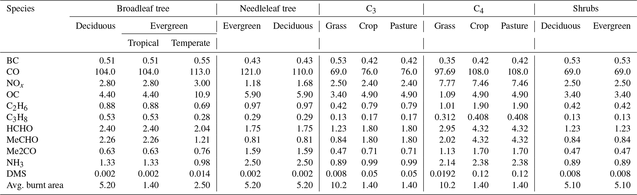
The emitted carbon per PFT, ECPFT (), in Eq. (2) is calculated based on the burnt area and combustion completeness, accounting for the wetness of fuel. INFERNO also represents emissions for trace gases: carbon dioxide (CO2), carbon monoxide (CO), methane (CH4), nitrogen oxide (NOx), sulfur dioxide (SO2), ethane (C2H6), propane (C3H8), formaldehyde (HCHO), Acetaldehyde (MeCHO), acetone (Me2CO), ammonia (NH3), dimethyl sulfide (DMS); and aerosols: OC and BC. These emissions are estimated based on INFERNO's emitted carbon estimate (Eq. 2) by using the emission factors based on the work by Andreae (2019) as shown in Table 1.
CCmin and CCmax are the minimum and maximum combustion completeness for both leaves (CCmin=0.8 and CCmax=0.9) and stems (CCmin=0.2 and CCmax=0.4), Ci is the carbon stored in each PFT leaves or stem and θ the unfrozen soil moisture as a fraction of saturation.
INFERNO fire ignitions are split into natural ignitions (IN) (ignition m2 s−1) from cloud-to-ground lightning (externally provided to INFERNO) and anthropogenic ignitions (IA) (ignition m2 s−1) which are dependent on population density (PD) (people m−2) as described in Eq. (3). Moreover, it is assumed that humans are also responsible for suppressing fires which is accounted for through a suppression function dependent on human population density given by Eq. (4). Originally, Eqs. (3) and (4) were developed to include only information on population density. We now include a human development index (HDI) term (1−HDI) in these equations that represents socio-economic factors impacting fire ignition and suppression. HDI is calculated based on three indicators designed to capture the income, health and education dimensions of human development. For areas where there is more effort in human development improvements, it is assumed that fire ignition is decreased, and fire suppression is increased.
HDI data were obtained from the gridded global datasets for gross domestic product and human development index (Kummu et al., 2018). The anthropogenic ignitions (IA) (ignition m2 s−1) is represented by Eq. (3), the fraction of fires not suppressed by humans (fNS) by Eq. (4) and the total ignitions (IT) are represented by Eq. (5).
where is a function that represents the varying anthropogenic influence on ignitions in rural versus urban environments, the parameter α=0.03 represents the number of potential ignition sources per person per month per km2, IN represents the natural ignitions due to lightning and HDI the human development index.
Furthermore, it should be highlighted that in this configuration of INFERNO, there are no interactions between fire and vegetation, and it does not include a peat-burning capability.
2.2 UK Earth System Model (UKESM1)
This study uses the atmospheric and land components of UKESM1 (Sellar et al., 2019, 2020) following the protocol set by the Atmospheric Model Intercomparison Project (AMIP, Eyring et al., 2016). The model resolution used in this configuration is N96L85. This is equivalent to a horizontal resolution of 135 km in the midlatitudes and 85 terrain-following vertical levels ranging up to an altitude of 85 km above sea level. The science configuration of the atmosphere component is based on the Global Atmosphere 7.1 (GA7.1) and the Global Land 7.0 (GL7.0) as described by Walters et al. (2019) used in the configuration of the Hadley Centre Global Environment Model version 3 (HadGEM3; Hewitt et al., 2011) coupled to the terrestrial carbon/nitrogen cycles (Sellar et al., 2019) and interactive stratosphere–troposphere chemistry (Archibald et al., 2020) from the UK Chemistry and Aerosol (UKCA; Morgenstern et al., 2009; O'Connor et al., 2014) model. The framework also includes the UKCA prognostic aerosol GLOMAP-mode scheme (Carslaw et al., 2010; Mulcahy et al., 2019), where secondary aerosol formation is determined by interactive oxidants from the UKCA stratosphere–troposphere chemistry scheme (Archibald et al., 2020).
As per the AMIP protocol, sea surface temperature and sea ice are taken from the unmodified dataset of Durack and Taylor (2017) and horizontally interpolated to the model resolution. In this model setup, the dynamic vegetation model (TRIFFID, Cox, 2001) is deactivated and replaced by prescribed vegetation properties from a coupled historical simulation with the same base model, as shown in Fig. 1, preserving consistency in the forcing due to land use change between the UKESM1 coupled and AMIP experiments. In a similar fashion, seawater concentrations of dimethyl sulfide (DMS) and chlorophyll-a monthly climatologies are taken from the coupled historical experiment and are used by the atmosphere model top calculates fluxes of DMS and primary marine organic aerosol (Mulcahy et al., 2019).
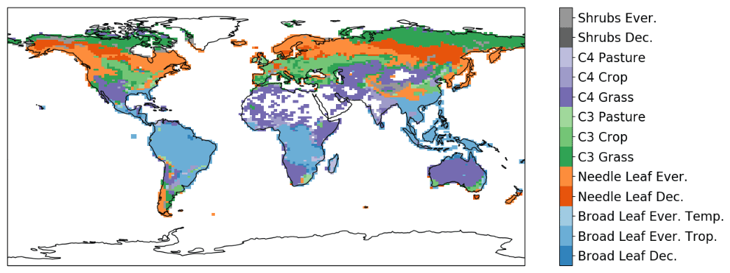
Figure 1Dominant vegetation PFT per grid box for as prescribed in UKESM1-AMIP configuration.
External forcing datasets for biomass burning aerosol and trace gas emissions follow those stipulated under the coordination of the CMIP6 protocol (Van Marle et al., 2017). These are a combination of satellite observations from 1997 with various proxies and modelling results from six fire models which have participated in the Fire Model Intercomparison Project (Rabin et al., 2017) aimed at providing a dataset of biomass burning emissions for use in CMIP6. UKESM1 uses emissions of primary carbonaceous aerosol – black carbon (BC) and organic carbon (OC) – as well as DMS, which acts as a precursor to sulfate aerosol. In terms of gas-phase biomass burning emissions, UKESM1 uses lumped emissions of ethene (C2H4) and ethane (C2H6) as C2H6, and emissions of propane (C3H8), formaldehyde (HCHO), acetone (CH3)2CO), acetaldehyde (CH3CHO), carbon monoxide (CO) and nitric oxide (NO). Aerosol emissions of BC and OC from biomass burning are spread evenly in the vertical over the first 20 model levels – corresponding to the lowest 3 km – and are treated with a geometric mean diameter of 150 nm, while all other biomass burning trace gas species are injected into the model's lowest layer and mixed simultaneously by the boundary layer mixing scheme. A biomass burning emissions scaling factor of 2 is applied to biomass burning aerosols, following the evaluation work of Johnson et al. (2016), which improves the agreement between observed and simulated aerosol optical depth (AOD) across the three evaluated wave lengths (440, 550, 700 nm) when compared to observations. This AOD bias is also evident in the comparison of previously published top-down and bottom-up estimates and using a scaling factor correction is a practice widely used in the modelling community due to current model deficiencies (Kaiser et al., 2012).
Annual anthropogenic emissions of reactive gases are prescribed to the model and are taken from the Community Emissions Data System (CEDS, Hoesly et al., 2018) as prepared for use in CMIP6. Both biomass burning and anthropogenic emissions datasets are regridded from their native resolution to N96L85 while conserving global annual totals and seasonal cycles.
A set of natural emissions of other species which are not simulated by UKESM1 is prescribed through precomputed fluxes. This includes emissions of oceanic emissions of CO, C2H6 (including C2H4 lumping) and C3H8 (including propene (C3H6) lumping) from POET (Granier et al., 2005) and correspond to the annual cycle inventory for the year 1990 (12 monthly fluxes). Biogenic emissions of CO, HCHO, MeOH, C3H6 and C3H8, as well as CH3CHO and MeCHO are taken from the MACCity-MEGAN emissions inventory (Sindelarova et al., 2014) and are provided to the model based on the 2001–2010 monthly mean climatology. Soil emissions of NOx are distributed according to Yienger and Levy (1995) and scaled to give a global annual total of 12.0 Tg NO yr−1, perpetually applied to all years.
Further details on the UKESM1 model setup can be found in Sellar et al. (2020) and further details (e.g. lightning NOx emissions, lower boundary conditions, interactive BVOC emissions) and an evaluation of the performance of the UKCA chemistry and aerosol schemes in UKESM1 are available in Archibald et al. (2020) and Mulcahy et al. (2019).
2.3 Fire–composition–atmosphere coupling
JULES is the land surface model used in UKESM1, and a coupling interface is in place for the exchange of variables and drivers between the atmosphere and land components. For this work, the interface was extended to allow the coupling of the required atmospheric variables from the atmospheric model to INFERNO through JULES. The atmospheric model provides to INFERNO the surface pressure, 1.5 m temperature, 1.5 m specific humidity and precipitation at every model time step. Temporal variations of lightning can have a large impact on the simulation of burned area (Felsberg et al., 2018). With this in mind, and to maintain consistency between fire lighting ignitions, the state of the atmosphere and atmospheric composition, the cloud-to-ground lightning simulated by UKESM1 is passed down to INFERNO. The lighting parametrization used follows the work of Price and Rind (1994), which makes use of parameterized lightning flash frequency of min−1 over land and min−1 over ocean (where H is the cloud depth in kilometres), along with a cloud–cloud and cloud–ground flash ratio based on the grid-cell latitude. The cloud depth is determined using the convective cloud base and top levels diagnostics from the convection scheme.
Conversely, in order to allow for fire–climate interactions through atmospheric chemistry and aerosols, the coupling framework was extended to pass INFERNO-derived emissions to the UKCA chemistry and aerosol model of CO, NOx, C2H6, C3H8, HCHO, MeCHO, Me2CO, NH3, DMS, OC and BC at every model time step. As described by Archibald et al. (2020), in UKESM1, biomass burning emissions of C2H6 and C3H8 include emissions of C2H4 and C3H6, respectively. In this interactive fire emissions framework, we do not consider this emission aggregation, and considering the small contribution of biomass burning to these species (15.7 % for C2H6 and 13.6 % for C3H8), we do not consider this to have a large impact on the modelled results.
Aerosol emissions are distributed vertically following an exponential increasing function (emission increasing with height) from the first model level to a fixed top of plume height defined as the 20th model level (∼3 km). This approach is a simplification based on the work of Rémy et al. (2017). This new fire–atmosphere interaction replaces the prescribed transient monthly varying biomass burning emissions in UKESM1. As a result, through atmospheric chemistry and aerosols, the interactive fire emissions can affect radiation and clouds, thereby affecting weather/climate and the meteorological drives of fires themselves.
The model experiments were run for the period 1974 to 2014 and the initial 5 years (1974–1979) were considered as simulation spin-up and discard from the analysis.
For the sake of brevity, from here onwards, this fire–composition–atmosphere coupled configuration based on UKESM1 is referred to as UKESM1+INFERNO.
2.4 Burnt area and emissions evaluation
Burnt area data from the Global Fire Emissions Database version 4 (GFED4s) (Giglio et al., 2013) were used to assess the performance of the UKESM1+INFERNO in modelling fires. This dataset is provided as a gridded product at a 0.25∘ resolution and is derived from a multi-sensor satellite dataset, including satellite dataset based on active fire detection, including small fires, based on statistical modelling, as detailed in Randerson et al. (2012).
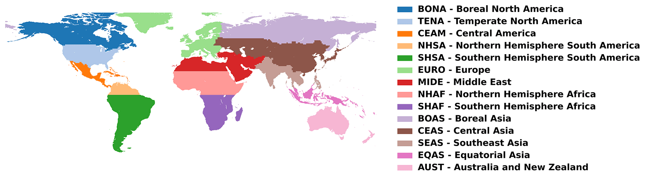
Figure 2Basis regions, as defined in the GFED4s dataset (Giglio et al., 2013).
The basis regions as defined in the GFED4s dataset (Fig. 2) were applied to the modelled data as required in order to perform a regional assessment of the INFERNO results. From here after, these regions will be named according to the acronyms defined in Fig. 2.
To evaluate the fire emissions from INFERNO within the global ESM, the data from Global Fire Assimilation System (GFAS) were used. GFAS calculates biomass burning emissions by assimilating satellite observations of fire radiative power (FRP) from the Moderate Resolution Imaging Spectroradiometer (MODIS) Aqua and Terra satellites (Kaiser et al., 2012). Combustion rates in GFAS are calculated with land-cover-specific conversion factors which have been derived from a linear regression analysis between the FRP of GFAS and the dry matter combustion rate of GFED (Heil et al., 2010). Emissions for 40 gas-phase and aerosol trace species are then calculated by applying emission factors based on the works of Andreae and Merlet (2001), Christian et al. (2003) and Akagi et al. (2011). Daily emissions are available on a global grid from 2003 to the present day.
2.5 AOD and extinction coefficient evaluation
Both ground-based measurements and satellite retrievals of AOD are used to evaluate the model performance. Ground-based measurements from the Aerosol Robotic Network (AERONET) provides quality assured measurements of aerosol optical properties across the globe (Holben et al., 1998, 2001). For this study, the monthly AOD at 440 nm is used from the version 2 level 2.0 product for stations that have at least a 5-year overlapping period with the model simulations. AOD evaluation is complemented with data from satellite retrievals. The MODIS aerosol product provides daily observations of the AOD with a global coverage. We used the collection of the level 3 V6 MODIS monthly data of AOD at 550 nm for the period from January 2003 to December 2012, which is produced from daily means blending the Dark Target and Deep Blue algorithms (Hsu et al., 2004; Sayer et al., 2014) and provided as gridded data at a 1∘ spatial resolution.
To evaluate the vertical profile of aerosol, the Cloud–Aerosol Lidar and Infrared Pathfinder Satellite Observations (CALIPSO) lidar level 3 aerosol extinction coefficient profiles product at 532 nm were used. This product reports monthly mean profiles of aerosol optical properties and is quality screened prior to averaging on a uniform spatial grid with a meridional and zonal resolution of 2 and 5∘ respectively and a vertical resolution of 60 m. For comparison with model results, the focus is on clear sky averages (Tackett et al., 2018).
2.6 Carbon monoxide
Evaluation of the gas-phase biomass burning emissions is focused on carbon monoxide (CO), the most abundant chemically active pollutant emitted by fires (van der Werf et al., 2010). For this, model results are evaluated against observations from the Tropospheric Emission Spectrometer (TES-AURA), which have been used before to evaluate CO in previous versions of UKCA (O'Connor et al., 2014; Voulgarakis et al., 2011). We have used TES-AURA-Lite version 007 data (Beer et al., 2001; Bowman et al., 2006) covering the 5-year period between 2007–2012 where there were fewer data gaps. To compare model results with TES-AURA observations, the hourly CO model output has been interpolated onto the 14 TES-AURA-Lite pressure levels, as well as satellite swath location. Furthermore, the TES-AURA sampling and averaging kernels and a priori profiles were also applied to the model data. Both TES-AURA and modelled processed data are then monthly averaged into a resolution grid. Only the vertical region where TES-AURA is more sensitive to CO was used – average over the vertical column between 700 and 300 hPa.
In this section, the results of the implementation of the fire–composition–atmosphere coupling in UKESM1+INFERNO are analysed. When comparing datasets (model or observed) with different grid resolutions, the higher resolution dataset is regridded to the lowest resolution grid using a first-order conservative area-weighted regridding method. Statistical significance of the differences presented here were examined using a Student's t test (Wilks, 2011) with a 95 % confidence level.
3.1 Burnt area
Figure 3 shows the annual mean burnt area fraction (1997–2010) for (a) UKESM1+INFERNO and (b) GFEDv4. The overall geographical pattern of the annual average burnt area fraction is well reproduced by the model with a global pattern correlation of 55.3 % when compared with GFEDv4. The model represents the observed pattern in the major fire regions: South America, Africa and Eurasia. On the other hand, the model underestimates the northern Australia fires and boreal regions. Although the burnt area fraction over Africa is well represented, there is a large (50 %) underestimation of the fires over Africa in the northern African region (NHAF). This underestimation can be attributed to the Saharan bare soil extending too far south, causing a lack of grassland in the Sahel region, which is a result of precipitation deficits associated with errors in the position and intensity of monsoon systems (Sellar et al., 2019; Williams et al., 2018). In addition, there is an overestimation of tree fraction in savanna biomes, such as the southern African region (SHAF) and the southern edge of the Amazon rain forest region (SHSA). The differences in the specified scaled average burnt areas for these biomes – smaller for trees than grasses – cause an underestimation of fire size in these regions. This overestimation of the tree fraction is attributed to the lack of fire disturbance in the fully coupled UKESM1 configuration, the inclusion of which could potentially improve vegetation structure in these regions (Burton et al., 2019).
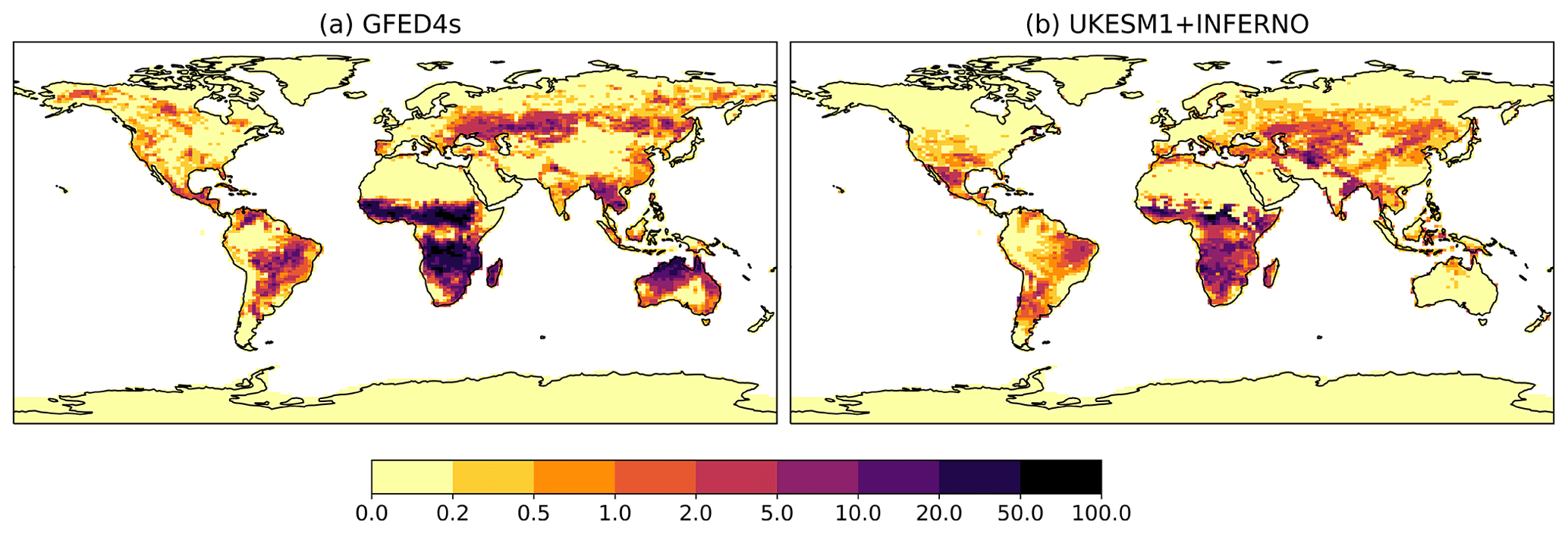
Figure 3Burnt area fraction (%) mean annual average (1997–2010) for (a) GFED4s and (b) UKESM1+INFERNO.
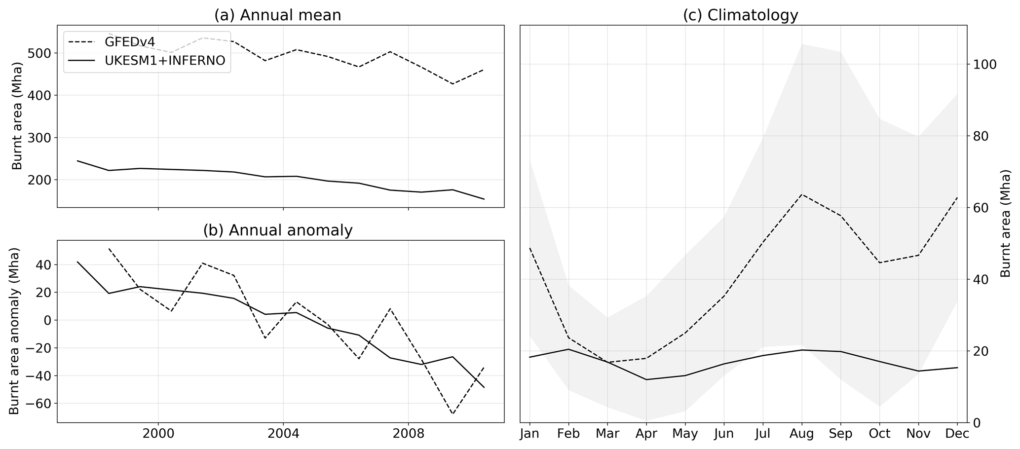
Figure 4Burnt area annual mean time series (a, b) anomaly relative to climatology (Mha) and (c) burnt area fraction climatology (%) for UKESM1+INFERNO (solid line) and GFEDv4 (dashed line) with the shaded area representing the standard error around the GFEDv4 data.
These biases found for the different regions have an impact on the modelled global fire behaviour. Although there is a global underestimation of the annual average burnt area of approximately 250 Mha (Fig. 4a), the model is able to capture the negative trend found in the observations (Fig. 4b). In terms of seasonality, the model produces a bimodal pattern in the fire activity, as observed in GFEDv4, which peaks around both the austral and boreal late summer season.
Although there is a global underestimation contributing to the interannual variability of burnt area, it is important to stress that the biases found in NHAF and SHAF contribute to most of the biases found in the global burnt area climatology. A November-to-January difference of 45 Mha for the NHAF region combined with a July-to-September difference of 30 Mha results in an absolute bias of greater than 300 %, as can be seen in Fig. 5.
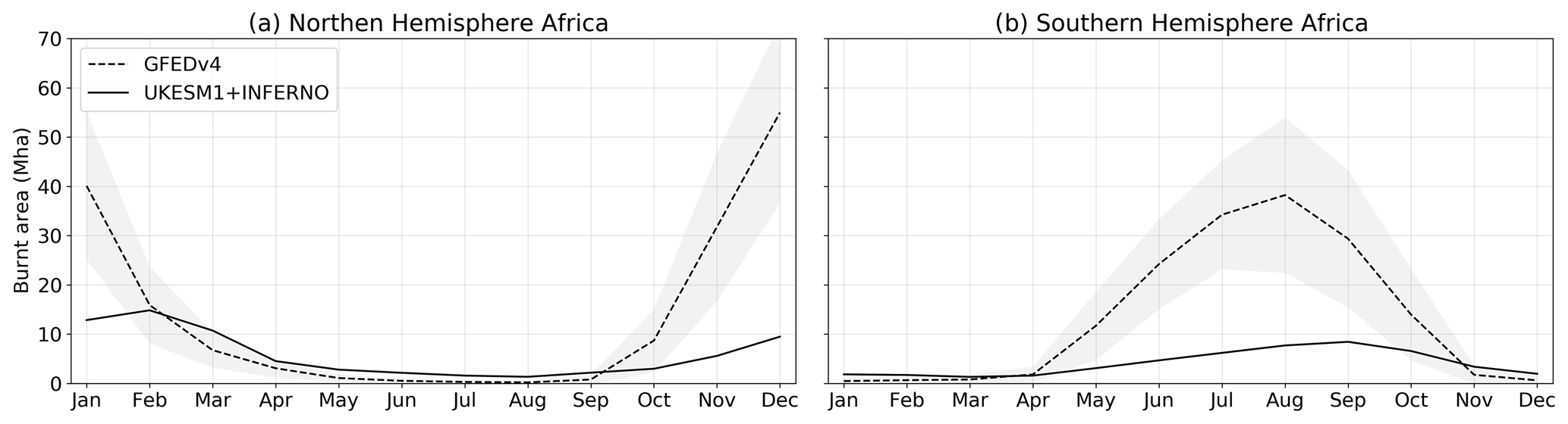
Figure 5Burnt area fraction climatology (%) for UKESM1+INFERNO (solid line) and GFEDv4 (dashed line) with the shaded area representing the standard error around the GFEDv4 data for NHAF (a) and SHAF (b).
3.2 Biomass burning emissions
In order to develop a full fire–composition–climate ES model, it is paramount to evaluate the ability of the INFERNO – UKESM1 coupling with regards to providing realistic emissions of chemistry and aerosol species. Currently this coupling framework provides trace gases emissions of CO, NOx, C2H6, C3H8, HCHO, DMS, NH3 and DMS, as well as aerosol emissions of OC and BC. These emissions are estimated based on INFERNO emitted carbon by using PFT-specific emission factors. For this reason, the different species present similar broad characteristics. With this in mind and considering the observed datasets available and used to assess the model performance, we will focus on the analysis of CO, OC and BC.
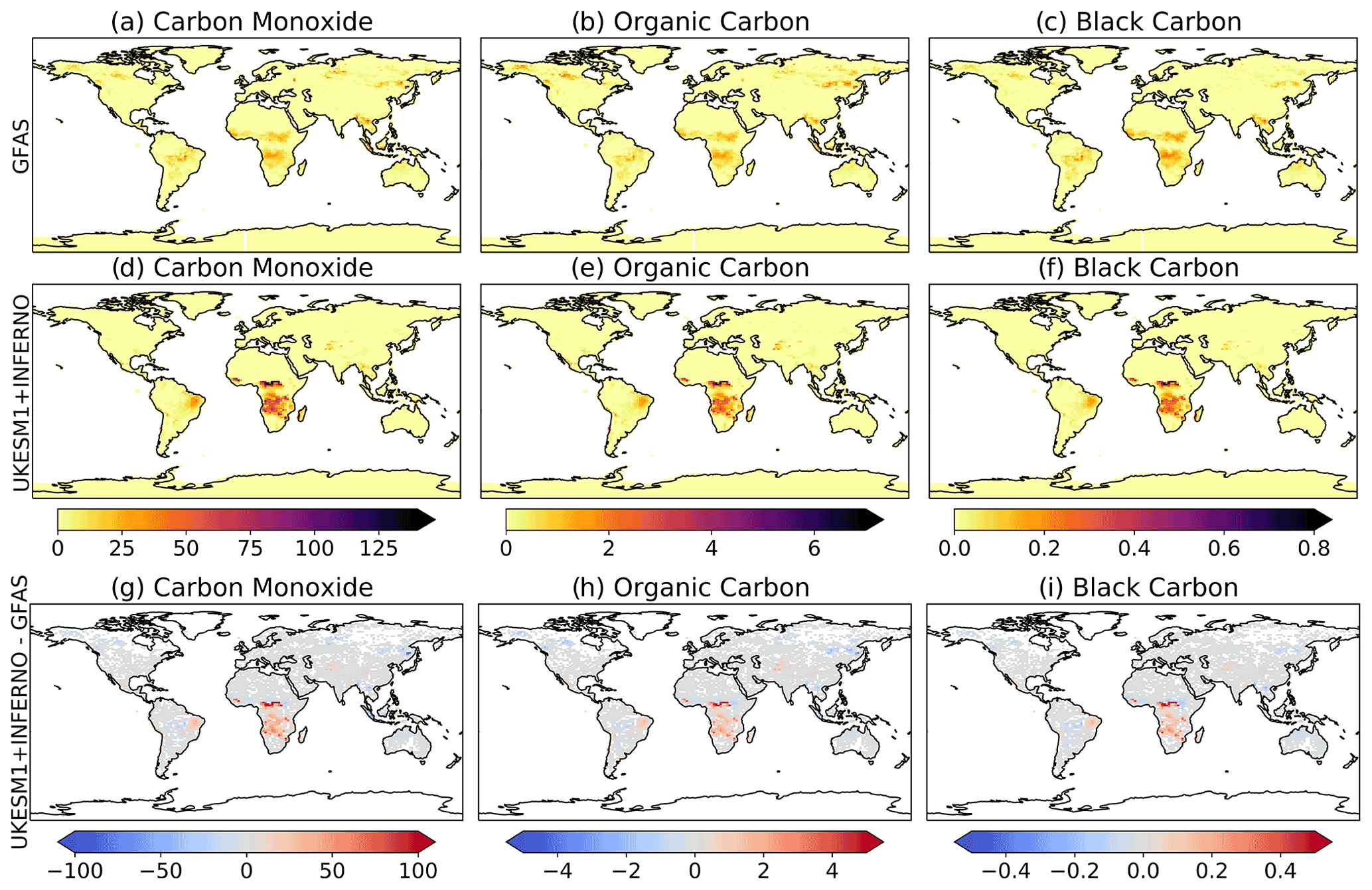
Figure 6Biomass burning emissions mean annual average (2003–2011) for CO (g m−2) in (a) GFAS, (d) UKESM1+INFERNO and (g) difference between UKESM1+INFERNO and GFEDv4; OC (g m−2) in (b) GFAS, (e) UKESM1+INFERNO and (h) difference between UKESM1+INFERNO and GFEDv4 and BC (g m−2) in (c) GFAS, (f) UKESM1+INFERNO and (i) difference between UKESM1+INFERNO and GFAS. Differences are only shown for statistically significant points with a 95 % confidence level.
As seen for the burnt area results, the overall global pattern for annual average biomass burning emissions is, in general, well reproduced by the model (Fig. 6). The main regions of biomass burning emissions, Africa and South America, are captured in the global spatial pattern. However, there is a large overestimation of the biomass burning emissions, despite underestimation of area burned, in the southern edge of NHAF, SHAF as well as the eastern side of SHSA for all the species (difference>300 %). Furthermore, in the SHAF region, the emissions extend further south into the midlatitudes. These overestimations can be attributed to the overestimation of the tree fraction in these regions leading to a greater content of carbon available for combustion. On the other hand, the model underestimates the emissions for the boreal regions (emissions close to zero in the model). These biases result in smaller values of global pattern correlation for biomass burning emitted species of 36.7 % for CO, 38.4 % for OC and 53.2 % for BC when compared with GFAS. UKESM1+INFERNO shows a good climatological performance (no large bias; Fig. 6) for equatorial Asia (EQAS). However, it fails to reproduce specific large fire events (that are infrequent) associated with peatland fires that represent a substantial amount of the global biomass burning emissions (not shown). We do not expect the model to be able to capture such emission events, as the current land surface model does not include a peatland land class, and therefore we do not include a peat-burning capability. However, it should be noted that although we have a negative bias relative to the observations, the observations themselves may be biased due to the lacking efficiency in detecting low-temperature smouldering peat fires in MODIS products used by GFED4s and GFAS.
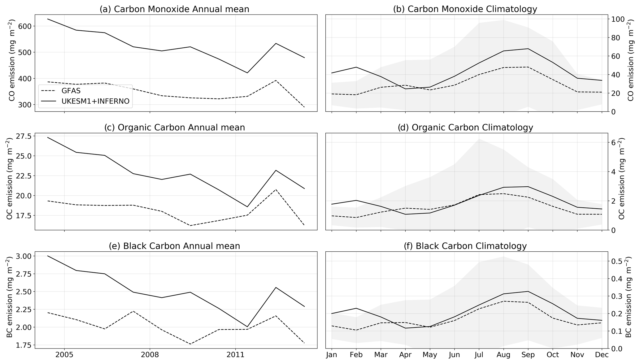
Figure 7Annual mean time series and seasonal cycle climatology of biomass burning emissions (mg m−2) of CO (a, b), OC (c, d) and BC (e, f) for UKESM1+INFERNO (solid line) and GFAS (dashed line). The shaded area represents the standard error in the GFAS data.
The biomass burning emission (kg m−2) annual mean time series and climatology (Fig. 7) show that there are large biases in the annual mean time series for all the emissions. When compared to GFAS, CO shows a root mean squared error (RMSE) of 349.53 mg m−2 and a correlation of 74.79 %, whereas OC shows a RMSE of 10.08 mg m−2 and BC a RMSE of 1.08 mg m−2. Both simulated OC and BC show non-significant correlation (when tested with a 95 % confidence level) of 56.06 % and 49.41 %, respectively. Despite this, there is a good agreement to their observations with regards to the interannual variability and climatology, with the model capturing the negative emission trends in the 1997–2010 period and being able to reproduce the observed seasonal cycle – higher emissions of CO, OC and BC during the period from June to October (in Fig. 7b, d and f, respectively). Despite the non-significant correlation between the interannual time series, there is good qualitative agreement for both interannual and seasonal variability. This is partly due to the compensation of regional biases and partly due to the burnt area bias. The low correlations obtained for OC and BC interannual time series are mainly due to the overestimation of the negative trend by the model.
3.2.1 Sensitivity to land surface
In order to better understand the impact of the overestimation of tree fraction in savanna biomes, sensitivity experiments were performed where the dominant tree PFT is replaced with an equal quantity of the dominant grass PFT. We focus on a region over SHAF, characterized by a savanna biome, but where in UKESM1 is dominated by broadleaf evergreen tropical trees (∼70 % of total PFT fraction) – latitudes between 3.0 and 29.0∘ S and longitudes between 7.0 and 42.0∘ E.
Two sensitivity experiments were performed where, for this specific region, the broadleaf evergreen tropical trees are replaced by C4 grasses and run for the period 1980–1985:
-
T2G10 – 10 % of trees are changed to grass.
-
T2G50 – 50 % of trees are changed to grass (this experiment has the closest representation of the observed land surface).
In the SHAF region, which includes the area where the PFTs were changed; there are 12.17 % and 79.83 % increases of the burnt area for 10 % and 50 % changes in the tree cover into grasses, respectively (T2G10 and T2G50, Table 2). Thus, regionally, the modelled burnt area is hypersensitive to a change of the underlying vegetation (the change in burnt area is greater than the change in vegetation cover fraction). In contrast, for the case of biomass burning emissions, there is much less sensitivity to a change in the vegetation cover. In this case, for a 10 % change of the dominant tree to the dominant grass PFT (T2G10), there were no statistically significant changes to emissions. However, a statistically significant decrease of ∼14 %–25 % is found for T2G50, showing that, although biomass burning emissions are hyposensitive to a change of the underlying vegetation, when there is a larger change to the underlying vegetation, this can result in significant changes.
Table 2Total annual average values and relative change (%) compared to UKESM1+INFERNO (period between 1980–1985) of burnt area (Mha), carbon monoxide (g m−2), organic carbon (g m−2) and for black carbon (g m−2) for UKESM1+INFERNO and the different sensitivity experiments, T2G10 and T2G50 – global and SHAF regions. Values in bold show that the difference between a given experiment and UKESM1+INFERNO is statistically significant with a 95 % confidence level.
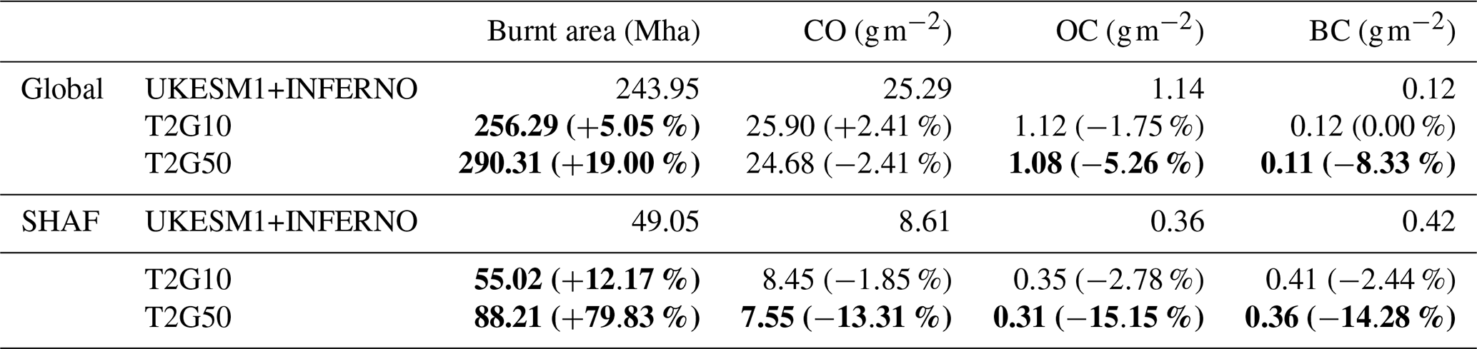
This sensitivity to the underlying vegetation can also have a significant impact at the global scale for both burnt area (statistically significant increase of 5.05 % and 19.00 % for T2G10 and T2G50, respectively) and biomass burning emissions (significant decreases of 5.26 % and 8.33 % for OC and BC in T2G50, respectively). The change applied to the vegetation causes significant changes in both burnt area and biomass burning emissions not only locally but also for regions away from the area where the vegetation was changed, through changes in atmospheric dynamics at a global scale (Fig. 8). However, further work is required to assert if these changes are mainly associated with the change to the land cover or the fire–atmosphere–composition feedbacks. This strongly indicates that a realistic representation of the vegetation distribution could significantly improve the model performance when compared to observations.
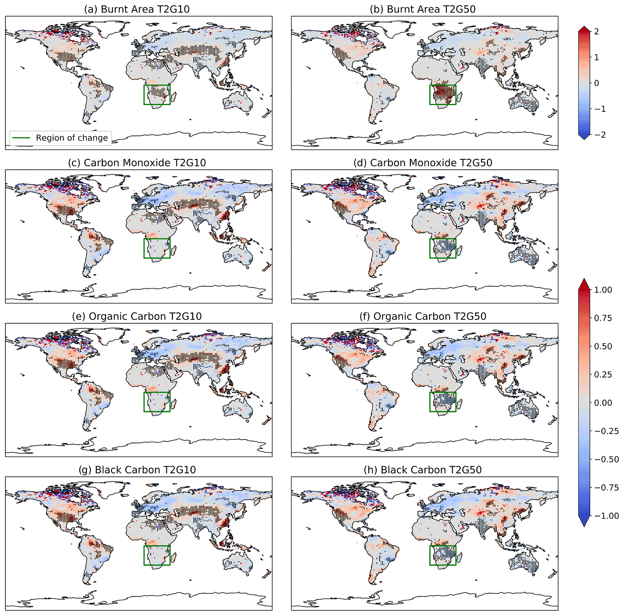
Figure 8Total annual average fractional of change (period between 1980–1985) of burnt area (Mha), carbon monoxide, organic carbon and for black carbon for the UKESM1+INFERNO and the different sensitivity experiments, T2G10 and T2G50. Stippling is shown for points where the difference between a given experiment and UKESM1+INFERNO is statistically significant with a 95 % confidence level. The green rectangle indicates the area where the prescribed vegetation was changed.
3.3 Carbon monoxide atmospheric column
When analysing the CO mean column mixing ratio averaged between 700 and 300 hPa (Fig. 9), it is possible to see that the atmospheric column of CO is dominated by the hot spots of biomass burning over South America and Africa and anthropogenic emissions in the Northern Hemisphere, with a strong north–south hemispheric gradient due to the short life time of CO – approximately 30 d – compared to the timescale of interhemispheric mixing.

Figure 9Column volume mixing ratio carbon monoxide (ppm) averaged between 700 and 300 hPa over the period 2007–2012 for (a) TES-AURA satellite retrievals, (b) UKESM1+INFERNO, (c) difference between UKESM1 and TES-AURA, and (d) difference between UKESM1+INFERNO and TES-AURA.
When comparing the model results to TES-AURA, it can be seen that there is an underestimation of the column CO in the northern hemisphere. This underestimation happens both in UKESM1 (Fig. 9c) and UKESM1+INFERNO (Fig. 9d). As documented by Archibald et al. (2020), these negative biases can be attributed to insufficient secondary production of CO from non-methane volatile organic compound oxidation and strong loss through hydroxyl radicals (OH) in the Northern Hemisphere. Archibald et al. (2020) also showed that, for UKESM1, there is a positive bias associated with regions where CO emissions are dominated by agricultural (eastern Central Asia region) and forest fires in central Africa (NHAF and SHAF) and the northwestern part of South America (NHSA). In UKESM1+INFERNO, the bias found in the CO column is similar to the ones found in UKESM1. However, the overestimation of biomass burning emissions of CO on the southern edge of NHAF and SHAF, previously described in Sect. 3.1, is reflected in a higher column CO positive bias in UKESM1+INFERNO when compared with TES-AURA for these regions. For South America (NHSA and SHSA regions), UKESM1+INFERNO shows an improvement in the western and central parts of NHSA but an increase of the negative bias in the southern and eastern parts of SHSA.
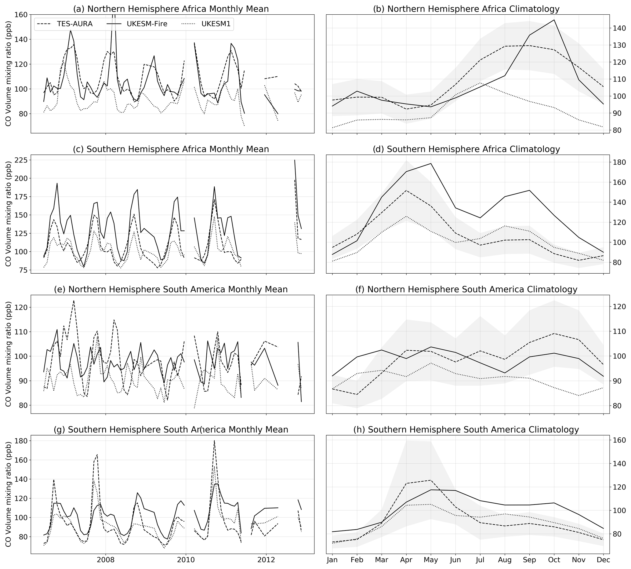
Figure 10Column volume mixing ratio of carbon monoxide (ppm) averaged between 700 and 300 hPa for the period 2007–2012 (a) monthly mean time series and (b) monthly mean climatology for the NHAF region, (c) monthly mean time series and (d) monthly mean climatology for the SHAF region, (e) monthly mean time series and (f) climatology for the NHSA region, and (g) monthly mean time series and (h) monthly mean climatology for the SHSA region – UKESM1+INFERNO (solid line), UKESM1 (dotted line) and TES-AURA (dashed line).
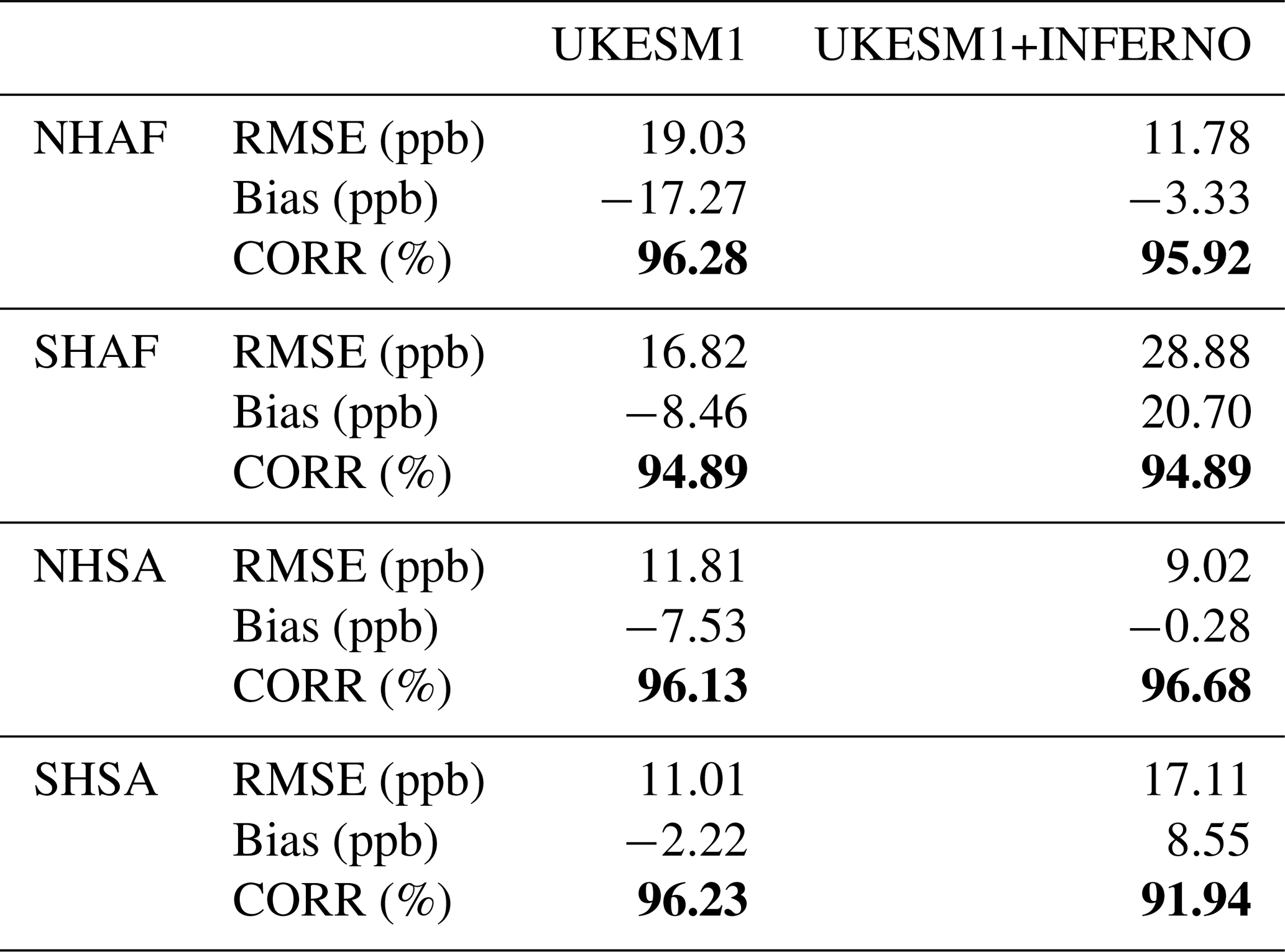
A comparison of the monthly mean time series and monthly mean climatology between TES-AURA, UKESM1 and UKESM1+INFERNO for the main fire regions – NHAF, SHAF, NHSA and SHSA – is shown in Fig. 10 and provides information on interannual variability and the climatology of the regions that dominate the differences in the CO atmospheric column between UKESM1 and UKESM1+INFERNO. In most of these regions, the UKESM1+INFERNO configuration tends to provide an improvement on the modelled volume mixing ratio of CO, for NHAF (Fig. 10a and b), reducing the negative bias and RMSE of UKESM1 from −17.27 to −3.33 and 19.03 to 11.78 ppb, respectively. However, both configurations show a similar correlation of 96.28 in UKESM1 % and 95.92 % in UKESM1+INFERNO. These improvements are mostly associated with the decreases of the CO atmospheric column between May and August for UKESM1+INFERNO and the improvement of the variability over this region. As can be seen in Fig. 10c, SHAF is the region with the largest changes when comparing UKESM1 and UKESM1+INFERNO. When compared to TES-AURA, there is a significant worsening of the bias caused by the higher emissions over this region – from −8.46 to 20.70 ppb for UKESM1 and UKESM1+INFERNO, respectively. In addition, the RMSE is also increased from 19.03 ppb in UKESM1 to 28.88 ppb in UKESM1+INFERNO. Despite this, both configurations show similar high correlations with TES-AURA (94.89 % and 94.89 % for UKESM1 and UKESM1+INFERNO, respectively). These results show that, despite the large bias caused by the vegetation errors for this region, the UKESM1+INFERNO configuration captures the observed variability of CO, representing the two peaks in CO that occur in April and August. This can be seen both in monthly mean time series, as well as in the climatology for SHAF (Fig. 10d).
With regards to South America, there is an improvement in the NHSA region (Fig. 10e and f), with UKESM1+INFERNO presenting lower values of RMSE and bias than UKESM1 when compared to TES-AURA – RMSE reduction from 11.81 to 9.02 ppb and bias from −7.53 to −0.28 ppb – and the correlation presenting similar values 96.13 % for UKESM1 and 96.68 % for UKESM1+INFERNO. Even so, as depicted in Fig. 10f, for this region, UKESM1+INFERNO produces a more pronounced bimodal seasonality of CO atmospheric column peaking in late April and October, consistent with observations, but underestimates the magnitude especially for October, failing to represent years when concentrations are kept high during the summer months. It is worth noting that these results may be affected by the advection of CO from the SHAF region. In the SHSA region (Fig. 10g and h), UKESM1+INFERNO does not perform as well as UKESM1. Despite a good correlation with TES-AURA (91.94 %), the peak in CO volume mixing ratio tends to extend for longer periods of time throughout the year (from May to November) which results in a larger positive bias (8.55 ppb in UKESM1+INFERNO and −2.22 ppb in UKESM1). The results of the statistical comparison of the monthly mean time series, between the UKESM1 and UKESM1+INFERNO configurations with TES-AURA, are summarized in Table 3.
Table 3Statistical comparison – root mean squared error (RMSE), bias and Pearson correlation coefficient (CORR) – of the monthly average time series between UKESM1 and UKESM1+INFERNO with TES-AURA for the period 2007–2012. Values in bold show that the correlation between a given experiment and TES-AURA is statistically significant with a 95 % confidence level.
3.4 Aerosols
Aerosols have a large effect on the Earth's radiative budget and climate; they can scatter and absorb radiation, as well as change cloud proprieties leading to changes in cloud cover and precipitation (Ward et al., 2012). As shown by Liousse et al. (1996), biomass burning is the primary source of natural carbonaceous aerosols in the ES (OC and BC), making them a major influence in controlling the ES variability in regions where fire activity is dominant. To evaluate the model's ability to reproduce the observed distribution and variability of aerosols, we compare the model to aerosol products from three instruments: MODIS and AERONET for AOD and CALIPSO for the vertical profile of the aerosol extinction coefficient. The focus is on the global distribution, seasonality and interannual variability of the major fire regions – NHAF, SHAF, NHSA and SHSA.
Mulcahy et al. (2019) provides a comprehensive model evaluation of aerosols in UKESM1 using prescribed fire emissions. In their study, the authors showed that the model performs well when compared to observations, capturing the global spatial distributions of AOD and cloud droplet number concentrations. The authors also report regional biases, including an overestimation of droplet number concentrations in the marine stratocumulus cloud regimes and an underestimation of aerosol optical depth in dust-dominated regions (Fig. 11c).

Figure 11Aerosol optical depth multi-year average annual mean at 550 nm (2003–2012) for (a) MODIS, (b) UKESM1+INFERNO, (c) difference between UKESM1 and MODIS, and (d) difference between UKESM1+INFERNO and MODIS. Differences are only shown for statistically significant points with a 95 % confidence level.
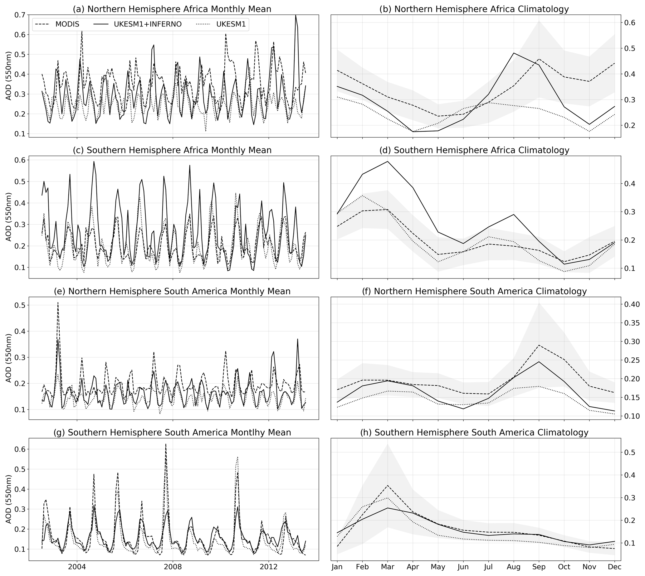
Figure 12Aerosol optical depth at 550 nm for the period 2003–2012 (a) monthly mean time series and (b) climatology of monthly means for the NHAF region, (c) monthly mean time series and (d) climatology of monthly means for the SHAF region, (e) monthly mean time series and (f) climatology of monthly means for the NHSA region, and (g) monthly mean time series and (h) climatology of monthly means for the SHSA region – UKESM1+INFERNO (solid line), UKESM1 (dotted line) and MODIS (dashed line).
This section focuses on the evaluation of UKESM1+INFERNO. When compared to MODIS, the annual mean of aerosol optical depth simulated by UKESM1+INFERNO (Fig. 11) has a realistic global spatial pattern. The global RMSE is 0.07, the bias is −0.07, and the global pattern correlation between the two model simulations is 79.7 %. Focusing on the main fire regions, the UKESM1+INFERNO tends to overestimate the AOD over Africa (both NHAF and SHAF), as well as SHSA and underestimate it in NHSA. Looking at the monthly mean time series and climatology of monthly means for AOD at 550 nm (Fig. 12), overall for the NHAF region (Fig. 12a and b), the UKESM1 and UKESM1+INFERNO results are dominated by a negative bias when compared to MODIS. This is found to be associated with the dust aerosol bias, as described in Mulcahy et al. (2019). Nonetheless, the southern edge of this region is dominated by fire emissions and both model configurations tend to overestimate the AOD, with an increase of the bias for UKESM1+INFERNO. Comparing the time series for this region (Fig. 12a), the higher biomass burning emissions of OC and BC in UKESM1+INFERNO compensates for the lack of dust emissions which results in a smaller bias and larger RMSE for UKESM1+INFERNO when compared to UKESM1 (bias of −0.06 from −0.10 and RMSE of 0.14 from 0.12). The pattern correlation of mean monthly values in UKESM1+INFERNO is also improved, when we compare to UKESM1 (from 21.02 % to 37.2 %). On the other hand, the AOD in the SHAF region (Fig. 12c and d) is dominated by biomass burning emissions and, as seen for CO, UKESM1+INFERNO tends to overestimate the biomass burning emissions due to the overestimation of tree fraction in this region. This leads to more OC and BC emissions. When comparing the time series between the two model configurations and MODIS (Fig. 12c), there is a change of signal, as well as an increase in the bias (from −0.003 in UKESM1 to 0.056 in UKESM1+INFERNO) and RMSE (from 0.05 for UKESM1 to 0.11 UKESM1+INFERNO). In terms of spatial correlation (Fig. 11), both models are highly correlated with MODIS observations, with UKESM1 having a higher correlation coefficient (84.3 %) than UKESM1 (71.9 %).
For both regions in South America, both model configurations present a very similar behaviour. In NHSA (Fig. 12e and f), both models reproduce well the AOD seasonal cycle (Fig. 12f), despite a constant bias that is present throughout the whole period. The interannual variability in both configurations is similar, with UKESM1+INFERNO performing slightly better compared to UKESM1, with a RMSE of 0.06 and a bias of −0.05 for UKESM1 and an RMSE of 0.05 and a bias of −0.03 for UKESM1+INFERNO. However, UKESM1+INFERNO does not reproduce some specific observed fire events that happen outside the normal fire season which are prescribed in UKESM1. Nonetheless, UKESM1+INFERNO has a better correlation than UKESM1 when compared to observations (60.5 % cf. 66.0 %). On a similar note, in SHSA (Fig. 12g and h), UKESM1 shows a RMSE of 0.05, a bias of −0.02 and a correlation of 88.3 %, while UKESM1+INFERNO shows a RMSE of 0.06, a bias of −0.006 and a correlation of 80.9 %. UKESM1+INFERNO does not reproduce the large AOD peaks that occur during the period 2004 to 2007 and in 2010 (Fig. 12g) – which are also present for CO (Fig. 10g). These peaks in AOD are associated with the Amazonian fire events that generally occur in drought years, which are often related to El Niño events. The ability of the model to reproduce these specific events depends on the ability to represent circulation regimes that lead to the drought but, more importantly, the fire ignitions associated human activities other than deforestation including secondary vegetation slash-and-burn and cyclical fire-based pasture cleaning (which are boosted in drought years) which are not represented in INFERNO (Aragão et al., 2018; Marengo et al., 2011).
The AERONET Sun photometers provide a ground-based direct measurement of the attenuation of sunlight due to aerosol. This means they are not affected by the same uncertainties as satellite retrievals, associated with the different satellite retrieval algorithms (e.g. assumptions related to underlying surface properties as in MODIS). Despite some AERONET stations providing the most extensive records of AOD observations, the location of these stations is sparse in many of the key regions where aerosols are dominated by biomass burning emissions. For this reason, a compromise between a long record and including stations within the regions of interest for this analysis was found, and all AERONET sites that have at least a 5-year continuous record that overlap with model data were included.
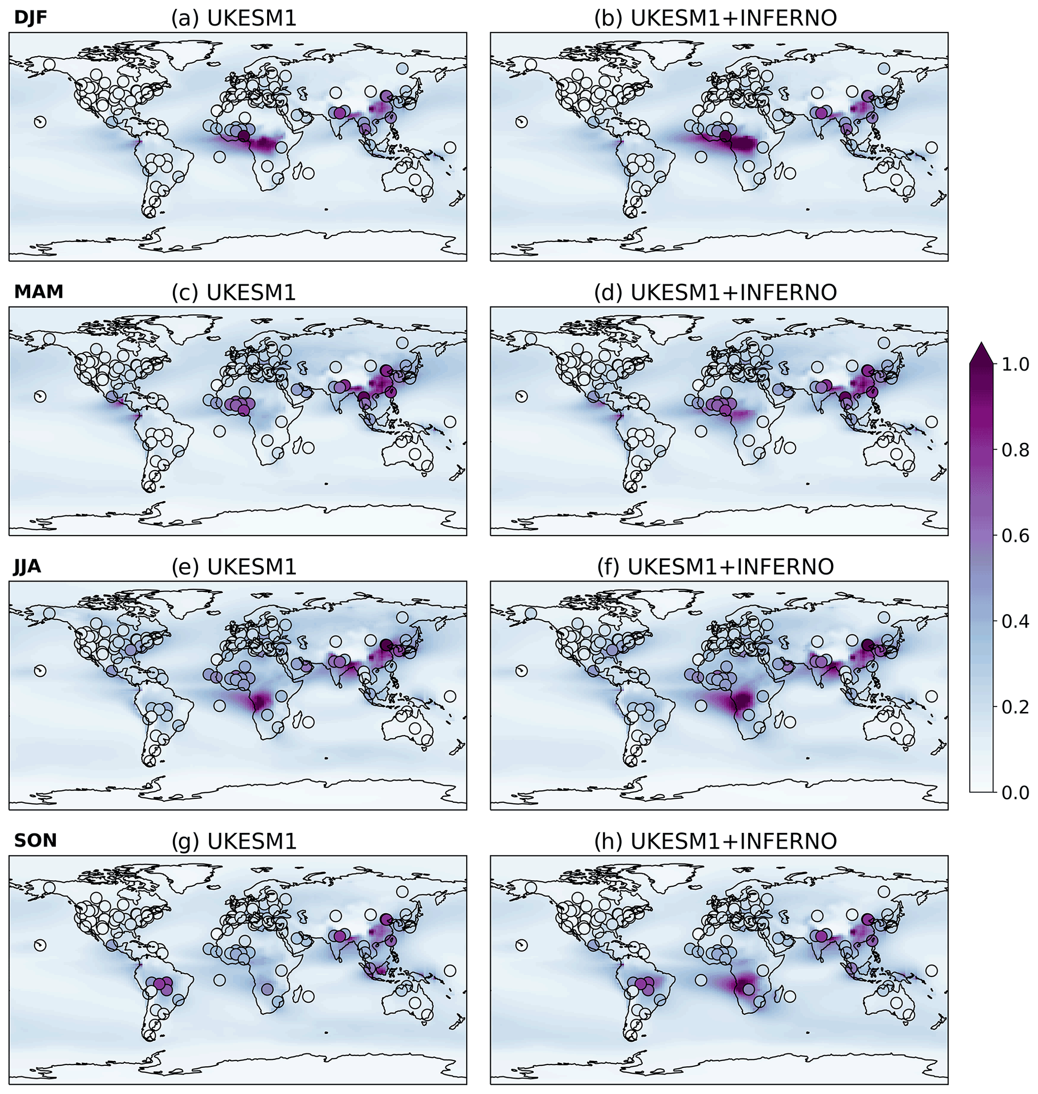
Figure 13Aerosol optical depth mean seasonal average at 440 nm (1980–2014) for the climatological seasons of DJF, MAM, JJA and SON (represented in each row) for UKESM1 (a, c, e, g) and UKESM1+INFERNO (b, d, f, h). The ground-based aerosol optical depth retrievals at various AERONET sites that have at least a 5-year overlapping period with model data are overlaid in circles using the same colour scale.
When comparing modelled AOD results with AERONET (Fig. 13), it is possible to see that these agree broadly with the analysis previously done for MODIS AOD. However, contrary to MODIS where UKESM1+INFERNO shows a negative bias, and possibly related to MODIS retrieval bias over bright surfaces, stations located in NHAF suggest that the model performs well during the boreal winter (DJF) (Fig. 13b) and underestimates the AOD for spring (MAM) (Fig. 13d). Moreover, for this region, there is a higher AOD during MAM for UKESM1+INFERNO (Fig. 13d) than for UKESM1 (Fig. 13c), bringing this model configuration closer to the AOD values found for the nearby AERONET station. On a similar note, for the SHAF region, there is also a better agreement between UKESM1+INFERNO and the AERONET AOD during the SON season (Fig. 13h), with UKESM1 (Fig. 13g) showing a negative bias relative to the stations found for this region. As seen before for South America (both NHSA and SHSA), both model configurations exhibit similar performance and show similar biases when comparing to MODIS – an overall underestimation of the AOD over these regions during the biomass burning season (SON).
Further to the differences introduced by the INFERNO interactive biomass burning emissions in UKESM1+INFERNO described previously, a different approach to the one adopted in UKESM1 has been taken regarding the vertical distribution of these emissions. For consistency between the approach regarding gas-phase biomass burning emissions, in UKESM1+INFERNO, these are injected into the model's lowest layer. However, while in UKESM1 prescribed aerosol biomass burning emissions are distributed uniformly over the 20 first model levels (∼3 km), in UKESM1+INFERNO these emissions are distributed following an exponential increasing with height function from the first model level to the 20th model level. In order to evaluate the vertical profile of modelled aerosol, the CALIPSO lidar level 3 aerosol extinction coefficient profiles product at 532 nm were used. Following the analysis of previous sections, we focused this analysis on the African (NHAF and SHAF) and South American (NHSA and SHSA) regions.
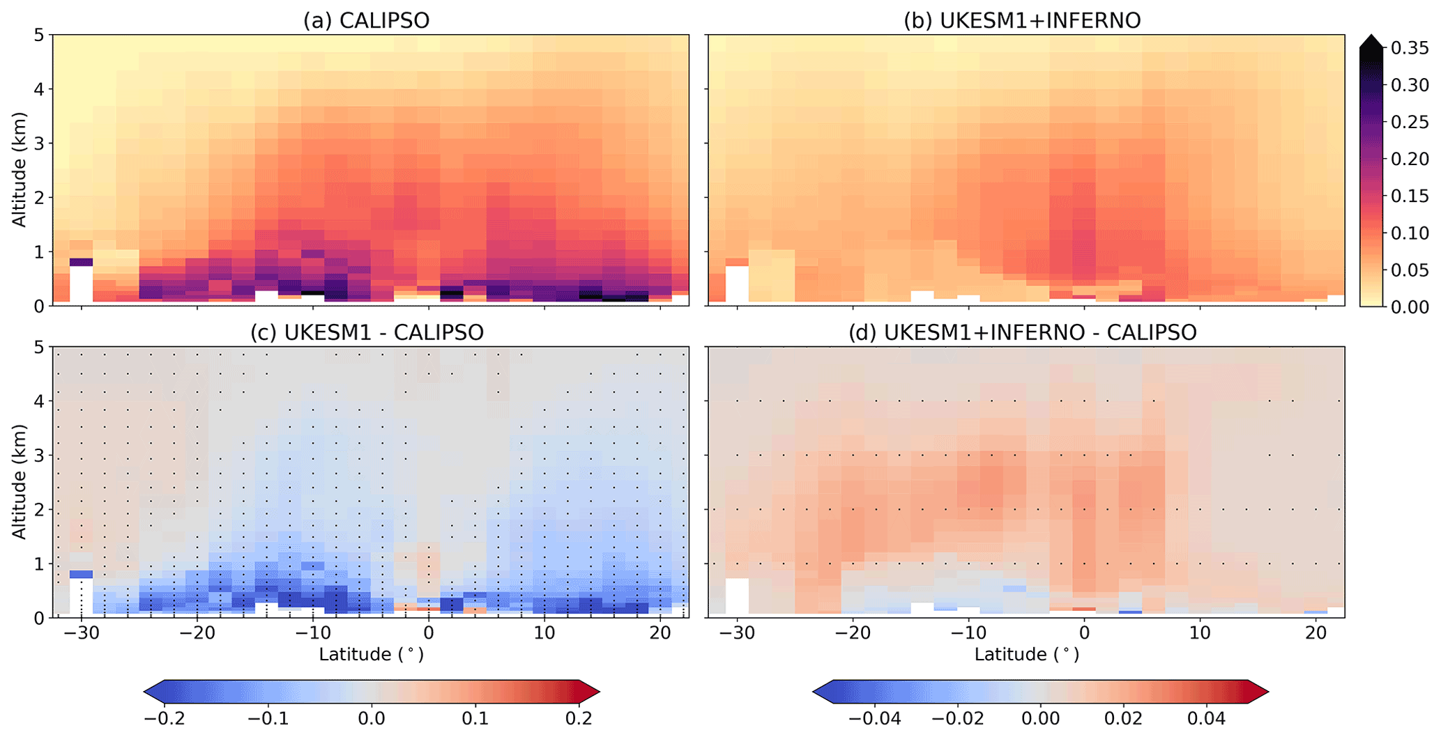
Figure 14Aerosol extinction coefficient mean (km−1) annual average vertical cross section at 532 nm (2006–2014) covering the African continent (extending both NHAF and SHAF regions) for (a) CALIPSO, (b) UKESM1+INFERNO, (c) difference between UKESM1 and CALIPSO, and (d) difference between UKESM1+INFERNO and UKESM1. Stapling is shown for points where the differences are statistically significant with a 95 % confidence level.
Over Africa – Fig. 14a – CALIPSO shows larger extinction coefficient in the first kilometre of the atmosphere, extending vertically up to 5 km over the tropical regions (5–15∘ N in latitude), associated with the vertical transport of aerosols. There are two main areas of large extinction coefficients: one associated with dust aerosol emissions from the Sahel region – down to ∼10∘ N as well as the southern edge biomass burning emission of NHAF extending further down to 0∘ N – and a second area from −5∘ N extending south to −25∘ N associated with the SHAF fire region. When comparing the model to CALIPSO (Fig. 14c and d), it can be seen that both of these model configurations show identical differences. On the lower levels (for altitudes below 1 km), there are significant large negative biases (>75 % compared to CALIPSO), except for biomass burning area around 0∘ N, where there is a small overestimation (<10 %). These lower-level biases also affect higher levels as aerosol are transported vertically. However, for altitudes above 1 km over the regions of the large negative bias, there is a reduction to 25 %–50 % when compared to CALIPSO. In addition, for latitudes below −25∘ N, the models result show a positive bias (<0.05 km−1), extending from 1 to 5 km in the vertical.
When comparing the extinction coefficient vertical profile of UKESM1+INFERNO to UKESM1 – Fig. 14d – it can be seen that the differences are 1 order of magnitude smaller than those found when comparing UKESM1+INFERNO to CALIPSO. UKESM1+INFERNO shows larger values of extinction coefficient at higher levels (above 1.5 km) and smaller at the lower levels (below 1.5 km) when compared to UKESM1 (Fig. 14c); this could be both an impact of the different treatment of emissions in the vertical, as well as due to transport associated with different locations for the biomass burning emissions. In addition, and as discussed before, due to the further extension towards south of the SHAF fire region, there is a positive bias throughout the vertical levels for latitudes southward of −20∘ N.
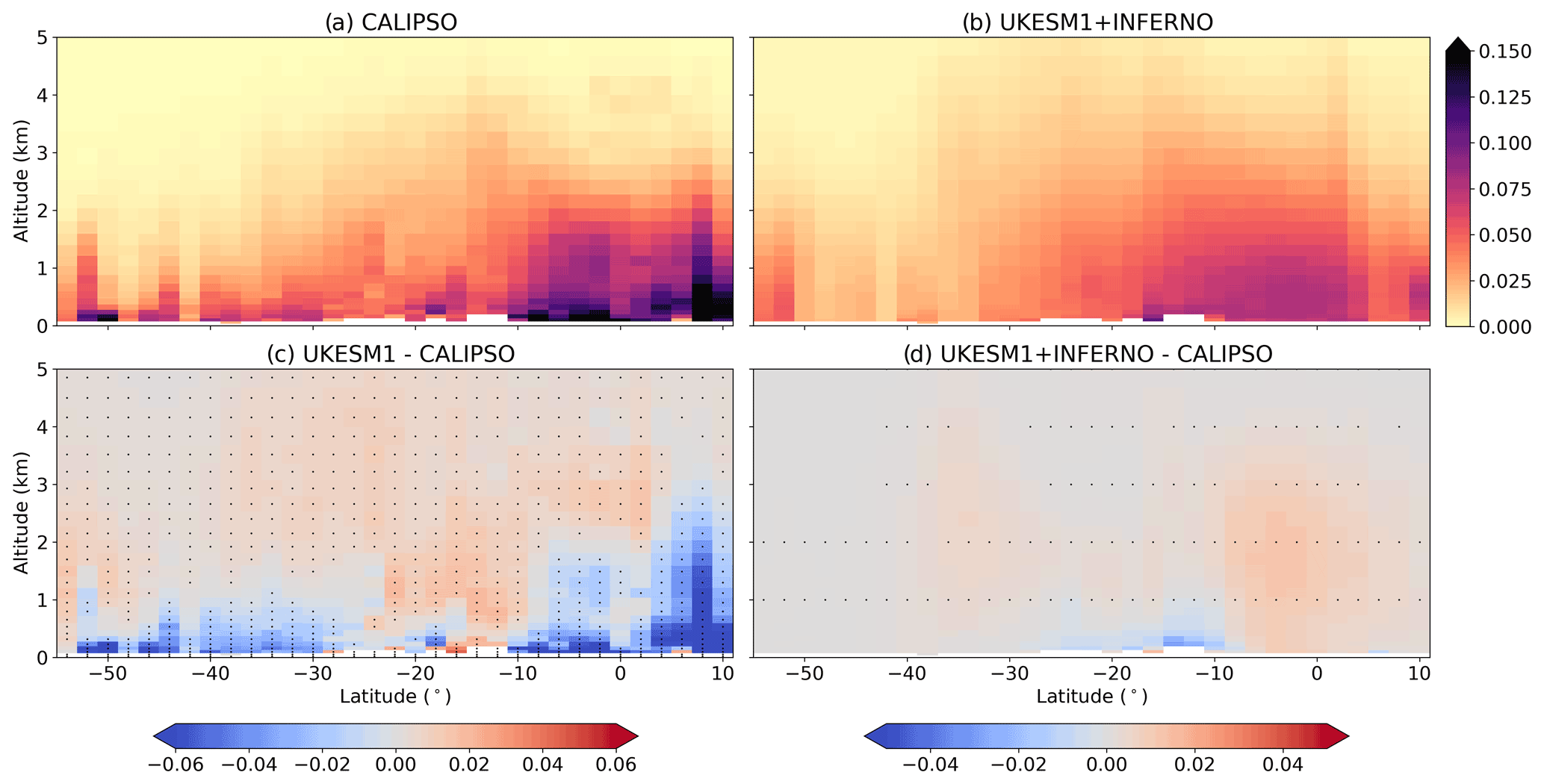
Figure 15Aerosol extinction coefficient mean annual average vertical cross section at 532 nm (2006–2014) covering the South American continent (extending both NHSA and SHSA regions) for (a) CALIPSO, (b) UKESM1+INFERNO, (c) difference between UKESM1 and CALIPSO, and (d) difference between UKESM1+INFERNO and UKESM1. Stapling is shown for points where the differences are statistically significant with a 95 % confidence level.
Similar results can be found when comparing UKESM1+INFERNO to CALIPSO for South America (Fig. 15). South American aerosol emissions are dominated by biomass burning, especially around tropical regions (−15 to 15∘ N). There is a large underestimation of the extinction coefficient for altitudes below 1 km (bias between 25 % and 50 % of the observed value). However, contrary to what could be seen for Africa, there is a positive bias for altitudes above 1 km (<0.02 km−1) in this region. When comparing UKESM1+INFERNO and UKESM1 – Fig. 15d – the difference is dominated by a large negative bias (∼25 % of the observed value in CALIPSO, as can be seen in Fig. 15a) between −25 and −5∘ N extending from the surface to an altitude of 4 km. This difference is consistent with the results found for AOD over this region, with UKESM1 (Fig. 15c) presenting a higher AOD when compared to UKESM1+INFERNO. This result, together with the differences between UKESM1+INFERNO and UKESM1 found for Africa, suggest that the influence of the underlying model bias in aerosol vertical and spatial distributions is dominant when compared to the influence of the different treatments of the vertical distribution of biomass burning aerosols.
The goal of this work was the development and evaluation of the implementation of a coupled fire–climate–composition ES model. This was built on top of the work developed by Mangeon et al. (2016), coupling the INFERNO fire model to the atmosphere-only configuration of version 1 of the UK's Earth System Model (UKESM1). The fire–atmosphere interactions through atmospheric chemistry and aerosols allow for fire emissions to provide feedback on radiation and clouds, changing weather, which can consequently provide feedback on the atmospheric drivers of fire. This is the basis for the development of a framework that would allow the impacts of fire variability on atmospheric composition–climate interactions in the past, present and future in an ES model context to be quantified. It also provides the possibility of adding further coupling to a dynamic land surface vegetation model in order to capture the fire–vegetation–atmospheric composition–climate interactions.
During the development of this work, it was identified that INFERNO human fire ignitions and fire suppression functions excluded the representation of socio-economic factors (aside from population) that can affect anthropogenic behaviour regarding fire ignitions. To address this, we include an HDI term aimed at representing socio-economic factors impacting fire ignition and suppression. The HDI is calculated based on three indicators designed to capture the income, health and education dimensions of human development. Therefore, we assume this leads to a representation where if there is more effort in improving human development, there is also investment on higher fire suppression by the population. Furthermore, the biomass burning emissions factors were updated according to the work of Andreae (2019) to reflect the state-of-the-art knowledge available since the development of INFERNO and emissions for C2H6, C3H8, HCHO, MeCHO, Me2CO and DMS were also added to make the fire–composition coupling consistent between UKESM1 and UKESM1+INFERNO. One of the limitations of the current biomass burning emission coupling framework is that the vertical distribution of emissions is not dependent on the radiative power of fire events. Instead, all fire events apply the same treatment to distribute these emissions vertically in the atmospheric column – surface emissions for gas-phase emissions and a linear increasing profile for aerosol emissions. Nevertheless, the results presented here suggest that the background bias in aerosols outweighs the differences introduced by using a different emission profile (Figs. 14 and 15). Moreover, it was shown that INFERNO is highly sensitive to the underlying land surface types of the land surface provided to the model. The prescribed land surface types used in this configuration of UKESM1+INFERNO overestimates the tree fraction in savanna biomes, such as the southern Africa (SHAF) and the southern edge of the Amazon rain forest (SHSA), which decreased the potential average burnt area and increased the fuel available for combustion and emissions, causing notable changes to the fire seasonality. This highlights the importance of correctly simulating land cover and it suggests that including the coupling between fire and vegetation in this framework could significantly improve model results as it would allow fires to shape regional land cover.
The model has a realistic spatial distribution of the average burnt area at a continental scale. However, there is a large underestimation of the annual average burnt area of approximately 250 Mha due to the underestimation of fires in NHAF and SHAF caused by the overestimates in the tree fraction for these regions. This underestimation of burnt areas impacts the biomass burning emissions. Despite the overall global pattern for biomass burning emissions being well reproduced by the model, there is a large overestimation of the biomass burning emissions for all the emitted species on the southern edge of NHAF and SHAF, as well as the eastern SHSA side (difference of > 300 %). Furthermore, in the SHAF region, the emissions extend further south into the midlatitudes. At a global scale, the effects of the underestimation of burnt areas is compensated by the increased availability of carbon provided by the overestimation of the tree fraction, resulting in good agreement with the observations.
Comparing UKESM1+INFERNO to TES-AURA satellite CO product showed that, despite the overestimation of CO over NHAF and SHAF due to the bias in the emissions, UKESM1+INFERNO has a similar performance when compared to UKESM1. In fact, including the interactive biomass burning emissions improves the interannual CO atmospheric column variability and consequently its seasonality over the main biomass burning regions – Africa and South America. Similarly, for aerosols, the AOD results broadly agree with MODIS and AERONET observations. Most of the biases found for aerosols are also present in UKESM1 and are not associated with the interactive biomass burning emissions. When comparing UKESM1+INFERNO to the observed datasets, and taking into account the background bias found in UKESM1, it can be seen that there is an overestimation of AOD over the biomass burning regions in Africa and an improvement of the variability and seasonality of AOD in South America, with UKESM1+INFERNO presenting better correlation and lower bias than UKESM1 for SHSA. Nonetheless, UKESM1+INFERNO does not capture the spikes in AOD, or CO observed over SHSA during the period 2004 to 2007 and 2010 associated with the Amazonian fire events that generally occur in drought years often related to El Niño events. Capturing these specific events depends on the ability of the model to represent circulation regimes that lead to the drought during the simulated period, as well as the vegetation flammability and fire ignitions. When analysing the vertical profile of aerosol extinction coefficient comparing to CALIPSO data, it was possible to see that there is an underestimate of aerosols in the first kilometre of the atmosphere which is present both in UKESM1 and UKESM1+INFERNO. This suggests that this is an underlying bias of the UKESM1 configuration – not related to the coupling of biomass burning emissions. These results are consistent with the results found for AOD over these regions, where UKESM1 is found to have a higher AOD when compared to UKESM1+INFERNO. This result, together with the differences between UKESM1+INFERNO and UKESM1 found for Africa suggest that the underlying model biases regarding aerosol spatial distributions are dominant when compared to the different treatment of the vertical distribution of the biomass burning aerosols.
Despite the present limitations of the implementation of coupled fire–composition–climate processes in this framework, it is evident that the UKESM1+INFERNO demonstrates a similar performance in reproducing the distribution of aerosols and CO atmospheric column. This shows that UKESM1+INFERNO provides a useful coupling framework that allows an internally consistent representation of complex fire–atmospheric composition–climate complex interactions and feedbacks in the Earth system. With further work to improve the existent model errors and bias, such as the coupling the fire feedbacks to vegetation and representing peatland regions, UKESM1+INFERNO can provide a useful framework to quantify the impacts of fire variability on atmospheric composition–climate interactions in past, present and future climates.
Due to intellectual property right restrictions, we cannot provide the source code or documentation papers for the UM or JULES. The Met Office Unified Model is available for use under licence. A number of research organizations and national meteorological services use the UM in collaboration with the Met Office to undertake basic atmospheric process research, produce forecasts, develop the UM code, and build and evaluate Earth system models. For further information on how to apply for a licence, see http://www.metoffice.gov.uk/research/modelling-systems/unified-model (last access: 3 August 2020). JULES is available under licence free of charge. For further information on how to gain permission to use JULES for research purposes, see http://jules-lsm.github.io/access_req/JULES_access.html (last access: 3 August 2020).
Details of the simulations performed: UM–JULES simulations are compiled and run in suites developed using the Rose suite engine (http://metomi.github.io/rose/doc/html/index.html, Met Office, 2021) and scheduled using the cylc workflow engine (https://cylc.github.io/, https://doi.org/10.1109/MCSE.2019.2906593, Oliver et al., 2019). Both Rose and cylc are available under v3 of the GNU General Public License (GPL). In this framework, the suite contains the information required to extract and build the code as well as configure and run the simulations. Each suite is labelled with a unique identifier and is held in the same revision-controlled repository service in which we hold and develop the model code. This means that these suites are available to any licensed user of both the UM and JULES under the following suite IDs:
-
UKESM1+INFERNO – u-br451
-
T2G10 – u-br947
-
T2G59 – u-bs281
UKESM1 AMIP data are available through Earth System Grid Federation and they are available from https://doi.org/10.22033/ESGF/CMIP6.5853 (Ridley et al., 2019).
JCT led the writing of the paper and model development. All co-authors contributed to the simulation design, writing sections, performing evaluation and reviewing drafts of the paper.
Some authors are members of the editorial board of Geoscientific Model Development. The peer-review process was guided by an independent editor, and the authors have also no other competing interests to declare.
Publisher's note: Copernicus Publications remains neutral with regard to jurisdictional claims in published maps and institutional affiliations.
The authors would like to acknowledge the international community of UKCA users for all their efforts in developing and applying the model. In particular, we would like to acknowledge John A. Pyle, who pioneered the development of the UKCA project. We would also like to thank the UKESM core team for developing and maintaining UKESM1 and all those who have contributed to the development of this model. We would especially like to thank those who have contributed to the development of INFERNO, with a special thanks to Stéphane Mangeon for taking the first steps to develop INFERNO and the observational community, who have developed numerous datasets used in this paper to help evaluate the model. This research and João C. Teixeira, Gerd Folberth, Fiona M. O'Connor were supported by the BEIS/Defra Met Office Hadley Centre Climate Programme (grant no. GA01101) and the Horizon 2020 Framework Programme (CRESCENDO, grant no. 779366). Apostolos Voulgarakis was funded via the Leverhulme Centre for Wildfires, Environment and Society through the Leverhulme Trust, grant no. RC-2018-023.
This research has been supported by the BEIS/Defra Met Office Hadley Centre Climate Programme (grant no. GA01101).
This paper was edited by Samuel Remy and reviewed by two anonymous referees.
Akagi, S. K., Yokelson, R. J., Wiedinmyer, C., Alvarado, M. J., Reid, J. S., Karl, T., Crounse, J. D., and Wennberg, P. O.: Emission factors for open and domestic biomass burning for use in atmospheric models, Atmos. Chem. Phys., 11, 4039–4072, https://doi.org/10.5194/acp-11-4039-2011, 2011.
Aldersley, A., Murray, S. J., and Cornell, S. E.: Global and regional analysis of climate and human drivers of wildfire, Sci. Total Environ., 409, 3472–3481, https://doi.org/10.1016/j.scitotenv.2011.05.032, 2011.
Andela, N., Morton, D. C., Giglio, L., Paugam, R., Chen, Y., Hantson, S., van der Werf, G. R., and Randerson, J. T.: The Global Fire Atlas of individual fire size, duration, speed and direction, Earth Syst. Sci. Data, 11, 529–552, https://doi.org/10.5194/essd-11-529-2019, 2019.
Andreae, M. O.: Emission of trace gases and aerosols from biomass burning – an updated assessment, Atmos. Chem. Phys., 19, 8523–8546, https://doi.org/10.5194/acp-19-8523-2019, 2019.
Andreae, M. O. and Merlet, P.: Emission of trace gases and aerosols from biomass burning, Global Biogeochem. Cy., 15, 955–966, https://doi.org/10.1029/2000GB001382, 2001.
Andreae, M. O. and Rosenfeld, D.: Aerosol-cloud-precipitation interactions. Part 1. The nature and sources of cloud-active aerosols, Earth-Sci. Rev., 89, 13–41, https://doi.org/10.1016/j.earscirev.2008.03.001, 2008.
Aragão, L. E. O. C., Anderson, L. O., Fonseca, M. G., Rosan, T. M., Vedovato, L. B., Wagner, F. H., Silva, C. V. J., Silva Junior, C. H. L., Arai, E., Aguiar, A. P., Barlow, J., Berenguer, E., Deeter, M. N., Domingues, L. G., Gatti, L., Gloor, M., Malhi, Y., Marengo, J. A., Miller, J. B., Phillips, O. L., and Saatchi, S.: 21st Century drought-related fires counteract the decline of Amazon deforestation carbon emissions, Nat. Commun., 9, 1–12, https://doi.org/10.1038/s41467-017-02771-y, 2018.
Archibald, A. T., O'Connor, F. M., Abraham, N. L., Archer-Nicholls, S., Chipperfield, M. P., Dalvi, M., Folberth, G. A., Dennison, F., Dhomse, S. S., Griffiths, P. T., Hardacre, C., Hewitt, A. J., Hill, R. S., Johnson, C. E., Keeble, J., Köhler, M. O., Morgenstern, O., Mulcahy, J. P., Ordóñez, C., Pope, R. J., Rumbold, S. T., Russo, M. R., Savage, N. H., Sellar, A., Stringer, M., Turnock, S. T., Wild, O., and Zeng, G.: Description and evaluation of the UKCA stratosphere–troposphere chemistry scheme (StratTrop vn 1.0) implemented in UKESM1, Geosci. Model Dev., 13, 1223–1266, https://doi.org/10.5194/gmd-13-1223-2020, 2020.
Athanasopoulou, E., Rieger, D., Walter, C., Vogel, H., Karali, A., Hatzaki, M., Gerasopoulos, E., Vogel, B., Giannakopoulos, C., Gratsea, M., and Roussos, A.: Fire risk, atmospheric chemistry and radiative forcing assessment of wildfires in eastern Mediterranean, Atmos. Environ., 95, 113–125, https://doi.org/10.1016/j.atmosenv.2014.05.077, 2014.
Baker, K. R., Woody, M. C., Tonnesen, G. S., Hutzell, W., Pye, H. O. T., Beaver, M. R., Pouliot, G., and Pierce, T.: Contribution of regional-scale fire events to ozone and PM2.5 air quality estimated by photochemical modeling approaches, Atmos. Environ., 140, 539–554, https://doi.org/10.1016/j.atmosenv.2016.06.032, 2016.
Bali, K., Mishra, A. K., and Singh, S.: Impact of anomalous forest fire on aerosol radiative forcing and snow cover over Himalayan region, Atmos. Environ., 150, 264–275, https://doi.org/10.1016/j.atmosenv.2016.11.061, 2017.
Beer, R., Glavich, T. A., and Rider, D. M.: Tropospheric emission spectrometer for the Earth Observing System's Aura satellite, Appl. Opt., 40, 2356, https://doi.org/10.1364/ao.40.002356, 2001.
Best, M. J., Pryor, M., Clark, D. B., Rooney, G. G., Essery, R. L. H., Ménard, C. B., Edwards, J. M., Hendry, M. A., Porson, A., Gedney, N., Mercado, L. M., Sitch, S., Blyth, E., Boucher, O., Cox, P. M., Grimmond, C. S. B., and Harding, R. J.: The Joint UK Land Environment Simulator (JULES), model description – Part 1: Energy and water fluxes, Geosci. Model Dev., 4, 677–699, https://doi.org/10.5194/gmd-4-677-2011, 2011.
Bistinas, I., Harrison, S. P., Prentice, I. C., and Pereira, J. M. C.: Causal relationships versus emergent patterns in the global controls of fire frequency, Biogeosciences, 11, 5087–5101, https://doi.org/10.5194/bg-11-5087-2014, 2014.
Bowman, D. M. J. S., Balch, J. K., Artaxo, P., Bond, W. J., Carlson, J. M., Cochrane, M. A., D'Antonio, C. M., DeFries, R. S., Doyle, J. C., Harrison, S. P., Johnston, F. H., Keeley, J. E., Krawchuk, M. A., Kull, C. A., Marston, J. B., Moritz, M. A., Prentice, I. C., Roos, C. I., Scott, A. C., Swetnam, T. W., Van Der Werf, G. R., and Pyne, S. J.: Fire in the earth system, Science, 324, 481–484, https://doi.org/10.1126/science.1163886, 2009.
Bowman, K. W., Rodgers, C. D., Kulawik, S. S., Worden, J., Sarkissian, E., Osterman, G., Steck, T., Lou, M., Eldering, A., Shephard, M., Worden, H., Lampel, M., Clough, S., Brown, P., Rinsland, C., Gunson, M., and Beer, R.: Tropospheric Emission Spectrometer: Retrieval method and error analysis, IEEE T. Geosci. Remote, 44, 1297–1306, https://doi.org/10.1109/TGRS.2006.871234, 2006.
Burton, C., Betts, R., Cardoso, M., Feldpausch, T. R., Harper, A., Jones, C. D., Kelley, D. I., Robertson, E., and Wiltshire, A.: Representation of fire, land-use change and vegetation dynamics in the Joint UK Land Environment Simulator vn4.9 (JULES), Geosci. Model Dev., 12, 179–193, https://doi.org/10.5194/gmd-12-179-2019, 2019.
Carslaw, K. S., Boucher, O., Spracklen, D. V., Mann, G. W., Rae, J. G. L., Woodward, S., and Kulmala, M.: A review of natural aerosol interactions and feedbacks within the Earth system, Atmos. Chem. Phys., 10, 1701–1737, https://doi.org/10.5194/acp-10-1701-2010, 2010.
Christian, T. J., Kleiss, B., Yokelson, R. J., Holzinger, R., Crutzen, P. J., Hao, W. M., Saharjo, B. H., and Ward, D. E.: Comprehensive laboratory measurements of biomass-burning emissions: 1. Emissions from Indonesian, African, and other fuels, J. Geophys. Res.-Atmos., 108, 4719, https://doi.org/10.1029/2003jd003704, 2003.
Clark, D. B., Mercado, L. M., Sitch, S., Jones, C. D., Gedney, N., Best, M. J., Pryor, M., Rooney, G. G., Essery, R. L. H., Blyth, E., Boucher, O., Harding, R. J., Huntingford, C., and Cox, P. M.: The Joint UK Land Environment Simulator (JULES), model description – Part 2: Carbon fluxes and vegetation dynamics, Geosci. Model Dev., 4, 701–722, https://doi.org/10.5194/gmd-4-701-2011, 2011.
Cox, P. M.: Description of the “TRIFFID” Dynamic Global Vegetation Model, Hadley Centre Technical Note 24, Met Office, UK, 1–17, 2001.
Daniau, A. L., Goñi, M. F. S., Martinez, P., Urrego, D. H., Bout-Roumazeilles, V., Desprat, S., and Marlon, J. R.: Orbital-scale climate forcing of grassland burning in southern Africa, P. Natl. Acad. Sci. USA, 110, 5069–5073, https://doi.org/10.1073/pnas.1214292110, 2013.
Dintwe, K., Okin, G. S., and Xue, Y.: Fire-induced albedo change and surface radiative forcing in sub-Saharan Africa savanna ecosystems: Implications for the energy balance, J. Geophys. Res., 122, 6186–6201, https://doi.org/10.1002/2016JD026318, 2017.
Doerr, S. H. and Santín, C.: Global trends in wildfire and its impacts: Perceptions versus realities in a changing world, Philos. T. R. Soc. B, 371, 20150345, https://doi.org/10.1098/rstb.2015.0345, 2016.
Durack, P. J. and Taylor, K. E.: PCMDI AMIP SST and sea-ice boundary conditions version 1.1.3, Earth System Grid Federation [data set], https://doi.org/10.22033/ESGF/input4MIPs.1735, 2017.
Eyring, V., Bony, S., Meehl, G. A., Senior, C. A., Stevens, B., Stouffer, R. J., and Taylor, K. E.: Overview of the Coupled Model Intercomparison Project Phase 6 (CMIP6) experimental design and organization, Geosci. Model Dev., 9, 1937–1958, https://doi.org/10.5194/gmd-9-1937-2016, 2016.
Felsberg, A., Kloster, S., Wilkenskjeld, S., Krause, A., and Lasslop, G.: Lightning Forcing in Global Fire Models: The Importance of Temporal Resolution, J. Geophys. Res.-Biogeo., 123, 168–177, https://doi.org/10.1002/2017JG004080, 2018.
Ganteaume, A., Camia, A., Jappiot, M., San-Miguel-Ayanz, J., Long-Fournel, M., and Lampin, C.: A review of the main driving factors of forest fire ignition over Europe, Environ. Manage., 51, 651–662, https://doi.org/10.1007/s00267-012-9961-z, 2013.
Giglio, L., Randerson, J. T., and Van Der Werf, G. R.: Analysis of daily, monthly, and annual burned area using the fourth-generation global fire emissions database (GFED4), J. Geophys. Res.-Biogeo., 118, 317–328, https://doi.org/10.1002/jgrg.20042, 2013.
Gillett, N. P., Weaver, A. J., Zwiers, F. W., and Flannigan, M. D.: Detecting the effect of climate change on Canadian forest fires, Geophys. Res. Lett., 31, L18211, https://doi.org/10.1029/2004GL020876, 2004.
Granier, C., Lamarque, J. F., Mieville, A., Muller, J. F., Olivier J., Orlando, J., Peters, J., Petron, G., Tyndall, G., and Wallens, S.: POET, a database of surface emissions of ozone precursors, Earth System Grid Federation [data set], http://www.aero.jussieu.fr/projet/ACCENT/POET.php (last access: 8 October 2021), 2005.
Hantson, S., Arneth, A., Harrison, S. P., Kelley, D. I., Prentice, I. C., Rabin, S. S., Archibald, S., Mouillot, F., Arnold, S. R., Artaxo, P., Bachelet, D., Ciais, P., Forrest, M., Friedlingstein, P., Hickler, T., Kaplan, J. O., Kloster, S., Knorr, W., Lasslop, G., Li, F., Mangeon, S., Melton, J. R., Meyn, A., Sitch, S., Spessa, A., van der Werf, G. R., Voulgarakis, A., and Yue, C.: The status and challenge of global fire modelling, Biogeosciences, 13, 3359–3375, https://doi.org/10.5194/bg-13-3359-2016, 2016.
Heil, A., Kaiser, J. W., van der Werf, G. R., Wooster, M. J., Schultz, M. G., and van der Gon, H. D.: Assessment of the Real-Time Fire Emissions (GFASv0) by MACC, ECMWF Tech. Memo., 628, 1–47, 2010.
Hewitt, H. T., Copsey, D., Culverwell, I. D., Harris, C. M., Hill, R. S. R., Keen, A. B., McLaren, A. J., and Hunke, E. C.: Design and implementation of the infrastructure of HadGEM3: the next-generation Met Office climate modelling system, Geosci. Model Dev., 4, 223–253, https://doi.org/10.5194/gmd-4-223-2011, 2011.
Hirota, M., Holmgren, M., van Nes, E. H., and Scheffer, M.: Global Resilience of Tropical Forest, Science, 334, 232–235, https://doi.org/10.1126/science.1210657, 2011.
Hoesly, R. M., Smith, S. J., Feng, L., Klimont, Z., Janssens-Maenhout, G., Pitkanen, T., Seibert, J. J., Vu, L., Andres, R. J., Bolt, R. M., Bond, T. C., Dawidowski, L., Kholod, N., Kurokawa, J.-I., Li, M., Liu, L., Lu, Z., Moura, M. C. P., O'Rourke, P. R., and Zhang, Q.: Historical (1750–2014) anthropogenic emissions of reactive gases and aerosols from the Community Emissions Data System (CEDS), Geosci. Model Dev., 11, 369–408, https://doi.org/10.5194/gmd-11-369-2018, 2018.
Holben, B. N., Eck, T. F., Slutsker, I., Tanré, D., Buis, J. P., Setzer, A., Vermote, E., Reagan, J. A., Kaufman, Y. J., Nakajima, T., Lavenu, F., Jankowiak, I., and Smirnov, A.: AERONET - A federated instrument network and data archive for aerosol characterization, Remote Sens. Environ., 66, 1–16, https://doi.org/10.1016/S0034-4257(98)00031-5, 1998.
Holben, B. N., Tanré, D., Smirnov, A., Eck, T. F., Slutsker, I., Abuhassan, N., Newcomb, W. W., Schafer, J. S., Chatenet, B., Lavenu, F., Kaufman, Y. J., Vande Castle, J., Setzer, A., Markham, B., Clark, D., Frouin, R., Halthore, R., Karneli, A., O'Neill, N. T., Pietras, C., Pinker, R. T., Voss, K., and Zibordi, G.: An emerging ground-based aerosol climatology: Aerosol optical depth from AERONET, J. Geophys. Res.-Atmos., 106, 12067–12097, https://doi.org/10.1029/2001JD900014, 2001.
Hsu, N. C., Tsay, S. C., King, M. D., and Herman, J. R.: Aerosol properties over bright-reflecting source regions, IEEE T. Geosci. Remote, 42, 557–569, https://doi.org/10.1109/TGRS.2004.824067, 2004.
Huang, S., Liu, H., Dahal, D., Jin, S., Li, S., and Liu, S.: Spatial variations in immediate greenhouse gases and aerosol emissions and resulting radiative forcing from wildfires in interior Alaska, Theor. Appl. Climatol., 123, 581–592, https://doi.org/10.1007/s00704-015-1379-0, 2016.
Johnson, B. T., Haywood, J. M., Langridge, J. M., Darbyshire, E., Morgan, W. T., Szpek, K., Brooke, J. K., Marenco, F., Coe, H., Artaxo, P., Longo, K. M., Mulcahy, J. P., Mann, G. W., Dalvi, M., and Bellouin, N.: Evaluation of biomass burning aerosols in the HadGEM3 climate model with observations from the SAMBBA field campaign, Atmos. Chem. Phys., 16, 14657–14685, https://doi.org/10.5194/acp-16-14657-2016, 2016.
Kaiser, J. W., Heil, A., Andreae, M. O., Benedetti, A., Chubarova, N., Jones, L., Morcrette, J.-J., Razinger, M., Schultz, M. G., Suttie, M., and van der Werf, G. R.: Biomass burning emissions estimated with a global fire assimilation system based on observed fire radiative power, Biogeosciences, 9, 527–554, https://doi.org/10.5194/bg-9-527-2012, 2012.
Kloster, S., Mahowald, N. M., Randerson, J. T., and Lawrence, P. J.: The impacts of climate, land use, and demography on fires during the 21st century simulated by CLM-CN, Biogeosciences, 9, 509–525, https://doi.org/10.5194/bg-9-509-2012, 2012.
Kummu, M., Taka, M., and Guillaume, J. H. A.: Gridded global datasets for Gross Domestic Product and Human Development Index over 1990–2015, Sci. Data, 5, 1–15, https://doi.org/10.1038/sdata.2018.4, 2018.
Lasslop, G., Coppola, A. I., Voulgarakis, A., Yue, C., and Veraverbeke, S.: Influence of Fire on the Carbon Cycle and Climate, Current Climate Change Reports, 5, 112–123, https://doi.org/10.1007/s40641-019-00128-9, 2019.
Li, F., Lawrence, D. M., and Bond-Lamberty, B.: Impact of fire on global land surface air temperature and energy budget for the 20th century due to changes within ecosystems, Environ. Res. Lett., 12, 044014, https://doi.org/10.1088/1748-9326/aa6685, 2017.
Liousse, C., Penner, J. E., Chuang, C., Walton, J. J., Eddleman, H., and Cachier, H.: A global three-dimensional model study of carbonaceous aerosols, J. Geophys. Res.-Atmos., 101, 19411–19432, https://doi.org/10.1029/95jd03426, 1996.
López-Saldaña, G., Bistinas, I., and Pereira, J. M. C.: Global analysis of radiative forcing from fire-induced shortwave albedo change, Biogeosciences, 12, 557–565, https://doi.org/10.5194/bg-12-557-2015, 2015.
Mahowald, N., Ward, D. S., Kloster, S., Flanner, M. G., Heald, C. L., Heavens, N. G., Hess, P. G., Lamarque, J.-F., and Chuang, P. Y.: Aerosol Impacts on Climate and Biogeochemistry, Annu. Rev. Environ. Resour., 36, 45–74, https://doi.org/10.1146/annurev-environ-042009-094507, 2011.
Mangeon, S., Voulgarakis, A., Gilham, R., Harper, A., Sitch, S., and Folberth, G.: INFERNO: a fire and emissions scheme for the UK Met Office's Unified Model, Geosci. Model Dev., 9, 2685–2700, https://doi.org/10.5194/gmd-9-2685-2016, 2016.
Marengo, J. A., Tomasella, J., Alves, L. M., Soares, W. R., and Rodriguez, D. A.: The drought of 2010 in the context of historical droughts in the Amazon region, Geophys. Res. Lett., 38, L12703, https://doi.org/10.1029/2011GL047436, 2011.
Met Office: Rose suite engine, available at: http://metomi.github.io/rose/doc/html/index.html, last access: 8 October 2021.
Morgenstern, O., Braesicke, P., O'Connor, F. M., Bushell, A. C., Johnson, C. E., Osprey, S. M., and Pyle, J. A.: Evaluation of the new UKCA climate-composition model – Part 1: The stratosphere, Geosci. Model Dev., 2, 43–57, https://doi.org/10.5194/gmd-2-43-2009, 2009.
Mulcahy, J. P., Johnson, C., Jones, C. G., Povey, A. C., Scott, C. E., Sellar, A., Turnock, S. T., Woodhouse, M. T., Abraham, N. L., Andrews, M. B., Bellouin, N., Browse, J., Carslaw, K. S., Dalvi, M., Folberth, G. A., Glover, M., Grosvenor, D. P., Hardacre, C., Hill, R., Johnson, B., Jones, A., Kipling, Z., Mann, G., Mollard, J., O'Connor, F. M., Palmiéri, J., Reddington, C., Rumbold, S. T., Richardson, M., Schutgens, N. A. J., Stier, P., Stringer, M., Tang, Y., Walton, J., Woodward, S., and Yool, A.: Description and evaluation of aerosol in UKESM1 and HadGEM3-GC3.1 CMIP6 historical simulations, Geosci. Model Dev., 13, 6383–6423, https://doi.org/10.5194/gmd-13-6383-2020, 2020.
Myhre, G.: Radiative effect of surface albedo change from biomass burning, Geophys. Res. Lett., 32, L20812, https://doi.org/10.1029/2005GL022897, 2005.
O'Connor, F. M., Johnson, C. E., Morgenstern, O., Abraham, N. L., Braesicke, P., Dalvi, M., Folberth, G. A., Sanderson, M. G., Telford, P. J., Voulgarakis, A., Young, P. J., Zeng, G., Collins, W. J., and Pyle, J. A.: Evaluation of the new UKCA climate-composition model – Part 2: The Troposphere, Geosci. Model Dev., 7, 41–91, https://doi.org/10.5194/gmd-7-41-2014, 2014.
Oliver, H., Shin, M., Matthews, D., Sanders, O., Bartholomew, S., Clark, A., Fitzpatrick, B., Van Haren, R., Drost, N., and Hut, R.: Workflow Automation for Cycling Systems, Comput. Sci. Eng., 21, 7–21, https://doi.org/10.1109/MCSE.2019.2906593, 2019 (data available at: https://cylc.github.io/, last access: 8 October 2021).
Pausas, J. G. and Keeley, J. E.: Abrupt Climate-Independent Fire Regime Changes, Ecosystems, 17, 1109–1120, https://doi.org/10.1007/s10021-014-9773-5, 2014.
Pechony, O. and Shindell, D. T.: Driving forces of global wildfires over the past millennium and the forthcoming century, P. Natl. Acad. Sci. USA, 107, 19167–19170, https://doi.org/10.1073/pnas.1003669107, 2010.
Pechony, O. and Shindell, D. T.: Fire parameterization on a global scale, J. Geophys. Res.-Atmos., 114, 1–10, https://doi.org/10.1029/2009JD011927, 2009.
Pezzatti, G. B., Zumbrunnen, T., Bürgi, M., Ambrosetti, P., and Conedera, M.: Fire regime shifts as a consequence of fire policy and socio-economic development: An analysis based on the change point approach, Forest Policy Econ., 29, 7–18, https://doi.org/10.1016/j.forpol.2011.07.002, 2013.
Price, C. and Rind, D.: Modeling global lightning distributions in a general circulation model, Mon. Weather Rev., 122, 1930–1939, https://doi.org/10.1175/1520-0493(1994)122<1930:MGLDIA>2.0.CO;2, 1994.
Rabin, S. S., Melton, J. R., Lasslop, G., Bachelet, D., Forrest, M., Hantson, S., Kaplan, J. O., Li, F., Mangeon, S., Ward, D. S., Yue, C., Arora, V. K., Hickler, T., Kloster, S., Knorr, W., Nieradzik, L., Spessa, A., Folberth, G. A., Sheehan, T., Voulgarakis, A., Kelley, D. I., Prentice, I. C., Sitch, S., Harrison, S., and Arneth, A.: The Fire Modeling Intercomparison Project (FireMIP), phase 1: experimental and analytical protocols with detailed model descriptions, Geosci. Model Dev., 10, 1175–1197, https://doi.org/10.5194/gmd-10-1175-2017, 2017.
Ramanathan, V. and Carmichael, G.: Global and regional climate changes due to black carbon, Nat. Geosci., 1, 221–227, https://doi.org/10.1038/ngeo156, 2008.
Randerson, J. T., Chen, Y., Van Der Werf, G. R., Rogers, B. M., and Morton, D. C.: Global burned area and biomass burning emissions from small fires, J. Geophys. Res.-Biogeo., 117, G04012, https://doi.org/10.1029/2012JG002128, 2012.
Rémy, S., Veira, A., Paugam, R., Sofiev, M., Kaiser, J. W., Marenco, F., Burton, S. P., Benedetti, A., Engelen, R. J., Ferrare, R., and Hair, J. W.: Two global data sets of daily fire emission injection heights since 2003, Atmos. Chem. Phys., 17, 2921–2942, https://doi.org/10.5194/acp-17-2921-2017, 2017.
Ridley, J., Menary, M., Kuhlbrodt, T., Andrews, M., and Andrews, T.: MOHC HadGEM3-GC31-LL model output prepared for CMIP6 CMIP amip. Version 20200803, Earth System Grid Federation [data set], https://doi.org/10.22033/ESGF/CMIP6.5853, 2019.
Rogers, B. M., Soja, A. J., Goulden, M. L., and Randerson, J. T.: Influence of tree species on continental differences in boreal fires and climate feedbacks, Nat. Geosci., 8, 228–234, https://doi.org/10.1038/ngeo2352, 2015.
Samset, B. H., Myhre, G., Herber, A., Kondo, Y., Li, S.-M., Moteki, N., Koike, M., Oshima, N., Schwarz, J. P., Balkanski, Y., Bauer, S. E., Bellouin, N., Berntsen, T. K., Bian, H., Chin, M., Diehl, T., Easter, R. C., Ghan, S. J., Iversen, T., Kirkevåg, A., Lamarque, J.-F., Lin, G., Liu, X., Penner, J. E., Schulz, M., Seland, Ø., Skeie, R. B., Stier, P., Takemura, T., Tsigaridis, K., and Zhang, K.: Modelled black carbon radiative forcing and atmospheric lifetime in AeroCom Phase II constrained by aircraft observations, Atmos. Chem. Phys., 14, 12465–12477, https://doi.org/10.5194/acp-14-12465-2014, 2014.
Sayer, A. M., Munchak, L. A., Hsu, N. C., Levy, R. C., Bettenhausen, C., and Jeong, M.-J.: MODIS Collection 6 aerosol products: Comparison between Aqua's e-Deep Blue, Dark Target, and “merged” data sets, and usage recommendations, J. Geophys. Res.-Atmos., 119, 13965–13989, https://doi.org/10.1002/2014JD022453, 2014.
Sellar, A. A., Jones, C. G., Mulcahy, J. P., Tang, Y., Yool, A., Wiltshire, A., O'Connor, F. M., Stringer, M., Hill, R., Palmieri, J., Woodward, S., de Mora, L., Kuhlbrodt, T., Rumbold, S. T., Kelley, D. I., Ellis, R., Johnson, C. E., Walton, J., Abraham, N. L., Andrews, M. B., Andrews, T., Archibald, A. T., Berthou, S., Burke, E., Blockley, E., Carslaw, K., Dalvi, M., Edwards, J., Folberth, G. A., Gedney, N., Griffiths, P. T., Harper, A. B., Hendry, M. A., Hewitt, A. J., Johnson, B., Jones, A., Jones, C. D., Keeble, J., Liddicoat, S., Morgenstern, O., Parker, R. J., Predoi, V., Robertson, E., Siahaan, A., Smith, R. S., Swaminathan, R., Woodhouse, M. T., Zeng, G., and Zerroukat, M.: UKESM1: Description and Evaluation of the U. K. Earth System Model, J. Adv. Model. Earth Sy., 11, 4513–4558, https://doi.org/10.1029/2019MS001739, 2019.
Sellar, A. A., Walton, J., Jones, C. G., Wood, R., Abraham, N. L., Andrejczuk, M., Andrews, M. B., Andrews, T., Archibald, A. T., Mora, L. De, Dyson, H., Elkington, M., Ellis, R., Florek, P., Good, P., Gohar, L., Haddad, S., Hardiman, S. C., Hogan, E., Iwi, A., Chris, D., Johnson, B., Kelley, D. I., Kettleborough, J., Jeff, R., Marcus, O. K., Kuhlbrodt, T., Liddicoat, S., Mizielinski, M. S., Morgenstern, O., Mulcahy, J., Neininger, E., Connor, F. M. O., Petrie, R., Ridley, J., Rioual, J., Roberts, M., Robertson, E., Seddon, J., Shepherd, H., Shim, S., and Stephens, A.: Implementation of UK Earth system models for CMIP6, J. Adv. Model. Earth Sy., 12, e2019MS001946, https://doi.org/10.1029/2019MS001946, 2020.
Settele, J., Scholes, R., Betts, R. A., Bunn, S., Leadley, P., Nepstad, D., Overpeck, J. T., Taboada, M. A., Fischlin, A., Moreno, J. M., Root, T., Musche, M., and Winter, M.: Terrestrial and Inland water systems, Clim. Chang. 2014 Impacts, Adapt. Vulnerability Part A Glob. Sect. Asp., Cambridge University Press, Cambridge, UK, 271–360, https://doi.org/10.1017/CBO9781107415379.009, 2015.
Sindelarova, K., Granier, C., Bouarar, I., Guenther, A., Tilmes, S., Stavrakou, T., Müller, J.-F., Kuhn, U., Stefani, P., and Knorr, W.: Global data set of biogenic VOC emissions calculated by the MEGAN model over the last 30 years, Atmos. Chem. Phys., 14, 9317–9341, https://doi.org/10.5194/acp-14-9317-2014, 2014.
Tackett, J. L., Winker, D. M., Getzewich, B. J., Vaughan, M. A., Young, S. A., and Kar, J.: CALIPSO lidar level 3 aerosol profile product: version 3 algorithm design, Atmos. Meas. Tech., 11, 4129–4152, https://doi.org/10.5194/amt-11-4129-2018, 2018.
Thomas, J. L., Polashenski, C. M., Soja, A. J., Marelle, L., Casey, K. A., Choi, H. D., Raut, J. C., Wiedinmyer, C., Emmons, L. K., Fast, J. D., Pelon, J., Law, K. S., Flanner, M. G., and Dibb, J. E.: Quantifying black carbon deposition over the Greenland ice sheet from forest fires in Canada, Geophys. Res. Lett., 44, 7965–7974, https://doi.org/10.1002/2017GL073701, 2017.
Unger, N. and Yue, X.: Strong chemistry-climate feedbacks in the Pliocene, Geophys. Res. Lett., 41, 527–533, https://doi.org/10.1002/2014GL061184, 2014.
van der Werf, G. R., Randerson, J. T., Giglio, L., Collatz, G. J., Mu, M., Kasibhatla, P. S., Morton, D. C., DeFries, R. S., Jin, Y., and van Leeuwen, T. T.: Global fire emissions and the contribution of deforestation, savanna, forest, agricultural, and peat fires (1997–2009), Atmos. Chem. Phys., 10, 11707–11735, https://doi.org/10.5194/acp-10-11707-2010, 2010.
van der Werf, G. R., Randerson, J. T., Giglio, L., van Leeuwen, T. T., Chen, Y., Rogers, B. M., Mu, M., van Marle, M. J. E., Morton, D. C., Collatz, G. J., Yokelson, R. J., and Kasibhatla, P. S.: Global fire emissions estimates during 1997–2016, Earth Syst. Sci. Data, 9, 697–720, https://doi.org/10.5194/essd-9-697-2017, 2017.
van Marle, M. J. E., Kloster, S., Magi, B. I., Marlon, J. R., Daniau, A.-L., Field, R. D., Arneth, A., Forrest, M., Hantson, S., Kehrwald, N. M., Knorr, W., Lasslop, G., Li, F., Mangeon, S., Yue, C., Kaiser, J. W., and van der Werf, G. R.: Historic global biomass burning emissions for CMIP6 (BB4CMIP) based on merging satellite observations with proxies and fire models (1750–2015), Geosci. Model Dev., 10, 3329–3357, https://doi.org/10.5194/gmd-10-3329-2017, 2017.
Vongruang, P., Wongwises, P., and Pimonsree, S.: Assessment of fire emission inventories for simulating particulate matter in Upper Southeast Asia using WRF-CMAQ, Atmos. Pollut. Res., 8, 921–929, https://doi.org/10.1016/J.APR.2017.03.004, 2017.
Voulgarakis, A. and Field, R. D.: Fire Influences on Atmospheric Composition, Air Quality and Climate, Current Pollution Reports, 1, 70–81, https://doi.org/10.1007/s40726-015-0007-z, 2015.
Voulgarakis, A., Telford, P. J., Aghedo, A. M., Braesicke, P., Faluvegi, G., Abraham, N. L., Bowman, K. W., Pyle, J. A., and Shindell, D. T.: Global multi-year O3-CO correlation patterns from models and TES satellite observations, Atmos. Chem. Phys., 11, 5819–5838, https://doi.org/10.5194/acp-11-5819-2011, 2011.
Voulgarakis, A., Marlier, M. E., Faluvegi, G., Shindell, D. T., Tsigaridis, K., and Mangeon, S.: Interannual variability of tropospheric trace gases and aerosols: The role of biomass burning emissions, J. Geophys. Res., 120, 7157–7173, https://doi.org/10.1002/2014JD022926, 2015.
Walters, D., Baran, A. J., Boutle, I., Brooks, M., Earnshaw, P., Edwards, J., Furtado, K., Hill, P., Lock, A., Manners, J., Morcrette, C., Mulcahy, J., Sanchez, C., Smith, C., Stratton, R., Tennant, W., Tomassini, L., Van Weverberg, K., Vosper, S., Willett, M., Browse, J., Bushell, A., Carslaw, K., Dalvi, M., Essery, R., Gedney, N., Hardiman, S., Johnson, B., Johnson, C., Jones, A., Jones, C., Mann, G., Milton, S., Rumbold, H., Sellar, A., Ujiie, M., Whitall, M., Williams, K., and Zerroukat, M.: The Met Office Unified Model Global Atmosphere 7.0/7.1 and JULES Global Land 7.0 configurations, Geosci. Model Dev., 12, 1909–1963, https://doi.org/10.5194/gmd-12-1909-2019, 2019.
Ward, D. S., Kloster, S., Mahowald, N. M., Rogers, B. M., Randerson, J. T., and Hess, P. G.: The changing radiative forcing of fires: global model estimates for past, present and future, Atmos. Chem. Phys., 12, 10857–10886, https://doi.org/10.5194/acp-12-10857-2012, 2012.
Westerling, A. L., Hidalgo, H. G., Cayan, D. R., and Swetnam, T. W.: Warming and earlier spring increase Western U.S. forest wildfire activity, Science, 313, 940–943, https://doi.org/10.1126/science.1128834, 2006.
Wilks, D. S.: Statistical methods in the atmospheric sciences, Elsevier/Academic Press, San Diego, USA, 2011.
Williams, K. D., Copsey, D., Blockley, E. W., Bodas-Salcedo, A., Calvert, D., Comer, R., Davis, P., Graham, T., Hewitt, H. T., Hill, R., Hyder, P., Ineson, S., Johns, T. C., Keen, A. B., Lee, R. W., Megann, A., Milton, S. F., Rae, J. G. L., Roberts, M. J., Scaife, A. A., Schiemann, R., Storkey, D., Thorpe, L., Watterson, I. G., Walters, D. N., West, A., Wood, R. A., Woollings, T., and Xavier, P. K.: The Met Office Global Coupled Model 3.0 and 3.1 (GC3.0 and GC3.1) Configurations, J. Adv. Model. Earth Sy., 10, 357–380, https://doi.org/10.1029/95JD00370, 2018.
Yienger, J. J. and Levy, H.: Empirical model of global soil-biogenic NOx emissions, J. Geophys. Res., 100, 11447–11464, https://doi.org/10.1029/95jd00370, 1995.