SITool (v1.0) – a new evaluation tool for large-scale sea ice simulations: application to CMIP6 OMIP

The Sea Ice Evaluation Tool (SITool) described in this paper is a performance metrics and diagnostics tool developed to evaluate the skill of Arctic and Antarctic model reconstructions of sea ice concentration, extent, edge location, drift, thickness, and snow depth. It is a Python-based software and consists of well-documented functions used to derive various sea ice metrics and diagnostics. Here, SITool version 1.0 (v1.0) is introduced and documented, and is then used to evaluate the performance of global sea ice reconstructions from nine models that provided sea ice output under the experimental protocols of the Coupled Model Intercomparison Project phase 6 (CMIP6) Ocean Model Intercomparison Project with two different atmospheric forcing datasets: the Coordinated Ocean-ice Reference Experiments version 2 (CORE-II) and the updated Japanese 55-year atmospheric reanalysis (JRA55-do). Two sets of observational references for the sea ice concentration, thickness, snow depth, and ice drift are systematically used to reflect the impact of observational uncertainty on model performance. Based on available model outputs and observational references, the ice concentration, extent, and edge location during 1980–2007, as well as the ice thickness, snow depth, and ice drift during 2003–2007 are evaluated. In general, model biases are larger than observational uncertainties, and model performance is primarily consistent compared to different observational references. By changing the atmospheric forcing from CORE-II to JRA55-do reanalysis data, the overall performance (mean state, interannual variability, and trend) of the simulated sea ice areal properties in both hemispheres, as well as the mean ice thickness simulation in the Antarctic, the mean snow depth, and ice drift simulations in both hemispheres are improved. The simulated sea ice areal properties are also improved in the model with higher spatial resolution. For the cross-metric analysis, there is no link between the performance in one variable and the performance in another. SITool is an open-access version-controlled software that can run on a wide range of CMIP6-compliant sea ice outputs. The current version of SITool (v1.0) is primarily developed to evaluate atmosphere-forced simulations and it could be eventually extended to fully coupled models.

1 Introduction

Most regional and global climate models now include an interactive sea ice model, reflecting the reality that sea ice plays a fundamental role in the polar environment, by influencing air–ice and ice–sea exchange, atmospheric and oceanic processes, and climate change. Large inter-model spread exists in the performance of sea ice simulations in the Coupled Model Intercomparison Project phase 5 (CMIP5) for both the Arctic and Antarctic (Massonnet et al., 2012; Stroeve et al., 2012, 2014; Turner et al., 2013; Zunz et al., 2013; Shu et al., 2015). Some improvements are identified in the CMIP6 models: (1) a more realistic estimate of sea ice loss for a given amount of CO₂ emissions and global warming in the Arctic (Notz et al., 2020), (2) reduced inter-model spread in summer and winter ice area and improved ice concentration distribution in the Antarctic (Roach et al., 2020), and (3) lower inter-model spread in the mean state and trend of both the Arctic and Antarctic ice extents (Shu et al., 2020). However, sea ice projections and evaluations are still not systematic, and, to date, no tool allows precise tracking of sea ice model performance through time from one version to the next. The Earth System Model Evaluation Tool (ESMValTool) has been developed for routine evaluation of climate model simulations in CMIP including many components of the Earth system (Eyring et al., 2016, 2020). It is an efficient tool to obtain a broad view on the overall performance of a climate model, and it provides sea ice diagnostics on the ice concentration and extent, as well as relationships between sea ice variables. In addition to sea ice diagnostics, the Sea Ice Evaluation Tool (SITool) introduced in this paper provides systematic sea ice metrics for assessing large-scale sea ice simulations from various aspects.

SITool has been designed to describe inter-model differences quantitatively and to help teams managing various versions of a sea ice model, detecting bugs in newly developed versions, or tracking the time evolution of model performance. SITool quantifies the performance of sea ice model simulations by providing systematic and meaningful sea ice metrics and diagnostics on each sea ice variable with thorough comparisons to a set of observational references. Arctic and Antarctic performance metrics and diagnostics on ice coverage, drift, thickness, and snow depth are provided from seasonal to multi-decadal timescales whenever observational references are available. These sea ice metrics give a detailed view of sea ice state and highlight major deficiencies in the sea ice simulation. SITool is written in the open-source language Python and distributed under the Nucleus for European Modelling of the Ocean (NEMO) standard tools. SITool is provided with the reference code and documentation to make sure the final results are traceable and reproducible.

Here, SITool version 1.0 (v1.0) is applied to evaluate the performance of Arctic and Antarctic historical sea ice simulations under the experimental protocols of the CMIP6 Ocean Model Intercomparison Project (OMIP, Griffies et al., 2016). OMIP provides global ocean–sea ice model simulations with a prescribed atmospheric forcing, which gives us the opportunity to intercompare sea ice model performance under fully controlled conditions. In OMIP, two streams of experiments were carried out: OMIP1, forced by the Coordinated Ocean-ice Reference Experiments version 2 interannual forcing (CORE-II, Large and Yeager, 2009), and OMIP2, forced by the updated Japanese 55-year atmospheric reanalysis (JRA55-do, Tsujino et al., 2018). The OMIP protocol ensures a close experimental setup among the different models. Models were run with both atmospheric forcings, when possible, to identify and attribute the influences of changed atmospheric forcings on sea ice characteristics. Tsujino et al. (2020) and Chassignet et al. (2020) evaluated the impact of atmospheric forcing and horizontal resolution on the global ocean–sea ice model simulations based on the experimental protocols of OMIP provided by model groups participated in this intercomparison project. Their studies focused on the evaluation of ocean components from sea surface height, temperature, salinity, mixed layer depth, and kinetic energy to circulation changes. Some aspects of sea ice simulations are assessed in both hemispheres relative to an observational dataset. Tsujino et al. (2020) provide spatial maps of the 1980–2009 mean ice concentration and time series of ice extent in summer and winter, and Taylor diagrams of the interannual variations of ice extent under CORE-II and JRA55-do forcings. Chassignet et al. (2020) show spatial maps of the 1980–2018 mean ice concentration and ice thickness in summer and winter, and time series of annual mean ice extent and ice volume under different horizontal resolutions. In this paper, we focus on the sea ice in OMIP simulations available from the Earth System Grid Federation in a more systematic manner, including more sea ice variables (e.g., ice-edge location, snow depth, and ice drift). The performance metrics and diagnostics (spatial maps and/or time series diagrams) for each ice variable are provided compared to two sets of observational references when data are available to appreciate the importance of observational uncertainty in the assessment.

This paper is organized as follows. SITool (v1.0) with the details of sea ice metrics and diagnostics is described in Sect. 2. The CMIP6 OMIP models and observational references are introduced in Sect. 3. In Sect. 4, the application of SITool (v1.0) to CMIP6 OMIP and the results of the model performance are presented and discussed. Finally, conclusions and discussion are provided in Sect. 5. Appendix A presents some additional sea ice diagnostics. The source code of SITool (v1.0) used to assess the model skills is publicly available in the repository as shown in the “Code and data availability” section.

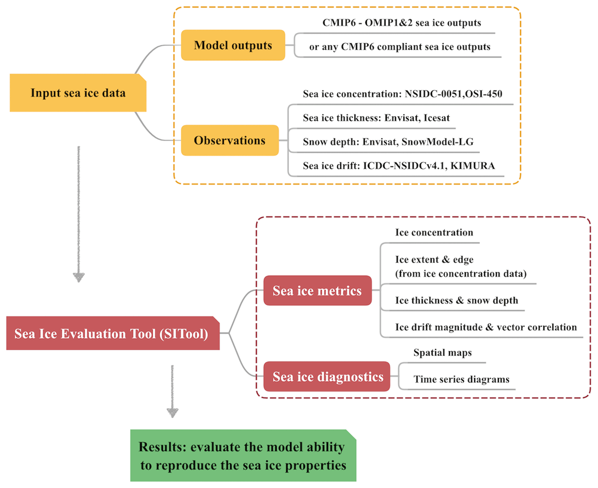
Figure 1 Schematic overview of SITool (v1.0) and its application to the CMIP6 OMIP model evaluation.

2 Overview of SITool (v1.0)

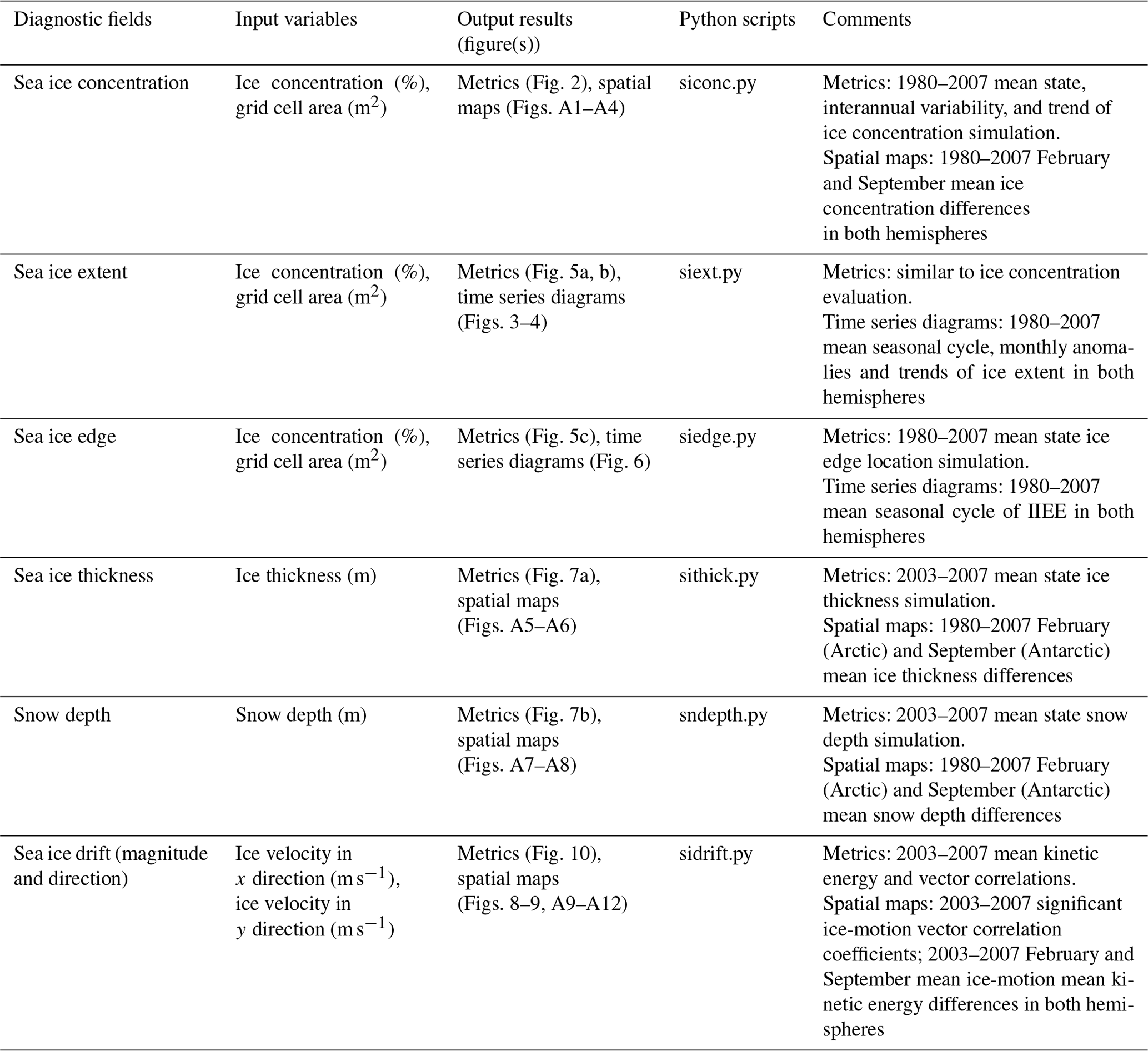
A schematic overview of SITool (v1.0) workflow and its application in evaluating the CMIP6 OMIP model performance is shown in Fig. 1. The input sea ice data from model outputs and observations are detailed in Sect. 3. The methods of the metrics calculation are discussed below in Sect. 2.1 followed Massonnet et al. (2011) with some modifications. Namely, (1) more observational references are used to calculate the observational errors, and the incorporation of observational errors is a prerequisite to do the comparisons here; (2) ice-edge location and snow depth metrics are included; (3) the method to calculate the vector correlation coefficient is updated. SITool (v1.0) also produces additional sea ice diagnostics (spatial maps and time series diagrams) to help understand why metrics vary from one dataset to the next. Table 1 provides an overview of the diagnostic fields along with input variables, output results and corresponding figures in this paper, Python scripts in the repository, and comments. All the sea ice data from model outputs and observational references are regridded to the polar stereographic 25 km resolution grid using a kd-tree (k-dimensional, Bentley, 1975) nearest-neighbor interpolation method provided by a Python package (a component of the SITool workflow). The kd tree is a binary search tree with a two-dimensional spatial index structure for use in this study. The interpolation yields less than 5 % error for each sea ice variable (not shown), which indicates that the results are not sensitive to the interpolation method used here. This interpolation allows point-by-point comparison and avoids the systematic bias of sea ice extent under different grids, due to differences in land–sea masks.

Table 1 Overview of the diagnostic fields along with input variables, output results and corresponding figures in this paper, Python scripts in the repository, and comments.

2.1 Sea ice metrics and diagnostics

The general approach to derive metrics is by computing scaled absolute errors. We first compute the errors (in absolute value) between some simulated characteristics (e.g., sea ice extent) in individual models and the corresponding characteristic in observational references, respectively. Then, we scale these errors by a typical error to finally get the corresponding metric. The typical error is defined as the absolute difference of the relevant characteristic between two observational references when observations are available and is therefore a proxy for observation uncertainty. Because our metrics are defined as scaled absolute errors, they are oriented positively meaning that lower values indicate better skill, and a value of 1 means that model error is comparable to observational uncertainty.

2.1.1 Sea ice concentration, extent, and edge location

The methods to calculate the metrics of ice concentration on the mean state, interannual variability, and trend in both hemispheres are introduced here. The consistent equations used to calculate the differences of the mean state (Meandiff), interannual variability (SDdiff), and trend (Trenddiff) between two datasets are shown below:

$$\begin{array}{}\text{(1)}& {\displaystyle }\mathrm{Meandiff}={\displaystyle \frac{{\sum }_{n=\mathrm{1}}^{n=\mathrm{12}}\left[\frac{{\sum }_{i=\mathrm{1}}^{i=N}|C_{\mathrm{0}\mathrm{M}}^{n,i}-C_{\mathrm{1}\mathrm{M}}^{n,i}|\times A_i}{{\sum }_{i=\mathrm{1}}^{i=N}{A}_i}\right]\times D_n}{{\sum }_{n=\mathrm{1}}^{n=\mathrm{12}}{D}_n}}\text{(2)}& {\displaystyle }\mathrm{SDdiff}={\displaystyle \frac{{\sum }_{i=\mathrm{1}}^{i=N}|\mathrm{SD}\left(C_{\mathrm{0}}^i-C_{\mathrm{0}\mathrm{M}}^i\right)-\mathrm{SD}\left(C_{\mathrm{1}}^i-C_{\mathrm{1}M}^i\right)\mathrm{|}\times A_i}{{\sum }_{i=\mathrm{1}}^{i=N}{A}_i}}\text{(3)}& {\displaystyle }\mathrm{Trenddiff}={\displaystyle \frac{\begin{array}{c}{\sum }_{i=\mathrm{1}}^{i=N}|\mathrm{trend}\left(C_{\mathrm{0}}^i-C_{\mathrm{0}\mathrm{M}}^i\right)\\ -\mathrm{trend}\left(C_{\mathrm{1}}^i-C_{\mathrm{1}\mathrm{M}}^i\right)|\times A_i\end{array}}{{\sum }_{i=\mathrm{1}}^{i=N}{A}_i}},\end{array}$$

where n=1, …, 12 and i=1, …, N denotes the 12 months and the grid cells, respectively, C_0M and C_1M are monthly mean ice concentrations from two datasets used to do the comparison, A and D are grid cell area and the days in each month, respectively, C₀ and C₁ are monthly ice concentrations from two datasets, and “SD” is the abbreviation of standard deviation. For the mean state evaluation, we compute the monthly mean ice concentration over the study period (1980–2007 for the CMIP6 OMIP model evaluation) and calculate the absolute difference between each model output and the observational reference over 12 months at each grid cell as shown in Eq. (1). For the interannual variability and trend evaluation, we compute the standard deviation and linear regression on the monthly anomalies of ice concentration over the study period and compute the absolute difference between each model output and the observational reference at each grid cell as shown in Eqs. (2) and (3). Then we average these errors spatially weighted by grid cell areas. The typical errors are the differences between two observational references on the mean state, interannual variability, and trend by applying the same method shown before. The differences between each model output and the observational reference are computed and scaled by corresponding typical errors to get the metrics on ice concentration. The September (February) mean ice concentration differences between each model output and the observational reference, and between two observational references in both hemispheres, are provided for diagnosis. These representative months of the summer and winter are selected because normally they, respectively, correspond to the minimum and maximum seasonal values of sea ice extent for both hemispheres in observations.

The ice extent is calculated as the total area of grid cells with the ice concentration above 15 %. The same procedure is followed for ice extent metrics calculation as for ice concentration, except for the spatial averaging since ice extent is already an integrated quantity. The mean seasonal cycle, monthly anomalies, and trend of ice extent in both hemispheres from different models and two observational references are provided for diagnosis.

The integrated ice-edge error (IIEE) is the total area where the models and observational references disagree on the ice concentration being above or below 15 % including both the ice extent error and a misplacement error (Goessling et al., 2016). For the mean IIEE evaluation, we compute the monthly mean IIEE between each model output and the observational reference over the study period. The typical error is the mean IIEE between two observational references themselves. The differences between each model output and the observational reference are computed and scaled by the typical error to get the metric on the ice-edge location. The mean seasonal cycles of IIEE between each model output and the observational reference, and between two observational references in both hemispheres, are provided for diagnosis.

2.1.2 Sea ice thickness and snow depth

The same procedure is followed for ice thickness and snow depth metrics calculation as for ice concentration, except for the spatial averaging with equal weight. For the CMIP6 OMIP model evaluation before 2007, the ice thickness and snow depth observations are limited to some months. Because the observational data are not complete to calculate differences between two observational references, the typical errors of ice thickness and snow depth are computed from the ice thickness and snow depth uncertainties of specific months from Envisat data. The mean winter (February for the Arctic and September for the Antarctic) ice thickness and snow depth from ESA's Environmental Satellite (Envisat) radar altimeter data and the differences between model outputs and Envisat data are provided for diagnosis in this study. The mean ice thickness and snow depth differences of other months in both hemispheres can be provided for diagnosis in the future during other study periods when observational references are available. This is not included in this study due to the limited observations for the evaluation before 2007.

2.1.3 Sea ice drift

The ice drift metrics include the evaluation of both the magnitude and direction of ice vectors by calculating the mean kinetic energy (MKE) and vector correlation of the ice vectors. The MKE is computed as

$$\begin{array}{}\text{(4)}& \mathrm{MKE}={\displaystyle \frac{\mathrm{1}}{\mathrm{2}}}\left(u^{\mathrm{2}}+v^{\mathrm{2}}\right),\end{array}$$

where u and v are zonal and meridional components of ice drift, respectively. For the MKE evaluation, we compute the monthly mean MKE over the study period and calculate the absolute difference between individual models and observational references over the 12 months at each grid cell. Then we average these errors spatially with equal weight. The typical error is the difference between two observational references of the MKE by applying the same method discussed before. The differences between each model output and the observational reference are computed and scaled by the typical error to get the metric on the ice drift magnitude.

The monthly mean ice vectors during the study period from individual models and observational references are correlated at each grid point by using a vector correlation measure, which is a generalization of the simple correlation coefficient between two scalar time series (Holland and Kwok, 2012). The vector correlation coefficient r² is computed by following the equations in Crosby et al. (1993), and the correlation coefficient is scaled (by a value of 2) to keep it between 0 and 1 in our study. The nr² follows the χ² distribution with 4 degrees of freedom, and the correlations are significant at a level of 99 % when nr²>8 with samples less than 64 based on the cumulative frequency distributions in Crosby et al. (1993). The significant correlation coefficients between individual models and observational references, and between two observational references are provided for diagnosis at each grid cell. Then we average these significant correlation coefficients spatially with equal weight. The typical correlation coefficient is a spatially averaged correlation coefficient between two observational references. As higher correlation coefficients indicate better skill, the typical correlation coefficients are scaled by the correlation coefficients between individual models and observational references to make it consistent with other metrics (lower values indicate better skill). The September (February) MKE differences and ice-motion vector correlation coefficients between each model output and the observational reference, and between two observational references in both hemispheres, are provided for diagnosis.

2.2 Models and observational references

In this study, SITool (v1.0) is used to evaluate the CMIP6 OMIP model skills in simulating the historical sea ice properties for both hemispheres. The CMIP6 OMIP models and a set of observational references providing ice concentration, thickness, snow depth, and ice drift are introduced in this section. Two sets of observational references for each sea ice variable are used for comparison.

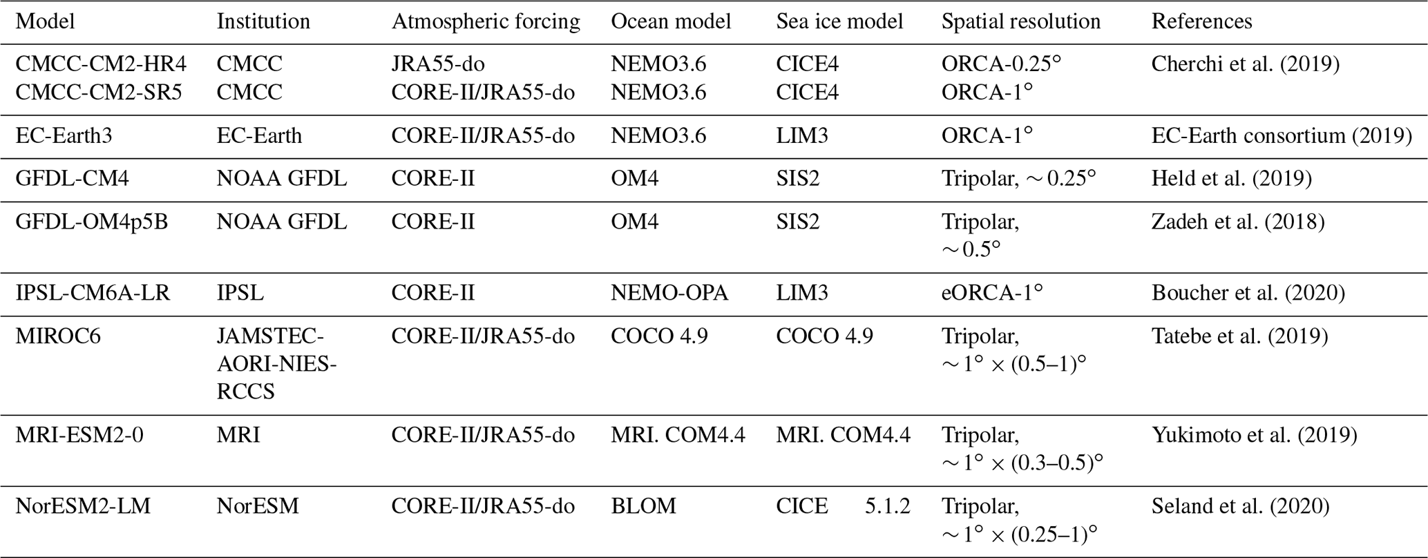
The CMIP6 OMIP models used are shown in Table 2 with model details such as atmospheric forcing, ocean models, sea ice models, spatial resolution, and related references. A major improvement in JRA55-do atmospheric forcing relative to the CORE-II forcing is the increased temporal frequency from 6 to 3 h and horizontal resolution from 1.875 to 0.5625^∘. The surface fields of JRA55-do forcing have been adjusted to match reference datasets based on high-quality satellite observations and several other atmospheric reanalysis products, as detailed in Tsujino et al. (2018). Nine models were run with either CORE-II or JRA55-do forcing; five of them were forced by both CORE-II and JRA55-do reanalysis; out of the four remaining models, one of them was forced by JRA55-do reanalysis only, and the other three were forced by CORE-II reanalysis only. The CMCC-CM2-HR4 (∼ 0.25^∘) and CMCC-CM2-SR5 (∼ 1^∘) models are different in spatial resolution, which provides an opportunity to identify the influence of model resolution on sea ice simulation. The CORE-II forcing dataset has not been updated since 2009 and the two Geophysical Fluid Dynamics Laboratory (GFDL) models only provide the model outputs until 2007. This is why the evaluation period is chosen as 1980–2007 for ice concentration, extent, and edge location (the corresponding observations are available from 1980). The evaluation period is 2003–2007 for ice thickness, snow depth, and ice drift because some observational references are limited before 2003, and then the corresponding metrics are only on the mean state. The evaluation period can be extended in the future when different model and observational datasets are considered.

Table 2 The details of nine CMIP6-OMIP models evaluated in the study.

The observational reference products for sea ice concentration, thickness, snow depth, and ice drift used to compare with model simulations are summarized in Table 3. The first ice concentration product derives from the passive microwave data of the Scanning Multichannel Microwave Radiometer (SMMR), the Special Sensor Microwave Imager (SSM/I), and the Special Sensor Microwave Imager/Sounder (SSMIS), which are processed by using the NASA Team algorithm (NSIDC-0051, Cavalieri et al., 1996). The other product is based on the same raw data but uses the EUMETSAT Ocean and Sea Ice Satellite Application Facility algorithm (OSI-450, Lavergne et al., 2019).

Table 3 Observational references used to compare with model simulations.

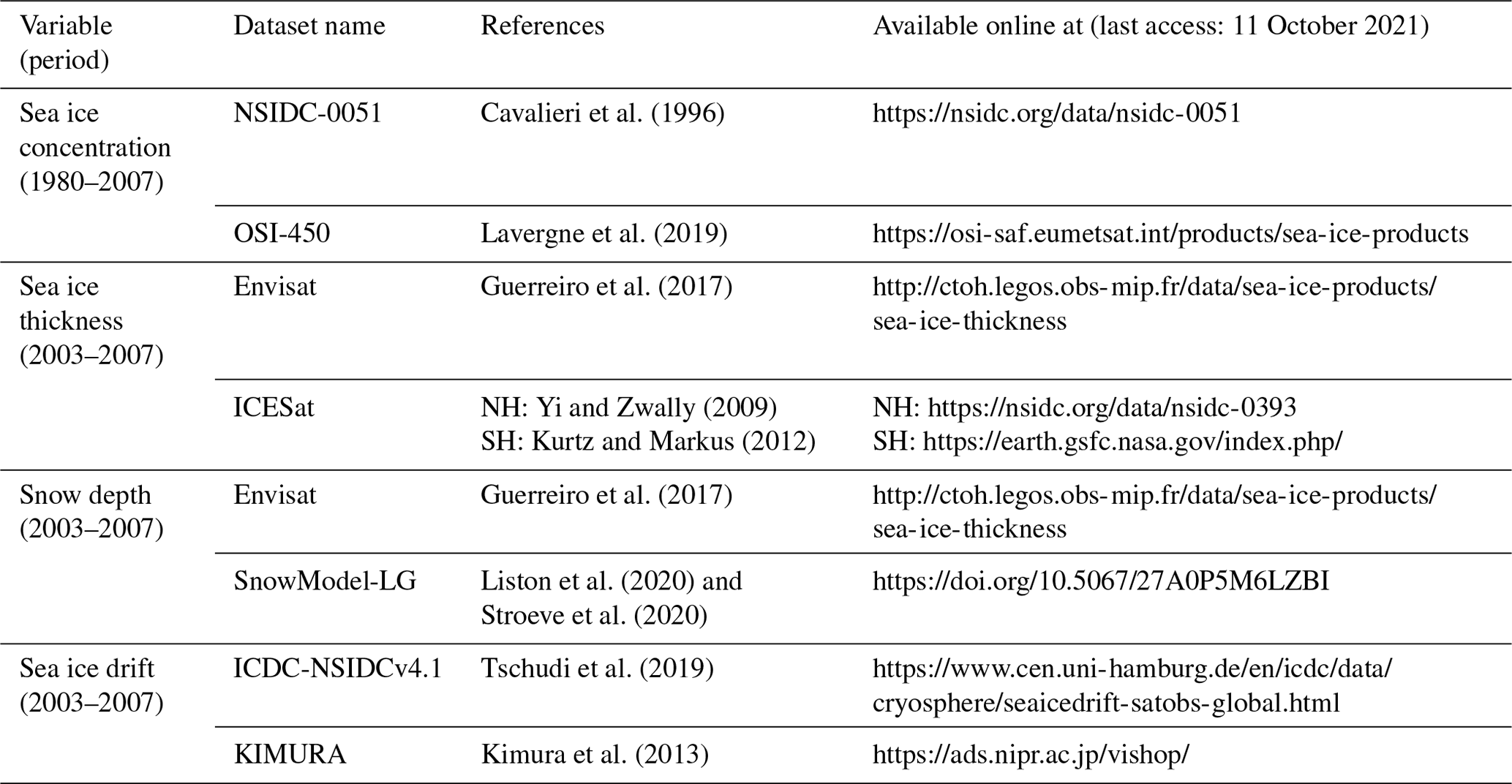
Our first ice thickness product is derived from the measurements of ESA's Envisat radar altimeter and provided by the Centre of Topography of Oceans and Hydrosphere (CTOH, Guerreiro et al., 2017). The other ice thickness product is from the measurements of the NASA's Ice, Cloud, and land Elevation Satellite (ICESat) Geoscience Laser Altimeter System (GLAS), and reprocessed separately for the Arctic (NSIDC-0393, Yi and Zwally, 2009) and Antarctic (Kurtz and Markus, 2012). The sea ice freeboard is less uncertain in observations than thickness; however, only five CMIP6 OMIP models at present provide sea ice freeboard, and the model's seawater densities, sea ice densities, and snow densities are not provided to calculate the freeboard. The Envisat data include ice thickness and thickness uncertainties from November to April for the Arctic with coverage up to 81.5^∘ N and May to October for the Antarctic from 2003. The ICESat data used here include 13 measurement campaigns for the Arctic and 11 for the Antarctic during 2003–2007, and these campaign periods are limited to the months of February–March, March–April, May–June, and October–November with each roughly 33 d. The comparisons between individual models and the two observational references are thus restricted to these months when data are available. The months chosen for the comparison are different from two ice thickness observational references, which can contribute to the differences in ice thickness performance metrics.

The Envisat thickness data also include snow depth and associated uncertainty. The other snow depth product derives from a Lagrangian snow-evolution model (SnowModel-LG) forced by the European Centre for Medium-Range Weather Forecasts (ECMWF) fifth-generation (ERA5) atmospheric reanalysis, and NSIDC sea ice concentration and trajectory datasets (Liston et al., 2020; Stroeve et al., 2020). The SnowModel-LG data are only provided for the Arctic Ocean. The SnowModel-LG data used to do the comparison are for the same months as the Envisat data from 2003–2007.

The first ice drift product is processed by NSIDC and enhanced by the Integrated Climate Data Center (ICDC-NSIDCv4.1). This product derives from SMMR, SSM/I, SSMIS, and the Advanced Very High Resolution Radiometer (AVHRR) for the Antarctic. In addition to the above data, data of the Advanced Multichannel Scanning Radiometer-Earth Observing System (AMSR-E), observations of the International Arctic Buoy Program (IABP), and ice drift derived from NCEP/NCAR surface winds are used for the Arctic Ocean. The second ice drift dataset is processed by Kimura et al. (2013) and derived from the AMSR-E data for both hemispheres from 2003.

The ice vectors are reprocessed before calculating the ice drift metrics. The ice vectors from observational references and models are rotated and interpolated to the polar stereographic grid. The monthly mean ice vectors of the observational references are computed when there are more than 10 d with valid daily drift data. The ICDC-NSIDCv4.1 ice drift data were shown to be biased low (i.e., too slow) relative to buoy data (Schwegmann et al. 2011; Barthélemy et al., 2018) and is therefore corrected by multiplying the drift components with a correction factor of 1.357 (Haumann et al., 2016). The ice vectors from observational references and models are removed when ice concentrations are below 50 %, or the data are closer than 75 km to the coast, or with a spurious value, to reduce the spatial and temporal noise by following Haumann et al. (2016).

3 SITool application and results

SITool (v1.0) described in Sect. 2 is applied in this section to assess the performance of the sea ice simulations for both hemispheres carried out under the CMIP6 OMIP1 and OMIP2 protocols. Models forced by CORE-II atmospheric reanalysis data (OMIP1) or JRA55-do reanalysis data (OMIP2) are marked as < model name + /C or /J >, respectively. The OMIP1 and OMIP2 model means shown below are from the five models of CMCC-CM2-SR5, EC-Earth3, MIROC6, MRI-ESM2-0, and NorESM2-LM, providing both OMIP1 and OMIP2 model outputs. All the sea ice data from models and observational references are interpolated to the NSIDC-0051 polar stereographic 25 km resolution grid for comparison. The typical errors are the differences between two observational references for the ice concentration, extent, edge location, and ice drift, while typical errors of ice thickness and snow depth are calculated from the thickness and snow depth uncertainties of specific months from Envisat data.

3.1 Sea ice concentration, extent, and edge location

Figure 2 shows that model errors on ice concentration simulations are around 2–5 times the observational uncertainty and the ice concentration simulations are much closer to the NSIDC-0051 data (Fig. 2a) compared to the OSI-450 data (Fig. 2b). In general, the overall ice concentration simulations (mean state, interannual variability, and trend) in both hemispheres are improved under OMIP2 protocol, forced by JRA55-do reanalysis. This is identified in Fig. 2a and b by comparing the five OMIP1 and OMIP2 model mean values (last two rows) and also by comparing five models' values separately under either OMIP protocol. The overall ice concentration simulations in both hemispheres are also improved in CMCC-CM2-HR4/J, with higher spatial resolution of ocean–sea ice model compared to CMCC-CM2-SR5/J (first and third rows). The improvements on the overall ice concentration simulations are not sensitive to the chosen observational reference and then robust. The improved ice concentration simulations are found compared to different observational references except for the interannual variability of the Antarctic ice concentration compared to the OSI-450 data as shown in the fifth column of Fig. 2b.

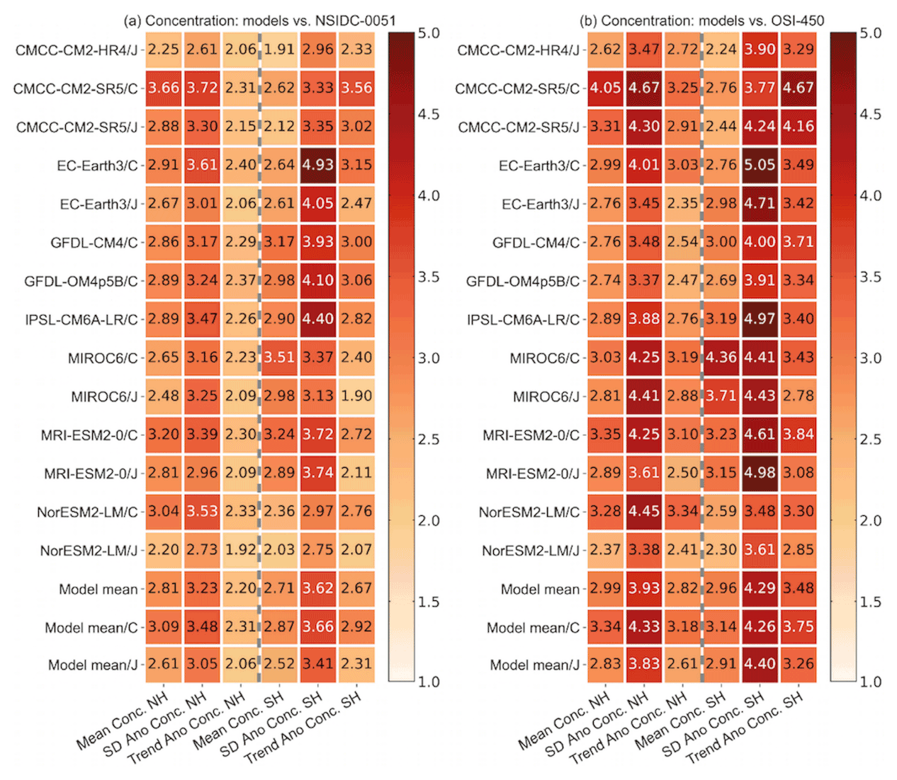
Figure 2 The ice concentration metrics of 14 model outputs under OMIP1 (/C) and OMIP2 (/J) protocols, 14-model mean (model mean), five-OMIP1-model mean (model mean/C), and five-OMIP2-model mean (model mean/J) from CMCC-CM2-SR5, EC-Earth3, MIROC6, MRI-ESM2-0, and NorESM2-LM compared to (a) NSIDC-0051 and (b) OSI-450 data. The six columns correspond to model performance metrics on the mean state, standard deviation (SD Ano), and trend (Trend Ano) of monthly anomalies of the Arctic and Antarctic ice concentration during 1980–2007. Lower values indicate better skill.

The metrics on the interannual variability of ice concentration (second and fifth columns) are the highest among all metrics, which indicates relatively lower skill on the simulation of ice concentration variability in both hemispheres compared to the mean state and trend. The overall best performance on ice concentration simulations including the mean state, interannual variability, and trend is in NorESM2-LM forced by JRA55-do reanalysis for both hemispheres. To help understand the differences in the ice concentration metrics, the 1980–2007 September and February mean ice concentration differences between the OSI-450 and NSIDC-0051 data, and between model outputs and the NSIDC-0051 data are produced for both hemispheres in Appendix A (Figs. A1–A4).

Figure 3a and b reveal that the monthly ice extent differences between two observational references (observational uncertainty, black × vs. cyan +) are much smaller compared to the model bias (red lines vs. black/cyan marks) in both hemispheres. The negative ice extent biases under OMIP1 protocol in the summer of both hemispheres are reduced under OMIP2 protocol (Fig. 3a and b, solid red vs. dash-dotted red) by changing the atmospheric forcing to JRA55-do reanalysis. The reduced mean ice extent biases in the summer under OMIP2 protocol are also identified in Tsujino et al. (2020) (see their Fig. 22 and Table D7). In the boreal winter, the five-model mean ice extents under OMIP1 and OMIP2 protocols show no obvious difference (Fig. 3a, solid red vs. dash-dotted red), and the ice extents among most models are close to the observational references (Fig. 3c) except for the MIROC6 (orange) and MRI-ESM2-0 (gray). In the austral winter, a large spread exists for the ice extent simulation (Fig. 3d), and the positive ice extent bias under OMIP1 protocol (Fig. 3b, solid red) becomes a negative one under OMIP2 protocol (dash-dotted red). The absolute value of ice extent bias in the austral winter under OMIP2 protocol is not reduced compared to that under OMIP1 protocol (Fig. 3b, dash-dotted red vs. solid red).

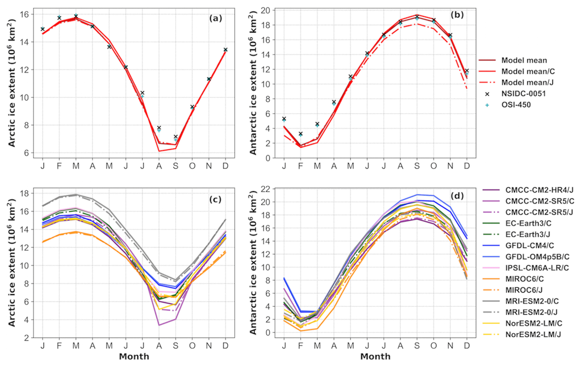
Figure 3 The 1980–2007 mean seasonal cycle of ice extent (10⁶ km²) from 14-model mean (solid brick red), five-model mean under OMIP1 and OMIP2 protocols (solid red and dash-dotted red), NSIDC-0051 (black ×), and OSI-450 (cyan +) in the (a) Arctic and (b) Antarctic. The five-model mean is from CMCC-CM2-SR5, EC-Earth3, MIROC6, MRI-ESM2-0, and NorESM2-LM. The mean seasonal cycle from 14 model outputs under OMIP1 (/C) and OMIP2 (/J) protocols are shown in panels (c) and (d), and the model outputs under OMIP2 protocol from the five models are in dash-dotted lines.

The biases of five-model mean ice extent monthly anomalies under OMIP1 protocol compared to the observational mean (solid green vs. solid black) are reduced under OMIP2 protocol (solid orange vs. solid black) in both hemispheres as shown in Fig. 4. The standard deviations of the monthly anomalies of ice extent in both hemispheres are smaller under OMIP2 protocol than that under OMIP1 protocol. In the Arctic (Fig. 4a and b), the negative biases of ice extent monthly anomalies during 1980–1982 and after 1998, as well as positive bias during 1986–1990, are reduced in the OMIP2 model mean (solid orange vs. solid green). However, the declining trend of ice extent from the observational mean (dashed black) is close to the OMIP1 model mean (dashed green) but not the OMIP2 model mean (dashed orange). This can be caused by the error compensation of the negative ice extent biases to observational mean during 1980–1982 and after 1998 in the OMIP1 model mean. In the Antarctic (Fig. 4c and d), the reduced bias is obvious after 1988 in the OMIP2 model mean (solid orange vs. solid green). The increasing trend of the Antarctic ice extent in the observational mean (dashed black) is not shown in the OMIP1 and OMIP2 mean (dashed green and dashed orange). The ice extent monthly anomalies in each model under OMIP1 and OMIP2 protocols are compared separately, and the improvements on the simulations of ice extent interannual variability are found in the OMIP2 model outputs of individual models (not shown). The improved interannual variability of ice extent in the OMIP2 simulations is also identified in Tsujino et al. (2020) (see their Figs. 22 and 23).

Figure 4 The 1980–2007 monthly anomalies of ice extent (10⁶ km²) from the observational mean of NSIDC-0051 and OSI-450 (solid black), five-model mean under OMIP1 or OMIP2 protocol (solid green vs. solid orange) in the Arctic (a, b) and Antarctic (c, d). The five-model mean is from CMCC-CM2-SR5, EC-Earth3, MIROC6, MRI-ESM2-0, and NorESM2-LM. The dashed lines are the trends computed from linear regression over 1980–2007. The standard deviation (SD, 10⁶ km²) and trend (10⁶ km² decade⁻¹) of the monthly anomalies of ice extent are computed and displayed.

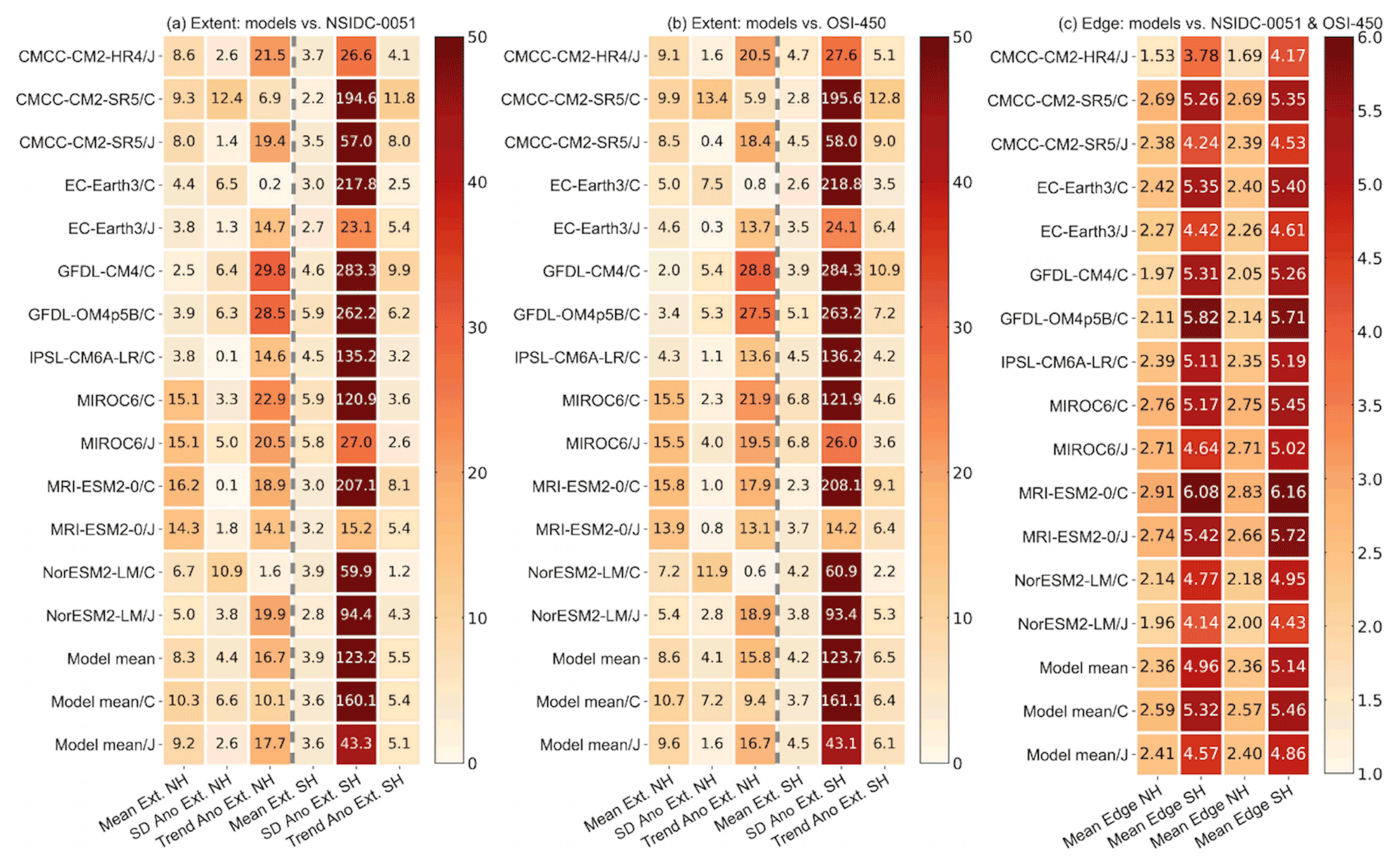
Figure 5 The ice extent metrics of 14 model outputs under OMIP1 (/C) and OMIP2 (/J) protocols, 14-model mean (model mean), five-OMIP1-model mean (model mean/C) and five-OMIP2-model mean (model mean/J) from CMCC-CM2-SR5, EC-Earth3, MIROC6, MRI-ESM2-0, and NorESM2-LM compared to (a) NSIDC-0051 and (b) OSI-450 data. The six columns correspond to model performance metrics on the mean state, standard deviation (SD Ano), and trend (Trend Ano) of monthly anomalies of the Arctic and Antarctic ice extent during 1980–2007. (c) The mean state ice-edge location metrics during 1980–2007 in both hemispheres compared to the NSIDC-0051 (first two columns) and OSI-450 data (last two columns). Lower values indicate better skill.

Figure 5a and b show that the model errors on ice extent simulation are much larger than the observational uncertainty in most cases, and the large values in the fifth columns are due to the very low typical error (0.0009×10⁶ km²) of the Antarctic interannual ice extent variability. In general, the ice extent simulations on the mean state and interannual variability for the Arctic, as well as the interannual variability and trend for the Antarctic, are improved under OMIP2 protocol, forced by JRA55-do reanalysis. This is identified in Fig. 5a and b by comparing the five OMIP1 and OMIP2 model mean values (last two rows), though there are several exceptions for the simulation of individual models under either OMIP protocol. The improved ice extent simulations are identified compared to different observational references.

The simulation of Arctic ice extent trend under OMIP2 protocol is not better than that under OMIP1 protocol (the third columns in Fig. 5a and b), which is due to the error compensation of the monthly anomalies biases of the ice extent during different periods under OMIP1 protocol as explained in Fig. 4a and b. This error compensation can change the trend and make it close to the observational references even though the monthly anomalies are not well presented in the OMIP1 models. The unimproved Antarctic mean ice extent under OMIP2 protocol can also be found in Fig. 3b, where the ice extent bias in the austral winter is not reduced under OMIP2 protocol. This is not consistent with what we found for the improvement in the ice concentration simulation under OMIP2 protocol, which is possibly because ice extent cancels out regional concentration differences. The overall best performance on ice extent simulation including the mean state, interannual variability, and trend is in EC-Earth3/C for the Arctic and in MRI-ESM2-0/J for the Antarctic.

To gain insights in the spatial distribution of errors, we then apply the IIEE (Goessling et al., 2016) as introduced in Sect. 2. In both hemispheres, the IIEEs between models and NSIDC-0051 are obviously much larger than that between two observational references as shown in Fig. 6. The largest model errors and model spread are in the summer of both hemispheres. The IIEE under OMIP1 protocol is much reduced under OMIP2 protocol especially in the summer of both hemispheres (Fig. 6a and b, solid red vs. dash-dotted red) by changing the atmospheric forcing to JRA55-do reanalysis. In both hemispheres, the large IIEE in CMCC-CM2-SR5/J (dashed light purple) is reduced in CMCC-CM2-HR4/J (solid dark purple) with higher spatial resolution of ocean–sea ice model during all the seasons (Fig. 6c and d). To identify the ice-edge location errors of various models, the contours of 15 % concentration derived from the 1980–2007 September and February mean ice concentration are also shown for both hemispheres in Appendix A (Figs. A1–A4).

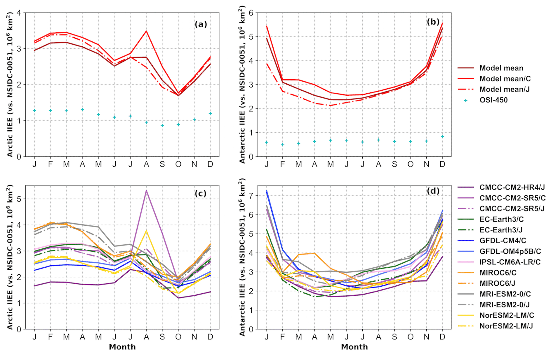
Figure 6 The 1980–2007 mean seasonal cycle of the integrated ice-edge error (IIEE; vs. NSIDC-0051, 10⁶ km²) from 14-model mean (solid brick red), five-model mean under OMIP1 and OMIP2 protocols (red solid and dash-dotted red), and OSI-450 (cyan +) in the (a) Arctic and (b) Antarctic. The five-model mean is from CMCC-CM2-SR5, EC-Earth3, MIROC6, MRI-ESM2-0, and NorESM2-LM. The mean seasonal cycle from 14 model outputs under OMIP1 (/C) and OMIP2 (/J) protocols are shown in panels (c) and (d), and the model outputs under OMIP2 protocol from the five models are in dash-dotted lines.

The mean state ice-edge location metrics in Fig. 5c show that model errors on ice-edge location simulations are around 2–6 times the observational uncertainty, and the ice-edge location simulations in the Arctic are much better than that in the Antarctic. Zampieri et al. (2019) also show that the prediction skill of sea-ice-edge location is 30 % lower in the Antarctic than in the Arctic from coupled subseasonal forecast systems. The lower prediction skill in the Antarctic can be related to more complicated ocean dynamic processes there, which decrease the persistence of ice areal changes (Ordoñez et al., 2018). The mean state ice-edge location simulations in both hemispheres are improved under OMIP2 protocol, which is identified in Fig. 5c by comparing the five-model mean values (last two rows) and also by comparing five models' values separately under either OMIP protocol. The mean state ice-edge location simulations in both hemispheres are also improved in CMCC-CM2-HR4/J with higher ocean–sea ice model resolution compared to CMCC-CM2-SR5/J (first and third rows). The improved ice-edge location simulations are identified compared to different observational references. The best performance on the mean state ice-edge location simulations is in CMCC-CM2-HR4/J for both hemispheres.

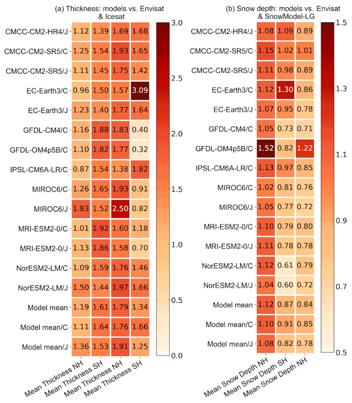
Figure 7 The mean state (a) ice thickness and (b) snow depth metrics during 2003–2007 of 14 model outputs under OMIP1 (/C) and OMIP2 (/J) protocols, 14-model mean (model mean), five-OMIP1-model mean (model mean/C) and five-OMIP2-model mean (model mean/J) from CMCC-CM2-SR5, EC-Earth3, MIROC6, MRI-ESM2-0, and NorESM2-LM. The four columns in (a) correspond to ice thickness metrics in both hemispheres compared to the Envisat (first two) and ICESat data (last two), and the three columns in (b) correspond to snow depth metrics compared to the Envisat data in both hemispheres (first two) and the SnowModel-LG data in the Arctic (last one). Lower values indicate better skill.

3.2 Sea ice thickness and snow depth

Figure 7 shows the mean state ice thickness and snow depth metrics, and the interannual variability and trend metrics are not included here because the observational record is too short to make such an assessment (Tilling et al., 2015). The model errors on the mean ice thickness and snow depth simulations are not obviously larger (even smaller in some models) than the observational uncertainty. The mean ice thickness simulation during 2003–2007 is improved in the Antarctic under OMIP2 protocol, forced by JRA55-do reanalysis. This is identified in Fig. 7a by comparing the five-model mean values (last two rows) and also by comparing the five models' values separately under either OMIP protocol (an exception in NorESM2-LM compared to the ICESat data). The improved Antarctic mean ice thickness simulations are identified compared to different observational references. The best performance on the mean ice thickness simulation is in IPSL-CM6A-LR/C for the Arctic, while for the Antarctic the best performance is in CMCC-CM2-HR4/J compared to the Envisat data and in GFDL-OM4p5B/C compared to the ICESat data. The different model performance on the mean ice thickness simulations by comparing to two observational references is due to the different months chosen for the ice thickness comparison.

The mean snow depth simulation during 2003–2007 in both hemispheres improved a bit under OMIP2 protocol, which can be found by comparing five-model mean values under either OMIP protocol (last two rows) in Fig. 7b. The improvement on the mean snow depth simulation is relatively small compared to other ice metrics. The best performance on the mean snow depth simulation for the Arctic is in MIROC6/C compared to the Envisat data and in GFDL-CM4/C compared to the SnowModel-LG data, and for the Antarctic, the best performance is in NorESM2-LM/J (Fig. 7b). To help understand the differences in the ice thickness and snow depth metrics, the 2003–2007 winter-mean ice thickness and snow depth from Envisat data, and the differences between model outputs and Envisat data, are produced for both hemispheres in Appendix A (Figs. A5–A8).

3.3 Sea ice drift

The magnitude and direction of simulated ice drifts are evaluated by calculating the MKE and the vector correlation from monthly mean ice-vector data during 2003–2007. The vector correlation coefficients are measured by using a generalization of the simple correlation coefficient between two scalar time series as introduced in Sect. 2. The significant correlation coefficient at a level of 99 % between ICDC-NSIDCv4.1 and KIMURA data, and between 14 model outputs and KIMURA data in the Arctic (Fig. 8) and Antarctic (Fig. 9) are displayed. The correlation coefficients are much lower between model outputs and the KIMURA data than that between two observational references. This is obvious for the coastal regions of Greenland and Canadian archipelago in the Arctic and the Weddell Sea and the Ross Sea in the Antarctic, as well as the ice-edge location of the Weddell Sea among some models. This implies that model errors on the ice-vector direction simulations are much larger than the observational uncertainty. The correlation coefficients are higher under OMIP2 protocol than that under OMIP1 protocol (third vs. second column in Figs. 8 and 9), which indicate the improvement on the ice-vector direction simulation when forced by JRA55-do atmospheric forcing in both hemispheres.

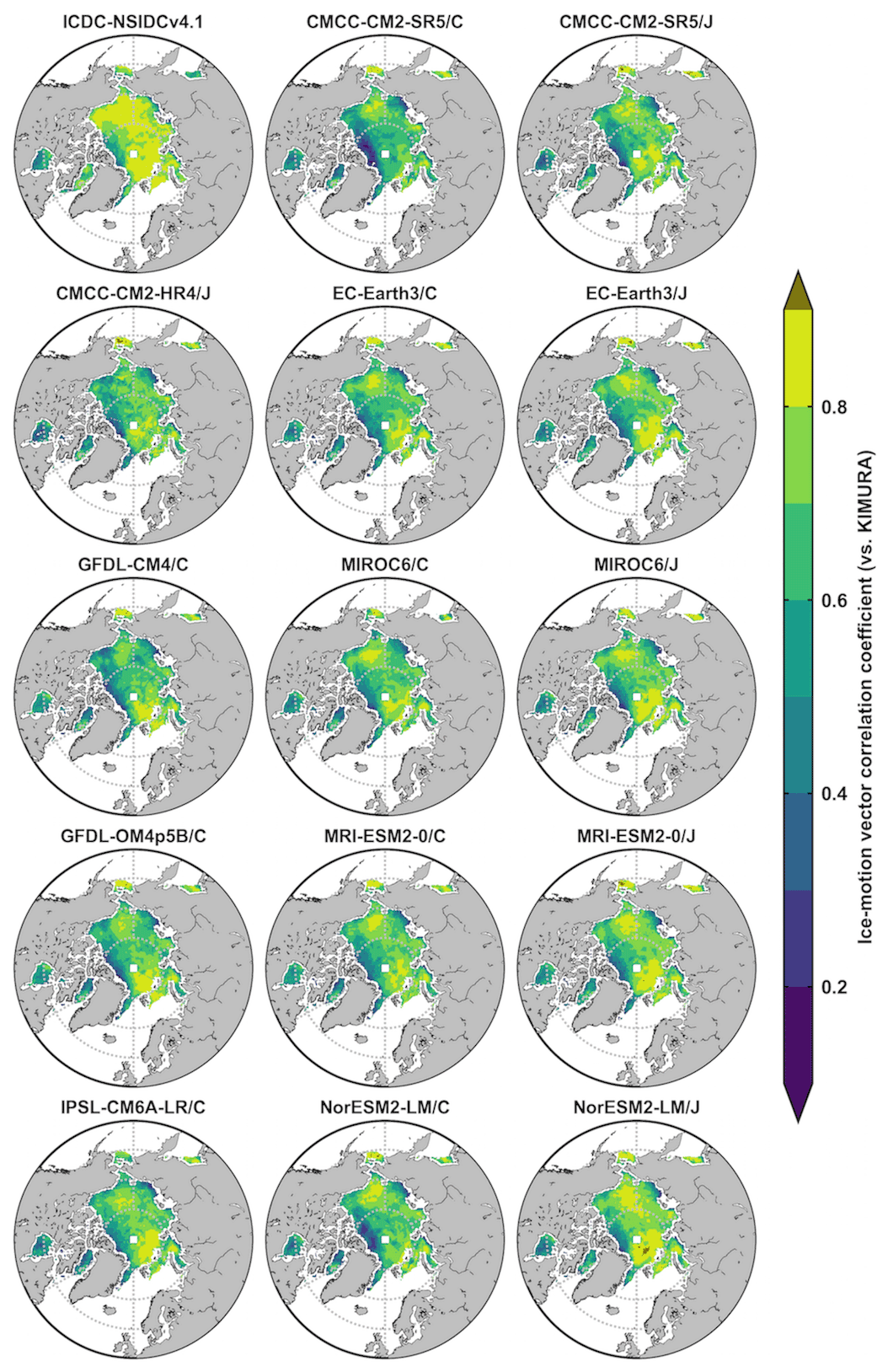
Figure 8 The significant Arctic ice-motion vector correlation coefficients from monthly mean data during 2003–2007 at a level of 99 % between ICDC-NSIDCv4.1/model outputs and the KIMURA data. The second and third columns are from the five OMIP1 and OMIP2 model outputs of CMCC-CM2-SR5, EC-Earth3, MIROC6, MRI-ESM2-0, and NorESM2-LM, respectively.

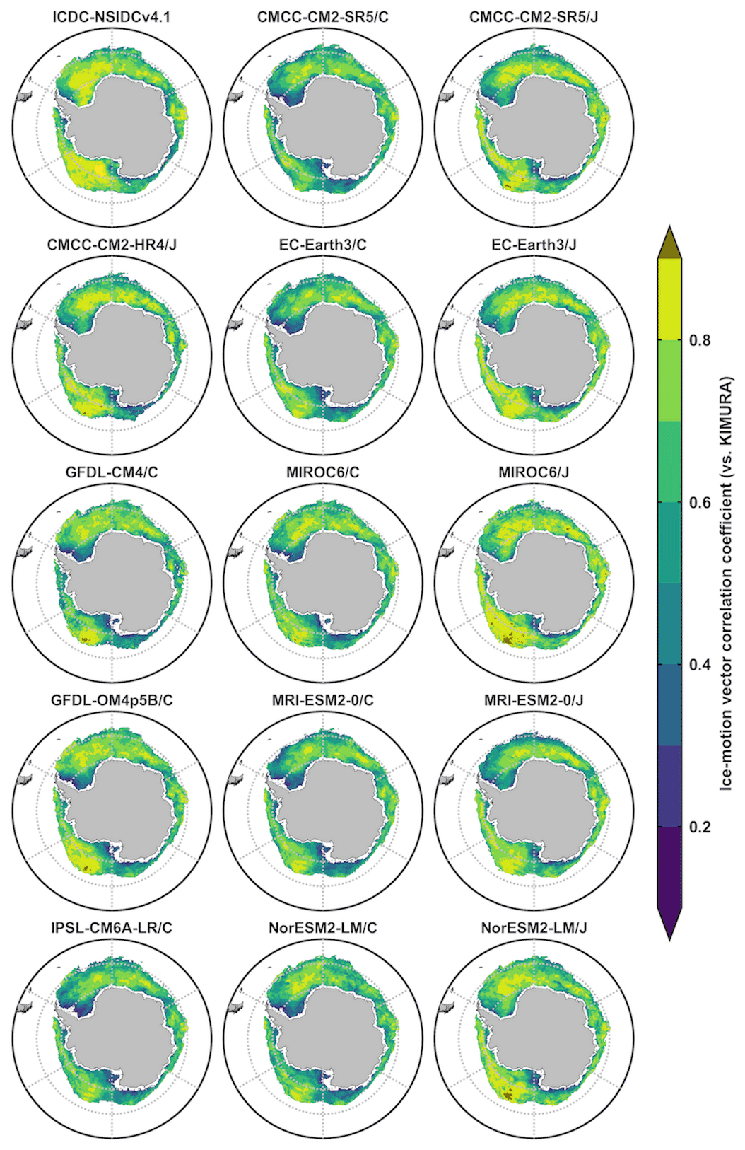
Figure 9 The significant Antarctic ice-motion vector correlation coefficients from monthly mean data during 2003–2007 at a level of 99 % between ICDC-NSIDCv4.1/model outputs and the KIMURA data. The second and third columns are from the five OMIP1 and OMIP2 model outputs of CMCC-CM2-SR5, EC-Earth3, MIROC6, MRI-ESM2-0, and NorESM2-LM, respectively.

Figure 10 shows that model errors on the mean ice drift simulations are larger than the observational uncertainty. In general, the ice drift simulations on the magnitude (Fig. 10a) and direction (Fig. 10b) in both hemispheres are improved under OMIP2 protocol, forced by JRA55-do reanalysis. This is identified from the five OMIP1 and OMIP2 model mean values (last two rows) and also by comparing five models' values separately under either OMIP protocol (an exception in CMCC-CM2-SR5 of the Arctic ice-vector magnitude in Fig. 10a). The improved mean ice drift simulations under OMIP2 protocol are found compared to not only the ICDC-NSIDCv4.1 data but also the KIMURA data. The overall best performance on sea ice drift simulations including the magnitude and direction is in MIROC6/J for both hemispheres. To help understand the differences in the ice-motion magnitude metrics, the 2003–2007 September and February mean ice-motion MKE differences between the ICDC-NSIDCv4.1 and KIMURA data, and between model outputs and the KIMURA data are produced for both hemispheres in Appendix A (Figs. A9–A12).

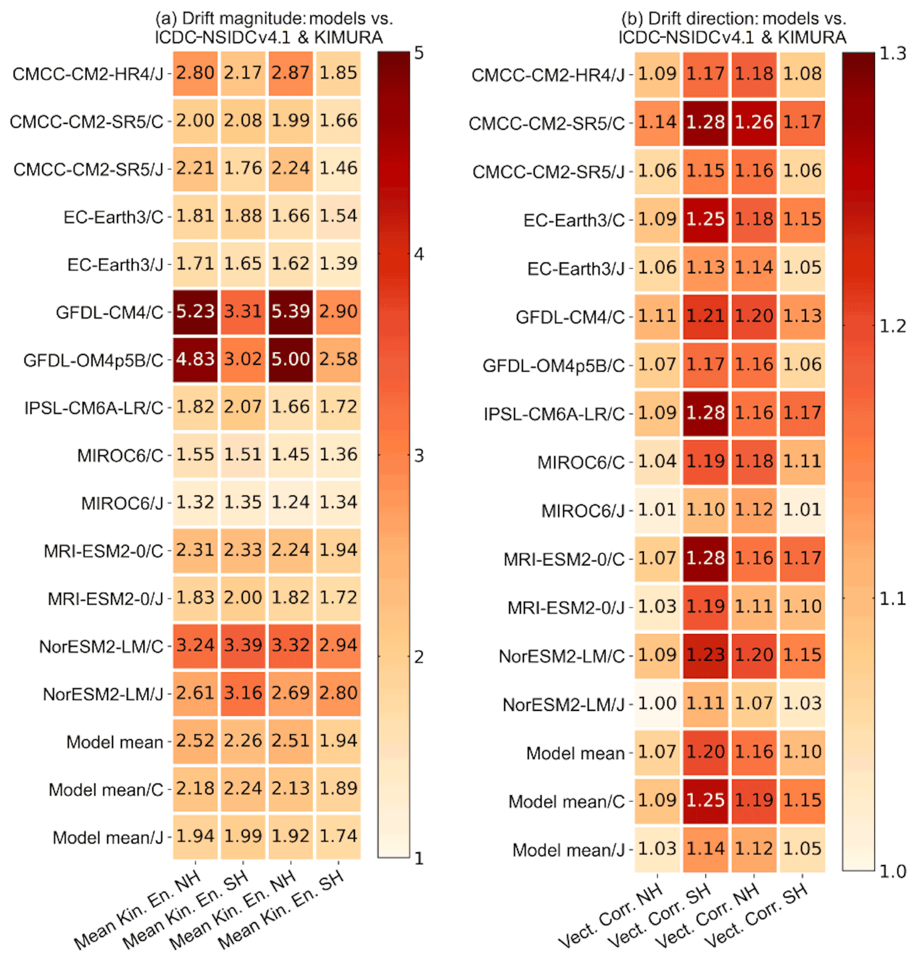
Figure 10 The ice drift metrics of 14 model outputs under OMIP1 (/C) and OMIP2 (/J) protocols, 14-model mean (model mean), five-OMIP1-model mean (model mean/C) and five-OMIP2-model mean (model mean/J) from CMCC-CM2-SR5, EC-Earth3, MIROC6, MRI-ESM2-0, and NorESM2-LM. The four columns correspond to model performance metrics on the (a) MKE and (b) the vector correlations during 2003–2007 of the Arctic and Antarctic compared to the ICDC-NSIDCv4.1 (first two) and KIMURA data (last two). Lower values indicate better skill.

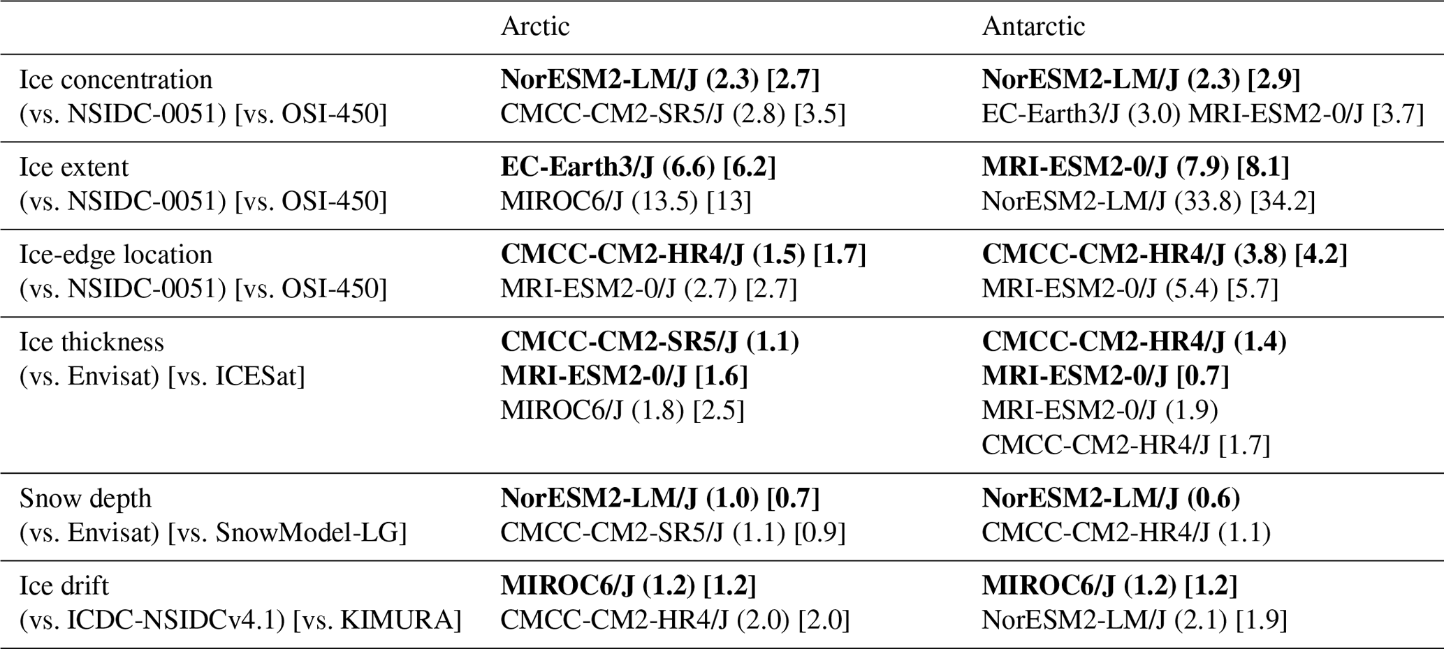
Table 4 The best- (in bold) and worst-performing models for the six evaluated sea ice variables, among the models forced by the JRA55-do reanalysis (CMCC-CM2-HR4, CMCC-CM2-SR5, EC-Earth3, MIROC6, MRI-ESM2-0, and NorESM2-LM). The numbers are derived from the performance metrics in Figs. 2, 5, 7, and 10 (marked as () and []). The values given average the three metrics (mean state, interannual variability, and trend) for ice concentration and ice extent from Figs. 2, 5a and b; the two metrics for the magnitude and vector correlations for ice drift from Fig. 10. The values for the ice-edge location, thickness, and snow depth are the metric of mean state from Figs. 5c and 7. In some cases, such as for the ice thickness evaluation, the best- and worst-performing models are different compared to different sets of observations.

3.4 Cross-metric analysis

From previous analyses, it seems that there is no best sea ice model simulation, but rather that each model has strengths and weaknesses. To further illustrate this aspect, the metrics of each sea ice variable are ranked in a cross-metric analysis, where the link between the model performance in one variable and the performance in another is clearly highlighted. By changing the atmospheric forcing from CORE-II to JRA55-do reanalysis data, the sea ice model simulations are improved in general. In order to make the comparison simple, six models (CMCC-CM2-HR4, CMCC-CM2-SR5, EC-Earth3, MIROC6, MRI-ESM2-0, and NorESM2-LM) forced by the JRA55-do reanalysis were retained for this analysis. The best- and worst-performing models for six ice variables are listed in Table 4. It is found that no single model performs best in all ice metrics, as there is no link between performance in one variable and performance in another. For example, the NorESM2-LM/J is the best regarding the ice concentration and snow depth simulation, but the worst for the ice drift simulation in the Antarctic, and MIROC6/J is the best regarding the ice drift simulation but the worst for the ice extent and thickness simulation in the Arctic.

4 Conclusions and discussion

SITool (v1.0), a performance metrics and diagnostics tool for CMIP6-compliant sea ice outputs, is introduced in this paper. The evaluation includes ice concentration, extent, edge location, thickness, snow depth, and ice drift. SITool (v1.0) provides rating scores for each sea ice variable in both hemispheres by comparing them to a set of observational references, using two observational references to account for the role of observational uncertainty in the evaluation process. In this paper, we evaluate the CMIP6 OMIP sea ice simulations with SITool (v1.0) to demonstrate the proof of concept and potentialities behind it. Specifically, we evaluate the performance of OMIP historical sea ice simulations (1980–2007 for sea ice areal properties, 2003–2007 for ice drift, thickness, and snow depth).

Our main findings on CMIP6 OMIP simulations are summarized below. By changing the atmospheric forcing from CORE-II to JRA55-do reanalysis data, improvements are identified in (1) the ice concentration simulations including the mean, interannual variability, and trend in both hemispheres, (2) the ice extent simulations including the mean and interannual variability in the Arctic, as well as the interannual variability and trend in the Antarctic, (3) the mean ice-edge location simulations in both hemispheres, (4) the mean ice thickness simulations in the Antarctic and the mean snow depth simulations in both hemispheres, and (5) the ice drift simulations including the magnitude and direction in both hemispheres. By increasing the horizontal resolution of the CMCC-CM2 ocean–sea ice model, the improvements are identified in the sea ice concentration (mean, interannual variability, and trend) and the mean ice-edge location simulations in both hemispheres.

In general, model errors are larger than observational uncertainty, and model performance on the ice concentration, extent, edge location, and ice drift simulations is consistent when comparing to different observational references. For the ice thickness and snow depth evaluation, the rating scores are not consistent compared to different observational references, which is due to the limited observations and to the fact that different months were chosen for comparison during 2003–2007. This finding shows that sea ice thickness and snow depth estimates are still at an earlier stage of maturity compared to datasets of sea ice concentration or drift.

The improvements of mean ice concentration simulations in the summer for both hemispheres by changing the atmospheric forcing and increasing the horizontal resolution are also identified in Tsujino et al. (2020) and Chassignet et al. (2020). The reduced mean ice extent bias in boreal summer and much improved interannual variability of ice extent in OMIP2 simulations are also proved in Tsujino et al. (2020). For the mean ice thickness simulation, Chassignet et al. (2020) also shows that the improvement is not obvious by increasing the horizontal resolution of ocean–sea ice models. To understand the processes leading to the improvement of model simulations under different atmospheric forcings and ocean–sea ice models, we will discuss the sensitivity of sea ice simulation to CMIP6 OMIP model physics in an upcoming companion paper.

The metrics make a summary of the model performance on different aspects of the sea ice system to help detect the inter-model differences or track the time evolution of model performance efficiently. However, the usage of metrics comes at the risk of over-interpretation by summarizing all the complex behavior of models to one number. In fact, a good metric can be obtained for many wrong reasons, so we do not recommend relying exclusively on these metrics to orient strategic choices regarding, e.g., sea ice model development. While it is running, SITool (v1.0) produces spatial maps (Figs. 8, 9 and Figs. A1–A12 in Appendix A) and time series diagrams (Figs. 3, 4, 6) that can be consulted by the expert to understand the origin of one particular metric value.

While SITool (v1.0) is primarily designed to assess ocean–sea ice simulations forced by atmospheric reanalysis, it can also be used to evaluate coupled model simulations (e.g., CMIP6 historical runs). We draw the reader's attention to the fact that, in that case, several metrics may become less relevant and less easy to interpret. Indeed, a coupled model is not supposed to produce sea ice output that is in phase with real observations due to the presence of irreducible climate internal variability. This is particularly true for the evaluation of sea ice thickness and snow depth, for which the limited time span (2003–2007) is likely not enough to draw robust conclusions regarding model performance.

Appendix A: Sea ice diagnostics

In this appendix, additional sea ice diagnostics are given to help understand why metrics vary from one dataset to the next. The spatial distribution of the differences between model simulations and the observational reference is presented in Figs. A1–A12 and the model simulations under OMIP1 and OMIP2 protocols are listed in the second and third columns, respectively. This includes the 1980–2007 September and February mean ice concentration differences (Figs. A1–A4), the 2003–2007 winter-mean ice thickness (Figs. A5–A6) and snow depth differences (Figs. A7–A8) (February for the Arctic and September for the Antarctic), and the 2003–2007 September and February mean ice-motion MKE differences (Figs. A9–A12).

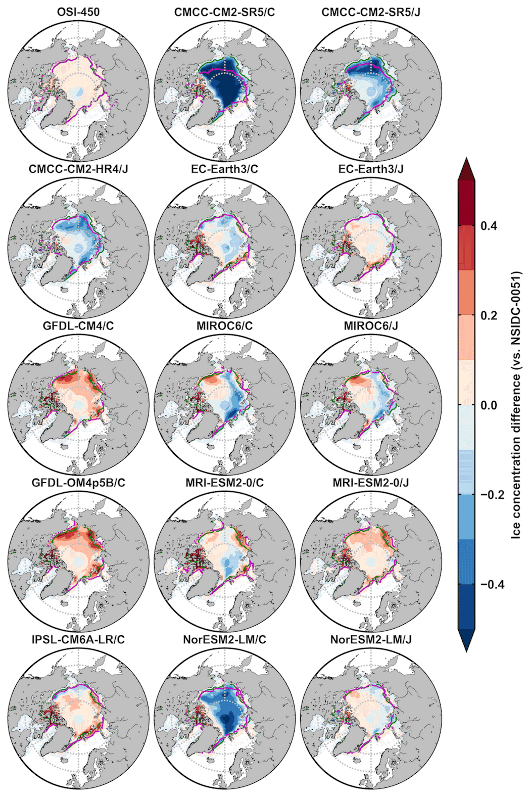
Figure A1 The 1980–2007 September mean Arctic ice concentration differences between OSI-450/model outputs and the NSIDC-0051 data (colors), and contours of 15 % concentration of the NSIDC-0051 data (green lines) and OSI-450/model outputs (magenta lines). The second and third columns are from the five OMIP1 and OMIP2 model outputs of CMCC-CM2-SR5, EC-Earth3, MIROC6, MRI-ESM2-0, and NorESM2-LM, respectively.

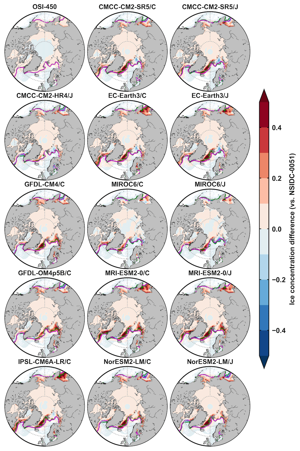
Figure A2 The 1980–2007 February mean Arctic ice concentration differences between OSI-450/model outputs and the NSIDC-0051 data (colors), and contours of 15 % concentration of the NSIDC-0051 data (green lines) and OSI-450/model outputs (magenta lines). The second and third columns are from the five OMIP1 and OMIP2 model outputs of CMCC-CM2-SR5, EC-Earth3, MIROC6, MRI-ESM2-0, and NorESM2-LM, respectively.

Figure A3 The 1980–2007 February mean Antarctic ice concentration differences between OSI-450/model outputs and the NSIDC-0051 data (colors), and contours of 15 % concentration of the NSIDC-0051 data (green lines) and OSI-450/model outputs (magenta lines). The second and third columns are from the five OMIP1 and OMIP2 model outputs of CMCC-CM2-SR5, EC-Earth3, MIROC6, MRI-ESM2-0, and NorESM2-LM, respectively.

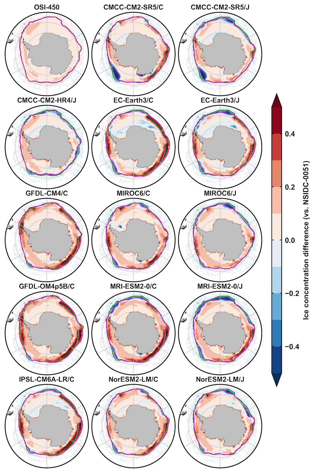
Figure A4 The 1980–2007 September mean Antarctic ice concentration differences between OSI-450/model outputs and the NSIDC-0051 data (colors), and contours of 15 % concentration of the NSIDC-0051 data (green lines) and OSI-450/model outputs (magenta lines). The second and third columns are from the five OMIP1 and OMIP2 model outputs of CMCC-CM2-SR5, EC-Earth3, MIROC6, MRI-ESM2-0, and NorESM2-LM, respectively.

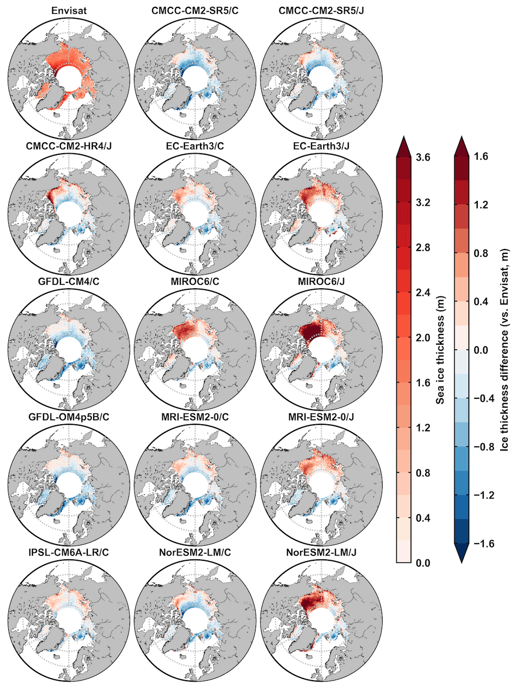
Figure A5 The 2003–2007 February mean Arctic ice thickness from Envisat data (first picture, m) and ice thickness differences between model outputs and Envisat data (m). The second and third columns are from the five OMIP1 and OMIP2 model outputs of CMCC-CM2-SR5, EC-Earth3, MIROC6, MRI-ESM2-0, and NorESM2-LM, respectively.

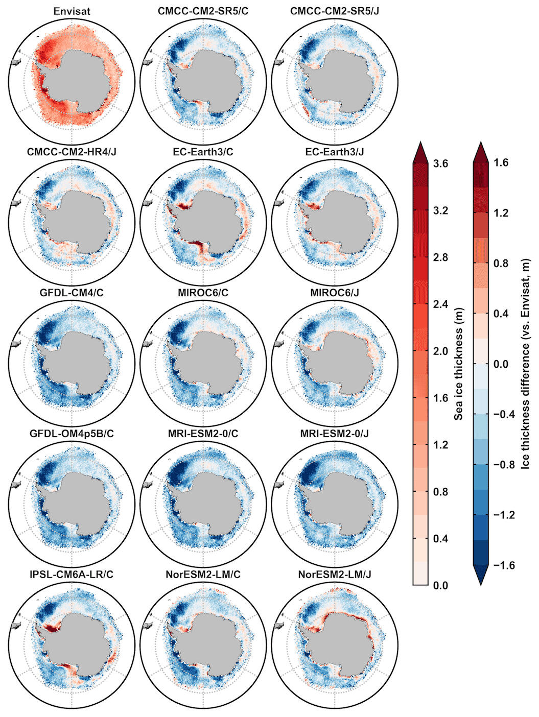
Figure A6 The 2003–2007 September mean Antarctic ice thickness from Envisat data (first picture, m) and ice thickness differences between model outputs and Envisat data (m). The second and third columns are from the five OMIP1 and OMIP2 model outputs of CMCC-CM2-SR5, EC-Earth3, MIROC6, MRI-ESM2-0, and NorESM2-LM, respectively.

Figure A7 The 2003–2007 February mean Arctic snow depth from Envisat data (first picture, m) and snow depth differences between model outputs and Envisat data (m). The second and third columns are from the five OMIP1 and OMIP2 model outputs of CMCC-CM2-SR5, EC-Earth3, MIROC6, MRI-ESM2-0, and NorESM2-LM, respectively.

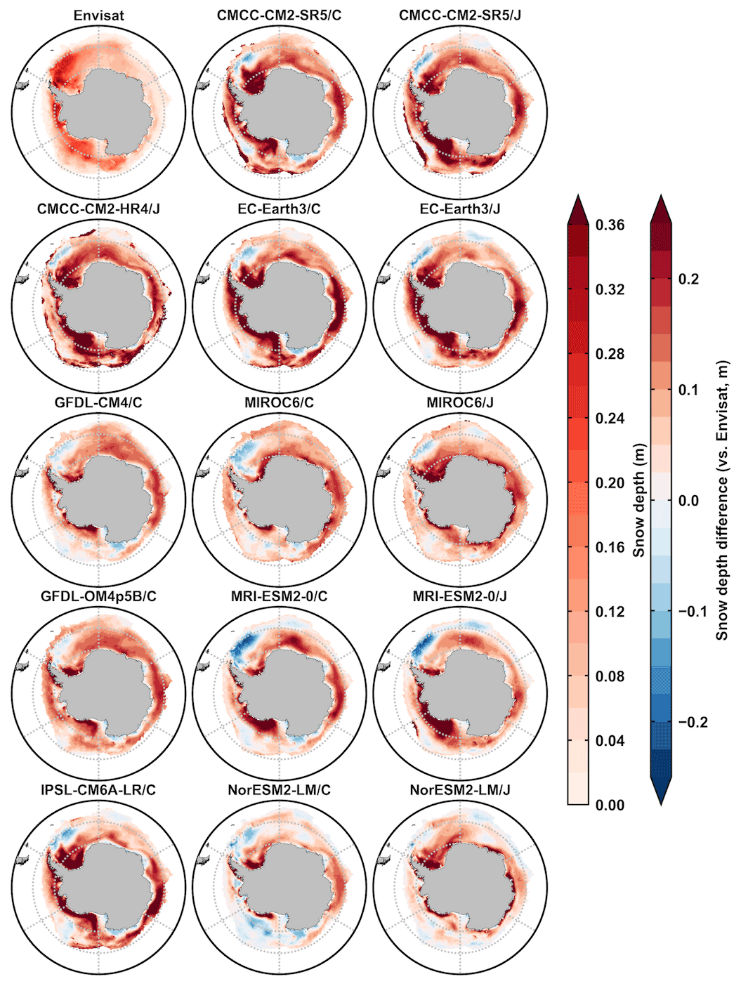
Figure A8 The 2003–2007 September mean Antarctic snow depth from Envisat data (first picture, m) and snow depth differences between model outputs and Envisat data (m). The second and third columns are from the five OMIP1 and OMIP2 model outputs of CMCC-CM2-SR5, EC-Earth3, MIROC6, MRI-ESM2-0, and NorESM2-LM, respectively.

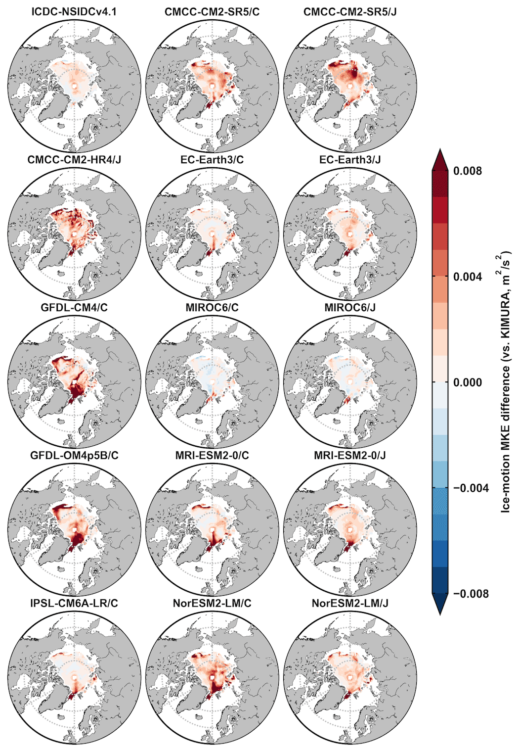
Figure A9 The 2003–2007 September mean Arctic ice-motion MKE differences between ICDC-NSIDCv4.1/model outputs and the KIMURA data (m² s⁻²). The second and third columns are from the five OMIP1 and OMIP2 model outputs of CMCC-CM2-SR5, EC-Earth3, MIROC6, MRI-ESM2-0, and NorESM2-LM, respectively.

Figure A10 The 2003–2007 February mean Arctic ice-motion MKE differences between ICDC-NSIDCv4.1/model outputs and the KIMURA data (m² s⁻²). The second and third columns are from the five OMIP1 and OMIP2 model outputs of CMCC-CM2-SR5, EC-Earth3, MIROC6, MRI-ESM2-0, and NorESM2-LM, respectively.

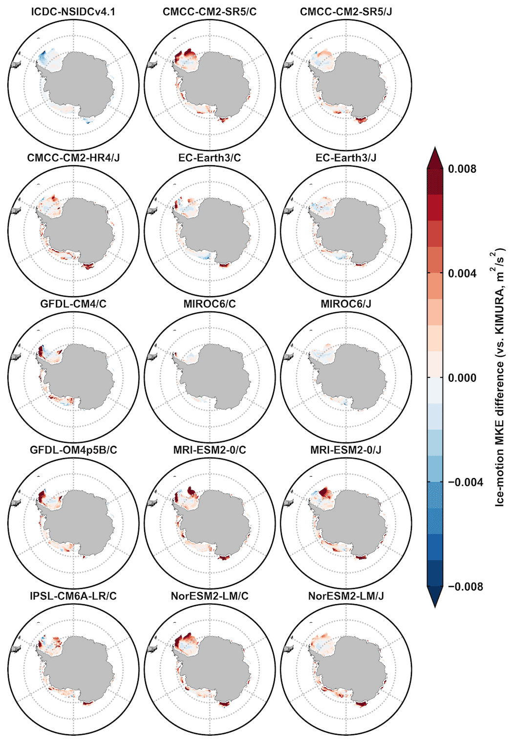
Figure A11 The 2003–2007 February mean Antarctic MKE differences between ICDC-NSIDCv4.1/model outputs and the KIMURA data (m² s⁻²). The second and third columns are from the five OMIP1 and OMIP2 model outputs of CMCC-CM2-SR5, EC-Earth3, MIROC6, MRI-ESM2-0, and NorESM2-LM, respectively.

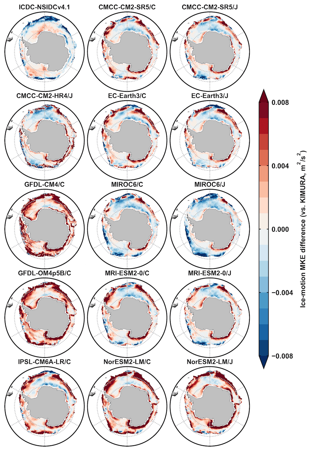
Figure A12 The 2003–2007 September mean Antarctic MKE differences between ICDC-NSIDCv4.1/model outputs and the KIMURA data (m² s⁻²). The second and third columns are from the five OMIP1 and OMIP2 model outputs of CMCC-CM2-SR5, EC-Earth3, MIROC6, MRI-ESM2-0, and NorESM2-LM, respectively.