Impact of Infrared Atmospheric Sounding Interferometer (IASI) thermal infrared measurements on global ozone reanalyses

The information content of thermal infrared measurements for tropospheric ozone (O₃) estimation has already been well demonstrated. However, the impact of such measurements to constrain modelled O₃ distributions within global assimilation systems is not yet unequivocal. A new tropospheric O₃ reanalysis is computed for the year 2010 by means of assimilating measurements from the Infrared Atmospheric Sounding Interferometer (IASI) within the MOdéle pour la Chimie Á Grande Echelle (MOCAGE) chemical transport model. The objective is to evaluate the impact of recent methodological improvements of the data assimilation scheme on the O₃ distribution. The new O₃ reanalysis (named IASI-r) and its precursor (IASI-a) have been validated against ozonesondes, and compared to independent estimations of tropospheric O₃ and to results from two state-of-the-art products based on detailed tropospheric chemistry (the Goddard Earth Observing System with a coupled chemistry–climate model, GEOS-CCM, and the Copernicus Atmosphere Monitoring Service, CAMS, reanalysis). The main difference between IASI-r and IASI-a concerns the treatment of IASI observations, with radiances being assimilated directly in IASI-r instead of intermediate Level 2 O₃ retrievals. IASI-r is found to correct major issues with IASI-a, such as the neutral or negative impact of IASI assimilation in the extra-tropics and the presence of residual biases in the tropics. IASI-r also compares relatively well to the CAMS reanalysis, which is based on a more comprehensive chemical mechanism and the assimilation of several ultraviolet (UV) and microwave measurements.

1 Introduction

Tropospheric ozone (O₃) contributes to global warming with a net positive effect in the upper troposphere–lower stratosphere (UTLS) at tropical and subtropical latitudes (Stevenson et al., 2013). Tropospheric O₃ evolution is driven by both natural and anthropogenic processes, such as photochemical production from primary pollutants, convection, long-range transport, and stratosphere–troposphere exchanges (Young et al., 2013). Furthermore, natural atmospheric oscillations like the El Niño–Southern Oscillation (ENSO) can contribute significantly to the variability in the O₃ concentration in the tropical UTLS (Ziemke et al., 2015).

The complexity of O₃ processes (sources, sinks, and transport patterns) and the scarcity of direct O₃ measurements in the UTLS (Cooper et al., 2014) make the use of atmospheric composition models necessary for the estimation of the O₃ radiative forcing (Gauss et al., 2006). Recent model intercomparison exercises such as the Atmospheric Chemistry and Climate Model Intercomparison Project (ACCMIP; Lamarque et al., 2013) estimated the present-day O₃ radiative forcing uncertainty to be 30 % (Stevenson et al., 2013), due to uncertainties in O₃ modelling.

Satellite measurements provide global and independent estimates of O₃, although with limited vertical information. An estimation of tropospheric O₃ columns can be obtained by combining stratospheric profiles from microwave limb sounders with total O₃ columns from ultraviolet (UV) nadir sounders. For example, Ziemke et al. (2006) combined retrievals from the Ozone Monitoring Instrument (OMI) and from the Microwave Limb Sounder (MLS) on board the Aura satellite to provide a tropospheric ozone column (TOC) product, which will hereafter be called “OMI-MLS”. Thermal sounders like the Tropospheric Emission Spectrometer (TES; Bowman et al., 2006) or the Infrared Atmospheric Sounding Interferometer (IASI; Clerbaux et al., 2009; Hilton et al., 2012) add complementary information to UV and limb sounders due to a peak of sensitivity in the UTLS region within the 10 µm spectral region. Another advantage of thermal sounders is the possibility to retrieve O₃ during night-time, thereby providing observations during the polar nights. Recently, there have been growing efforts to comparatively evaluate tropospheric O₃ retrievals from UV and IR measurements (Gaudel et al., 2018) in the perspective of present O₃ variability and trends. These studies have highlighted some inconsistencies between UV and infrared (IR) retrievals, in terms of O₃ columns and observed trends, that are currently being addressed.

Satellite measurements are also assimilated routinely in global chemistry models (Bocquet et al., 2015) to either improve chemical forecasts (Flemming et al., 2015) or to produce more accurate reanalyses of the past atmospheric composition (Inness et al., 2019). However, due to the difficulties involved in harmonizing more recent IR products with well-established UV products, chemical assimilation systems still rely mostly on UV or limb O₃ measurements (Van Peet et al., 2018; Inness et al., 2019). Because of the weak sensitivity of UV measurements to the troposphere, tropospheric O₃ is thus constrained indirectly through the simultaneous fit to total and stratospheric columns. An exception is represented by the reanalysis of Miyazaki et al. (2015), which assimilated tropospheric TES O₃ profiles. However, the reduced availability of TES data after 2010 impeded the production of an O₃ reanalysis constrained by IR measurements for the entire period. Huijnen et al. (2020) compared the accuracy of the tropospheric O₃ reanalyses of Inness et al. (2019) and Miyazaki et al. (2015) against radio soundings and found similar accuracies for both. The IASI mission provides uninterrupted measurements from 2008, with three sensors flying today (Metop A, B, and C) and plans for long-term continuation of operations in the next decade (IASI-NG). Although IASI O₃ observations might be very valuable for long reanalyses, they have not yet been assimilated within any of the currently available chemical reanalysis.

Global assimilation of IASI O₃ products have been examined in a number of previous studies. Massart et al. (2009) were the first to assimilate IASI total O₃ columns in a chemical transport model (CTM), and the authors highlighted the need to employ averaging kernels to correctly weight the instrument sensitivity. Emili et al. (2014) examined the assimilation of tropospheric columns (240–1000 hPa) using retrievals kernels and found a positive impact at tropical latitudes but a slightly negative impact at mid-latitudes and high latitudes. Peiro et al. (2018) used the same methodology as Emili et al. (2014) to compute tropospheric O₃ analyses in the tropics to study the O₃ ENSO signal. All of these studies performed a bias correction prior to the assimilation of retrieved quantities (also named Level 2 or L2 products) to avoid increased biases in the O₃ reanalyses. The empirical nature of the bias correction procedure could not ensure a positive (or neutral) impact of IR assimilation at all latitudes and vertical levels. More recently, Emili et al. (2019) evaluated the direct assimilation of Level 1 (L1) radiances from IASI to overcome some of the previous difficulties encountered and found that more variability can be extracted from IASI spectra when directly assimilating the radiances. Barret et al. (2020) confirmed that the use of a dynamical a priori based on the tropopause height significantly improved O₃ retrievals at southern mid-latitudes. Finally El Aabaribaoune et al. (2021) improved the L1 assimilation scheme by employing a more realistic observation error covariance for the L1 radiances, which reduced residual stratospheric biases. However, both the analyses of Emili et al. (2019) and El Aabaribaoune et al. (2021) were limited to a single summer month in 2010 and could not draw conclusions on the capacity of IR assimilation to reproduce the seasonal O₃ variability or trends in the extra-tropics. Note that the assimilation of IASI radiances sensitive to O₃ was also investigated in the framework of numerical weather prediction (NWP) by Dragani and Mcnally (2013) and, more recently, Coopmann et al. (2018). O₃ information from IR sounders could in fact improve NWP through the tracer effect (Dragani and Mcnally, 2013) or due to increased temperature and humidity information content (Coopmann et al., 2020). However, some difficulties still persist with respect to the correction of biases and the appearance of drifts related to the variational bias correction (Dragani and Mcnally, 2013). To conclude, there is a strong need to further assess the benefits of IASI IR observations for UTLS O₃ analyses both for chemical and meteorological applications.

The objective of this paper is to evaluate a new O₃ reanalysis during a full year (2010), based on the assimilation of IASI measurements within the MOdéle pour la Chimie Á Grande Echelle (MOCAGE) CTM (Josse et al., 2004). This new reanalysis profits from all methodological improvements achieved in the recent years concerning IASI O₃ assimilation. In particular, the major difference with the multi-year O₃ reanalysis of Peiro et al. (2018) (hereafter called IASI-a) is that the IASI L1 spectrum is now assimilated directly and without performing any empirical bias correction. In this study, we keep the simpler description of O₃ based on linearized chemistry (Cariolle and Teyssedre, 2007) already used in previous global reanalyses (Massart et al., 2009; Emili et al., 2014; Peiro et al., 2018) to assess the improvements in the assimilation scheme alone. On top of the usual validation against ozonesonde measurements, the obtained O₃ fields will be compared to IASI-a, to output from a chemistry–climate model used in ACCMIP (the Goddard Earth Observing System model with a coupled chemistry–climate module, GEOS-CCM), and to the Copernicus Atmosphere Monitoring Service (CAMS) atmospheric composition reanalysis (CAMSRA; Inness et al., 2019). Thus, we will verify the added value of IR assimilation to map the O₃ 3D distribution with respect to existent state-of-the-art techniques based either on full-chemistry modelling or a combination of modelling and satellite data assimilation (non IR). Results with the tested configuration might also be of interest for NWP models, which are generally based on O₃ linearized schemes (Han and McNally, 2010) for reasons of computational efficiency. Hence, in the context of ongoing efforts to include more detailed chemical modelling within NWP, this study can provide further insights into the trade-off between adding more complexity to the model and better exploiting current and future satellite measurements.

The paper is structured as follows. Section 2 summarizes the O₃ modelling and reanalysis datasets that were already publicly available prior to this work and that are used here for comparison. The measurements that are assimilated to produce the new reanalysis and those that are used for independent validation are detailed in Sect. 3. The configuration of the chemistry transport model and the set-up of the assimilation experiment are described in Sect. 4. The results section (Sect. 5) is split into four subsections: the first subsection (Sect. 5.1) is focused on the validation of the new reanalysis against ozonesondes, specifically with respect to IASI-a; the second, third, and fourth subsections (Sects. 5.2, 5.3, and 5.4 respectively) provide some further comparisons with tropospheric O₃ retrievals and the modelling and assimilation datasets of ACCMIP and CAMSRA. Conclusions and perspectives of this work are summarized in the last section.

2 Previous modelling and assimilation experiments

2.1 GEOS-CCM

The Goddard Earth Observing System (GEOS) version 5.0 is a general circulation model developed by the National Aeronautics and Space Administration (NASA) that includes an interactive chemistry module for coupled chemistry–climate modelling (CCM). It is one of the models with detailed stratospheric and tropospheric chemistry schemes that took part in the ACCMIP exercise (Lamarque et al., 2013) and was used to estimate present and future O₃ radiative forcing (Stevenson et al., 2013). It also has one of the lowest tropospheric O₃ bias amongst the ACCMIP historical simulations (Young et al., 2013), and Oman et al. (2011) showed that it skilfully reproduces the tropospheric O₃ variability linked to ENSO. In the context of this study, we consider GEOS-CCM as representing state-of-the-art chemistry–climate simulations (without data assimilation). We downloaded monthly O₃ fields for 2010 from the historical climate ACCMIP simulation that is publicly available on the Centre for Environmental Data Analysis (CEDA) archive (http://archive.ceda.ac.uk, last access: 15 June 2020). Details on the set-up used for this simulation can be found in Lamarque et al. (2013).

2.2 CAMSRA

The chemical reanalysis provided by the Copernicus Atmosphere Monitoring Service (CAMS) is based on the Integrated Forecast System (IFS) general circulation model developed at ECMWF, which integrates detailed tropospheric chemistry and aerosol schemes (Flemming et al., 2015). Within IFS, the NWP data assimilation scheme was extended to assimilate satellite measurements of trace gases and aerosols. In the latest version of the CAMS reanalysis of the atmospheric composition (CAMSRA; Inness et al., 2019), measurements of O₃, CO, NO₂, and aerosol optical depth (AOD) are assimilated from a variety of satellites. Concerning O₃, no tropospheric measurements are currently assimilated in CAMSRA. Thus, tropospheric O₃ is constrained indirectly, either through the combination of total and stratospheric O₃ observations or through the assimilation of its chemical precursors (e.g. NO₂). Extensive validation (Inness et al., 2019; Huijnen et al., 2020) showed that biases of the CAMSRA O₃ reanalysis with respect to ozonesondes are generally lower than 10 % in the troposphere, compared with values of about 15 % for the ACCMIP free model simulations. Hence, CAMSRA represents a state-of-the-art O₃ reanalysis based on both comprehensive chemical modelling and most available satellite observations (except for IR sounders). CAMSRA monthly O₃ fields were downloaded from the CAMS data store (https://ads.atmosphere.copernicus.eu, last access: 16 June 2020).

2.3 IASI-a

The IASI-a global O₃ reanalysis (Peiro et al., 2018) is the outcome of several projects focused on the exploitation of satellite data for atmospheric analyses, which began with the Assimilation of Envisat Data (ASSET) project (Lahoz et al., 2007; Geer et al., 2006). In recent years, particular effort has been dedicated to hyperspectral IR measurements from IASI, which provide a wealth of information for tropospheric chemistry but are not yet assimilated in most operational centres. The IASI-a O₃ analysis discussed by Peiro et al. (2018) is based on a linearized O₃ chemistry configuration of the MOdéle pour la Chimie Á Grande Echelle (MOCAGE; Josse et al., 2004; Cariolle and Teyssedre, 2007) and on the joint assimilation of IASI tropospheric columns and stratospheric profiles from the Microwave Limb Sounder (Emili et al., 2014). SOftware for a Fast Retrieval of IASI Data (SOFRID) O₃ retrievals (Barret et al., 2011), which are based on a variational retrieval scheme and the RTTOV v9 radiative transfer model (Matricardi, 2009), have been assimilated within IASI-a. The biases of the IASI-a analysis are found to be smaller than 15 % in the tropical free troposphere (Peiro et al., 2018), suggesting that dense and frequent satellite observations such as IASI observations can partially make up for missing tropospheric chemistry in the model. However, no added value of IASI assimilation was found in the extra-tropics, and a degradation was even observed in the Southern Hemisphere (SH) mid-latitudes (Emili et al., 2014). Nevertheless, the IASI-a reanalysis represents a reference to evaluate potential improvements with respect to the assimilation of IASI measurements.

3 Measurements

In this study, we assimilate infrared spectra from the IASI sensor on board the Metop-A satellite (Clerbaux et al., 2009) and stratospheric O₃ profiles retrieved from MLS limb measurements (Froidevaux et al., 2008).

IASI spectral measurements (L1c data) contain calibrated and geolocalized spectra at 0.5 cm⁻¹ spectral resolution, i.e. 8461 radiance values for each ground pixel and a footprint of 12 km. Historical L1c data granules have been downloaded from the European Organisation for the Exploitation of Meteorological Satellites (EUMETSAT) Earth Observation data portal (https://eoportal.eumetsat.int, last access: 17 June 2020) in NETCDF (network Common Data Form) format. Data files contain also co-located land mask and cloud fraction values, obtained from Advanced Very High Resolution Radiometer (AVHRR) measurements, also on board Metop. As the AVHRR cloud mask is not available before 20 May 2010 we also downloaded the IASI L2 cloud products provided by EUMETSAT, which are based on a combination of multiple cloud detection algorithms (EUMETSAT, 2017).

The MLS V4.2 product (Livesey et al., 2020) contains retrieved O₃ profiles on 55 pressure levels ranging from 316 to 0.001 hPa with corresponding retrieval errors. Data have been downloaded from the Goddard Earth Sciences Data and Information Services Center (GES DISC) web portal (https://disc.gsfc.nasa.gov, last access: 17 June 2020). For a more detailed discussion on the accuracy of MLS retrievals for O₃ analyses, the reader is referred to Emili et al. (2019) or Errera et al. (2019).

Ozonesonde profiles and tropospheric columns derived from OMI-MLS observations (Ziemke et al., 2006) are used to compare the O₃ simulations to independent measurements. OMI-MLS tropospheric O₃ columns have already been used in the past to evaluate the tropical O₃ variability and have been compared to atmospheric chemistry models (Young et al., 2018; Ziemke et al., 2019). Ozonesonde data have been downloaded from the World Ozone and Ultraviolet Radiation Data Centre (WOUDC; http://www.woudc.org, last access: 17 June 2020), and OMI-MLS tropospheric O₃ have been downloaded from the GODDARD tropospheric ozone archive (https://acd-ext.gsfc.nasa.gov, last access: 18 June 2020). To compute model tropospheric O₃ columns that are coherent with the OMI-MLS estimation, we used the National Centers for Environmental Prediction (NCEP) tropopause monthly climatology, also available from the GODDARD archive.

4 Method

The new O₃ reanalysis (hereafter called IASI-r) fundamentally inherits the methodology from IASI-a (Emili et al., 2014; Peiro et al., 2018) but also includes the recent developments discussed by Emili et al. (2019) and El Aabaribaoune et al. (2021) concerning the direct assimilation of IASI L1 radiances. Therefore, we detail the novelties/changes introduced for this study and address the reader to the previous studies for a more detailed description on the aspects of the methodology that did not change. The reanalysis set-up and the differences between IASI-a and IASI-r are also summarized in Table 1.

Table 1 Configuration of the IASI-r and IASI-a (Peiro et al., 2018) experiments. The dash symbol indicates that the configuration is the same.

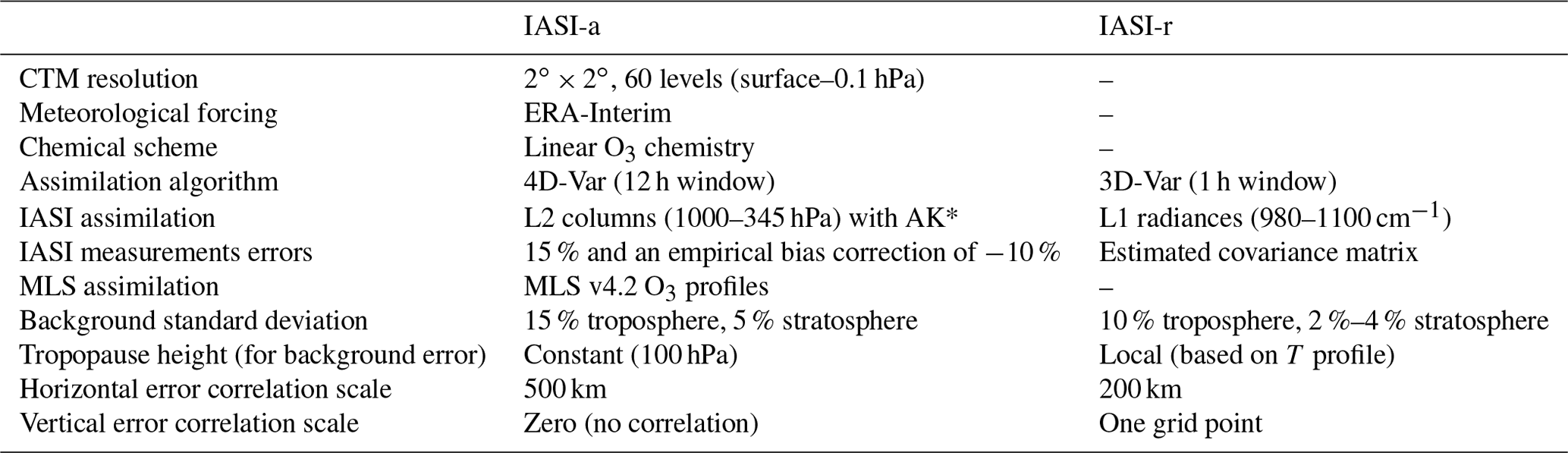
^∗ AK stands for averaging kernels.

4.1 Model and data assimilation scheme

The CTM MOCAGE is configured on a 2^∘ × 2^∘ global grid, with 60 vertical levels up to 0.1 hPa. It is forced by ERA-Interim meteorological fields (Dee et al., 2011) and employs a linearized O₃ chemistry scheme (Cariolle and Teyssedre, 2007). The CTM configuration is identical to the IASI-a reanalysis (Peiro et al., 2018). As discussed by Emili et al. (2014), the main limitation of this configuration is the missing tropospheric O₃ chemistry and the main advantage is the reduced computational cost. However, it represents a good choice to implement and evaluate the assimilation of new satellite retrievals. Indeed, a similar set-up has been used to compute the 4-year-long O₃ reanalysis of Van Peet et al. (2018).

The employed assimilation algorithm is an hourly 3D-Var, as in Emili et al. (2019), which differs from the 4D-Var used by Peiro et al. (2018) and Emili et al. (2014). Due to recent optimizations of the MOCAGE code, the former implementation of the linearized and adjoint CTM codes are not yet available within the latest versions of the assimilation suite, which determined the switch to 3D-Var. However, assimilation experiments conducted with MLS observations revealed that O₃ differences between a 3D-Var and 4D-Var algorithm are very small within the adopted model configuration (less than 1 % difference on global averages, not shown).

The assimilation of IASI L1c spectra is performed through the radiative transfer model (RTM) RTTOV V11.3 (Saunders et al., 2013). The treatment of surface emissivity, skin temperature, and all other variables related to the radiative transfer follows the method described in Emili et al. (2019). The assimilation of MLS O₃ profiles is performed as described either in Peiro et al. (2018) or Emili et al. (2019). To summarize, the CTM is kept identical to IASI-a, and the data assimilation is changed only in terms of the 4D-Var (IASI-a) versus 3D-Var (IASI-r), the treatment of IASI data (L1 radiances assimilated in IASI-r instead of L2 columns in IASI-a), and the version of the radiative transfer model used (RTTOV11 for radiance assimilation instead of RTTOV9 for the L2 retrievals' assimilation).

4.2 Observations

We assimilate only clear-sky IASI L1c radiances in the main O₃ window (980–1100 cm⁻¹) using the same channel selection as described in Emili et al. (2019). A slightly different clear-sky selection procedure than in Emili et al. (2019) has been employed here, as the availability of cloud retrievals from AVHRR and IASI is not homogeneous during 2010: the AVHRR cloud mask is not available before May 2010 in the EUMETSAT L1c data, and the EUMETSAT L2 cloud retrievals are flawed from September to December 2010. Therefore, we used the EUMETSAT L2 cloud mask until September 2010 and the AVHRR cloud mask afterward. In both cases, the same strict threshold of 1 % is imposed on the cloud fraction to reduce possible cloud contamination as much as possible (Emili et al., 2019). Pixels affected by a strong dust spectral signature are also filtered out (Emili et al., 2019) as well as those with a surface emissivity smaller than 0.95 (mostly deserts), to avoid potential issues with O₃ inversion. Data thinning is performed using a regular grid of 1^∘ × 1^∘ resolution and selecting the first pixel that falls in every two grid boxes. This ensures a minimum distance of 1^∘ among assimilated observations. Finally, a dynamical filter is used to reject pixels that differ from modelled radiances by more than 12 %. This is done to avoid assimilating observations that, for some undetected reason (e.g. erroneous surface properties or poor model representativity), differ significantly from their model counterparts. The value of the threshold is about twice the standard deviation of the observation minus background values and allows one to reject a relatively small number of potential outliers (< 5 %; see also Emili et al., 2019) that might have passed the previous filters. After the selection, the number of assimilated IASI observations varies between 6000 and about 8000 d⁻¹.

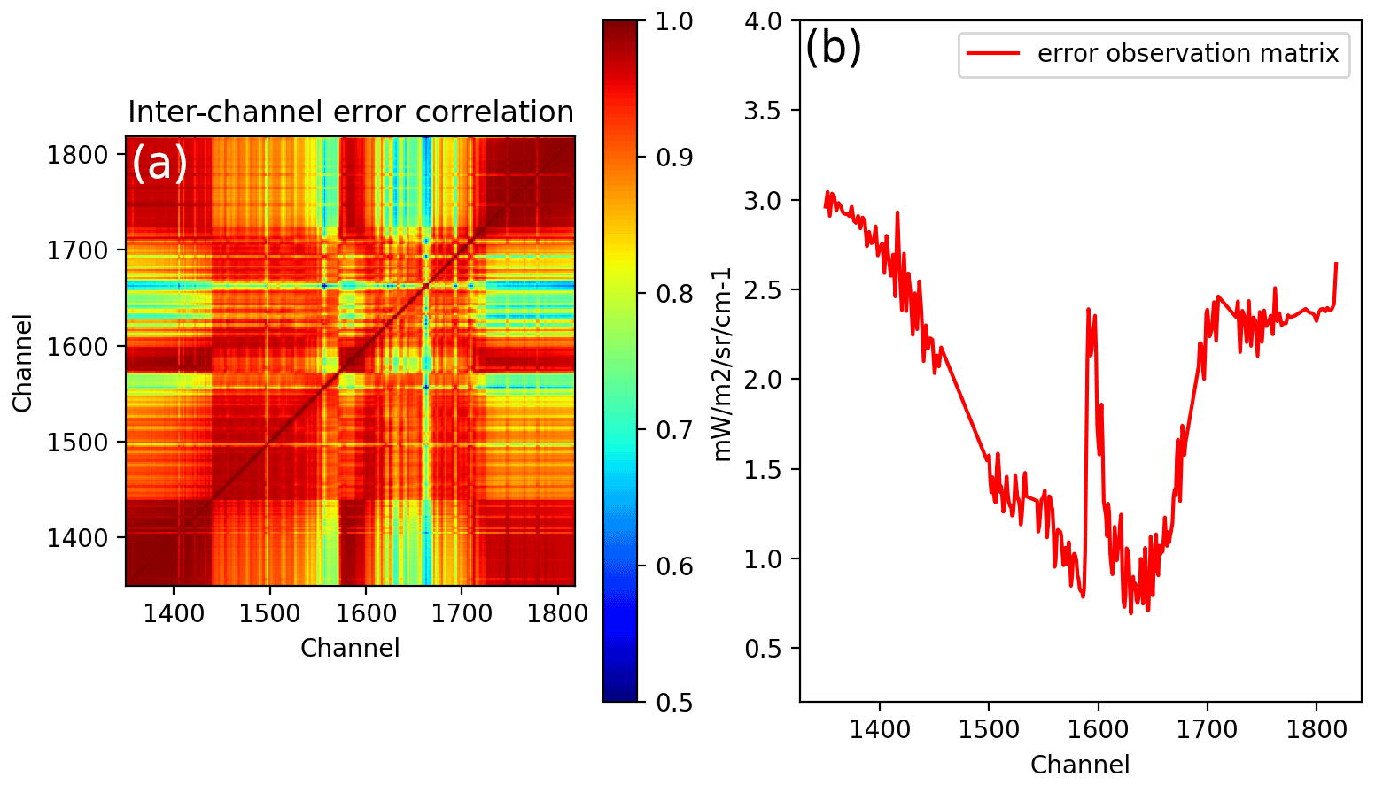
Figure 1 Observation error covariance used to assimilate IASI L1 radiances in this study: correlation matrix (a) and error standard deviation (squared diagonal of the covariance matrix, b). The x and y axes in panel (a) and the x axis in panel (b) report the IASI spectral channel's number within the 980–1100 cm⁻¹ window.

The single and most significant difference in the assimilation of IASI radiances with respect to Emili et al. (2019) is that we employed a diagnosed observation error covariance (R) instead of the prescribed and diagonal one used previously. This choice is motivated by the results of El Aabaribaoune et al. (2021), who found that a diagnosed R with non-zero inter-channel error correlations can reduce stratospheric biases otherwise introduced by IASI assimilation. The diagnostic of R is based on innovation statistics (Desroziers et al., 2005), and we followed the procedure suggested by El Aabaribaoune et al. (2021): (i) we first ran an assimilation experiment using the same R as in Emili et al. (2019) (diagonal with a standard deviation of 0.7 mW m⁻² sr⁻¹ cm), (ii) we diagnosed R on an average period of 1 month, (iii) we used the obtained R to run a second assimilation experiment for a longer period, (12 months) and we again estimated R. The latter R estimation is the one that is used to compute IASI-r because it provides slightly superior results with respect to the first estimation (not shown; see also the discussion in El Aabaribaoune et al., 2021). The employed R (Fig. 1) is found to be similar to the error covariance matrices estimated by El Aabaribaoune et al. (2021), i.e. it presents significant inter-channel error correlations and an error standard deviation matching the typical spectral signature of O₃ absorption in the IR.

Concerning the MLS, we assimilated only O₃ concentrations above 170 hPa and made use of retrieval errors to prescribe R (Emili et al., 2019).

4.3 Background error covariance

The background error covariance B has been slightly improved with respect to previous studies, which prescribed O₃ error profiles based on a single and fixed tropopause height (Emili et al., 2014; Peiro et al., 2018; Emili et al., 2019; El Aabaribaoune et al., 2021). For this study, the tropopause height is computed every 3 h based on the model temperature profiles (ERA-Interim) and using the 2 K m⁻¹ lapse rate definition of the World Meteorological Organization (WMO). The background error standard deviation is prescribed as a percentage of the background O₃ profile but with refined values depending on the layer (10 % in the troposphere, 1 % close to the tropopause, 4 % in the lower stratosphere, and 2 % in the upper stratosphere) and with a correct definition of the tropopause that depends now on the hour and the geographical position. The smaller errors in correspondence of the tropopause layer reduce the spread of large stratospheric increments into the troposphere. Horizontal and vertical error correlations have been kept the same as in Emili et al. (2019).

Using the new dynamical parameterization of the background standard deviation instead of the one described by Peiro et al. (2018) mostly provided a reduction in the bias of about 10 % around the tropopause (not shown).

5 Results

We examine O₃ simulations for the full year for 2010, which is characterized by a sharp transition from positive (El Niño) to negative (La Niña) ENSO conditions (Peiro et al., 2018). The corresponding large departure from climatological O₃ in the tropics represents an ideal condition for evaluating chemical simulations. Looking at a full year also allows for the evaluation of a complete O₃ seasonal cycle in the extra-tropics, which is missing in recent studies (Emili et al., 2019; El Aabaribaoune et al., 2021).

The IASI-r analysis was initialized with the output of a free MOCAGE simulation on 1 January 2010 and run until 31 December 2010, assimilating IASI and MLS observations. In parallel, a free model simulation without data assimilation was computed for the same period and named “Control”. Note that the control simulation is identical to the one already discussed in Peiro et al. (2018).

First, IASI-r is validated against ozonesondes and compared to IASI-a (Sect. 5.1) in order to quantify the improvements with respect to the previous reanalysis. A multi-model intercomparison is then presented (Sect. 5.2, 5.3, and 5.4) to evaluate IASI-r against existing state-of-the-art chemistry models, reanalyses, and OMI-MLS retrievals. All reported statistics represent either yearly or monthly data averages.

5.1 Validation against ozonesondes

Matches between IASI-r and ozonesondes profiles were computed online during the simulation, through a linear interpolation of hourly O₃ fields at the time and location of each ozonesonde measurement. Original ozonesonde profiles were interpolated to a coarser vertical grid, representative of MOCAGE vertical resolution prior to this matching. Thus, all pairs of matched profiles are defined over the same pressure grid (using missing values when necessary), which allows a straightforward computation of average statistics. The same strategy has been used to compute matches between ozonesondes and IASI-a, except for the temporal interpolation, which is done using 6-hourly model outputs instead of hourly ones, due to the limited availability of archived IASI-a data. The impact of the different temporal interpolation on the validation statistics has been found to be non-significant.

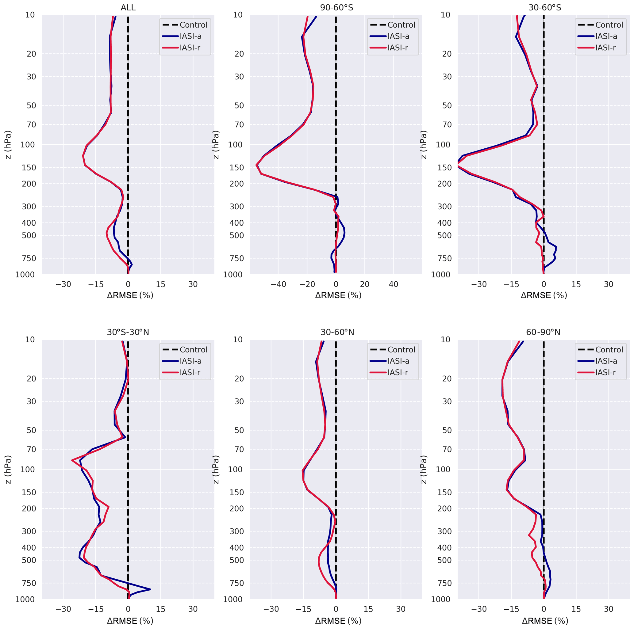
Figure 2 Relative gain in the root-mean-square error (RMSE) with respect to radio soundings averaged globally (top-left plot) and for five respective latitude bands: 90–60^∘ S, 30–60^∘ S, 30^∘ S–30^∘ N, 30–60^∘ N, and 60–90^∘ N (see panel headings). IASI-a is depicted in blue, and IASI-r is shown in red. Negative values indicate a decrease (improvement) in the RMSE with respect to the control simulation (dotted line), whereas positive values indicate an increase (degradation) in the RMSE with respect to the control simulation.

The gain in the root-mean-square error (RMSE) with respect to ozonesondes for the full year is depicted in Fig. 2 for IASI-r and IASI-a (as a percentage of the ozonesondes concentration). The gain is computed by means of subtracting the RMSE of IASI-r and IASI-a from that of the control simulation, as in Emili et al. (2019). Negative values in Fig. 2 mean that the O₃ RMSE is improved with respect to the control simulation, whereas positive values mean degradation. This type of statistical indicator is commonly used to highlight differences between data assimilation experiments. We remark that both IASI-r and IASI-a improve the global RMSE by 5 % to 20 % depending on the altitude. The two reanalyses show almost identical skill above 300 hPa due to the positive impact of MLS that is assimilated in both experiments. However, IASI-r shows slightly superior results in the free troposphere (350–800 hPa). Differences in the troposphere become more evident when the RMSE gain is computed for different latitude bands. A well-known problem that affected previous reanalyses done using IASI O₃ retrievals is the appearance of positive biases in the SH and at high latitudes (Emili et al., 2014), which is highlighted by the degradation in the RMSE of the IASI-a reanalysis. With IASI-r, such degradation is not present: the RMSE gain is neutral in the SH and becomes slightly positive in the Northern Hemisphere (NH). In the tropics, where IASI has the largest sensitivity to tropospheric O₃, both IASI-r and IASI-a show the largest improvements in the O₃ profile, with similar gains of about 20 %, except for a spike in RMSE degradation that still occurred within IASI-a at about 800 hPa.

Figure 3 Monthly variability in the ozone free-troposphere column (345–750 hPa) averaged globally (top row) and for five respective latitude bands: 90–60^∘ S, 30–60^∘ S, 30^∘ S–30^∘ N, 30–60^∘ N, and 60–90^∘ N (see panel headings). The left column of the figure shows the absolute values of the O₃ columns (in DU) for IASI-a (orange line), IASI-r (green line), the control simulation (blue line), and the corresponding ozonesonde columns (black line). The right column of the figure shows the relative differences between the simulated and corresponding ozonesonde columns (as a percentage of ozonesonde columns).

Pairs of ozonesondes and model instantaneous profiles are used to compute monthly averaged O₃ columns, in order to further focus on the tropospheric O₃ variability. Figure 3 reports free-troposphere (345–750 hPa) O₃ columns measured by ozonesondes and the corresponding reanalyses values. The altitude range has been chosen to better investigate differences that appeared in Fig. 2. The figure reports absolute O₃ columns (in Dobson units, DU) for ozonesondes, IASI-r, IASI-a, and the control simulation (left column) as well as the corresponding relative differences between the simulation and the ozonesondes (right column). We remark that the seasonal variability in the O₃ column in the extra-tropics is much better described by IASI-r than by IASI-a, which is also reflected in the global plot. In particular, the difference between IASI-r and ozonesonde columns mostly remains below 10 %, whereas it reached values of +30 % (−20 %) in the 30–60^∘ S (30–60^∘ N) latitude band with IASI-a, sometimes even exceeding the error of the control simulation. The correspondence between IASI-r and ozonesondes is even remarkably good in the Arctic Circle (60–90^∘ N). Both IASI-r and IASI-a fail to reproduce the seasonal cycle of tropospheric O₃ in the Antarctic region (60–90^∘ S), which was also absent in the control simulation. In the tropical band (30^∘ S–30^∘ N), IASI-r and IASI-a provide similar results, as already suggested from Fig. 2.

It is highly likely that the large improvements in the extra-tropics with respect to IASI-a are a consequence of the direct assimilation of IASI L1 radiances, which represents the main upgrade in the methodology. This interpretation is also supported by the results of Barret et al. (2020), who found a significant improvement in O₃ columns in the extra-tropics when using a dynamical a priori profile in the retrieval algorithm instead of the constant one used originally Barret et al. (2011). We remind the reader that IASI-a was computed via the assimilation of the O₃ retrievals described in Barret et al. (2011) after the application of an empirical bias correction of 10 % (Emili et al., 2014; Peiro et al., 2018). Hence, another interesting result is that IASI-r can achieve very similar results to IASI-a in the tropics without the use of an empirical bias correction procedure.

The neutral or negative impact of IASI assimilation in the Antarctic region is probably due to difficulties in cloud detection over icy surfaces (Ruston and Mcnally, 2012). Nevertheless, IASI-r O₃ fields remain closer to the control simulation than IASI-a, which introduced a small but unrealistic seasonal variability. Overall, we conclude that IASI-r provides a significant improvement over past attempts to assimilate IASI tropospheric O₃ products, especially at mid-latitudes and high latitudes.

5.2 Comparison of tropospheric ozone columns

Ozonesondes are valuable measurements to evaluate modelled O₃ profiles in the troposphere, but their geographical distribution is uneven and their number is relatively small in the tropics and SH. OMI-MLS retrievals (Ziemke et al., 2006, 2011) provide a satellite-based estimation of the TOC that can be used to evaluate models' geographical variability in tropical and mid-latitude regions. Hence, OMI-MLS TOC permits the evaluation of models in regions that are not well covered by ozonesondes, with the main limitation being the lack of vertical information within the troposphere.

Some care must be taken to allow a meaningful comparison between OMI-MLS TOC and the corresponding modelled quantity (Ziemke et al., 2006). The monthly climatology of the tropopause height used within the OMI-MLS algorithm (NCEP model; Ziemke et al., 2011) has also been employed here to compute tropospheric columns for all of the modelling experiments. This was done after the vertical interpolation of modelled O₃ fields on a common vertical pressure grid, which has been chosen to be identical to that available for the CAMSRA database. This approach minimizes potential TOC discrepancies due to different tropopause computation or due to different vertical resolutions among models. Monthly TOC fields were first computed for each model and then averaged temporally to compute TOC maps for the four different seasons (December–January–February, DJF; March–April–May, MAM; June–July–August, JJA; and September–October–November, SON), which are displayed in Figs. 4, 5, 6, and 7 respectively.

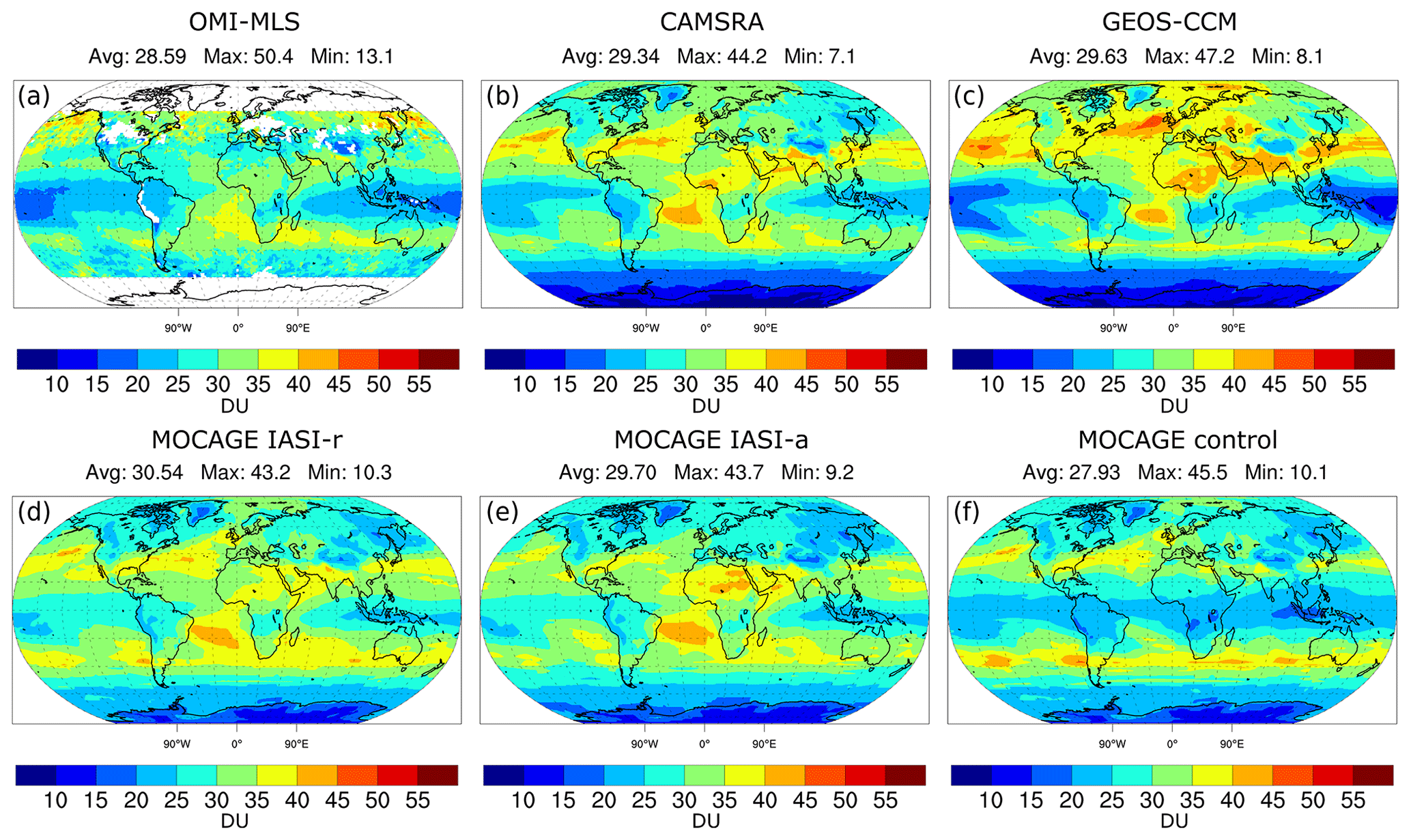
Figure 4 Tropospheric ozone column averaged over December–January–February 2010 from OMI-MLS retrievals (a), CAMSRA reanalysis (b), GEOS-CCM simulation (c), IASI-r reanalysis (d), IASI-a reanalysis (e), and the MOCAGE control simulation (f). Mean, minimum, and maximum values of ozone (in DU) are depicted over each plot.

During DJF months (Fig. 4), the global TOC is the lowest (28.6 DU for OMI-MLS retrievals). IASI-r, IASI-a, and CAMSRA show slightly higher TOC values than OMI-MLS but a rather similar geographical distribution to OMI-MLS and among each other. The GEOS-CCM model shows larger TOC maxima and lower minima with respect to the other models and OMI-MLS. The MOCAGE control simulation shows less pronounced zonal variability than all other models, which is expected due to the missing tropospheric chemistry description. The visible zonal structures in the control simulation are mostly a result of the zonal variability in the tropopause height.

Figure 5 Tropospheric ozone column averaged over March–April–May 2010 from OMI-MLS retrievals (a), CAMSRA reanalysis (b), GEOS-CCM simulation (c), IASI-r reanalysis (d), IASI-a reanalysis (e), and the MOCAGE control simulation (f). Mean, minimum, and maximum values of ozone (in DU) are depicted over each plot.

An increase in TOC is observed in the NH mid-latitudes during MAM months (Fig. 5). Values of TOC larger than 40 DU are observed with OMI-MLS over populated continental regions as well as over oceans. Larger TOC values are predicted by CAMSRA and GEOS-CCM compared with MOCAGE-based simulations and OMI-MLS. Due to the small sensitivity of IASI IR observations to the boundary layer O₃, IASI-r and IASI-a share the same limitations as the control simulation, i.e. a relaxation toward a zonal O₃ climatology in the lowermost model layers that is negatively biased (Emili et al., 2014). Such biases do affect the TOC computation to a limited extent. Nevertheless, IASI-r provides slightly larger TOC values than IASI-a, which seems more coherent with full-chemistry models and ozonesondes (Fig. 3). The decrease in TOC in the SH during the MAM months is reproduced by all models.

Figure 6 Tropospheric ozone column averaged over June–July–August 2010 from OMI-MLS retrievals (a), CAMSRA reanalysis (b), GEOS-CCM simulation (c), IASI-r reanalysis (d), IASI-a reanalysis (e), and the MOCAGE control simulation (f). Mean, minimum, and maximum values of ozone (in DU) are depicted over each plot.

During the JJA period (Fig. 6), values of TOC reach the maximum in the NH mid-latitudes with local maxima in the Mediterranean region, Southeast Asia, and China. As noted previously, GEOS-CCM tends to provide larger TOC variability and extrema. IASI-r and CAMSRA provide the best match to OMI-MLS measurements in this period of the year, whereas IASI-a and the control simulation underestimate the TOC. The increase in TOC in the SH tropical and mid-latitudes with respect to the MAM period is reproduced by all models except for the control simulation.

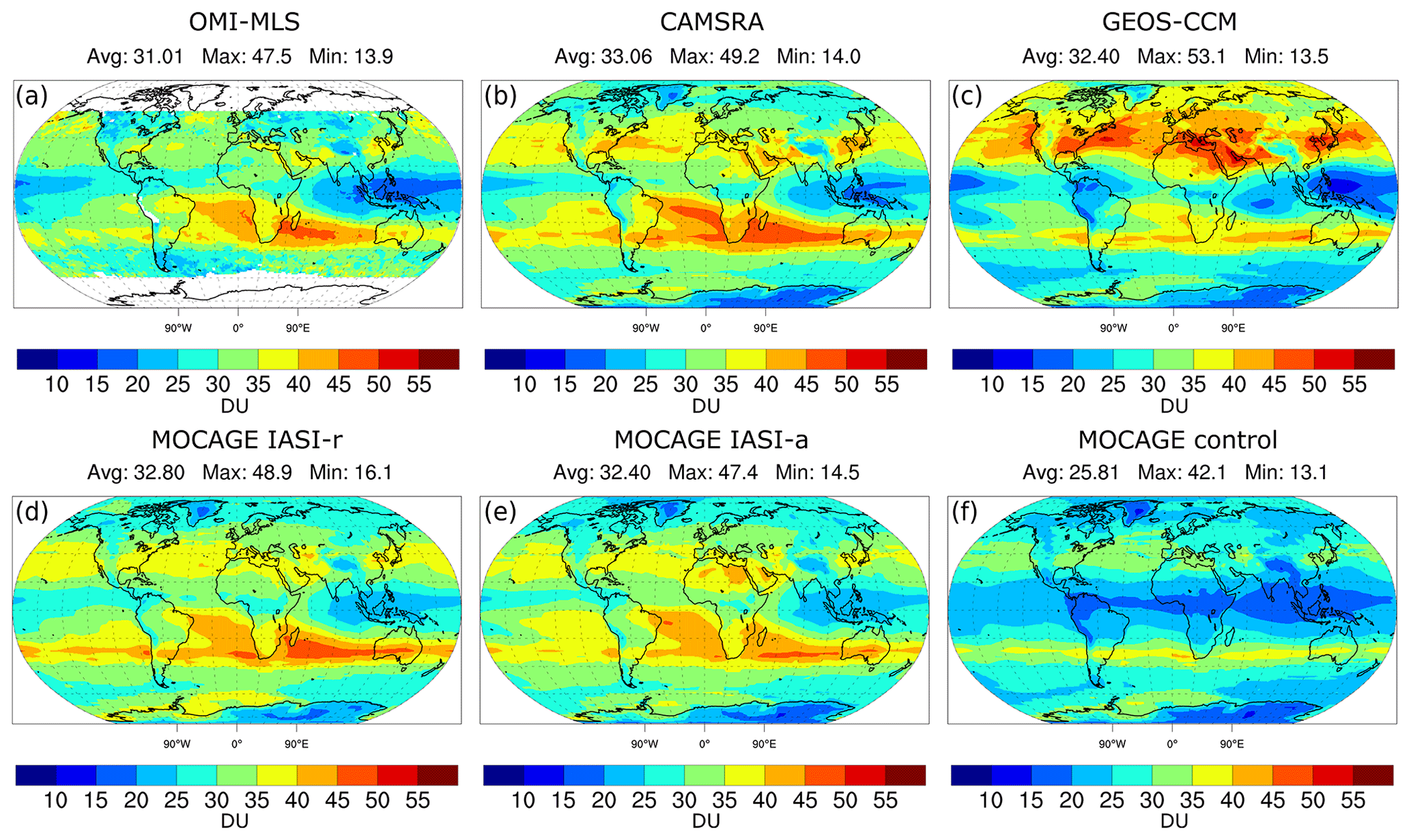
Figure 7 Tropospheric ozone column averaged over September–October–November 2010 from OMI-MLS retrievals (a), CAMSRA reanalysis (b), GEOS-CCM simulation (c), IASI-r reanalysis (d), IASI-a reanalysis (e), and the MOCAGE control simulation (f). Mean, minimum, and maximum values of ozone (in DU) are depicted over each plot.

In the SON months (Fig. 7), the TOC decreases significantly in the NH but increases in the SH, with a well-known local maximum stretching from the southern Indian Ocean to the Atlantic Ocean (Liu et al., 2017). IASI-r, CAMSRA, and, to a lesser extent, IASI-a, provide TOC distributions that match quite well with OMI-MLS measurements. GEOS-CCM simulates a smaller SH maximum and overly large TOC values in the NH mid-latitudes. On the other hand, the MOCAGE control simulation underestimates TOC values at all latitudes and does not reproduce the expected regional variability.

Finally, we remark that both IASI-r and IASI-a slightly overestimate TOC values inside the tropical deep convergence zone in Southeast Asia. This behaviour is observed for all periods of the year.

Overall, IASI-r and CAMSRA TOC values are the closest to OMI-MLS measurements, both in terms of regional variability and amplitude as well as for most of 2010. IASI-a TOC shows similar global patterns to IASI-r but with reduced amplitude, as anticipated from the previous section (Fig. 3).

5.3 Ozone ENSO index

We computed the O₃ ENSO index (Ziemke et al., 2011) for the ensemble of the O₃ analyses that are discussed in this study and compared it to the index derived directly from OMI-MLS observations. The O₃ ENSO index is defined as the difference (in DU) between the average tropospheric O₃ column in Southeast Asia (15^∘ S–15^∘ N and 70–140^∘ E) and in the Pacific Ocean tropical band (15^∘ S–15^∘ N and 180–110^∘ W). The O₃ ENSO index is strongly correlated with ENSO variability and has already been used to evaluate the capacity of CTMs and CCMs to reproduce tropical O₃ variability (Ziemke et al., 2015; Peiro et al., 2018).

This comparison does not represent an independent validation for CAMSRA, where both MLS and OMI measurements are assimilated. Nevertheless, it offers a useful benchmark for the other simulations presented in this study.

In Fig. 8, we report the O₃ ENSO index for 2010. As expected and already discussed by Peiro et al. (2018), the control simulation is not able to reproduce the O₃ ENSO signal observed by OMI-MLS, especially concerning the positive phase of the index. IASI-a has a good variability but a slightly negative bias, which was already diagnosed by Peiro et al. (2018) for reasons that were not clear at that time. GEOS-CCM displays smaller biases but a shift of 1 or 2 months concerning the transition between the positive and negative ENSO phases. IASI-r shows both small bias and a remarkably good correlation with OMI-MLS. Similar considerations can be given for CAMSRA reanalysis.

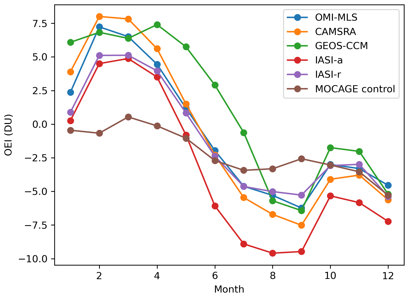
Figure 8 Ozone ENSO index (OEI) from OMI-MLS measurements (blue line), CAMSRA reanalysis (orange), GEOS-CCM simulation (green), IASI-a reanalysis (red), IASI-r reanalysis (violet), and the MOCAGE control simulation (brown).

To summarize, IASI-r improved the description of tropical O₃ variability linked to ENSO with respect to IASI-a, and it performs very similarly to CAMSRA, which has a full description of tropospheric chemistry and constrains tropospheric O₃ due to the simultaneous assimilation of both OMI and MLS. The new results also suggest that the bias of IASI-a could be linked to the limits of the empirical bias correction adopted by Emili et al. (2014) and Peiro et al. (2018) when assimilating IASI L2 retrievals. This problem is avoided with the direct assimilation of L1 radiances.

5.4 Comparison of ozone monthly fields

In Fig. 9, we present zonal averages of O₃ concentration as a function of altitude and month. The figure reports the temporal variability in monthly O₃ profiles at different latitudes (see panel headings) for CAMSRA (first column) as well as the difference between IASI-r, IASI-a, GEOS-CCM, the MOCAGE control simulation and CAMSRA (from left to right; see panel headings). CAMSRA, which is based on both comprehensive tropospheric chemistry and satellite assimilation, is considered here as the reference to be matched by the other systems.

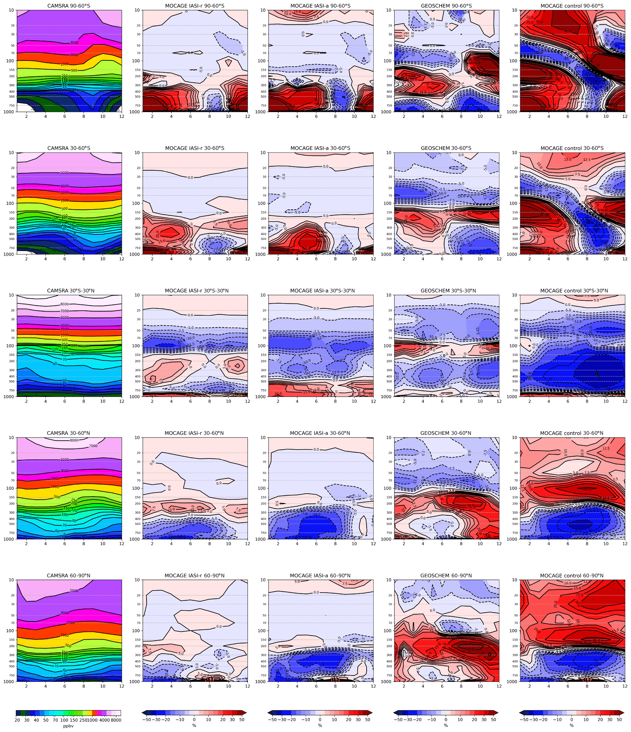
Figure 9 Ozone zonal averages as a function of month (x axis) and altitude (y axis, in hPa) for five respective latitude bands: 90–60^∘ S, 30–60^∘ S, 30^∘ S–30^∘ N, 30–60^∘ N, and 60–90^∘ N (see panel headings). CAMSRA O₃ (in ppbv) is plotted in the first column. The relative differences between IASI-r (second column), IASI-a (third column), GEOS-CCM (fourth column), the MOCAGE control simulation (fifth column) and CAMSRA O₃ are given as a percentage of the CAMSRA O₃.​​​​​​​

In the stratosphere (10–150 hPa), the differences between CAMSRA and IASI-r are smaller than 5 %, except close to the tropical tropopause, where they top at about 20 %. On the other hand, the differences between CAMSRA and our control simulation are significantly larger at all latitudes (up to 50 %). We can conclude that the strong similarities in stratospheric O₃ between CAMSRA and IASI-r are a consequence of assimilating MLS profiles in both reanalyses and of not of employing the same chemical mechanism (Cariolle and Teyssedre, 2007). The differences at the tropical tropopause might be linked to the different vertical resolution or assimilation configuration, which are expected to play a more significant role where O₃ vertical gradients are strong and concentrations are small. The GEOS-CCM simulation, which employs a detailed stratospheric O₃ chemical mechanism but does not assimilate any data, shows a persistent negative bias with respect to CAMSRA or IASI-r (of about 5 %–10 %). Note that the occurrence of the South Pole O₃ depletion starting in September is significantly underestimated in the control simulation, as well as by GEOS-CCM.

In the free troposphere (250–750 hPa), the control simulation has a predominant negative bias (up to 30 %) in the tropics and in the NH, whereas biases change sign as a function of altitude and month in the SH. These biases are in accordance with previous studies (Emili et al., 2014) and Fig. 3, and they are a consequence of the missing tropospheric mechanisms in the linearized chemical scheme. GEOS-CCM shows smaller differences with CAMSRA, but systematic negative biases are found in the tropics (10 %–15 %). In the NH, a positive bias initially localized in the upper troposphere (30 %–40 % between 150 and 400 hPa) spreads to the whole troposphere later in the year. Differences between IASI-r and CAMSRA are smaller at almost all latitudes with respect to the control simulation and GEOS-CCM, except in the lowermost layers (below 750 hPa), where IASI measurements do not provide sensitivity. Absolute differences with CAMSRA are lower than 10 % at all latitudes and seasons, except in the SH and springtime period.

IASI-a results are reported for completeness (Fig. 9, third column), and their comparison with IASI-r (second column) is coherent with previous findings (Sect. 5.1): IASI-r significantly reduced the tropospheric biases of IASI-a at mid-latitudes and high-latitudes, both in the SH and NH. Absolute differences between IASI-r/IASI-a and CAMSRA remain of the same order (10 %) in the tropics but differ in sign as a function of altitude and month.

To summarize, the monthly variability in O₃ profiles provided by IASI-r is the closest to that of CAMSRA. As the assimilation of MLS measurements does not influence the O₃ profiles below 300 hPa (Emili et al., 2014, 2019), we can conclude that the significant reduction in the tropospheric biases with respect to the control simulation during the entire year is a consequence of IASI assimilation. Due to the good coverage of IASI measurements, IASI-r also provides smaller differences with CAMSRA than GEOS-CCM, which employs a comprehensive chemical mechanism but is not constrained by satellite observations in this study.

6 Conclusions

The objective of this study was to re-evaluate the impact of IASI IR measurements on global tropospheric O₃ analysis, following recent improvements in methodological aspects concerning the data assimilation scheme (Emili et al., 2019; El Aabaribaoune et al., 2021). In particular, we recomputed the O₃ reanalysis of Peiro et al. (2018) for the year 2010, but we directly assimilated IR radiances from IASI instead of Level 2 retrievals. We named the new reanalysis IASI-r as opposed to IASI-a of Peiro et al. (2018), which shows little or no benefit from IASI assimilation in the extra-tropics. Most aspects of the system (e.g. chemical transport model, assimilation of stratospheric O₃ from MLS) were kept unchanged with respect to IASI-a in order to primarily evaluate the impact of the radiances assimilation. Some adjustments of the background error covariance were also performed, although they only produced a minor impact on reanalysis results.

IASI-r was first validated against ozonesondes, and the scores were compared with those of IASI-a. The scores of IASI-r and IASI-a are similar at tropical latitudes but are significantly better for IASI-r in the extra-tropics. The assimilation of IASI in this study improves the RMSE of the control simulation both in the SH mid-latitudes and in the NH polar region, whereas IASI-a was found to degrade the RMSE at these latitudes. The monthly variability in tropospheric O₃ columns confirms these findings and demonstrates that some positive seasonal signal can clearly be extracted from IASI at most latitudes. The only region where the impact is still neutral is between 60 and 90^∘ S, probably because of the difficulties involved in cloud screening and O₃ retrieval over elevated and icy surfaces.

Further analysis of IASI-r/IASI-a and two state-of-the-art modelling and data assimilation products (GEOS-CCM and CAMSRA) was conducted in the tropical region, by comparing the O₃ ENSO index. We found that IASI-r provides, along with CAMSRA, values of the ENSO index that are the closest to well-established satellite estimates (OMI-MLS) and significantly reduces the negative bias of IASI-a. We remind the reader that, while IASI-a already captured the O₃ variability in the tropics quite well, an empirical bias correction of Level 2 retrievals was necessary to avoid residual biases in the reanalysis (Emili et al., 2014). Residual biases in the O₃ index demonstrated the difficulties involved with such an approach. Within IASI-r, no observational bias correction has been performed and this was not found to be detrimental to the reanalysis. Barret et al. (2020) showed that the O₃ prior information used in L2 retrievals was likely a reason for some of the tropospheric biases previously found with IASI assimilation. The differences found between IASI-r and IASI-a in this study point to the same conclusion, i.e. that a dynamical O₃ prior information, which comes directly from the CTM forecasts in our case, is beneficial for the assimilation of IR measurements. In the future, it might be interesting to evaluate the assimilation of improved Level 2 retrievals (Barret et al., 2020) and see whether this also solves the issues previously encountered with IASI-a.

Finally, the temporal variability in vertical O₃ profiles from IASI-r, IASI-a, GEOS-CCM, and the MOCAGE control simulation (linearized O₃ chemistry) has been compared to that provided by the CAMSRA reanalysis, which has been extensively validated in other studies and has proven to be quite accurate. The monthly O₃ profiles of IASI-r are the closest to CAMSRA, confirming that a simple chemical mechanism in combination with the assimilation of both stratospheric and tropospheric O₃ sounders can provide similar performance to more complex set-ups. Thus, the methodology presented in this study could be useful to improve the tropospheric O₃ description in NWP systems (usually based on simplified O₃ chemistry), where IR measurements are already assimilated to constrain temperature and water vapour profiles. The additional cost of the RTM computations would, in this case, scale linearly with the number of added O₃-sensitive channels. In this work, we used the original spectral selection of Barret et al. (2011), but the presence of strong inter-channel error correlations (El Aabaribaoune et al., 2021) suggests the possibility to significantly reduce the number of assimilated channels without degrading the analysis. This represents an interesting area for further research.

The GEOS-CCM simulation, which is based on a comprehensive chemical mechanism but does not assimilate any satellite information in this study, sits between our control simulation and IASI-r. Hence, we advocate that assimilating IR measurements from IASI might also be beneficial for models that are based on more detailed O₃ chemistry. An evaluation of the added value of IASI assimilation within the CAMSRA system would also offer further insights into the relative importance of UV and IR sounders for tropospheric O₃ reanalyses.

A strong data thinning of IASI observations has been performed in this study to match the low resolution of the CTM (2^∘), which resulted in the rejection of many potentially informative IASI pixels. The small numerical cost of the CTM configuration permits an increase in horizontal resolution and, thus, the possibility to use significantly more satellite observations. A strong increase in the number of assimilated pixels might require an investigation of the presence and the potential implementation of spatially correlated observation errors, which are still neglected in most systems. Further improvements in IR O₃ assimilation might also come from simulating the effect of large aerosol particles (e.g. dust) in the radiative transfer computations. All of these aspects deserve to be considered in future studies.