the Creative Commons Attribution 4.0 License.
the Creative Commons Attribution 4.0 License.
 | 29 Jan 2021
Comparison of sea ice kinematics at different resolutions modeled with a grid hierarchy in the Community Earth System Model (version 1.2.1)
Jialiang Ma
Yan Zhang
Jiping Liu
Bin Wang
High-resolution sea ice modeling is becoming widely available for both operational forecasts and climate studies. In traditional Eulerian grid-based models, small-scale sea ice kinematics represent the most prominent feature of high-resolution simulations, and with rheology models such as viscous–plastic (VP) and Maxwell elasto-brittle (MEB), sea ice models are able to reproduce multi-fractal sea ice deformation and linear kinematic features that are seen in high-resolution observational datasets. In this study, we carry out modeling of sea ice with multiple grid resolutions by using the Community Earth System Model (CESM) and a grid hierarchy (22, 7.3, and 2.4 km grid stepping in the Arctic). By using atmospherically forced experiments, we simulate consistent sea ice climatology across the three resolutions. Furthermore, the model reproduces reasonable sea ice kinematics, including multi-fractal spatial scaling of sea ice deformation that partially depends on atmospheric circulation patterns and forcings. By using high-resolution runs as references, we evaluate the model's effective resolution with respect to the statistics of sea ice kinematics. Specifically, we find the spatial scale at which the probability density function (PDF) of the scaled sea ice deformation rate of low-resolution runs matches that of high-resolution runs. This critical scale is treated as the effective resolution of the coarse-resolution grid, which is estimated to be about 6 to 7 times the grid's native resolution. We show that in our model, the convergence of the elastic–viscous–plastic (EVP) rheology scheme plays an important role in reproducing reasonable kinematics statistics and, more strikingly, simulates systematically thinner sea ice than the standard, non-convergent experiments in landfast ice regions of the Canadian Arctic Archipelago. Given the wide adoption of EVP and subcycling settings in current models, it highlights the importance of EVP convergence, especially for climate studies and projections. The new grids and the model integration in CESM are openly provided for public use.
- Article
(21586 KB) - Full-text XML
-
Supplement
(1700 KB) - BibTeX
- EndNote


Sea ice is the interface between the polar atmosphere and ocean, and it is therefore an important modulating factor of polar air–sea interactions. The momentum input into the sea ice from the atmosphere and the ocean causes sea ice drift, as well as failures and deformations at a wide range of temporal and spatial scales. As revealed by high-resolution, kilometer-scale sea ice drift and deformation estimates with synthetic aperture radars, the deformation of sea ice is shown to be multi-fractal with scale-invariance properties (Marsan et al., 2004; Rampal et al., 2008; Weiss and Dansereau, 2017), and quasi-linear kinematic features are observed through visual inspection (Kwok et al., 2008), including local deformation regions of sea ice failures and shearing. Furthermore, the these kinematic features are accompanied by the formation of sea ice leads and pressure ridges tightly coupled to sea ice and polar thermodynamic processes. While sea ice leads are hot spots of heat and moisture fluxes during winter, sea ice ridging is responsible for producing the thickest sea ice in both polar regions.
Sea ice rheology models provide mathematical descriptions and numerical treatments for sea ice dynamic processes and are thus essential components of sea ice models. Viscous–plastic (VP; Hibler, 1979) is the most widely used rheology model, and it describes sea ice as a two-dimensional continuum with nonlinear viscosity, which undergoes plastic deformations over critical shearing and compressive stresses. In order to overcome the numerical stiffness of the VP model, modelers usually adopt explicit solvers for the derived VP models such as elastic–viscous–plastic (EVP; Hunke and Dukowicz, 1997), instead of the original VP, or implicit solvers (Hibler, 1979; Lemieux et al., 2010). With the introduction of an artificial term for elastic waves into the VP model, the numerical solving process is transformed into an explicit formulation. An iterative process, called subcycling, is carried out in EVP in order to numerically attenuate the elastic wave and obtain the solution to the VP model. Due to its good numerical stability and straightforward implementation, EVP is adopted by many climate models participating in the Coupled Model Intercomparison Project (CMIP6) and hindcast experiments for operational sea ice forecasts (Dupont et al., 2015).
With VP rheology, the capability of sea ice models to resolve fine-scale deformations is inherently bounded by the resolution of the models' grids. In order to reproduce the observed properties of the sea ice kinematics, grids of 0.1∘ resolution or finer in sea ice regions are usually required. State-of-the-art high-resolution studies reach 2 km or finer grid stepping in the Arctic (Hutter et al., 2018; Scholz et al., 2019). Although the continuum assumption of the sea ice cover in VP (or EVP) does not necessarily hold at these resolutions, VP models are shown to be capable of reproducing realistic sea ice kinematics (Hutter et al., 2018). Unstructured grid-based models and Lagrangian models have unique capabilities in modeling sea ice. Regionally focused studies can be easily carried out with variable grid sizes, such as the Arctic simulation with FESOM (Wang et al., 2018; Koldunov et al., 2019). Purely Lagrangian models such as neXtSIM (Rampal et al., 2019) are potentially free of the resolution issues for resolving small deformation features. Specifically, neXtSIM utilizes Maxwell elasto-brittle rheology (Dansereau et al., 2016; Girard et al., 2011), which is shown to simulate reasonable sea ice kinematics and scaling properties even at moderate-resolution settings (Rampal et al., 2019). Traditional VP rheology is limited due to the lack of memory for past deformation events (Hutter and Losch, 2020). There are also efforts to improve the rheology model in terms of simulating observed anisotropy in sea ice floe shape and associated deformation (Tsamados et al., 2013).
In this study, we carry out a comparison of sea ice model simulations at different spatial resolutions with the coupled Community Earth System Model (CESM, version 1.2.1). CESM (http://www.cesm.ucar.edu, last access: 20 December 2020) is developed at the National Center for Atmospheric Research (NCAR) and adopted by various research groups in the world for climate studies. The component models of CESM include the Community Atmospheric Model (CAM), the Parallel Ocean Program (POP, version 2), the Community Ice CodE model (CICE, version 4), and the Common Land Model (CLM). The coupling between these components is carried out with the flux coupler CPL. Components can be configured to the specific experiment needs, such as atmospherically forced ocean and (or) sea ice simulations. Figure 1 shows the coupling schematics in CESM and the common configuration of high-resolution coupled runs. The horizontal model grids (and associated spatial resolutions) of CICE and POP are the same, and the two standard configurations in CESM are nominal 1∘ (GX1V6, a dipolar grid) and 0.1∘ (TX0.1v2, a tripolar grid). Specifically, CICE, the sea ice component of CESM, includes comprehensive thermodynamic and dynamic processes of sea ice, including discretized ice thickness distribution, prognostic enthalpy, complex shortwave albedo and penetration schemes with snow and pond processes, an EVP model, and ridging parameterization. CICE in CESM can be run in three major settings: (1) forced by atmospheric reanalysis (NCEP CORE-2) with coupling to a slab ocean model (SOM), (2) ice–ocean coupled simulation under atmospheric forcings, and (3) fully atmosphere–ocean–ice coupled runs.
In our study, we design grid hierarchies for the ocean and the sea ice model and incorporate them into CESM, including the component models of CICE and POP, as well as the coupling to the atmospheric forcings. The grid hierarchy includes three tripolar grids with nominal resolutions of 0.45, 0.15, and 0.05∘, covering a wide range of climate modeling and sub-mesoscale-oriented studies. In Sect. 2 we introduce the grid generation method and the integration of the grid hierarchy in CESM. Furthermore, atmospheric-forcing-based experiments are carried out with the new grids, and Sect. 3 includes the details of the experiments and the analysis of modeled sea ice climatology and kinematics. We carry out scaling analysis and cross-resolution comparisons of the sea ice kinematics and study the convergence behavior of EVP. In Sect. 4 we summarize the article and provide a discussion of related topics for future research directions including multi-scale modeling.

Figure 1Ocean and sea ice grids and air–sea coupling in the Community Earth System Model (CESM).
2.1 TS grids – a tripolar grid hierarchy
We design a new grid hierarchy for global ocean–sea ice modeling. The generated grids are orthogonal and compatible with many existing ocean and sea ice models, including POP, CICE, and MOM. Following the methodology in Murray (1996) and Madec and Imbard (1996), we design and implement a grid generation method that ensures a smooth global transition of grid scales and supports direct model integration in POP and CICE. As shown in Fig. 2, it consists of two patches, the southern patch (SP) and the northern patch (NP), divided by a certain latitudinal circle (ϕ) in the Northern Hemisphere. For the SP, the grid lines are purely zonal or meridional. For the NP, there are two north poles for the grid, which are placed on the Eurasian and North American landmasses. However, unlike many tripolar grids such as TX0.1V2 in CESM, this new grid features a smooth grid-scale transition on the boundary of SP and NP. In order to achieve this, a non-trivial grid generation process is carried out on the stereographic projection of NP. Specifically, a series of embedded ellipses is constructed based on resolution requirements, with (1) the outermost ellipse as the projection of the latitudinal circle at ϕ (i.e., a circle) and (2) the innermost ellipse as the line linking the two grid poles. The foci of the outermost ellipse are both at the North Pole; with the progression to inner ellipses, they gradually move towards the two grid poles. The ellipses form the “zonal” grid lines in NP. After the ellipses are constructed, the “meridional” grid lines in NP are constructed, starting from the southern boundary of NP, down to the innermost ellipse. During this process, it is ensured that (1) the grid lines are constructed consecutively between adjacent ellipses, with starting points on the outer ellipse, and (2) they are linked with the meridional grid lines in SP to ensure overall continuity of the global grid. The details of the construction of ellipses and the smooth transition of meridional grid scales are further described in Appendix A. Furthermore, the meridional grid scales in both SP and NP are constructed to alleviate the grid aspect ratio, reducing meridional grid sizes at higher latitudes.
By using the grid generation method, we generate a series of tripolar grids: TS045, TS015, and TS005. These grids all have a boundary between SP and NP (ϕ) at 10∘ N, with grid poles at 63∘ N, 104∘ W and 59.5∘ N, 76∘ E. Table 1 shows the detailed configuration of these grids. TS045 is the coarsest grid with a nominal resolution of 0.45∘, and it targets climate modeling and the typical resolution range for ocean component models in the Coupled Model Intercomparison Project (CMIP6). TS015 and TS005 are about 3 times (or nominal 0.15∘) and 9 times (or nominal 0.05∘) the resolution of TS045, respectively.
Figure 3 shows the horizontal grid scale () in polar regions for TS015 and TS005. The average grid scale in TS005 is 2.45 km in the Arctic oceanic regions (north of 65∘ N), and the scales of TS015 and TS045 are 7.34 and 22.01 km, respectively. From the ocean modeling perspective, we use the Rossby deformation radius (R) as a proxy for the mesoscale (Chelton et al., 1998) and investigate the capabilities of each grid. Specifically, the criterion in Hallberg (2013) is adopted: mesoscale-resolving capability is attained when s is smaller than half of the local value of R. Based on the annual mean WOA13 climatology of salinity and temperature (Locarnini et al., 2013; Zweng et al., 2013), we construct the global distribution of R. In Table 1 we note that TS015 is “almost eddying” because this grid is mesoscale-resolving for 65 % of the global ocean area. As outlined in Fig. 3, in polar regions, the ratio of s to R is higher than 0.5 for TS015, indicating no mesoscale-resolving capability for this grid for these regions. But for TS005, the mesoscale processes in polar regions with relatively deep bathymetry (e.g., within the Arctic Ocean) can be resolved.

Figure 2Global tripolar TS grid with the northern patch (in cyan) and southern patch (in black). The 0.05∘ grid (TS005) is shown (1 in every 60 grid points). On the boundary of the two patches, smooth grid size change is ensured in the meridional direction. Typical meridional grid lines are also shown as thick lines (red, green, and blue).
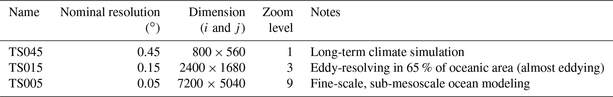
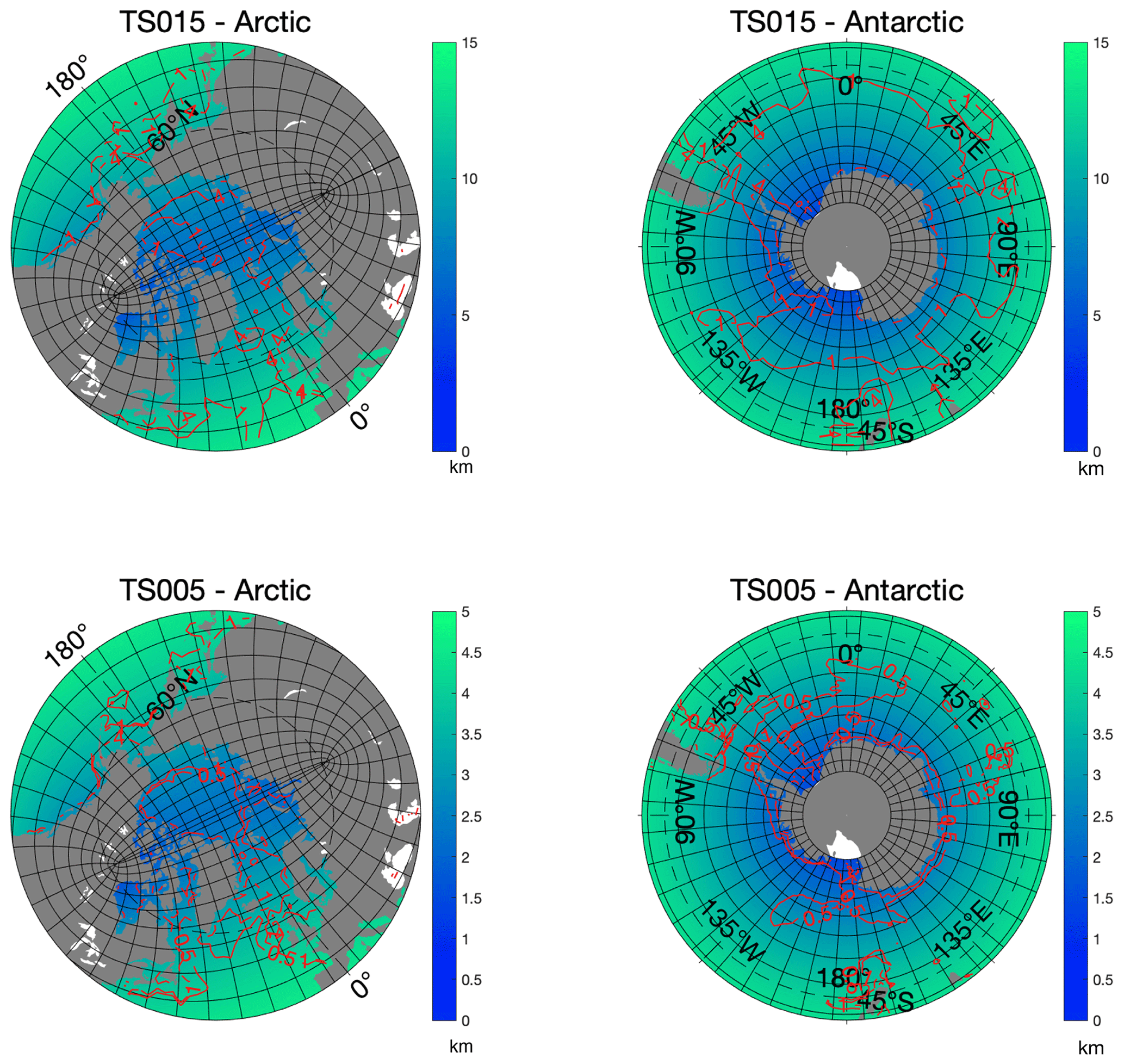
Figure 3Horizontal grid scale of TS015 and TS005 in the polar regions. For grid lines, 1 in 60 (or 180) points is shown for the TS015 (or TS005) grid. is shown by filled contours (in kilometers), and regions of mesoscale-resolving capability () are outlined by red contour lines.
2.2 TS grid integration in CESM
The integration of the TS grids in CESM involves the following three steps. The first is the generation of land–sea distribution and bathymetry, as well as the technical implementation of the grids in both POP and CICE. Model bathymetry is generated at the grid locations and 60 vertical layers based on the ETOPO1 dataset (ETOPO1, 2019). The vertical coordinate consists of 10 m equal depth layers in the top 200 m, with a gradual increase in layer depth to 250 m in the deep oceans (up to 5500 m).
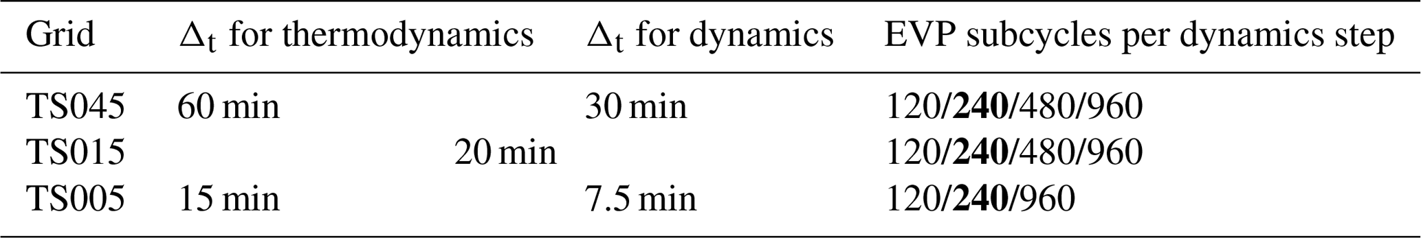
Second, we configure the model according to the grid resolution, including the choice of parameterization schemes and related parameters. Specifically, we adopt the full thermodynamic and dynamic model processes in CICE, mainly following the standard configurations of parameterization schemes in Hunke and Lipscomb (2008). The main processes relating to sea ice dynamics include an EVP rheology model (Hunke and Dukowicz, 1997), the ridging–rafting scheme (Lipscomb et al., 2007) and ice strength model (Hibler, 1979), and transport-remapping-based advection (Dukowicz and Baumgardner, 2000). Model configuration and parameters are aligned across the three grids, with details shown in Appendix B. The major difference among the grids is that we choose shorter thermodynamics and dynamics time steps for grids with higher resolution (Table 2). Furthermore, since sea ice kinematics are the focus of this study, different EVP subcycle numbers are chosen for each grid. While 120 subcycles per hour is adopted for some 1∘ resolution CMIP simulations (Jahn et al., 2012; Xu et al., 2013), we experiment with larger values of cycle counts (up to 960 subcycles per dynamic time step), as shown in Table 2.
In our study, CICE is coupled to the slab ocean model (SOM) in CESM, which provides a climatological seasonal cycle of ocean mixed layer depth and heat potential. The same configuration for SOM is used for experiments with TS045, TS015, and TS005. The reason we use SOM instead of a fully dynamic–thermodynamic ocean model (such as POP) is three fold. First, in this study we focus on the simulation of sea ice kinematics and the intercomparison across different resolution settings. Therefore, by using a single-column model for the ocean, we eliminate the factors that may compromise comparability, including the inconsistency in modeled ocean processes across the resolution range, as well as ocean and coupled turbulence. Second, since atmospheric forcing is the major driver of sea ice drift and kinematics, we consider SOM applicable for the purpose of this study. Third, using SOM with CICE in CESM greatly alleviates the computational overhead for long-term simulations, especially for TS005 (0.05∘ grid). As shown in the next section, with CICE coupled to SOM, we simulate comparable Arctic sea ice climatology and kinematic features (cracking events, etc.) among TS045, TS015, and TS005, and the computational cost and time to solution remain manageable. Potential compromises pertaining to the use of SOM are discussed further in Sect. 4.
Fourth, we force the sea ice component with TS grids with atmospheric forcings from the CORE-2 dataset, which is also used in the Ocean Model Intercomparison Project (Griffies et al., 2016). Specifically, the CORE-2 dataset contains a normal-year forcing (NYF) with the climatological annual cycle based on NCEP atmospheric reanalysis, and it has a spatial resolution of about 2∘ (T62) with 4 times the daily wind stress fields. The NYF dataset is mainly based on the year 1995 of the NCEP atmospheric reanalysis, with interpolation-based smoothing at the end of December with data from the year 1994 and flux corrections to ensure overall energy balance. Following the common practice in CESM, for the coupling of atmospheric state variables (such as air temperature and humidity), a bilinear interpolator is used between T62 and each TS grid. For wind stress, the patch-recovery algorithm is adopted to ensure good structure of wind fields on the ocean–sea ice grid. Patch recovery is a high-order interpolation method based on local reconstruction of the forcing fields, and it ensures consistent wind stress forcing across the three grid resolutions in this study. For fluxes, a first-order conservative interpolator is utilized. All these interpolators (in total six) are generated through the CESM mapping toolkit and ESMF regridding toolkit (https://www.earthsystemcog.org/projects/esmf/, last access: 20 December 2020).
All the model integrations for TS grids in CESM, including grid files in the format of POP and interpolation files, are openly available (details in the “Code and data availability” section).
Table 2Time stepping and EVP configurations; 240 (in bold) is the default value for EVP subcycles for each dynamics step during the long-term spin-up experiments. Other values, including 120, 480, and 960, are also used for the comparative study of modeled sea ice kinematics.
3.1 Spin-up experiments and Arctic sea ice climatology
The spin-up simulations with the new grids are based on CESM D-type experiments and configured specifically for each grid. CESM D-type experiments are based on the CORE-2 NYF dataset and coupling to SOM, and they are usually used for spin-up for the sea ice and ocean–sea ice coupled system. For CICE, the time stepping is based on 240 EVP subcycles (i.e., the number of time steps for elastic wave damping, or NDTE) per dynamics time step for all three grids, following the settings in Table 2. The experiments are outlined in Fig. 4a. Specifically, the experiment with TS045 starts on 1 January with no sea ice, and the model gradually reaches an equilibrium state for both sea ice coverage and volume. After the 25-year experiment with TS045, the spun-up status is migrated onto TS015. Similarly, after another 5-year experiment with TS015, the spun-up status is further migrated onto TS005. We carry out the analysis of Arctic sea ice climatology based on experiments with the default value for NDTE (240) for TS045, TS015, and TS005. The experiments with other values for NDTE show little difference in overall sea ice coverage and volume, but they greatly impact the modeling of kinematics (details in Sect. 3.2).
As shown in Fig. 4b, for TS045, the Arctic sea ice extent (SIE) and volume (SIV) approach equilibrium after about 5 and 30 years, respectively. With a migrated status from experiments with lower-resolution grids, the runs with TS015 and TS005 attain a quasi-equilibrium status towards the end of the 37th model year. The annual cycles of the sea ice coverage, computed as the mean monthly SIE and SIV of the last 5-year model output, agree well among the three grids (Figs. 4b and 5a). The differences in SIE and SIV are within 5 %. The spatial distributions of sea ice are also consistent (Fig. 5c–h). The model results are also in good agreement with observational climatology of the seasonal cycle for sea ice extent (NSIDC sea ice index, years 1979 to 2002), with a minor overestimation of the sea ice coverage during winter (Fig. 5a). As shown in Fig. 5f–g, the overestimation in March is present in outer regions to the Arctic Ocean, including the Okhotsk Sea, Labrador Sea, the southern part of the Greenland Sea (near Iceland), and the southern part of the Barents Sea. During summer when the sea ice coverage is mainly present within the Arctic Basin, all three grids reproduce reasonable sea ice coverage regarding observations (Fig. 5c–e).
The modeled SIV peaks in April (Fig. 5b), and the modeled seasonal cycle is consistent with existing sea ice thickness reconstructions of PIOMAS (Schweiger et al., 2011). The overall thickness pattern shows thick ice (over 3 m) in the regions north of the Canadian Arctic Archipelago (CAA) and Greenland, as well as within CAA. Among the three grids, higher-resolution grids simulate a slightly higher sea ice volume by the end of winter (by only 4 %), which is seen in the central Arctic (Fig. 5f–h). During summer and the early months of the winter, all three grids simulate lower SIV compared against PIOMAS (Fig. 5b), with one particular region showing an underestimation of ice thickness in the Atlantic sector of the Arctic (Fig. 5c–e). In general, we consider the model to simulate reasonable Arctic sea ice climatology, especially during winter. Furthermore, with good consistency across the three resolutions, we carry out an analysis of sea ice kinematics with high-frequency outputs of these experiments.
One major obstacle to running high-resolution models is the huge amount of computational overhead and the long durations for climate simulations. In this study, we utilize an Intel-processor-based cluster with 24 cores per node for all the experiments. For TS045 and TS015, more than 5 simulated years per day (SYPD) can be attained with fewer than 1000 cores for all the experiments. For TS005, the simulation speed is about 1 SYPD with 1920 cores and NDTE 240, which is reasonable given the high resolution of the grid. The utilization of larger computational facilities for TS015 and TS005 remains an important direction of future work.
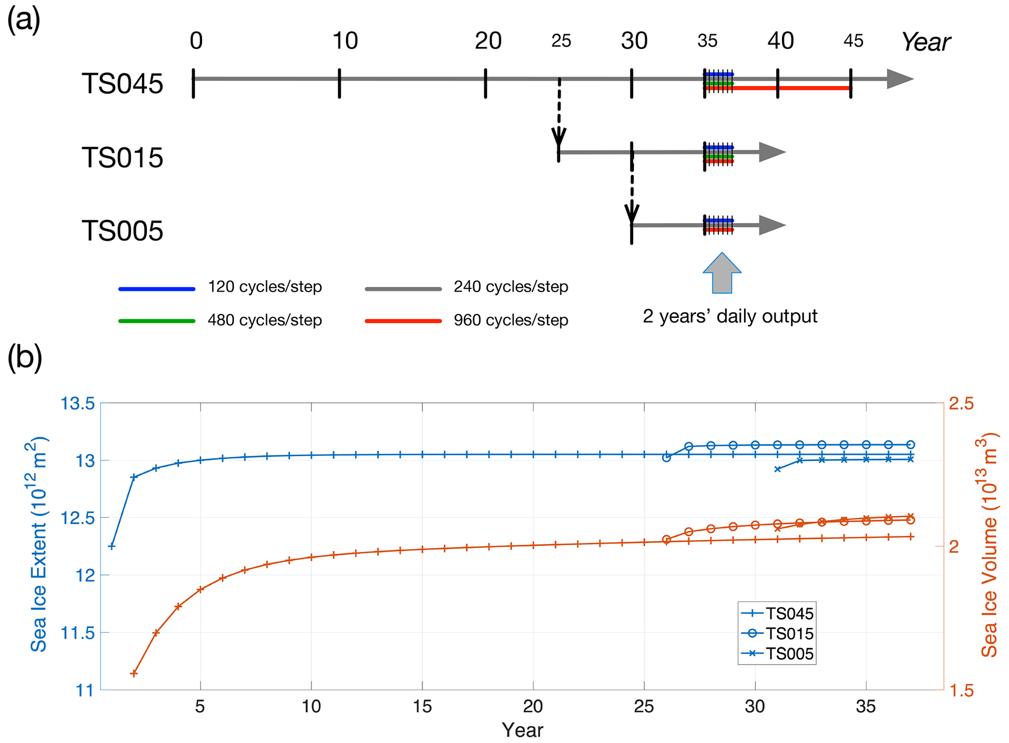
Figure 4Spin-up experiments of sea ice simulations with TS grids (a) and spin-up of Arctic sea ice extent and volume (SIE and SIV, in panel b) up to year 37. These experiments are based on D cases in CESM: the sea ice component CICE is forced with normal-year forcing of CORE and coupled to the slab ocean model. For TS045, the model is initialized with an ice-free condition, and the numerical integration is carried out until equilibrium. For TS015, a snapshot of the spun-up conditions of TS045 at the end of year 25 is used to initialize the integration, and the experiment is carried out for 12 years up to year 37. For TS005, a snapshot of the spun-up status of TS015 at the end of year 30 is used for model initialization, and the experiment is carried out for 7 years up to year 37.
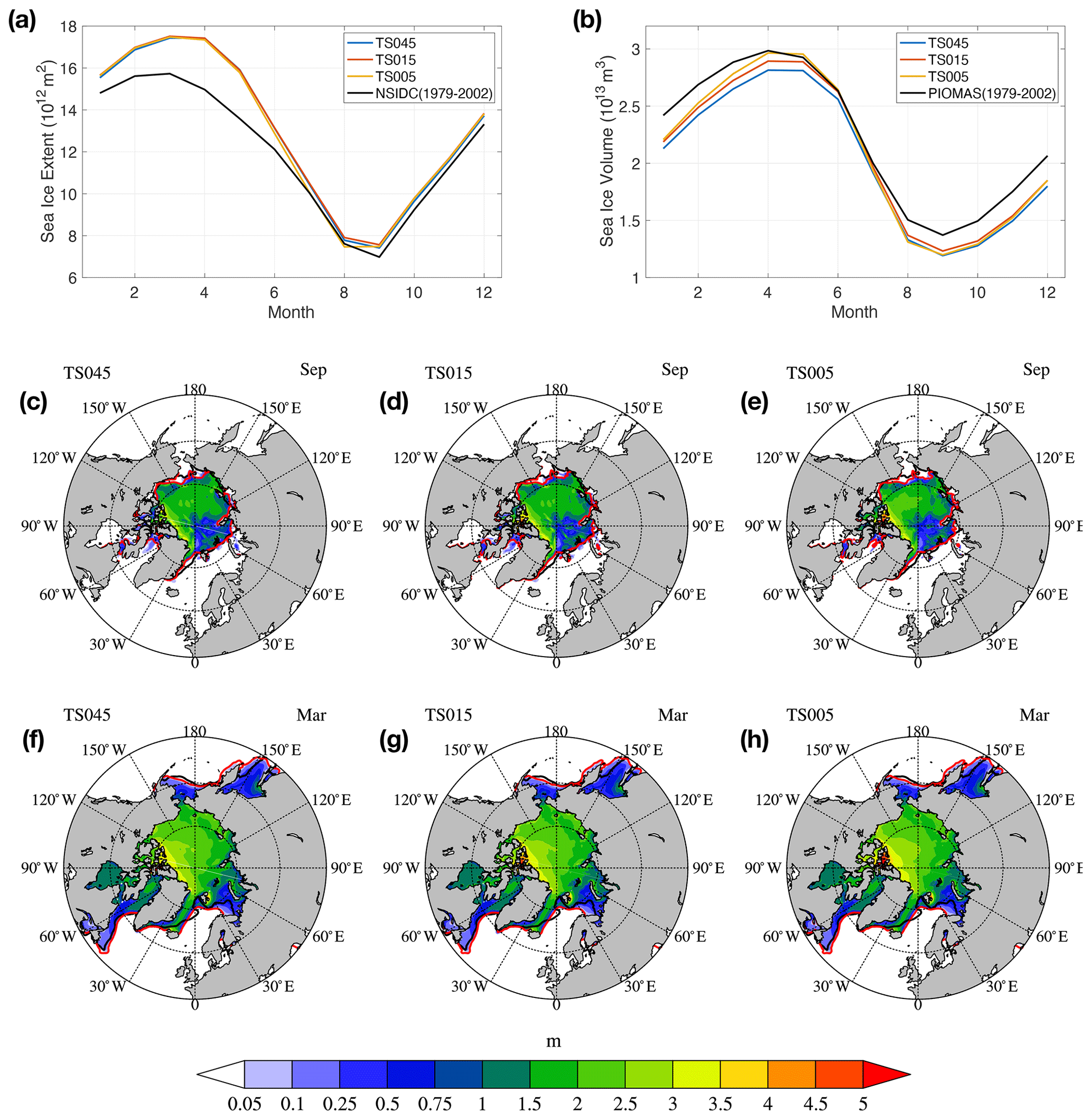
Figure 5Climatological seasonal cycle of Arctic SIE (a) and SIV (b) computed as a 5-year mean of years 33 to 37. September (or March) sea ice thickness fields for TS045, TS015, and TS005 are shown in panels (c) (or f), (d) (or g), and (e) (or h), respectively. Within each panel (c–h), the satellite-observed and modeled sea ice edge (sea ice concentration at 15 %) are marked by black and red lines, respectively. The climatology SIE values, as well as March and September sea ice edge, are computed from the NSIDC Arctic sea ice dataset from passive microwave sensors (SSMI–SMMR) for the years between 1979 and 2002. The climatological annual cycle for SIV (in panel b) is computed from the PIOMAS dataset for the same period (1979 to 2002).
3.2 Sea ice kinematics and scaling on representative days
In order to study the sea ice kinematics, we output 2 years (36–37) of daily mean sea ice fields for all three TS grids (Fig. 4a). Spatial scaling analysis of these deformation rates is performed by using the methods in Marsan et al. (2004). The deformation rates in their invariant forms are defined in Eqs. (1) through (3), including shearing rate (), divergence rate (), and total deformation rate (). They are computed from the daily mean prognostic sea ice drift speeds (u and v) defined on Eulerian grid locations (with Arakawa-B staggering in CICE). Specifically, the line integral of a specified model region is computed for the spatial derivatives and the associated spatial scale (Fig. C1). The deformation rates are then computed and binned according to the specific spatial scale in order to derive statistics including the probability density of deformation rates at different scales. Appendix C includes a detailed routine for the Arakawa-B staggered grid of CICE.
We have manually chosen two typical days that are representative of Arctic sea ice drift patterns: 20 December and 6 February (Fig. 6a and b). A wintertime Arctic oscillation (AO) index is constructed based on sea level pressure (SLP) of 50-year NCEP reanalysis data and applied to the NYF dataset. Specifically, AO is defined as the leading empirical orthogonal function (EOF) mode for the weekly mean SLP in the Northern Hemisphere (20∘ N and north) for the extended winter months (November to April) in the years 1950 to 2000. The 50-year SLP sequence is detrended and the seasonal cycle is removed for the EOF computations. The leading mode explains 13.9 % of the total variance, with the normalized spatial pattern (unitless) and the principal component (time series) shown in Fig. S1 in the Supplement. The wintertime AO index of the NYF dataset is shown in Fig. 6c. The winter of the NYF forcing dataset corresponds to an overall neutral AO status, and the variability of the wintertime weekly AO index (25 hPa as in Fig. 6c) is also on par with the average intra-seasonal variability of the 50-year NCEP reanalysis data (22 hPa as in Fig. S1b). As a reference, the summertime AO of the NYF dataset is mildly negative (Fig. S1c).
The two representative days are (1) 20 December, on which the high-pressure center resides in the Beaufort Sea and a negative AO index is seen, and (2) 6 February, on which the high-pressure center shifts towards the Eastern Hemisphere, the low-pressure system in the Atlantic sector extends further into the Arctic, and a slightly positive AO index is present. Furthermore, because asymptotic convergence of sea ice kinematics to increase in the EVP subcycle count is seen in existing studies (Lemieux et al., 2012; Koldunov et al., 2019), we limit the analysis of kinematics and scaling to the experiments with the largest EVP subcycles (NDTE = 960) for each grid.
Figure 7 shows the deformation fields for 20 December. On the Pacific side, there is divergence in the Beaufort Sea and Chukchi Sea, with accompanying convergence in the East Siberian Sea. A shearing rate up to 10 % d−1 is also present in these regions, with a shearing arc extending from the Beaufort Sea across the basin to Severnaya Zemlya and another one along the Siberian Shelf. In the Atlantic sector of the Arctic Ocean, there is extensive divergence to the north of Svalbard and minor convergence to the north of Greenland. In the regions of thinner ice and marginal ice zones, large deformation rates are present.
The overall deformation pattern on 20 December is consistent across TS045, TS015, and TS005. Comparing TS045 and TS015, we witness much finer structure of the deformation fields in all aforementioned regions. Specifically, narrower shearing and divergence regions as well as higher deformation rates are present in TS015. The differences in the kinematics between TS015 to TS005 are mainly present in the fine structure of the deformation and shearing events. With TS005, the model simulates more and finer sea ice kinematic features, such as the network of shearing in the Beaufort Sea and along the Siberian Shelf.
Figure 8 shows the deformation fields for 6 February. On the Pacific side, the divergence (convergence) region is in the Beaufort Sea (Chukchi Sea). The divergence in the Laptev Sea is paired with the convergence to the north of the Queen Elizabeth Islands (see Fig. 6b for the sea ice drift). A shearing belt is present across the basin from the Canadian Arctic Archipelago to the north of Franz Josef Land. In the Atlantic sector, the convergence to the north of the Barents Sea corresponds to the divergence in the north, including the north of Greenland and the north of Franz Josef Land. The simulation results are consistent across the three grid resolutions, including the major regions of divergence (or convergence) and those of shearing, except for very large shearing belts across the basin.
Similar to 20 December, TS045, TS015, and TS005 simulate consistent deformation fields, including the location and strength of deformation events in the Arctic Basin. There is a clear separation of the level of detail for the deformation systems across resolutions. The kinematic features that can be detected by visual inspection are better defined in TS005. The networks of deformations, such as those in the Davis Strait and to the north of Fram Strait and Greenland, contain over 20 major linear features in TS005. For comparison, the run with TS015 produces much fewer features, while that with TS045 only produces the one or two major deformation features. However, on both days, there is also evidence that, even at TS005, the model is limited in resolving fine-scale kinematic structures. Some large kinematic features, especially in the central Arctic, have ends that are not well-defined, which is clearly not bounded by the grid sizes. This applies to both shearing and divergence. On the grid's native resolution, the simulated kinematic features contain both physical deformation and the deformation caused by numerical issues, such as the limitation of grid resolution and non-convergent solutions. As a consequence, the effective resolution of the model is usually coarser than the grid's native resolution, which we further evaluate using statistics on sea ice deformation.
We examine the probability density function of total deformation rates, which were previously investigated for RADARSAT Geophysical Processor System (RGPS) data (Marsan et al., 2004). Specifically, the region outlined in Fig. 7 is used for the study, and we show the daily and 3 d cumulative probability density function (PDF) for total deformation rates in Fig. 9. The 3 d deformation data are computed from the 3 d mean velocity fields for the periods of 19–21 December and 5–7 February, respectively. With higher resolution, the model consistently simulates more extreme deformation events corresponding to a flatter cumulative PDF for the deformation rates.
Since the three grids have a nearly exact grid stepping ratio of , we carry out (1) the spatial coarsening of the model output of TS005 onto TS015 and TS045 and (2) that of TS015 onto TS045. The cumulative PDFs for each resolution, including those modeled with the native resolution and those scaled from higher resolutions, are shown in each panel in Fig. 9 with the same symbol. At larger spatial scales (7.3 and 22 km), the slopes of the PDFs become steeper for both TS005 and TS015 on 20 December, but there are much smaller changes on 6 February. The slopes of the cumulative PDFs from scaled rates of TS005 are shallower than the non-scaled rates of TS015, indicating that the effective resolution of the TS015 run is lower than its native resolution of 7.3 km. Similarly, at the spatial scale of TS045's native resolution (22 km), the slopes from TS005 and TS015 are shallower than that from TS045. This indicates that at the scale of 22 km, more extreme deformation events are present in the run with TS005 and TS015 than in TS045. Therefore, in terms of modeling the realistic shape of the PDF of sea ice deformation rates, the model's effective resolution is coarser than the grid's native resolution.
By treating the cumulative PDFs of the scaled results of TS005 as the “truth”, we evaluate the effective resolution of grids of coarser resolutions. Specifically, for TS015, we define the effective resolution scale as the scale at which the PDF's tail slope of the scaled results from TS015 reaches that from TS005. We further scale down the model results of both TS005 and TS015 to obtain the slopes at spatial scales coarser than 22 km (or 0.45∘). We obtain the same slope of the PDF tail for TS015 as TS005 at the scale of 42 km for 20 December. For 6 February, the scale with same PDF tail slope for TS015 and TS005 is 50 km. This result hints at the effective resolution of TS015 (with a grid resolution of about 7.3 km). Regarding the cumulative PDFs of sea ice kinematics, the effective resolution is variable among days with different kinematic features and about 6 to 7 times the native resolution of TS015. Also, since we witness flatter cumulative PDFs for the scaled results of TS005 than TS015, we expect that at the spatial scale of 2.4 km (TS005's native resolution), the physical cumulative PDFs are flatter than the model output of TS005, which have a slope of −1.0 for 20 December and −0.5 for 6 February.
For the cumulative PDF of 3 d mean sea ice deformation (lower panels in Fig. 9), we observe a slight steepening of the PDF tails for both days compared to those of daily deformations. This is due to the temporal averaging on Eulerian grid points, which attenuates the large deformations, causing fewer large deformation events in the PDF. On 20 December, the PDF tail slope is −2.7 at the scale of 22 km (from the scaled results of TS005). For reference, the analysis with RGPS data in Marsan et al. (2004) indicates a PDF tail slope of −2.5 for the 13–20 km scale (their Fig. 3). However, it is worth noting that a Lagrangian tracking-based method of our model output is needed to formally compare the results (Hutter et al., 2018), which we plan to carry out with historical simulations and the new grids.
We further carry out spatial scaling analysis for these two representative days (Fig. 10). Specifically, the moments (q) that are adopted to evaluate the structure function of scaling and the multi-fractality are 0.5, 1, 2, and 3. The polynomial for the least-square fitting of the structure function is . At q=1, the three resolutions show slight differences for β: for both days, higher resolution starts with a slightly higher mean deformation rate (0.12 and 0.09 for TS005 on 20 December and 6 February, respectively). At q=3, β(q) is in the range of 0.7 (TS045) to 1.1 (TS005) on 20 December and between 1.1 and 1.6 on 6 February for all three grids. At higher orders (e.g., q=2 or q=3), high resolution produces a faster decay of deformation rates with spatial scales (larger β) on 20 December, but on 6 February, the differences in decay rates are less pronounced between the grids. For 3 d mean deformation fields, the mean deformation rate is generally lower than at the 1 d scale, and the difference at higher orders is also evident between 20 December and 6 February. Furthermore, no negative value of β is detected at q=0.5, which is consistent with Marsan et al. (2004) (their Fig. 4).
The structure function of β(q) shows a strong curvature, and this applies to all the grids on both days, indicating multi-fractal spatial scaling of the sea ice kinematics. On 20 December, the curvature level (a) is higher in TS005 (0.12) than TS015 (0.09) and TS045 (0.05). On 6 February, the curvature levels are more consistent across the three resolutions (0.16 for TS045, 0.17 for TS015, and 0.23 for TS005). The differences in the statistics of scaling are the result of both the localization of the specific deformation field and the resolution of the grid. There is slight drop in β when evaluating 3 d deformation fields with 1 d counterparts. This is consistent with existing works in which formal temporal scaling is carried out, which indicate a decrease in β with longer timescales. However, our analysis here is based on model outputs on Eulerian grids, and a formal temporal scaling based on Lagrangian diagnostics of our model data is planned in a future study.
Based on the numerical experiments with the NYF dataset, we show that the sea ice kinematics, including the deformation and its spatial scaling, are distinctive on different days. On the two representative days, the deformation fields show multi-fractality, which is consistent with existing studies with observational datasets and modeling results (Marsan et al., 2004; Rampal et al., 2019). On 6 February, there are more larger deformation events than 20 December: a higher 95th percentile is present for all three resolutions, including scaled results (Fig. 9). Large-scale sea ice drift patterns were found to be largely accurately determined by geostrophic winds and the associated SLP field and AO indices (Rigor et al., 2002). The associated sea ice deformations at smaller spatial and temporal scales, due to multi-fractality and large-scale–small-scale linkage, are highly dependent on the atmospheric forcings, which contain inherent variability at different scales. Furthermore, the sea ice deformation is also greatly dependent on sea ice status, such as ice thickness and strength. The experiment in this study aims to obtain a converged sea ice state that reflects reasonable Arctic climatology; therefore, the ice thickness and multiyear ice coverage are higher than the ice condition when existing satellite observations such as RGPS were carried out. Historical simulations driven by high-resolution, interannually changing atmospheric forcings, as well as coupling to dynamical atmospheric and oceanic models, are needed to compare with coinciding observations such as RGPS.
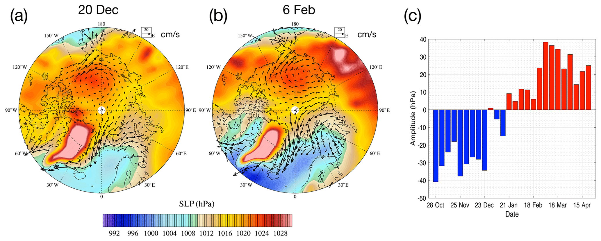
Figure 6Daily sea level pressure from the NYF dataset (filled contour) and modeled sea ice motion by TS045 (vectors) on 20 December (a) and 6 February (b). The wintertime Arctic oscillation (AO) index of the NYF dataset is in panel (c). See the text for detailed methods to compute the AO.
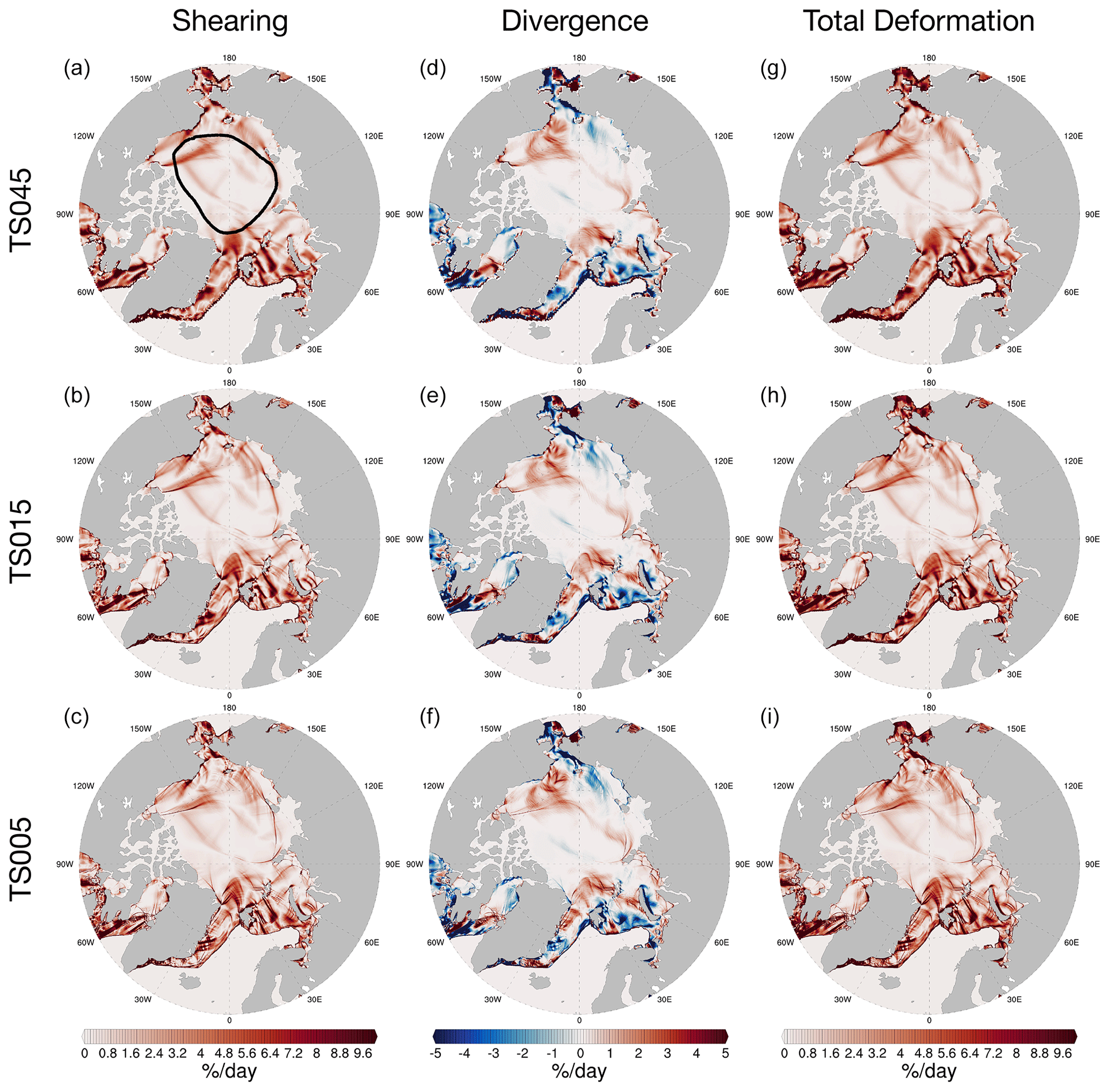
Figure 7Daily deformation fields on 20 December. The first, second, and third rows show the deformation fields for TS045, TS015, and TS005, respectively. Deformation rates include shearing rate (a–c), divergence rate (d–f), and total deformation rate (g–i). The region for further statistical analysis including spatial scaling is outlined in black in the first panel. All results are based on experiments with NDTE = 960.
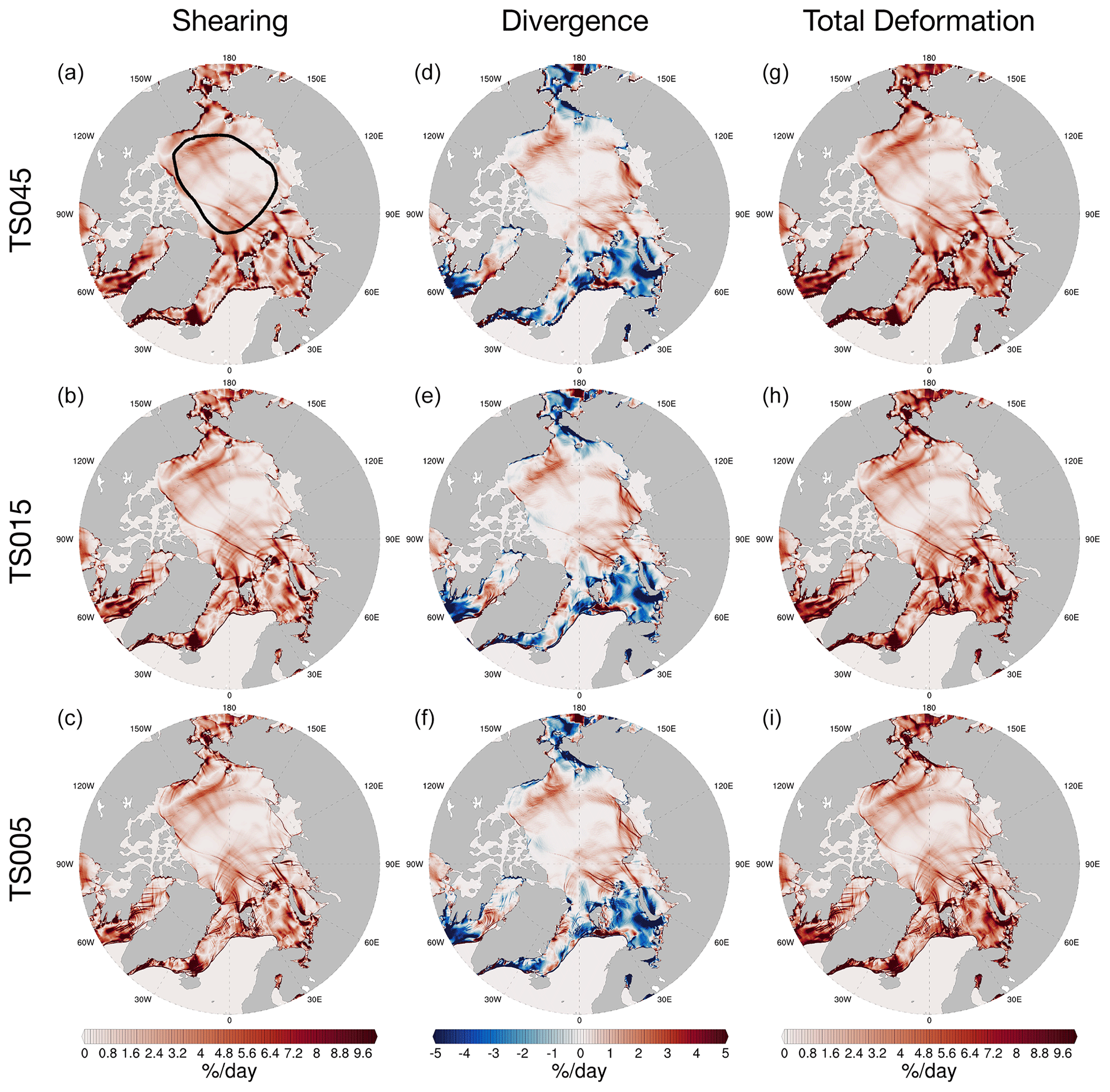
Figure 8Same as in Fig. 7, but for 6 February.
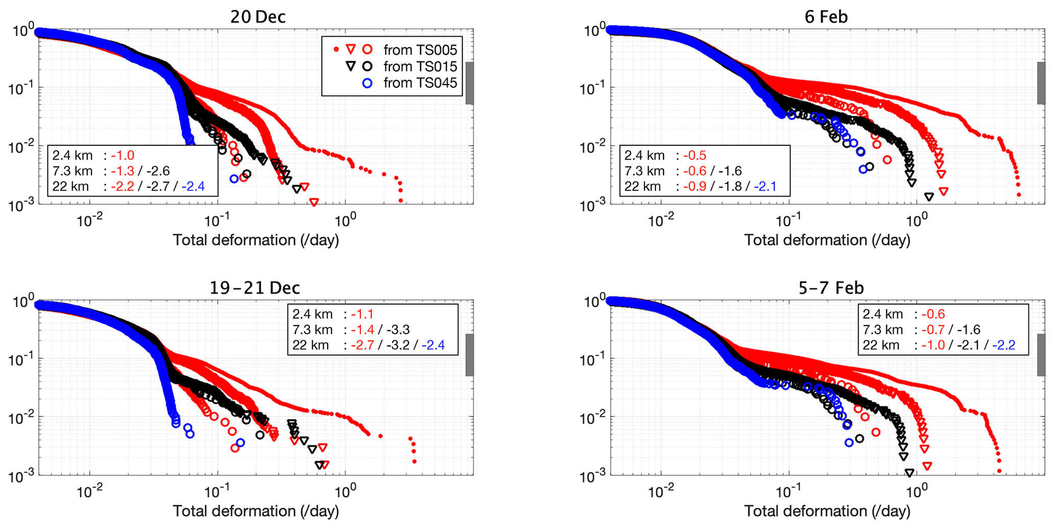
Figure 9Cumulative density functions for the total deformation rates on 20 December and 6 February. The region of study is outlined in Figs. 7 and 8. Daily rates are shown in the first row, and 3 d rates are in the second row. Colors indicate the cumulative PDFs from the model results from different grids (red: TS005; black: TS015; blue: TS045). With spatial coarsening of TS005, we compute the cumulative PDF at the spatial scales corresponding to the native resolution of TS015 and TS045. In turn, the spatial coarsening with TS015 is also applied to compute the cumulative PDFs at the equivalent resolution of TS045. The three spatial scales are marked by different shapes: 22 km (or TS045's native resolution) in circles; 7.3 km (or TS015's native resolution) in triangles; 2.4 km (or TS005's native resolution) in dots. Slopes are computed for the range of cumulated probability between 0.05 and 0.25 for all cumulative PDFs (marked out in grey in each panel), which correspond to the 95th and 75th percentile of the deformation fields, respectively. All results are based on experiments with NDTE = 960.
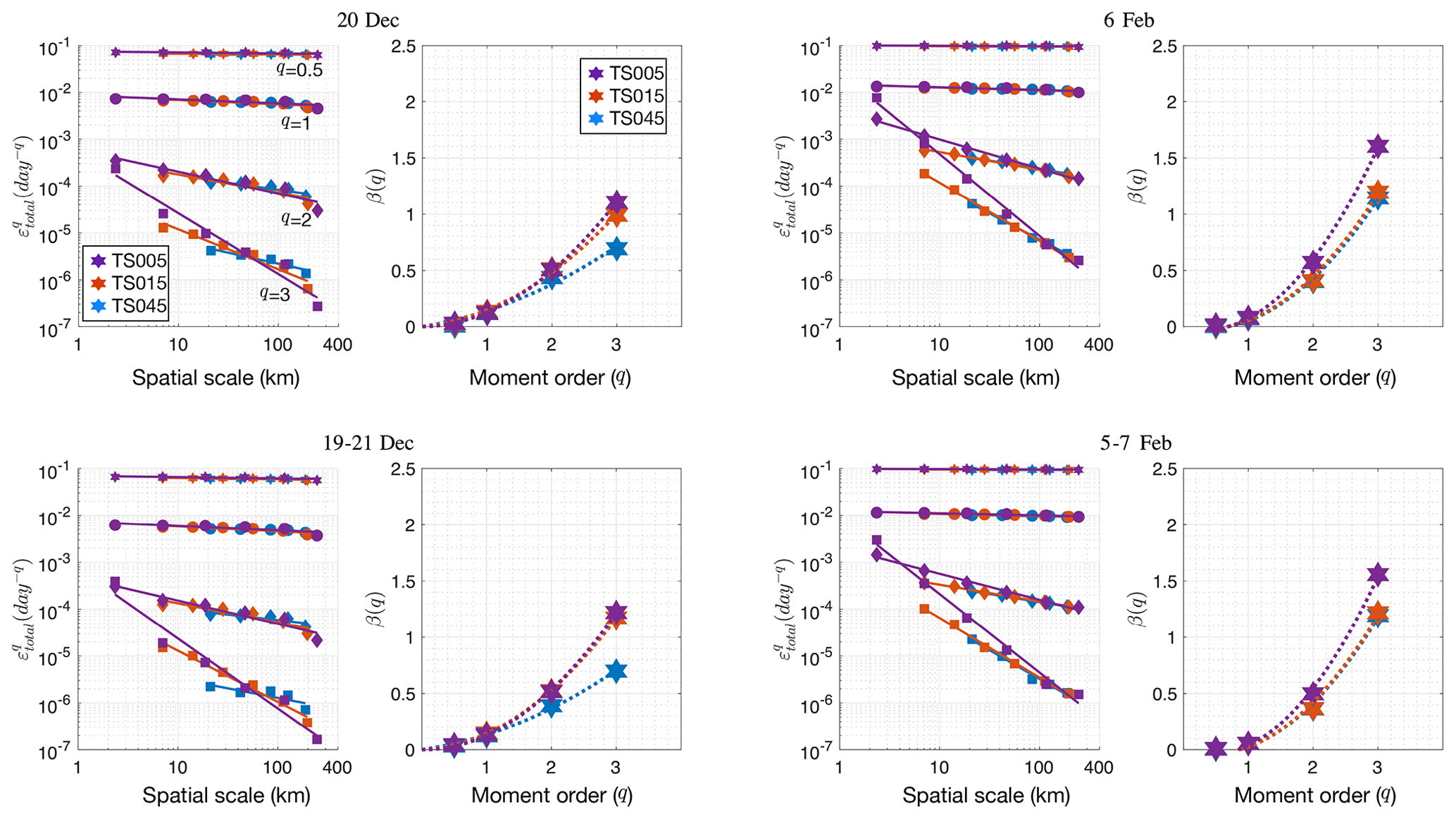
Figure 10Spatial scaling of total deformation rate for daily deformation fields (top row) and 3 d mean deformation fields (lower row). The daily mean velocity fields on 20 December and 6 February, as well as the 3 d mean velocity fields centering on 20 December and 6 February, are used to derive the scaling curves. Each panel contains the scaling curves and the structure function relating the scaling coefficients (β) to the moment of order (q). Similarly to Figs. 7, 8, and 9, the results are based on experiments with NDTE = 960. The detailed methodology used to compute the deformation rates with the model outputs is outlined in Appendix B.
3.3 Wintertime kinematics
We extend the analysis of spatial scaling to the winter months (December to February). Daily deformation fields are used to construct the time sequence of the spatial scaling exponent β for q=1 during this period (Fig. 11). The value of β shows very large day-to-day variability throughout the winter but is mostly within −0.1. During winter, the analyzed region (Fig. 7) mainly consists of packed ice, with the ice concentration close to 100 % and the mean ice thickness over 2 m (Fig. 5h). Similarly, as reported by Hutter et al. (2018), which is a model-based study, both packedness and thickness contribute to an exponent close to 0, and the central Arctic shows a very low scaling factor () in January. This is consistent with our result, which also shows β within 0.1. We do notice that in Hutter et al. (2018), hourly sea ice deformation fields are used to compute the scaling coefficients compared to daily fields in our current study. However, the spatial–temporal scaling in Hutter et al. (2018) shows very close values for β between hourly and daily results (their Fig. 7). We consider the low scaling coefficient produced by our model runs to be reasonable for characterizing sea ice kinematics in packed ice.
Furthermore, as revealed in Fig. 11, distinctive phases are present during the 3 months. During January, the exponent is between 0.02 and 0.03, which is lower (closer to 0) than the previous month of December (mainly between 0.04 and 0.06). The value of β also grows (more negative) towards February (around 0.04). There are several potential contributing factors to the differences in β. First, in order to ensure continuity at the beginning and end of the year, for December, the NYF dataset is based on interpolation of the years 1994 and 1995 of the NCEP reanalysis. Potentially, the atmospheric processes during this month may contain attenuated spatial and temporal variability. Second, in the NYF dataset, the dominant atmospheric variability (AO) shifts from negative in December to positive in January and February. This corresponds to the systematic shift of β during this period. However, a simple regression of AO on various scales (daily to weekly) yields no significant statistical correlation with β. Since the atmospheric forcing dominates large-scale sea ice drift, we conjecture that regarding atmospheric forcing, the fine-scale atmospheric processes (such as spatial and temporal wind variability) serve as the missing link between large-scale drift and small-scale kinematics and statistics. Lastly, the sea ice status, including sea ice strength and rheology, dominates the shearing as well as convergence and divergence failures at the local scale. The thickening of the sea ice throughout the winter months may also contribute to the increase in ice strength and the overall decrease in β.

Figure 11Spatial scaling exponents of the total deformation for q=1 for daily fields during winter. The region analyzed is outlined in the first panel in Fig. 7. Model output with the TS005 grid and NDTE = 960 is used for the analysis. The exponent sequence from daily fields (blue line, left y axis) is accompanied by its 14 d running mean (orange line, right y axis).
3.4 Numerical convergence of EVP
In this section we evaluate the sensitivity of the modeled sea ice kinematics to the EVP subcycling and asymptotic convergence. The elastic wave term introduced in the EVP is more effectively damped with more subcycles, leading to consistent deformation fields. This asymptotic convergence of the deformation fields to EVP subcycling is examined in this study. In Fig. 12 we show the probability density function (or PDF) of daily deformation rates during wintertime (December to February) for the three grids. All the simulations obtain a good shape for the tail of the PDF, approaching a slope of −3. For the total deformation rate, there is a well-defined mode at 0.1 % d−1 to 0.2 % d−1 for runs with NDTE = 960, and at NDTE = 120, there is a slight shift of the mode to higher values (between 0.5 % d−1 and 1 % d−1 for TS015 and TS005). At different resolutions, the EVP subcycling count plays a different role in the shape of the PDF. For TS045, the PDF is consistent between different subcycle counts. But for TS015 and TS005, there are much more evident differences: (1) with larger NDTE, there are more regions with smaller shearing and divergence (less than 0.1 % d−1); (2) there is general convergent behavior of the shape of the PDF when NDTE is large (e.g., NDTE >480 for TS015). This behavior also applies for specific days (see Figs. S2 and S3 for the PDF on 20 December and 6 February, respectively). The PDFs of high-resolution runs (TS015 and TS005) show better tail structure, and furthermore, the slopes are also better characterized (i.e., closer linear fittings at −3) with larger values of NDTE. For TS045, the tail of the PDF suffers from a lack of samples for large deformation events. This indicates that an insufficient EVP subcycle count leads to overall non-convergent deformation rate distributions.
A visual inspection of the deformation fields reveals the loss of kinematic features when convergence is not attained. Figure 13 shows the daily total deformation fields on 20 December as simulated with different NDTE values for each grid. The most remarkable difference is between the runs with NDTE = 120 and NDTE = 960 with the highest resolution (i.e., TS005). Although the linear kinematic features are well-defined with NDTE = 960, the deformation field is much noisier for the run with NDTE = 120, with only the larger features detectable. The noise level is at about 1 % d−1, which corresponds to the mode of the PDF in Fig. 12. With larger values of NDTE, the noise level decreases and the deformation rate around the linear kinematic features becomes smaller. As a result, a convergent PDF and linear feature maps are obtained. One exemplary region is the Canadian Arctic Archipelago (CAA), where landfast sea ice dominates during winter in the model run with NDTE = 960. For example, Fig. S4 shows that the 2-week mean sea ice velocity within the CAA is lower than m s−1 (Lemieux et al., 2015). The detailed total deformation rate field within the CAA for TS005 (third row of Fig. 13) is further shown in Fig. S5. The experiment with NDTE = 120 shows much higher and noisier sea ice deformation fields than that with NDTE = 960. Overall, the results show that with the traditional EVP implementation, with higher resolution, even more subcycles are needed to reach convergence for the simulated kinematics. This causes a further increase in simulation cost, given that the dynamics time step is already decreased in high-resolution runs due to the Courant–Friedrichs–Lewy (CFL) condition in processes such as advection (Table 2).
For TS045, although the PDFs of the deformation rates are similar among runs with different NDTE values, the deformation field is also slightly noisier in runs with NDTE = 120 and NDTE = 240 than with NDTE = 960. The region with the biggest difference is within the Canadian Arctic Archipelago. We further evaluate the effect of subcycling by carrying out experiments with NDTE = 240 and NDTE = 960 for TS045 further to year 45 (Fig. 4). We show the difference in March (September) sea ice thickness between the NDTE = 960 run and the NDTE = 240 run in year 45 in Fig. 14a (14b). Although there is only less than 1 % difference in the basin-scale ice volume between the two experiments, the sea ice is remarkably thinner in the CAA in the run with NDTE = 960.
The difference in ice thickness is year-round (i.e., in both September and March). Specifically, in the run with NDTE = 960, an ice arch forms by the eastern end of the Lancaster Sound and near Amund Ringnes Island, resulting in thicker ice in these regions. In other parts of the CAA, the ice is thinner by about 15 to 20 cm on average and up to 1 m thinner in certain areas. As shown in Fig. 14c, the run with NDTE = 240, which started from year 1, has already reached equilibrium in sea ice thickness and volume in the CAA well before year 35. However, in the run with NDTE = 960, which starts from year 35, the model status gradually shifts to another equilibrium status for ice thickness towards year 45. The overall volume difference is uniformly 100 km3 in March and September, which consists of about 6.5 % of the total volume in September. We further attribute the difference in winter ice thickness to the thermodynamic (Fig. 14d), advection (Fig. 14e), and dynamical ridging–rafting (Fig. 14f) contributions during the freeze-up seasons, computed as multiyear mean fields for December, January, and February (DJF) of years 41 to 45. Specifically, in the CICE model, the 3-month mean ice volume tendencies due to thermodynamic growth, ice advection, and ridging are computed from the model diagnostics for the ice volume budget at Eulerian grid points. Compared with the run with NDTE = 960, there are small deformation events in the CAA in the run with NDTE = 240, which are arguably due to non-convergent EVP solutions (see also Fig. 13 for comparisons of deformation fields). Therefore, there is more of an ice thickness increase in the run with NDTE = 240 due to these events (Fig. 14f). Also, since September ice is thinner in the run with NDTE = 960, it is intuitive that the winter thermodynamic ice growth should be higher for NDTE = 960. On the contrary, the thermodynamic ice thickness growth is in general lower in the run with NDTE = 960, except for regions with the biggest thickness decrease in September compared with the run with NDTE = 240 (Fig. 14d and b). This is mainly due to the fact that the thermodynamic ice growth is also closely tied to the kinematics processes. With noisier sea ice movement fields in the run with NDTE = 240, sea ice formation and growth are also promoted with very small deformation events, resulting in more thermodynamic growth in the run with NDTE = 240. Compared to ridging and rafting, sea ice advection is mainly responsible for redistributing the ice mass and thus plays a minor role for the overall ice volume in the CAA in our experiments (Fig. 14e).
The dependence of the modeled sea ice thickness in the CAA on EVP convergence in our study is purely numerical, but it calls for further attention from both modelers and modeling data users. It highlights the importance of the numerical convergence of EVP (or any other candidate solvers to VP) on the modeled sea ice climatology in fast ice regions. Since the experiments are idealized in this study, the effects in realistic simulations may also be subjected to grid resolution and staggering, as well as coupling and feedback processes.
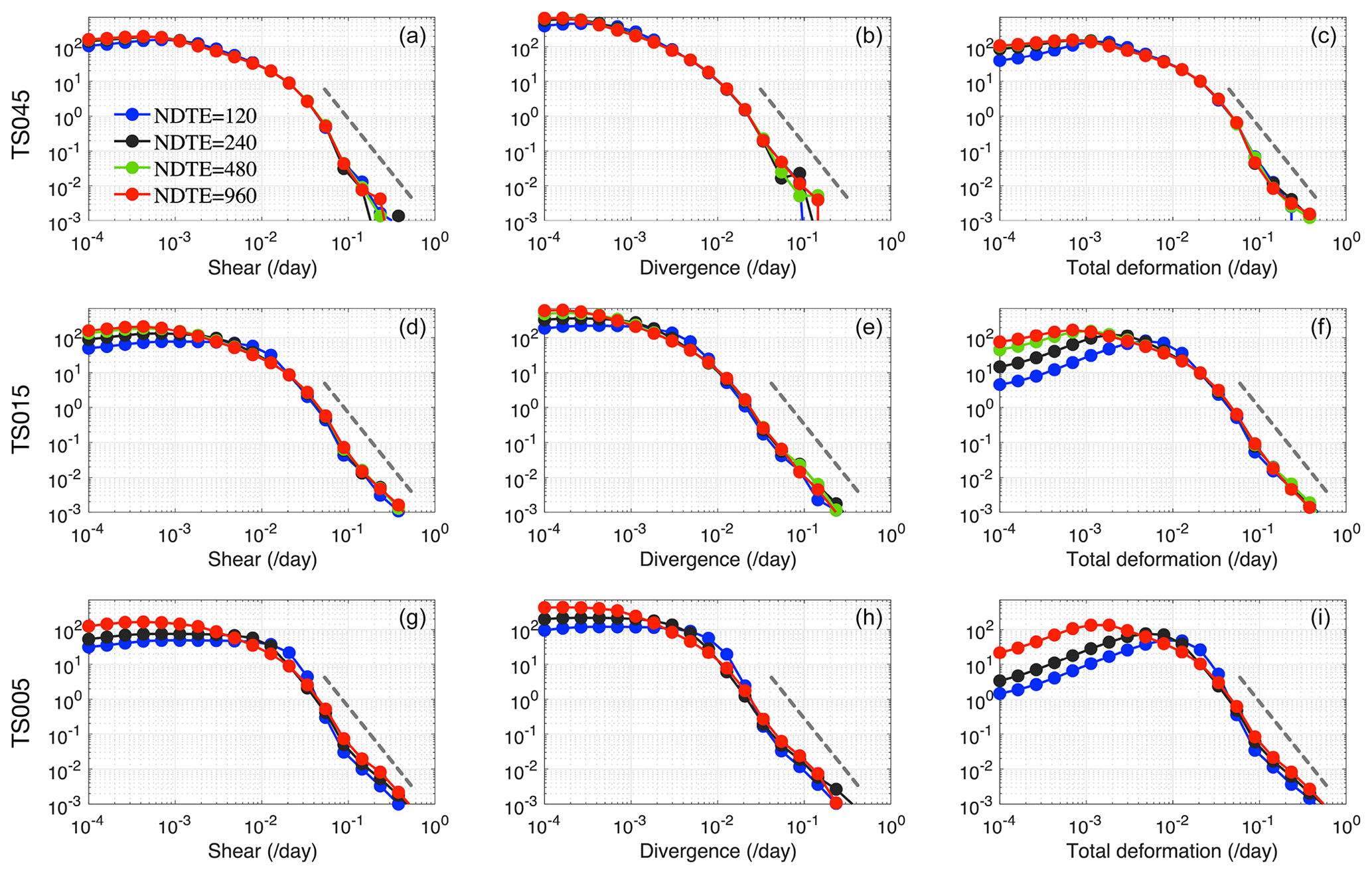
Figure 12Probability density of modeled daily deformation rates during winter months (December to February) with TS045 (first row), TS015 (second row), and TS005 (third row). The region of study is outlined in Fig. 7. The shearing rate (left column), divergence rate (central column), and total deformation rate (right column) are shown. Runs with different EVP configurations (NDTE from 120 to 960) are marked by the same color as in Fig. 4a. The theoretical slope for the PDF tail of −3 is shown in each panel for reference (grey dashed line).
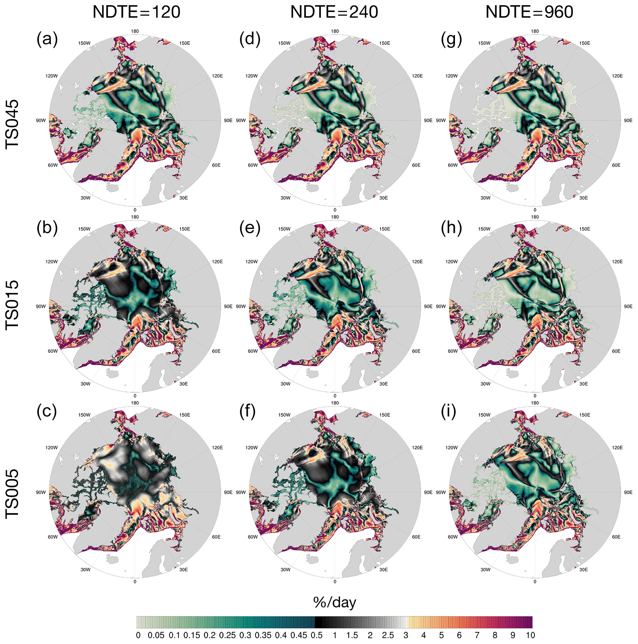
Figure 13Total deformation rate on 20 December with NDTE = 120 (a–c), 240 (d–f), and 960 (g–i). Each row represents a specific grid, including TS045 (a, d, g), TS015 (b, e, h), and TS005 (c, f, i). Results with NDTE = 960 are reproduced from Fig. 7. The color map is adjusted from Fig. 7 for increased resolution under 1 % d−1.
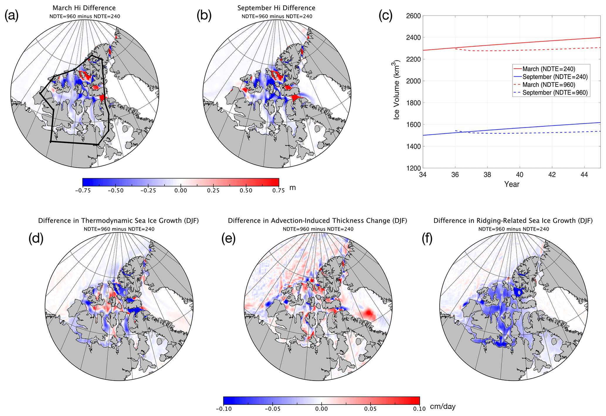
Figure 14March (a) and September (b) sea ice thickness difference between the run with NDTE = 240 and that with NDTE = 960 of year 50 for TS045 (NDTE = 960 minus NDTE = 240). Sea ice volume in March and September within the CAA (outlined in panel a) since year 41 is shown in panel (c). Differences in mean sea ice growth rate due to thermodynamics (d), advection (e), and dynamic ridging (f) during winter months (DJF) are computed for multiple winters (DJF of years 41 to 50). Blue (red) indicates lower (higher) ice growth during freeze-up in the run with NDTE = 960 than NDTE = 240 during winter.
In this paper we carried out sea ice simulations with a multi-resolution framework with the Community Earth System Model. A grid hierarchy is constructed with a resolution range spanning climate simulations (0.45∘) to sub-mesoscale modeling (0.05∘). At 0.05∘, the grid resolution in the Arctic region is approximately 2.45 km. The grid hierarchy is incorporated into CESM, and by using atmospherically forced experiments, we simulate and evaluate sea ice kinematics and scaling properties with a multi-resolution approach. We have found good consistency of the Arctic sea ice climatology and kinematics across the resolution range. As shown in the spatial scaling analysis on the representative days, the modeled sea ice deformation is characterized by multi-fractal scaling for all three grid resolutions. In our study, high-resolution (0.05∘) runs yield the most trustworthy kinematic features, and the multi-resolution simulations provide a unique approach for evaluating sea ice kinematics at lower resolutions. Furthermore, the convergence of the elastic–viscous–plastic rheology model is evaluated, which shows the significant impact of EVP convergence on kinematic statistics and landfast ice in the Canadian Arctic Archipelago. The framework for utilizing the grid hierarchy, including TS045, TS015, and TS005, provides an infrastructure for multi-resolution simulations for both the ocean and sea ice in the future. The three grids and the model integration are openly provided for public use for version 1.2.1 of CESM.
Sea ice kinematics have been the focus of the high-resolution sea ice modeling community in recent years. Based on synthetic-aperture radar (SAR) remote sensing such as ASAR and RADARSAT, kilometer-level or finer observations of sea ice drift and deformation are made possible and serve as the backbone for the validation of high-resolution sea ice simulations. Modeling studies with structured grids such as MITgcm (Spreen et al., 2017; Hutter et al., 2018) are similar to our study, although model specifics are different. Sea ice deformation and scaling can easily be derived with model output for spatial scaling, but Lagrangian-based diagnostics are required for the full analysis of temporal scaling. In our study, we mainly utilized model output for the study of spatial scaling properties in Sect. 3.2, with an initial study of 3 d mean drift fields. Specifically, we have observed time-varying scaling properties, and the scaling coefficient correlates with the leading mode of atmospheric forcing (i.e., Arctic oscillation). In a future work, a full exploration of AO and ice-condition-dependent scaling analysis is planned with the grid hierarchy and CESM. The scaling analysis remains an important tool for evaluating sea ice kinematics, but it may be insufficient for fully evaluating the sea ice deformation properties. Novel statistics based on linear kinematics features (LKFs) are proposed in recent studies, such as Hutter and Losch (2020) and Ringeisen et al. (2019). The utilization of a full suite of diagnostics in our modeling framework, including temporal–spatial scaling and LKF-based approaches, is an important direction for future work.
In this study, the NYF dataset of CORE-2 is utilized. This potentially compromises the comparability of the model results with satellite observations such as SAR-based sea ice kinematics (Kwok et al., 2008; Marsan et al., 2004). The interannual forcing dataset (IAF) of CORE-2 and the JRA-55 dataset used by the Ocean Model Intercomparison Project phase 2 (OMIP2) can be utilized for historical simulations with the proposed grids. Furthermore, comparison can be made with specific satellite observations such as RGPS (Kwok et al., 2008). Although with large-scale coarse atmospheric forcings such as CORE-2, sea ice models can produce multi-fractal sea ice deformation events, how these events are governed by multi-scale atmospheric processes remains unclear. With different atmospheric forcing datasets such as CORE-2 and JRA-55, we plan to carry out a comparative study by using higher versions of the coupled model (i.e., version 2 of CESM). The dynamical and thermodynamic feedback of sea ice deformation can also be studied with an atmosphere–sea ice coupled modeling framework, with a multi-resolution setting for both the atmospheric and the sea ice component model, as in CESM.
Sea ice rheology models are key to the simulation of sea ice dynamics and reproducing linear kinematic features. Together with other parameter schemes including sea ice strength (H79 in this study) and ridging, parameters of these schemes are utilized for tuning the models towards certain observations (Bouchat and Tremblay, 2017). Specifically, the sea ice strength parameter (P*) and eccentricity of the elliptic yield curve of EVP are found to be tunable parameters to improve the modeling of sea ice dynamics. During the tuning of the sea ice models, the aforementioned novel statistics can also be integrated to improve rheology models such as the yield curve shape (Ringeisen et al., 2019). In Girard et al. (2009), EVP is found to be unable to reproduce the observed distribution of the deformation rate in the RGPS dataset. Furthermore, this study confirms much better consistency with scaled deformation fields of the model output. Similarly, in our study, we argue that the model's output should be studied on a coarser scale, i.e., the model's effective resolution, instead of the grid's native resolution. Another issue with modeling sea ice at very high resolution (such as TS005) is prominent observed anisotropic characteristics. In order to explore this issue, anisotropic rheology models such as EAP (Tsamados et al., 2013) can be utilized for a comparative study with standard EVP (or VP) with a very high-resolution setting (1 to 2 km in the Arctic Basin). This is planned in our future work with the updated version of the sea ice component (version 5 of CICE) in CESM.
While EVP provides a numerically stable and easy-to-implement solver for the traditional VP model, the convergence of EVP solutions to a VP model is the focus of many recent efforts (Lemieux et al., 2012; Kimmritz et al., 2015; Koldunov et al., 2019). Based on a traditional implementation of EVP in our model, we have witnessed asymptotic converging behavior of sea ice kinematics fields with an increased EVP subcycle count. But this comes at a large computational overhead: at 960 subcycles per step for TS005, the simulation speed is halved compared with 240 subcycles per step, and over 50 % of the computational time is consumed in EVP, with less than 0.5 SYPD for 1920 processor cores. Ideally, an efficient and scalable implicit solver promises a more elegant and numerically sound solution to solving problem of VP models (Lemieux et al., 2010). Also, adaptive methods that complement the convergence and efficiency problems of a traditional EVP solver, such as in Kimmritz et al. (2015) and Koldunov et al. (2019), are considered in our future work for the integration of upgraded versions of the coupled or sea ice model.
In Sect. 3.4, we have shown that the mean states for ice thickness and volume can be systematically shifted due to the numerical behavior of an EVP solver. Since this issue is purely numerical, the uncertainty caused by it is different from other factors, such as the choice of the ice strength parameterization scheme. In our study, the region most sensitive is landfast ice in the CAA, where a significant decrease in ice volume is seen when solver convergence is attained with enough subcycle counts. Furthermore, more subcycling is required for higher resolution to reach convergence. Given the wide adoption of VP and EVP in climate models, using the model outputs for climate research and applications (such as the projection of shipping routes) could face potential compromises if the convergence issue is overlooked. Careful choices should be made, especially for configuring EVP at different resolutions (Kiss et al., 2020). Since the asymptotic behavior of sea ice kinematics with EVP subcycling is investigated in this study, the convergence of the VP solver needs a further formal definition for the strict intercomparison of multiple solvers in the future (Lemieux et al., 2012). In Koldunov et al. (2019) the authors also discovered a sensitivity of modeled ice thickness to EVP subcycling, but there was an increase in ice thickness with more EVP subcycles (their Fig. 2). Also, the region with the most significant thickness change is different in Koldunov et al. (2019), covering both regions in the CAA and north of CAA and Greenland. Compared to our study, the different behavior with EVP subcycling in Koldunov et al. (2019) may be due to differences in the numerical experiments and model physics, including grid resolutions and ice thickness distribution settings. Although both show a relationship of ice thickness to the rheology model, more analysis is needed for the attribution and explanation of the aforementioned differences. Tidal processes and interactions with sea ice are potentially important for the simulation of landfast ice (Lemieux et al., 2018). Since these processes are absent in our current model, we plan to include parameterization schemes that account for the their influence on sea ice kinematics in the future.
With the wide availability of high-performance computing utilities and progress in model developments, high-resolution and even multi-resolution simulations are becoming more common for the climate modeling community. While 1∘ models are still dominant in the Coupled Model Intercomparison Project (CMIP), high-resolution models are informative regarding potential model biases and parameterization improvements. For example, three resolutions (1, 0.25, and 0.1∘) are built into the ACCESS-OM model for ocean–sea ice coupled simulations (Kiss et al., 2020). In the most recent ocean–sea ice model of the Geophysical Fluid Dynamics Laboratory (GFDL) (OM4.0; Adcroft et al., 2019), two resolutions are adopted: OM4p5 (0.5∘) and OM4p25 (0.25∘). Parameterization schemes in the ocean and the sea ice models are chosen and tuned to each specific resolution. For example, a mesoscale eddy-induced mixing parameterization is usually adopted for low-resolution ocean models (0.5∘ or coarser) but is inactive for higher resolutions. In our study, we use three resolutions for the study of Arctic sea ice kinematics: 0.45, 0.15, and 0.05∘. As is shown in the scaling analysis, this multi-resolution framework enables a comparative analysis across resolutions. Given that the modeled sea ice climatology is reasonable and consistent among the three resolutions, we consider the results adequate for the analysis of kinematics and scaling based on the coupling to the slab ocean model. Beyond the lower computational overhead of this approach, we can also attain an equilibrium status for the sea ice with fewer model years. Especially for the 0.05∘ grid (TS005), the computational cost and the duration is prohibitively high to fully spin up the ocean–sea ice coupled model. Furthermore, it reduces the uncertainty of ocean modeling on the sea ice, including (1) ocean model parameterization schemes that are not aligned and potentially not well-tuned between the different resolutions and (2) the avoidance of ocean and ocean–sea ice coupled internal variability that may potentially compromise comparability across the resolutions. For future work, a long-term, interannually forced simulation of the coupled ocean–sea ice system is planned under the multi-resolution framework and the spin-up strategy as adopted in this study. Specifically, a comparison with coinciding satellite observations can be carried out, such as the RGPS dataset.
The construction of the orthogonal grid in the northern patch (NP, as in Sect. 2) involves a numerical process of two steps. First, a series of embedding ellipses is constructed on the stereographic projection of NP from the North Pole (Fig. A1a). The outermost ellipse is a circle defined by the boundary between NP and SP. The innermost ellipse is a direct line that crosses the North Pole and links the two grid poles, which are prescribed locations on land. A smooth transition from the circle to the innermost ellipse is achieved by controlling the semi-major axes (a) and semi-minor axes (b) of the ellipses. Without the loss of generality, we rescale the projected NP so that the outermost ellipse is the unit circle and the innermost ellipse resides on the x axis; the layout is shown in Fig. A1a. Therefore, we have (1) for the outermost ellipse and (2) for the innermost ellipse a=α and b=0, where α is half of the distance between the two grid poles. To ensure a continued change in meridional grid scales on the NP–SP boundary, the change in b should be equal to that in a on the outermost ellipse. In Fig. A1b we show a possible relationship between a and b: , where . The slope of the curve can be computed to equal 1 when a (or b) approaches 1, ensuring the same change speed in a and b as well as a smooth meridional-scale transition on the NP–SP boundary. The ellipses, including a, b, and center locations, can then be determined according to these configurations and the required resolution. In this paper, we have chosen the following parameters for TS grids: the NP–SP boundary (ϕ) at about 10∘ N and the two poles at 63∘ N, 104∘ W and 59.5∘ N, 76∘ E, which are 180∘ apart but at different latitudes (red squares in Fig. A1a).
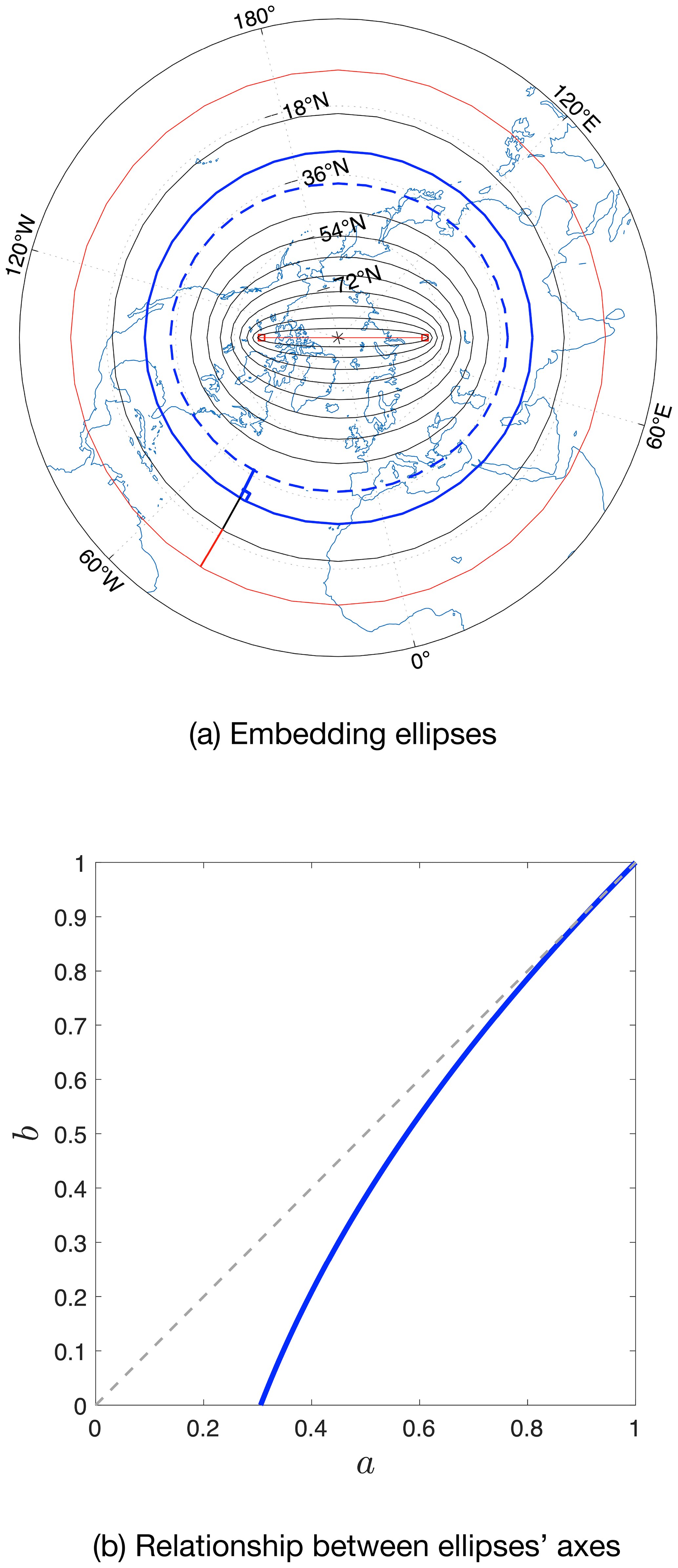
Figure A1Construction of the embedding ellipses and the orthogonal grid. In panel (a), we show in red the outermost ellipse (a circle) and the innermost ellipse (the direct link between the two grid poles marked by a red square). The numerical process of constructing an orthogonal grid is carried out between two adjacent ellipses, starting with points on the outermost ellipse and moving recursively down to the innermost one. The construction of a single step on the current ellipse (blue) to the next ellipse (dashed blue) is shown in panel (a). In panel (b), we show the relationship between the major axis and minor axis of the ellipses under a quadratic form (see Sect. A for details).
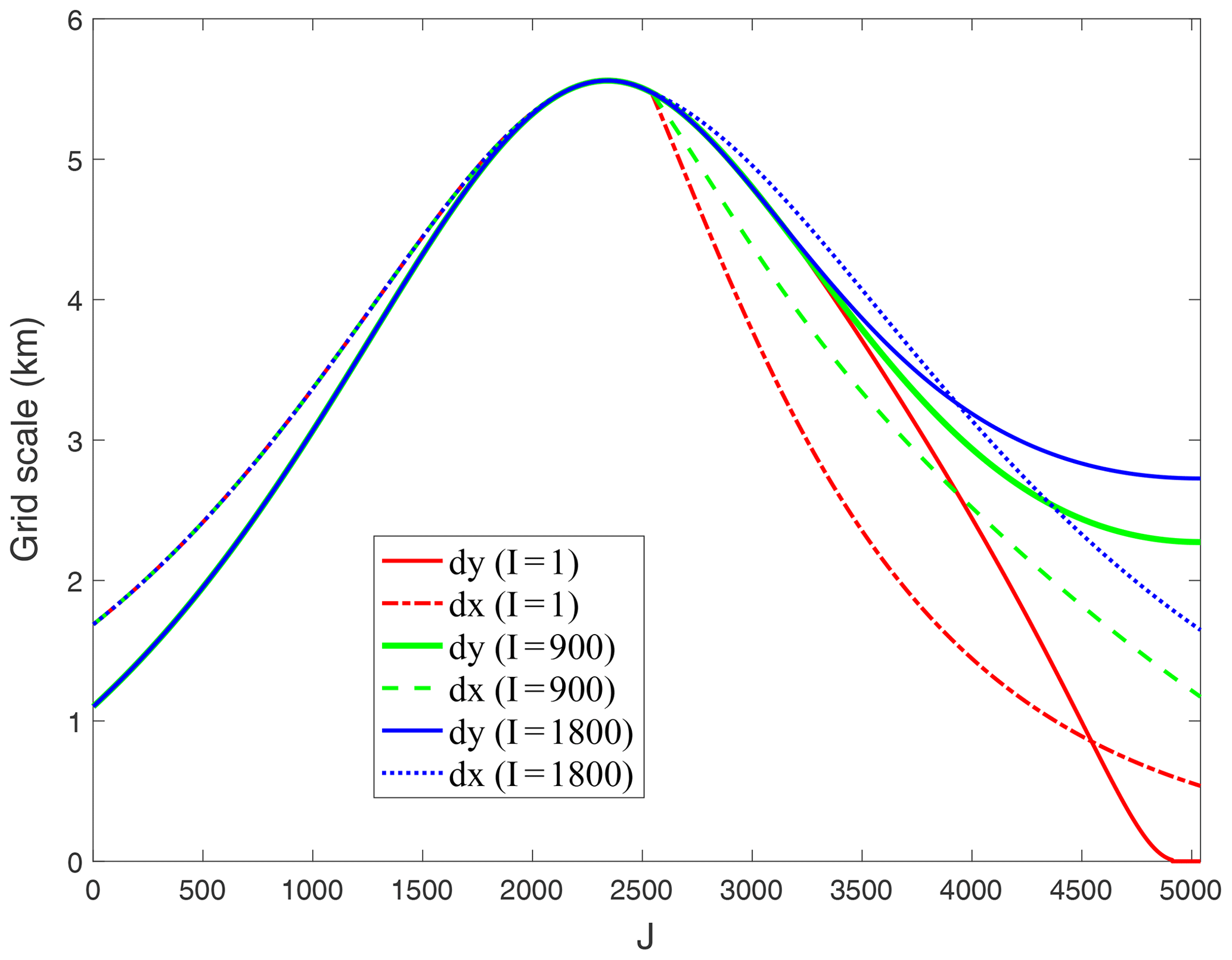
Figure A2Grid sizes along the “meridional” grid lines for TS005 (I and J dimensions are 7200 and 5040). Three typical lines are chosen: I=1, I=900 (1∕8 in the I direction), and I=1800 (1∕4 in the I direction). Grid sizes in both the I and J directions retain continued changes. The corresponding grid lines are also shown in Fig. 2 with the same color coding. Note that when I=1, dy (meridional grid size) approaches zero when J is close to the northern end (J=5400), which does not affect the model's time stepping since it is near the grid pole that resides on land.
Second, with the embedded ellipses, the orthogonal grid can be constructed from the outermost circle. Since NP is directly linked to SP at latitude ϕ, we specify the grid points on this boundary (i.e., the outermost circle) and extend into NP to form the meridional grid lines. The construction process is iterative; it starts from these points on the outermost ellipse and for each step constructs lines between two adjacent ellipses. In each step, the ending locations of the lines are located on the inner ellipse under orthogonality constraints. Figure A1a shows a specific example between two adjacent ellipses (marked by blue and dashed blue). This whole approach is similar to grid generation methods that are based on numerical integration processes, as in Madec and Imbard (1996) and Xu et al. (2015).
Figure A2 shows the meridional and zonal grid scales (dx and dy) along typical meridional grid lines for TS005. As shown, there is smooth transition of the meridional grid scale on the boundary of SP and NP (at about J=2520 for TS005). Also, the overall grid-scale anisotropy is kept lower than 1.5 in the oceanic areas.
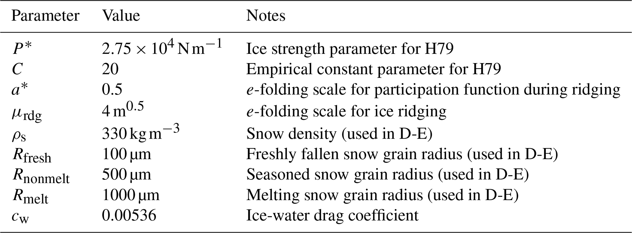
CICE (version 4.0) is the sea ice component of CESM (version 1.2.1). CICE is a full thermodynamic–dynamic model for sea ice, and with the coupling framework in CESM, CICE is forced with NCEP CORE-2 atmospheric forcings and coupled to the slab ocean model. Sea ice thickness distribution with five categories is adopted in our experiments, which is also the default configuration for CICE in CESM. In the vertical direction, we use four ice layers and one snow layer. The sea ice dynamics mainly include four components: (1) an elastic–viscous–plastic rheology model with an elliptic yield curve and the aspect ratio of 2 (Hunke and Dukowicz, 1997); (2) the ice strength model in Hibler (1979), referred to as H79, in which the ice strength is related to the mean ice thickness; (3) the ice ridging scheme as in Lipscomb et al. (2007); and (4) the advection scheme of transport remapping (Dukowicz and Baumgardner, 2000). Specifically, in Ungermann et al. (2017) H79 is found to produce a more reasonable basin-wide sea ice thickness distribution than Rothrock (1975), and this is also confirmed in our earlier study comparing the two ice strength schemes. For thermodynamics, the delta–Eddington (D-E) radiation scheme is adopted, with explicit melt-pond formulation (Briegleb and Light, 2007). The atmospheric and oceanic stress on sea ice is parameterized as follows. For the atmosphere, the boundary layer process is carried out to determine the flux exchanges and wind stresses, following the coupling routine in CESM. For oceanic drag, the stress is parameterized with the coefficient cw and dependent on ice–ocean drift speed differences. Key parameters of CICE in our experiments are shown in Table B1.
Table B1Key model parameters of CICE in numerical experiments.
With Arakawa-B grid staggering in CICE, we carry out the spatial scaling analysis of sea ice drift fields according to Marsan et al. (2004). A exemplary case with nine local grid cells is shown in Fig. C1. To compute a specific spatial derivate (i.e., ), the line integral is computed to calculate the flux through the boundary of the specified area (Eq. C2). The deformation rates can be computed according to Eqs. (1) through (3). For the area from i1 to i2 and j1 to j2, the line integral consists of the flux computation over the eastern (i=i2), western (), northern (j=j2), and southern () boundaries. The spatial scale is defined as the square root of the integrated cell areas.
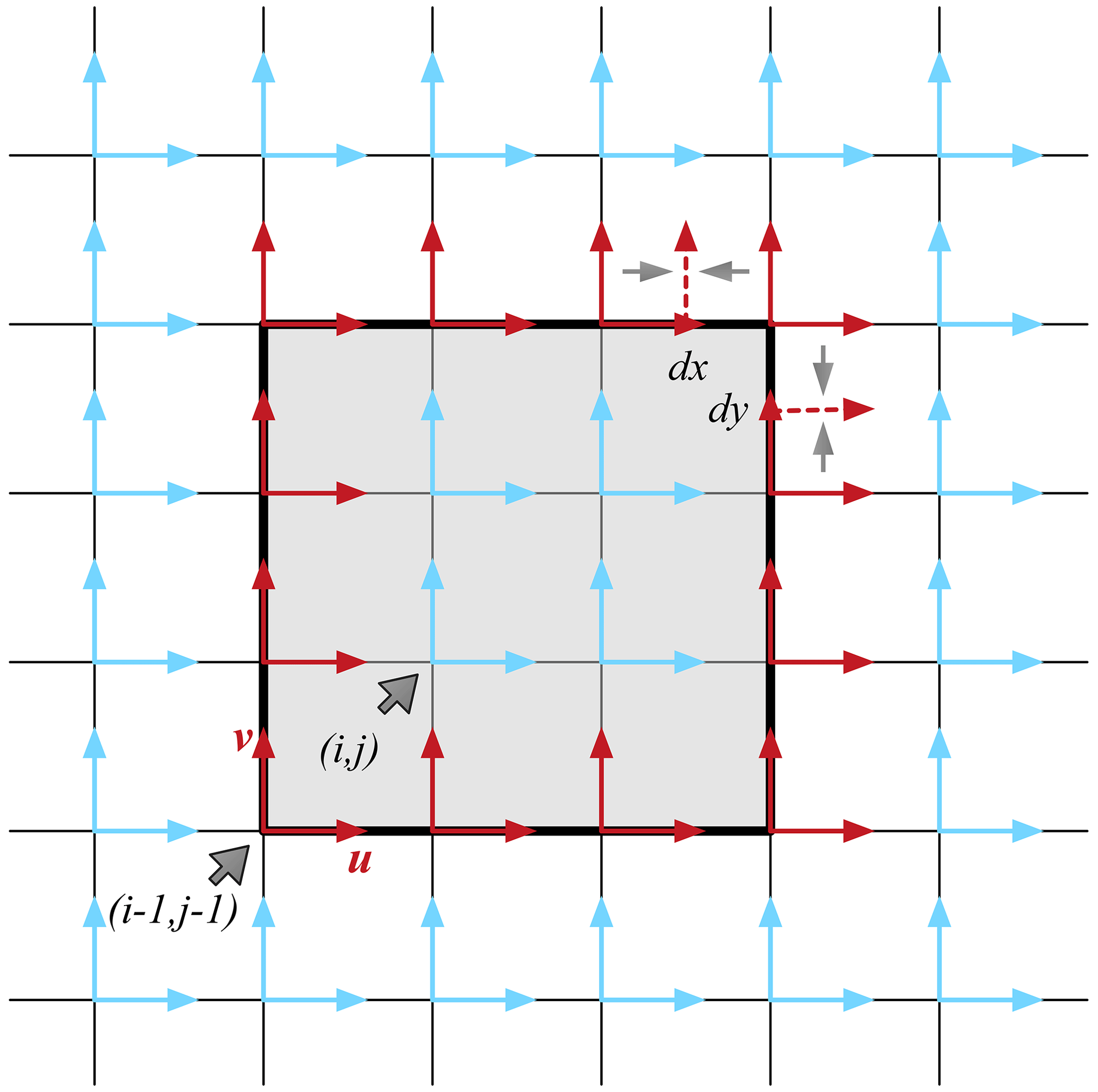
Figure C1Example for spatial scaling analysis with a local area of 9 (i.e., 3×3) model cells. The horizontal (or vertical) direction is in the model's eastern (or northern) direction, indexed by discrete indices of i (or j). The sea ice drift velocities that are used to compute the line integral for and are marked in red. For contrast, other velocities are marked in blue. Since velocities are defined in the top right corner of each cell, they are interpolated on the cell edges to compute the integral. The interpolated velocities are marked by dashed vectors corresponding to the averaging operation in Eq. (C2).
The three grids in this article (TS045, TS015, and TS005) are openly provided in the binary grid format of POP and CICE. Modifications to CESM (version 1.2.1) are made to incorporate the new grids, with model configurations of CICE and coupling with the atmospheric forcing dataset (T62). Auxiliary datasets are also provided, including (1) coupling interpolators of TS grids to T62 and (2) CICE monthly history files during March. The grids and model integration are also available for the Community Integrated Earth System Model (CIESM; Lin et al., 2020). All the code and data are hosted at https://doi.org/10.5281/zenodo.3842282 (Xu et al., 2020).
CESM code and ESMF regridding utility are available for download at http://cesm.ucar.edu (last access: 20 February 2020) and https://www.earthsystemcog.org/projects/esmf/regridding (last access: 12 March 2020).
The supplement related to this article is available online at: https://doi.org/10.5194/gmd-14-603-2021-supplement.
SX designed the grid generation algorithm and carried out grid generation. SX and JM carried out model integration of TS grids in CESM and the numerical experiments. SX, LZ, JM, and YZ analyzed the model outputs. All the authors contributed to the writing of the paper.
The authors declare that they have no conflict of interest.
The authors would like to thank the editors and referees for their invaluable efforts to improve the paper. This work is partially supported by the National Key R & D Program of China (no. 2017YFA0603902), the General Program of National Science Foundation of China (no. 42030602), and the Tsinghua University Initiative Scientific Research Program (no. 2019Z07L01001). This work is also partially supported by the Center for High-Performance Computing and System Simulation, Pilot National Laboratory for Marine Science and Technology (Qingdao). The authors would also like to thank the National Supercomputing Center at Wuxi for the computational and technical support during the numerical experiments.
The authors gratefully acknowledge the CESM development team at NCAR and the user community of CESM for providing the open-source usage of CESM and its component models, as well as their valuable help. We would also like to express sincere thanks for the use of ESMF utilities during the integration of TS grids in CESM.
This research has been supported by the National Key R & D Program of China (grant no. 2017YFA0603902), the General Program of National Science Foundation of China (grant no. 42030602), and the Tsinghua University Initiative Scientific Research Program (grant no. 2019Z07L01001).
This paper was edited by Alexander Robel and reviewed by Frederic Dupont, Véronique Dansereau, and Nils Hutter.
Adcroft, A., Anderson, W., Balaji, V., Blanton, C., Bushuk, M., Dufour, C. O., Dunne, J. P., Griffies, S. M., Hallberg, R., Harrison, M. J., Held, I. M., Jansen, M. F., John, J. G., Krasting, J. P., Langenhorst, A. R., Legg, S., Liang, Z., McHugh, C., Radhakrishnan, A., Reichl, B. G., Rosati, T., Samuels, B. L., Shao, A., Stouffer, R., Winton, M., Wittenberg, A. T., Xiang, B., Zadeh, N., and Zhang, R.: The GFDL Global Ocean and Sea Ice Model OM4.0: Model Description and Simulation Features, J. Adv. Model. Earth Syst., 11, 3167–3211, https://doi.org/10.1029/2019MS001726, 2019. a
Bouchat, A. and Tremblay, B.: Using sea-ice deformation fields to constrain the mechanical strength parameters of geophysical sea ice, J. Geophys. Res.-Oceans, 122, 5802–5825, https://doi.org/10.1002/2017JC013020, 2017. a
Briegleb, B. P. and Light, B.: A Delta-Eddington Multiple Scattering Parameterization for Solar Radiation in the Sea Ice Component of the Community Climate System Model (No. NCAR/TN-472+STR), Tech. rep., University Corporation for Atmospheric Research, https://doi.org/10.5065/D6B27S71, 2007. a
Chelton, D. B., deSzoeke, R. A., Schlax, M. G., El Naggar, K., and Siwertz, N.: Geographical Variability of the First Baroclinic Rossby Radius of Deformation, J. Phys. Oceanogr., 28, 433–460, https://doi.org/10.1175/1520-0485(1998)028<0433:GVOTFB>2.0.CO;2, 1998. a
Dansereau, V., Weiss, J., Saramito, P., and Lattes, P.: A Maxwell elasto-brittle rheology for sea ice modelling, The Cryosphere, 10, 1339–1359, https://doi.org/10.5194/tc-10-1339-2016, 2016. a
Dukowicz, J. K. and Baumgardner, J. R.: Incremental Remapping as a Transport/Advection Algorithm, J. Comput. Phys., 160, 318–335, https://doi.org/10.1006/jcph.2000.6465, 2000. a, b
Dupont, F., Higginson, S., Bourdallé-Badie, R., Lu, Y., Roy, F., Smith, G. C., Lemieux, J.-F., Garric, G., and Davidson, F.: A high-resolution ocean and sea-ice modelling system for the Arctic and North Atlantic oceans, Geosci. Model Dev., 8, 1577–1594, https://doi.org/10.5194/gmd-8-1577-2015, 2015. a
ETOPO1: Global Relief Model, National Centers for Environmental Information, https://doi.org/10.7289/V5C8276M, 2019. a
Girard, L., Weiss, J., Molines, J. M., Barnier, B., and Bouillon, S.: Evaluation of high-resolution sea ice models on the basis of statistical and scaling properties of Arctic sea ice drift and deformation, J. Geophys. Res.-Oceans, 114, C08015, https://doi.org/10.1029/2008JC005182, 2009. a
Girard, L., Bouillon, S., Weiss, J., Amitrano, D., Fichefet, T., and Legat, V.: A new modeling framework for sea-ice mechanics based on elasto-brittle rheology, Ann. Glaciol., 52, 123–132, https://doi.org/10.3189/172756411795931499, 2011. a
Griffies, S. M., Danabasoglu, G., Durack, P. J., Adcroft, A. J., Balaji, V., Böning, C. W., Chassignet, E. P., Curchitser, E., Deshayes, J., Drange, H., Fox-Kemper, B., Gleckler, P. J., Gregory, J. M., Haak, H., Hallberg, R. W., Heimbach, P., Hewitt, H. T., Holland, D. M., Ilyina, T., Jungclaus, J. H., Komuro, Y., Krasting, J. P., Large, W. G., Marsland, S. J., Masina, S., McDougall, T. J., Nurser, A. J. G., Orr, J. C., Pirani, A., Qiao, F., Stouffer, R. J., Taylor, K. E., Treguier, A. M., Tsujino, H., Uotila, P., Valdivieso, M., Wang, Q., Winton, M., and Yeager, S. G.: OMIP contribution to CMIP6: experimental and diagnostic protocol for the physical component of the Ocean Model Intercomparison Project, Geosci. Model Dev., 9, 3231–3296, https://doi.org/10.5194/gmd-9-3231-2016, 2016. a
Hallberg, R.: Using a resolution function to regulate parameterizations of oceanic mesoscale eddy effects, Ocean Modell., 72, 92–103, https://doi.org/10.1016/j.ocemod.2013.08.007, 2013. a
Hibler, W. D.: A Dynamic Thermodynamic Sea Ice Model, J. Phys. Oceanogr., 9, 815–846, https://doi.org/10.1175/1520-0485(1979)009<0815:ADTSIM>2.0.CO;2, 1979. a, b, c, d
Hunke, E. C. and Dukowicz, J. K.: An Elastic-Viscous-Plastic Model for Sea Ice Dynamics, J. Phys. Oceanogr., 27, 1849–1867, https://doi.org/10.1175/1520-0485(1997)027<1849:AEVPMF>2.0.CO;2, 1997. a, b, c
Hunke, E. C. and Lipscomb, W. H.: CICE: the Los Alamos Sea Ice Model Documentation and Software User's Manual Version 4.0 LA-CC-06-012, Tech. rep., Los Alamos National Laboratory, Los Alamos, NM 87545, USA, 2008. a
Hutter, N. and Losch, M.: Feature-based comparison of sea ice deformation in lead-permitting sea ice simulations, The Cryosphere, 14, 93–113, https://doi.org/10.5194/tc-14-93-2020, 2020. a, b
Hutter, N., Losch, M., and Menemenlis, D.: Scaling properties of Arctic sea ice deformation in a high-resolution viscous-plastic sea ice model and in satellite observations, J. Geophys. Res.-Oceans, 123, 672–687, https://doi.org/10.1002/2017JC013119, 2018. a, b, c, d, e, f, g
Jahn, A., Sterling, K., Holland, M. M., Kay, J. E., Maslanik, J. A., Bitz, C. M., Bailey, D. A., Stroeve, J., Hunke, E. C., Lipscomb, W. H., and Pollak, D. A.: Late-Twentieth-Century Simulation of Arctic Sea Ice and Ocean Properties in the CCSM4, J. Climate, 25, 1431–1452, https://doi.org/10.1175/JCLI-D-11-00201.1, 2012. a
Kimmritz, M., Danilov, S., and Losch, M.: On the convergence of the modified elastic-viscous-plastic method for solving the sea ice momentum equation, J. Comput. Phys., 296, 90–100, https://doi.org/10.1016/j.jcp.2015.04.051, 2015. a, b
Kiss, A. E., Hogg, A. McC., Hannah, N., Boeira Dias, F., Brassington, G. B., Chamberlain, M. A., Chapman, C., Dobrohotoff, P., Domingues, C. M., Duran, E. R., England, M. H., Fiedler, R., Griffies, S. M., Heerdegen, A., Heil, P., Holmes, R. M., Klocker, A., Marsland, S. J., Morrison, A. K., Munroe, J., Nikurashin, M., Oke, P. R., Pilo, G. S., Richet, O., Savita, A., Spence, P., Stewart, K. D., Ward, M. L., Wu, F., and Zhang, X.: ACCESS-OM2 v1.0: a global ocean–sea ice model at three resolutions, Geosci. Model Dev., 13, 401–442, https://doi.org/10.5194/gmd-13-401-2020, 2020. a, b
Koldunov, N. V., Danilov, S., Sidorenko, D., Hutter, N., Losch, M., Goessling, H., Rakowsky, N., Scholz, P., Sein, D., Wang, Q., and Jung, T.: Fast EVP Solutions in a High-Resolution Sea Ice Model, J. Adv. Model. Earth Syst., 11, 1269–1284, https://doi.org/10.1029/2018MS001485, 2019. a, b, c, d, e, f, g
Kwok, R., Hunke, E. C., Maslowski, W., Menemenlis, D., and Zhang, J.: Variability of sea ice simulations assessed with RGPS kinematics, J. Geophys. Res., 113, C11012, https://doi.org/10.1029/2008JC004783, 2008. a, b, c
Lemieux, J.-F., Tremblay, B., Sedlác̆ek, J., Tupper, P., Thomas, S., Huard, D., and Auclair, J.-P.: Improving the numerical convergence of viscous-plastic sea ice models with the Jacobian-free Newton-Krylov method, J. Comput. Phys., 229, 2840–2852, https://doi.org/10.1016/j.jcp.2009.12.011, 2010. a, b
Lemieux, J.-F., Knoll, D. A., Tremblay, B., Holland, D. M., and Losch, M.: A comparison of the Jacobian-free Newton-Krylov method and the EVP model for solving the sea ice momentum equation with a viscous-plastic formulation: A serial algorithm study, J. Comput. Phys., 231, 5926–5944, https://doi.org/10.1016/j.jcp.2012.05.024, 2012. a, b, c
Lemieux, J.-F., Tremblay, L. B., Dupont, F., Plante, M., Smith, G. C., and Dumont, D.: A basal stress parameterization for modeling landfast ice, J. Geophys. Res.-Oceans, 120, 3157–3173, https://doi.org/10.1002/2014JC010678, 2015. a
Lemieux, J.-F., Lei, J., Dupont, F., Roy, F., Losch, M., Lique, C., and Laliberté, F.: The Impact of Tides on Simulated Landfast Ice in a Pan-Arctic Ice-Ocean Model, J. Geophys. Res.-Oceans, 123, 7747–7762, https://doi.org/10.1029/2018JC014080, 2018. a
Lin, Y., Huang, X., Liang, Y., Qin, Y., Xu, S., Huang, W., Xu, F., Liu, L., Wang, Y., Peng, Y., Wang, L., Xue, W., Fu, H., Zhang, G. J., Wang, B., Li, R., Zhang, C., Lu, H., Yang, K., Luo, Y., Bai, Y., Song, Z., Wang, M., Zhao, W., Zhang, F., Xu, J., Zhao, X., Lu, C., Chen, Y., Luo, Y., Hu, Y., Tang, Q., Chen, D., Yang, G., and Gong, P.: Community Integrated Earth System Model (CIESM): description and evaluation, J. Adv. Model. Earth Syst., 12, e2019MS002036, https://doi.org/10.1029/2019MS002036, 2020. a
Lipscomb, W. H., Hunke, E. C., Maslowski, W., and Jakacki, J.: Improving ridging schemes for high-resolution sea ice models, J. Geophys. Res.-Oceans, 112, C03S91, https://doi.org/10.1029/2005JC003355, 2007. a, b
Locarnini, R. A., Mishonov, A. V., Antonov, J. I., Boyer, T. P., Garcia, H. E., Baranova, O. K., Zweng, M. M., Paver, C. R., Reagan, J. R., Johnson, D. R., Hamilton, M., and Seidov, D.: NOAA Atlas NESDIS 73 World Ocean Atlas 2013, Volume 1: Temperature, 1315 East-West Highway Silver Spring, MD 20910-3282, USA, 2013. a
Madec, G. and Imbard, M.: A global ocean mesh to overcome the North Pole singularity, Clim. Dynam., 12, 381–388, https://doi.org/10.1007/BF00211684, 1996. a, b
Marsan, D., Stern, H., Lindsay, R., and Weiss, J.: Scale Dependence and Localization of the Deformation of Arctic Sea Ice, Phys. Rev. Lett., 93, 178501, https://doi.org/10.1103/PhysRevLett.93.178501, 2004. a, b, c, d, e, f, g, h
Murray, R. J.: Explicit Generation of Orthogonal Grids for Ocean Models, J. Comput. Phys., 126, 251–273, https://doi.org/10.1006/jcph.1996.0136, 1996. a
Rampal, P., Weiss, J., Marsan, D., Lindsay, R., and Stern, H.: Scaling properties of sea ice deformation from buoy dispersion analysis, J. Geophys. Res., 113, C03002, https://doi.org/10.1029/2007JC004143, 2008. a
Rampal, P., Dansereau, V., Olason, E., Bouillon, S., Williams, T., Korosov, A., and Samaké, A.: On the multi-fractal scaling properties of sea ice deformation, The Cryosphere, 13, 2457–2474, https://doi.org/10.5194/tc-13-2457-2019, 2019. a, b, c
Rigor, I. G., Wallace, J. M., and Colony, R. L.: Response of Sea Ice to the Arctic Oscillation, J. Climate, 15, 2648–2663, https://doi.org/10.1175/1520-0442(2002)015<2648:ROSITT>2.0.CO;2, 2002. a
Ringeisen, D., Losch, M., Tremblay, L. B., and Hutter, N.: Simulating intersection angles between conjugate faults in sea ice with different viscous–plastic rheologies, The Cryosphere, 13, 1167–1186, https://doi.org/10.5194/tc-13-1167-2019, 2019. a, b
Rothrock, D. A.: The energetics of the plastic deformation of pack ice by ridging, J. Geophys. Res., 80, 4514–4519, https://doi.org/10.1029/JC080i033p04514, 1975. a
Scholz, P., Sidorenko, D., Gurses, O., Danilov, S., Koldunov, N., Wang, Q., Sein, D., Smolentseva, M., Rakowsky, N., and Jung, T.: Assessment of the Finite-volumE Sea ice-Ocean Model (FESOM2.0) – Part 1: Description of selected key model elements and comparison to its predecessor version, Geosci. Model Dev., 12, 4875–4899, https://doi.org/10.5194/gmd-12-4875-2019, 2019. a
Schweiger, A., Lindsay, R., Zhang, J., Steele, M., Stern, H., and Kwok, R.: Uncertainty in modeled Arctic sea ice volume, J. Geophys. Res.-Oceans, 116, C00D06, https://doi.org/10.1029/2011JC007084, 2011. a
Spreen, G., Kwok, R., Menemenlis, D., and Nguyen, A. T.: Sea-ice deformation in a coupled ocean–sea-ice model and in satellite remote sensing data, The Cryosphere, 11, 1553–1573, https://doi.org/10.5194/tc-11-1553-2017, 2017. a
Tsamados, M., Feltham, D. L., and Wilchinsky, A. V.: Impact of a new anisotropic rheology on simulations of Arctic sea ice, J. Geophys. Res.-Oceans, 118, 91–107, https://doi.org/10.1029/2012JC007990, 2013. a, b
Ungermann, M., Tremblay, L. B., Martin, T., and Losch, M.: Impact of the ice strength formulation on the performance of a sea ice thickness distribution model in the Arctic, J. Geophys. Res.-Oceans, 122, 2090–2107, https://doi.org/10.1002/2016JC012128, 2017. a
Wang, Q., Wekerle, C., Danilov, S., Wang, X., and Jung, T.: A 4.5 km resolution Arctic Ocean simulation with the global multi-resolution model FESOM 1.4, Geosci. Model Dev., 11, 1229–1255, https://doi.org/10.5194/gmd-11-1229-2018, 2018. a
Weiss, J. and Dansereau, V.: Linking scales in sea ice mechanics, Phil. Trans. R. Soc. A, 375, 20150352, https://doi.org/10.1098/rsta.2015.0352, 2017. a
Xu, S., Song, M., Liu, J., Wang, B., Li, L., Huang, W., Liu, L., Xia, K., Xue, W., Pu, Y., Dong, L., Shen, S., Hu, N., Liu, M., and Sun, W.: Simulation of sea ice in FGOALS-g2: Climatology and late 20th century changes, Adv. Atmos. Sci., 30, 658–673, https://doi.org/10.1007/s00376-013-2158-4, 2013. a
Xu, S., Wang, B., and Liu, J.: On the use of Schwarz–Christoffel conformal mappings to the grid generation for global ocean models, Geosci. Model Dev., 8, 3471–3485, https://doi.org/10.5194/gmd-8-3471-2015, 2015. a
Xu, S., Ma, J., Zhou, L., Zhang, Y., Wang, B., and Liu, J.: Multi-scale sea ice kinematics modeling dataset with a tripolar grid hierarchy (TS grids) in CESM [Data set], Zenodo, https://doi.org/10.5281/zenodo.3842282, 2020. a
Zweng, M., Reagan, J., Antonov, J., Locarnini, R., Mishonov, A., Boyer, T., Garcia, H., Baranova, O., Johnson, D., Seidov, D., and Biddle, M.: NOAA Atlas NESDIS 74 WORLD OCEAN ATLAS 2013, Volume 2: Salinity, 1315 East-West Highway Silver Spring, MD 20910-3282, USA, 2013. a
- Abstract
- Introduction
- Grid generation and model integration
- Experiments and analysis
- Summary and discussion
- Appendix A: Orthogonal grid for northern patch
- Appendix B: Sea ice model (CICE) configuration and parameters
- Appendix C: Scaling analysis for kinematics
- Code and data availability
- Author contributions
- Competing interests
- Acknowledgements
- Financial support
- Review statement
- References
- Supplement