Harmonized Emissions Component (HEMCO) 3.0 as a versatile emissions component for atmospheric models: application in the GEOS-Chem, NASA GEOS, WRF-GC, CESM2, NOAA GEFS-Aerosol, and NOAA UFS models

Emissions are a central component of atmospheric chemistry models. The Harmonized Emissions Component (HEMCO) is a software component for computing emissions from a user-selected ensemble of emission inventories and algorithms. It allows users to re-grid, combine, overwrite, subset, and scale emissions from different inventories through a configuration file and with no change to the model source code. The configuration file also maps emissions to model species with appropriate units. HEMCO can operate in offline stand-alone mode, but more importantly it provides an online facility for models to compute emissions at runtime. HEMCO complies with the Earth System Modeling Framework (ESMF) for portability across models. We present a new version here, HEMCO 3.0, that features an improved three-layer architecture to facilitate implementation into any atmospheric model and improved capability for calculating emissions at any model resolution including multiscale and unstructured grids. The three-layer architecture of HEMCO 3.0 includes (1) the Data Input Layer that reads the configuration file and accesses the HEMCO library of emission inventories and other environmental data, (2) the HEMCO Core that computes emissions on the user-selected HEMCO grid, and (3) the Model Interface Layer that re-grids (if needed) and serves the data to the atmospheric model and also serves model data to the HEMCO Core for computing emissions dependent on model state (such as from dust or vegetation). The HEMCO Core is common to the implementation in all models, while the Data Input Layer and the Model Interface Layer are adaptable to the model environment. Default versions of the Data Input Layer and Model Interface Layer enable straightforward implementation of HEMCO in any simple model architecture, and options are available to disable features such as re-gridding that may be done by independent couplers in more complex architectures. The HEMCO library of emission inventories and algorithms is continuously enriched through user contributions so that new inventories can be immediately shared across models. HEMCO can also serve as a general data broker for models to process input data not only for emissions but for any gridded environmental datasets. We describe existing implementations of HEMCO 3.0 in (1) the GEOS-Chem “Classic” chemical transport model with shared-memory infrastructure, (2) the high-performance GEOS-Chem (GCHP) model with distributed-memory architecture, (3) the NASA GEOS Earth System Model (GEOS ESM), (4) the Weather Research and Forecasting model with GEOS-Chem (WRF-GC), (5) the Community Earth System Model Version 2 (CESM2), and (6) the NOAA Global Ensemble Forecast System – Aerosols (GEFS-Aerosols), as well as the planned implementation in the NOAA Unified Forecast System (UFS). Implementation of HEMCO in CESM2 contributes to the Multi-Scale Infrastructure for Chemistry and Aerosols (MUSICA) by providing a common emissions infrastructure to support different simulations of atmospheric chemistry across scales.

1 Introduction

Emissions are a crucial component in modeling atmospheric chemistry. Models apply emission fluxes calculated from inputs including gridded inventory data, point source data, and environmental data. These data originate from an ensemble of sources with different spatiotemporal resolution and extent, covering different chemical species. They may need to be re-gridded, combined, overlaid, scaled, or extended through computational algorithms to produce the model emissions. Here we present the Harmonized Emission Component (HEMCO) 3.0 as a versatile tool to ingest and process emission data in atmospheric models and share these data across models.

Emissions can be computed in atmospheric models either offline or online. An offline emissions module precomputes emissions on the target model grid and archives them as time-varying files for input to the model. An online emissions module computes emissions at runtime within the model from a set of input files containing emission information and with rules for how this information is to be used. Offline processing of emissions is used by many models, such as the PREP-CHEM-SRC preprocessor system (Freitas et al., 2011) in the WRF-Chem model (Grell et al., 2005; Fast et al., 2006) and the Sparse Matrix Operator Kernel Emissions system (SMOKE, https://www.cmascenter.org/smoke/, last access: 2 September 2021) in the CMAQ (Byun and Schere, 2006) and CAMx (Ramboll Environment and Health, 2020) models. The advantage of computing emissions at the preprocessing stage is the versatility in preprocessing tools and low computational requirements at runtime. However, the preprocessing of emissions is a cumbersome step and the resulting emission files may be prohibitively large (Jähn et al., 2020). Any change to the emissions requires re-running the preprocessor code. Emissions dependent on environmental variables computed in the atmospheric model cannot be treated offline, complicating the infrastructure.

The Harmonized Emissions Component (HEMCO), originally developed by Keller et al. (2014) and formerly called the Harvard–NASA Emissions Component, computes emissions customized to user needs through a configuration file and a database library. Atmospheric chemistry modelers can use HEMCO either offline in a stand-alone mode to compute and archive emissions or online to compute emissions at runtime and serve them to the model at each time step. HEMCO can select, modify, re-grid, combine, and supersede emission inventories and algorithms without changing the model source code. Built-in algorithms called “extensions” compute emissions dependent on environmental data and model state variables such as for vegetation, dust, lightning, and oceans. Subgrid processing of emissions to account for fast chemistry, as in ship plumes (Vinken et al., 2011), is also done in extensions. Selection of HEMCO extensions is done in the configuration file and the computations are done independently of the atmospheric model, allowing for immediate portability to other models.

HEMCO was originally developed for the GEOS-Chem atmospheric chemistry model (Bey et al., 2001; Eastham et al., 2018), wherein the current version HEMCO 2.0 has two different implementations. The “Classic” version of GEOS-Chem with single-node shared-memory parallelization (OpenMP) and rectilinear latitude–longitude grids (Bey et al., 2001) uses HEMCO to its full extent including reading, re-gridding, and temporal interpolation of input files. In GEOS-Chem Classic, HEMCO is used not only for emissions but as a general data broker to read and process all model input data, including meteorological fields and initial conditions. This has enabled in particular the FlexGrid algorithm to run GEOS-Chem on any custom nest selected at runtime (Li et al., 2021). This implementation of HEMCO is also used in the recently developed coupling of GEOS-Chem with the Weather Research and Forecasting (WRF) model (WRF-GC; Lin et al., 2020; Feng et al., 2021).

The “High-Performance” version of GEOS-Chem (GCHP; Eastham et al., 2018) uses a different implementation of HEMCO 2.0. GCHP is designed for multi-node massively parallel computation using a distributed-memory parallelization (MPI) enabled by the NASA Model Analysis and Prediction Layer (MAPL; Suarez et al., 2007), which acts as the model's infrastructure and handles inter-node communication. MAPL is built upon the Earth System Modeling Framework (ESMF, Hill et al., 2004) and handles data read, re-gridding, and interpolation, so the corresponding HEMCO routines are disabled. This implementation of HEMCO is also presently used by the GOCART aerosol model operating within the MAPL-based NASA Goddard Earth Observing System (GEOS) Earth science model (Rienecker et al., 2008; Randles et al., 2017).

HEMCO 2.0 has several limitations that limit its portability to other models. First, the re-gridding capability is limited to latitude–longitude grids. Second, its implementation in distributed-memory environments uses MAPL-specific features. Third, it has a multiplicity of model access points that introduce unnecessary dependency on model code. Fourth, it requires that emissions be computed on the model grid, which may introduce inaccuracies in masking of regional inventories and in nonlinear computations, and further necessitates duplicate copies of HEMCO to handle different resolutions in multiscale model applications such as WRF-GC.

HEMCO 3.0 overcomes all these limitations of HEMCO 2.0. Construction of HEMCO 3.0 was motivated by interest from the Community Earth System Model Version 2 (CESM2; Pfister et al., 2020) and the NOAA Unified Forecast System (UFS; Campbell et al., 2020) in using HEMCO as an emissions component. This led us to develop a more modularized and powerful structure to increase accuracy and portability to different atmospheric models including with multiscale and unstructured grids. HEMCO 3.0 preserves a shared common core for calculating emissions by selecting, adding, superseding (masking), and scaling emission inventories as specified by the user. Other parts of HEMCO are modularized to facilitate the incorporation of HEMCO into the specific software environment of the target model. A three-layer architecture is created to separate (1) input and re-gridding of data, (2) emission calculations using the HEMCO Core, and (3) coupling to the target model, including export of the computed emissions and import of model state variables for state-dependent emissions (extensions). With this new modularity and flexibility, HEMCO can be readily implemented in a wide range of model environments. Use of a common HEMCO Core facilitates the sharing of emission data and algorithms between models and the intercomparisons of model results.

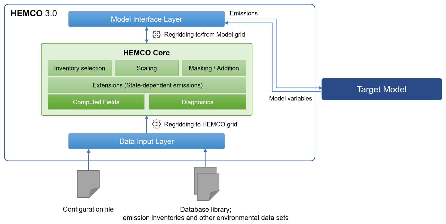
Figure 1 Three-layer architecture of HEMCO 3.0 including the Data Input Layer, the HEMCO Core, and the Model Interface Layer.

2 HEMCO 3.0 description

2.1 General architecture

HEMCO 3.0 is modularized into a three-layer architecture as shown in Fig. 1, consisting of the Data Input Layer, the HEMCO Core, and the Model Interface Layer. The Data Input Layer reads the configuration file and the database library of emission inventories and other environmental information, and it re-grids the data to a user-defined HEMCO grid (finer than or identical to the model grid). The HEMCO Core assembles the emissions on the basis of instructions in the configuration file including adding, scaling, and masking of individual inventories, as well as computing emissions dependent on model state variables and environmental data (through algorithms referred to as HEMCO extensions). The Model Interface Layer communicates HEMCO output (including emission fluxes, diagnostics, and other computed data) to the target atmospheric model (hereafter referred to as “the model”), with re-gridding to the model grid if needed, and takes in and re-grids model variables to the HEMCO grid for use in HEMCO extensions. The Data Input Layer and the Model Interface Layer have different implementations depending on the architecture of the model. The HEMCO Core, where emissions are computed, is the same in all cases. HEMCO operates on a horizontal “HEMCO grid” that may be any user-desired grid configuration (e.g., finer than the model grid or the finest element of a multiscale model grid), with the other layers handling the re-gridding to and from the HEMCO grid as necessary. 2-D (horizontal) emissions can be released at the surface or allocated vertically on the model grid as specified by the user through the HEMCO configuration file. 3-D emission databases (such as for aircraft emissions) are re-gridded vertically to the model grid through the Data Input Layer.

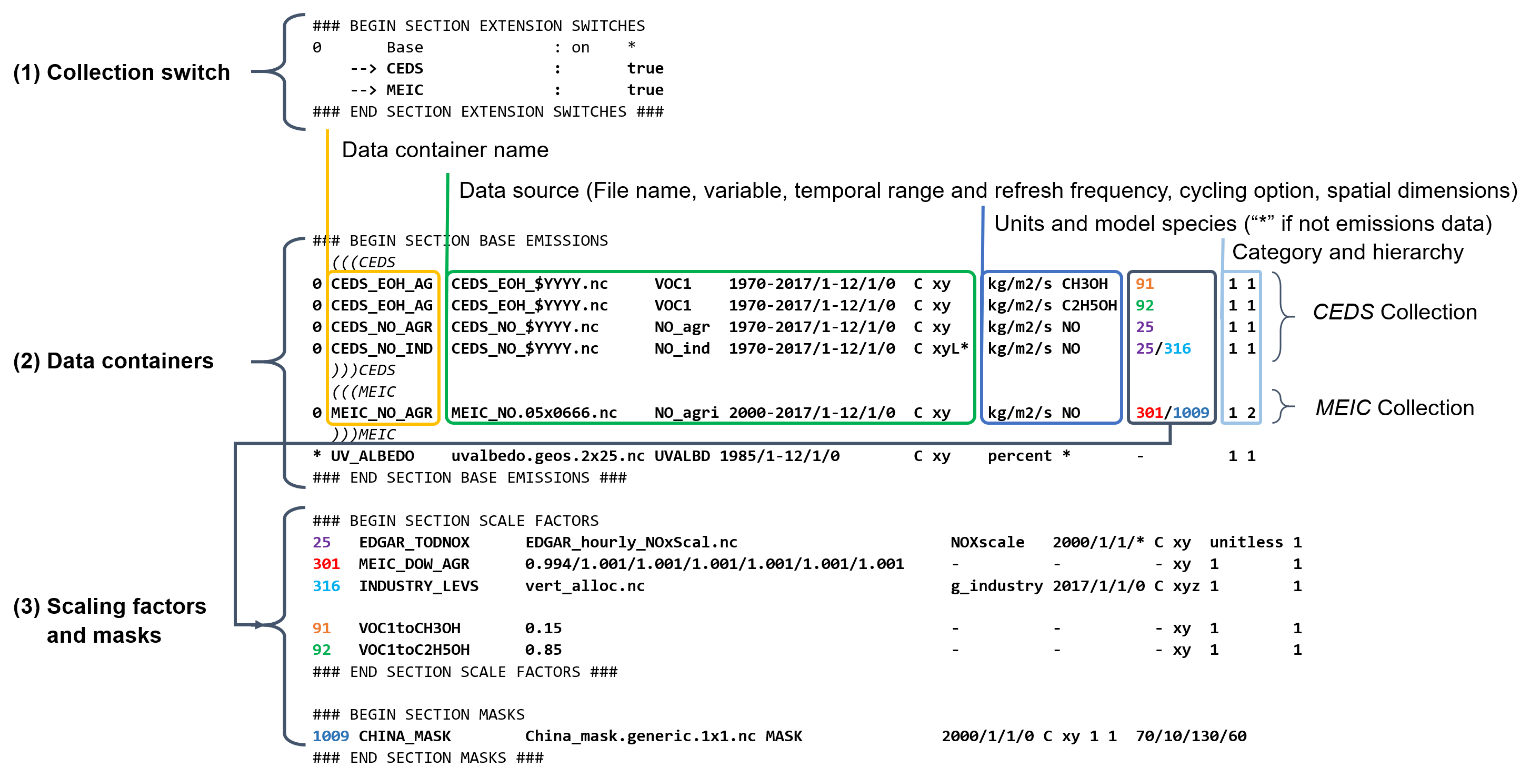
Figure 2 Sample HEMCO configuration file. The HEMCO configuration file is organized in three sections: (1) switches for “collections” of data containers, (2) data containers to be used in the model simulation optionally organized into “collections”, and (3) scaling and masking rules to be used. Entries are organized in a similar format, including a number and/or name, the data source (NetCDF file and variable name, numbers, or mathematical expressions), the temporal range and spatial dimensions, and their category and hierarchy (in the same category, data entries with higher hierarchy take precedence). For data containers, scaling factors and masks are applied by referencing the numbered scaling factor and mask entries (colored text).

The HEMCO configuration file (example in Fig. 2) controls the operation of all HEMCO layers, fully describing the relationship between the input data read by the Data Input Layer, the processing by the HEMCO Core, and the data passed to the model by the Model Interface Layer. It is organized as individual entries for data, scaling factors, and masks. Each entry is numbered or named and includes information about the source of data (usually a NetCDF file name but may be a number or mathematical expression in simple cases). For NetCDF data files, each entry specifies the NetCDF variable name to be read (allowing the mapping from NetCDF input species to model species), the temporal range, refresh frequency, cycling option (whether to continuously cycle the data or require an exact date match), and spatial dimension (2-D or 3-D data, with the option to specify a custom vertical distribution for 2-D data). Also included is the model species name, the scaling factors to be applied, and the hierarchy (priority order used for masking). If a data entry does not include a species name, the entry is treated as generic data and is read into HEMCO, scaled, masked, and made available to the model upon request. Entries may be organized in the form of “collections” enabled or disabled in bulk using switches. HEMCO comes with a default database library of emission inventories and environmental datasets that is updated with every new GEOS-Chem version release, but users can readily add their own by processing the data into COARDS-compliant NetCDF format and providing the corresponding configuration file entries. A detailed HEMCO user guide is available on the GEOS-Chem Wiki (http://wiki.seas.harvard.edu/geos-chem/index.php/The_HEMCO_User%27s_Guide, last access: 7 January 2021).

The HEMCO configuration file makes it possible for different models with different chemical species to share a single set of emissions input data (the “HEMCO database library”) without manually preprocessing the files for each mechanism. The variable name option in each entry allows for the mapping of the species name in the NetCDF file to the model species name. One can also partition a class of species from the inventory into individual model species. For example, total alcohols in the CEDS inventory (Hoesly et al., 2018) are to be emitted as 15 % methanol and 85 % ethanol in the CAM-chem model (Emmons et al., 2020). In that example, as illustrated in Fig. 2, HEMCO scaling factors are used to scale the same input variable by 15 % and 85 % into the CH3OH and C2H5OH model species. The scaling factor functionality in HEMCO can be used for temporal scaling (diurnal, day-of-week, seasonal, interannual) or to convert units from the emission inventory in the HEMCO database library to the target model. For example, emissions may be provided as kilograms of NO_x on an NO₂ mass basis in the inventory file but emitted as NO and NO₂ in the model. Scaling factors can be specified for each individual entry in the HEMCO configuration file, allowing different scaling factors to be applied for different inventories, sectors, and species. HEMCO accepts scaling factors as constant numbers, temporally explicit (diurnal, day-of-week, seasonal, interannual) numbers, or as a gridded NetCDF data file.

The Data Input Layer processes each enabled entry in the HEMCO configuration file, reads the corresponding files from disk, and re-grids them to the HEMCO grid. The Data Input Layer then passes the data to the HEMCO Core in the form of data containers corresponding to each entry in the configuration file.

2.2 HEMCO Core

The HEMCO Core calculates emissions with summations, masks, and scaling factors specified in the HEMCO configuration file. It includes Fortran modules that define the HEMCO state, HEMCO data types (e.g., configuration options, date and time, chemical species and their physical properties, file containers storing input data, and data containers storing data processed by HEMCO), and the driver routine that computes emissions and stores them in data containers. All data types are contained in a variable called the HEMCO state (HcoState) and passed as an argument to all HEMCO subroutines in the code. This allows multiple instances of HEMCO to operate simultaneously, as multiple copies of HEMCO state can co-exist independently. The HEMCO Core also includes an error handling and logging component.

Table 1 Emission inventories currently in the default HEMCO 3.0 library.

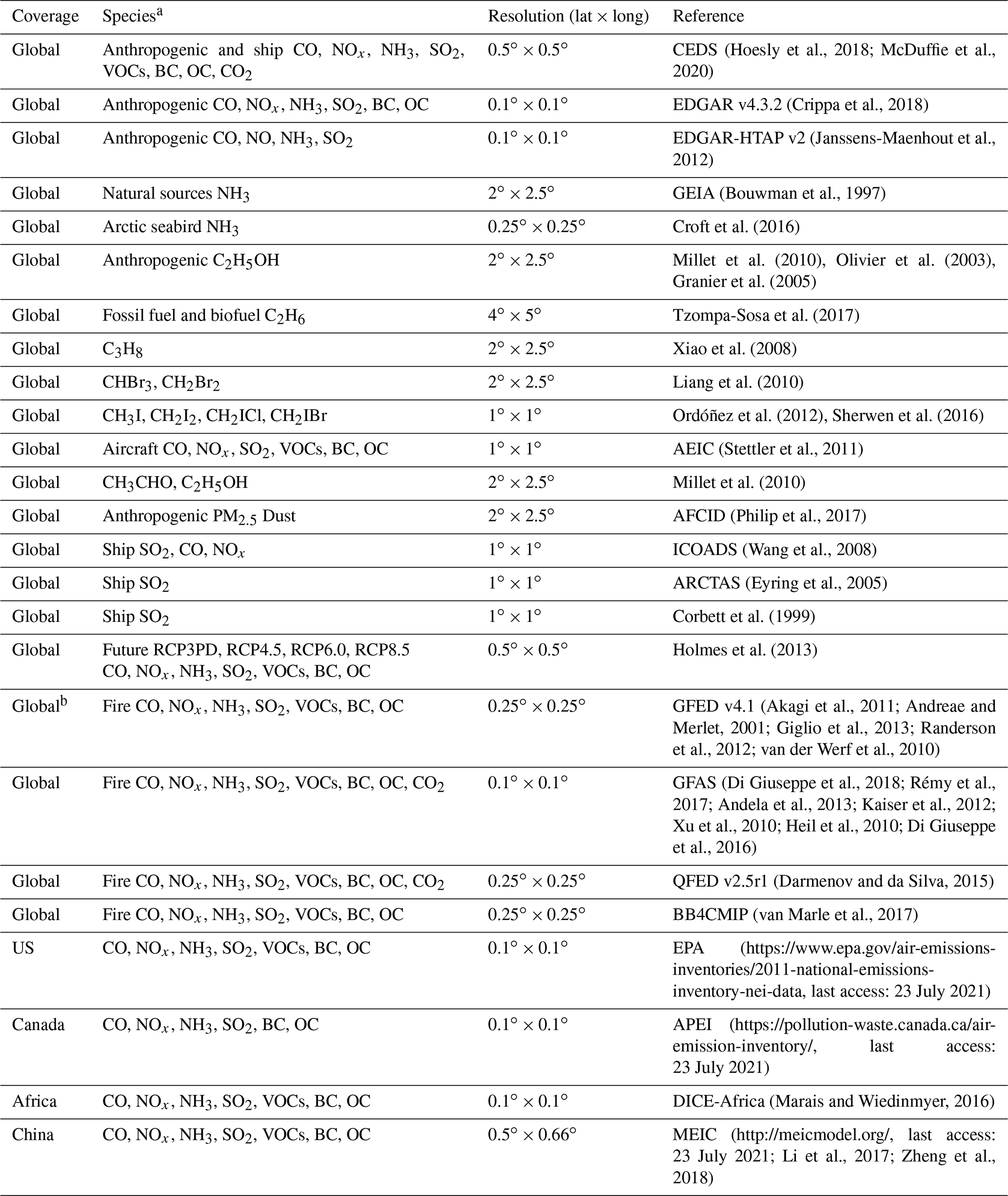
^a VOCs: volatile organic compounds; OC: organic carbon aerosol; BC: black carbon aerosol; ^b implemented as an extension to distribute dry matter input data into model species.

Table 1 lists the emission inventories currently in the HEMCO 3.0 default database library. Users can select from that list and easily add new inventories. The hierarchy of emission inventories is specified in the configuration file. Masking is done by superseding lower-hierarchy inventories with higher-hierarchy inventories so that default inventories may be overwritten by different inventories available only for a particular region, period, or category. For example, an inventory specific for China in 2018 such as MEIC may overwrite a global default inventory. A simulation for later years may retain the Chinese inventory for 2018, scale it up or down, or default to the global inventory, as specified in the configuration file. Additional emission inventories can be added to the HEMCO library in COARDS-compliant NetCDF format. The HEMCO configuration file allows HEMCO to remap variable names in the inventory source file to the species name in the model and specify the region that the inventory is used for and its precedence over the existing entries in the HEMCO library without necessitating preprocessing of the inventory source files.

Emissions dependent on model state such as dust or lightning can be computed online by using algorithms called HEMCO extensions supplied with the HEMCO Core. For example, the current HEMCO Core includes as default the DEAD dust emission extension implementing the algorithm from Zender et al. (2003), but users may select other available extension options (such as the Ginoux et al., 2001, algorithm) or they can add a new algorithm as an extension. Alternatively, users may precompute these emissions based on offline input data and disable the HEMCO extension. Both approaches are routinely used in GEOS-Chem (Weng et al., 2020). Table 2 lists available HEMCO extensions in HEMCO 3.0. Users may add a new algorithm as an extension by creating a new extension file within the “Extensions” directory in HEMCO. HEMCO extensions include subroutines for initialization, run, and finalization. At every time step, the “Run” subroutine receives HEMCO state and model state information and returns the computed emissions array to the HEMCO Core, which can then be added to the other emissions data. New state-dependent emission algorithms can be modified to fit this structure by encapsulating the bulk of the code into the Run routine and adjusting the variable names so that model state can be read through HEMCO. Most HEMCO extensions were developed in this way.

Table 2 Emission extensions available in HEMCO 3.0 as built-in algorithms.

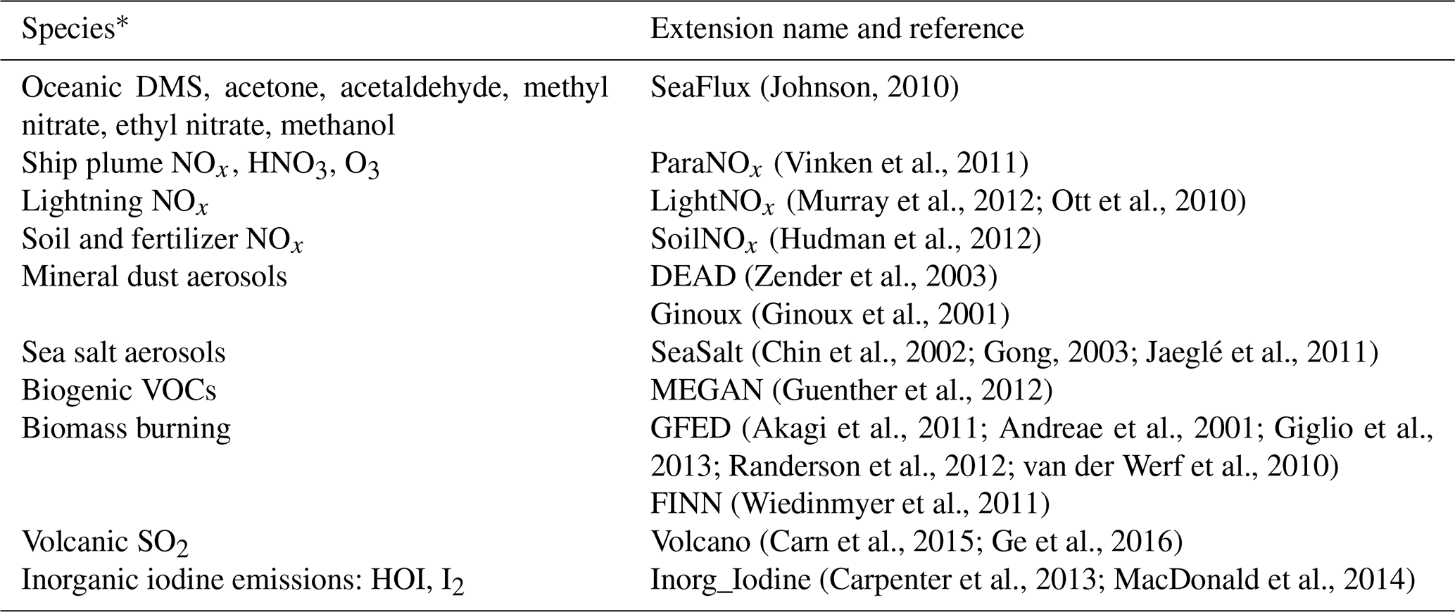
^∗ DMS: dimethyl sulfide.

At the beginning of the run, the Model Interface Layer provides the model species list to the HEMCO Core along with any physical properties needed for computation of state-dependent emissions (for example, Henry's law constants for ocean fluxes). It also provides information to the HEMCO Core on the model environment, such as the model clock and time step size. This information is stored in the HEMCO state by the HEMCO Core.

At every HEMCO time step, when HEMCO is called by the model, the HEMCO Core performs the requested calculations, loading the latest available input data into the HEMCO state's file containers using the Data Input Layer as necessary. Emission fluxes are summed by species, and non-emissions data are stored individually by their data container name (UV albedo example in Fig. 2). The Model Interface Layer then exports the computed fields to the model, interpolating the data to the model grid if it is different than the HEMCO grid. The Model Interface Layer also passes updated model state information to the HEMCO Core for use in extensions (for example, wind speeds to calculate dust emissions). That model state information is re-gridded to the HEMCO grid for the purpose of extension computations.

HEMCO 3.0 computes vertically distributed (3-D) emissions in the same way as 2-D. HEMCO 2.0 assumed the 72-level or 47-level GEOS grid when reading vertically distributed emissions. This required preprocessing of the emission inventory files from their original vertical grids to the supported GEOS grid. Such preprocessing is no longer required in HEMCO 3.0, which reads vertical emission data on any sigma-pressure grid described in the input NetCDF inventory file. The input data are then vertically re-gridded online to the model vertical grid by the Data Input Layer using the MESSy NCREGRID package (Jöckel, 2006). This functionality is used in the WRF-GC and CESM2 models, which have user-configurable vertical grids. HEMCO 3.0 is also capable of distributing 2-D input data on a 3-D grid by modifying the spatial dimension field in the HEMCO configuration file. An example is shown in Fig. 2 where the 2-D NO emission field from the CEDS inventory in the industrial sector is copied vertically to all levels using the flag “xyL*”. Emissions may then be distributed using 3-D scaling factors read from a NetCDF file, such as the scaling factor 316 in Fig. 2. It is additionally possible to emit all 2-D data to a particular level (e.g., to emit to level 5 using “xyL5”) or distributed among an altitude range (e.g., “xyL $=\mathrm{1}:\mathrm{500}$ m” or “xyL $=\mathrm{1}:$ PBL”). Emission heights can additionally be read from a NetCDF file. The spatial dimension parameter can be applied individually to each entry in the HEMCO configuration file and can thus be applied to an individual inventory, sector, or species. Detailed documentation of this capability is available in the HEMCO user guide (http://wiki.seas.harvard.edu/geos-chem/index.php/HEMCO_examples#Applying_2D_emissions_vertically, last access: 8 August 2021).

HEMCO also includes as a diagnostic capability a NetCDF output component to archive selected emissions at specified time steps to disk. This may also include custom diagnostic quantities, such as lightning flash rate from the lightning NO_x extension. The output component is used when HEMCO operates offline in stand-alone mode and also in GEOS-Chem Classic wherein HEMCO handles emission diagnostics. Other target models may have their own diagnostic packages on the model grid, in which case HEMCO diagnostics can be disabled.

2.3 Default Data Input Layer and Model Interface Layer

HEMCO 3.0 includes default out-of-the-box implementations for the Data Input Layer and the Model Interface Layer to enable simple implementation in new models without the need for specific information on model architecture. These default implementations are the ones used in the interface with GEOS-Chem Classic and minimize dependencies on external libraries, facilitating application in a new model environment but with limited features. More advanced implementations are often desirable and will be presented in Sect. 3.

The HEMCO default Data Input Layer is a NetCDF input component with rectilinear latitude–longitude grid re-gridding capabilities. It can be used out of the box in HEMCO with no additional software dependencies. However, it does not support parallel input and as such may be inefficient in a massively parallel model environment. In models that use a non-rectilinear grid for computation or data, it would be necessary to modify the default Data Input Layer if re-gridding is to be performed.

The HEMCO default Model Interface Layer is a module with common utilities for the model to interface with HEMCO. It allows the model to retrieve emission fluxes from HEMCO and control HEMCO subroutines. As the Model Interface Layer is the point of access for the model to interact with HEMCO, implementation of HEMCO in a new model requires a new model interface layer to provide HEMCO with information on the model environment and update model state information for HEMCO extensions.

Implementation of HEMCO in a new model can be prototyped by modifying the default Model Interface Layer to use the model's data structures. The Model Interface Layer includes at least three subroutines: initialization, run, and finalization. These subroutines need to be called by the model and provided with information about the model environment. For initialization, the model species list and their physical properties, the HEMCO grid information, and the location of the configuration file need to be provided. For run, information about the current model time and model state variables for HEMCO extensions needs to be provided, and the computed emissions and data need to be retrieved from the HEMCO Core to be passed back to the model. If the HEMCO grid is different than the model grid (Sect. 2.4), then the Model Interface Layer also needs to implement re-gridding capabilities. An example is HEMCO 3.0's implementation within CESM, as described in Sect. 3.5.

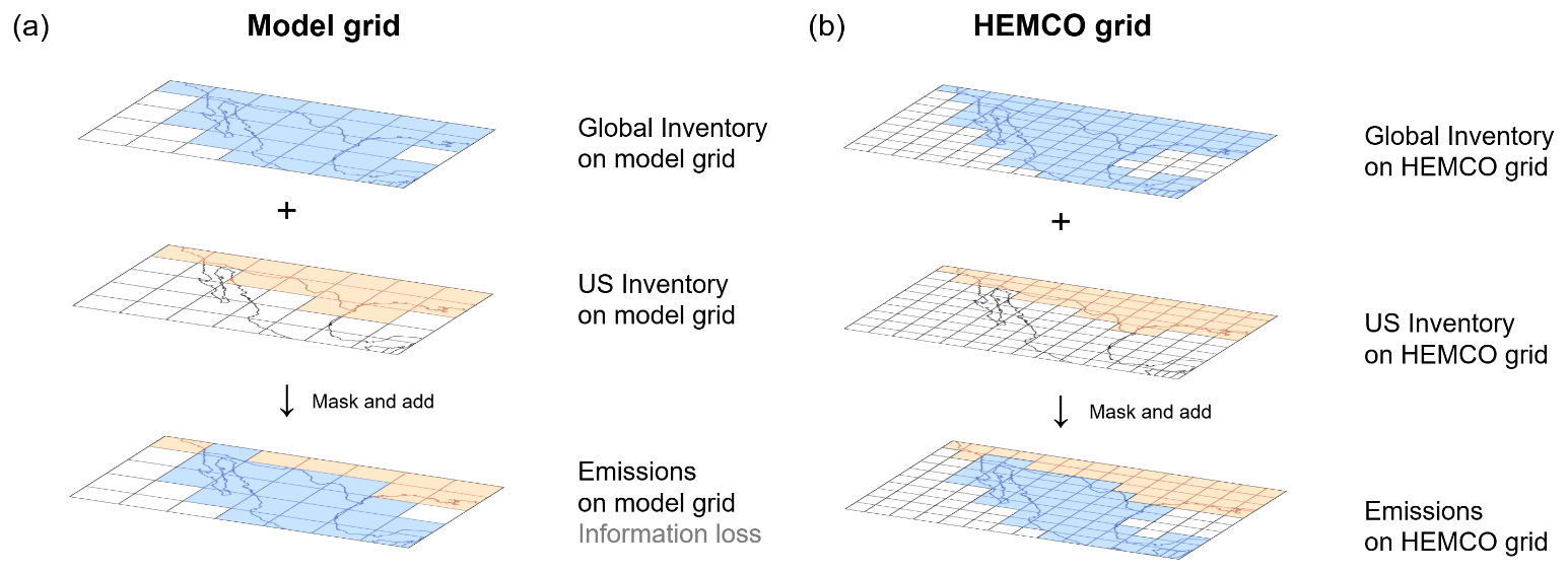
Figure 3 Benefit of using a HEMCO grid finer than the model grid for masking of emissions by a regional inventory. The example in the figure illustrates a case in which a US inventory (orange) is used to replace a global default inventory (blue) in a model simulation on a coarse 4^∘ × 5^∘ grid. The mask is by necessity binary so that US inventory emissions are applied only to grid cells that are 100 % in the US. Using the finer (2^∘ × 2.5^∘) HEMCO grid allows for better resolution of the US–Mexico border and hence for more of the US inventory to be used near the border.

2.4 HEMCO grid

HEMCO 3.0 provides the ability to compute emissions online on a horizontal grid finer than the model grid. Previous versions of HEMCO assumed its operation to be on the same grid as the model. If the model operated multiple grids simultaneously at runtime, as is the case in WRF-GC, multiple instances of HEMCO were used, thus increasing computational and memory cost.

In HEMCO 3.0, a single instance of HEMCO reads and processes data on a user-specified HEMCO grid. When data are requested by the model, the Model Interface Layer re-grids emissions and other data from the HEMCO grid to the model grid. This allows HEMCO to (1) provide data to model components on different grids, (2) operate at a higher resolution for masking and scaling purposes, thus achieving greater accuracy at boundaries between different inventory domains, and (3) use high-resolution environmental datasets when computing emissions through extensions.

Figure 3 illustrates the benefit of using a finer HEMCO grid at the boundaries between inventories. When the HEMCO grid is disabled, HEMCO runs at model resolution, and all input data, including masks, are re-gridded by the Data Input Layer to the model resolution before emissions are computed by the HEMCO Core. In the example of Fig. 3, where a national inventory for the US is to overwrite a global default inventory, this overwriting can be done only for grid cells that are fully in the US. Grid cells straddling the border must retain the global default in order to avoid under- or over-accounting, but this then loses information from the US inventory. This is not a problem if the national inventory straddles the border and includes information on the fractional contributions from the neighboring country, but such is not the case here. Using a finer, intermediate-resolution grid – the HEMCO grid – allows emissions at the model grid scale to more accurately blend the contributions from the two sides of the border in a single model grid cell. This also ensures greater consistency when using the same model simulations at different resolutions. As long as the HEMCO grid is kept at a single resolution, the calculated emissions will be consistent between simulations – no matter what model grid resolution is selected.

Another advantage of using a finer HEMCO grid is for emissions computed with extensions and dependent on both the model variables (provided on the model grid) and environmental data (provided on the HEMCO grid). If there is nonlinear dependence of emissions on the environmental data variables, then a finer HEMCO grid will produce more accurate emissions. This is the case, for example, in dust emission algorithms that use land type as a categorical variable.

There is a limit to the resolution of the HEMCO grid because of the need for HEMCO to store the different inventories in memory, re-grid the data to the HEMCO grid, and process the data at higher resolution, which may be computationally expensive. In global simulations using GEOS-Chem Classic on a single machine at resolutions of 4^∘ × 5^∘ or 2^∘ × 2.5^∘ we have found that a HEMCO grid of 1^∘ × 1.25^∘ is a practical limit. However, masking on the native inventory grid at much higher resolution may be desirable for regional modeling applications. One can circumvent the problem by preprocessing the emissions on their native grids using HEMCO in offline mode. Another option is to use a regional rather than global model. For example, in nested GEOS-Chem Classic simulations at 0.25^∘ × 0.3125^∘ resolution we find that HEMCO can easily handle a HEMCO grid of 0.1^∘ × 0.1^∘, which is typical of the native resolution of inventories.

While any unstructured grid may be used as the HEMCO grid, it may be desirable to use a rectilinear latitude–longitude grid for prototyping HEMCO in new models. This is because the default Data Input Layer provided with HEMCO only supports rectilinear latitude–longitude grids, and most input data available in the HEMCO database library are also on rectilinear latitude–longitude grids. By choosing such a grid, the default Data Input Layer can be readily used for quick prototyping of a new HEMCO implementation, which may then be improved upon if another HEMCO grid is more desirable. In cases in which other grids are used as the HEMCO grid or the model grid, conservative re-gridding needs to be implemented by the Data Input Layer or the Model Interface Layer. Examples of these scenarios are described in Sect. 3.2, where the HEMCO grid is a cubed-sphere grid and ExtData from MAPL with re-gridding capability is implemented as a data input layer, and Sect. 3.5, where the model grid is an arbitrary grid described by an ESMF mesh file provided by the model to HEMCO and ESMF online re-gridding is implemented in the Model Interface Layer.

2.5 Data broker functionality

HEMCO 3.0 has the capability to process any model input data other than emissions such as meteorological fields, land use maps, and boundary conditions. These data can be selected, subsetted (masked), added, and scaled in the same way as emissions. GEOS-Chem has long used this general data broker functionality in HEMCO, but this was previously done by interfacing directly with HEMCO's internal data containers. As this approach bypassed the HEMCO Core, processing of data by the HEMCO Core was also not supported. HEMCO 3.0 standardizes the code for models to retrieve arbitrary data from HEMCO through the Model Interface Layer, thus processing all data from the Data Input Layer through the HEMCO Core. In this manner, HEMCO 3.0 can serve as a general data broker for models if desired.

3 Implementations of HEMCO 3.0 in different models

HEMCO 3.0 has been implemented so far in a number of models: GEOS-Chem Classic, GCHP, NASA GEOS, WRF-GC, CESM2, and NOAA GEFS-Aerosol. It is planned for implementation in the NOAA UFS. These models have different architectures and software engineering environments, requiring different formulations of the Data Input Layer and Model Interface Layer with the same HEMCO Core. We describe below the particularities of implementation for each model as a guide for implementation in other models.

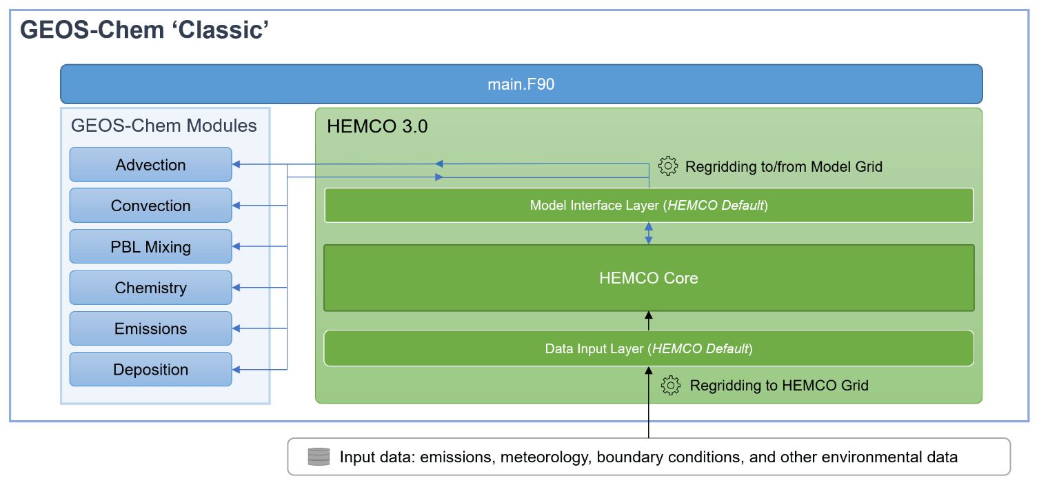
Figure 4 HEMCO 3.0 implementation in the GEOS-Chem Classic model. HEMCO in GEOS-Chem Classic is a general input data broker. The main model driver routine main.F90 successively calls each GEOS-Chem module and HEMCO in a time step loop. HEMCO 3.0 reads all input data through the default Data Input Layer, processes the data through the HEMCO Core, and exports the data to each GEOS-Chem module through the HEMCO default Model Interface Layer. The Model Interface Layer also receives data from GEOS-Chem modules that are used by HEMCO to compute state-dependent emissions through extensions.

3.1 GEOS-Chem “Classic”

GEOS-Chem Classic (Bey et al., 2001) is an offline chemical transport model (CTM) driven by NASA GEOS meteorological data. It operates on global or regional (nested) rectilinear latitude–longitude grids. It uses OpenMP shared-memory parallelization on a single node without a dedicated coupler. Figure 4 shows the implementation of HEMCO 3.0 in GEOS-Chem Classic as both an emissions component and a general input data broker. The default Data Input Layer is used to read and re-grid all input data, which are then processed through the HEMCO Core. When the HEMCO grid is different than the model grid (Sect. 2.4), the Model Interface Layer performs horizontal re-gridding between the two grids for the data flowing through it.

HEMCO 3.0 in GEOS-Chem Classic is used for all gridded input data including not only emissions but also meteorological fields, chemical boundary conditions (for regional runs), initial conditions, and other environmental datasets such as land type, leaf area index, and sea surface salinity. It serves as a re-gridding and subsetting tool for these data. This has in particular enabled the FlexGrid capability in GEOS-Chem wherein regional nested domains are selected at runtime and all input data are processed for these domains (Li et al., 2021; Shen et al., 2021).

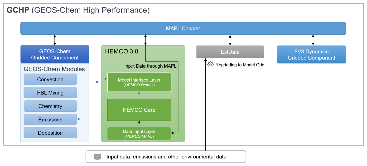
Figure 5 HEMCO 3.0 implementation in the GEOS-Chem High-Performance model (GCHP). GCHP operates under the MAPL coupling framework in an MPI parallel environment. The ExtData component reads all data into MAPL, re-gridding them to the model grid, and the input data are retrieved by the HEMCO MAPL implementation of the Data Input Layer. After emissions are processed by the HEMCO Core, they are exported to GEOS-Chem through the HEMCO default Model Interface Layer.

Figure 6 HEMCO 3.0 implementation in the NASA GEOS Earth System Model. GEOS is driven by the MAPL framework in an MPI parallel environment and is composed of a number of gridded components for the different ESM operators. GOCART provides a fast aerosol simulation and GEOS-Chem provides detailed chemistry. HEMCO serves both GOCART and GEOS-Chem. The ExtData component reads all data into MAPL, re-gridding them to the model grid, and the input data are retrieved by the HEMCO MAPL implementation of the Data Input Layer. GEOS-Chem and GOCART each have their own HEMCO instances. After emissions are processed by the HEMCO Core, they are exported to GEOS-Chem through the HEMCO default Model Interface Layer and to the GOCART gridded component through a HEMCO gridded component model interface layer.

3.2 GEOS-Chem High Performance (GCHP)

GCHP (Eastham et al., 2018; Zhuang et al., 2020) is a high-performance version of GEOS-Chem that takes advantage of the grid-independent structure of the model (Long et al., 2015) to apply a distributed-memory MPI parallelization enabling efficient simulations with thousands of cores. Implementation of MPI is through the GEOS MAPL environment on cubed-sphere grids. MAPL is a modeling toolkit built upon ESMF that provides additional tools for interfacing between ESMF and the model code (Suarez et al., 2007). It serves as a coupler for individual model components, referred to as “gridded components”, and provides input and cubed-sphere re-gridding capabilities for all external data through the ExtData component. GCHP advection is computed by the FV3 dynamical core gridded component (Putman and Lin, 2007).

Figure 5 shows the implementation of HEMCO 3.0 in GCHP. In the MAPL environment, all data are read and re-gridded to the model grid by the ExtData component. Thus, HEMCO in MAPL uses the MAPL data input layer, which simply retrieves data from ExtData. Unlike in GEOS-Chem Classic, meteorological data are not processed by HEMCO in GCHP, as these data are provided to GEOS-Chem through ExtData. There is also no option for HEMCO to operate on a HEMCO grid different from the model grid because ExtData re-grids all data to the model grid.

After emissions data are processed by the HEMCO Core, GEOS-Chem receives the emissions from HEMCO through the HEMCO default Model Interface Layer in the same manner as GEOS-Chem Classic. In this manner, the interface between the GEOS-Chem emissions module and HEMCO is the same for GEOS-Chem Classic and GCHP, facilitating the maintenance of a single GEOS-Chem code.

3.3 NASA GEOS ESM

The GEOS ESM (Rienecker et al., 2008) provides the platform for Earth system data analysis at NASA through the GEOS Data Assimilation System (GEOS-DAS). It has several options for online representation of atmospheric chemistry including GEOS-Chem (Hu et al., 2018) and GOCART aerosols (Chin et al., 2002; Randles et al., 2017). GOCART is used in the operational GEOS-DAS as a fast module for aerosol data assimilation. The GEOS-Chem module is used in the GEOS chemical forecast product (GEOS-CF; Keller et al., 2020) and in research applications. It has exactly the same code as the offline GEOS-Chem but with all transport routines disabled, since chemical transport is done as part of the GEOS ESM atmospheric dynamics.

Figure 6 shows the implementation of HEMCO 3.0 in the GEOS ESM to serve both the GEOS-Chem and GOCART modules. HEMCO 3.0 receives data from the MAPL data input layer using ExtData to read in data and re-gridding to the cubed-sphere grid in the GEOS ESM. The data passed to HEMCO through ExtData are limited to emissions, as all other data are generated through the GEOS model or introduced elsewhere.

The GEOS ESM uses separate instances of HEMCO for interfacing with GEOS-Chem and GOCART. These separate instances use different HEMCO configuration files and run independently of each other in parallel. For interfacing with GEOS-Chem, HEMCO uses the default Model Interface Layer in the same manner as GCHP (Sect. 3.2). This enables usage of GEOS-Chem chemistry within GEOS with minimal changes to the GEOS-Chem code. For interfacing with GOCART, HEMCO exports data using MAPL through a separate HEMCO gridded component model interface layer, and those data are then imported by GOCART.

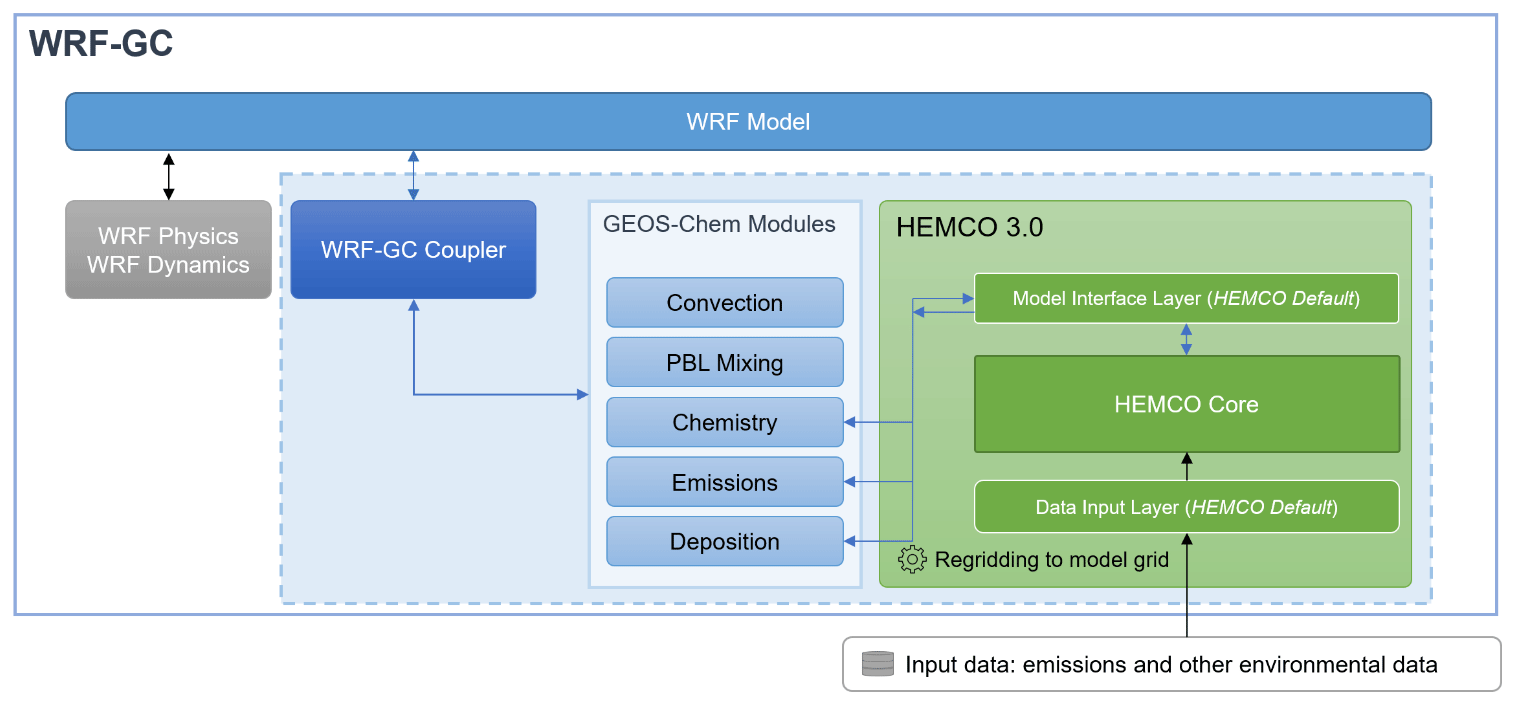
Figure 7 HEMCO 3.0 implementation in the WRF-GC model. The model is driven by WRF, which calls GEOS-Chem chemistry through the WRF-GC coupler. HEMCO 3.0 is implemented entirely as part of GEOS-Chem in WRF-GC, with each successive domain in the WRF model containing a separate instance of GEOS-Chem and HEMCO (dashed blue box). HEMCO interfaces with GEOS-Chem using the HEMCO default Model Interface Layer and reads data through the HEMCO default Data Input Layer using the same approach as GEOS-Chem Classic. Convection and PBL mixing are done by GEOS-Chem modules, but the driving meteorological data are provided by the WRF-GC coupler instead of through HEMCO, unlike in GEOS-Chem Classic.

3.4 WRF-GC

The WRF-GC online model (Weather Research and Forecasting Model with GEOS-Chem chemistry; Lin et al., 2020; Feng et al., 2021) couples the Weather Research and Forecasting (WRF) weather model (Skamarock et al., 2008) with GEOS-Chem in the same manner as the coupling of WRF with WRF-Chem (Grell et al., 2005; Fast et al., 2006). It uses a WRF-GC coupler separate from the WRF and GEOS-Chem parent models to interface between the two models, converting the state between WRF and GEOS-Chem as necessary to drive both models. This coupling structure enables independent updates of each model in WRF-GC. Chemical advection is done by WRF, but convection and planetary boundary layer (PBL) mixing are done by GEOS-Chem using input data from WRF, following the practice in WRF-Chem. Aerosol effects on WRF radiation and cloud physics are treated by passing GEOS-Chem aerosol information to WRF through the WRF-GC coupler. Multiscale WRF grids communicating by two-way nesting are also supported by WRF-GC.

Figure 7 shows the implementation structure of HEMCO within the WRF-GC model. In WRF-GC, HEMCO is implemented as a component within GEOS-Chem using the same default Data Input Layer and default Model Interface Layer as GEOS-Chem Classic. The Data Input Layer reads emissions and environmental data to serve GEOS-Chem emissions, chemistry, and dry deposition routines. Meteorological data simulated by WRF (including convective air mass fluxes, PBL mixing parameters, and any meteorological data needed for HEMCO extensions) are passed to GEOS-Chem by the WRF-GC coupler independently of HEMCO. Chemical initial and boundary conditions are also read by the WRF model and passed to GEOS-Chem through the WRF-GC coupler. If there are successive instances of WRF for nested domain functionality, corresponding instances of GEOS-Chem and HEMCO for each domain are used. Each instance of HEMCO operates on the grid of the corresponding WRF domain, and no separate HEMCO grid is used.

Figure 8 HEMCO 3.0 implementation in CESM2. HEMCO 3.0 lives as a component within the CESM2 atmosphere (CAM), reading data through the HEMCO default Data Input Layer and communicating with other CESM components through the HEMCO–CESM implementation of the Model Interface Layer, which reads necessary meteorological quantities for computation of state-dependent emissions within HEMCO and exports emissions and other input data to the CAM physics buffer. HEMCO operates on its own high-resolution grid, with re-gridding routines to pass data to and from CAM. Environmental data for computing emissions and dry deposition (e.g., land type) may either be read from HEMCO data libraries or provided to HEMCO by the CAM state.

3.5 Community Earth System Model Version 2 (CESM2)

The Community Earth System Model Version 2 (CESM2) is an open-source model enabling a wide range of Earth science simulations including atmospheric chemistry. The atmospheric component of CESM2 is the Community Atmosphere Model (CAM), including the CAM-chem module to simulate chemistry (Emmons et al., 2020). The new MUSICA initiative at NCAR (Pfister et al., 2020) seeks to expand the capabilities and versatility of the chemical simulation within CAM, including use of GEOS-Chem as an alternative module.

Figure 8 shows the implementation of HEMCO 3.0 in CESM2. HEMCO serves emissions to CAM-chem, GEOS-Chem, and potentially to any representation of atmospheric chemistry in CAM. The Model Interface Layer includes routines to export data processed by HEMCO to CAM's physics buffer, a temporary storage space for model components to share data at runtime. As CAM supports a variety of grids, during initialization, the HEMCO–CESM Model Interface Layer reads the ESMF mesh file that describes the grid used by CAM and uses ESMF online re-gridding (https://earthsystemmodeling.org/regrid/, last access: 2 September 2021) to re-grid data between HEMCO and CAM. By using ESMF re-gridding capabilities, HEMCO is capable of operating independently of the grid used by the model, as long as the model grid description is provided to HEMCO using an ESMF mesh file.

HEMCO within CESM2 can use the existing HEMCO emissions database library out of the box, and it can also import new emission inventories and extensions. The CAM-chem implementation uses a configuration file with the appropriate CAM-chem species mapping as described by Emmons et al. (2020). An example for alcohols was described in Sect. 2.1. For CESM with GEOS-Chem chemistry (CESM2-GC), HEMCO works out of the box with configuration files from GEOS-Chem since CESM2-GC uses the same species.

Environmental data needed for computing emissions and dry deposition, such as land type and leaf area index, are normally provided by the CESM state to HEMCO through the Model Interface Layer. This is required for coupled chemistry–biosphere–climate simulations, wherein atmospheric chemistry affects ecosystem state (both directly and indirectly through the climate), which in turns affects atmospheric chemistry. Alternatively, one may want to use independent environmental data specified through the HEMCO configuration file in order to compare the CESM simulation to an independent simulation of atmospheric chemistry such as with GEOS-Chem Classic. Both capabilities are supported by HEMCO within CESM2.

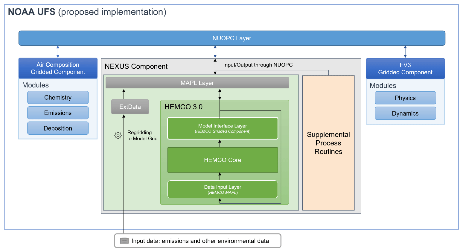
Figure 9 Planned HEMCO 3.0 implementation in the NOAA UFS. UFS is a unified software infrastructure for NOAA forecast models to enable exchange of model components between different application models. HEMCO is planned as the core of the NOAA Emissions and eXchange Unified System (NEXUS) component to serve both emissions and surface exchange (state-dependent emissions, dry deposition, and two-way exchange) as part of UFS. HEMCO operates under the MAPL coupling framework in the same way as in the NASA GEOS ESM (Fig. 6) but reads independent environmental data for use in surface exchange calculations. Supplemental process routines provide the surface exchange calculations. NEXUS operates under the NUOPC coupling framework to provide emissions and surface exchange information to other UFS components.

3.6 NOAA GEFS-Aerosol and NOAA UFS

As described in NOAA's 2018 Strategic Implementation Plan for next-generation modeling systems (https://www.weather.gov/sti/stimodeling_nggps_implementation, last access: 2 September 2021), “a unified emission system with the capability of providing model-ready, global anthropogenic and natural source emissions inputs for aerosol and gas-phase atmospheric composition across scales is needed.” The next-generation modeling systems of NOAA are being realized as the Unified Forecast System (UFS; https://ufscommunity.org, last access: 2 September 2021), which will replace the current suite of forecast models in the National Weather Service (NWS) over the next few years. The UFS does not refer to a single modeling system, but rather describes a unified software infrastructure that permits the exchange of model components between different application models. To respond to the requirement for a unified emissions system, HEMCO 3.0 is being tested to serve as the core of the NOAA Emissions and eXchange Unified System (NEXUS) component (Campbell et al., 2020). NEXUS will provide emissions and broader surface exchange information for NOAA's UFS global and regional aerosol and atmospheric composition (AAC) models.

Figure 9 shows the planned implementation of HEMCO as the core of NEXUS within the NOAA UFS. Currently, HEMCO is used as an offline emissions preprocessor for an experimental version of the Global Ensemble Forecast System-Aerosol (GEFS-Aerosol). GEFS-Aerosol is a global aerosol model based on the Global Forecast System (GFS), which is based on the finite-volume cubed-sphere (FV3) dynamical core (Lin et al., 1994; Lin and Rood, 1996; Lin, 2004; Putman and Lin, 2007; Chen et al., 2013; Harris and Lin, 2013; Harris et al., 2016; Zhou et al., 2019). The operational version of GEFS-Aerosol is run by the NWS as a special unperturbed forecast of the Global Ensemble Forecast System version 12, which provides an ensemble forecast product four times per day.

Ongoing development of NEXUS includes adaptation to provide emissions for three future UFS applications: (i) a global aerosol model, adapted from GEFS-Aerosol, that will be part of a sub-seasonal to seasonal forecast capability and that uses the NASA GOCART aerosol model; (ii) an online, regional-scale air quality model with fully coupled gas-aerosol chemistry derived from the Community Multiscale Air Quality (CMAQ) model (United States Environmental Protection Agency, 2018); and (iii) an online, regional-scale rapid refresh forecast system (RRFS) that includes fully coupled smoke and dust emissions as well as transport and aerosol–weather interactions. Further planned development of NEXUS for UFS AAC models includes the integration of HEMCO 3.0 as a dynamic online emissions processor for both anthropogenic inventories and natural, process-based sources (e.g., windblown dust, wildfire smoke, sea salt). A longer-term goal for NEXUS includes the harmonization of emissions-related processes with the surface–atmosphere exchange and boundary layer processes in the land surface modeling system. The current vision for the NEXUS architecture is evolving as the UFS AAC models are being developed but will rely on established coupling and integration infrastructures, such as the National Unified Operational Prediction Capability (NUOPC) layer (Theurich et al., 2016; http://earthsystemmodeling.org/nuopc/, last access: 2 September 2021).

4 Conclusions

We presented an updated version 3.0 of the Harmonized Emissions Component (HEMCO 3.0) for atmospheric models. HEMCO is a versatile online emissions processor originally developed for the GEOS-Chem chemical transport model but is now portable to any atmospheric model. HEMCO allows users to select an ensemble of emission inventories and state-dependent emission algorithms (extensions) with capabilities for re-gridding, adding, masking, and scaling emission data and mapping them to model species. HEMCO 3.0 addresses limitations of the previous version, HEMCO 2.0, which used features specific to the GEOS-Chem “Classic” or MAPL environments and was limited to operating on the model grid. HEMCO 3.0 has a modular structure to facilitate its implementation in models with different software engineering protocols. It features an optional high-resolution grid that may be finer than the model grid for more accurate masking, more accurate computation of emissions with nonlinear algorithms, and the serving of emission data to multi-grid models with greater computational and memory efficiency. HEMCO 3.0 can also serve as a general data broker to process all input data in the atmospheric model, not just emissions.

HEMCO 3.0 modularizes the original HEMCO (Keller et al., 2014) into three layers: the Data Input Layer, the HEMCO Core, and the Model Interface Layer. The Data Input Layer reads a configuration file that defines the emission environment desired by the user, extracts the necessary inventory and other data files in NetCDF format from the HEMCO database library, and re-grids the data to the model grid or to the higher-resolution HEMCO grid. The HEMCO Core subsets, adds, masks, and scales the different datasets as specified by the configuration file. The Model Interface Layer collects the emissions data from the HEMCO Core to pass on to the atmospheric model and also passes model state variables to the HEMCO Core for computing emissions through extensions. The HEMCO Core and database library are common to HEMCO implementations across all models. The Data Input Layer and Model Interface Layer may be used out of the box or modified to fit a model's specific architecture.

HEMCO 3.0 has been implemented in several models: the GEOS-Chem CTM in both Classic and High-Performance (GCHP) configurations, the NASA GEOS ESM, WRF with GEOS-Chem chemistry (WRF-GC), CESM2 with either CAM-chem or GEOS-Chem chemistry, and the NOAA GEFS-Aerosol model as an offline emissions preprocessor. GEOS-Chem Classic relies on the default implementations of the Data Input Layer and Model Interface Layer, and these defaults may be used for quick implementation of HEMCO 3.0 in any model. GCHP and the GEOS ESM use the MAPL coupler built on ESMF to read and re-grid data; in that case the corresponding functionalities are removed from the HEMCO Data Input Layer with no editing of code in the HEMCO Core. HEMCO 3.0 is planned for inclusion in the NOAA UFS as the core of the NEXUS component that will serve emission and surface exchange information to the suite of NOAA aerosol and atmospheric composition forecast models. This will add a new dimension to HEMCO capabilities to include surface deposition and two-way exchange of chemical species.

Implementation of HEMCO 3.0 in CESM2 is an important step in the development of MUSICA, a flexible modeling framework for the next-generation CESM allowing for versatile use of different atmospheric chemistry simulation components on any grid and scale (Pfister et al., 2020). HEMCO within CESM can operate on multiscale or unstructured grids, can serve data to any CESM atmospheric component, and can interface with any chemical mechanism by mapping emitted species to the mechanism species. Through HEMCO, CESM users can readily use and combine any ensemble of emission inventory data and algorithms that they choose independently of their chemical mechanism or other aspects of the chemical simulation. HEMCO thus provides a general vessel for the treatment of emissions in MUSICA and could also provide a general input data broker facility for CESM in the future.