the Creative Commons Attribution 4.0 License.
the Creative Commons Attribution 4.0 License.
 | 23 Aug 2021
PALEOSTRIPv1.0 – a user-friendly 3D backtracking software to reconstruct paleo-bathymetries
Florence Colleoni
Laura De Santis
Enrico Pochini
Edy Forlin
Riccardo Geletti
Giuseppe Brancatelli
Magdala Tesauro
Martina Busetti
Carla Braitenberg
Paleo-bathymetric reconstructions provide boundary conditions to numerical models of ice sheet evolution and ocean circulation that are critical to understanding their evolution through time. The geological community lacks a complex open-source tool that allows for community implementations and strengthens research synergies. To fill this gap, we present PALEOSTRIPv1.0, a MATLAB open-source software designed to perform 1D, 2D, and 3D backtracking of paleo-bathymetries. PALEOSTRIP comes with a graphical user interface (GUI) to facilitate computation of sensitivity tests and to allow the users to switch all the different processes on and off and thus separate the various aspects of backtracking. As such, all physical parameters can be modified from the GUI. It includes 3D flexural isostasy, 1D thermal subsidence, and possibilities to correct for prescribed sea level and dynamical topography changes. In the following, we detail the physics embedded within PALEOSTRIP, and we show its application using a drilling site (1D), a transect (2D), and a map (3D), taking the Ross Sea (Antarctica) as a case study. PALEOSTRIP has been designed to be modular and to allow users to insert their own implementations.
- Article
(9957 KB) - Full-text XML
- BibTeX
- EndNote


Ongoing climate changes are urging the scientific community to project future climate evolution in response to carbon emission trajectories (e.g. the Shared Socio-economical Pathways by Riahi et al., 2017). The Coupled Model Intercomparison Project (CMIP), now ending phase 6 (Eyring et al., 2016), has been producing a large amount of climate projections that extend to 2100. However, some of the climatic variables, e.g. the deep ocean, the carbon cycle, and the ice sheets and glaciers, react more slowly to climate changes (e.g. Colleoni et al., 2018b; Noble et al., 2020), despite already showing evidence of changes over the past few decades (Caesar et al., 2021). Their main response has yet to be observed and is likely to happen beyond the 21st century, which is encouraging climatologists to project changes on longer timescales that cover centuries to millennia into the future (e.g. IPCC, 2013, 2019). Projecting to such timescales implies designing corresponding realistic carbon emission trajectories, and so far millennial-scale emissions trajectories are just extension of existing emission scenarios beyond 2100 (e.g. Golledge et al., 2015; DeConto and Pollard, 2016). At this point, the exercise becomes difficult, and this is when reconstructing past climates becomes important. It allows for the testing of the response of the Earth's climate under different but realistic atmospheric greenhouse gas (GHG) concentrations (e.g. Haywood et al., 2019). GHG concentrations higher than present-day or future levels, i.e. larger than 400 ppm for atmospheric CO2, can only be found for times prior to 3 million years ago (e.g. Zhang et al., 2013; Bracegirdle et al., 2019). Going back to those times (or even before), it is likely that the tectonic setting responsible for other boundary conditions, such as oceanic gateways, elevation of mountain ranges, continental margin expansion, and the location and extent of continental masses themselves, differed from that of the present-day (e.g. Herold et al., 2008; Frigola et al., 2018; Müller et al., 2018a; Straume et al., 2020; Hochmuth et al., 2020). Nevertheless, simulating and reconstructing past climatic conditions can bring useful hints as to how the future climate might evolve and also help in narrowing the range of likely long-term carbon emissions trajectories.
Reconstructing past topographies and bathymetries is fundamental for paleoclimate and paleo-ice-sheet simulations (e.g. Otto-Bliesner et al., 2017; Colleoni et al., 2018a; Straume et al., 2020; Paxman et al., 2020). The numerous oceanic deep-drilling campaigns that occurred over the past decades have the potential to constrain such reconstructions, but this is not the case when part of the information has been eroded and/or reworked during geological time by other tectonic or climatic processes. In addition, during sediment deposition, the bathymetry itself changes due to different processes, such as the loading of accumulated sediments, thermal subsidence acting on extended continental crust, or subsidence or uplift induced by mantle dynamics (dynamic topography) or sea level changes (e.g. Kirschner et al., 2010; Celerier, 1988; Sclater and Christie, 1980). Other external factors also influence the bathymetry, e.g. ice loading in polar areas. When accounting for all those factors and processes by decompacting and removing overlying sediments, it is possible to backtrack the bathymetry, and thus the paleo-water depth, of a chosen specific time interval. Conversely, if the target of the study is to reconstruct the burial history of a sedimentary basin, the technique is the same but needs constraints on the paleo-water depths and is called “backstripping” (Steckler and Watts, 1978).
There are few existing open-source backstripping or backtracking codes. Flex-Decomp by Badley Geoscience Ltd. (Kusznir et al., 1995) allows for 2D-flexural backstripping or backtracking, but its code is not open-source. A 3D version of Flex-Decomp exists, but it is not open-source (Roberts et al., 2003) and is used exclusively by Badley Geoscience Ltd. and is thus not available externally. It comes along with the sister programme Stretch by Badley Geoscience Ltd., a software used to compute forward modelling of basin evolution that provides a spatially variable stretching factor cross section to be used by Flex-Decomp. BasinVis (Lee et al., 2016, 2020) is a MATLAB open-source code with a graphical user interface. It calculates compaction trends from input drill site (1D) lithological units. The estimated compaction trends can be applied in thickness restoration of stratigraphic units and subsidence analysis data that can be spatially interpolated between input drill sites to reconstruct a temporal basin evolution. Dressel et al. (2015, 2017) perform 3D backtracking of the southwestern African continental margin while accounting for 1D thermal subsidence and Pratt isostasy, taking into account lateral density variations. PyBacktrack is a 1D backtracking and backstripping open-source code (Müller et al., 2018b) aimed at reconstructing paleo-bathymetries. It allows the processing of drilling sites both on oceanic and continental crust; can be connected to the suite of geodynamical open-source software GPlates (https://www.gplates.org/, last access: August 2021); and benefits from geodynamical corrections related to kinematic, tectonic, and geodynamic models of tectonic plate movements through time. DeCompactionTool (Hölzel et al., 2008) proposes a similar approach to pybacktrack (also in 1D) but allows for the performing of a Monte Carlo style analysis, i.e. performing a large number of 1D runs based on a possible range of main physical parameters defined by admissible minimum and maximum values to provide a quantitative estimate of the backstripping error.
Both 3D flexural backstripping and backtracking are needed to reconstruct basin-wide or continental-wide areas that will be prescribed as boundary conditions within climate and ice sheet models. A few studies mentioned the use of 3D backstripping (e.g. Scheck et al., 2003; Hansen et al., 2007; Smallwood, 2009; Amadori et al., 2017), and a very limited number of studies provide this with 3D flexural backstripping (Roberts et al., 2003; Steinberg et al., 2018; Roberts et al., 2019).
Here we present PALEOSTRIP, a MATLAB open-source software designed to perform 1D, 2D, and 3D backtracking of paleo-bathymetries. PALEOSTRIP comes with a graphical user interface (GUI) to facilitate computation of sensitivity tests and allows the users to switch all of the different processes on and off and thus separate the various aspects of backtracking. As such, all physical parameters can be modified from the GUI. It includes 3D flexural isostasy, 1D thermal subsidence, and possibilities to correct for prescribed sea level and dynamical topography changes. In the following, we detail the physics embedded within PALEOSTRIP and show a few applications for a drilling site (1D), a transect (2D), and a map (3D), taking the Ross Sea (Antarctica) as a case study.
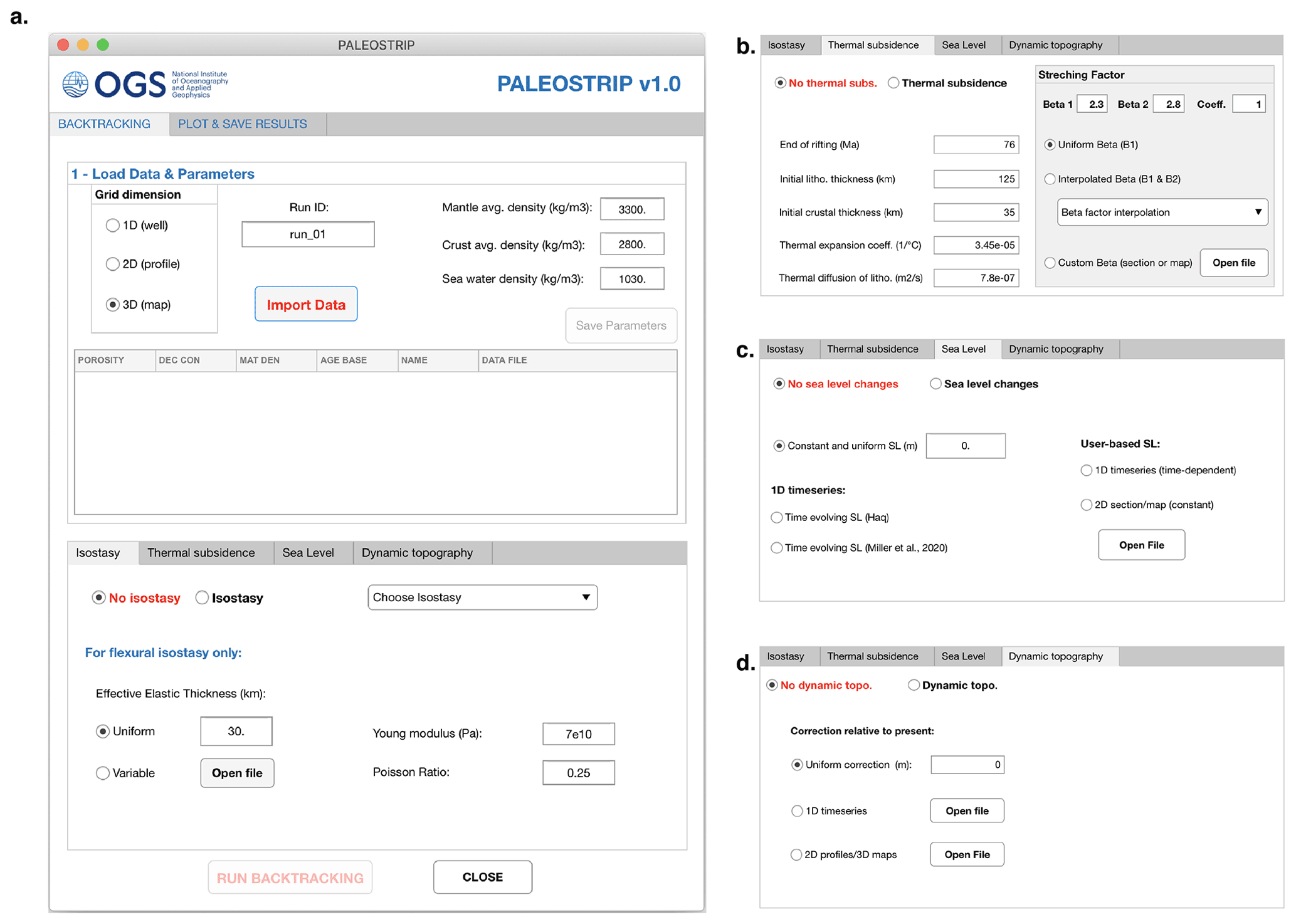
Figure 1Example of the PALEOSTRIP application GUI, showing this following elements: (a) the main PALEOSTRIP GUI, (b) tab interface to set thermal subsidence (bottom of main GUI), (c) tab interface to set sea level corrections, and (d) tab interface to set dynamic topography correction.
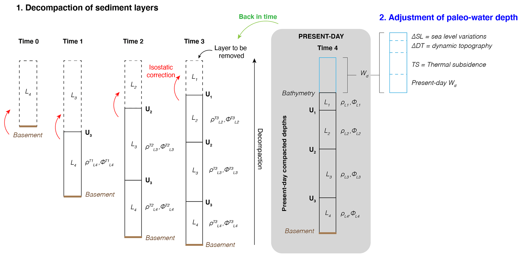
Figure 2The backtracking procedure used in PALEOSTRIP is as follows. Sediment layers L are separated by well-defined seismic or lithological unconformities U. All the sediment layers have different lithological properties defined by their porosity ϕ and density ρ. These two properties change during the decompaction process, departing from the present-day depth of sediment layers, as buried sediments are unloaded from the upper sediment layers (isostatic correction). The water depth at each time step is calculated using a time-varying thermal subsidence model (Eq. 3).
PALEOSTRIP is a MATLAB open-source code developed under the GNU General Public License v3.0. It is composed of a set of routines accessed using a graphical interface from which users can load data, change physical parameters, and plot and save results (Fig. 1). The code is distributed on GitHub (https://github.com/flocolleoni/PALEOSTRIPv1.0, last access: August 2021) alongside a user manual providing all necessary explanations and examples of how to input data and use PALEOSTRIP functionalities. Note that the final version related to this study has been corrected for minor bugs and that the main “plot and save” graphical interface has been modified to implement 12 colour scales, including 9 colour-blind-friendly scales from Crameri et al. (2020). We thus again invite the readers to download the code from GitHub and from Zenodo.
PALEOSTRIP has been designed and coded with MATLAB (2019) and runs on any operating system. Most of the code should be compatible with previous versions of MATLAB, provided that it includes the App Designer toolbox (https://it.mathworks.com/products/matlab/app-designer.html, last access: August 2021). The code is incompatible with GUIDE and from MATLAB R2020 onwards GUIDE is no longer available. PALEOSTRIP cannot be run without its graphical interface, and thus a version of MATLAB with the App Designer toolbox is necessary.
2.1 PALEOSTRIP graphical user interface
PALEOSTRIP graphical user interface (GUI) is composed of two different tabs. The first one is dedicated to input data, physical parameters, and choices of physical methods for each of the processes accounted for in backtracking (Fig. 1). The second one is dedicated to plotting backtracked data and saving results (see Sect. 6). The GUI can be launched either through the MATLAB main interface and double-clicking on the corresponding App Designer GUI file or by exporting it as a stand-alone application that can be executed without opening MATLAB. We do not provide a built-in PALEOSTRIP application, since the compilation of the applications depends on the operating system on which it is created, but we provide the PALEOSTRIP code instead. As such, the user is free to export it from the App Designer tool.
2.2 Format of input and output data
2.2.1 Coordinate system
Cartesian coordinates (in m) are required to perform flexural isostasy calculations, as the flexural response depends on the distance from the load. Consequently, input data must be provided on a Cartesian coordinate grid. PALEOSTRIP does not run on geographical coordinates and does not provide any tool to convert input data from geographical to Cartesian coordinates. However, many examples of open-source software or code exist to perform this step, such as the MATLAB Mapping Toolbox (https://it.mathworks.com/products/mapping.html, last access: August 2021), Generic Mapping Tools 6 (https://www.generic-mapping-tools.org/, last access: August 2021), OBLIMAP2 (Reerink et al., 2016), or any other geographic information system (GIS) software.
2.2.2 Input files
Horizon depths have to be provided individually in single ASCII files, defining the given quantity along with its coordinates. For example, horizon depth Z for a 1D drill site, extension along the transect and depth (X,Z) for 2D transects, and the horizontal position (X,Y) and depth (Z) for 3D horizon maps. Output data are saved with the same format. PALEOSTRIP does not read and write grids in the NetCDF format. Lithological parameters must be provided in a separate ASCII file and are spatially uniform. In the present study, the input data files associated with each case study are zipped in paleostrip_examples.zip, available on GitHub at (https://github.com/flocolleoni/PALEOSTRIPv1.0, last access: August 2021). Since the lithological parameters vary substantially given the composition of sediments and their depositional context, we refer the reader to Kominz et al. (2011) for values and detailed explanations on how to retrieve the decompaction coefficients for the different lithologies of marine sediments.
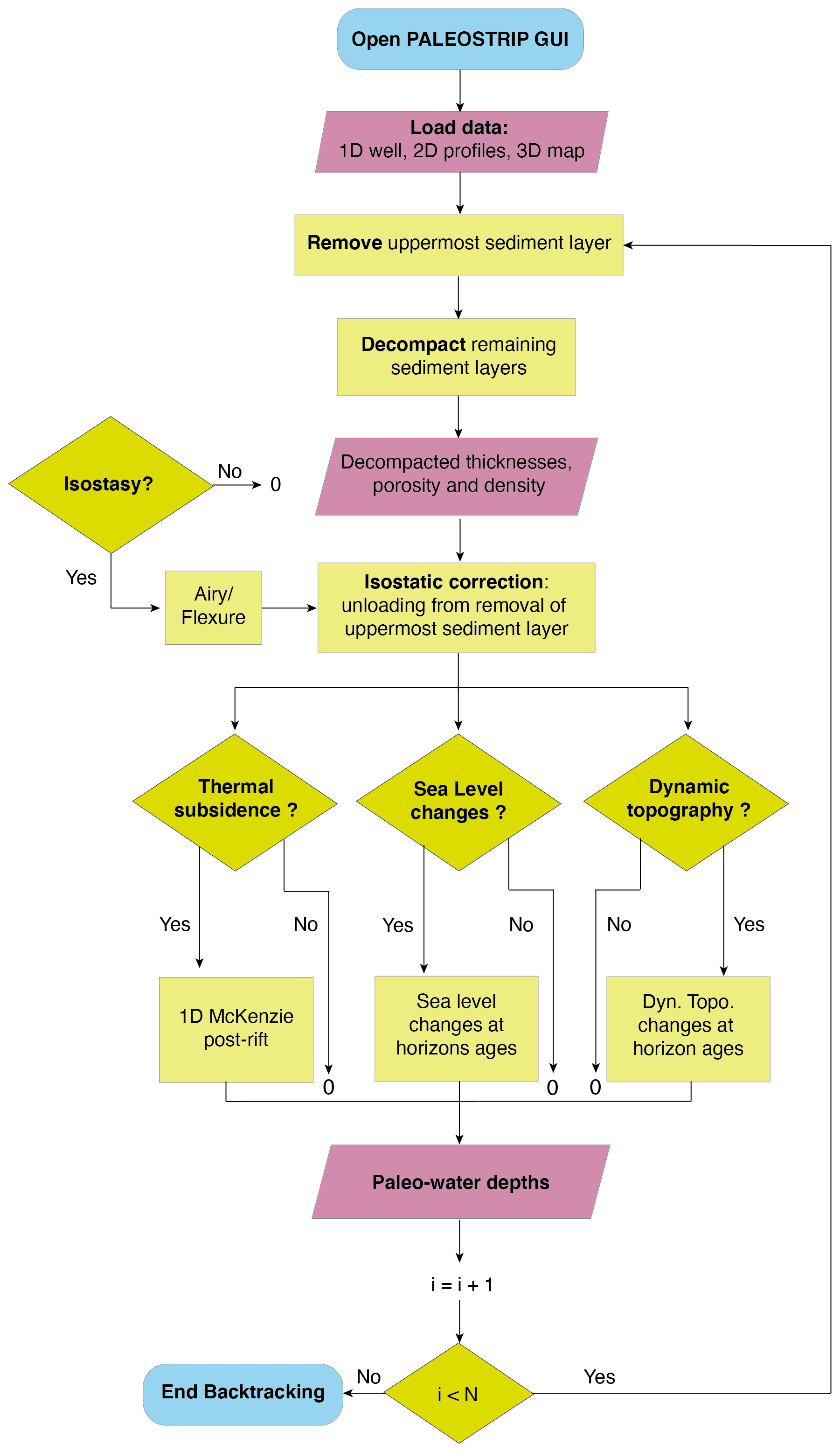
Figure 3Workflow of the code implemented in PALEOSTRIP illustrating the various steps of computation according to selected options in the GUI. N sediment layers are decompacted during the backtracking procedure. Smooth blue rectangles correspond to the start and end of the backtracking run. Light red parallelograms indicate input and output data. Light green rectangles are intermediate steps in the backtracking computation. Green diamonds correspond to options selected by the user in the GUI. If isostasy, thermal subsidence, sea level changes, or dynamic topography are switched off, the corresponding correction equals zero.
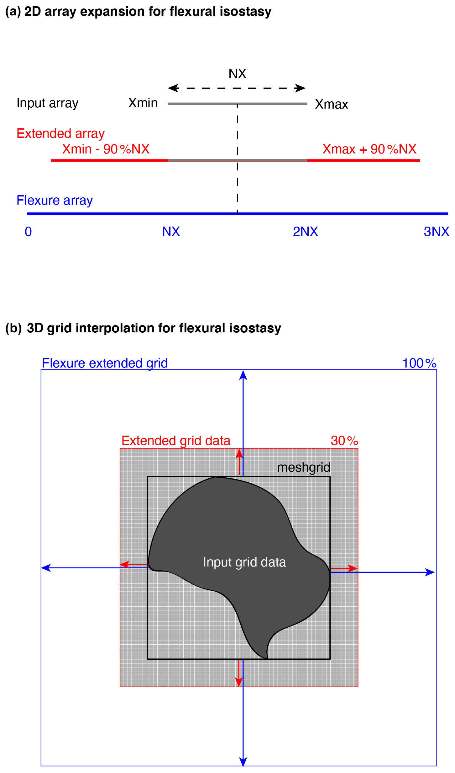
Figure 4The 2D and 3D domain expansions for computation of flexural isostasy. (a) In the case of 2D vertical sections, input data are extended with the edge values for 90 % of the initial total array length (NX). This extended array is placed at the centre of a null array that is 3 times larger than the initial input data array. (b) In the case of 3D maps, input data are extrapolated with a nearest neighbour algorithm on a mesh grid (black) to obtain a structured squared grid if the initial data are given on an irregular polygon. This mesh grid is extended by 30 % on all edges (red) and is placed at the centre of a grid twice as large as the mesh grid obtained from initial input data (blue).
During its evolution, a submarine continental margin can experience various processes that modify its morphology. For example, a rifted basin can form in response to plate tectonics displacement and/or erosion that shapes the basic structure of the margin. Surface erosion from the hinterland can supply the margin with sediments that fill morphological depressions if the accommodation space is large enough. The accommodation space depends on initial conditions, on the tectonics, and on the thermal subsidence of the continental margin, i.e. the lithosphere and asthenosphere cooling during and after the rifting that leads to a deepening of the margin over time. Eustatic and regional sea level changes modulate the available accommodation space and the distance from the sediment sources. To reconstruct the past subsidence history of a continental margin at a given time, all those processes have to be accounted for and corrected in a procedure called “backstripping” (Steckler and Watts, 1978). Backstripping consists of decompacting and removing sediment layers iteratively back in time to reconstruct the past tectonic subsidence history of a basin or a margin (Fig. 2):
where the first term of the right-hand side corresponds to the isostatic compensation (ρs sediment density, ρm mantle density, ρw seawater density) of the ith sediment layer thickness S(i) accumulated on the basement, WD(i) is the paleo-water depth of the ith layer, and the last term of the equation corresponds to the water load correction due to sea level variations (ΔSL) at time of the ith layer. This equation solves the time evolution of total subsidence Z(i) of the basement, and WD needs to be provided for each i layer to solve the equation. Conversely, in cases where the focus is on reconstructing time-varying paleo-water depths WD(i), the procedure is called “backtracking”, and a total subsidence Z(i) time evolution needs to be provided as input to the equation:
PALEOSTRIP is a backtracking software and is designed to reconstruct paleo-water depths given a provided subsidence history.
The equations above are the original backstripping and backtracking equations developed by Steckler and Watts (1978) and are explained therein in major detail. Over the past few decades, it has also been found that mantle convection generates changes in the regional topography, i.e. so-called “dynamic topography” (Müller et al., 2018a). Paleo-water depth needs to be corrected for dynamic topography changes ΔDynT(i) causing uplift or subsidence of the topography and bathymetry:
In this equation, the second and third terms on the right-hand side have been written accounting for Airy local isostatic compensation. However, PALEOSTRIP also makes use of 2D and 3D flexural isostasy (see Sect. 3.2). In this case, the second and third terms on the right-hand side of the equation represent the depth correction due to the flexural response to unloading of sediment during backtracking and to water loading or unloading due to sea level changes.
In the following, we explain how each term of Eq. (3) is treated within PALEOSTRIP. Most of the equations reported below are taken from Allen and Allen (2013) if not otherwise specified. The various aspects of the backtracking procedure are explained as part of the PALEOSTRIP workflow (Fig. 3).
Note that the physics implemented do not allow for the treatment of oceanic crust in this version. This can be done by adding a few more options in the GUI, mainly for thermal subsidence (e.g. Müller et al., 2018b). This can be easily implemented.
3.1 Decompaction
The total sediment thickness S accumulated at a given time can be obtained by reconstructing its compaction history. Eroded sediments are transported to the margin deposit and accumulate wherever the accommodation space allows for it. Accumulated sediments compact over time under loading, e.g. by overlying sediments. Therefore, to reconstruct the paleo-architecture of a continental margin at a given time, the sediment layers of a margin are stripped off sequentially, and the remaining underlying sediments need to be gradually decompacted. Decompaction is thus central to backstripping and backtracking.
Compaction or decompaction of sediments both imply a change in total volume Vtotal of deposited sediments; this is mostly caused by changes in the porosity of sediments and (to a lesser extent) changes in sediment compression. In submarine environments, sediments are saturated by water, and their compaction implies a decrease in pore fluid pressure via expelling of the water out of the sediment layers. Conversely, decompaction involves an increase in the pore fluid pressure by injecting water within the compacted sediments. The decompaction process consists of calculating the changes in porosity of the various sediment layers to determine the amount of water that was contained in the sediments at the time of their deposition based on their lithology. The depth of the decompacted sediment layers is recalculated on the basis of those porosity changes. Laboratory experiments have determined that for large depths, the evolution of porosity can be described by an exponential relationship rather than by a linear empirical equation:
where ϕ0 corresponds to deposition porosity at the seafloor (or at surface if emerged), c is the exponential slope decay coefficient (also referred to here as the compaction coefficient) depending on the lithology expressed in 1 km−1, and z is depth in kilometres. This empirical equation implies that ϕ0 is decreased by the factor of at the depth of km.
In general, the mass of the total sediment column at a given time does not change: in submarine environments the water that is expelled from the sediments is implicitly added to the water column above the underlying sediments during the compaction process. Thus, only the volume of the sediment layers Vtotal changes due to water volume changes Vw, which allows for the integration of the porosity Eq. (4). Considering a unit's cross-sectional area, the thickness of water WT to be added to the compacted sediment volume in order to decompact it is given by the following equation:
which upon integration gives
where and are the newly decompacted depths of zi and zi+1. Because the volume of sediment grains Vsed remains unchanged, the integrated compacted sediment thickness Sdt between two given depths, considering a unit's cross-sectional area, can be written as follows:
Based on the fact that , the decompacted depths z′(i) for a unit's cross-sectional area can be inferred, and the final decompaction equation is given by the following equation:
PALEOSTRIP solves this equation iteratively (starting with and then the further iterations) until convergence is reached. Lithological parameters, i.e. the decompaction coefficient c and the depositional surface porosity ϕ0, are prescribed in the user-provided parameter files (see Sect. 6).
3.2 Isostatic correction
Sediments load the basement of the continental margin and cause a local and regional subsidence during accumulation. Water also loads the basement due to eustatic sea level variations, leading to changes in the water depth WD that are also caused by ocean bottom subsidence and/or uplift through time. During the decompaction, the newly computed decompacted depths of the remaining sediment layers also need to be adjusted to account for the changes in their porosity and thus their density due to the presence of water filling the pores. For each sediment layer, the porosity ρds(i) of the decompacted thickness Sd(i) of the ith sediment layer is
and the decompacted sediment bulk density ρds(i) of the ith sediment layer is given by
At each time step, the removal of the top layer causes the decompaction of the underlying sediment layers.
Removed sediment layers are substituted with seawater. Unloading causes an isostatic compensation that can be calculated by using different isostatic methods. In PALEOSTRIP, two methods are implemented.
3.2.1 Airy local compensation
The Airy local compensation is the most used isostatic method in backstripping and backtracking. It involves a local depth compensation Zairy(i) for which the rocks and sediments and the underlying asthenosphere are considered to be in hydrostatic equilibrium:
This method implies that the weight of the sediments in a given grid point does not impact the adjacent points. Therefore, in the case of a 2D transect or a 3D map, grid points are independent of each other. This is of course not realistic, and the Airy local compensation preferably should be applied to the decompaction of wells only (Roberts et al., 1998).
3.2.2 Flexural compensation
When considering a wider area, i.e. decompacting a 2D transect or a 3D basin, a flexural compensation is required because a surface load tends to influence its surroundings. An Airy local compensation would not capture this effect and thus would overestimate the isostatic correction to be applied during the backstripping or backtracking (Roberts et al., 1998). Flexural compensation is based on the flexural strength of the lithosphere that is defined by its flexural rigidity D (in N m):
where E corresponds to the Young modulus (N m−2), Te is the effective elastic thickness of the lithosphere (m), and ν is the Poisson ratio. Total 1D flexure of the lithosphere for a line load on an infinite plate is given by the general analytical solution (Turcotte and Schubert, 2002):
and its 2D expression
where w is the deflection of the lithosphere (m), g is the gravity acceleration (m s−2), q(x,y) is the vertical load (N m−2) applied to the lithosphere, and x and y are the coordinates in the horizontal plane. In this equation, downward-deflected lithosphere is substituted with seawater ρw. The load q(x,y) (in N m−2) associated with each ith sediment layer is calculated as follows:
In PALEOSTRIP, 2D and 3D finite difference versions of Eqs. (13) and (14) have been implemented (e.g. Eqs. 9 and 10 in Wickert, 2016). They are based on Chapman (2015) flex2d and Cardozo (2009) flex3dv MATLAB codes that have been adapted to PALEOSTRIP needs. flex3dv routine is available at http://www.ux.uis.no/~nestor/Public/flex3dv.zip (last access: August 2021), and flex2d is available at https://www.jaychapman.org/matlab-programs.html (last access: August 2021). By means of a finite difference scheme, flexure can be computed by mean of an analytical solution (e.g. gflex, Wickert, 2016), whereas other numerical methods use the superposition of local solutions to point loads in the wavenumber domain (e.g. Green's functions, TAFI v1.0, Jha et al., 2017) or in the spectral domain (Wienecke et al., 2007), for example. These use biharmonic equation for plate flexure with uniform elastic properties. Approaches using the convolution method also allow the use of spatially variable elastic properties (e.g. Braitenberg et al., 2003, 2002). A file of spatially variable Te can be provided through the GUI (Fig. 1a, bottom). A spatially uniform Te can also be prescribed directly from the GUI. All other parameters involved in the flexural or Airy isostasy can be modified from the GUI (density constants, Poisson ratio, and Young modulus).
3.3 Thermal subsidence
Thermal subsidence corresponds to a vertical contraction of the lithosphere. During a rifting phase, as a first step, the lithosphere stretches apart and thins, which causes a net increase in heat outflow towards the surface due to the upwelling of the underlying asthenosphere. The stretching is generally not uniform, but reconstructions of past stretching processes require knowledge about plate tectonic strain rates (e.g. Müller et al., 2019), which is beyond the scope of our software. The first step is called “initial” subsidence. In the second step, the “thermal subsidence” occurs; i.e. the stretched lithosphere constricts due to cooling. To account for those effects during backstripping, PALEOSTRIP adopts the 1D-thermal subsidence model from McKenzie (1978) that assumes an instantaneous stretching (syn-rift) and a single rifting phase. The initial subsidence Zinit is given by
where TIL and TIC are the initial lithospheric and crustal thicknesses at the beginning of rifting, β is the stretching factor, αv is the coefficient of thermal expansion, ρc is the crustal density, and ρm is the mantle density. In this equation, the subsidence is isostatically compensated by water (ρw) using the Airy local compensation. This 1D instantaneous model can be improved by adopting a time-evolving approach to the extension, for example that of Jarvis and McKenzie (1980). However, comparison between Jarvis and McKenzie (1980) and McKenzie (1978) revealed that the two models show no or only little discrepancy if the duration of extension, given the time required to extend it by a factor of β, is about Myr if β≤2 or Myr if β≥2 (Jarvis and McKenzie, 1980). During the second step, the thermal subsidence occurs after the end of rifting (post-rift) and accounts for the vertical thermal conduction, which takes the shape of an exponential function decaying with time:
where t corresponds to the time elapsed since the end of rifting expressed in seconds (e.g. time of backtracked horizon = 14 Ma; age of the end of rifting = 76 Ma; and ).
where κ is the thermal diffusivity. The total thermal subsidence is given by
In PALEOSTRIP, during the backtracking procedure, paleo-water depths are corrected by removing the increment of thermal subsidence between each time step and present-day. This is because backtracking is an iterative process departing from a known state, i.e. present day. Because Zinit is constant in time it cancels out, and the thermal subsidence correction is given by
and thus,
where t varies from present to past in this equation following backstripping procedure, i.e. t is an age older than present day (0). ΔZtot_thermal is thus positive, with Zthermal being larger for younger times, i.e. a larger time is elapsed since the end of rifting.
Note that by applying the 1D model from McKenzie (1978) to 2D transects and 3D maps, it is assumed that no horizontal heat advection occurs. Almost all parameters involved in the thermal subsidence can be modified (age of end of rifting, TIL and TIC, αv, κ) from the GUI tab interface (Fig. 1b). The stretching factor β can be formulated through several methods.
- (1)
By prescribing a constant and uniform β factor that will be used at each time step of backtracking to calculate the thermal subsidence.
- (2)
By linearly interpolating (in the x direction for 3D maps) between two prescribed constant and uniform stretching factors, β1 and β2
- (3)
By inputting a user-based constant but spatially variable β factor in one direction (x grid) to compute spatially variable thermal subsidence for a 2D transect or by inputting a 2D (x,y grid) file to compute spatially variable thermal subsidence for 3D maps.
3.4 Sea Level correction
On long timescales, sea level has been varying with time due to plate tectonics changing the dimensions of ocean basins (e.g. Müller et al., 2018a) and, on shorter timescales, due to continental ice storage within ice sheets, ice caps, and glaciers during cold periods, as was the case, e.g. during the second half of the Cenozoic (the last 34 Myr, e.g. Miller et al., 2020). Classically, only eustatic sea level changes have been considered for correcting the subsidence or the paleo-water depth. For the last 34 Myr, eustatic sea level is usually defined relative to the present-day total ocean area (362.15×10⁶ km2) because it is assumed that this area evolved only a little and not enough to significantly alter this number. For time periods older than that, eustatic sea level changes have to be expressed according to the ocean area of the time. Considering only eustatic sea level changes results in highly approximated ice sheet growth and decay, leading to sea level variations of growing amplitude over the past 34 Myr (e.g. Miller et al., 2020). The variations induced by glaciations have much shorter timescales, i.e. 10–105 years, compared with those induced by plate tectonics (105–106 years). Associated sea level changes are not spatially uniform and induce changes in the Earth's gravity field (e.g. Tamisiea et al., 2001), and regional self-gravitating sea level changes can substantially vary from eustasy (e.g. Tamisiea et al., 2001; Clark et al., 2002; Milne and Mitrovica, 2008).
In PALEOSTRIP, sea level (SL, in m) is corrected the same way as thermal subsidence:
where t varies from present to past in this equation following a backtracking procedure, i.e., t is an age older than present day (0). ΔSL is expressed relative to present, and it can therefore assume positive or negative values, i.e. induce an uplift or a subsidence. Most of the sea level variation time series found in the literature already correspond to variations relative to present, i.e. are already in the form of Eq. (22). Thus, in order to avoid confusion for the user, three different ways of correcting water depth with sea level changes have been implemented within PALEOSTRIP and can be managed through the GUI (Fig. 1c):
- (1)
by prescribing constant and uniform sea level correction ΔSL applied at each time step of the backtracking (e.g. correction at a time where sea level is lower by 100 m relative to present is prescribed as −100 in the GUI),
- (2)
by applying a spatially uniform but time-varying sea level correction based on time series from Haq et al. (1987) or from Miller et al. (2020) (implemented within PALEOSTRIP);
- (3)
by applying a user-provided time series or a constant in time but spatially varying map of sea level changes relative to present.
The last option allows us to prescribe sea level changes calculated with glacio-isostatic adjustment models (e.g. SELEN4 Spada and Melini, 2019) to account for regional self-gravitating effects of ice sheet growth and decay. ΔSL is used to compute the water load correction to adjust the water depth WD. In Eq. (3), water load due to sea level change is described based on Airy local compensation. In PALEOSTRIP, the water load due to sea level change is computed using the isostatic method previously selected to carry out decompaction (see Sect. 3.2). Note that if isostasy is deactivated, no water load correction is computed.
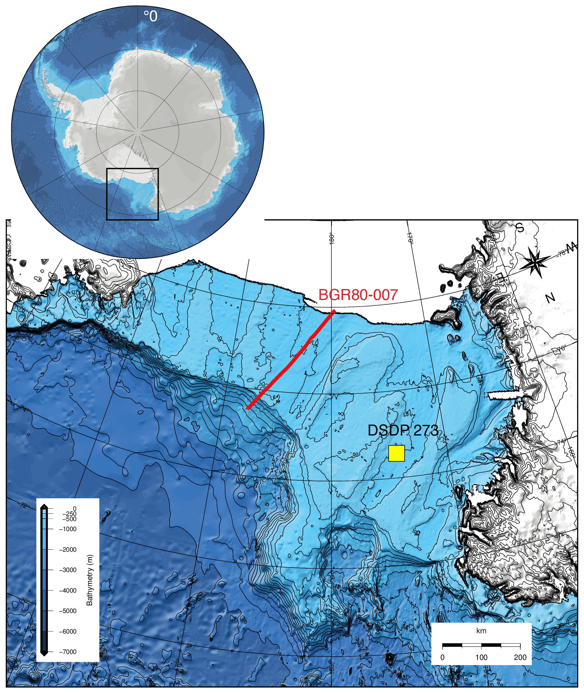
Figure 5Close-up of the Ross Sea bathymetry from IBCSO (Arndt et al., 2013) and its location in Antarctica. Most of the ice-free bathymetry is backtracked as shown in the case studies below. The BGR80-007 2D marine seismic transect used for validation is indicated with a red line, and the Deep Sea Drilling Project (DSDP) 273 site location, backtracked in the case studies below, is indicated with a yellow square.
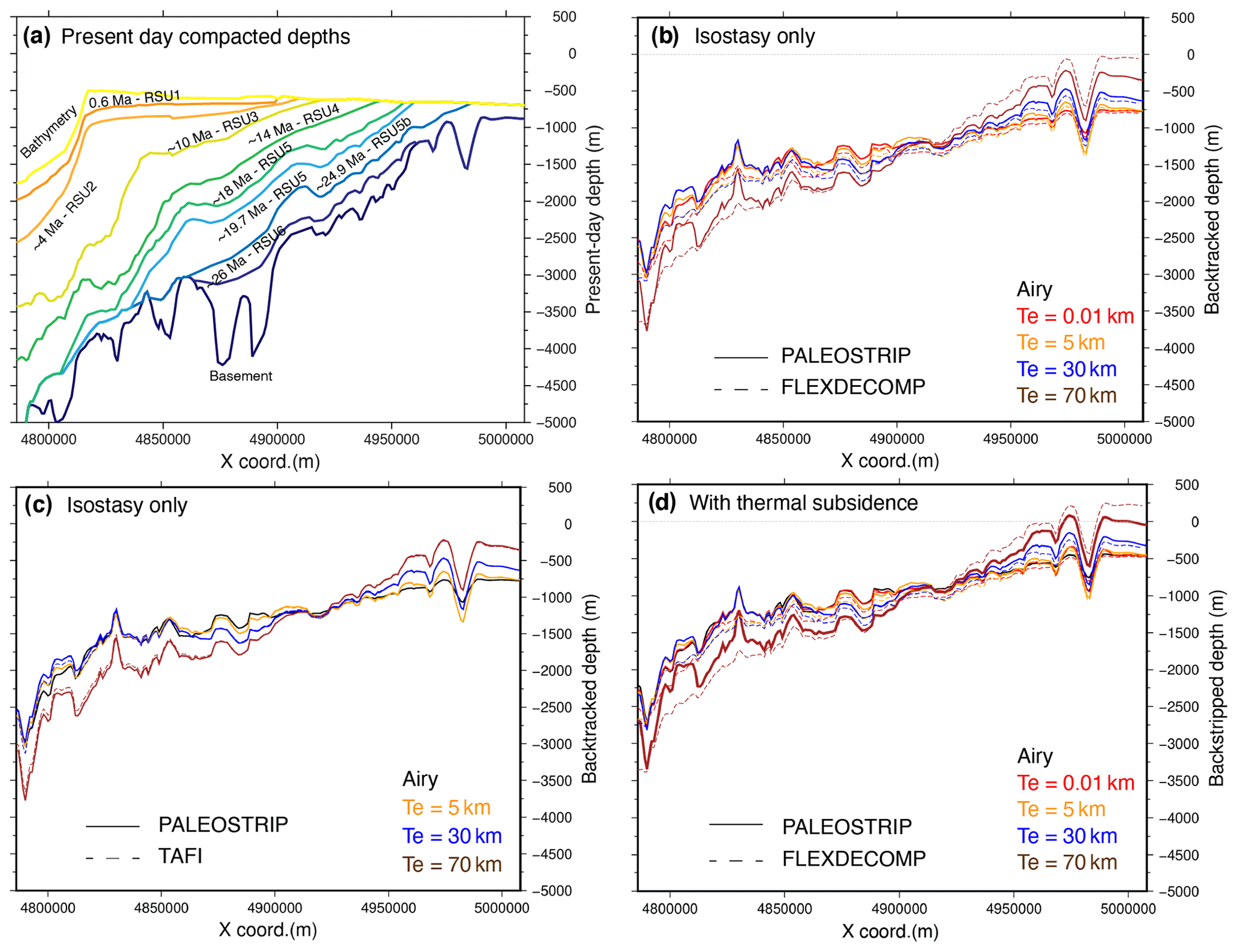
Figure 6The 2D transect BGR80-007 case study. (a) Input present-day compacted depths (m) of bathymetry (yellow) and the nine seismic unconformities, including the mid-Miocene Ross Sea Unconformity 4 (RSU4) and basement (thick blue line). Layout is from the PALEOSTRIP Plot GUI. Comparison of backtracked basement depths for different but spatially uniform lithospheric elastic thicknesses (Te): (b) between the PALEOSTRIP finite difference isostasy and the Flex-Decomp (Kusznir et al., 1995) fast Fourier transform (wavenumber-based) isostasy model; (c) between PALEOSTRIP finite difference isostasy and the TAFI (Jha et al., 2017) Green's function spectral isostasy model. Panel (d) is the same as (b) but accounts for the thermal subsidence correction using a rift age of 85 Myr and a uniform β of 2.
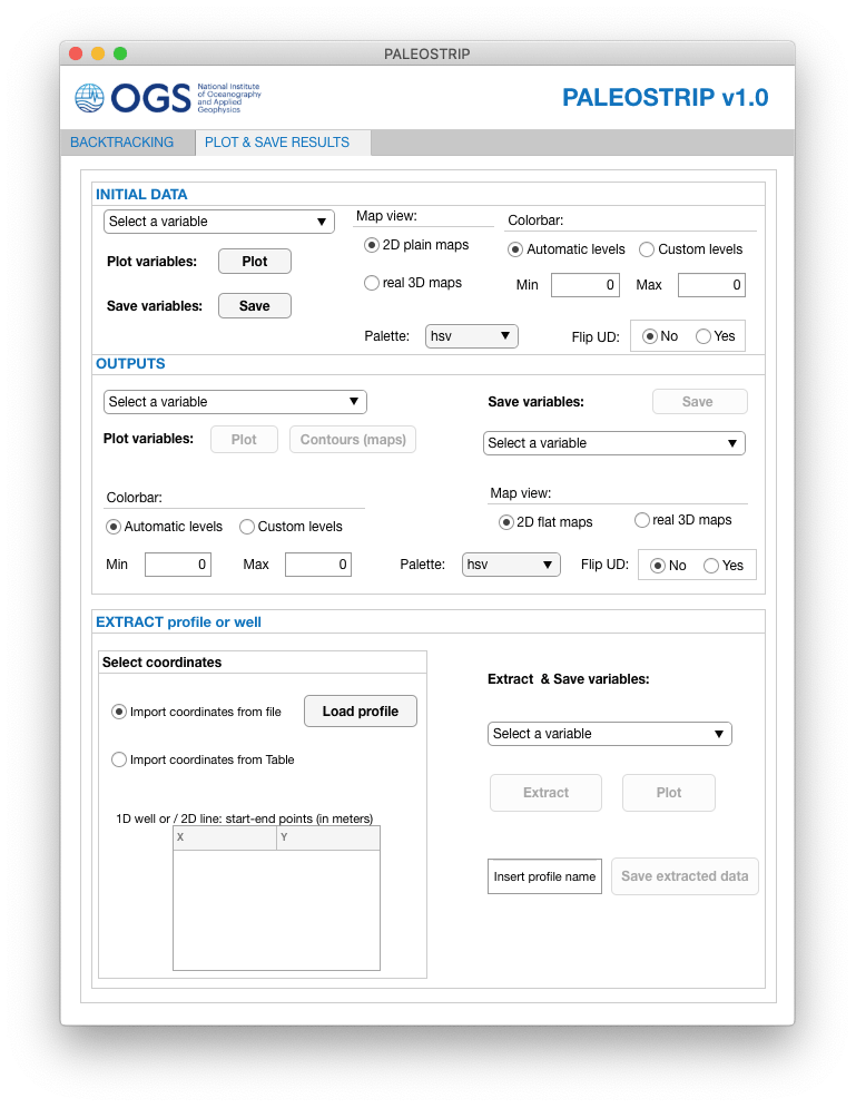
Figure 7PALEOSTRIP Application GUI plot and save results interface.
3.5 Dynamic topography
Mantle dynamics generate flows that cause time-varying surface topography and bathymetry deformations, which are called dynamic topography. The timescale at which the mantle flow produces dynamic topography that occurs at long wavelengths (≈5000 to 10 000 km Hoggard et al., 2016). The current mantle-driven dynamic topography was revealed by estimating the residual topography, obtained after removing the isostatic topography, which is generated by thickness and density contrasts within the lithosphere and the isostatic effect of the lithosphere calculated using seismic data compilations (e.g. Flament et al., 2013; Hoggard et al., 2016). Stratigraphic observations of continental margins revealed that the dynamic topography evolves quickly with time, potentially impacting long-term climate evolution (Hoggard et al., 2016). Austermann et al. (2017) showed that the magnitude of past interglacial sea level proxies partly results from dynamic topography, and they suggested correcting sea level proxies before inferring the relative contribution of past ice sheet to the sea level changes at that time. Furthermore, simulated Pliocene dynamic topography changes accounted for in Antarctic ice sheet simulations revealed that ice sheet stability is highly influenced by mantle dynamics that create or cancel pinning areas at the surface (Austermann et al., 2015). Thus past reconstructions of continental morphology and shallow margins should account for past evolution of dynamic topography. Müller et al. (2018a) recently provided time slices of reconstructed dynamic topography over the past 240 Myr, which constitutes a strong basis to calculate a dynamic topography correction.
PALEOSTRIP provides three ways to correct for dynamic topography changes through its GUI (Fig. 1d):
-
by prescribing a uniform and constant dynamic topography change relative to present day that will be applied to each time step of the backtracking procedure;
-
by using a user-based spatially uniform time series of dynamic topography changes relative to present;
-
by using user-based 2D maps of dynamic topography changes relative to present, e.g. Müller et al. (2018a) (note that Müller et al., 2018a, is not implemented within PALEOSTRIP); maps of dynamic topography are inputs to PALEOSTRIP and the user is free to use any reconstructions (note that inputs of dynamic topography require some pre-processing to be adjusted to the area of interest before being passed through the GUI).
The correction is calculated as for sea level changes (Eq. 22) as follows:
where t varies from present to past in this equation following backstripping procedure, i.e., t is an age older than present (0). ΔDynT is expressed relative to present, and since dynamic topography is not spatially uniform at a global level, it can therefore assume positive or negative values, i.e. induce an uplift or a subsidence.
3.6 Sediment erosion
Sediment erosion and depositions are the main processes involved in the building of continental margins. Present-day identified sedimentary units may not reflect the real number of sedimentary units at a given time in the past because some of the layers might have been eroded in the meantime. Erosion is identified within sediment cores as hiatus and as high-amplitude (sometimes truncational) reflectors within marine seismic profiles. During backstripping, one should move back eroded sediments to their presumed original locations (e.g. Paxman et al., 2019), which can be either within the backstripped area or outside the backstripped area. If eroded sediments are moved back in the backstripped area, then the total number of layers should be modified during the backward modelling process. The current version of PALEOSTRIP does not treat erosion and does not allow for the variation of the total number of sedimentary layers once they are input at the beginning of the procedure. A good description of how to handle erosion during backstripping is provided in Sect. 5.4 of Wangen (2010).
PALEOSTRIP handles 1D data (drill sites), 2D data (transects), and 3D data (grids). All calculations (except flexure) are performed on the grid or array of original input data. For 2D and 3D data, all input horizon depths have to be on the same grid or array (identical coordinates), and spacing along the X and Y directions must be constant. For 3D grids, spacing in the X direction can differ from spacing in the Y direction. For example, 2D transects must have horizons depths of the same length. The 3D maps can be provided as an irregular polygon, and all horizon depths must be provided on the same exact polygon (see examples in Sect. 6). At last, grid spacing dx and dy must be integers (e.g. dx=10 km and not dx=4.3 km).
4.1 2D data: vertical transects
Vertical transects imply that input data are provided along an horizontal direction X and a vertical direction (depth) Z. Due to the needs of flexure calculations, the original sediment loads array is extended (duplication of last values at both edges) to about 90 % of its length from both edges (Fig. 4a). The sediment loads are then placed at the centre of an expanded domain (3 times larger than the original array length) to avoid edge effects on flexure correction. After flexure calculation, the correction is extracted and relocated on the original array domain. All the other backtracking calculations occur on the original input array. Note that spatially variable lithospheric elastic thickness is also interpolated and extrapolated following this procedure.
4.2 3D data: maps
Maps imply that data are provided along the two horizontal directions, X and Y, and along the vertical direction, Z. Input data are read as scattered data and not as gridded data. This means that points are unstructured and are not written in a file following a classical NX×NY structure but are instead treated as independent single points. When data are treated as scattered this takes more computational time, but this also allows one to input either structured gridded data or irregular polygon data. This facilitates all computations and avoids unnecessary duplication of routines for 1D, 2D, or 3D cases. For the need of flexure, 3D data are interpolated (preserving their original horizontal resolution) on a regular rectangular grid. The original input grid is expanded (extrapolation of the last values from the edges) to about 30 % from all sides of the grid. The sediment loads are then placed at the centre of an expanded domain (twice as large as the original grid dimension) to avoid edge effects on flexure correction (Fig. 4b). After flexure calculation, the correction is extracted and relocated on the original grid domain. All the other backtracking calculations occur on the original input grid. Note that spatially variable lithospheric elastic thickness is also interpolated and extrapolated following this procedure.

Figure 8Backtracking steps for the western Ross Sea DSDP 273 well site. Present-day depths of the basement (black), Ross Sea unconformity 5 (blue), Ross Sea Unconformity 4A (orange), and bathymetry (brown) at the time of RSU4A (19 Ma), RSU5 (21 Ma), and at the time before glacial sediment deposition (>34 Ma). For each time step, two backtracking are shown, one accounting for Airy isostatic correction only and one accounting for Airy isostatic correction and thermal subsidence (dashed). Physical parameter values used are displayed in Table A1 in Appendix A.
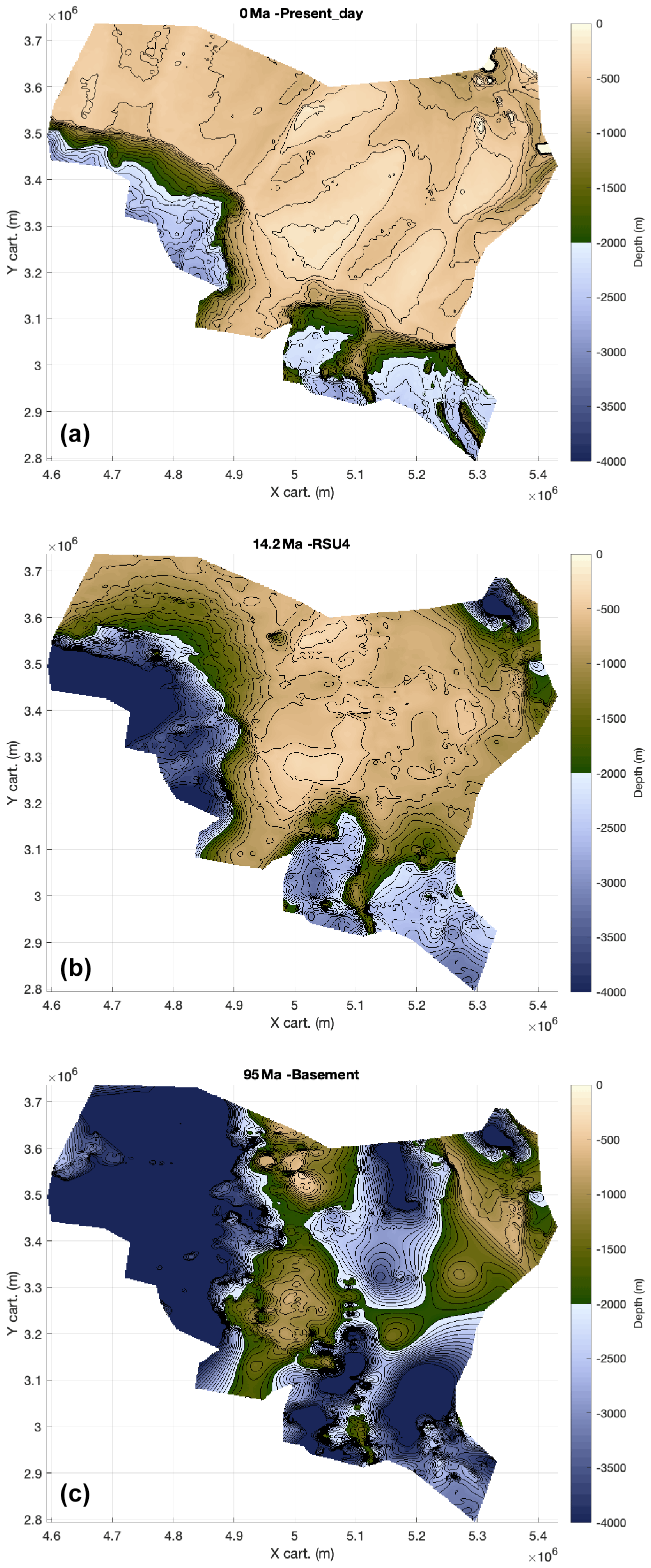
Figure 9Initial input present-day depths (m): (a) bathymetry, (b) mid-Miocene unconformity RSU4, and (c) basement both from ANTOSTRAT atlas (Brancolini et al., 1995). Layout is from the PALEOSTRIP plotting GUI; the colour scale is the default colour scale implemented within PALEOSTRIP. The colour scale has been saturated below −4000 m and above 200 m for this figure: the maximum depth of the basement reaches −10 km and would have largely damped the other bathymetric changes occurring at shallower depths in panels (a, b). The island located in the uppermost right corner is the only location with an elevation above sea level. Note that the colour scale is colour-blind friendly and is from Crameri et al. (2020). PALEOSTRIP has implemented 12 different colour scales, and 9 out of 12 are colour-blind friendly.
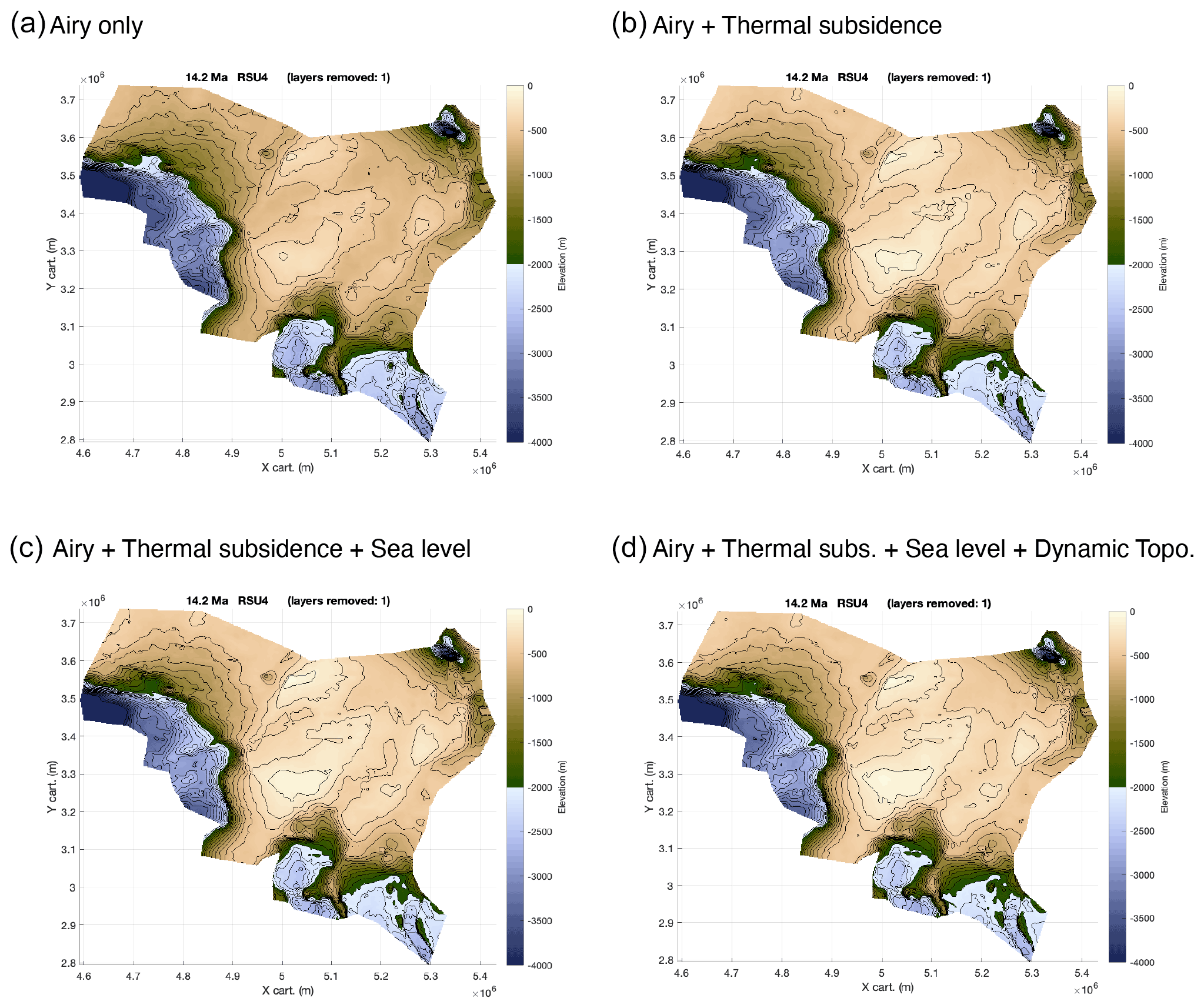
Figure 10Backtracked mid-Miocene bathymetries at about 14 Ma: (a) corrected only for Airy isostasy, (b) the same as (a) but including thermal subsidence correction with a spatially uniform β=2.1 and the end of rifting sets at 76 Ma, (c) the same as (b) but including eustatic sea level correction based on Miller et al. (2020) δ18O-derived reconstruction, (d) the same as (c) but including dynamic topography correction based on the Müller et al. (2018a) geodynamical model M1 (following Hochmuth et al., 2020). Layout is from the PALEOSTRIP plotting GUI; the colour scale is the default colour scale implemented within PALEOSTRIP and has been saturated below −4000 m and above 200 m for this figure. The island located in the uppermost right corner is the only location with an elevation above sea level. Note that the colour scale is colour-blind friendly and is from Crameri et al. (2020). PALEOSTRIP has implemented 12 different colour scales, and 9 out of 12 are colour-blind friendly. For all parameters used in these examples, see Table A1.
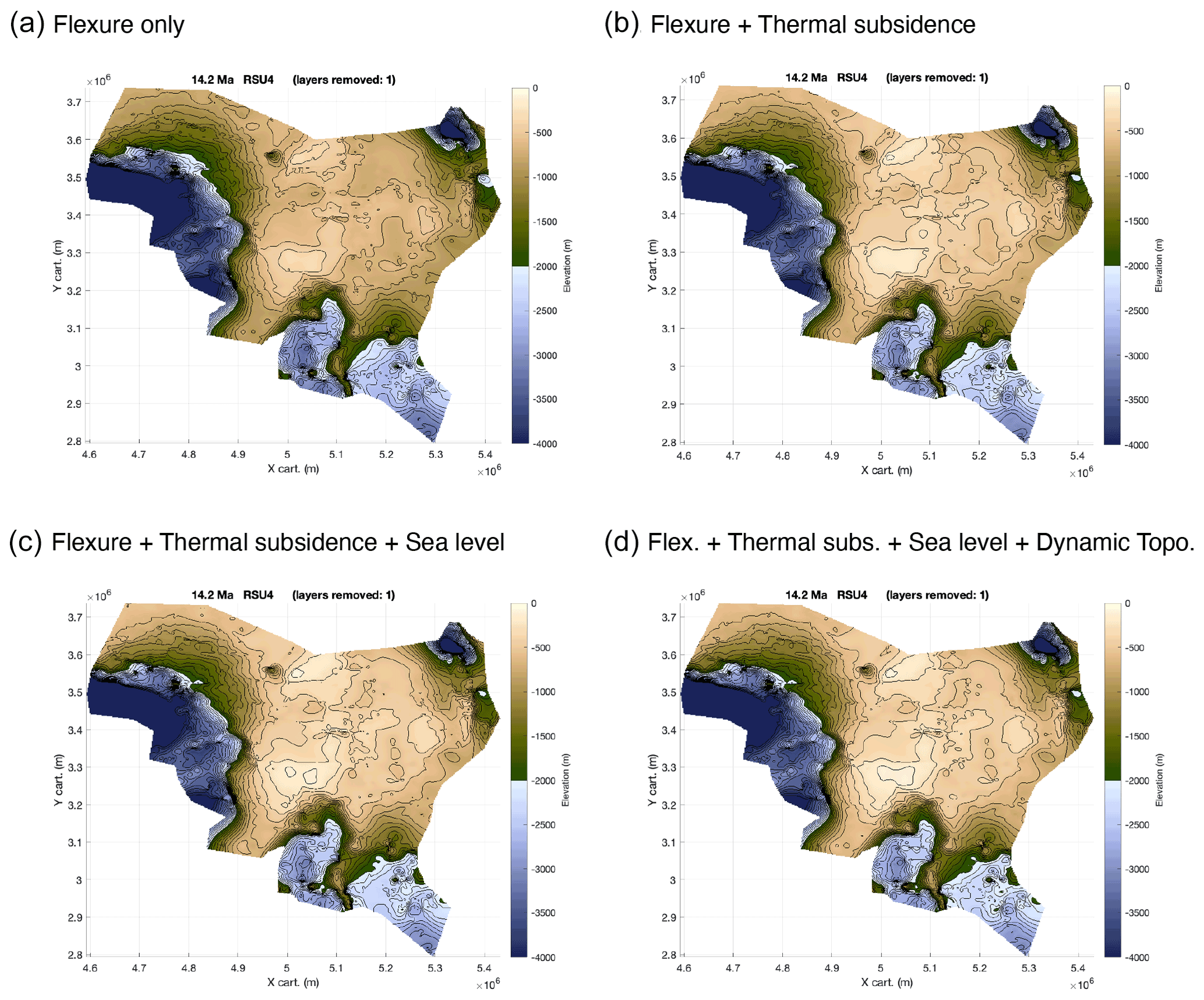
Figure 11Backtracked mid-Miocene bathymetries at about 14 Ma. The same as Fig. 10 but using flexural isostasy with spatially variable lithospheric effective elastic thickness from Chen et al. (2018). Layout is from the PALEOSTRIP plotting GUI; the colour scale is the default colour scale implemented within PALEOSTRIP and has been saturated below −4000 m and above 200 m for this figure. The island located in the uppermost right corner is the only location with elevation above sea level. Note that the colour scale is colour-blind friendly and is from Crameri et al. (2020). PALEOSTRIP has implemented 12 different colour scales, and 9 out of 12 are colour-blind friendly. For all parameters used in these examples, see Table A1 in Appendix A.
We backtrack a 2D transect with PALEOSTRIP and with Flex-Decomp (Kusznir et al., 1995) to validate the results. The transect used in the case study is a revised version of the one studied by De Santis et al. (1999): the BGR80-007 seismic profile. The transect BGR80-007 is composed of nine identified seismic stratigraphic unconformities. The transect is about 250 km long, is broadly oriented north–south, and is located in the eastern Ross Sea (Fig. 5). The set of initial data is composed of 10 files: the actual bathymetry of the Ross Sea and the present-day depth of the nine seismic unconformities, including the present-day depth of the basement below (Fig. 6a). Depths are related to present regional sea level.
The 11th file contains the lithological parameters of the layers to be decompacted, as well as other parameters needed by PALEOSTRIP, excluding present-day bathymetry: LAYER is the layer number (1 to N), from bottom to top), POROSITY is the deposition porosity (unitless), DEC CON (1 km−1) corresponds to the porosity decompaction coefficient, MAT DEN (kg m−3) corresponds to the compacted sediment density, AGE BASE (millions of years ago, Ma) is the age of horizons at the base of the layers, and NAME is the string name of horizons. The parameters are taken from the study of De Santis et al. (1999) and the lithological parameter file uses the following format:
NUMBER OF LAYERS =           9

LAYER POROSITY   DEC CON  MAT DEN    AGE BASE NAME
                 (1/KM)   (KG / M3)   (MA)

  1    0.4900    0.2700    2680.00    95.00   basement
  2    0.4500    0.4500    2680.00    26.00   rsu_6
  3    0.4500    0.4500    2680.00    24.90   rsu_5b
  4    0.4500    0.4500    2680.00    19.70   rsu_5a
  5    0.4500    0.4500    2680.00    18.00   rsu_5
  6    0.4500    0.4500    2680.00    14.20   rsu_4
  7    0.4500    0.4500    2680.00    10.00   rsu_3
  8    0.4500    0.4500    2680.00    4.00    rsu_2
  9    0.4500    0.4500    2680.00    0.60    rsu_1
To facilitate the comparison, thermal subsidence, sea level, and dynamic topography are switched off both in PALEOSTRIP and in Flex-Dedcomp. We compare the final backtracked depths of the basement using Airy local isostasy and flexural isostasy with different lithospheric elastic thicknesses (Fig. 6b). The match between PALEOSTRIP and Flex-Decomp is very good and persistent discrepancies (a few tens to hundreds of metres) are likely due to (1) the different ways of computing flexural isostasy in the spectral domain for Flex-Decomp and with finite difference for PALEOSTRIP, (2) re-interpolation of the load to a different resolution in Flex-Decomp (no reinterpolation in PALEOSTRIP), and (3) different extrapolation of the load outside of the original transect length to avoid edge effects on flexure. In PALEOSTRIP, the last point of the transects at both edges is duplicated to extend the original length of about 80 % at both sides (Fig. 4a). We also compare PALEOSTRIP backtracked results with those using the analytic solution from TAFI v1.0 (Jha et al., 2017) and implemented within PALEOSTRIP for the need of comparison (Fig. 6c). Similarly to the comparison with Flex-Decomp, we only account for isostasy and the other processes are switched off. Re-interpolation of the loads is performed by PALEOSTRIP in both cases. Comparison between PALEOSTRIP (finite difference scheme) and TAFI v1.0 reveal almost identical results.
Finally, we test the isostasy and thermal subsidence model by comparing those obtained by PALEOSTRIP and Flex-Decomp. De Santis et al. (1999) originally used Flex-Decomp with β=2, with the age of rifting set to 85 Ma and various lithospheric elastic thickness values to restore paleo-bathymetries. We use the same parameters on this revised transect in both Flex-Decomp and PALEOSTRIP. Match between PALEOSTRIP and Flex-Decomp is very good (Fig. 6d).
PALEOSTRIP GUI presents a plot and save interface to support each step of backtracking: the user can plot initial input data, backtracked data, and calculated intermediate variables relevant to the backtracking process and save them to ASCII files (Fig. 7). The user can also extract some 2D transects or 1D wells from 3D backtracked maps or 2D transects and plot and save them to ASCII files. In the following, we provide two case studies to illustrate the possibilities of PALEOSTRIP. Note that the physical parameters, sea level correction, or thermal-subsidence-related variables are not tuned since the aim of the examples is to illustrate the physics of PALEOSTRIP rather than to provide a realistic reconstruction of the paleo-bathymetries of this area.
Both the cases are taken from the continental margin in the western Pacific sector of Antarctica in the Ross Sea (Fig. 5). Sediment layers mostly accumulated after the main rifting phases that occurred in this area between 95 and 79 Ma (Stock and Cande, 2002; Decesari et al., 2007; Siddoway et al., 2004). Ross Sea stratigraphic data are currently being revised and differ from the ANTOSTRAT data (Brancolini et al., 1995) upon which the following 3D example is based. New reconstructed Ross Sea paleo-bathymetry using revised data will be the object of a specific contribution. ANTOSTRAT data have been recently used in pan-Antarctic reconstructions of past topographies and bathymetries (Paxman et al., 2019; Hochmuth et al., 2020).
6.1 Well (1D): Deep Sea Drilling Project (DSDP) site 273 – Ross Sea
In this example, we decompact the drilling site DSDP273 Hayes and Frakes (1975) from the western Ross Sea (Fig. 5). It has two main identified seismic unconformities above the basement. Lithological parameters are taken from De Santis et al. (1999), and the lithological parameters file (see Sect. 5) is as follows:
NUMBER OF LAYERS =           3

LAYER POROSITY  DEC CON   MAT DEN     AGE BASE NAME
                 (1/KM)   (KG / MC)   (MA)

  1    0.4500    0.2700    2680.00    95.00   basement
  2    0.4500    0.4500    2680.00    21.00   rsu_5
  3    0.4500    0.4500    2680.00    19.00   rsu_4a
Backtracking is performed using Airy local isostasy since flexure cannot be applied to 1D drilling sites. We also add thermal subsidence in order to illustrate the difference in backtracked depths of those unconformities (Fig. 8). The layout of Fig. 8 is not the layout of PALEOSTRIP, but the results have been assembled to highlight the impact of thermal subsidence on backtracked depths. As for 2D transects, all intermediate variables and input conditions can be plotted and saved.
6.2 Map (3D): ANTOSTRAT data
In this example we backtrack the depth of the mid-Miocene unconformity (14 Ma) across the Ross Sea from ANTOSTRAT atlas (Brancolini et al., 1995). The initial grid is an irregular polygon. The set of initial data is composed of three files: the actual bathymetry of the Ross Sea, the present-day depth of mid-Miocene unconformity, and the presumed present-day depth of the basement below (Fig. 9).
The fifth file contains the lithological parameters of the layers to be decompacted (see Sect. 5) and are taken from De Santis et al. (1999). The lithological parameters file is as follows:
NUMBER OF LAYERS =           2

LAYER  POROSITY  DEC CON   MAT DEN    AGE BASE  NAME
          (%)    (1/KM)   (KG / CC)   (MA)

  1    0.450     0.450     2680.0     95.000    Basement
  2    0.450     0.450     2680.0     14.200      RSU4
PALEOSTRIP is run several times to add one of the following components at a time: isostasy, thermal subsidence, sea level correction, and dynamic topography correction. Thanks to this approach, the user can perform ensembles of simulations to retrieve sound statistics of the model parameter space. Two series are shown, one using the Airy isostatic correction (Fig. 10) and the other using the flexural isostatic correction (Fig. 11). Paleo-bathymetry retrieved with flexural isostasy produces a quite different morphology from the one computed using Airy isostasy, as already observed by Roberts et al. (1998). Sea level and dynamic topography (Fig. A1b) corrections are not big enough to produce a significant change of the overall morphology. However, they matter for the bathymetric highs (especially the shallowest one), as a few tens of metres can uplift those highs above sea level. PALEOSTRIP allows the user to plot different variables amongst initial input data and computed quantities, such as isopach, density, porosity, or isostatic correction, allowing the user to check and separate the various processes required to perform a detailed analysis of their impact on the paleo-bathymetric reconstruction (Fig. A1).
PALEOSTRIP is one of the first examples of open-source 3D backtracking software. It can process paleo-bathymetries for 1D drilling sites, 2D transects, and 3D maps. It allows users to separate the various processes involved in the backtracking procedure. Thanks to this approach, the user can perform ensembles of simulations to retrieve sound statistics about the model parameter space. PALEOSTRIP has been designed to be modular to allow users to insert their own modifications. The code is documented, and thus implementation of new modules would only require minor work.
A1 Table of physical parameters
In all the examples provided, we used PALEOSTRIP default values automatically inserted within GUI (Table A1).
Miller et al. (2020)Müller et al. (2018b)
A2 Backtracked intermediate variables
Here we plot some of the intermediate physical variables calculated during the backtracking procedure and available for plotting through PALEOSTRIP GUI: sediment isopachs, decompacted density, decompacted porosity, isostatic correction, and dynamic topography (Fig. A1). Thermal subsidence is also available for plotting, but since we employ a spatially uniform β value here, thermal subsidence is consequently spatially uniform over the domain, and thus we do not display it.

Figure A1Example of input data and related backtracked sediment variables during the mid-Miocene: (a) spatially variable lithospheric elastic thickness (Chen et al., 2018) and (b) dynamic topography correction (Müller et al., 2018b). Both (a) and (b) are user-provided input to PALEOSTRIP. (c) Flexural isostatic correction calculated using (a). (d) Decompacted isopach (m). (e) Decompacted porosity (%). (f) Decompacted density (kg cm−3). Note that the colour scale is colour-blind friendly and is from Crameri et al. (2020). PALEOSTRIP has implemented 12 different colour scales, and 9 out of 12 are colour-blind friendly.
The version of the code and example data used in this paper are available on Zenodo https://doi.org/10.5281/zenodo.5092846 (Colleoni, 2021) or on GitHub https://github.com/flocolleoni/PALEOSTRIPv1.0 (last access: August 2021).
FC developed PALEOSTRIP code. LDS and RG provided input data for the case studies. All of the authors contributed to discussions about numerical developments of PALEOSTRIP and the writing of the manuscript.
The authors declare no competing interests.
Publisher's note: Copernicus Publications remains neutral with regard to jurisdictional claims in published maps and institutional affiliations.
We acknowledge Karsten Gohl and Katharina Hochmuth for their support in improving the software and the manuscript.
This work is supported by the PNRA national Italian projects: PNRA18_00002, “Onset of Antarctic Ice Sheet Vulnerability to Oceanic conditions (ANTIPODE)”, and PNRA16_00016, “West Antarctic Ice Sheet History from Slope Processes–Eastern Ross Sea (WHISPERS)”. It is also supported by the MAE bilateral Italy–US project US16GR04, “Global Sea Level rise and Antarctic Ice Sheet Stability predictions: guessing future by learning from past (GLSAISS)”.
This paper was edited by Andrew Wickert and reviewed by Karsten Gohl and Katharina Hochmuth.
Allen, P. A. and Allen, J. R.: Basin Analysis: Principles and Applications, Wiley, 2nd edn., 2013. a
Amadori, C., Garcia‐Castellanos, D., Toscani, G., Sternai, P., Fantoni, R., Ghielmi, M., and Di Giulio, A.: Restored topography of the Po Plain‐Northern Adriatic region during the Messinian base‐level drop – Implications for the physiography and compartmentalization of the palaeo‐Mediterranean basin, Basin Res., 30, 1247–1263, 2018. a
Arndt, J. E., Schenke, H. W., Jakobsson, M., Nitsche, F. O., Buys, G., Goleby, B., Rebesco, M., Bohoyo, F., Hong, J., Black, J., Greku, R., Udintsev, G., Barrios, F., Reynoso-Peralta, W., Taisei, M., and Wigley, R.: The International Bathymetric Chart of the Southern Ocean (IBCSO) Version 1.0 – A new bathymetric compilation covering circum-Antarctic waters, Geophys. Res. Lett., 40, 3111–3117, 2013. a
Austermann, J., Pollard, D., Mitrovica, J. X., Moucha, R., Forte, A. M., DeConto, R. M., Rowley, D. B., and Raymo, M. E.: The impact of dynamic topography change on Antarctic ice sheet stability during the mid-Pliocene warm period, Geology, 43, 927–930, 2015. a
Austermann, J., Mitrovica, J. X., Huybers, P., and Rovere, A.: Detection of a dynamic topography signal in last interglacial sea-level records, Science Advances, 3, e1700457, https://doi.org/10.1126/sciadv.1700457, 2017. a
Bracegirdle, T. J., Colleoni, F., Abram, N. J., Bertler, N. A., Dixon, D. A., England, M., Favier, V., Fogwill, C. J., Fyfe, J. C., Goodwin, I., Goosse, H., Hobbs, W., Jones, J. M., Keller, E. D., Khan, A. L., Phipps, S. J., Raphael, M. N., Russell, J., Sime, L., Thomas, E. R., van den Broeke, M. R., and Wainer, I.: Back to the future: Using long-term observational and paleo-proxy reconstructions to improve model projections of Antarctic climate, Geosciences, 9, 255, https://doi.org/10.3390/geosciences9060255, 2019. a
Braitenberg, C., Ebbing, J., and Götze, H.-J.: Inverse modelling of elastic thickness by convolution method–the Eastern Alps as a case example, Earth Planet. Sc. Lett., 202, 387–404, 2002. a
Braitenberg, C., Wang, Y., Fang, J., and Hsu, H.: Spatial variations of flexure parameters over the Tibet–Quinghai plateau, Earth Planet. Sc. Lett., 205, 211–224, 2003. a
Brancolini, G., Busetti, M., Marchetti, A., De Santis, L., Zanolla, C., and Cooper, A. K.: Seismic stratigraphic atlas of the Ross Sea, Antarctica, in: Geology and seismic stratigraphy of the Antarctic margin, Antarctic Research series, edited by: Cooper, A. K., Barker, P., and Brancolini, G., vol. 68, 271–286, 1995. a, b, c
Caesar, L., McCarthy, G., Thornalley, D., Cahill, N., and Rahmstorf, S.: Current Atlantic Meridional Overturning Circulation weakest in last millennium, Nat. Geosci., 14, 118–120, 2021. a
Cardozo, N.: flex3dv ©MATLAB software – http://www.ux.uis.no/%7Enestor/Public/flex3dv.zip (last access: August 2021), 2009. a
Celerier, B.: Paleobathymetry and geodynamic models for subsidence, Palaios, 3, 454–463, 1988. a
Chapman, J.: flex2d ©MATLAB software – https://www.jaychapman.org/matlab-programs.html (last access: August 2021), 2015. a
Chen, B., Haeger, C., Kaban, M. K., and Petrunin, A. G.: Variations of the effective elastic thickness reveal tectonic fragmentation of the Antarctic lithosphere, Tectonophysics, 746, 412–424, 2018. a, b
Clark, P. U., Mitrovica, J., Milne, G., and Tamisiea, M.: Sea-level fingerprinting as a direct test for the source of global meltwater pulse IA, Science, 295, 2438–2441, 2002. a
Colleoni, F.: flocolleoni/PALEOSTRIPv1.0: First release of PALEOSTRIP (v1.0.2), Zenodo, https://doi.org/10.5281/zenodo.5092846, 2021. a
Colleoni, F., De Santis, L., Montoli, E., Olivo, E., Sorlien, C. C., Bart, P. J., Gasson, E. G., Bergamasco, A., Sauli, C., Wardell, N., and Prato, S.: Past continental shelf evolution increased Antarctic ice sheet sensitivity to climatic conditions, Sci. Rep.-UK, 8, 1–12, 2018a. a
Colleoni, F., De Santis, L., Siddoway, C. S., Bergamasco, A., Golledge, N. R., Lohmann, G., Passchier, S., and Siegert, M. J.: Spatio-temporal variability of processes across Antarctic ice-bed–ocean interfaces, Nat. Commun., 9, 1–14, 2018b. a
Crameri, F., Shephard, G., and Heron, P.: The misuse of colour in science communication, Nat. Commun., 11, 5444, https://doi.org/10.1038/s41467-020-19160-7, 2020. a, b, c, d, e
De Santis, L., Prato, S., Brancolini, G., Lovo, M., and Torelli, L.: The Eastern Ross Sea continental shelf during the Cenozoic: implications for the West Antarctic ice sheet development, Global Planet. Change, 23, 173–196, 1999. a, b, c, d, e
Decesari, R. C., Wilson, D. S., Luyendyk, B. P., and Faulkner, M.: Cretaceous and Tertiary extension throughout the Ross Sea, Antarctica, in: Antarctica: A Keystone in a Changing World, in: Online Proceedings of the 0th ISAES, edited by: Cooper, A. and Raymond, C. R., Short Research Paper 098, ISAES, 2007. a
DeConto, R. M. and Pollard, D.: Contribution of Antarctica to past and future sea-level rise, Nature, 531, 591–597, 2016. a
Dressel, I., Scheck-Wenderoth, M., Cacace, M., Lewerenz, B., Götze, H.-J., and Reichert, C.: Reconstruction of the southwestern African continental margin by backward modeling, Mar. Petrol. Geol., 67, 544–555, 2015. a
Dressel, I., Scheck-Wenderoth, M., and Cacace, M.: Backward modelling of the subsidence evolution of the Colorado Basin, offshore Argentina and its relation to the evolution of the conjugate Orange Basin, offshore SW Africa, Tectonophysics, 716, 168–181, 2017. a
Eyring, V., Bony, S., Meehl, G. A., Senior, C. A., Stevens, B., Stouffer, R. J., and Taylor, K. E.: Overview of the Coupled Model Intercomparison Project Phase 6 (CMIP6) experimental design and organization, Geosci. Model Dev., 9, 1937–1958, https://doi.org/10.5194/gmd-9-1937-2016, 2016. a
Flament, N., Gurnis, M., and Müller, R. D.: A review of observations and models of dynamic topography, Lithosphere, 5, 189–210, 2013. a
Frigola, A., Prange, M., and Schulz, M.: Boundary conditions for the Middle Miocene Climate Transition (MMCT v1.0), Geosci. Model Dev., 11, 1607–1626, https://doi.org/10.5194/gmd-11-1607-2018, 2018. a
Golledge, N. R., Kowalewski, D. E., Naish, T. R., Levy, R. H., Fogwill, C. J., and Gasson, E. G.: The multi-millennial Antarctic commitment to future sea-level rise, Nature, 526, 421–425, 2015. a
Hansen, M. B., Scheck-Wenderoth, M., Hübscher, C., Lykke-Andersen, H., Dehghani, A., Hell, B., and Gajewski, D.: Basin evolution of the northern part of the northeast German Basin – Insights from a 3D structural model, Tectonophysics, 437, 1–16, 2007. a
Haq, B. U., Hardenbol, J., and Vail, P. R.: Chronology of fluctuating sea levels since the Triassic, Science, 235, 1156–1167, 1987. a
Hayes, D. and Frakes, L.: Initial Reports of the Deep Sea Drilling Project,Deep Sea Drilling Project, Texas AM University, 28 pp., 1975.. a
Haywood, A. M., Valdes, P. J., Aze, T., Barlow, N., Burke, A., Dolan, A. M., Von Der Heydt, A., Hill, D. J., Jamieson, S., Otto-Bliesner, B. L., Salzmann, U., Saupe, E., and Voss, J.: What can Palaeoclimate Modelling do for you?, Earth Systems and Environment, 3, 1–18, 2019. a
Herold, N., Seton, M., Müller, R., You, Y., and Huber, M.: Middle Miocene tectonic boundary conditions for use in climate models, Geochem. Geophys. Geosys., 9, Q10009, https://doi.org/10.1029/2008GC002046, 2008. a
Hochmuth, K., Gohl, K., Leitchenkov, G., Sauermilch, I., Whittaker, J. M., Uenzelmann-Neben, G., Davy, B., and De Santis, L.: The evolving paleobathymetry of the circum-Antarctic Southern Ocean since 34 Ma: A key to understanding past cryosphere-ocean developments, Geochem. Geophys. Geosys., 21, e2020GC009122, https://doi.org/10.1029/2020GC009122, 2020. a, b, c
Hoggard, M., White, N., and Al-Attar, D.: Global dynamic topography observations reveal limited influence of large-scale mantle flow, Nat. Geosci., 9, 456–463, 2016. a, b, c
Hölzel, M., Faber, R., and Wagreich, M.: DeCompactionTool: Software for subsidence analysis including statistical error quantification, Comput. Geosci., 34, 1454–1460, 2008. a
IPCC: Climate Change 2013: The Physical Science Basis, Contribution of Working Group I to the Fifth Assessment Report of the Intergovernmental Panel on Climate Change – Summary for policymakers, IPCC, Cambridge University Press, https://doi.org/10.1017/CBO9781107415324.004, 2013. a
IPCC: IPCC Special Report on the Ocean and Cryosphere in a Changing Climate: Summary for Policymakers, edited by: Pörtner, H.-O., Roberts, D. C., Masson-Delmotte, V., Zhai, P., Tignor, M., Poloczanska, E., Mintenbeck, K., Alegría, A., Nicolai, M., Okem, A., Petzold, J., Rama, B., and Weyer, N. M., IPCC, 2019. a
Jarvis, G. T. and McKenzie, D. P.: Sedimentary basin formation with finite extension rates, Earth Planet. Sc. Lett., 48, 42–52, 1980. a, b, c
Jha, S., Harry, D. L., and Schutt, D. L.: Toolbox for Analysis of Flexural Isostasy (TAFI) – A MATLAB toolbox for modeling flexural deformation of the lithosphere, Geosphere, 13, 1555–1565, 2017. a, b, c
Kirschner, J. P., Kominz, M. A., and Mwakanyamale, K. E.: Quantifying extension of passive margins: Implications for sea level change, Tectonics, 29, TC4006, https://doi.org/10.1029/2009TC002557, 2010. a
Kominz, M. A., Patterson, K., and Odette, D.: Lithology dependence of porosity in slope and deep marine sediments, J. Sediment. Res., 81, 730–742, 2011. a
Kusznir, N. J., Roberts, A. M., and Morley, C. K.: Forward and reverse modelling of rift basin formation, Geological Society, London, Special Publications, 80, 33–56, 1995. a, b, c
Lee, E. Y., Novotny, J., and Wagreich, M.: BasinVis 1.0: A MATLAB®-based program for sedimentary basin subsidence analysis and visualization, Comput. Geosci., 91, 119–127, 2016. a
Lee, E. Y., Novotny, J., and Wagreich, M.: Compaction trend estimation and applications to sedimentary basin reconstruction (BasinVis 2.0), Appl. Comput. Geosci., 5, 100015, 2020. a
MATLAB: version 9.9 (R2019b), The MathWorks Inc., Natick, Massachusetts, 2019. a
McKenzie, D.: Some remarks on the development of sedimentary basins, Earth Planet. Sc. Lett., 40, 25–32, 1978. a, b, c
Miller, K. G., Browning, J. V., Schmelz, W. J., Kopp, R. E., Mountain, G. S., and Wright, J. D.: Cenozoic sea-level and cryospheric evolution from deep-sea geochemical and continental margin records, Science advances, 6, eaaz1346, 2020. a, b, c, d, e
Milne, G. A. and Mitrovica, J. X.: Searching for eustasy in deglacial sea-level histories, Quaternary Sci. Rev., 27, 2292–2302, 2008. a
Müller, R., Hassan, R., Gurnis, M., Flament, N., and Williams, S. E.: Dynamic topography of passive continental margins and their hinterlands since the Cretaceous, Gondwana Res., 53, 225–251, 2018a. a, b, c, d, e, f, g
Müller, R. D., Cannon, J., Williams, S., and Dutkiewicz, A.: PyBacktrack 1.0: A tool for reconstructing paleobathymetry on oceanic and continental crust, Geochem. Geophys. Geosys., 19, 1898–1909, 2018b. a, b, c, d
Müller, R. D., Zahirovic, S., Williams, S. E., Cannon, J.and Seton, M., Bower, D. J., Tetley, M. G., Heine, C., Le Breton, E., Liu, S., Russell, S. H. J., Yang, T., Leonard, J., and Gurnis, M.: A global plate model including lithospheric deformation along major rifts and orogens since the Triassic, Tectonics, 38, 1884–1907, 2019. a
Noble, T., Rohling, E., Aitken, A. R. A., Bostock, H. C., Chase, Z., Gomez, N., Jong, L. M., King, M. A., Mackintosh, A. N., McCormack, F. S., McKay, R. M., Menviel, L., Phipps, S. J., Weber, M. E., Fogwill, C. J., Gayen, B., Golledge, N. R., Gwyther, D. E., Mc C. Hogg, A., Martos, Y. M., Pena-Molino, B., Roberts, J., van de Flierdt, T., and Williams, T.: The Sensitivity of the Antarctic Ice Sheet to a Changing Climate: Past, Present, and Future, Rev. Geophys., 58, e2019RG000663, https://doi.org/10.1029/2019RG000663, 2020. a
Otto-Bliesner, B. L., Jahn, A., Feng, R., Brady, E. C., Hu, A., and Löfverström, M.: Amplified North Atlantic warming in the late Pliocene by changes in Arctic gateways, Geophys. Res. Lett., 44, 957–964, 2017. a
Paxman, G. J., Jamieson, S. S., Hochmuth, K., Gohl, K., Bentley, M. J., Leitchenkov, G., and Ferraccioli, F.: Reconstructions of Antarctic topography since the Eocene–Oligocene boundary, Palaeogeogr. Palaeoecl., 535, 109346, https://doi.org/10.1016/j.palaeo.2019.109346, 2019. a, b
Paxman, G. J., Gasson, E. G., Jamieson, S. S., Bentley, M. J., and Ferraccioli, F.: Long-Term Increase in Antarctic Ice Sheet Vulnerability Driven by Bed Topography Evolution, Geophys. Res. Lett., 47, e2020GL090003, https://doi.org/10.1029/2020GL090003, 2020. a
Reerink, T. J., van de Berg, W. J., and van de Wal, R. S. W.: OBLIMAP 2.0: a fast climate modelice sheet model coupler including online embeddable mapping routines, Geosci. Model Dev., 9, 4111–4132, https://doi.org/10.5194/gmd-9-4111-2016, 2016. a
Riahi, K., van Vuuren, D. P., Kriegler, E., Edmonds, J., O'Neill, B. C., Fujimori, S., Bauer, N., Calvin, K., Dellink, R., Fricko, O., Lutz, W., Popp, A., Cuaresma, J. C., KC, S., Leimbach, M., Jiang, L., Kram, T., Rao, S., Emmerling, J., Ebi, K., Hasegawa, T., Havlik, P., Humpenöder, F., Da Silva, L. A., Smith, S., Stehfest, E., Bosetti, V., Eom, J., Gernaat, D., Masui, T., Rogelj, J., Strefler, J., Drouet, L., Krey, V., Luderer, G., Harmsen, M., Takahashi, K., Baumstark, L., Doelman, J. C., Kainuma, M., Klimont, Z., Marangoni, G., Lotze-Campen, H., Obersteiner, M., Tabeau, A., and Tavoni, M.: The Shared Socioeconomic Pathways and their energy, land use, and greenhouse gas emissions implications: An overview, Global Environ. Chang., 42, 153–168, https://doi.org/10.1016/j.gloenvcha.2016.05.009, 2017. a
Roberts, A., Corfield, R., Matthews, S., Kusznir, N., Hooper, R., and Gjeldvik, G.: Structural development and palaeobathymetry at the Norwegian Atlantic margin: revealed by 3D flexural-backstripping, in: 6th Petroleum Geology Conference: North West Europe and Global Perspectives, London, Abstracts, vol. 46, 2003. a, b
Roberts, A. M., Kusznir, N. J., Yielding, G., and Styles, P.: 2D flexural backstripping of extensional basins; the need for a sideways glance, Petrol. Geosci., 4, 327–338, 1998. a, b, c
Roberts, A. M., Alvey, A. D., and Kusznir, N. J.: Crustal structure and heat-flow history in the UK Rockall Basin, derived from backstripping and gravity-inversion analysis, Petrol. Geosci., 25, 131–150, 2019. a
Scheck, M., Bayer, U., and Lewerenz, B.: Salt redistribution during extension and inversion inferred from 3D backstripping, Tectonophysics, 373, 55–73, 2003. a
Sclater, J. G. and Christie, P. A.: Continental stretching: An explanation of the post-Mid-Cretaceous subsidence of the central North Sea Basin, J. Geophys. Res.-Sol. Ea., 85, 3711–3739, 1980. a
Siddoway, C. S., Baldwin, S. L., Fitzgerald, P. G., Fanning, C. M., and Luyendyk, B. P.: Ross Sea mylonites and the timing of intracontinental extension within the West Antarctic rift system, Geology, 32, 57–60, 2004. a
Smallwood, J. R.: Back-stripped 3D seismic data: A new tool applied to testing sill emplacement models, Petrol. Geosci., 15, 259–268, 2009. a
Spada, G. and Melini, D.: SELEN4 (SELEN version 4.0): a Fortran program for solving the gravitationally and topographically self-consistent sea-level equation in glacial isostatic adjustment modeling, Geosci. Model Dev., 12, 5055–5075, https://doi.org/10.5194/gmd-12-5055-2019, 2019. a
Steckler, M. and Watts, A.: Subsidence of the Atlantic-type continental margin off New York, Earth Planet. Sc. Lett., 41, 1–13, 1978. a, b, c
Steinberg, J., Roberts, A., Kusznir, N., Schafer, K., and Karcz, Z.: Crustal structure and post-rift evolution of the Levant Basin, Mar. Petrol. Geol., 96, 522–543, 2018. a
Stock, J. and Cande, S.: Tectonic history of Antarctic seafloor in the Australia-New Zealand-South Pacific sector: Implications for Antarctic continental tectonics, B. Roy. S. NZ, 35, 251–259, 2002. a
Straume, E. O., Gaina, C., Medvedev, S., and Nisancioglu, K. H.: Global Cenozoic Paleobathymetry with a focus on the Northern Hemisphere Oceanic Gateways, Gondwana Res., 86, 126–143, 2020. a, b
Tamisiea, M., Mitrovica, J., Milne, G., and Davis, J.: Global geoid and sea level changes due to present-day ice mass fluctuations, J. Geophys. Res.-Sol. Ea., 106, 30849–30863, 2001. a, b
Turcotte, D. L. and Schubert, G.: Geodynamics, Cambridge University Press, 2nd edn., https://doi.org/10.1017/CBO9780511807442, 2002. a
Wangen, M.: Physical Principles of Sedimentary Basin Analysis, Cambridge University Press, https://doi.org/10.1017/CBO9780511711824, 2010. a
Wickert, A. D.: Open-source modular solutions for flexural isostasy: gFlex v1.0, Geosci. Model Dev., 9, 997–1017, https://doi.org/10.5194/gmd-9-997-2016, 2016. a, b
Wienecke, S., Braitenberg, C., and Götze, H.-J.: A new analytical solution estimating the flexural rigidity in the Central Andes, Geophys. J. Int., 169, 789–794, 2007. a
Zhang, Y. G., Pagani, M., Liu, Z., Bohaty, S. M., and DeConto, R.: A 40-million-year history of atmospheric CO2, Philos. T. Roy. Soc. A, 371, 20130096, 2013. a
- Abstract
- Introduction
- Model framework and requirements
- PALEOSTRIP: backtracking and limitations
- PALEOSTRIP grid interpolation
- PALEOSTRIP validation
- Case study: example of the Ross Sea
- Conclusions
- Appendix A: Case studies: settings
- Code and data availability
- Author contributions
- Competing interests
- Disclaimer
- Acknowledgements
- Financial support
- Review statement
- References