the Creative Commons Attribution 4.0 License.
the Creative Commons Attribution 4.0 License.
 | 12 Aug 2021
WAP-1D-VAR v1.0: development and evaluation of a one-dimensional variational data assimilation model for the marine ecosystem along the West Antarctic Peninsula
Ya-Wei Luo
Hugh W. Ducklow
Oscar M. Schofield
Deborah K. Steinberg
Scott C. Doney
The West Antarctic Peninsula (WAP) is a rapidly warming region, with substantial ecological and biogeochemical responses to the observed change and variability for the past decades, revealed by multi-decadal observations from the Palmer Antarctica Long-Term Ecological Research (LTER) program. The wealth of these long-term observations provides an important resource for ecosystem modeling, but there has been a lack of focus on the development of numerical models that simulate time-evolving plankton dynamics over the austral growth season along the coastal WAP. Here, we introduce a one-dimensional variational data assimilation planktonic ecosystem model (i.e., the WAP-1D-VAR v1.0 model) equipped with a model parameter optimization scheme. We first demonstrate the modified and newly added model schemes to the pre-existing food web and biogeochemical components of the other ecosystem models that WAP-1D-VAR model was adapted from, including diagnostic sea-ice forcing and trophic interactions specific to the WAP region. We then present the results from model experiments where we assimilate 11 different data types from an example Palmer LTER growth season (October 2002–March 2003) directly related to corresponding model state variables and flows between these variables. The iterative data assimilation procedure reduces the misfits between observations and model results by 58 %, compared to before optimization, via an optimized set of 12 parameters out of a total of 72 free parameters. The optimized model results capture key WAP ecological features, such as blooms during seasonal sea-ice retreat, the lack of macronutrient limitation, and modeled variables and flows comparable to other studies in the WAP region, as well as several important ecosystem metrics. One exception is that the model slightly underestimates particle export flux, for which we discuss potential underlying reasons. The data assimilation scheme of the WAP-1D-VAR model enables the available observational data to constrain previously poorly understood processes, including the partitioning of primary production by different phytoplankton groups, the optimal chlorophyll-to-carbon ratio of the WAP phytoplankton community, and the partitioning of dissolved organic carbon pools with different lability. The WAP-1D-VAR model can be successfully employed to link the snapshots collected by the available data sets together to explain and understand the observed dynamics along the coastal WAP.
- Article
(10621 KB) - Full-text XML
-
Supplement
(263 KB) - BibTeX
- EndNote


The West Antarctic Peninsula (WAP) has experienced significant atmospheric and surface ocean warming since the 1950s, resulting in decreased winter sea-ice duration, the retreat of glaciers, and changes in upper-ocean dynamics (Clarke et al., 2009; Cook et al., 2005; Henley et al., 2019; King, 1994; Meredith and King, 2005; Stammerjohn et al., 2008; Vaughan et al., 2003, 2006; Whitehouse et al., 2008). These climate-driven changes propagate through marine food webs by affecting physiology of individual organisms and the whole communities (Ducklow et al., 2007). Long-term observational efforts through the Palmer Antarctica Long-Term Ecological Research program (LTER; since 1991) have demonstrated a range of ecological and biogeochemical responses to changing environments, including phytoplankton (Montes-Hugo et al., 2009; Saba et al., 2014; Schofield et al., 2017), marine heterotrophic bacteria (Bowman and Ducklow, 2015; Ducklow et al., 2012; Kim and Ducklow, 2016; Luria et al., 2014, 2017), nutrient drawdown (Kim et al., 2016), and micro- and macrozooplankton (Garzio and Steinberg, 2013; Steinberg et al., 2015; Thibodeau et al., 2019).
The wealth of Palmer LTER time-series observations provides an important resource for ecological and biogeochemical modeling, and different types of modeling approaches have been developed to explore the WAP responses to climate change and variability. For instance, an inverse modeling study estimated the steady-state dynamics of the WAP food web by deriving snapshots of flows among different plankton functional types and higher trophic levels (Sailley et al., 2013). However, there has been less focus on numerical ecosystem models that simulate time-evolving plankton dynamics over the full austral growth season along the coastal WAP. Numerical ecosystem models provide estimates of key rate processes for which observations have been less frequently or seldom made compared to frequently measured stocks and rates. Despite its strengths, constructing an ecosystem model is a challenge due to the lack of a priori knowledge on model parameter values and incomplete understanding of ecological processes that should be explicitly presented in the model structure (Ducklow et al., 2008; Murphy et al., 2012). Due to many observational studies, a more robust, yet still incomplete, data-based picture is emerging of WAP food-web interactions and ecosystem dynamics, which could guide a development of the WAP-specific numerical ecosystem model.
Here, we introduce a one-dimensional (1-D) variational data assimilation model specific to the coastal WAP (i.e., the WAP-1D-VAR v1.0 model) that we develop by adapting an existing biogeochemical–planktonic model of different ocean basins (Friedrichs, 2001; Friedrichs et al., 2006, 2007; Luo et al., 2010). The WAP-1D-VAR model is compared against the roughly semi-weekly biophysical observations over the austral growth season near Palmer Station on Anvers Island, Antarctica (64.77∘ S, 64.05∘ W). The field data record the seasonal variations in the initiation, peak, and termination of phytoplankton blooms and other biogeochemical processes modulated by variations in surface light, mixed layer depth, and sea-ice cover. In the present study, we (1) describe the structure and schemes of the WAP-1D-VAR model in great detail, (2) evaluate the model performance and robustness using a variety of quantitative metrics, and (3) discuss the model applicability with regard to capturing the key WAP ecological and biogeochemical features using the data from an example growth season.

Figure 1The WAP-1D-VAR v1.0 model is forced by five different physical forcing, denoted as a horizontal row across the top of the schematic of the ecosystem model. The ecosystem component incorporates 11 different prognostic state variables. Higher level and refractory dissolved organic matter (RDOM) are represented implicitly.
2.1 Model state variables
The WAP-1D-VAR v1.0 model (Fig. 1) is originally derived and modified from data-assimilative, ocean regional test-bed models of the Arabian Sea, the equatorial Pacific, and the Hawaii Ocean Time-series Station ALOHA (A Long-Term Oligotrophic Habitat Assessment) (Friedrichs, 2001; Friedrichs et al., 2006, 2007; Luo et al., 2010). The WAP-1D-VAR model simulates stocks and flows of C, N, and P through 11 different model prognostic state variables. The two size-fractionated phytoplankton compartments (i.e., diatoms and cryptophytes) and the two different zooplankton compartments (i.e., microzooplankton and krill) are separately simulated following the plankton functional types as in Sailley et al. (2013) and the observations of the phytoplankton community structure along the coastal WAP. Typically, the coastal WAP is associated with large phytoplankton accumulations dominated by large (>20 µm) diatoms, but nanoflagellates (<20 µm) or cryptophytes are also an important component of the food web (Schofield et al., 2017). Mixed flagellates, prasinophytes, and type-4 haptophytes are also found in the region, but we choose to model only diatoms and cryptophytes, in order to avoid too many free (optimizable) parameters associated with each phytoplankton group. The third most dominant species is mixed flagellate but little is known about these taxa in the region and these taxa generally exhibit low interannual variability (Schofield et al., 2017). Functional grazing relationships are defined in which diatoms are consumed by both krill (Euphausia superba) and microzooplankton (mostly ciliates and other protozoa), cryptophytes are consumed by microzooplankton, and microzooplankton are grazed by krill. Other abundant zooplankton taxa in the WAP, such as salps, pteropods, and copepods (Steinberg et al., 2015), are not explicitly simulated in the WAP-1D-VAR model, in part to limit the model complexity and in part because of the limited data constraints on these groups, especially feeding. Higher trophic levels are implicitly represented to close the model. The WAP-1D-VAR model allows for the partitioning between labile dissolved organic matter (LDOM) and semi-labile DOM (SDOM) such that the entire LDOM pool is available but only a limited portion of the SDOM is available for bacterial utilization to account for lower lability of SDOM. Refractory DOM (RDOM) is not explicitly modeled due to its much longer turnover time than labile and semi-labile pools, but some mass flows are included to RDOM from other prognostic model compartments, such as bacteria, krill, and SDOM, to account for loss terms for those state variables. Detritus represents an average particulate organic matter (POM) pool after removing living phytoplankton and bacterial biomass, and sinking of the detritus pool contributes to particle export flux. The WAP-1D-VAR model explicitly simulates NO3, NH4, and PO4 for inorganic (macro)nutrient compartments, but there is not a separate Fe model compartment or Fe uptake processes, given that even during the peak of the blooms iron is still measurable and iron limitation is absent or occurs only minimally and seasonally in the nearshore Palmer Station area (Carvalho et al., 2016; Sherrell et al., 2018).
2.2 Model equations
Here, we demonstrate key model processes that are either based on the existing schemes or built as new schemes for the coastal WAP region. The original model schemes are detailed in Supplementary Material of Luo et al. (2010). The WAP-1D-VAR v1.0 model simulates biological–physical model processes for a 1-D vertical water column, solving numerically for a discretized version of the time rate of change for each model state variable. For a generic tracer variable C, the time rate of change equation takes the form (Glover et al., 2011)
where z is the depth, w is the vertical velocity (the sum of water motion and gravitational particle sinking), Kz is the turbulent eddy diffusivity, and JC is the biological and biogeochemical net source and sink term for C (Appendix A Equations; Eqs. A42–A45, A82–A85, A138–A140, A164–A166, A193–A195, A199–A201, A205–A210, and A212–A214). The physical advection and mixing terms are discussed below in Sect. 2.3 and applied sequentially following the computation of the biological and biogeochemical terms JC using a constant time step of 1 h. The contributions of the source sink terms JC to the full time rate of change equations are constructed as a series of coupled ordinary differential equations, detailed in Appendix A (Sects. A1–A9), and solved using a second-order Runge–Kutta numerical integration scheme. The WAP-1D-VAR model simulates the dynamics of C, N, and P, but here we only focus on the presentation of the model C dynamics. The cellular molar (e.g., NC, PC) quota parameter values of most state variables are fixed (Table 1) and not submitted to the optimization and data assimilation procedure. To first order, most model physiological processes are affected by water temperature, including the maximum growth rates of phytoplankton, bacteria, and zooplankton and basal respiration rates of bacteria and zooplankton. The Arrhenius function is implemented to change these physiological rates as a function of water temperature (Eq. A1).
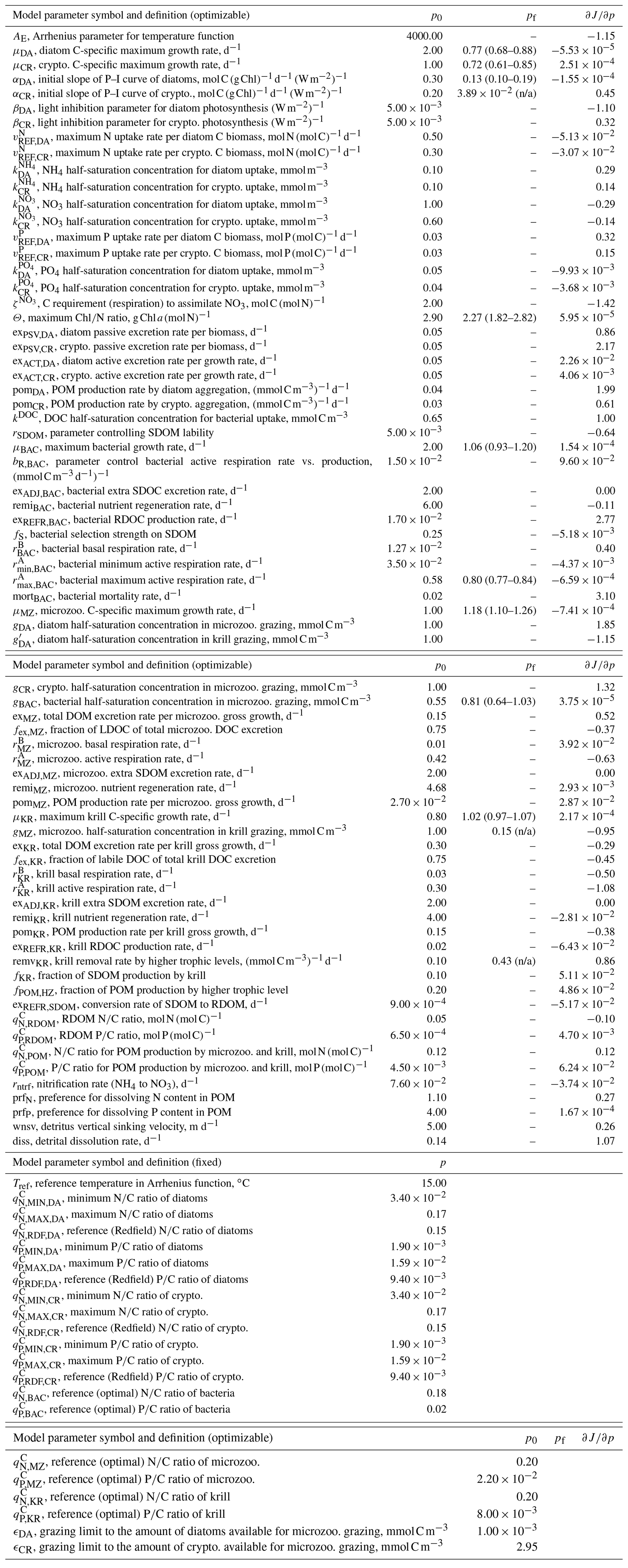
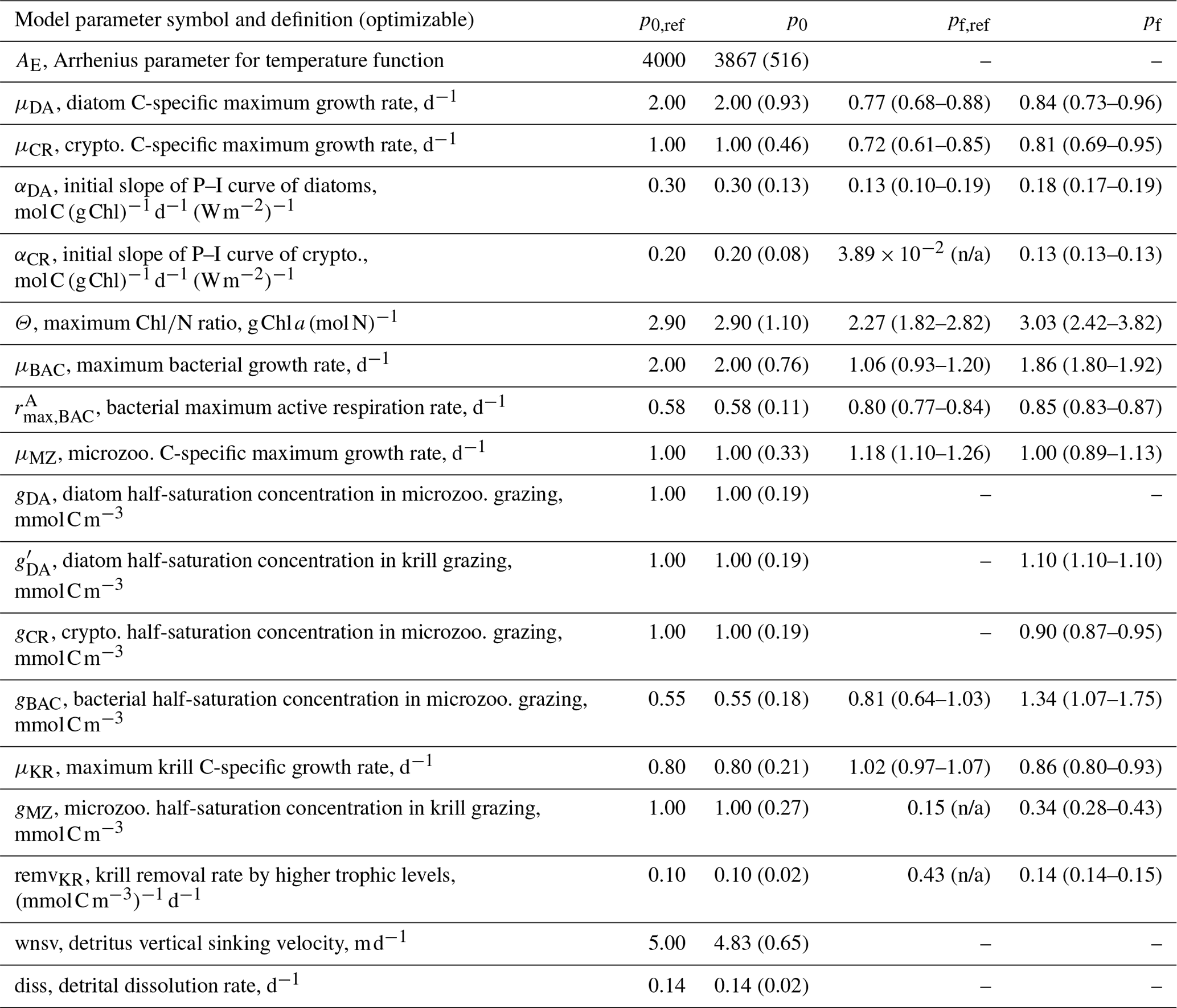
Table 1Summary of the model parameter symbol and definition, initial parameter values (p0) and optimized values (pf) for optimizable parameters, the cost function gradient with regard to the optimized parameter (), and prescribed values for fixed model parameters over the course of simulations. The parameter with “n/a” in the parentheses is an optimized parameter with a large relative uncertainty, while the parameter with values in the parentheses is a constrained parameter (optimized with a low relative uncertainty) with its upper and lower bounds. The uncertainties for these upper and lower bounds are calculated as , where pf is the value of the constrained parameter and σf is the square roots of diagonal elements of the inverse of the Hessian matrix. The cost function gradient with regard to the optimized parameter () after data assimilation is defined as where eΔp≈Δp for an infinitely small Δp.
The net change of phytoplankton (both diatoms and cryptophytes) C biomass is driven by gross growth, DOC excretion, particulate organic carbon (POC) production via aggregation, respiration, and grazing (Eqs. A42 and A82), the net change of their N and P biomass by gross growth, dissolved organic nitrogen (phosphorus) excretion, particulate organic nitrogen (phosphorus) production, and grazing (Eqs. A43–A44 and A83–A84). The net change of their chlorophyll a (Chl a) by gross growth, DOM excretion, and grazing (Eqs. A45 and A85). The WAP-1D-VAR model adapts a phytoplankton growth scheme with flexible stoichiometry, in which phytoplankton cells are allowed to accumulate and store more nutrients under light stress (Bertilsson et al., 2003; Droop, 1974, 1983; McCarthy, 1980). The phytoplankton C growth rate is limited by their cellular nutrient quota (Eqs. A2–A3 and A46–A47). Modified from Geider et al. (1998), phytoplankton nitrogen uptake decreases when their cellular NC quota is higher than their reference (Redfield) ratio but not limited when lower than their reference ratio (Eqs. A5, A9, A49, and A53). The nitrogen consumption completely ceases when the phytoplankton cellular quota reaches their maximum allowable ratios and is additionally limited by the ambient NO3 and NH4 concentrations with a Monod function (Eqs. A11–A12 and A55–A56). NH4 inhibition on NO3 uptake of phytoplankton is modeled by assigning lower compared to (Table 1). The inhibition term does not exist for PO4. The uptake scheme is similar for PO4 (Eqs. A14 and A58), but PO4 can be consumed in great excess of current needs (Armstrong, 2006). Such luxury uptake is modeled by assigning smaller maximum and minimum P quota, which acts to alleviate P limitation. The maximum photosynthesis rate decreases when the phytoplankton cellular quota is lower than their reference ratio and approaches zero near their minimum ratio (Eqs. A7 and A51). The Chl production decreases with lowering photosynthetic active radiation (PAR) and completely ceases in dark (Eqs. A15 and A59). Phytoplankton release LDOM via passive diffusion of the low molecular weights DOM (e.g., neutral sugars and dissolved free amino acids) with the same cellular elemental ratio as that of phytoplankton (Fogg, 1966, Bjørnsen, 1988, Biddanda and Benner, 1997; Eqs. A17–A19 and A61–A63). Phytoplankton also release L- and SDOM actively, in the form of carbohydrate, as 75 % of the labile (Eqs. A20, A24, A64, and A68) and 25 % of the semi-labile pools (Eqs. A21, A27, A65, and A71). This active DOM production enables phytoplankton to adjust their stoichiometry to approach their reference ratio. If cellular organic C is in excess, DOC is released on a timescale of 2 d, and if excess nitrogen (phosphorus), DON (DOP) is released on a timescale of 8 d (Eqs. A22–A23 and A66–A67). Diatoms are grazed by both microzooplankton and krill (Eqs. A34–A41), while cryptophytes are only grazed by microzooplankton (Eqs. A78–A81). Microzooplankton grazing functions are altered by assigning grazing limitation terms (ϵ) to provide a limit on diatom grazing and route more cryptophytes to microzooplankton (Eqs. A34 and A78), based on initial modeling attempts where elevated diatom Chl was not simulated due to their much stronger removal by microzooplankton than cryptophytes. In principle, optimization should be able to capture the elevated diatom Chl by adjusting free parameters unless (1) the right parameters are not adjusted and/or the baseline (non-optimized) parameters need significant adjusting, and/or (2) the model equations are not adequate even with the optimized parameters. In our initial modeling attempts, the model failed to simulate the elevated diatom Chl with varying sets of the model initial parameter values assigned to decouple diatoms from their grazers. Thus, grazing limitation terms (ϵ) are instead assigned to limit microzooplankton grazing on diatoms for modeling purposes, the implementation of which is not strictly based on the ecological evidence of prey switching or of zooplankton mortality thresholds.
The net change of bacterial biomass is driven by their gross growth (via L- and SDOM uptake; Eqs. A97–A99, A100–A101, and A106–A107), respiration (Eq. A110), S- and RDOM excretion (Eqs. A111–A113 and A120–A128), grazing (Eqs. A129–A131), and mortality due to viral attack (Eqs. A132–A134). The WAP-1D-VAR model allows both L- and SDOM as the substrate sources for bacteria, and bacterial nutrient quota lets the lability of SDOM variable for their selective utilization. All the LDOM pool is available, while only a limited portion of the SDOM pool is allowed for bacterial utilization, the degree of which is controlled by an optimizable parameter controlling the relative utilization of SDOM to LDOM, or SDOM lability (i.e., rSDOC, Eq. A96, Table 1). Bacterial C growth is determined by their cellular quota and available L- and SDOC concentration (Eqs. A97–A98), in which the growth would be limited if bacterial cellular nitrogen (phosphorus) quota is smaller than their reference ratios (Eqs. A93–A94). Bacteria take up LDOM in the way that the ratio of labile dissolved organic nitrogen (LDON) (LDOP) to LDOC uptake is the same as the bulk NC (PC) ratio of the LDOM (Eqs. A100 and A106). Bacteria take up SDOM with higher NP ratios to reflect that SDOM with higher NP ratios is more labile (Eq. A98). The ratio of semi-labile dissolved organic nitrogen (SDON) to SDOC uptake by bacteria would vary between the bulk NC of SDOM and the bacterial reference cellular quota (Eqs. A101 and A107). Bacteria are modeled to either take up or release NH4 and PO4 to maintain their stable and consistent stoichiometry (Kirchman, 2000). Bacteria take up NO3 only if their cellular NC ratio is smaller than their reference ratio (i.e., when bacteria are short of nitrogen), in order to reflect higher energetic cost of NO3 uptake than NH4, but the amount of NO3 uptake is modeled to be no more than 10 % of N-specific bulk L- and SDOM uptake, and the sum of NO3 and NH4 uptake is modeled to be no more than N-specific bulk L- and SDOM uptake (Eqs. A102–A105). These limit the maximum NO3 uptake rate and set the inhibition of NH4 uptake on NO3 uptake. Bacteria excrete RDOM by transforming LDOM to RDOM (Eqs. A111–A113). Bacteria also adjust their cellular stoichiometry by remineralizing NH4 and PO4 if carbon is in short (i.e., N and P in excess; Eqs. A114–A115) and by excreting SDOC if carbon is in excess (i.e., nitrogen and phosphorus are in short; Eqs. A123–A128). Bacteria are grazed by microzooplankton (Eqs. A129–A131), and a certain percentage of bacteria gets lost to LDOC pool due to viral attack (Eqs. A132–A134).
The net change of zooplankton (both microzooplankton and krill) biomass is driven by their gross growth (via grazing on prey; Eqs. A143–A145 and A169–A171), L- and SDOM excretion (Eqs. A146–A154 and A172–A180), respiration (Eqs. A157 and A183), POM production (Eqs. A158–A160 and A184–A186), and grazing (Eqs. A161–A163 and A190–A192). Microzooplankton C growth is supported by consuming cryptophytes and bacteria (Eqs. A143–A145), while krill carbon growth is supported by consuming diatoms and microzooplankton (Eqs. A169–A171). Both zooplankton compartments follow the Holling type-2 density-dependent grazing function with a preferential selection on different prey species (Eqs. A34, A38, A78, A129, and A161). Both zooplankton groups release a portion of the organic matter that they ingest as DOM via sloppy feeding and excretion (Eqs. A146–A148, A149–A151, A172–A174, and A175–A177) such that the ratio of the released DON (DOP) to LDOC is equivalent to the NC (PC) ratio of zooplankton. The amount of SDOC excretion is a function of the total carbon growth (Eqs. A149 and A175), while the amount of SDON (SDOP) excretion is also a function of the zooplankton cellular NC (PC) ratio relative to their reference ratio (Eqs. A150–A151 and A176–A177). Zooplankton adjust their body cellular quota by either releasing SDOM if carbon is in excess or by regenerating NH4 or PO4 if nitrogen or phosphorus is in excess (Eqs. A152–A156 and A178–A182), similar to the bacterial scheme. Respiration is formulated such that basal respiration is based on a portion of zooplankton biomass, while active respiration is based on a portion of their grazed C (Eqs. A157 and A183). Both zooplankton egest fecal matter as POM (Eqs. A158–A160 and A184–A186), but only krill additionally excrete RDOM with NC and PC similar to bacteria (Eqs. A187–A189). Microzooplankton are grazed by krill (Eqs. A161–A163), while krill are removed by implicit higher trophic levels (Eqs. A190–A192), similarly calculated as a bacterial mortality term rather than as an explicit grazing process.
The net change of detritus is driven by POM production by all phyto- and zooplankton compartments that is routed to detrital pool (Eqs. A30–A33, A74–A77, A158–A160, and A184–A186) and its dissolution (Eqs. A196–A198). An optimizable vertical sinking speed is assigned to detritus to derive particle export flux (i.e., particle export flux is equal to detrital concentration multiplied by particle sinking velocity, wnsv, Table 1). The detritus that is lost due to dissolution is incorporated to SDOM pool when it sinks (Eqs. A208–A210) before regenerated to inorganic nutrients, rather than directly regenerated from as the particulate form. The net change of LDOM is driven by LDOM excretion by all phyto- and zooplankton compartments (Eqs. A17–A20, A61–A64, A146–A148, and A172–A174) and the amount of bacterial mortality that is incorporated to LDOM due to viral attack (Eqs. A132–A134) and its uptake by bacteria (Eq. A97). The net change of SDOM is driven by SDOM excretion by all organisms (Eqs. A21–A23, A65–A67, A149–A154, and A175–A180), the amount of detrital dissolution (Eqs. A196–A198), uptake by bacteria (Eqs. A98–A99), and conversion to RDOM pool (Eqs. A202–A204). The conversion of SDOM to RDOM pool is a function of the stoichiometry of SDOM, in which the conversion process is slower for higher NC and PC of SDOM, to reflect that nitrogen- and phosphorus-enriched SDOM is more likely labile. A certain percentage of NH4 is converted to NO3 on a daily basis to represent a simple nitrification process in the model (Eq. A211).
2.3 Physical forcing
The WAP-1D-VAR v1.0 model is forced by mixed layer depth (MLD), PAR at the ocean surface, sea-ice concentration, water-column temperature, vertical velocity, and vertical eddy diffusivity, at a temporal resolution of 1 d. Temperature, sea ice, and vertical eddy diffusivity are set up at every vertical grid (depth) point.
MLD is determined based on a finite difference density criterion with a threshold value of (Montégut et al., 2004) after calculating potential density of water mass from temperature and salinity conductivity–temperature–depth (CTD) observations. Vertical velocity, w, is assigned as zero because it is very weak in the surface waters of the study site and materials are transported vertically mostly by diffusion. The vertical eddy diffusivity scheme treats the rapid vertical mixing in the surface boundary layer by homogenizing model state variables instantaneously in the mixed layer (i.e., by averaging at every time step). Thus, Kz value above MLD is not required, and only Kz below MLD is calculated as follows:
where z is depth (m) below MLD and is the vertical eddy diffusivity at the bottom of the mixed layer () (Klinck, 1998; Smith et al., 1999), and α is 0.01 (m−1).
Daily surface downward solar radiation flux (National Centers for Environmental Prediction reanalysis daily averages) is used to calculate sea surface PAR. PAR is estimated as 46 % of the total solar radiation (Pinker and Laszlo, 1992, Kirk, 1994). The attenuation of PAR as a function of depth is calculated as follows:
where z is depth (m), PAR0 is PAR level at sea surface (W m−2), kw is the attenuation coefficient for seawater (m−1), kc is the attenuation coefficient for Chl ((mg Chl)−1 m2), and CHL is the Chl concentration (mg Chl m−3).
Sea-ice conditions in the coastal WAP do not necessarily represent solely local temperature and climate conditions, given that sea ice can be impacted by temperature, mixed layer, heat fluxes, regional winds, and other physical processes (Saenz et al., in review). We implement a sea-ice model scheme to account for light transmission through sea ice (5 % of incident irradiance, as a typical transmittance value used in the Community Earth System Model) and non-linearities in the photosynthesis–irradiance (P–I) response under partial ice concentration (Long et al., 2015) using percent daily sea-ice concentration data (GSFC Bootstrap versions 2/3, derived from SMMR/SSMI satellite temperature brightness data binned into 25 by 25 km grid cells). In many previous models, the light-limitation term ℒ(I) is calculated as a function of mean irradiance averaged over both ice-covered and open-water conditions, so ; instead, we compute the mean of light-limitation term ( as a function of fractional sea ice and open-water and incident irradiance:
where PC is the C-specific photosynthetic rate (d−1), is the maximum photosynthetic rate (d−1), Ik is the parameter describing the light-saturation behavior of the P–I curve (W m−2), Io is the open-water irradiance, Ii is the under-ice irradiance (i.e., ), fi is the fraction of area covered with sea ice, and fo is the fraction of open water (i.e., ).
2.4 Variational data assimilation
The WAP-1D-VAR v1.0 model is equipped with a built-in data assimilation scheme based on a variational adjoint method (Lawson et al., 1995). This method generates optimal model solutions that minimize the difference between model results and observations by objectively optimizing model parameter values (Friedrichs, 2001; Spitz et al., 2001; Ward et al., 2010). In detail, the assimilation scheme (Fig. 2) consists of four steps (Glover et al., 2011): (1) starting with initial values of the model parameters (see below), the model is integrated forward in time from specified initial conditions to calculate the difference between the model simulation and the field data, or the model–observation misfit (i.e., cost function; Sect. 2.5, Eq. 6); (2) an adjoint model constructed using the Tangent linear and Adjoint Model Compiler (TAPENADE) is integrated backward in time to compute the gradients of the total cost with respect to the model parameters; (3) the computed gradients are then passed to a limited-memory quasi-Newton optimization software M1QN3 3.1 (Gilbert and Lemaréchal, 1989) to determine the direction and optimal step size by which the selected model parameters (see below) need to be modified in order to reduce the total cost; and (4) a new forward-in-time simulation is conducted using the new set of modified (optimized) parameter values. These four-step procedures are conducted in an iterative manner until the preset convergence criteria (i.e., low gradients of the total cost function with respect to optimized parameters and positive eigenvalues of the Hessian matrix) are satisfied to ensure that the optimized parameters converge and the total cost function reaches a local minimum.

Figure 2A variational adjoint scheme is employed for the parameter optimization and data assimilation processes (adapted from Glover et al., 2011). Gradient: the sensitivity of the total cost function with respect to model parameter from optimization.
Initial values of the model parameters (total of 72 free or optimizable parameters, Table 1) are assigned based on literature values (Caron et al., 2000, Luo et al., 2010, Garzio et al., 2013) without examining the effects of the initial parameter values on the model results prior to optimization. As is typical for many types of ecosystem models, a collection of what appear to be reasonable initial parameter estimates can result in relatively poor overall system behavior because of system-level interactions of different model components. In most marine ecosystem models, these initial parameter values are subjectively and manually adjusted to improve the simulation, and the simulations with the initial, unadjusted parameter values are rarely shown. However, here with a more objective optimization approach that we conduct, the initial and optimized solutions can be explicitly compared (Sect. 4). Optimization starts by submitting a subset of the 72 free model parameters rather than submitting all of them at once. This initial parameter subset consists of 10 different model parameters, the change of which yields the largest decrease in the total cost function (i.e., which also happens to be usually one per each state variable). These include αDA (initial slope of photosynthesis vs. irradiance curve of diatoms, ), αCR (initial slope of photosynthesis vs. irradiance curve of cryptophytes, ), Θ (maximum ChlN ratio, g Chl a (mol N)−1), μBAC (maximum bacterial growth rate, d−1), (maximum bacterial active respiration rate, d−1), gBAC (half-saturation density of bacteria in microzooplankton grazing, mmol C m−3), μMZ (maximum microzooplankton growth rate, d−1), μKR (maximum krill growth rate, d−1), and remvKR (krill removal rate by higher trophic levels (; Table 1).
When computed at the minimum of the cost function value, the inverse of the Hessian matrix provides the uncertainties of optimized parameters, cross-correlations among parameters, and sensitivities of the total cost function to each parameter (Matear, 1996; Tziperman and Thacker, 1989). High off-diagonal values in the inversed Hessian matrix indicate highly cross-correlated model parameters, so one of the highly cross-correlated parameters is removed from the optimization. The square root of a diagonal element in the inversed Hessian matrix is the logarithm of the relative uncertainty (σf) of the corresponding optimized parameter. The absolute uncertainty of the constrained parameter is calculated as where pf is the value of the optimized parameter (Table 1). If optimized to ecologically unrealistic values, parameters are kept back to their respective initial values and removed from the next optimization cycle. Optimized parameters with σf larger than 50 % are updated but removed from the next optimization cycle (i.e., defined as “optimized” parameters), while optimized parameters with σf smaller than 50 % are updated and kept for the next optimization cycle (i.e., defined as “constrained parameters”). Constrained parameters are reported with the uncertainties, while optimized parameters are reported without the uncertainties (Table 1) because both changed parameters consist of an optimized model parameter set, but the parameters reported with the uncertainty ranges are the ones optimized with relatively small uncertainties and considered constrained. This way, a part of the initial parameter subset forms a final optimized parameter set. The gradients of the total cost function with respect to all 72 parameters are then evaluated, the parameters with large gradients (e.g., >5) are re-submitted to optimization to further reduce the total cost, the gradients are evaluated again, and these cycles repeat until the termination of optimization. Optimization terminates when the gradients are reasonably low (e.g., for constrained parameters, <5 for optimized parameters, and <10 for unoptimized parameters). This final optimized model parameter set forms the basis of the results presented throughout this study (Sect. 4). Additionally, in order to assess the sensitivity of the model optimization results with regard to the initial parameter choice, we perturb by ±50 % a subset of the initial parameter values used in the reference (original) optimization experiments to form different initial parameter sets (a total of 15 sets consisting of partially or fully perturbed 18 parameters, Tables B1–2) and conduct new optimization experiments from each set (Sect. 4.1).
2.5 Cost function
To represent a misfit between observations and model output, a total cost function is calculated as follows (Luo et al., 2010):
where m and n represent assimilated data types and data points, respectively, M and Nm are the total number of assimilated data types and data points for data type m, respectively, σm is the target error for data type m, am,n is observations, and is model output. Given the high biological productivity of the WAP waters and the approximate log-normal distribution of many marine biological variables, the base-10 logarithms of Chl and primary production (PP) are used in the cost function calculation to capture phytoplankton dynamics (Campbell, 1995; Glover et al., 2018). The target error is calculated for each data type as follows:
where is the climatological mean (over the select nine growth seasons; see below) of the observations and CVm is the averaged coefficient of variation (CV) of the observations of each data type in the mixed layer (due to observational error and seasonal and interannual variations) calculated using all of the observational data over nine growth-season periods between 2002–2003 and 2011–2012, except the 2007–2008 growth season due to its missing data. These nine growth seasons are chosen, instead of the multi-decadal observations available from Palmer LTER (since 1991), due to the relatively more complete data coverage in those seasons. The standard deviations are used as target errors of the log-converted data types. The CV of the log-converted data type is estimated as the average of ±1 standard deviation in log space converted back into normal space (Doney et al., 2003; Glover et al., 2018). Hereafter, we present the total cost normalized by M (J equivalent to hereafter) as it indicates the model–observation misfit equivalent to a reduced chi-square estimate of model goodness of fit. We report the normalized total cost J along with normalized costs of individual data types throughout this study. J=1 indicates a good fit, J≫1 indicates a poor fit or underestimation of the error variance, and J≪1 indicates an overfitting of the data, fitting the noise, or overestimation of the error variance.
3.1 Modeling framework
To examine the applicability of the WAP-1D-VAR v1.0 model to the coastal WAP region, we select a nearshore Palmer LTER water-column time-series station, Station E (64.77∘ S, 64.05∘ W), as the modeling site that is ∼200 m deep and situated approximately 3 km south of Palmer Station and 6.5 km northeast of the head of Palmer Deep (Sherrell et al., 2018). Physical forcing (Fig. 3) and data types assimilated are derived from roughly semi-weekly physical, chemical, and biological profiles collected from small boat via a profiling CTD and discrete water samples at Station E. When weather and ice conditions permit, water-column sampling at the station has been conducted twice a week over the growth season. Seven upper-ocean layer depths (2.5, 10, 20, 30, 40, 50, and 60 m) are chosen for the model vertical grids. The model depth can be extended to as deep as needed, but this study is focused to upper 60 m water column to fully take advantage of the large data availability. Also, conceptually, the application of the 1-D model framework makes the most sense for the upper water column dominated by local seasonal processes, and extension of the model into deeper water well below the maximum seasonal mixed layer becomes more problematic because of the growing importance of lateral advective processes that are not well captured in the 1-D model framework. The vertical structure of the water column can be affected by growing sea ice due to reduced wind-driven turbulence and brine rejection during winter, but this is what a prognostic, coupled ocean–ice 1-D model can offer to simulate, not our diagnostic-forcing-based model that was used in this study. Also, because our model simulates only the spring–summer growth season, the impact of winter sea ice on ecosystem dynamics is less of a concern.
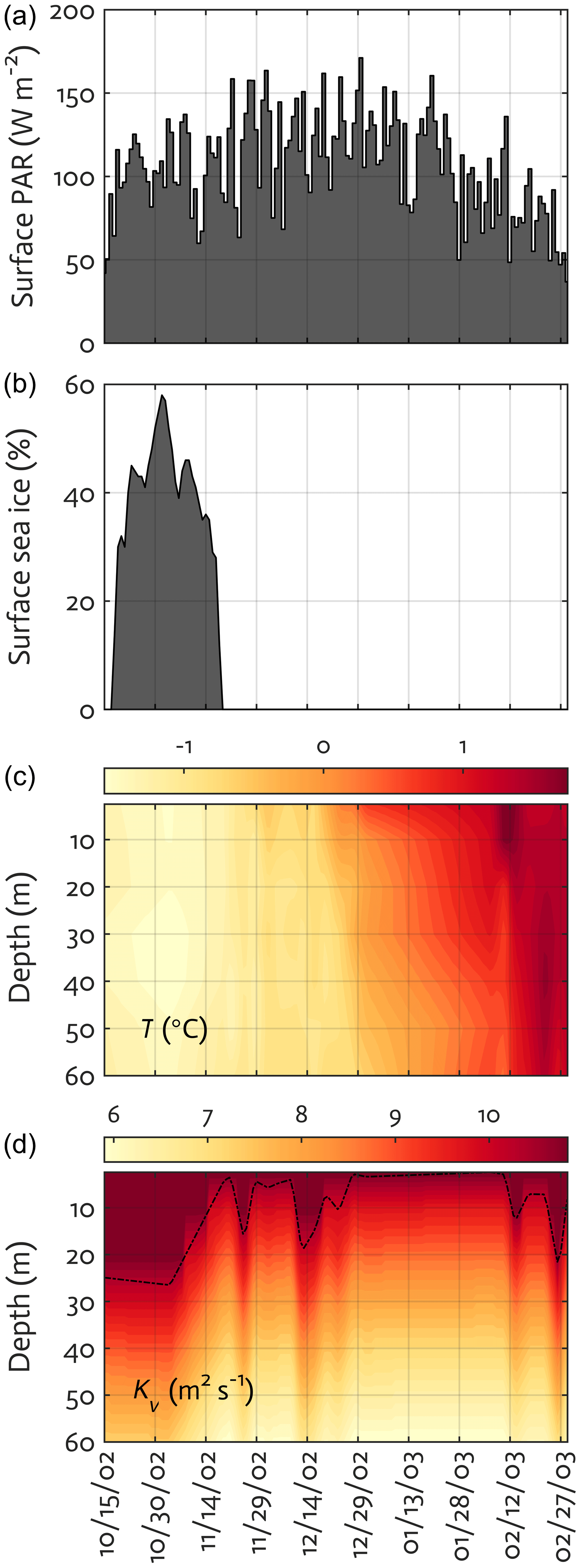
Figure 3Physical forcing used in the WAP-1D-VAR v1.0 model, including surface photosynthetically active radiation (PAR) (a), sea-ice concentration (b), water temperature (c), and vertical eddy diffusivity (d) overlaid with mixed layer depth (MLD; dashed line) in the modeled growth season of 2002–2003.
Given the routine observations of Palmer LTER available over the growth season (October–March), we simulate one example growth season with the most complete data coverage, from October 2002 to March 2003 (2002–2003 growth season hereafter), instead of a series of different growth seasons in a continuous manner. The example growth season simulations utilize this year's specific observed physical forcing fields and assimilated biological and biogeochemical observations. Each Palmer LTER growth season should be modeled to have its own unique optimized parameter set, as well as initial conditions and physical forcing that together determine the model solution for that year; however, only the 2002–2003 growth season simulations are modeled in this study for model analysis and evaluation.
3.2 Initial and boundary conditions
Model initial conditions are prescribed 135 d before the model start date for the growth season (15 October 2002) on 1 June 2002. This 135 d spinup is conducted to minimize the impact of initial conditions on the model output over the growth season. Initial conditions are prepared by optimizing the full growth seasonal cycle forced by climatological physics and assimilated with climatological observations and with the same bottom boundary conditions used in the optimization of the 2002–2003 growth season (i.e., climatological model; using climatological physics and observations averaged over nine growth-season periods between 2002–2003 and 2011–2012 except the 2007–2008 growth season due to its missing data). For the first climatological model simulation, initial conditions are prepared by adjusting manually following literature values (e.g., Luo et al., 2010). Due to strong interannual variability in the phytoplankton bloom phenology at Palmer Station, averaging across all these 9 years does not reflect distinct seasonal phytoplankton peaks, leading to underestimated phytoplankton values (not shown). To capture this non-linear aspect of the coastal WAP system, we construct the climatological year by applying a single time shift to all variables so that a seasonal PP peak of each year lines up with an average date of seasonal PP peaks from all years. Most biological initial conditions on 1 June are close to zero given the lack of active physiological processes in the very low light and the presence of sea ice during wintertime before the model growth season starts. All the data types are set to zero at the lower boundary (bottom) except for NO3, PO4, SDOC, SDON, and SDOP in which the climatological values at 65 m are used for lower boundary values (25.9, 1.9, 6.5, 0.6, and 0.03 mmol m−3, respectively).
3.3 Assimilated data
We include the data types directly related to corresponding model outputs, including a mix of ecosystem stocks or state variables – NO3, PO4, Chl for diatoms and cryptophytes, bacterial biomass, microzooplankton biomass, SDOC, POC, and particulate organic nitrogen (PON), as well as carbon flows among model stocks – bulk net PP and bacterial production (BP). These data sets have been sampled semi-weekly at Palmer Station E (64.77∘ S, 64.05∘ W), the same location where our model is set up, and are available from the Palmer LTER data website (see data availability). The distinction between diatoms and cryptophytes is established by assimilating phytoplankton taxonomic-specific Chl data for diatoms and non-diatom species derived from a high-performance liquid chromatography (HPLC) and CHEMTAX analysis (Schofield et al., 2017), but given cryptophytes being the second dominant species in the water samples at the study site, cryptophytes are assumed to represent all non-diatom species for modeling purposes. Given that POC (PON) from bottle filtration may capture both living biomass and detrital material, we adjust the observed POC (PON) by subtracting phytoplankton and bacterial C (N) biomass to estimate the detrital pool, in order to only include non-living particles to detrital pool. When phytoplankton or bacterial biomass data are not available, we assign climatological (2002–2003 to 2011–2012) fractions of POC (PON) to detrital pool. Phytoplankton and bacterial biomass accounts for 26 % of total POC and 29 % of total PON. In converting Chl to phytoplankton carbon (nitrogen) biomass, the maximum ChlC (ChlN) ratio submitted for optimization is used along with other reference ratios (Table 1). Microzooplankton biomass data are not available for the full time series, so their data from grazing experiments at Palmer Station (Garzio et al., 2013) are assimilated to at least provide constraints on bacterial and cryptophyte grazing processes. However, due to the discrepancy in the timing and location from model simulations of this study, the microzooplankton model–observation misfits are not analyzed in the present study. Krill biomass data are not assimilated due to the strong patchiness of their distribution that may hinder proper model optimization. The vertical profiles of most of the data types are assimilated, whereas average NO3 and PO4 concentrations in the mixed layer are assimilated due to the difficulty of simulating depth-dependent nutrient concentrations and the fact that net PP is mostly determined by surface nutrient concentrations (Luo et al., 2010). BP () is derived from the 3H-leucine incorporation rate () data using the conversion factor of 1.5 kg C (mol leucine)−1 incorporated (Ducklow, 2000). Bacterial biomass (mmol C m−3) is estimated from bacterial abundance measured by flow cytometry with the conversion factor of 10 fg C cell−1 (Fukuda et al., 1998). SDOC is calculated by subtracting the background concentration (41.2 mmol m−3 for the modeling site) from total DOC concentration.
3.4 Uncertainty analysis
Uncertainties of the optimized parameters are computed from a finite difference approximation of the complete Hessian matrix (i.e., second derivatives of the cost function with respect to the model parameters) during the iterative optimization process (details in Sect. 2.4). We then conduct Monte Carlo experiments to calculate the impact of the optimized parameter uncertainties on the model results. We first create an ensemble of parameter sets (n=1000) by randomly sampling values within the uncertainty ranges of the constrained parameters and then perform a model simulation using each parameter set. A total of 1000 Monte Carlo experiments were shown to be adequate from a series of tests with different numbers of Monte Carlo sampling (n=500–2000), where standard deviations of model-simulated values converged after >1000 Monte Carlo sampling (not shown). All uncertainty estimates are calculated following standard error propagation rules and presented as ±1 standard deviation in the study.
4.1 Model skill assessment
In the case of the example growth season (2002–2003) modeled in this study, the iterative data assimilation–parameter optimization procedure reduced by 58 % the misfits between observations and model output compared to the misfits obtained from the initial parameter values (Table 2). The optimized model solution satisfied the preset convergence criteria, with the low gradients of the total cost with respect to the optimized parameters and positive eigenvalues of the Hessian matrix. Notably, this was achieved by optimizing a subset of 12 (9 constrained and 3 optimized) parameters among the total of 72 optimizable parameters (Table 1, Sect. 4.2). To examine the sensitivity of the optimized model solution to the initial parameter choice, a series of new optimization experiments (n=15) was conducted with a varying subset of the initial parameter values perturbed by ±50 % of those used in the original optimization experiment (Table B1). These experiments showed that the optimized model results (i.e., the reference case; Table 1) were not sensitive to the initial choice of the parameters. The 15 different initial parameter sets resulted in a range of initial model–observation misfits, some substantially larger than the reference case (14.25–28.24 vs. 14.85 for the reference case). However, the total normalized optimized cost values of the 15 sensitivity experiments (5.79–7.19) were similar to that of the reference case of 6.42. In sensitivity experiment no. 12, the initial model–observation misfit was ∼2 times larger than that of the reference case, and there was up to 76 % of the reduction in the model–observational misfit (vs. 58 % of the reduction in the reference case; Table B1, Table 1). These results suggest that no matter where in parameter space the optimization process starts from, the optimization scheme takes the model cost function to similar local minima. Importantly, this was achieved by similar subsets of the optimized parameters: μDA, μCR, , and μMZ were optimized in all cases, while αDA, αCR, Θ, μBAC, gCR, , gBAC, μKR, gMZ, and remvKR were optimized except for a few cases (Table B1). The uncertainties of the optimized parameters were also similar among different optimizations, with most of the relative errors <0.5. Constrained parameter values and their uncertainty ranges averaged over the sensitivity experiments (Table B2) were comparable to those in the original optimization experiments (Table 1).
Table 2The observed mean (), coefficient of variation (CV), and target error (σ) of each assimilated data type used for calculating the cost function before and after optimization. J0 is the normalized cost function before optimization and Jf is the normalized cost function after optimization (Eq. 6). Data type units: mmol m−3 for NO3, PO4, bacterial biomass, SDOC, and POC; mg m−3 for diatom Chl, cryptophyte Chl, mmol N m−3 for PON; and for PP and BP. The average error (εbias) of each data type (for non-transformed or raw Chl and PP) is calculated from Stow et al. (2009) before and after optimization where a positive value indicates the model overestimation of the observation, and vice versa.
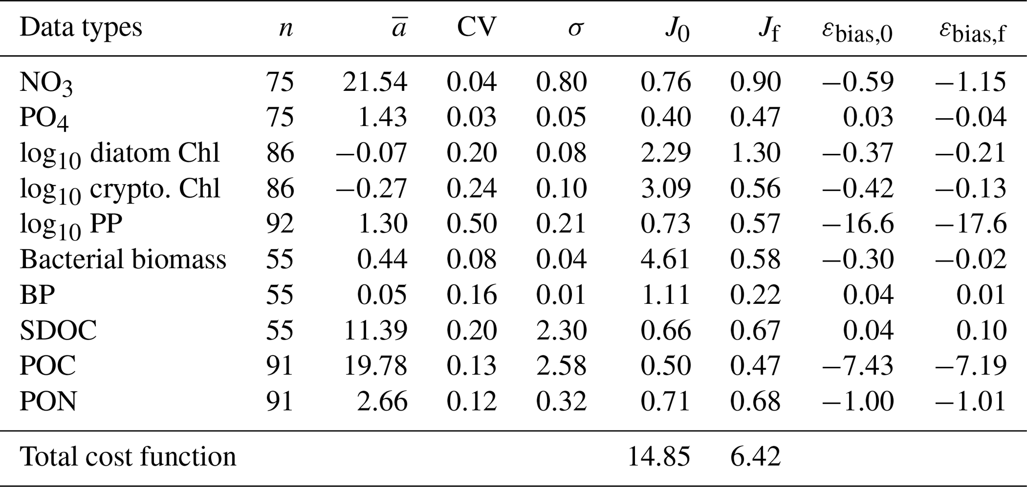
Overall, there was a good model–data fit with the largely decreased cost value for each data type after optimization (Table 2). Optimization yielded Jf close to 1 for all data types, compared to the initial model solution where three data types – diatom Chl, crypto Chl, and bacterial biomass – had particularly poor model fits to observations and underestimated error variances (J≫1). Compared to the initial (unoptimized) model results, the average errors (εbias, Doney et al., 2009; Stow et al., 2009) in the optimized model results indicated that diatom Chl, cryptophyte Chl, bacterial biomass, BP, and POC had reduced model biases, while NO3, PO4, PP, SDOC, and PON had increased model biases (for both positive and negative biases, defined as εbias>0 and εbias<0, for model overestimation and underestimation of the observation, respectively). Optimization resulted in the negative model bias for PO4, compared to the positive model bias in the initial model results. The point-to-point comparison plots showed that there were seasonally consistent, negative model biases for PP, POC, and PON (Fig. B1). Model skill was further evaluated with a Taylor diagram (Taylor, 2001) summarizing the statistics of the correlation coefficient between model output and observations, normalized standard deviation (by the standard deviation of the observations), and centered (bias removed) root-mean-square difference (RMSD) for each data type, in which a better model skill is characterized by a higher correlation, a normalized standard deviation close to 1, and a lower RMSD (Fig. 4). Optimization resulted in better model skills for cryptophyte Chl, PP, BP, and bacterial biomass via increased correlation coefficients and lowered RMSD (Fig. 4b), compared to those in the unoptimized model results (Fig. 4a). After optimization, the normalized standard deviations of PP, BP, bacterial biomass, phosphate, POC, and PON were closer to 1 (Fig. 4b). Direct comparisons with the observational data showed that the optimized model parameter set captured better the increases in diatom biomass early in the season, cryptophyte biomass in January, and bacterial biomass in mid-February, compared to the unoptimized model parameter set (Figs. 5a and b and B2).
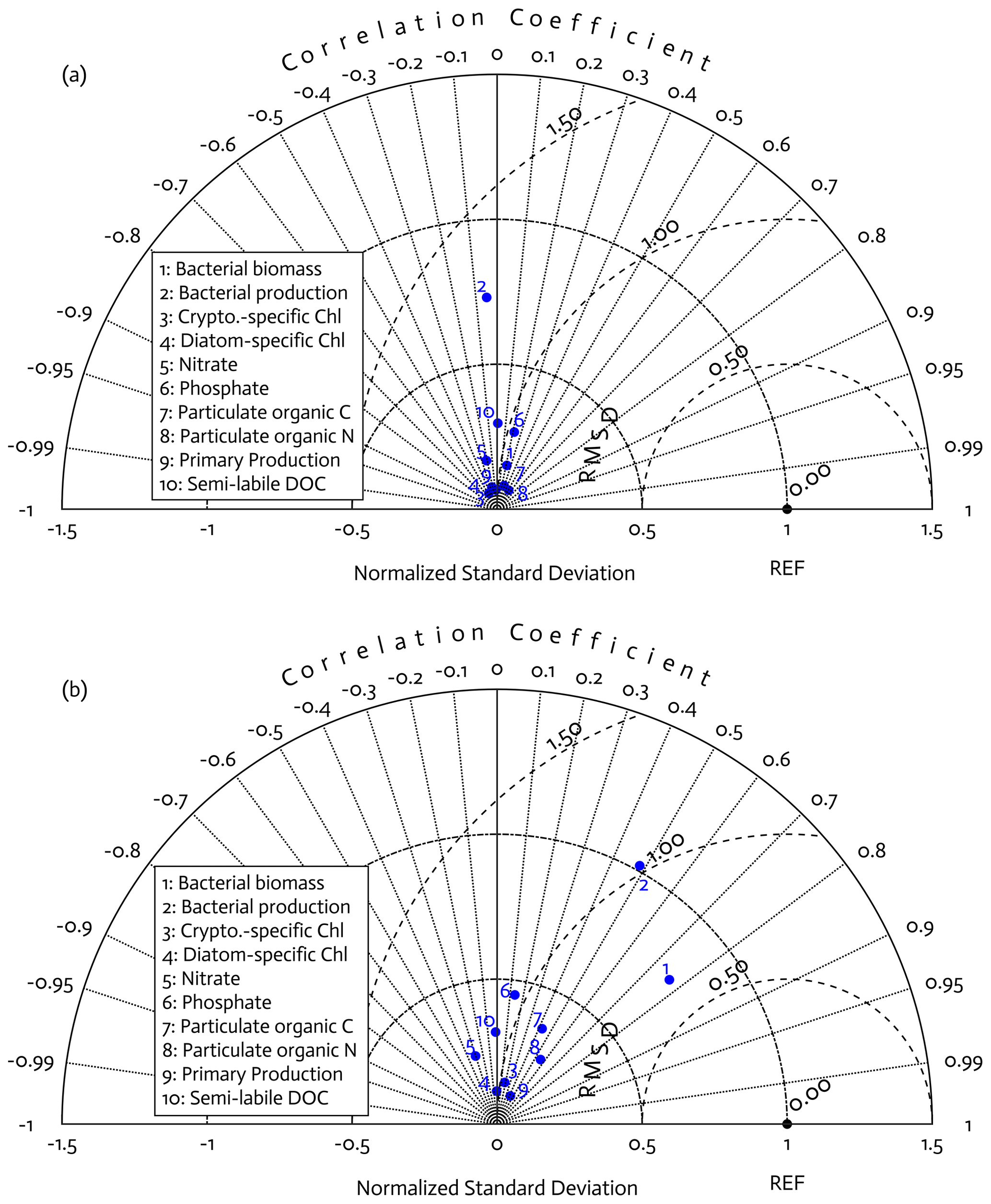
Figure 4Model skill assessment: the Taylor diagrams using a polar-coordinate system summarizing the model–observation correspondence for each model stock and flow for the modeled growth season of 2002–2003 before (a) and after optimization (b). The angular coordinate for the Pearson correlation coefficient (r), the distance from the origin for the standard deviation normalized by the standard deviation of the observation, and the distance from point (1,0), marked as REF on x axis, for the centered (bias removed) root-mean-square difference (RMSD) between model results and observations.
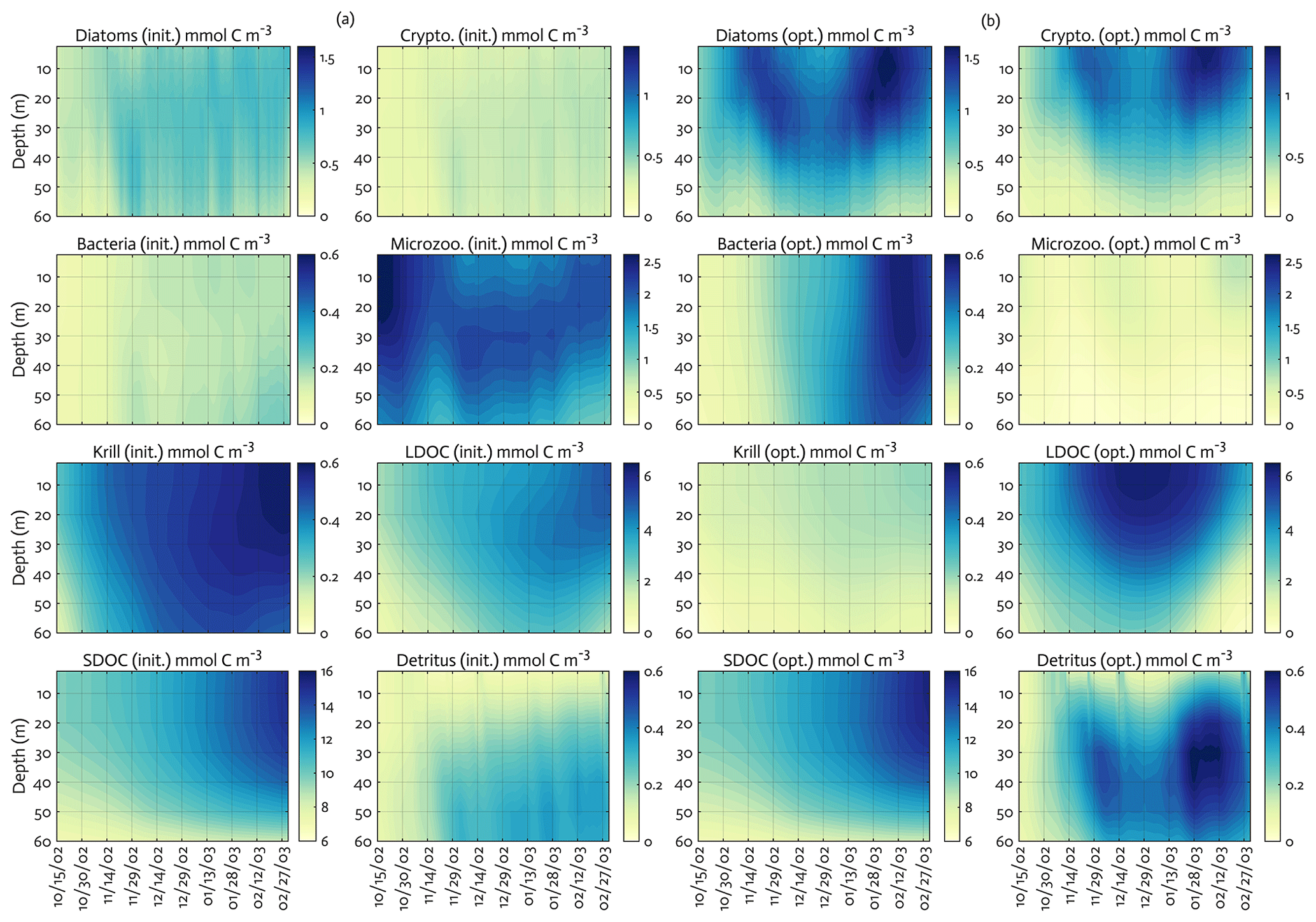
Figure 5The model state variables for the modeled growth season of 2002–2003 (x axis; month/day) for before (a) and after optimization (b) with init. as the initial (unoptimized) model results and opt. as the optimized model results. The error (standard deviation) of each model state variable from the Monte Carlo experiments (n=1000) is available in Fig. B3.
4.2 Optimized parameters
The number of the optimized parameters in this study is small and comparable to those from other data-assimilative models focused on different marine environments (Friedrichs, 2001; Friedrichs et al., 2006, 2007; Luo et al., 2010). This is consistent with the general behavior of marine plankton ecosystem models, in which well-posed model solutions would be found with only a subset of independent model parameters due to many cross-correlated parameters inherent in non-linear model equations (Fennel et al., 2001; Harmon and Challenor, 1997; Matear, 1996; Prunet et al., 1996a, b). Ecosystem models with a relatively large number of unconstrained parameters (i.e., equivalent to the optimized parameters with high uncertainties in the present study) might reduce total costs to a greater extent but could possess low predictive skill as a result of being overtuned to fit noise in the observations (Friedrichs et al., 2007). Also, there are several field- and lab-based studies at the study site or in a similar polar environment that reported the values of the model parameters used in the WAP-1D-VAR v1.0 model, including the bacterial growth rate of 0.82 d−1, total phytoplankton (including large cells like diatoms) growth rate of 0.33–0.55 d−1, nanophytoplankton (corresponding to cryptophytes) growth rate of 0.52–0.99 d−1 (Garzio et al., 2013), and the microzooplankton growth rate of up to 1.0 d−1 (Caron et al., 2000). The optimized values of the maximum bacterial, diatom, cryptophyte, and microzooplankton growth rates in this study were 1.06 d−1 (0.93–1.20 d−1), 0.77 d−1 (0.68–0.88 d−1), 0.72 d−1 (0.61–0.85 d−1), and 1.18 d−1 (1.10-1.26 d−1), falling in the ranges of those measured bacterial, total phytoplankton, nanophytoplankton, and microzooplankton growth rates, respectively.
The ensemble of the model state variables and flows obtained from the Monte Carlo experiments had generally small standard variations at each model time step and grid, suggesting the robustness of the modeled fields against the variations in the optimized parameter values (Figs. B3 and B4). To examine the translation of the optimized parameter values to altered functioning of the WAP biogeochemical processes, we compared two different sets of the model simulation results – one based on the initial parameter values (Figs. 5a, 6a, and 7a) and the other based on the optimized parameter values (Figs. 5b, 6b, and 7b). However, due to the non-linearities in the model, it is not straightforward to identify what causes the parameter variations, except for a few cases in which the changes in the parameter values are clearly linked to the difference in the model state variables and flows. The first case is the relation of the increased gBAC value (bacterial half-saturation concentration in microzooplankton grazing, mmol C m−3) to the elevated bacterial accumulations after optimization (Table 1, Figs. 5 and 7). The second case is the link between Θ (maximum ChlN ratio, g Chl a (mol N)−1) and the relative dominance of cryptophytes in total phytoplankton accumulations. It has been demonstrated that the variations of Θ are driven by an imbalance between the rate of light absorption and energy demands for photosynthesis and biosynthesis in phytoplankton cells (Geider et al., 1997). Θ can also change because of the variations in phytoplankton photo-acclimation or physiological differences across phytoplankton groups, from a lower Θ value for smaller species to a higher Θ value for larger diatom cells (Geider, 1987). Θ was optimized to a 30 % lower value than the initial parameter value (Table 1), in order to simulate the relatively larger proportion of cryptophytes in total phytoplankton accumulations in the optimized model results compared to the unoptimized model results (Figs. 5 and 7). By contrast, the remaining cases are not as clear because the first-order impact of parameter variations on the model results is less direct and more nuanced. Compared to the unoptimized results, the decreases in μDA (diatom C-specific maximum growth rate, d−1), μCR (cryptophytes C-specific maximum growth rate, d−1), αDA (initial slope of P–I curve of diatoms, ), and αCR (initial slope of P–I curve of cryptophytes, ) did not lead to decreased diatom and cryptophyte accumulations, presumably due to decreased gMZ (microzooplankton half-saturation concentration in krill grazing, mmol C m−3) and increased remvKR (krill removal rate by higher trophic levels, ) after optimization (Table 1, Figs. 5 and 7). Similarly, the decreased μBAC (maximum bacterial growth rate, d−1) and the increased (bacterial maximum active respiration rate, d−1) did not lead to decreased bacterial accumulations, presumably due to the increased gBAC (bacterial half-saturation concentration in microzooplankton grazing, mmol C m−3) and the decreased gMZ (microzooplankton half-saturation concentration in krill grazing, mmol C m−3).
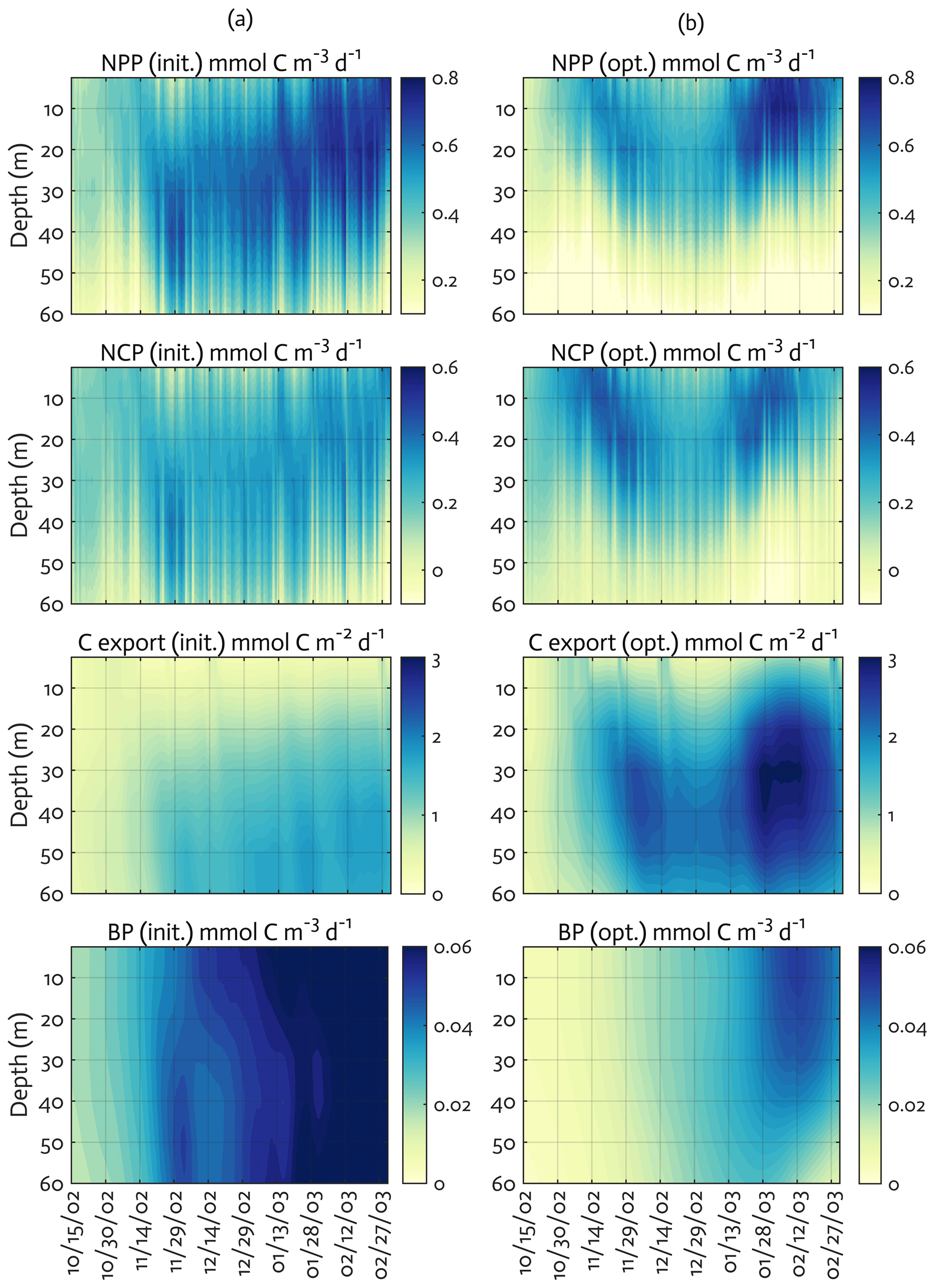
Figure 6Model ecosystem indices before (a) and after optimization (b). The key ecosystem indices for the modeled growth season of 2002–2003 (x axis; month/day), with init. as the initial (unoptimized) model results and opt. as the optimized model results. NPP: net primary production, NCP: net community production, C export flux: particulate organic carbon (POC) export flux, and BP: bacterial production. The error (standard deviation) of each rate process from the Monte Carlo experiments (n=1000) is available in Fig. B4.
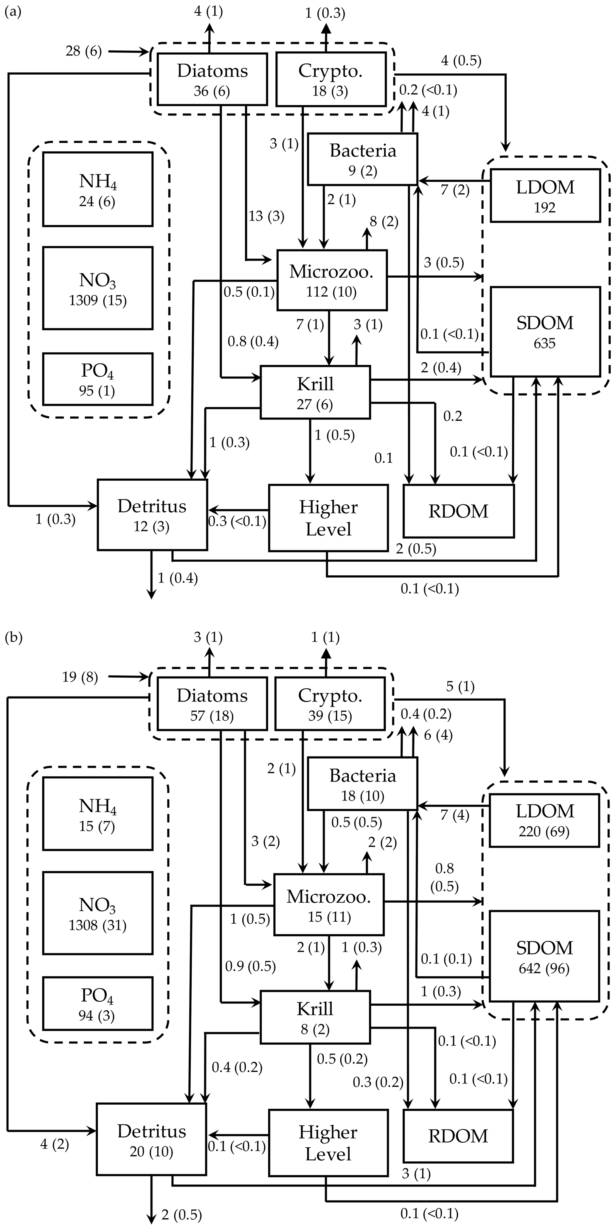
Figure 7Depth-integrated (0–60 m) carbon stocks (mmol C m−3), flows (), and POC export flux at 60 m () averaged over the modeled austral growth season (October 2002–March 2003) before (a) and after optimization (b). Values in parentheses as uncertainties from season averaging (a) and as uncertainties propagated from season averaging and depth integration of the Monte Carlo errors for panel (b).
4.3 Ecosystem indices
We calculated key ecosystem indices for the modeled growth season, including NPP (directly comparable to 14C–PP observations), net community production (NCP; i.e., NCP=NPP – bacterial, microzooplankton, and krill respiration), BP, and POC export (sinking) flux (Fig. 6). Setting an upper limit for lateral or vertical carbon export from the euphotic zone (Dugdale and Goering, 1967), over appropriate timescales and space scales, NCP is quantitatively equivalent to new production that is supported via external sources of nitrogen (Ducklow and Doney, 2013). In both optimized and unoptimized model results, NPP increased after complete sea-ice retreat, but a brief ice-edge bloom was simulated under sea ice at the beginning of the growth season (Figs. 3 and 6). Seasonal patterns of NCP resembled those of NPP and occasionally fell below zero (i.e., the net heterotrophy) in subsurface waters for both optimized and unoptimized cases (Fig. 6). The POC export flux increased over time and reached the maximum value at the end of the growth season in both model results, but there were two major POC flux events separated by weaker, in-between flux events in December in the optimized results that the initial model results did not capture (Fig. 6b). After optimization, the correlation coefficients adjusted from 0.88 to 0.36, 0.89 to 0.68, and 0.45 to 0.73 for the NPP vs. NCP pair, the NPP vs. BP pair, and the NCP vs. POC export flux (lagged by 30 d) pair (all p<0.001). In the optimized model results, the growth-season mean of the depth-integrated NPP, NCP, and BP in the 60 m water column, and the 30 d lagged POC export flux at 60 m were 19±8 , 10±3 , 1±1 , and 2±0.3 (uncertainties propagated from season averaging in Fig. 6b and Monte Carlo uncertainties in Fig. B4), compared to 28±6 , 13±3 , 3±1 , and 2±0.2 in the unoptimized model results (uncertainties from season averaging in Fig. 6a).
The mean e ratio, defined as the growth-season mean of the 30 d lagged POC export flux divided by the growth-season mean NPP, was 0.11±0.05 (uncertainties propagated from season averaging in Fig. 6b and Monte Carlo uncertainties in Fig. B4) in the optimized model results, compared to 0.07±0.02 (uncertainties from season averaging in Fig. 6a) in the unoptimized model results. The mean f ratio, defined as the amount of NO3 uptake divided by the amount of NO3 and NH4 uptake both, was 0.88±1.52 in the optimized model results, compared to 0.84±0.19 in the unoptimized model results (not shown). The higher mean f ratio relative to the mean e ratio in this study implies an imbalance between production and export at the study site, at least during the modeled period. Excess new production relative to export production (as derived from sediment traps and 234Th disequilibrium; Ducklow et al., 2018) was previously observed in the WAP, presumably due to diel vertical migration, DOM export, lateral export, and diffusive loss of PON via diapycnal mixing (Stukel et al., 2015). Stukel et al. (2015) reported up to 5 times larger new production via NO3 uptake than export production via Th-based N export along the coastal WAP. Several additional mechanisms might be responsible for driving the discrepancy between production and export. First, given that the assimilated pool of suspended POC in the model formulation is not a good indicator of a rapidly sinking detrital pool dominating particle export, the WAP-1D-VAR v1.0 model does not capture large, short-lived particle flux events (e.g., fecal pellets produced by a large swarm of krill), underestimating POC export flux. Second, the WAP-1D-VAR v1.0 model export scheme does not consider DOC export that would lower the production–export discrepancy. Finally, RDOC is not explicitly modeled in the model, due to its much longer timescale than the model timescale, so accumulated and not-exportable RDOC pool would contribute to the deviation of the modeled e ratio from the modeled f ratio. Indeed, the modeled mean e ratios in our study, for both optimized and unoptimized cases, are situated at the lower end of the range of the e ratios measured or estimated in the WAP waters (Ducklow et al., 2018; Sailley et al., 2013; Stukel et al., 2015; Weston et al., 2013), but optimization increased the e ratio by 60 % and thus made it closer to the literature values.
The mean BPNPP ratio was 0.05±0.06 (uncertainties propagated from season averaging in Fig. 6b and Monte Carlo uncertainties in Fig. B4) in the optimized model results, compared to 0.11±0.04 (uncertainties from season averaging in Fig. 6a) in the unoptimized model results. The modeled mean BPNPP ratio for both optimized and unoptimized cases corresponds well to the estimates from other measurement- and observation-based studies (Ducklow et al., 2012; Kim and Ducklow, 2016). Relatively low bacterial activity in productive Antarctic waters, typically reflected as a low BPPP ratio, has been attributed to low LDOM availability for bacterial growth (Kirchman et al., 2009), low temperature (Pomeroy and Wiebe, 2001), or top-down control via grazing and viral lysis (Bird and Karl, 1999).
4.4 Mean carbon stocks and flows
We summarized the growth-season means of the carbon stocks and flows in the entire food web (Fig. 7). The WAP-1D-VAR v1.0 model captured several key WAP ecological and biogeochemical features, including the lack of macronutrient limitation (NO3 and PO4 drawdown by phytoplankton utilization but remaining well above their half-saturation constants, Table 1) and comparable values of the assimilated and non-assimilated model state variables (Ducklow et al., 2007, 2012, 2018; Kim et al., 2016; Moline et al., 2008; Smith et al., 2008), providing confidence in the model simulations. For instance, growth-season measurements in 2017–2018 at Palmer Station showed a strongly patchy krill distribution, with the mean biomass of 0.12±0.04 mmol C m−3 and the maximum biomass of 0.57 mmol C m−3 when krill were present (unpublished data provided by D. Steinberg), falling in the range of the modeled krill biomass values (0.13±0.03 mmol C m−3; calculated from Fig. 7b). The WAP-1D-VAR v1.0 model also simulated several important ecosystem metrics comparable to other statistical modeling studies. For instance, the modeled phytoplankton seasonal patterns in the present study are consistent with physicochemical attributes revealed by a distinct ecological seascape pattern in the coastal WAP (Bowman et al., 2018), including low Chl and high nutrients in the first half of the growth season followed by high Chl and low nutrients in the second half of the growth season. A steady-state-solution-based inverse modeling study quantified different food-web states using ecosystem network indices from Palmer LTER annual summer cruises along the WAP shelf region (Sailley et al., 2013). Their network indices include the ratio of C export to total PP (i.e., equivalent to e ratio in our study) and the ratio of recycling (the sum of flows into respiration and DOC pool) to total PP, where more (less) recycling favorable microbial food webs are characterized by greater (smaller) ratios of recycling to total PP and smaller (greater) ratios of total C export to total PP (Legendre and Rassoulzadegan, 1996). As discussed above, the modeled mean e ratio in the present study is smaller than the estimates in the inverse modeling study for the WAP shelf region (Sailley et al., 2013) but consistent with their conclusion on the food-web status of the modeled growth season (2002–2003) positioned on the microbial food-web side. The discrepancy in the e-ratio values between the present study and Sailley et al. (2013) may be attributed to fundamentally different model formulation (i.e., time-evolving modeling for the WAP-1D-VAR v1.0 model vs. steady-state modeling) and optimization approach, or due to relatively strong microbial food-web activity at our coastal site compared to the shelf region. Microbial food-web activity can be approximated by quantifying the amount of fixed carbon flowing through heterotrophic bacteria (Carlson et al., 1999; del Giorgio and Cole, 1998; Ducklow, 2000; Ducklow et al., 2012). According to this approach, microbial food-web activity from the optimized model results was around 38 %±16 %, calculated as the ratio of bacterial L- and SDOC uptake to PP (i.e., (arrow 13 + arrow 14)arrow 1 in Fig. 1, mean ± uncertainties from season averaging and Monte Carlo uncertainties in Fig. 7b). On average, SDOC supported 1 %±2 % of the total bacterial C uptake or C demand (i.e., arrow 14/(arrow 13 + arrow 14) in Fig. 1, mean ± uncertainties from season averaging and Monte Carlo uncertainties in Fig. 7b) but could be an important bacterial C source when LDOC became scarce as the growth season progressed (Fig. 5b). Indeed, several observational studies speculated that the WAP bacteria utilize SDOM in short of LDOM (Ducklow et al., 2011; Kim and Ducklow, 2016; Luria et al., 2017).
We developed the WAP-1D-VAR v1.0 model, a one-dimensional variational data assimilation model specific to the coastal WAP region, evaluated the model performance and robustness using a variety of quantitative metrics, and discussed the model applicability with regard to capturing the key WAP ecological and biogeochemical features using the data from the example growth season. The data assimilation scheme significantly reduced the model–observation misfits via the optimized model parameter set that adjusted the simulation to better match the Palmer LTER observations in 2002–2003. We also explored the nuanced question of how the observations influenced the data assimilation process, drove the variations in optimized parameter values relative to their corresponding initial parameter values, and affected the resulting model simulations. The WAP-1D-VAR v1.0 model successfully simulated the variables and flows not included in data assimilation, with the values consistent and comparable with other measurement- and observation-based studies in the coastal WAP. Importantly, the data assimilation scheme enabled the available observational data to constrain processes that were poorly understood, including the partitioning of NPP by different phytoplankton groups, the optimal ChlC ratio of the WAP phytoplankton community, and the partitioning of DOC pools with different lability. Up to this point, a range of observational studies has provided snapshots of ecosystem and biogeochemical processes in the WAP. Yet, we have little understanding of the driving processes that underlie the connections between each component in complex food-web interactions. We used data-assimilative modeling to glue these snapshots together to better explain the observed dynamics and further understand the previously poorly constrained processes in the coastal WAP system.
A1 Temperature effect
A2 Diatom processes
-
Cellular quota (ratio):
-
N and P limitation function:
-
Maximum primary production rate:
-
C-specific gross primary production:
-
Limitation on N and P uptake:
-
N assimilation:
-
P assimilation:
-
Chlorophyll production:
-
Respiration:
-
Passive excretion of LDOM:
-
Active excretion of LDOC:
-
Active excretion of SDOC:
-
Active excretion of SDON and SDOP (if , otherwise 0):
-
Partitioning between LDOM and SDOM:
-
POM production by aggregation:
-
Grazing by microzooplankton:
-
Grazing by krill:
-
The net growth rate equations:
A3 Cryptophyte processes
-
Cellular quota (ratio):
-
N and P limitation function:
-
Maximum primary production rate:
-
C-specific gross primary production:
-
Limitation on N and P uptake:
-
Nitrogen assimilation:
-
Phosphorus assimilation:
-
Chlorophyll production:
-
Respiration:
-
Passive excretion of LDOM:
-
Active excretion of LDOC:
-
Active excretion of SDOC:
-
Active excretion of SDON and SDOP (if , otherwise 0):
-
Partitioning between LDOM and SDOM:
-
POM production by aggregation:
-
Grazing by microzooplankton:
-
The net growth rate equations:
A4 Bacterial processes
-
Cellular quota (ratio):
-
N and P limitation function:
-
Maximum available LDOC and SDOC:
-
Bacterial uptake of LDOC and SDOC (i.e., bacterial gross C growth):
-
Bacterial N uptake:
if Nf,BAC<1,
else,
-
Bacterial P uptake:
-
Respiration:
-
RDOC release:
-
Remineralization of inorganic nutrients:
if and (i.e., C in short)elseif and (i.e., N in short)
else (i.e., P in short)
-
SDOM excretion to adjust stoichiometry:
if and (i.e., C in short)else if and (i.e., N in short)
else (i.e., P in short)
-
Grazing by microzooplankton:
-
Viral mortality:
-
Net flux of inorganic nutrients through bacteria:
-
The net growth rate equations:
A5 Microzooplankton processes
-
Cellular quota (ratio):
-
Gross growth:
-
LDOM excretion:
-
SDOM excretion:
-
SDOM excretion to adjust stoichiometry:
-
Remineralization of inorganic nutrients:
-
Respiration:
-
POM production:
-
Grazing by krill:
-
The net growth rate equations:
A6 Krill processes
-
Cellular quota (ratio):
-
Gross growth:
-
LDOM excretion:
-
SDOM excretion:
-
SDOM excretion to adjust stoichiometry:
-
Remineralization of inorganic nutrients:
-
Respiration:
-
POM production:
-
RDOC release:
-
Removal by higher trophic levels
-
The net growth rate equations:
A7 Detrital processes
-
Dissolution:
-
The net change equations:
where
A8 DOM processes
-
Conversion of SDOM to RDOM:
-
The net change equations:
A9 Dissolved inorganic nutrient processes
-
Nitrification:
-
The net change equations:
where
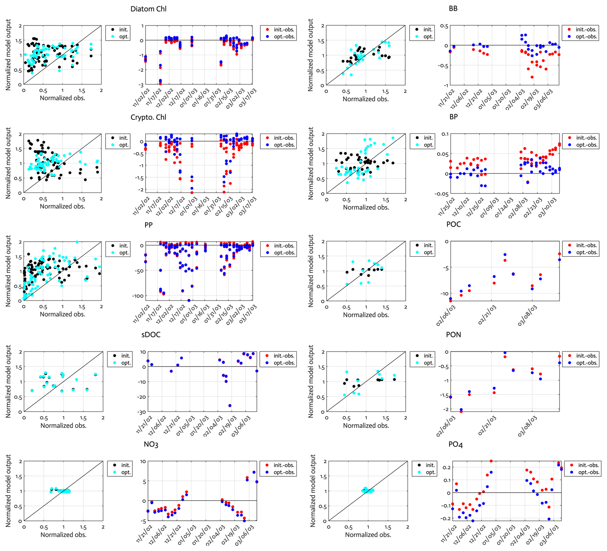
Figure B1Comparison of the observations to the initial (unoptimized) and optimized model results. The dot points in the second panels represent how much larger model output value is compared to the corresponding observational data (i.e., the model value minus the observational value). Normalized observation: observations normalized by the mean of each model state variable.
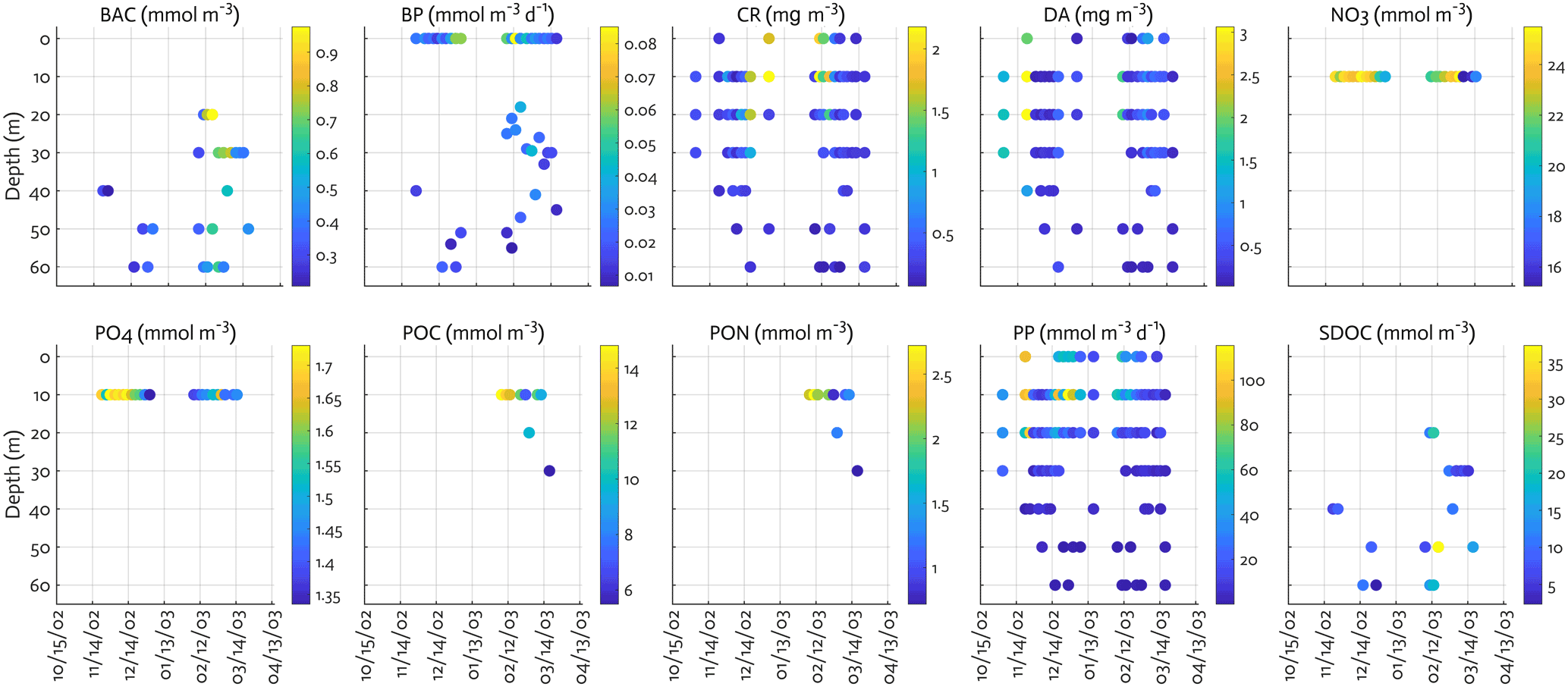
Figure B2Observations assimilated for each data type. BAC: bacterial biomass, CR: cryptophyte Chl, DA: diatom Chl.
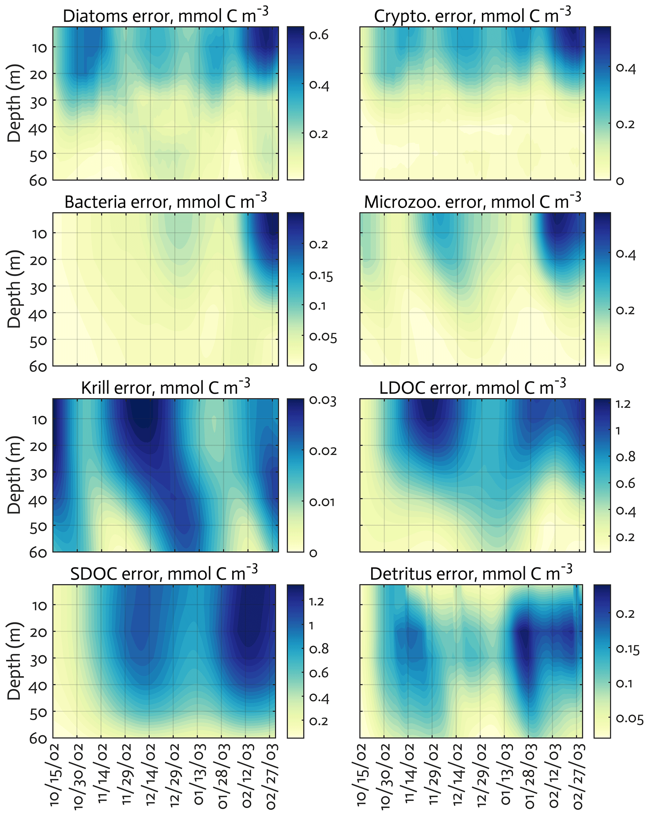
Figure B3The uncertainties (standard deviation) of the model state variables for the modeled growth season of 2002–2003 (x axis; month/day) from the Monte Carlo experiments (n=1000). Note the different contour scales among panels.

Figure B4The uncertainties (standard deviation) of the ecosystem indices for the modeled growth season of 2002–2003 (x axis; month/day) from the Monte Carlo experiments (n=1000). Note the different contour scales among panels.
Table B1Sensitivity tests to varying initial parameter values. The parameters with “n/a” in the parentheses are optimized parameters with large relative uncertainties (i.e., “optimized parameters”). The 50 % perturbations to AE, wnsv, and remin (Table 1) are considered ecologically unrealistic and therefore excluded from these sensitivity experiments.
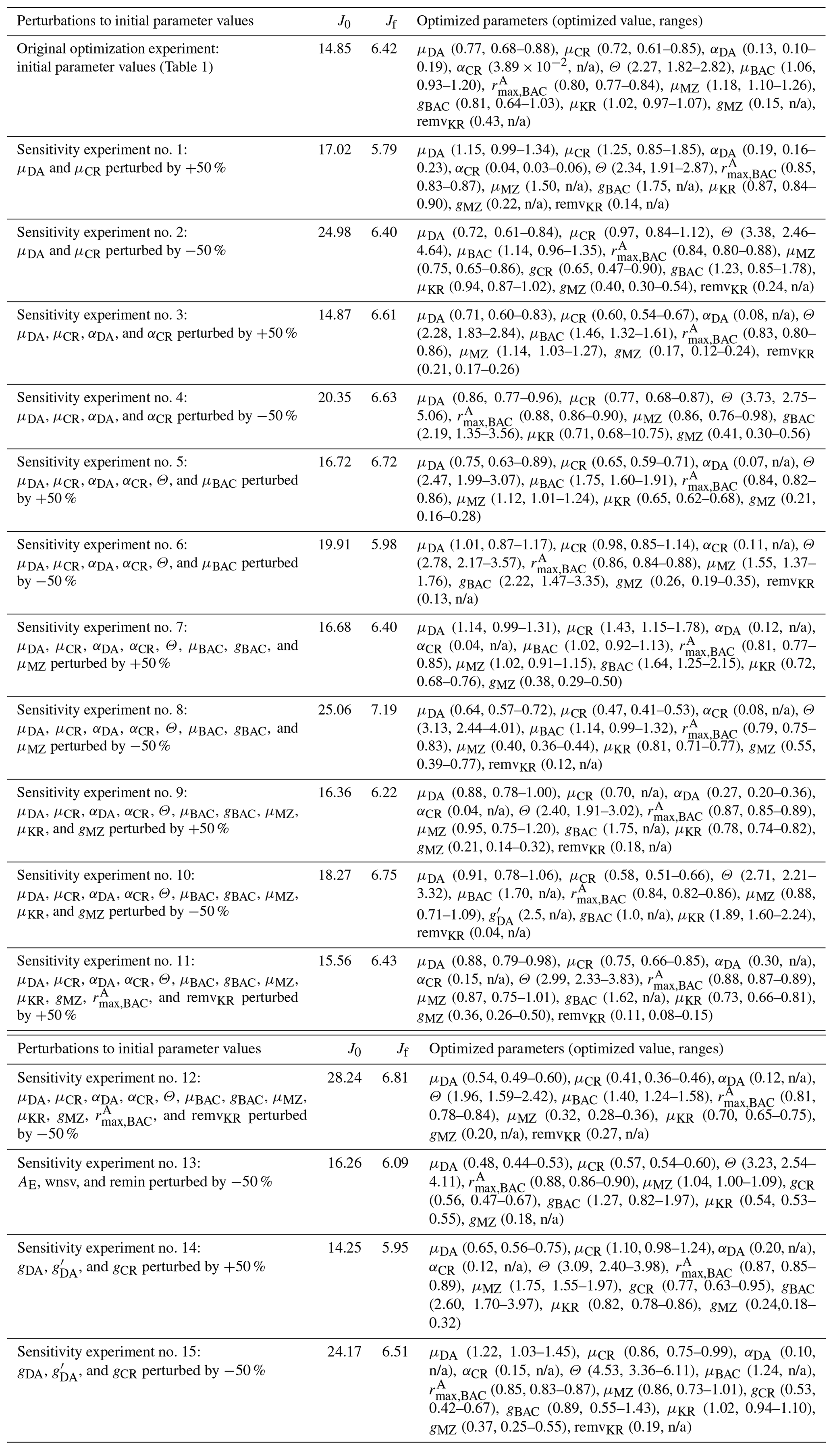
Table B2Summary of model parameters from initial parameter perturbation experiments. Summary of the model parameter symbol and definition, initial parameter values (p0,ref) and optimized values (pf,ref) for the original (reference) experiments (Table 1), and initial parameter values (p0) and optimized values (pf) averaged from the sensitivity experiments (n=15). p0,ref and the mean p0 are the same for most parameters because of the perturbations by ±50 % their original initial parameter values (with standard deviation in parentheses), while p0,ref and the mean p0 are different for AE and wnsv because of the perturbations only by −50 % their original initial parameter values (with standard deviation in parentheses). Numbers in parentheses for pf are the uncertainty ranges (lower and upper bounds) averaged across the sensitivity experiments as follows. First, for each sensitivity experiment, lower and upper bounds of the constrained parameter are calculated as and (where pf is the value of the constrained parameter and σf is the square roots of diagonal elements of the inverse of the Hessian matrix), respectively. Then we form the “lower (upper) bound parameter set” that only consists of the lower (higher) bounds of the constrained parameters from each experiment, and average those across the sensitivity experiments (n=15) to calculate the lower (upper) bound listed in parentheses.
The Tangent linear and Adjoint Model Compiler (TAPENADE) used to construct an adjoint model is available online (https://team.inria.fr/ecuador/en/tapenade/, Inria at Sophia Antipolis, 2021). The current version of the WAP-1D-VAR model (v1.0) is available from the project website: https://zenodo.org/record/5041139 (Kim et al., 2021) under the Creative Commons Attribution 4.0 International license. The exact version of the model used to produce the results, input data, and scripts to run the model and produce the plots for all the simulations presented in this paper is archived on Zenodo (Kim et al., 2021) (26 January 2021). WAP-1D-VAR v1.0: A One-Dimensional Variational Data Assimilation Model for the West Antarctic Peninsula (version v1.0); https://doi.org/10.5281/zenodo.5041139; Kim et al., 2021). A user manual is available as a separate Supplement to this article.
Complete Palmer LTER time-series data used for data assimilation are available online (http://pal.lternet.edu/data, PAL-LTER, 2021). Surface downward solar radiation flux data used for physical forcing of the model simulations can be found at the National Centers for Environmental Prediction website (https://www.esrl.noaa.gov/psd/data/gridded/data.ncep.reanalysis.surface.html, NOAA-ESRL, 2021).
The supplement related to this article is available online at: https://doi.org/10.5194/gmd-14-4939-2021-supplement.
HHK developed the model, performed model simulations, and wrote the manuscript. YWL contributed to model simulations. HWD, OMS, and DKS provided observational data. SCD supervised the research and especially the manuscript.
The authors declare that they have no conflict of interest.
Publisher's note: Copernicus Publications remains neutral with regard to jurisdictional claims in published maps and institutional affiliations.
We thank the many Palmer LTER team members and Palmer Station support staff for collecting, measuring, and analyzing the field samples and for providing the data sets used in the present study. We also thank Le Xie for providing protocols for the parameter optimization and adjoint models, Cristina Schultz for providing the initial parameter values of the model parameters, Nicole Waite for compiling HPLC data, and Joe Cope and Lori Garzio for compiling the zooplankton data. Computing resources for model simulations were provided on the Rivanna high-performance computing system by the Advanced Research Computing Services of the University of Virginia and on the Poseidon high-performance computing system by Woods Hole Oceanographic Institution.
Hyewon Heather Kim and Scott C. Doney were supported by the National Aeronautics and Space Administration Ocean Biology and Biogeochemistry Program (grant no. NNX14AL86G) and the US National Science Foundation Office of Polar Programs (grant no. PLR-1440435 to Hugh W. Ducklow at Columbia University; Palmer LTER). Hyewon Heather Kim was additionally supported by the Investment in Science Fund and the Reuben F. and Elizabeth B. Richards Endowed Fund from Woods Hole Oceanographic Institution. Oscar M. Schofield and Deborah K. Steinberg were supported by US NSF grant no. PLR-1440435. Ya-Wei Luo was supported by National Natural Science Foundation of China project no. 41890802.
This paper was edited by Heiko Goelzer and reviewed by Jann Paul Mattern and one anonymous referee.
Armstrong, R. A.: Optimality-based modeling of nitrogen allocation and photo acclimation in photosynthesis, Deep-Sea Res. II, 53, 513–531, 2006.
Bertilsson, S., Berglund, O., Karl, D. M., and Chisholm, S. W.: Elemental composition of marine Prochlorococcus and Synechococcus: Implications for the ecological stoichiometry of the sea, Limnol. Oceanogr., 48, 1721–1731, https://doi.org/10.4319/lo.2003.48.5.1721, 2003.
Biddanda, B. and Benner, R.: Carbon, nitrogen and carbohydrate fluxes during the production of particulate and dissolved organic matter by marine phytoplankton, Limnol. Oceanogr., 42, 506–518, 1997.
Bird, D. F. and Karl, D. M.: Uncoupling of bacteria and phytoplankton during the austral spring bloom in Gerlache Strait, Antarctic Peninsula, Aquat. Microb. Ecol., 19, 13–27, https://doi.org/10.3354/ame019013, 1999.
Bjørnsen, P. K.: Phytoplankton exudation of organic matter: Why do healthy cells do it?, Limnol. Oceanogr., 33, 151–154, 1988.
Bowman, J. S. and Ducklow, H. W.: Microbial Communities Can Be Described by Metabolic Structure: A General Framework and Application to a Seasonally Variable, Depth-Stratified Microbial Community from the Coastal West Antarctic Peninsula, Plos One, 10, e0135868, https://doi.org/10.1371/journal.pone.0135868, 2015.
Bowman, J. S., Kavanaugh, M. T., Doney, S. C., and Ducklow, H. W.: Recurrent seascape units identify key ecological processes along the western Antarctic Peninsula, Glob. Change Biol., 24, 3065–3078, https://doi.org/10.1111/gcb.14161, 2018.
Campbell, J. W.: The lognormal distribution as a model for bio-optical variability in the sea, J. Geophys. Res.-Oceans, 100, 13237–13254, https://doi.org/10.1029/95JC00458, 1995.
Caron, D. A., Dennett, M. R., Lonsdale, D. J., Moran, D. M., and Shalapyonok, L.: Microzooplankton herbivory in the Ross sea, Antarctica, Deep-Sea Res. Pt. II, 47, 3249–3272, 2000.
Carlson, C. A., Bates, N. R., Ducklow, H. W., and Hansell, D. A.: Estimation of bacterial respiration and growth efficiency in the Ross Sea, Antarctica, Aquat. Microb. Ecol., 19, 229–244, 1999.
Carvalho, F., Kohut, J., Oliver, M. J., Sherrell, R. M., and Schofield, O.: Mixing and phytoplankton dynamics in a submarine canyon in the West Antarctic Peninsula, J. Geophys. Res., 121, 5069–5083, https://doi.org/10.1002/2016JC011650, 2016.
Clarke, A., Griffiths, H. J., Barnes, D. K. A., Meredith, M. P., and Grant, S. M.: Spatial variation in seabed temperatures in the Southern Ocean: Implications for benthic ecology and biogeography, J. Geophys. Res.-Biogeo., 114, G03003, https://doi.org/10.1029/2008JG000886, 2009.
Cook, A. J., Fox, A. J., Vaughan, D. G., and Ferrigno, J. G.: Retreating Glacier Fronts on the Antarctic Peninsula over the Past Half-Century, Science, 308, 541–544, https://doi.org/10.1126/science.1104235, 2005.
del Giorgio, P. A. and Cole, J. J.: Bacterial Growth Efficiency in Natural Aquatic Systems, Annu. Rev. Ecol. Syst., 29, 503–541, https://doi.org/10.1146/annurev.ecolsys.29.1.503, 1998.
Doney, S. C., Glover, D. M., McCue, S. J., and Fuentes, M.: Mesoscale variability of Sea-viewing Wide Field-of-view Sensor (SeaWiFS) satellite ocean color: Global patterns and spatial scales, J. Geophys. Res.-Oceans, 108, 3024, https://doi.org/10.1029/2001JC000843, 2003.
Doney, S. C., Lima, I., Moore, J. K., Lindsay, K., Behrenfeld, M. J., Westberry, T. K., Mahowald, N., Glover, D. M., and Takahashi, T.: Skill metrics for confronting global upper ocean ecosystem-biogeochemistry models against field and remote sensing data, J. Marine Syst., 76, 95–112, https://doi.org/10.1016/j.jmarsys.2008.05.015, 2009.
Droop, M. R.: The nutrient status of algal cells in continuous culture, J. Mar. Biol. Assoc. UK, 54, 825–855, https://doi.org/10.1017/S002531540005760X, 1974.
Droop, M. R.: 25 years of algal growth kinetics, A personal view, Bot. Mar., 26, 99–112, https://doi.org/10.1515/botm.1983.26.3.99, 1983.
Ducklow, H. W.: Bacterial production and biomass in the ocean, in: Microbial Ecology of the Oceans, second edition, John Wiley & Sons, Inc., New York, NY, 85–120, 2000.
Ducklow, H. W. and Doney, S. C.: What is the metabolic state of the oligotrophic ocean? A debate, Annu. Rev. Mar. Sci., 5, 525–533, https://doi.org/10.1146/annurev-marine-121211-172331, 2013.
Ducklow, H. W, Baker, K., Martinson, D. G., Quetin, L. B., Ross, R. M., Smith, R. C., Stammerjohn, S. E., Vernet, M., and Fraser, W.: Marine pelagic ecosystems: The West Antarctic Peninsula, Philos. T. R. Soc. B, 362, 67–94, https://doi.org/10.1098/rstb.2006.1955, 2007.
Ducklow, H. W., Doney, S. C., and Steinberg, D. K.: Contributions of Long-Term Research and Time-Series Observations to Marine Ecology and Biogeochemistry, Annu. Rev. Mar. Sci., 1, 279–302, 2008.
Ducklow, H. W., Myers, K. M. S., Erickson, M., Ghiglione, J.-F., and Murray, A. E.: Response of a summertime Antarctic marine-bacterial community to glucose and ammonium enrichment, Aquat. Microb. Ecol., 64, 205–220, https://doi.org/10.3354/ame01519, 2011.
Ducklow, H. W., Schofield, O., Vernet, M., Stammerjohn, S., and Erickson, M.: Multiscale control of bacterial production by phytoplankton dynamics and sea ice along the western Antarctic Peninsula: A regional and decadal investigation, J. Marine Syst., 98–99, 26–39, https://doi.org/10.1016/j.jmarsys.2012.03.003, 2012.
Ducklow, H. W., Stukel, M. R., Eveleth, R., Doney, S. C., Jickells, T., Schofield, O., Baker, A. R., Brindle, J., Chance, R., and Cassar, N.: Spring–summer net community production, new production, particle export and related water column biogeochemical processes in the marginal sea ice zone of the Western Antarctic Peninsula 2012–2014, Philos. T. R. Soc. A, 376, 2017017, https://doi.org/10.1098/rsta.2017.0177, 2018.
Dugdale, R. C. and Goering, J. J.: Uptake of New and Regenerated Forms of Nitrogen in Primary Productivity1, Limnol. Oceanogr., 12, 196–206, https://doi.org/10.4319/lo.1967.12.2.0196, 1967.
Fennel, K., Losch, M., Schröter, J., and Wenzel, M.: Testing a marine ecosystem model: Sensitivity analysis and parameter optimization, J. Marine Syst., 28, 45–63, https://doi.org/10.1016/S0924-7963(00)00083-X, 2001.
Fogg, G. E.: The extracellular products of algae, Oceanogr. Mar. Biol. Annu. Rev., 4, 195–212, 1966.
Friedrichs, M. A. M.: Assimilation of JGOFS EqPac and SeaWiFS data into a marine ecosystem model of the Central Equatorial Pacific Ocean, Deep-Sea Res. Pt. II, 49, 289–319, 2001.
Friedrichs, M. A. M., Hood, R. R., and Wiggert, J. D.: Ecosystem model complexity versus physical forcing: Quantification of their relative impact with assimilated Arabian Sea data, Deep-Sea Res. Pt. II, 53, 576–600, 2006.
Friedrichs, M. A. M., Dusenberry, J. A., Anderson, L. A., Armstrong, R. A., Chai, F., Christian, J. R., Doney, S. C., Dunne, J., Fujii, M., Hood, R., McGillicuddy, D. J., Moore, J. K., Schartau, M., Spitz, Y. H., and Wiggert, J. D.: Assessment of skill and portability in regional marine biogeochemical models: Role of multiple planktonic groups, J. Geophys. Res.-Oceans, 112, C08001, https://doi.org/10.1029/2006JC003852, 2007.
Fukuda, R., Ogawa, H., Nagata, T., and Koike, I.: Direct Determination of Carbon and Nitrogen Contents of Natural Bacterial Assemblages in Marine Environments, Appl. Environ. Microb., 64, 3352–3358, 1998.
Garzio, L. and Steinberg, D.: Microzooplankton community composition along the Western Antarctic Peninsula, Deep-Sea Res. Pt. I, 77, 36–49, https://doi.org/10.1016/j.dsr.2013.03.001, 2013.
Garzio, L. M., Steinberg, D. K., Erickson, M., and Ducklow, H. W.: Microzooplankton grazing along the Western Antarctic Peninsula, Aquat. Microb. Ecol., 70, 215–232, https://doi.org/10.3354/ame01655, 2013.
Geider, R. J.: Light and Temperature Dependence of the Carbon to Chlorophyll a Ratio in Microalgae and Cyanobacteria: Implications for Physiology and Growth of Phytoplankton, JSTOR, New Phytol., 106, 1–34, 1987.
Geider, R. J., MacIntyre, H. L., and Kana, T. M.: Dynamic model of phytoplankton growth and acclimation: Responses of the balanced growth rate and the chlorophyll a: carbon ratio to light, nutrient-limitation and temperature, JSTOR, Mar. Ecol. Prog. Ser., 148, 187–200, 1997.
Geider, R. J., MacIntyre, H. L., and Kana, T. M.: A dynamic regulatory model of phytoplanktonic acclimation to light, nutrients, and temperature, Limnol. Oceanogr., 43, 679–694, 1998.
Gilbert, J. C. and Lemaréchal, C.: Some numerical experiments with variable-storage quasi-Newton algorithms, Math. Program., 45, 407–435, 1989.
Glover, D. M., Jenkins, W. J., and Doney, S. C.: 10. Model analysis and optimization, in: Modeling Methods for Marine Science, Cambridge University Press, 2011.
Glover, D. M., Doney, S. C., Oestreich, W. K., and Tullo, A. W.: Geostatistical Analysis of Mesoscale Spatial Variability and Error in SeaWiFS and MODIS/Aqua Global Ocean Color Data, J. Geophys. Res.-Oceans, 123, 22–39, https://doi.org/10.1002/2017JC013023, 2018.
Harmon, R. and Challenor, P.: A Markov chain Monte Carlo method for estimation and assimilation into models, Ecol. Model., 101, 41–59, https://doi.org/10.1016/S0304-3800(97)01947-9, 1997.
Henley, S. F., Schofield, O. M., Hendry, K. R., Schloss, I. R., Steinberg, D. K., Moffat, C., Peck, L. S., Costa, D. P., Bakker, D. C. E., Hughes, C., Rozema, P. D., Ducklow, H. W., Abele, D., Stefels, J., Van Leeuwe, M. A., Brussaard, C. P. D., Buma, A. G. J., Kohut, J., Sahade, R., Friedlaender, A. S., Stammerjohn, S. E., Venables, H. J., and Meredith, M. P.: Variability and change in the west Antarctic Peninsula marine system: Research priorities and opportunities, Prog. Oceanogr., 173, 208–237, https://doi.org/10.1016/j.pocean.2019.03.003, 2019.
Inria at Sophia Antipolis: https://team.inria.fr/ecuador/en/tapenade/ last access: 2 August 2021.
Kim, H. and Ducklow, H. W.: A decadal (2002–2014) analysis for dynamics of heterotrophic bacteria in an Antarctic coastal ecosystem: Variability and physical and biogeochemical Forcings, Front. Mar. Sci., 3, 214, https://doi.org/10.3389/fmars.2016.00214, 2016.
Kim, H., Doney, S. C., Iannuzzi, R. A., Meredith, M. P., Martinson, D. G., and Ducklow, H. W.: Climate forcing for dynamics of dissolved inorganic nutrients at Palmer Station, Antarctica: An interdecadal (1993–2013) analysis, J. Geophys. Res.-Biogeo., 121, 2369–2389, 2016.
Kim, H. H., Luo, Y.-W., Ducklow, H. W., Schofield, O. M., Steinberg, D. K., and Doney, S. C.: WAP-1D-VAR v1.0: A One-Dimensional Variational Data Assimilation Model for the West Antarctic Peninsula (Version v1.0), Zenodo [code], https://doi.org/10.5281/zenodo.5041139, 2021.
King, J. C.: Recent climate variability in the vicinity of the antarctic peninsula, Int. J. Climatol., 14, 357–369, https://doi.org/10.1002/joc.3370140402, 1994.
Kirchman, D. L. (Ed.): Uptake and regeneration of inorganic nutrients by marine heterotrophic bacteria, in: Microbial ecology of the oceans, Wiley-Liss, New York, NY, 261–288, 2000.
Kirchman, D. L., Morán, X. A. G., and Ducklow, H.: Microbial growth in the polar oceans – Role of temperature and potential impact of climate change, Nat. Rev. Microbiol., 7, 451–459, 2009.
Kirk, J. T. O.: Light and photosynthesis in aquatic systems, Cambridge University Press, New York, NY, 1994.
Klinck, J. M.: Heat and salt changes on the continental shelf west of the Antarctic Peninsula between January 1993 and January 1994, J. Geophys. Res.-Oceans, 103, 7617–7636, https://doi.org/10.1029/98JC00369, 1998.
Lawson, L. M., Spitz, Y. H., Hofmann, E. E., and Long, R. B.: A data assimilation technique applied to a predator-prey model, B. Math. Biol., 57, 593–617, 1995.
Legendre, L. and Rassoulzadegan, F.: Food-web mediated export of biogenic carbon in oceans: hydrodynamic control, Mar. Ecol. Prog. Ser., 145, 179–193, https://doi.org/10.3354/meps145179, 1996.
Long, M. C., Lindsay, K., and Holland, M. M.: Modeling photosynthesis in sea ice‐covered waters, J. Adv. Model. Earth Sy., 7, 1189–1206, 2015.
Luo, Y.-W., Friedrichs, M. A. M., Doney, S. C., Church, M. J., and Ducklow, H. W.: Oceanic heterotrophic bacterial nutrition by semilabile DOM as revealed by data assimilative modeling, Aquat. Microb. Ecol., 60, 273–287, 2010.
Luria, C. M., Ducklow, H. W., and Amaral-Zettler, L. A.: Marine bacterial, archaeal and eukaryotic diversity and community structure on the continental shelf of the western Antarctic Peninsula, Aquat. Microb. Ecol., 73, 107–121, https://doi.org/10.3354/ame01703, 2014.
Luria, C. M., Amaral-Zettler, L. A., Ducklow, H. W., Repeta, D. J., Rhyne, A. L., and Rich, J. J.: Seasonal Shifts in Bacterial Community Responses to Phytoplankton-Derived Dissolved Organic Matter in the Western Antarctic Peninsula, Front. Microbiol., 8, 2117, https://doi.org/10.3389/fmicb.2017.02117, 2017.
Matear, R. J.: Parameter optimization and analysis of ecosystem models using simulated annealing: A case study at Station P, Oceanographic Literature Review, 43, 579, https://doi.org/10.1357/0022240953213098, 1996.
McCarthy, J.: Nitrogen, in: The physiological ecology of phytoplankton, edited by: Morris, I., Blackwell, Oxford, 191–234, 1980.
Meredith, M. P. and King, J. C.: Rapid climate change in the ocean west of the Antarctic Peninsula during the second half of the 20th century, Geophys. Res. Lett., 32, L19604, https://doi.org/10.1029/2005GL024042, 2005.
Moline, M., Karnovsky, N., Brown, Z., Divoky, G., Frazer, T., Jacoby, C., Torres, J., and Fraser, W.: High Latitude Changes in Ice Dynamics and Their Impact on Polar Marine Ecosystems, Ann. NY Acad. Sci., 1134, 267–319, https://doi.org/10.1196/annals.1439.010, 2008.
Montégut, C. de B., Madec, G., Fischer, A. S., Lazar, A., and Iudicone, D.: Mixed layer depth over the global ocean: An examination of profile data and a profile-based climatology, J. Geophys. Res.-Oceans, 109, C12003, https://doi.org/10.1029/2004JC002378, 2004.
Montes-Hugo, M., Doney, S. C., Ducklow, H. W., Fraser, W., Martinson, D., Stammerjohn, S. E., and Schofield, O.: Recent Changes in Phytoplankton Communities Associated with Rapid Regional Climate Change Along the Western Antarctic Peninsula, Science, 323, 1470–1473, https://doi.org/10.1126/science.1164533, 2009.
Murphy, E. J., Cavanagh, R. D., Hofmann, E. E., Hill, S. L., Constable, A. J., Costa, D. P., Pinkerton, M. H., Johnston, N. M., Trathan, P. N., Klinck, J. M., Wolf-Gladrow, D. A., Daly, K. L., Maury, O., and Doney, S. C.: Developing integrated models of Southern Ocean food webs: Including ecological complexity, accounting for uncertainty and the importance of scale, Prog. Oceanogr., 102, 74–92, https://doi.org/10.1016/j.pocean.2012.03.006, 2012.
NOAA-ESRL: https://www.esrl.noaa.gov/psd/data/gridded/data.ncep.reanalysis.surface.html, last access: 2 August 2021.
PAL-LTER, http://pal.lternet.edu/data, last access: 2 August 2021.
Pinker, R. T. and Laszlo, I.: Global distribution of photosynthetically active radiation as observed from satellites, J. Climate, 5, 56–65, 1992.
Pomeroy, L. R. and Wiebe, W. J.: Temperature and substrates as interactive limiting factors for marine heterotrophic bacteria, Aquat. Microb. Ecol., 23, 187–204, https://doi.org/10.3354/ame023187, 2001.
Prunet, P., Minster, J.-F., Echevin, V., and Dadou, I.: Assimilation of surface data in a one-dimensional physical-biogeochemical model of the surface ocean: 2. Adjusting a simple trophic model to chlorophyll, temperature, nitrate, and pCO2 data, Global Biogeochem. Cy., 10, 139–158, https://doi.org/10.1029/95GB03435, 1996a.
Prunet, P., Minster, J.-F., Ruiz-Pino, D., and Dadou, I.: Assimilation of surface data in a one-dimensional physical-biogeochemical model of the surface ocean: 1. Method and preliminary results, Global Biogeochem. Cy., 10, 111–138, https://doi.org/10.1029/95GB03436, 1996b.
Saba, G. K., Fraser, W. R., Saba, V. S., Iannuzzi, R. A., Coleman, K. E., Doney, S. C., Ducklow, H. W., Martinson, D. G., Miles, T. N., Patterson-Fraser, D. L., Stammerjohn, S. E., Steinberg, D. K., and Schofield, O. M.: Winter and spring controls on the summer food web of the coastal West Antarctic Peninsula, Nat. Commun., 5, 1–8, https://doi.org/10.1038/ncomms5318, 2014.
Sailley, S. F., Ducklow, H. W., Moeller, H. V., Fraser, W. R., Schofield, O. M., Steinberg, D. K., Garzio, L. M., and Doney, S. C.: Carbon fluxes and pelagic ecosystem dynamics near two western Antarctic Peninsula Adélie penguin colonies: An inverse model approach, Mar. Ecol. Prog. Ser., 492, 253–272, https://doi.org/10.3354/meps10534, 2013.
Schofield, O., Saba, G., Coleman, K., Carvalho, F., Couto, N., Ducklow, H., Finkel, Z., Irwin, A., Kahl, A., Miles, T., Montes-Hugo, M., Stammerjohn, S., and Waite, N.: Decadal variability in coastal phytoplankton community composition in a changing West Antarctic Peninsula, Deep-Sea Res. Pt. I, 124, 42–54, https://doi.org/10.1016/j.dsr.2017.04.014, 2017.
Sherrell, R. M., Annett, A. L., Fitzsimmons, J. N., Roccanova, V. J., and Meredith, M. P.: A “shallow bathtub ring” of local sedimentary iron input maintains the Palmer Deep biological hotspot on the West Antarctic Peninsula shelf, Philos. T. R. Soc. A, 376, 20170171, https://doi.org/10.1098/rsta.2017.0171, 2018.
Smith, D. A., Hofmann, E. E., Klinck, J. M., and Lascara, C. M.: Hydrography and circulation of the West Antarctic Peninsula Continental Shelf, Deep-Sea Res. Pt. I, 46, 925–949, https://doi.org/10.1016/S0967-0637(98)00103-4, 1999.
Smith, R. C., Martinson, D. G., Stammerjohn, S. E., Iannuzzi, R. A., and Ireson, K.: Bellingshausen and western Antarctic Peninsula region: Pigment biomass and sea-ice spatial/temporal distributions and interannual variabilty, Deep-Sea Res. Pt. II, 55, 1949–1963, https://doi.org/10.1016/j.dsr2.2008.04.027, 2008.
Spitz, Y. H., Moisan, J. R., and Abbott, M. R.: Configuring an ecosystem model using data from the Bermuda Atlantic Time Series (BATS), Deep-Sea Res. Pt. II, 48, 1733–1768, 2001.
Stammerjohn, S. E., Martinson, D. G., Smith, R. C., Yuan, X., and Rind, D.: Trends in Antarctic annual sea ice retreat and advance and their relation to El Niño–Southern Oscillation and Southern Annular Mode variability, J. Geophys. Res.-Oceans, 113, C03S90, https://doi.org/10.1029/2007JC004269, 2008.
Steinberg, D. K., Ruck, K. E., Gleiber, M. R., Garzio, L. M., Cope, J. S., Bernard, K. S., Stammerjohn, S. E., Schofield, O. M. E., Quetin, L. B., and Ross, R. M.: Long-term (1993–2013) changes in macrozooplankton off the Western Antarctic Peninsula, Deep-Sea Res. Pt. I, 101, 54–70, https://doi.org/10.1016/j.dsr.2015.02.009, 2015.
Stow, C. A., Jolliff, J., McGillicuddy, D. J., Doney, S. C., Allen, J. I., Friedrichs, M. A. M., Rose, K. A., and Wallhead, P.: Skill assessment for coupled biological/physical models of marine systems, J. Marine Syst., 76, 4–15, https://doi.org/10.1016/j.jmarsys.2008.03.011, 2009.
Stukel, M. R., Asher, E., Couto, N., Schofield, O., Strebel, S., Tortell, P., and Ducklow, H. W.: The imbalance of new and export production in the western Antarctic Peninsula, a potentially “leaky” ecosystem, Global Biogeochem. Cy., 29, 1400–1420, https://doi.org/10.1002/2015GB005211, 2015.
Taylor, K. E.: Summarizing multiple aspects of model performance in a single diagram, J. Geophys. Res.-Atmos., 106, 7183–7192, 2001.
Thibodeau, P. S., Steinberg, D. K., Stammerjohn, S. E., and Hauri, C.: Environmental controls on pteropod biogeography along the Western Antarctic Peninsula, Limnol. Oceanogr., 64, S240–S256, https://doi.org/10.1002/lno.11041, 2019.
Tziperman, E. and Thacker, W. C.: An Optimal-Control/Adjoint-Equations Approach to Studying the Oceanic General Circulation, J. Phys. Oceanogr., 19, 1471–1485, 1989.
Vaughan, D., Marshall, G., Connolley, W., Parkinson, C., Mulvaney, R., Hodgson, D., King, J., Pudsey, C., and Turner, J.: Recent Rapid Regional Climate Warming on the Antarctic Peninsula, Climatic Change, 60, 243–274, https://doi.org/10.1023/A:1026021217991, 2003.
Vaughan, D. G.: Recent Trends in Melting Conditions on the Antarctic Peninsula and Their Implications for Ice-sheet Mass Balance and Sea Level, Arct. Antarct. Alp. Res., 38, 147–152, https://doi.org/10.1657/1523-0430(2006)038[0147:RTIMCO]2.0.CO;2, 2006.
Ward, B. A., Friedrichs, M. A. M., Anderson, T. R., and Oschlies, A.: Parameter optimisation techniques and the problem of underdetermination in marine biogeochemical models, J. Marine Syst., 81, 34–43, 2010.
Weston, K., Jickells, T. D., Carson, D. S., Clarke, A., Meredith, M. P., Brandon, M. A., Wallace, M. I., Ussher, S. J., and Hendry, K. R.: Primary production export flux in Marguerite Bay (Antarctic Peninsula): Linking upper water-column production to sediment trap flux, Deep-Sea Res. Pt. I, 75, 52–66, https://doi.org/10.1016/j.dsr.2013.02.001, 2013.
Whitehouse, M. J., Meredith, M. P., Rothery, P., Atkinson, A., Ward, P., and Korb, R. E.: Rapid warming of the ocean around South Georgia, Southern Ocean, during the 20th century: Forcings, characteristics and implications for lower trophic levels, Deep-Sea Res. Pt. I, 55, 1218–1228, https://doi.org/10.1016/j.dsr.2008.06.002, 2008.