Sedapp v2021: a nonlinear diffusion-based forward stratigraphic model for shallow marine environments

The formation of stratigraphy in shallow marine environments has long been an important topic within the geologic community. Although many advances have been made in the field of forward stratigraphic modeling (FSM), there are still some areas that can be improved in the existing models. In this work, the authors present our recent development and application of Sedapp, which is a new nonlinear open-source R code for FSM. This code uses an integrated depth–distance related function as the expression of the transport coefficient to underpin the FSM with more alongshore details. In addition to conventional parameters, a negative-feedback sediment supply rate and a differentiated deposition–erosion ratio were also introduced. All parameters were implemented in a nonlinear manner. Sedapp is a 2DH tool that is also capable of running 1DH scenarios. Two simplified case studies were conducted. The results showed that Sedapp not only assists in geologic interpretation but is also an efficient tool for internal architecture predictions.

1 Introduction

Shallow marine areas are among the most active environments for sedimentation, where sea level, tectonism and climate all influence the interactions between land and sea. The sedimentary successions formed in these areas are an important record of the past interactions. In addition, the shallow marine stratigraphic record itself can be an ideal hydrocarbon accumulation place. From this record, many theoretical and field studies have made great achievements and accumulated a wealth of data in the past few decades.

In order to better interpret the specific processes and analyze internal architectures, many forward stratigraphic models (FSMs) have been built for a range of temporal and spatial scales. These models can be roughly divided into two categories, according to their purposes. The first is a full source-to-sink type, which mainly analyzes the deposition and erosion processes from the perspective of the whole sediment chain. In addition to analyzing the depositional response in the downstream unloading area, this kind of model also deals with precipitation and tectonic uplift in the upstream catchment area, which together directly determine water and sediment flux (Armitage et al., 2011, 2018; Ding et al., 2019; Guerit et al., 2019; J. Y. Zhang et al., 2020). The second, which we choose here, is a sink-dominant type, which focuses on analyzing the architectures and stacking patterns of the sedimentary results in a forward manner (Rivenaes, 1997; Dalman and Weltje, 2012; Granjeon, 2014; Li et al., 2020). This type generally does not consider how the sediments in the source area are entrained. Instead, it usually takes the sediment supply rate as a known condition. This kind of model is appropriate for rapid evaluation of the underground strata and prediction of potential hydrocarbon reservoirs by fitting known evidence.

For long-term processes, sediment flux is usually assumed to be proportional to the topographic gradient. Thus, through the mass conservation law, a diffusion equation like Eq. (1) is generally used in FSM models (Paola, 2000):

$$\begin{array}{}\text{(1)}& {\displaystyle }{\displaystyle \frac{\partial h}{\partial t}}=\mathrm{\nabla }\cdot \left(\mathrm{\Gamma }\mathrm{\nabla }h\right),\end{array}$$

where h denotes the topography, t denotes the time and Γ denotes the transport coefficient. If Γ is a constant or it does not change with the unknowns, these models are usually called linear models, whereas if Γ changes with the primary unknown h, these models are called nonlinear models.

In many cases, linear models are not very robust when the stratigraphic results and controlling factors are interactively connected. For example, topography evolution in the marine portion is seriously affected by the water depth, whereas water depth is generally a function of topography and sea level. In this case, nonlinear models seem to be more suitable. Many existing nonlinear models define the transport coefficient using water depth-related functions (e.g., in Kaufman, 1991, and Syvitski and Hutton, 2001, the coefficient value was assumed to decrease exponentially with the water depth). Water depth models can work well in general coastal zones. However, in shallow marine environments with river injection, these models are not as effective, especially when reflecting the shoreline shape in plane view. Depositional processes around the river mouth are more active than those at a distance, even when they are at the same water depth.

Additionally, according to Eq. (1), if Γ is fixed for a given site, deposition or erosion (i.e., $\partial h/\partial t>\mathrm{0}$ or $\partial h/\partial t<\mathrm{0}$) depend solely on the topographic gradient. However, in a basin, the efficiency of deposition and erosion can be very different, even if the slope, sediment supply and water flux are the same. For example, some bed surfaces are “hard ground”, which is very difficult to erode, while the overlying deposition process is relatively easy. In this case, a distinction between the two processes seems necessary. For a long-term stratigraphic forming process, there may exist many sedimentary discontinuities, which may provide a long enough period to generate a variety of “hard grounds” (the missing time in the sedimentary record can be predominant according to Miall, 2016). Thus, we need to impose a ratio to differentially treat the efficiency of deposition and erosion aside from the original diffusion process. Here we call it the efficiency ratio of deposition to erosion. Customizable adjustment of this ratio is less involved in the existing FSM models. Although some source-to-sink models (e.g., Guerit et al., 2019) have introduced a distinction between deposition and erosion processes, the complex parameter settings still severely limit its practicability in a quick result-fitting. In addition, many existing models are not free or open-source, making it difficult for people to reproduce and improve them.

In this paper, we propose a new nonlinear FSM model, which is expected to add some new features to the existing models. This model is integrated into a framework called Sedapp, which is an open-source and cross-platform application written in R. We use examples to show how this model works and test its effectiveness and convenience in reconstruction of sedimentary systems, revealing their internal architectures.

Figure 1 Flowchart of the algorithms in Sedapp.

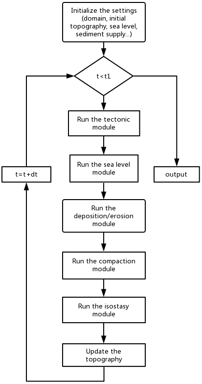
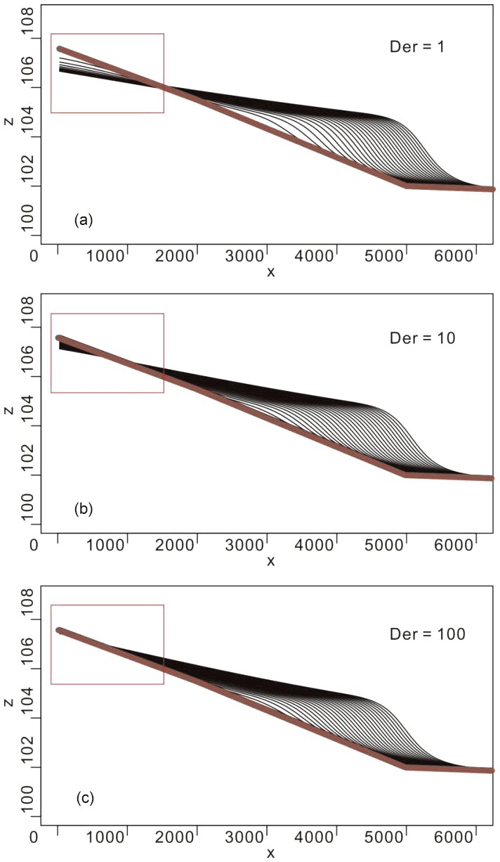
Figure 2 Dip direction section with different Der values (a: Der=1; b: Der=10; c: Der=100). Erosion will be switched off if Der is large enough.

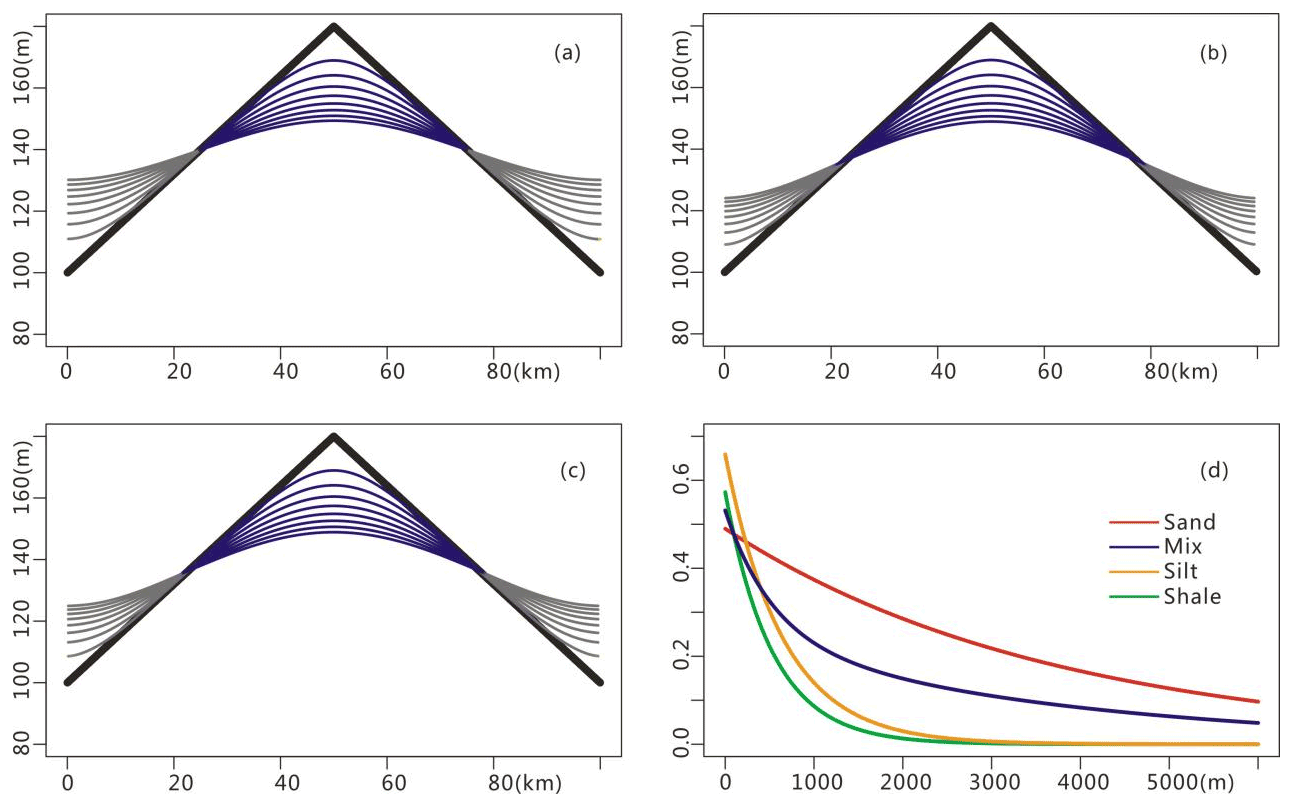
Figure 3 Customized compaction and the porosity curves: (a) the x–z plot with the original depth–porosity scale, (b) the x–z plot with a magnified depth–porosity scale (×100) to enhance compaction, (c) the x–z plot with a magnified depth–porosity scale (×1000) to enhance compaction, (d) depth–porosity curves used in the compaction module (the mix indicates mixed 50 %–50 % sand and shale; for details, see Athy, 1930; Sclater and Christie, 1980).

2 Methodology

2.1 Mathematical model

The Sedapp mathematical model can be expressed as follows:

$$\begin{array}{}\text{(2)}& {\displaystyle }& {\displaystyle }{F}_i{\displaystyle \frac{\partial h}{\partial t}}=\max \left(\mathrm{\nabla }\cdot \left({\mathrm{\Gamma }}_i\mathrm{\nabla }h\right),{\displaystyle \frac{\mathrm{1}}{\mathrm{Der}}}\mathrm{\nabla }\cdot \left({\mathrm{\Gamma }}_i\mathrm{\nabla }h\right)\right)+q\text{(3)}& {\displaystyle }& {\displaystyle }\sum _i^n{F}_i=\mathrm{1},\end{array}$$

where F_i is the fraction of the ith class of sediment, h is elevation, t is time, ∇ is the nabla operator, Der is a user-defined parameter denoting the ratio of deposition to erosion (it can be a scalar, vector or tensor value depending on its temporal and spatial variability), Γ_i is the diffusion coefficient for the ith class of lithology, and q is the source term that is a function of coordinates and time. The source term is used only for endogenetic sedimentation, especially carbonates. If endogenetic sedimentation is ignored, the source term can be left out. Of these, h and F_i are the primary unknowns.

Note that Γ_i cannot be outside the parentheses because it is not constant but instead a function of spatial coordinates and time. Γ can generally be expressed as follows:

$$\begin{array}{}\text{(4)}& {\displaystyle }{\displaystyle }\mathrm{\Gamma }=max\left(\mathit{\alpha }{e}^{-\frac{D(\mathit{x},h,\text{sl}{)}^{\mathit{\eta }}}{\mathit{\beta }}},{\mathit{\alpha }}_{\text{wd}}{e}^{-\frac{\text{Wd}(\mathit{x},h,\text{sl}{)}^{{\mathit{\eta }}_{\text{wd}}}}{{\mathit{\beta }}_{\text{wd}}}}\right)+\mathit{\epsilon },\end{array}$$

where $\mathit{\alpha }/{\mathit{\alpha }}_{\text{wd}}$ are pre-exponential factors (L² T⁻¹), $\mathit{\eta }/{\mathit{\eta }}_{\text{wd}}$ are distance indexes (no dimension), $\mathit{\beta }/{\mathit{\beta }}_{\text{wd}}$ are spatial scale factors (L^η or ${\mathrm{L}}^{{\mathit{\eta }}_{\text{wd}}}$) and ε is an adjustment factor (L² T⁻¹) reflecting the environment energy. In particular, the distance function $D=D(x,h,\text{sl})$ and water depth function $\text{Wd}(x,h,\text{sl})$ change with spatial coordinates x, topography h and sea level sl, and they are applicable to the marine portion only.

When Der=1 and n=2, the 3D (actually 2DH because h is another dimension perpendicular to x and y) scenario for Eqs. (2) and (3) can be expressed as follows:

$$\begin{array}{}\text{(5)}& {\displaystyle }& {\displaystyle }F{\displaystyle \frac{\partial h}{\partial t}}={\displaystyle \frac{\partial }{\partial x}}\left({\mathrm{\Gamma }}_{\mathrm{1}}{\displaystyle \frac{\partial h}{\partial x}}\right)+{\displaystyle \frac{\partial }{\partial y}}\left({\mathrm{\Gamma }}_{\mathrm{1}}{\displaystyle \frac{\partial h}{\partial y}}\right)+q(x,y,t),\text{(6)}& {\displaystyle }& {\displaystyle }\left(\mathrm{1}-F\right){\displaystyle \frac{\partial h}{\partial t}}={\displaystyle \frac{\partial }{\partial x}}\left({\mathrm{\Gamma }}_{\mathrm{2}}{\displaystyle \frac{\partial h}{\partial x}}\right)+{\displaystyle \frac{\partial }{\partial y}}\left({\mathrm{\Gamma }}_{\mathrm{2}}{\displaystyle \frac{\partial h}{\partial y}}\right)+q(x,y,t),\end{array}$$

where x and y are spatial coordinates. This is especially suitable for cases dealing only with two classes of sediments for simplicity, where Γ₁ is the transport coefficient for sand and Γ₂ is the transport coefficient for mud.

For 2D (1DH) scenarios, especially along the section line through the river mouth, the distance-related term is generally larger than the water-depth-related term, and thus the latter term within the max function in Eq. (4) is usually omitted. For convenience in coding and also ignoring the endogenetic sedimentation, Eqs. (5), (6) and (4) can be simplified into

$$\begin{array}{}\text{(7)}& {\displaystyle }& {\displaystyle }F{\displaystyle \frac{\partial h}{\partial t}}={\displaystyle \frac{\partial }{\partial x}}\left({\mathrm{\Gamma }}_{\mathrm{1}}{\displaystyle \frac{\partial h}{\partial x}}\right),\text{(8)}& {\displaystyle }& {\displaystyle }\left(\mathrm{1}-F\right){\displaystyle \frac{\partial h}{\partial t}}={\displaystyle \frac{\partial }{\partial x}}\left({\mathrm{\Gamma }}_{\mathrm{2}}{\displaystyle \frac{\partial h}{\partial x}}\right),\text{(9)}& {\displaystyle }& {\displaystyle }{\mathrm{\Gamma }}_i={\mathit{\alpha }}_i\cdot e^{-\frac{{\left(c\cdot D(\mathit{x},t)\right)}^{\mathrm{2}}}{E}}+\mathit{\epsilon },i=\mathrm{1},\mathrm{2}.\end{array}$$

The joint effect of c and E in Eq. (9) is equivalent to that of β in Eq. (4). The variable c here, with a dimension of L⁻¹, is mainly used to facilitate the scale of distance and differentiate the transport characteristics of different sediment types (e.g., sand and mud). E is a denominator of an exponent. Its corresponding numerator is a transformed distance term, which could be regarded as a proxy to the river-injection-related hydraulic energy. In order to make the whole exponent dimensionless, the denominator and the numerator should have the same dimension. Thus, E could be considered “hydraulic characteristic energy”. While for ε it does not contribute very much to the deposition geometry around the shoreline, it could significantly affect the sedimentation deep in the basin. This seems to have little to do with the transportation capability originating from the river injection, instead the most appropriate description is as the energy inherent in the basin that carries the sediments to the basin center.

2.2 Code implementation

Sedapp was written in the R language and its solution was based on the finite volume method (FVM), which has the desired property of local mass conservation and has a clear physical meaning (Versteeg and Malalasekera, 2007; Moukalled et al., 2016; P. Liu et al., 2017). The cell-centered variable arrangement method was used to store the unknowns at the grid element centroids. The nonlinearity was implemented through stepwise iteration (Fig. 1).

The brief workflow within a single time step is as follows:

1. implement user-defined tectonic subsidence and update the topography;

2. implement user-defined sea level and identify and update the shoreline location;

3. solve the differential deposition and erosion function;

4. implement the compaction and isostatic subsidence.

Step 3 is an important step. According to the hypothesis of diffusion-based FSM models, the change rate (by either deposition or erosion) is proportional to the gradient of the slope (Fernandes et al., 1997; Pelletier, 2013). If we use the diffusion equation and law directly without any differential treatments between deposition and erosion (in other words, Der is held at 1), it will be very difficult to treat some complex situations. For example, some bed surface is “hard ground”, which is very difficult to erode, whereas the overlying deposition process is relatively easy. Hence, for a given location, erosion and deposition could occur at different rates, and Der may not be equal to 1. For example, if we wanted the erosion rate to be only $\mathrm{1}/\mathrm{100}$ of the deposition rate, Der can be set to 100. Using the max() function in Eq. (2) for a deposition process (namely the $\frac{\partial h}{\partial t}>\mathrm{0}$), ∇⋅(Γ_i∇h) would be larger than $\frac{\mathrm{1}}{\text{Der}}\mathrm{\nabla }\cdot \left({\mathrm{\Gamma }}_i\mathrm{\nabla }h\right)$ and ∇⋅(Γ_i∇h) is used. Otherwise, $\frac{\mathrm{1}}{\text{Der}}\mathrm{\nabla }\cdot \left({\mathrm{\Gamma }}_i\mathrm{\nabla }h\right)$ is used. If a non-erosion case is desired, Der can be set to a very large value.

Generally, sediment supply rate cannot be directly defined through boundary condition settings since the latter can only determine the boundary slope. Therefore, Sedapp uses a negative-feedback strategy to define the sediment supply rate. At each time step, the total amount of deposition within a step is first calculated using the previously defined α_test and then the adjusted α_mod is calculated by Eq. (10):

$$\begin{array}{}\text{(10)}& {\displaystyle }{\displaystyle }{\mathit{\alpha }}_{\text{mod}}={\mathit{\alpha }}_{\text{test}}{\displaystyle \frac{V_{\text{expected}}}{V_{\text{test}}}},\end{array}$$

where α_mod denotes the modified α of this time step, V_expected denotes the expected sediment increment, namely the sediment supply rate, and V_test denotes the computed sediment increment with α_test.

Figure 4 Typical stacking patterns acquired through different sea level change rates.

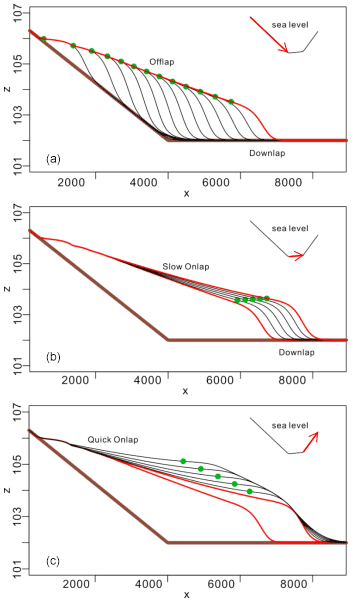
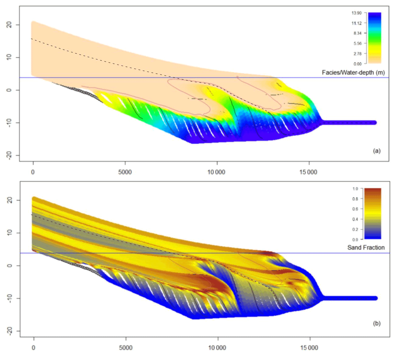
Figure 5 Simulated stratigraphy under two full sea level cycles: (a) facies section and (b) lithological section.

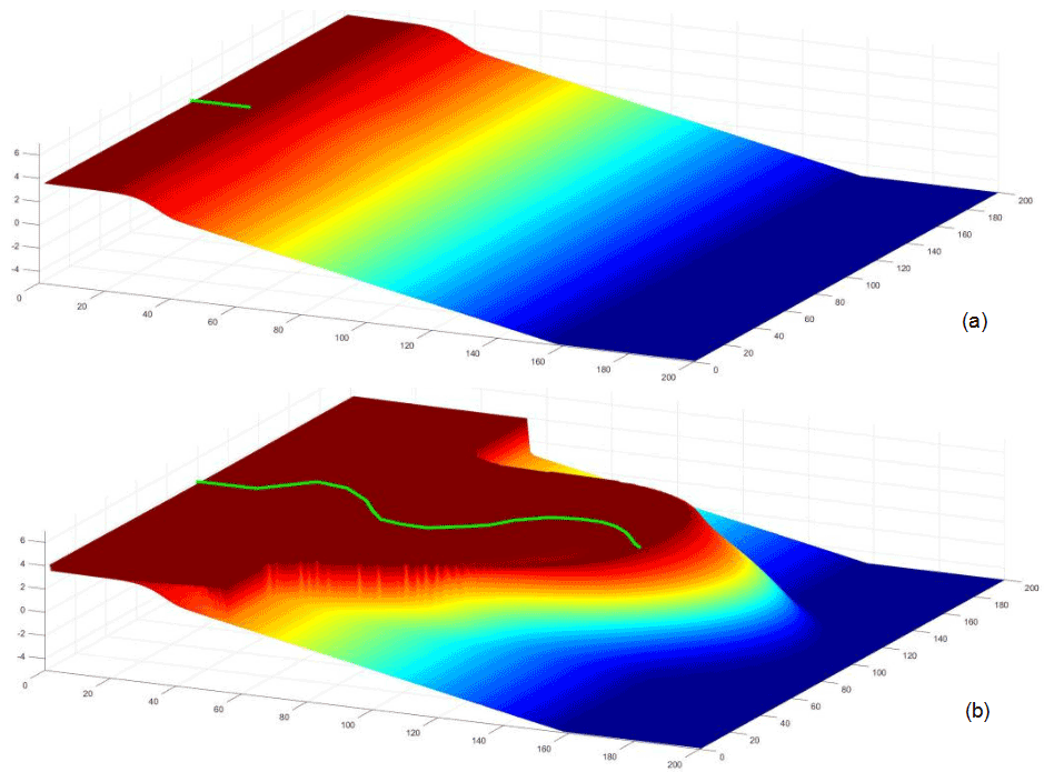
Figure 6 The initial topography and the simulated results of Model 1: (a) the initial topography and (b) the topography at t=10 Myr.

Table 1 The main simulation parameters of Model 1 (see Sect. 2.1 an explanation of the notation).

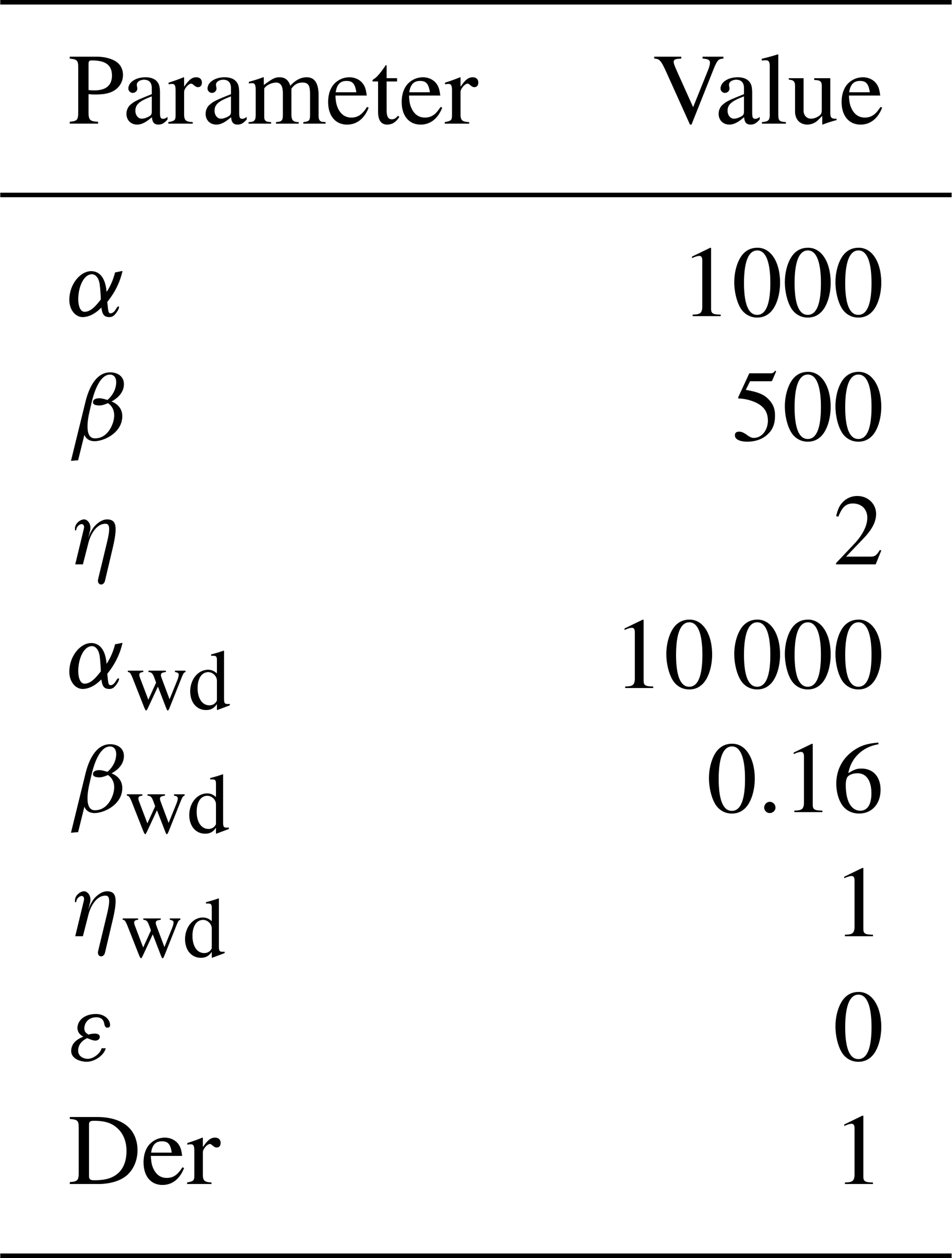
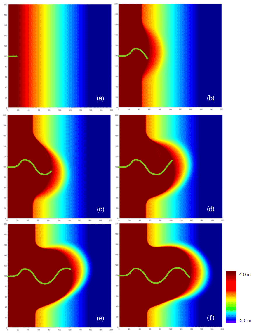
Figure 7 Plane view of Model 1 results: (a) t=0 Myr, (b) t=2 Myr, (c) t=4 Myr, (d) t=6 Myr, (e) t=8 Myr and (f) t=10 Myr.

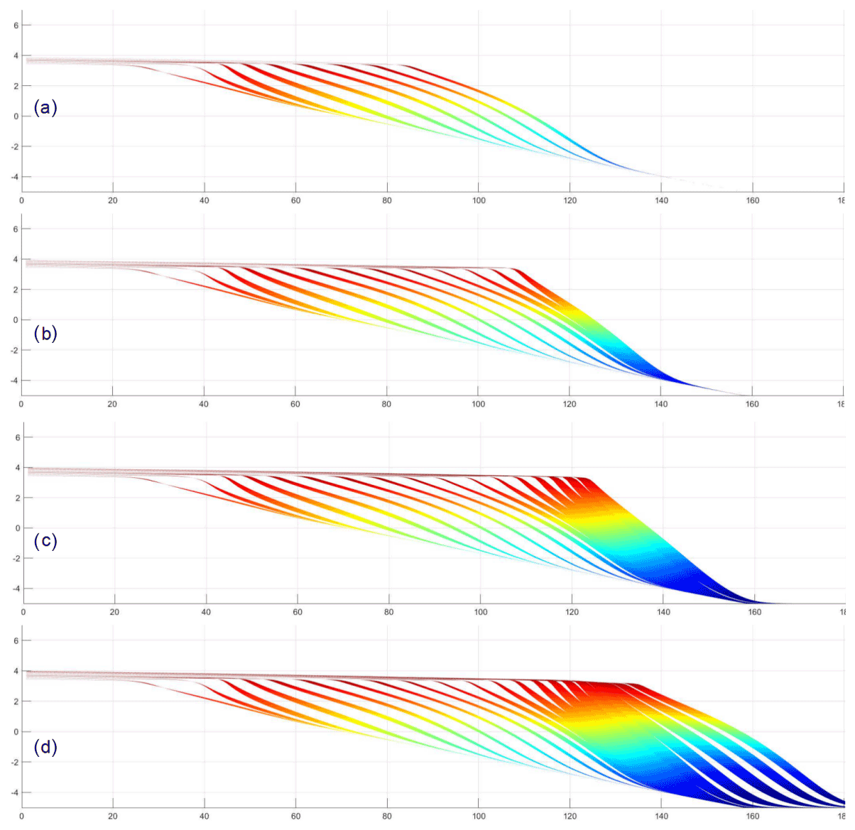
Figure 8 Cross section at x=75 m: (a) t=4 Myr, (b) t=6 Myr, (c) t=8 Myr and (d) t=10 Myr. The blank spaces divide the strata into isochronous stratigraphic units, which can be used to infer the relative deposition rate.

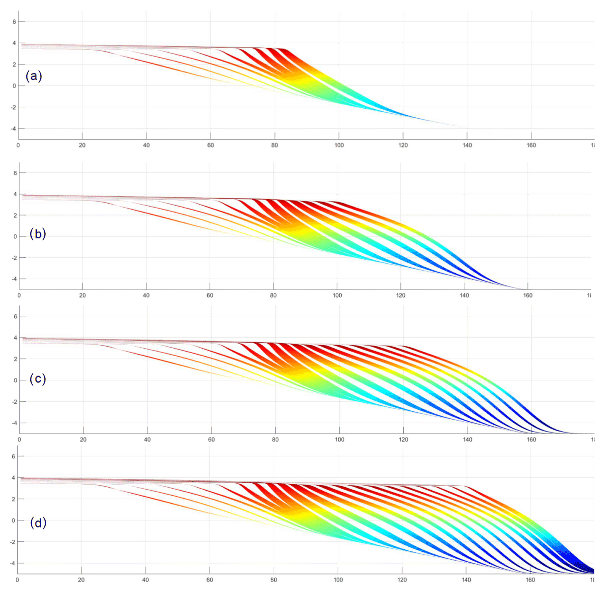
Figure 9 Cross section at x=125 m: (a) t=4 Myr, (b) t=6 Myr, (c) t=8 Myr and (d) t=10 Myr. The blank spaces divide the strata into isochronous stratigraphic units, which can be used to infer the relative deposition rate.

Figure 10 The Horton River delta in Canada (a) and the Ebro delta in the Mediterranean Sea (b) (taken from © Google Maps).

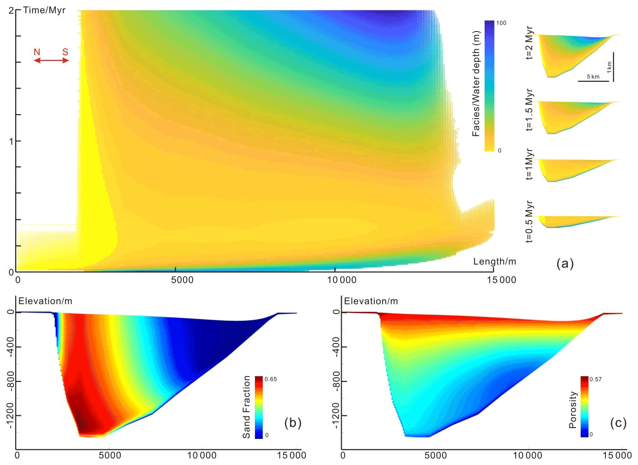
Figure 11 Simulation results of Gaobei Slope Belt during the study interval: (a) Sedapp results of facies in the time domain (Wheeler diagram) and depth domain at different times, (b) Sedapp results of sand fraction in the depth domain, and (c) Sedapp results of porosity in the depth domain.

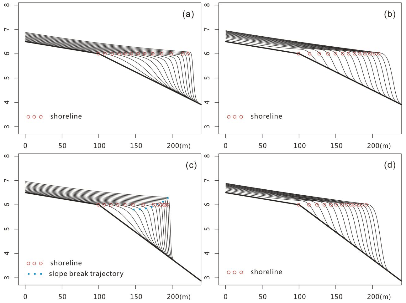
Figure 12 Comparison of the simulated results from a water-depth-based algorithm and the algorithm of Sedapp: (a) clinoforms of gentle slopes created in water depth models, (b) clinoforms of gentles slope created in Sedapp, (c) clinoforms of steep slopes created in water depth models and (d) clinoforms of steep slopes created in Sedapp. The results of the two algorithms did not diverge strongly when the original slope was gentle, while the clinoform shapes and slope break trajectories could be very different when the slope was steep.

3 Characteristics

3.1 Nonlinear transport coefficients

The nonlinear transport coefficient is a feature of Sedapp. Sedapp's transport coefficient uses a function of both the distance from the estuary and the water depth. This feature makes it easier to simulate fluvial and deltaic processes in 2DH scenarios, which can reflect changes along the shore. Even in 1DH cases, this feature also has some advantages (see Sect. 5 for details).

Generally, a smaller c value in Eq. (9) results in a higher sediment travel distance and a larger distribution range when the total amount of sediment is fixed. For example, the c value of mud is usually set to 50 %–85 % of sand, reflecting the differential deposition of sand and mud. In addition, the environment energy ε can also influence the sediment travel distance. For example, a larger ε will make the sediment travel further. As sedimentation progresses, the position of the estuary may change, and thus the distance from the estuary is updated at each time step to achieve the nonlinearity of Γ.

3.2 Differential and customizable deposition/erosion rate

During the actual deposition process, the properties of the underlying strata (such as compaction degree, lithology and age), as well as some external environmental factors (such as temperature, humidity and pH value), will affect the erosion rate. Therefore, the customized treatment of erosion rate is another Sedapp characteristic.

In Sedapp, the deposition rate is a parameter that can be specified directly (for the adjustment process see Sect. 2.2). Furthermore, the Der parameter is a user-defined parameter that controls the ratio of deposition rate to erosion rate. When Der is 1, the deposition rate is equal to the denudation rate (Fig. 2a), and when Der value is 10 or 100, denudation is significantly weakened (Fig. 2b). Theoretically, if the value of Der is large enough, it is equivalent to completely eliminating the denudation effect. Der values should be customized according to the actual situation.

3.3 Customizable compaction

Compaction is an important geological process after sediment deposition, especially when the sediment thickness is very high. In Sedapp, the compaction process can be easily realized by setting the composition of lithology and porosity curves.

In this paper, we designed a pyramid-shaped mountain simulation commonly used by other researchers (as shown in Fig. 3; see Rivenaes, 1992, and Yuan et al., 2019, for reference). The Der value was set to 1. The sediment supply ratio of sand and mud was set to 1:1, and the porosity curve was set as shown in Fig. 3d. After simulation, the top of the pyramid was denuded and the foot of the pyramid had deposited sediment of a given thickness.

To illustrate the effect of compaction, Sedapp introduces a scale factor that can enlarge the longitudinal scale. Figure 3a shows the original compression scale (that is, the scale factor was equal to 1), and the scale factors in Fig. 3b and c were 100 and 1000, respectively. It can be seen that sediment thickness at the foot of the pyramid in Fig. 3c was significantly smaller than that in Fig. 3a. The factors that caused these differences were not only depth but also the proportion of sand and mudstone and the shape of depth–porosity curves, which can be easily adapted to different scenarios by modifying the lithologic proportion and porosity–depth functions in Sedapp.

4 Verification of Sedapp

To identify how well the algorithm works within geological context, some simple benchmark simulations are given below.

4.1 Typical stacking patterns

Typical stacking patterns, including forced regression, normal regression, and transgression can be formed (Fig. 4) by fixing sediment supply while controlling the adjusted sea level rise rate.

During the period of sea level decline, the shoreline moved seaward, and the onlap points also moved seaward to form the offlap and downlap stratigraphic termination structures (Fig. 4a). During slow sea level rise, the shoreline continued to move seaward, but the onlap points started to move landward, forming an onlap termination structure. At the other end, the downlap structure continued to exist. During rapid sea level rise, the shoreline started to move landward, and the onlap points also moved landward. At this time, the downlap structure did not exist above the slope break but may have existed below the slope break.

4.2 Typical two-cycle scenario

To demonstrate the complete base level changing process, this paper designed a simulation with two full sinusoidal cycles as shown in Fig. 5. In the first cycle, the shoreline dropped and moved seaward. Then it slowly rose and gradually moved landward until it reached the highest point and tended to stabilize. The water depth of deposition in the strata gradually deepened from left to right on the marine side (Fig. 5a), and the sandy content reached a maximum around the shoreline (Fig. 5b) near the shoreline. In the strata on the land side, the sand content was stratified. The sand content was relatively large during the early transgression and subsequently relatively small. The second cycle was located above the first cycle and continued the same characteristics as the first cycle, but the deposition range was enlarged and the average single layer thickness was thinner.

4.3 Case studies

Model 1

In order to better display the 2DH performance of Sedapp, this paper designed Model 1. Its length and width ranges were both 200 m, and the elevation range was about 10 m. The mesh was 200×200 in x–y plane. The time span of the model was set at 10 Myr, and the step size was set at 0.5 Myr. Sea level was kept constant at 3 m. The initial topography was set as shown in Fig. 6a. A river was set up in the central position of the y axis (y=100 m). The channel shape of the river was set in advance as a sine curve. The fluvial profile slope was set to a constant of 0.00357, and the sediment supply rate was not defined since it could vary according to the fluvial profile slope. The other main parameters of the model are shown in Table 1.

Projection of the simulation results on the x–y plane clearly showed the variability along the shore (Fig. 7). When t=0, the shoreline was a straight line, and the channel was in the middle of the shoreline. As time went on, the river mouth continued to move forward. From 0 to 2 Myr, the channel first swung to the north, then to the south and finally the shoreline began to bulge slightly towards the sea side. From 2 Myr, the channel continued to swing southward, until the time approached 4 Myr and the river mouth began to slowly turn north. From 4 to 6 Myr, the channel continued to swing northward, and the convex part towards the sea side became more prominent. From 6 to 8 Myr, the channel continued the previous trend, while the convex shoreline became asymmetrical (increasing skewness to the north). From 8 to 10 Myr, the principal line of the channel moved southward, and the convex shoreline gradually returned to being symmetrical (Fig. 7).

The simulation results also revealed some interesting features in longitudinal sections (Fig. 8). Two sections (y=75 m and y=125 m) perpendicular to the shoreline direction were selected (see Fig. 7f for the position of the section line). The two sections are located on the north and south sides of the main channel. The distance between the channel and the two sections was variable. In the southern profile (y=75 m), from 4 to 10 Myr, the isochronous lines of the formation changed from sparse to dense and then from dense to sparse (i.e., the thickness of a single clinoform changed first from thick to thin and then from thin to thick) (Fig. 8). This was completely contrary to what was observed in the northern profile (y=125 m). From 4 to 10 Myr, the isochronous lines first changed from dense to sparse and then from sparse to dense, reflecting that the deposition rate first increased and then decreased (Fig. 9).

Under the parameters shown in Table 1, due to the existence of estuaries, the shoreline bulged towards the sea side. A closer distance to the river mouth would result in a higher sedimentation rate and a greater shoreline advancing speed. From 2 Myr, the convex shape of the shoreline towards the sea side became more apparent, similar to the morphology of some real-world deltas (Fig. 10).

Model 2

This code can be applied not only to marginal marine environments but also to the continental fault basins. Taking the three- and four-sand groups of the third member of Shahejie Formation in the Gaobei slope belt of Nanpu Sag in Bohai Bay basin as an example, we conducted a simplified 1DH real case study. The basic geological background is as follows: during the deposition period of this set of strata, the normal fault tectonic movement in the north of the sag was active, which was the main controlling factor leading to the increase of accommodation space. At the same time, the terrigenous clasts that came from the north were sufficient, and the basin was in a balanced state (Li et al., 2018). According to the geological background, a simplified reconstruction model (Model 2) was designed that assumed that the subsidence rate of the boundary fault and sediment supply rate is constant, neglected the effect of isostasy and considered the effect of sediment compaction.

The simulation results are shown in Fig. 11. From the perspective of temporal and spatial stratigraphy, the shoreline mainly moved towards the sag center during the early stage and then moved back to the land side. The deepest water depth occurred in the middle southern part at 2 Myr (Fig. 11a). This shoreline phenomenon is usually called auto-retreat (Muto and Steel, 2002). The sand fraction section shows that the steep slope belt in the north was richer in sand content than the south (Fig. 11b). The porosity section shows that porosity generally decreased from bottom to top. The porosity also varied horizontally, especially when the depth was greater than 800 m. The porosity in the north was higher than in the south.

Due to the oversimplified assumptions, the simulation results would not necessarily be consistent with every practical borehole. However, the simulation revealed general trends that can strengthen or improve our existing understanding and validate the previously proposed conceptual model.

5 Discussion

Sedapp is a diffusion-based model, and its transport coefficient is a function of both distance from estuary and water depth. Compared with most existing diffusion models based only on water depth, this modification has great advantages in fluvial–deltaic environments, especially for 2DH scenarios. Sedapp not only simulates some surface landscapes, but it also reveals some interesting internal features. In the sections beside the channel in Model 1, the formation rate of the clinoforms had a close relationship with distance between the channel and the section. This may be of great significance for analyzing ancient strata. Considering the resolution of seismic data, it is easier to observe changes in the density of the foreset than to directly find a channel. This may provide some an supplement to the data in areas with less borehole data. Sedapp also showed strong simulation ability in 1DH scenarios. It can avoid some potential problems that water depth models may not overcome. For example, when the slope is steep, the slope break trajectory created by the water depth model can even end up far above the shoreline (Fig. 12a and c). In contrast, Sedapp does not face such a problem. As long as the sea level is constant, the slope break line will remain in a straight line and the clinoforms will also move smoothly to the ocean (Fig. 12b and d).

Sedapp can be used not only in shallow marine environments but also in continental fault basins (Fig. 11). In the case of Model 2 (Sect. 4.3), the simulation results of this study were very similar to those of the previous study (Li et al., 2018). In Li et al. (2018), the results were generated by Sedpak, an FSM model widely used in continental fault basins. Both Sedapp and Sedpak performed well in this case despite their core algorithms being different. Compared with the diffusion-based Sedapp, Sedpak is mainly geometry based. Various geometric rules (e.g., alluvial angles, submarine angles, bypass angles) govern the processes in Sedpak. To generate a simple clinoform, setting a transport coefficient is apparently more convenient than designing the above angles. This is an advantage of Sedapp over Sedpak for beginner users. Another advantage of Sedapp over Sedpak is its flexibility in graphing. For example, the relative content of sand can only be expressed by discrete yellow and green belts in Sedpak, while in Sedapp it is more flexible. A continuous color bar is available, and the sand fraction can be expressed in a variety of ways due to its open-source nature.

The transport coefficient is a relatively long-term geomorphologic physical quantity, while wave, tidal and current energy are relatively short-term hydrodynamic quantities. However, they are closely related. A river entering the sea is a type of jet flow phenomenon. The flow velocity decreases rapidly from the river mouth to the sea, which also has a strong negative correlation with the distance to the mouth of the river. The contour map of water flow velocity is fan shaped. At the same time, the decrease of velocity is also an important cause of sediment deposition, which also explains the close fan-shaped morphology of a delta front. Correspondingly, an increase in water depth will also decrease the flow velocity. For the open coast without river injection, a model based on water depth seems to be reasonable. However, for a coast with river injection, it is difficult to explain the formation of the fan-shaped morphology of a delta. Therefore, it can be concluded that (in more general cases) the transport coefficient should be a function of short-term water energy, which is related to both the estuary distance and the water depth. When there is river injection, the river process is dominant and the estuary distance function is a reasonable proxy for the transport coefficient. When there is no river injection, the water depth plays the main role. In addition, particle size is also a decisive factor (Nash 1980; Andrews and Bucknam, 1987). Hence, a choice function (see Eq. 9) and differentiated α are used to adapt different environments and lithologies. Although the current results of Sedapp seem plausible, these settings for the transport coefficient are still empirical. Due to the complex nature of the transformation from short-term processes to long-term ones, it is difficult to build an accurate bridge between sediment hydrodynamics and stratigraphic formation, which may be the focus of the next step.