the Creative Commons Attribution 4.0 License.
the Creative Commons Attribution 4.0 License.
 | 24 Jun 2021
Understanding each other's models: an introduction and a standard representation of 16 global water models to support intercomparison, improvement, and communication
Camelia-Eliza Telteu
Hannes Müller Schmied
Wim Thiery
Guoyong Leng
Peter Burek
Xingcai Liu
Julien Eric Stanislas Boulange
Lauren Seaby Andersen
Manolis Grillakis
Simon Newland Gosling
Yusuke Satoh
Oldrich Rakovec
Tobias Stacke
Jinfeng Chang
Niko Wanders
Harsh Lovekumar Shah
Tim Trautmann
Ganquan Mao
Naota Hanasaki
Aristeidis Koutroulis
Yadu Pokhrel
Luis Samaniego
Yoshihide Wada
Vimal Mishra
Junguo Liu
Petra Döll
Fang Zhao
Anne Gädeke
Sam S. Rabin
Florian Herz
Global water models (GWMs) simulate the terrestrial water cycle on the global scale and are used to assess the impacts of climate change on freshwater systems. GWMs are developed within different modelling frameworks and consider different underlying hydrological processes, leading to varied model structures. Furthermore, the equations used to describe various processes take different forms and are generally accessible only from within the individual model codes. These factors have hindered a holistic and detailed understanding of how different models operate, yet such an understanding is crucial for explaining the results of model evaluation studies, understanding inter-model differences in their simulations, and identifying areas for future model development. This study provides a comprehensive overview of how 16 state-of-the-art GWMs are designed. We analyse water storage compartments, water flows, and human water use sectors included in models that provide simulations for the Inter-Sectoral Impact Model Intercomparison Project phase 2b (ISIMIP2b). We develop a standard writing style for the model equations to enhance model intercomparison, improvement, and communication. In this study, WaterGAP2 used the highest number of water storage compartments, 11, and CWatM used 10 compartments. Six models used six compartments, while four models (DBH, JULES-W1, Mac-PDM.20, and VIC) used the lowest number, three compartments. WaterGAP2 simulates five human water use sectors, while four models (CLM4.5, CLM5.0, LPJmL, and MPI-HM) simulate only water for the irrigation sector. We conclude that, even though hydrological processes are often based on similar equations for various processes, in the end these equations have been adjusted or models have used different values for specific parameters or specific variables. The similarities and differences found among the models analysed in this study are expected to enable us to reduce the uncertainty in multi-model ensembles, improve existing hydrological processes, and integrate new processes.
- Article
(995 KB) - Full-text XML
-
Supplement
(3156 KB) - BibTeX
- EndNote
- Included in Encyclopedia of Geosciences


Many multi-model intercomparison projects (MIPs) have been designed to provide insights into various Earth system processes. They provide many multi-model ensembles consisting of multiple models driven by the output of multiple other models. These multi-model ensembles offer the opportunity to inter-compare models for an improved understanding of process representation and inter-model differences as well as for model improvement. Some MIPs examples include FireMIP for the fire regime and its drivers (Rabin et al., 2017); CMIP for past, present, and future climate changes and their drivers (Eyring et al., 2016; Kageyama et al., 2018); LakeMIP for physical and biogeochemical processes of lakes (Stepanenko et al., 2010; Thiery et al., 2014); AgMIP for crop growth (Rosenzweig et al., 2013); and WaterMIP or ISIMIP for the water cycle (Haddeland et al., 2011; Frieler et al., 2017).
MIPs have encountered many challenges as to how to inter-compare models and interpret various model results (von Lampe et al., 2014), realize the standardization of data and scenarios and integrate transdisciplinary knowledge in modelling (Rosenzweig et al., 2013), and identify and reduce uncertainties (Sitch et al., 2008). They have been affected by scientific complexity, input data quality, technical infrastructure, and even cultural and organizational challenges (Eyring et al., 2016). Hence, they have evaluated model performance in the past and have focused on inter-model agreement for the future. Ultimately, MIPs and their multi-model ensembles have been blocked from interpreting inter-model differences because of model complexity, missing information about other models, incomplete or missing information about heterogeneity, and dynamism of natural systems (M. P. Clark et al., 2011).
Nevertheless, MIPs have underlined the need to go beyond good overall model performance and to improve process representation in the models (Guseva et al., 2020), integrate missing processes (Friend et al., 2014), and reduce uncertainties (Warszawski et al., 2014). MIPs showed that robust similarities exist among models, and as a result models are not strictly independent of each other given previous and legacy versions, and there are existing links among modelling communities who indirectly transfer some models' strengths and weaknesses by sharing their ideas and codes (Masson and Knutti, 2011; Knutti et al., 2013). It has been demonstrated that there is no perfect model (Essery et al., 2013; Ullrich et al., 2017) and that there is a need to understand better how different models work.
Thereby, the modelling communities are still testing and learning how to improve modelling and how to realize multi-model inter-comparison studies. However, few studies have undertaken model experiments on process representation and evaluated the models for specific events or characteristics specifically on the catchment scale (de Boer-Euser et al., 2017; Duethmann et al., 2020; Bouaziz et al., 2021). Furthermore, some studies have tested how model equations combined in different configurations and using different parameter values influence the simulations, e.g. Essery et al. (2013) (testing 1701 snow model configurations), Niu et al. (2011) (Noah-MP model), Pomeroy et al. (2007) (Cold Regions Hydrologic Model, CRHM), and Kuppel et al. (2018) (Ecohydrologic model, EcH2O). In summary, they found that some model configurations provide consistently good results, others provide consistently poor results, and many configurations provide good results in some cases and poor results in others (Essery et al., 2013).
In this complex scientific context, the present study represents a step forward toward advancing the understanding of process representation and inter-model differences within one large MIP, specifically, ISMIP – the Inter-Sectoral Impact Model Intercomparison Project (Frieler et al., 2017). We assessed the equations applied by 16 state-of-the-art global water models (GWMs) to simulate the vertical and lateral water balance and human water use sectors on the global scale. We created a standard writing style for these equations to identify similarities and differences among models. Our goal is to provide the global water community with an overview of the model structures and the basis required to interpret various model results and to design future experiments on how model equations, model configurations, and model parameter values influence the model outputs.
The three main objectives of the study are as follows:
-
to provide a better understanding of how 16 state-of-the-art global water models are designed;
-
to show similarities and differences among them, based on their equations;
-
to underline future research potential in global water modelling.
Essentially, this study supports intercomparison, improvement, and communication among 16 modelling teams. It also provides the basis for (i) further water model (inter-)comparison studies, including model outputs, (ii) selecting the right model(s) for a given application, and (iii) identifying data needs for a given analysis and application. We believe that two considerations are useful in the interpretation of model results: (i) knowing model structures and (ii) identifying the effect of model structures on model results. The present study is focused only on the first consideration because understanding model configurations is needed to interpret various model results.
Our target audience includes students, junior and senior scientists, and modellers (or people who want to become modellers). Furthermore, this study could be used by stakeholders or other people who want to understand the background of global water models and how they simulate the global freshwater system. We present the modelling approaches and terminology used in global water modelling in Sect. 2. In Sect. 3, we present key characteristics of the models analysed in the present study. In Sect. 4, we describe our standard writing style of model equations. In Sect. 5, we present similarities and differences among models. In Sect. 6, we present the number of water flows, water storage compartments, and human water use sectors included in the 16 GWMs. In Sect. 7, we discuss potential future research in global water modelling. Finally, in Sect. 8, we present recommendations for future multi-model intercomparison projects and extended assessments.
2.1 Differences in modelling approaches
On global scale, the terrestrial water cycle is simulated by three different communities that have developed three types of models: (i) the climate community that has developed land surface models (LSMs), (ii) the global hydrological community that has developed global hydrological models (GHMs), and (iii) the vegetation community that has developed dynamic global vegetation models (DGVMs). In this study, the land surface models are CLM4.5, CLM5.0, DBH, JULES-W1, MATSIRO, and ORCHIDEE. The global hydrologic models are CWatM, H08, Mac-PD20, mHM, MPI-HM, PCR-GLOBWB, VIC, WaterGAP2, and WAYS. One model (LPJmL) is a dynamic global vegetation model.
However, these three communities focus on specific hydrological and atmospheric processes, as well as anthropogenic impacts. These key aspects are important for their specific research, leading to different modelling approaches, specific evaluation studies of model performance (Archfield et al., 2015), and different field-specific meanings of terminology used (Beven and Young, 2013). Thus, combining the expertise in their key aspects would create a strong synergy and improve the models of these communities, but for this goal they have to interact with each other, identify their similarities and differences, and share experiences. They need to undertake joint experiments, share and discuss their results, and discuss how they influence and depend on each other and how water modelling can be improved (Cucchi et al., 2020).
The global hydrological community focuses primarily on surface water and groundwater availability, its human interference, and the changes of the water cycle. GHMs simulate the water cycle with its water flows, water compartments, and human water use sectors. These models simulate water abstracted for the irrigation, domestic use, livestock, industry (manufacturing and electricity), and desalination sectors. Furthermore, reservoir management and its streamflow alteration are included. One of their main foci is streamflow simulation and their ability to reproduce historical observations of this variable. They focus on lateral and vertical flows, comprehensively simulating the following surface water bodies: (i) lakes, (ii) wetlands, (iii) rivers.
The climate community focuses on simulating climate and its change over decades and centuries using global climate models (GCMs) and Earth system models (ESMs). A fundamental component of these are the LSMs, which simulate the water and energy exchanges between the land surface and the atmosphere, specifically focusing on vertical flow exchanges. Therefore, these models simulate the energy cycle, the water cycle, the carbon and nitrogen cycles, and vegetation and crop responses to temperature, precipitation, and CO2 concentrations. Further, they represent the soil with a higher vertical resolution and evapotranspiration and snow dynamics in a more physical manner than the global hydrological models (GHMs; Döll et al., 2016; Pokhrel et al., 2016; Wada et al., 2017).
The vegetation community focuses on vegetation distribution and growth in an area and over a time interval and is primarily interested in the global carbon cycle. DGVMs simulate shifting vegetation, driven by biogeochemistry, hydrology, and anthropogenic influences. These models simulate the vegetation composition and distribution as well as compartments and flows of carbon and water, for both natural and agricultural ecosystems. Specifically, they model the active response of vegetation to changes in air temperature, precipitation, and CO2 concentrations.
The different viewpoints of these communities are readily visible in very basic concepts such as the solar energy. This is the main driver that connects the processes of terrestrial water cycle simulated by these communities. It specifically links the water and energy budgets with vegetation processes. This link can be exemplified by the latent heat flux of evaporation that describes the heat or the energy required to change the liquid water into water vapour. This heat or energy is locked in the humid air as water vapour and is released when the humid air touches cold air and water vapour condensation starts. Therefore, continental evaporation is considered to be water loss by the global hydrological and vegetation modelling communities but a water source (for cloud formation) by the climate community (those that simulate the atmosphere), with implications for agriculture and ecosystems (Abbott et al., 2019). Additionally, transpiration represents a water source for the vegetation community, necessary for photosynthesis and plant growth, and water loss for the global hydrological community.
Overall, these three communities have developed three types of models to simulate the terrestrial water cycle on the global scale despite fundamental differences in model structure, model equations, and output variables. Hence, we decided to include the three types of models in one group and call them global water models (GWMs).
2.2 Definitions used in global water modelling
A global water model describes the dynamic behaviour of a hydrological system that includes input variables, state variables, parameters, constants, and output variables (Bierkens and van Geer, 2007). State variables define how much water is in a compartment or storage at the beginning of the simulation and can change in space and time, for example, soil water storage. Their variation is caused by a variation of the input variables, for example, precipitation. State variables are related to the input variables and output variables through parameters, for example, infiltration capacity of the soil. Parameters and coefficients represent numbers that describe a particular characteristic of reality, of the model, or of the catchment area or flow domain. Some examples are soil porosity, hydraulic conductivity of different soil horizons, maximum soil water storage, maximum canopy water storage, mean residence time in the saturated zone, surface roughness, and vegetation properties (Beven, 2012). A model also uses physical and mathematical constants meaning characteristics of the model that do not change in space and time such as catchment area. Physical constants are physical quantities that can be measured and have a constant value in time, for example, the density of water at 0 ∘C, i.e. the density of ice. Mathematical constants cannot be measured but can be calculated and have a fixed numerical value, for example, e=2.718…, π=3.142. Ultimately, output variables are results of the simulation and vary in space and time, for example, streamflow in a river catchment.
Thus, a global water model includes many equations written with a programming language in a model code to simulate freshwater systems. During simulations, many parameters receive specific values because they cannot be measured everywhere, therefore, they are calibrated or tuned or estimated from auxiliary data that can be measured (such as lookup tables for vegetation properties based on remote sensing observations) to attain the best match between simulated and observed data. The final step of a simulation is to validate (evaluate) simulated model output with observed data through analysis and visualization.
In this study, we analyse 16 state-of-the-art global water models included in the global water sector of the Inter-Sectoral Impact Model Intercomparison Project phase 2b (ISIMIP2b: Frieler et al., 2017). GWMs include six land surface models (LSMs), nine global hydrologic models (GHMs), and one dynamic global vegetation model (DGVM: LPJmL, Tables 6 and 12). These models, as applied within the ISIMIP2b framework, are suitable for application over a catchment size of at least four grid cells (Döll et al., 2003; Hunger and Döll, 2008). For smaller catchments, the results are often not reasonable (e.g. Beck et al., 2016) and require corrections due to inaccurate input data, spatial heterogeneity, and the missing representation of some hydrological processes (Döll et al., 2003; Hunger and Döll, 2008).
3.1 General setup
These models contribute to an experiment setup designed to assess the impact of historical and future warming under the Paris Agreement (Frieler et al., 2017). They are driven by the same climate input datasets under representative concentration pathways (RCPs) and socioeconomic scenarios (SSPs). The time span of the simulations is divided into pre-industrial (1661–1860), historical (1861–2005), and future (RCP2.6, RCP6.0, and RCP8.5, 2006–2099 (2299)). These models simulate the terrestrial water cycle on the global land area (except Antarctica) and quantify water flows, water storage compartments, and human water use under the given climatic and socioeconomic conditions. They do not simulate the ocean component of the global water cycle or water quality. Some of these models also consider reservoir operations.
3.2 Temporal and spatial characteristics
A total of 12 models have a daily temporal resolution (Table 6), while 2 models have a 6-hourly resolution (CLM4.5 and CLM5.0). MATSIRO has an hourly resolution, and ORCHIDEE has 30 min temporal resolution. The 15 models run with a spatial resolution of 0.5∘. ORCHIDEE runs with a spatial resolution of 1.0∘ and has its outputs converted to 0.5∘ spatial resolution. Some models include subgrids for some components: CLM4.5 and CLM5.0 for vegetation, surface runoff, and evapotranspiration; H08 and CWatM for land cover; MPI-HM for surface runoff and evapotranspiration; PCR-GLOBWB for vegetation and land cover; WaterGAP2, CWatM, and MATSIRO for snow; and VIC for vegetation and elevation. Furthermore, MATSIRO divides a subgrid cell into snow-covered and snow-free portions with flows and storages resolved separately for these portions both for land and canopy surfaces.
3.3 River networks used
Nine models (CLM4.5, CLM5.0, CWatM, H08, LPJmL, MATSIRO, MPI-HM, PCR-GLOBWB, WaterGAP2) use the 30 min global drainage direction map DDM30 (Döll and Lehner, 2002), a raster map with a spatial resolution of 0.5∘ × 0.5∘ (∼50 km × 50 km), to outline the drainage directions of surface water collected by creeks, rivulets, and rivers. In this map, 67 420 discrete grid cells are characterized by their specific drainage direction and are organized into drainage basins that drain from the Earth's land surface into the ocean or inland sinks. The mHM uses a river network (0.5∘ × 0.5∘) upscaled from HydroSHEDS (Lehner, 2019). ORCHIDEE uses the river network from the Simulated Topological Networks (STN-30p: Vörösmarty et al., 2000). Five models (DBH, JULES-W1, Mac-PDM.20, VIC, and WAYS) do not use any river-routing scheme for the ISIMIP2b because they do not compute streamflow.
3.4 Calibration approaches for ISIMIP2b
Three GWMs perform calibration of their hydrological components, using different approaches, for ISIMIP2b (Table 6). WaterGAP2 uses a basin-specific approach to match long-term mean annual observed streamflow at the outlet of 1319 river basins. It considers runoff as a nonlinear function of soil moisture and uses a runoff coefficient plus up to two additional factors for calibration (Müller Schmied et al., 2014, 2021). In mHM, calibration of global model parameters is performed against the daily observed streamflow, along with gridded global fields of FLUXNET evaporation (Jung et al., 2011) and a GRACE terrestrial water storage anomaly, using the ERA5 climate forcing (Landerer and Swenson, 2012). WAYS is calibrated against data from the International Satellite Land Surface Climatology Project (ISLSCP) Initiative II of the University of New Hampshire and GRDC composite monthly runoff data (Fekete et al., 2011) from 1986 to 1995 at a 0.5∘ spatial resolution. Seven models (CLM4.5, CWatM, DBH, JULES-W1, MATSIRO, ORCHIDEE, and PCR-GLOBWB) adjust some parameters according to vegetation or soil properties, but they have no hydrologic calibration. LPJmL does not calibrate hydrology, although it calibrates crop yield.
In this study, the rationale in finding similarities and differences among 16 GWMs is based on how models simulate the terrestrial water cycle. We created a standard writing style for model equations and used the same symbols to write those equations, following seven steps to achieve our main goal.
4.1 Investigation of 16 global water models
Generally, the models have different style in describing their structure, defining their variables, and writing their equations. Furthermore, a unique equation can be implemented in various ways (e.g. discrete vs. analytical form, focusing on flows or water compartments) or can use different model parameter values. Therefore, we started our study with a literature review on the 16 GWMs analysed in the present study. We analysed the nomenclature of each model to identify a good way of writing the model equations and habits that exist in global water modelling. Another aim was to familiarize ourselves with model equations.
4.2 Generation of the lists with water storage compartments, flows, and human water use sectors included in 16 global water models
In the next step, we assembled a list with water storage compartments and human water use sectors included in the models to simulate the terrestrial water cycle. We decided to describe 16 GWMs based on the equations implemented for eight water storage compartments and six human water use sectors. The analysed water storage compartments are canopy, snow, soil, groundwater, lake, wetland, reservoir, and river. The human water use sectors are irrigation, domestic (households), livestock, manufacturing, and electricity. Thus, the present model intercomparison study is based on the lists presented in Tables 1 to 5.
Table 1Canopy compartment and its water flows included in ISIMIP2b global water models.
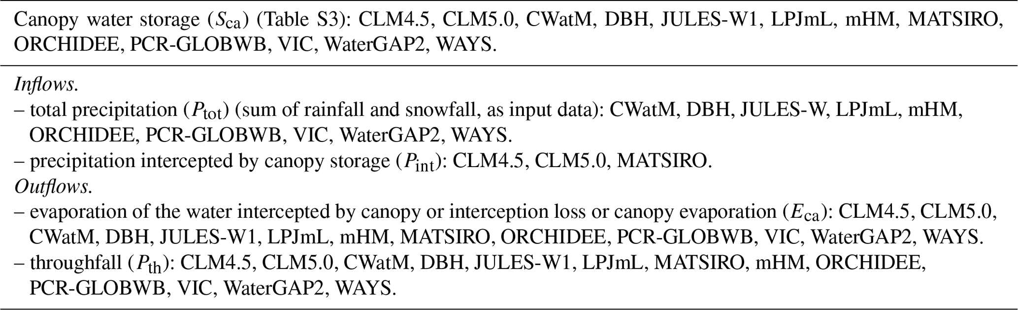
Table 2Snow and soil compartments and their water flows included in ISIMIP2b global water models.
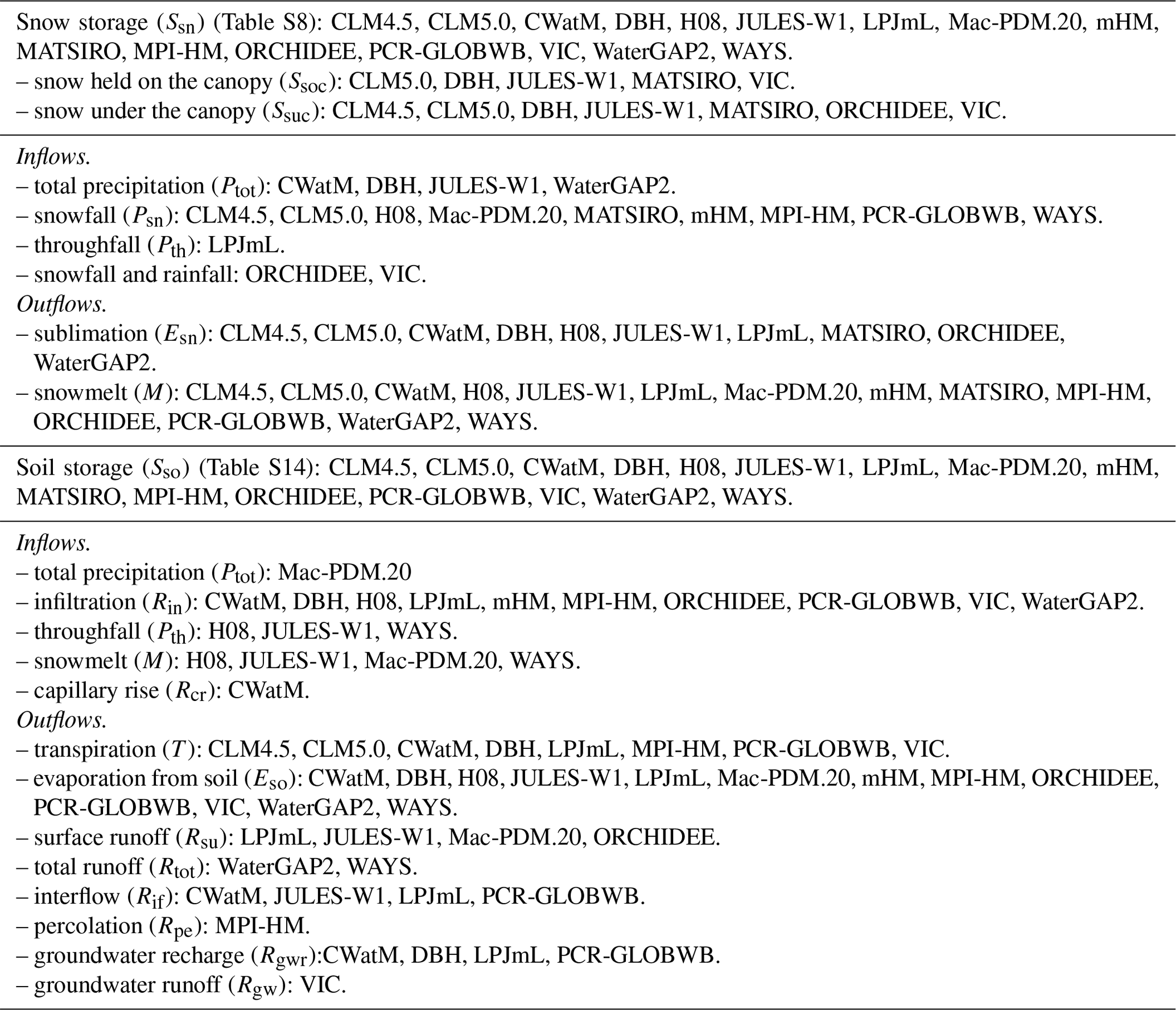
Table 3Groundwater, lake, reservoir, and wetland compartments and their water flows included in ISIMIP2b global water models.
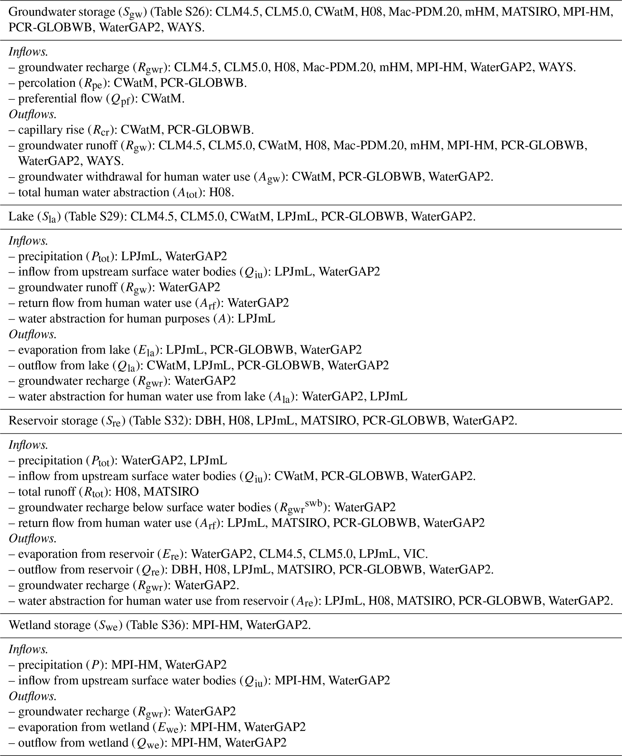
Table 4River compartment and its water flows included in the ISIMIP2b global water models.
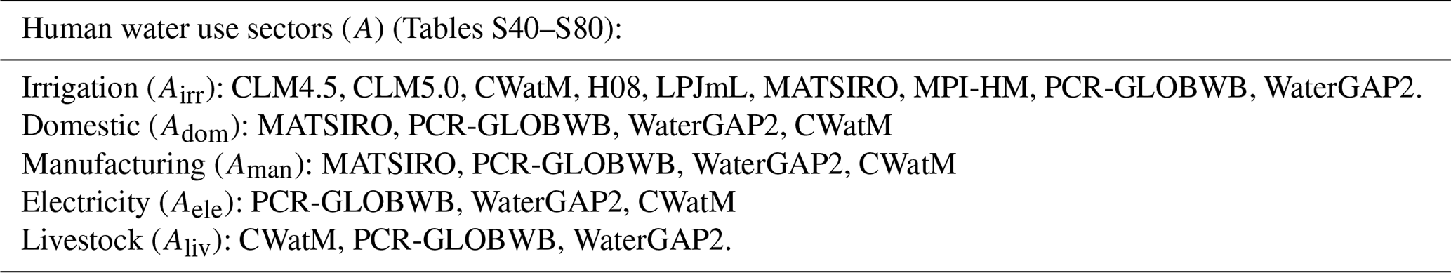
Table 6Key characteristics of the global water models.
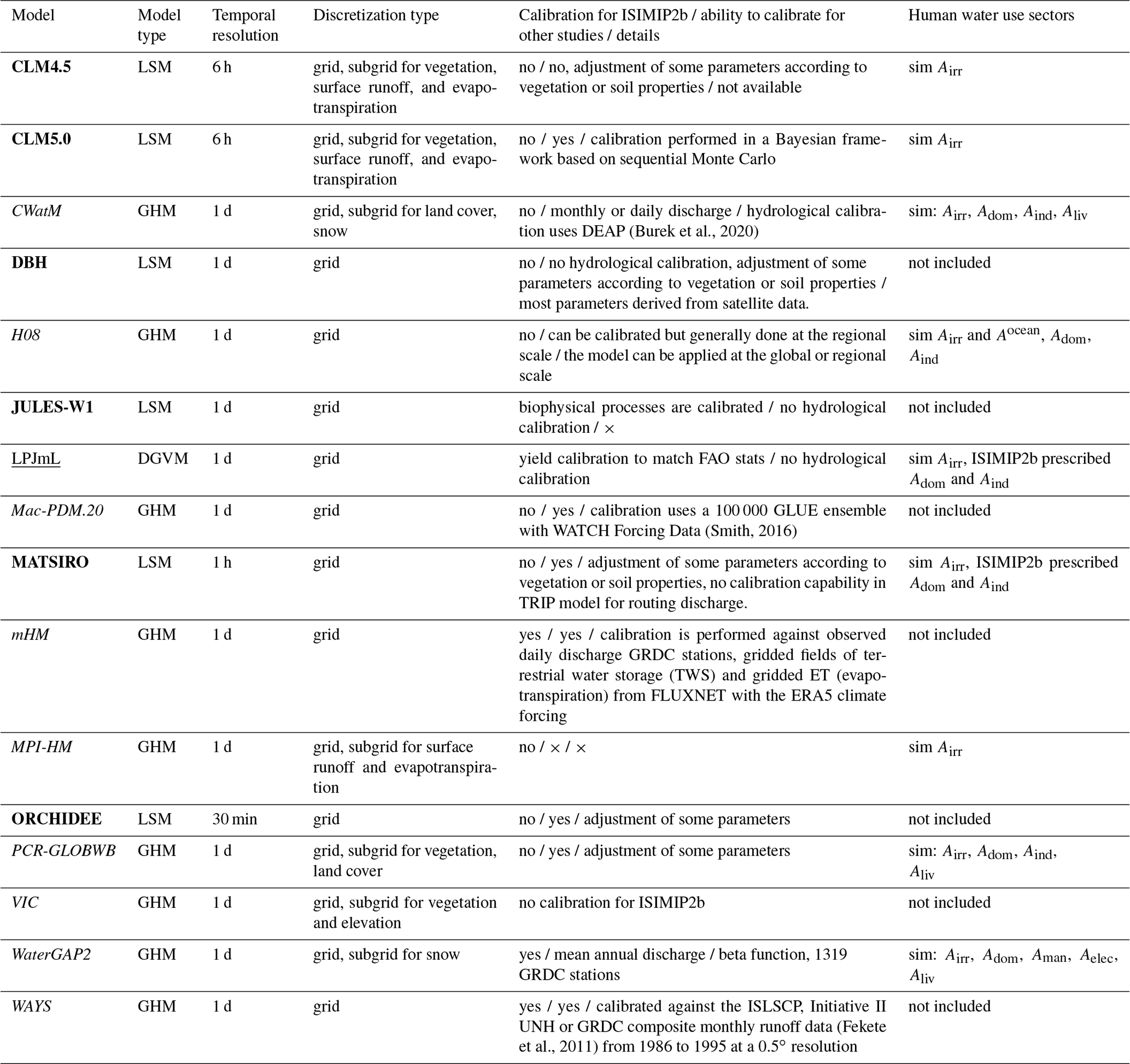
×: no details; DEAP: Distributed Evolutionary Algorithms in Python; DGVM: dynamic global vegetation model; EB: energy balance; GHM: global hydrological model; GRDC: Global Runoff Data Centre; ISLSCP: International Satellite Land Surface Climatology Project; LSM: land surface model; sim: simulated by the model; UNH: University of New Hampshire; Airr: water abstractions for irrigation; Adom: water abstractions for domestic; Aman: water abstractions for manufacturing; Aele: water abstractions for cooling of thermal power plants; Aind: water abstractions for industry (sum of Aman and Aele); Aliv: water abstractions for livestock; TRIP: Total Runoff Integrating Pathways. Bold font indicates LSMs, italic font indicates GHMs, and underlined font indicates DGVMs.
4.3 Creation of glossary with variable definitions
We decided upon clear definitions of the analysed variables. However, we encountered many ambiguities and challenges in defining the analysed variables and labelling processes as being similar or different among them. Some examples are presented in the following lines. We present other definitions of water storage compartments, flows, and human water use sectors used in this paper in the Supplement (Table S84).
We decided to use the expression “input data” for climate variables of the 16 GWMs to avoid confusion among readers. We define “parameterization” as changes of model parameter values (Samaniego et al., 2010).
We use “active vegetation” to highlight if models include the photosynthesis scheme in their structure and if they have the ability to simulate active changes in vegetation in an area because of changes in the CO2 concentration, air temperature, and precipitation. We use “dynamic vegetation” to define changes in vegetation from one geographical area to another because of competitive and biogeographical processes determined by climate change (geographical distribution of plants) or human activities. We decided to use “sub-surface runoff” synonymously with “interflow” and to define it as the amount of water that leaves the soil layer laterally.
We define “baseflow” as the low part of the streamflow that is supplied by groundwater, drainage from lakes, wetlands, glaciers, and interflow during long periods when no precipitation or snowmelt occurs. Ultimately, we have excluded the variable baseflow from the analysis because it is not simulated by 16 GWMs in ISIMIP2b.
We discovered that “groundwater runoff” and baseflow are used synonymously and define the water that leaves groundwater storage. We also found that baseflow and sub-surface runoff are used synonymously, and define the amount of water estimated for the third soil layer (VIC). We noticed that MPI-HM includes additional storage, called “baseflow storage”, that collects the drainage leaving through the bottom of the soil storage and applies a substantial time lag before passing it on to the river storage. In ISIMIP2b, the drainage computed by MPI-HM was submitted as sub-surface runoff, but considering that this baseflow storage acts similarly to a groundwater storage, drainage could be used as groundwater recharge in ISIMIP3a/b. Consequently, its outflow could be submitted as groundwater runoff. However, the purpose of this baseflow storage, for MPI-HM, is predominantly to cause a delay in river discharge and not to simulate groundwater in detail.
We decided to define “groundwater recharge” as the amount of water that reaches the groundwater storage, because of its hydrological meaning. However, we found out that the words “drainage” (MPI-HM), “aquifer recharge” (CLM4.5), and groundwater recharge (GHMs) are used synonymously among 16 GWMs. ISIMIP2b relates “seepage” with groundwater recharge for the models that do not include a groundwater storage, supposing that this water would reach groundwater storage if it would exist.
Another discovery was that “throughfall” and “drip” in some models were considered synonyms and that they were used to describe precipitation that falls to the ground through canopy spaces (CLM4.5, CLM5.0, MATSIRO). In this case, we decided to separate these words and to define throughfall as being precipitation that falls to the ground through canopy spaces and drip as being precipitation that leaks at the edge of canopy.
In this study, we define streamflow as the volumetric flow rate of water through a river cross section. Therefore, the streamflow is the water transfer that is routed through a channel towards the ocean or towards an inland sink. We define the total runoff as the (not routed) total amount of water that runs off the grid cell, either over the soil surface or from the sub-surface (lateral flow). In some studies, the streamflow is converted to runoff by dividing the streamflow values with the area upstream of the gauging station (for example, the area upstream of station according to the DDM30 river network; see Döll and Lehner, 2002).
In summary, in global water modelling, we need to be aware of differences in vocabulary. A widely accepted list of definitions would avoid confusion and facilitate successful interaction and collaboration. Furthermore, we need to clarify hydrological terms for peers from other disciplines, stakeholders, and a general audience (Brunner et al., 2018) to facilitate easier communication, understanding, and analysis.
4.4 Variable naming
We notated each variable of model equations. We used multiple subscripts and superscripts to properly identify water storage compartments, flows, and human water use sectors because of the large number of storage compartments included in the model structures. We selected “S” to describe water storage, “P” to describe everything connected to precipitation, “E” for everything related to evaporation, “R” for everything related to runoff, “Q” for everything related to streamflow and outflow, and “A” for water abstractions. We used two letters for subscripts and superscripts, ideally, the first two letters of the word, for example, “ca” for canopy, “sn” for snow, “so” for soil, and so on (see the list of symbols and glossary in the Supplement), while we used the first letter of each word in the case of compounds words such as groundwater (“gw”) or surface water (“sw”). We separated subscripts and superscripts from one another using comma. We did not write full words for subscripts and superscripts because equations became too long and difficult to read and understand. Some of these decisions correspond with some habits that exist in the hydrological community (e.g. gw and sw), and we decided to keep them to make a comfortable and easy workflow for modellers and readers.
4.5 Collection of the equations from the modelling teams
In the next step, modelling teams created and provided the model equations used to provide simulations for ISIMIP2b according to the generated lists. Each modelling team involved in this study internally checked and reviewed its model, based on the model code and peer-reviewed articles mentioned in Table 11 or only on the peer-reviewed articles on model description mentioned in Table 11. In some cases, modelling teams provided the equations using our standard writing style and symbols presented in Sect. 4.4, while in other cases they used their specific writing style. Therefore, the modelling teams checked the model equations on their correctness.
4.6 Homogenization of the model equations
We homogenized all variables and standardized variables' units in Tables S1–S83. We used the Overleaf platform, an online LaTeX editor, with its glossaries package, to homogenize all model equations of 16 GWMs, write some model equations, and rewrite other model equations using our symbols. This online LaTeX editor enabled online collaboration, correction of model equations many times, and saving a lot of time in all this process. Therefore, the Supplement provides an overview of the 16 GWMs, analysed in this study, and enables readers to understand similarities and differences among these models and identify included water compartments and human water use sectors and their flows. Ultimately, the readers get an overview of hydrological knowledge complexity behind these models (Tables S1–S97).
4.7 Evaluation of collected information
In the final step, we re-evaluated the collected and homogenized model equations for their consistency with the model code. We found similarities and differences among 16 GWMs analysed in this study. We analysed the model equations to find the models that simulate the same water flow (e.g. evaporation), the same water storage compartment (e.g. canopy storage), the same human water use sector (e.g. irrigation sector). For example, five models (CWatM, JULES-W1, MATSIRO, MPI-HM, and WAYS) use the same equation to compute potential evapotranspiration in Table S2. A total of 10 models (CWatM, DBH, JULES-W1, LPJmL, mHM, ORCHIDEE, PCR-GLOBWB, VIC, WaterGAP2, and WAYS) compute changes in canopy water storage taking into account the same variables such as total precipitation, throughfall, and canopy evaporation. The other three models (CLM4.5, CLM5.0, and MATSIRO) compute changes in canopy water storage differently than the nine models by taking into account the precipitation intercepted by canopy storage and liquid and solid throughfall, in addition to canopy evaporation (Table S3). We also conclude that 12 models compute canopy evaporation (Tables S3, S7). Therefore, in the next section (Sect. 5), we present our results according to two main parts of the terrestrial water cycle: the hydrological part and water use part. The hydrological part includes the eight water storage compartments and their flows, while the water use part includes five human water use sectors and their flows.
Several studies highlighted the need to understand better modelling approaches, model structures, model equations, and similarities and differences among models (Zhao et al., 2017; Veldkamp et al., 2018; Schewe et al., 2019). Therefore, in this section, we present some similarities and differences among 16 GWMs in simulating the terrestrial water cycle. This information enables us to interpret the different model results found in some model comparison and ensemble studies (Zaherpour et al., 2018; Wartenburger et al., 2018; Scanlon et al., 2019), as well as those by Gudmundsson et al. (2021), Reinecke et al. (2021), and Pokhrel et al. (2021). This information also strengthens our understanding of how these models work. Briefly, the 16 analysed GWMs include similar hydrological processes in their structure, but they have different model structures.
5.1 Similarities and differences in simulating eight water storage compartments
5.1.1 Canopy water storage
The changes in canopy water storage depend on how much water evaporates (canopy evaporation) and how much water is intercepted by canopy. Three models do not compute potential evapotranspiration (Tables S2, 7, and 8). Seven models apply the Penman–Monteith method to compute potential evapotranspiration (PET). PCR-GLOBWB applies the Hamon method to simulate PET, while mHM applies the Hargreaves–Samani method. ORCHIDEE applies a simplified Penman–Monteith equation (Monteith, 1965) with a correction term developed by Chris Milly (1992). WaterGAP2 and LPJmL apply the Priestley–Taylor equation, while H08 and MATSIRO apply the Bulk method.
A total of 13 models include canopy water storage in their structure, while 3 other models do not include it (H08, Mac-PDM.20, and MPI-HM: Table S3, Fig. 1). A total of 10 models compute canopy water storage by subtracting the throughfall amount and canopy evaporation from the total precipitation. The other 3 models (CLM4.5, CLM5.0, and MATSIRO) compute change in canopy water storage by subtracting the liquid or solid throughfall and canopy evaporation from the precipitation intercepted by the canopy storage. MATSIRO is the only model that has two canopy water compartments: one for rainfall interception and one for snowfall interception. It also computes in detail how much water is intercepted by canopies in stormy areas with high wind speeds and in calm areas with low wind speeds. In these areas, precipitation depends mainly on leaf area index (LAI) and water deficit in the canopy storage.
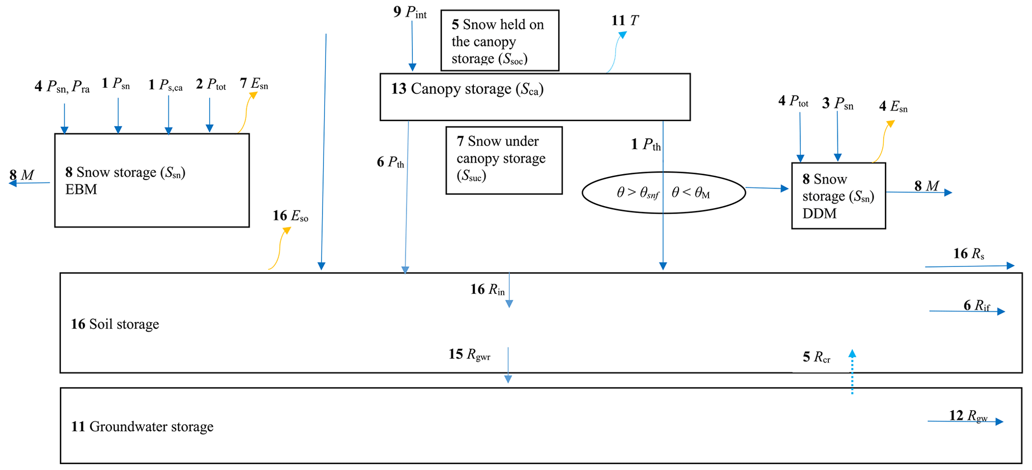
Figure 1Scheme with number of models that compute vertical water balance in ISIMIP2b. Abbreviations are as follows. DDM: degree-day method; EBM: energy balance method; Esn: sublimation; Eso: soil evaporation; M: snowmelt; Pgr: total precipitation falls directly to the ground; Pint: precipitation intercepted by canopy; Psn: snowfall; Pra: rainfall; Pth: throughfall; Ptot: total precipitation; Ps,ca: snowfall that is affected by the canopy interception and dripping; Rcr: capillary rise; Rgw: groundwater runoff; Rgwr: groundwater recharge; Rif: interflow; Rin: infiltration; Rs: surface runoff; T: transpiration; θ: air temperature;θsnf : snow freeze temperature; θM: melting temperature. Bold font indicates the number of models that compute water flows and water storage compartments in ISIMIP2b. Blue arrows show water flow, and orange arrows show evaporation.
Three land surface models (CLM4.5, CLM5.0, and MATSIRO) divide total precipitation into precipitation intercepted by canopy, precipitation that penetrates the canopy and then reaches the ground (throughfall), and precipitation that falls directly on the ground (Tables S4–S6). Therefore, these models distinguish between rainfall and snowfall. Further, they also divide throughfall into liquid and solid phases.
Two models compute an interception scheme based on a leaf and stem area index, while seven models use only a leaf area index (Tables 7 and 8). A total of 10 models compute this considering vegetation type (a plant functional type system) (Tables 7 and 8). MPI-HM uses prescribed data taken from Land Surface Parameter dataset version 2 (Hagemann, 2002). PCR-GLOBWB uses the HYDE3.2 (Klein Goldewijk, 2017), MIRCA (Portmann et al., 2010), and GlobCover datasets (Bicheron et al., 2011). Generally, prescribed vegetation ignores the decisive interaction between vegetation and runoff and interactions between the atmosphere and Earth's surface (Gerten et al., 2004; McPherson, 2007; Nicholson, 2000). In the ISIMIP2b, the word “prescribed” has two meanings: (i) data which are simulated by other models and provided by the ISIMIP2b framework as input (for example, https://www.isimip.org/gettingstarted/details/38/, last access: 8 June 2021) and (ii) data obtained from satellite observations, other datasets, or maps. Prescribed data highlight some limitations of the models or underline the lack of some processes that were intentionally or unintentionally removed from the model structure, according to the purpose of the model development or other priorities such as time.
Table 7Representation of the water storage compartments and water flows included in the global water models (part i).
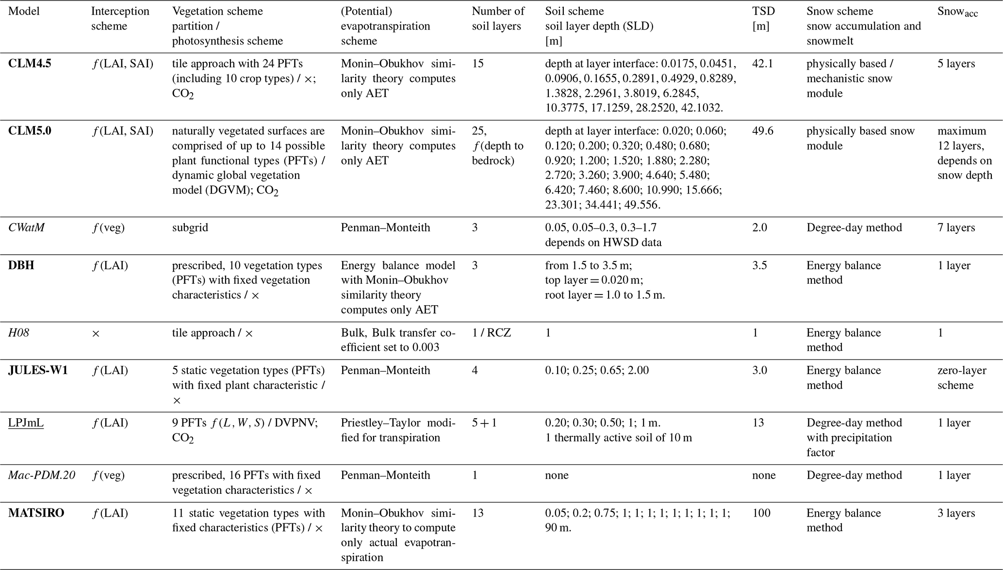
AET: actual evapotranspiration; CO2: CO2 fertilization effect; DGVM: dynamic global vegetation model; DVPNV: dynamic vegetation composition on potential natural vegetation areas; f(LAI): function of leaf area index; f(LAI,SAI): function of leaf area index (LAI) and stem area index (SAI); f(veg): function of vegetation type; HWSD: Harmonized World Soil Database (FAO/IIASA/ISRIC/ISSCAS/JRC (2012): Harmonized World Soil Database (version 1.2), FAO, Rome, Italy and IIASA, Laxenburg, Austria, available at: http://www.fao.org/soils-portal/soil-survey/soil-maps-and-databases/harmonized-world-soil-database-v12/en/, last access: 10 June 2021); L: light; PFTs: plant functional types; RCZ: runoff properties varies with climate zones; SLD: soil layers depth from top to bottom; TSD: total soil layer depth; Snowacc: snow accumulation; S: space; W: water; ×: not included in the model. Bold font indicates LSMs, italic font indicates GHMs, and underlined font indicates DGVMs.
Table 8Representation of the water storages compartments and water flows included in the global water models (part ii).
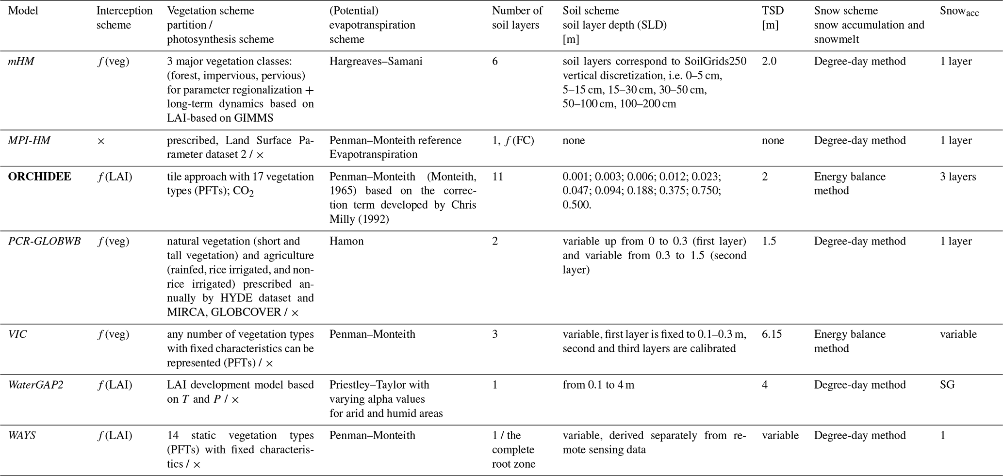
AET: actual evapotranspiration; CO2: CO2 fertilization effect; f(LAI): function of leaf area index; f(veg): function of vegetation type; f(FC): function of field capacity; P: precipitation; PFTs: plant functional types; SG: subgrid; SLD: soil layers depth from top to bottom; TSD: total soil layer depth; Snowacc: snow accumulation; T: subgrid temperature (daily average) (0 ∘C); ×: not included in the model. Bold indicates LSMs, and italic indicates GHMs.
Throughfall is estimated by 13 models (Table S5) depending on (1) total precipitation and relative canopy water content (JULES-W1); (2) difference between total precipitation and canopy storage deficit (mHM, WaterGAP2, WAYS); (3) ratio between rainfall or snowfall and total precipitation (CLM4.5, CLM5.0, MATSIRO); (4) total precipitation and minimum value of potential evapotranspiration (PET) or canopy storage (LPJmL); (5) canopy water content (PCR-GLOBWB); (6) a function of LAI then weighted by the canopy fraction in the grid cell (DBH and ORCHIDEE); (7) canopy water content and grid cell average precipitation (VIC); and (8) total precipitation, canopy water content, and canopy evaporation (CWatM). Three models (H08, Mac-PDM.20, MPI-HM) do not estimate throughfall.
Four models (CLM4.5, CLM5.0, LPJmL, and ORCHIDEE; Tables 7 and 8) account for the CO2 fertilization effect, in the LAI estimation, by using a photosynthesis scheme (active vegetation, mentioned in Sect. 4.3), and they have the ability to simulate the CO2 effect on plant functioning. Sitch et al. (2008) found that simulations on CO2 fertilization effect depend on the number of plant functional types (PFTs) prescribed or defined in the model and on the processes used to estimate plants' ability to adapt, acclimate, and grow in new environmental conditions.
5.1.2 Snow water storage
Snow storage accumulates snow below freezing temperatures and declines by melting and surface and/or snowdrift sublimation. GHMs typically use the degree-day method to compute snow accumulation and snowmelt, while LSMs use the energy balance method (Tables 7 and 8, Fig. 1). Among GHMs, H08 is the only one that applies the energy balance method to compute snow accumulation and melt. Additionally, three models (CLM4.5, CLM5.0, and CWatM) include glacier storage. CLM4.5 and CLM5.0 use a mechanistic snow module to calculate snow accumulation and melt; therefore, they include multiple snow layers where compaction, melt, refreezing, firn, and other snow-related processes take place.
Four models (CLM4.5, CLM5.0, MPI-HM, and VIC) have two water storage compartments for snow: for estimation of frozen water and for liquid water content (Table S8). WaterGAP2 calculates snow accumulation and melting in 100 subgrid cells (Schulze and Döll, 2004; Müller Schmied et al., 2014), while CWatM calculated using 3 to 10 elevation zones per grid. Five models (CLM5.0, DBH, JULES-W1, MATSIRO, and VIC) estimate snow held on the canopy (Table S9). Further, seven models differentially estimate snow under the canopy (Table S10). Five models do not estimate sublimation: Mac-PDM.20, mHM, MPI-HM, PCR-GLOBWB, and WAYS (Table S11). All models simulate snowmelt (Table S12). MATSIRO is the only model that distinguishes between sublimation and evaporation on snow-covered ground and snow-free ground. The number of snow layers is fixed, and it varies among 16 GWMs between 1 (most of the GHMs) and 12 (CLM5.0; Tables 7 and 8). Most of the GWMs present no upper limit for snow storage (Tables S48–S51).
5.1.3 Soil water storage
Soil water storage keeps and loses water from flows above and below the ground's surface. Hydrologically, this includes the unsaturated zone or vadose zone, the part of Earth between the land surface and the top of the phreatic zone (water table).
Soil hydrologic processes
Overall, 10 models consider initial infiltration as inflow of the soil storage, while 3 models (H08, JULES-W1, and WAYS) consider throughfall (Table S14). Mac-PDM.20 considers total precipitation as inflow of soil storage (Table S14). Thus, infiltration, throughfall, and total precipitation have different values among 16 models because the models compute infiltration and throughfall differently, while total precipitation represents the input data for some models. All models compute surface runoff (Table S20, Fig. 1), soil evaporation (Table S24), and infiltration (Table S25), while six models compute interflow (Table S26). H08 computes runoff properties varying according to the climate zone (Table 7).
CLM4.5 includes an empirical soil evaporation resistance method, while CLM5.0 includes a mechanistically based method where the soil evaporation is controlled by a dry surface layer. Therefore, CLM5.0 has the ability to model the seasonality of soil evaporation and soil water storage in (semi)arid regions. It also explicitly simulates spatial variation in soil thickness (0.4 to 8.5 m) and columnar water holding capacity, unlike CLM4.5 (Lawrence et al., 2019). These models have a large number of soil layers, each having moisture storage potential depending on the soil texture. They use the same approach to calculate surface runoff and have the ability to compute liquid runoff and solid runoff from snow capping. Both models consider sub-surface runoff as a product of an exponential function of the water table depth and a single coefficient (Niu et al., 2005). VIC uses the variable infiltration curve (Zhao et al., 1980) to account for the spatial heterogeneity of runoff generation and assumes that surface runoff from the upper two soil layers is generated by those areas where precipitation exceeds the storage capacity of the soil. The mHM model has one more bucket between the soil storage and groundwater storage, named “unsaturated storage”, representing the source for interflow and groundwater recharge.
LPJmL was adjusted, and the water from the uppermost soil layers is considered to contribute to surface runoff if an excess of storage is calculated according to the infiltration or percolation rates, which depend on soil type. LPJmL routes what was previously lateral runoff from “layer 0” (first 20 cm) as surface runoff.
In JULES-W1, water that reaches the soil surface is split between water that infiltrates into the soil and surface runoff. Infiltration takes place at a rate equal to saturated hydraulic conductivity multiplied by an infiltration enhancement factor, which is dependent on the presence and type of vegetation. If a soil layer becomes saturated, the water in excess of saturation is put into the layer below. JULES-W1 also uses a “zero-layer” scheme that does not use explicit model layers to represent snow, instead adapting the topsoil level to represent existent snow processes. In the original zero-layer, the snow scheme has a constant thermal conductivity and density. Bulk thermal conductivity of snow on the surface layer decreases due to both the increased layer thickness and the different conductivities of snow and soil. Surface energy balance and heat flux between the surface layer are controlled by insulation factors and layer thickness (Best et al., 2011). WAYS simulates the water storage and flows in soil only for the entire root zone (Table 8). In the DBH model, runoff is generated directly when soil layer is saturated or is generated when rainfall intensity is larger than the infiltration rate estimated with the Green–Ampt method (Tang et al., 2006).
Two models (CWatM and MPI-HM) have an additional water storage compartment to compute the runoff concentration in a grid cell that has a lag time before entering the river storage compartment (Table S44). Consequently, this storage serves to create a delay between runoff and streamflow and accounts for the average distance that runoff, generated at a specific point within a grid cell, has to travel before reaching the river. This storage collects water from rivulets and creeks or concentrates runoff in rivulets and creeks before it enters the river storage because the rivulets and creeks are smaller than the size of a single grid cell and have different water retention properties from the main river channel within the grid cell. Therefore, this compartment does not act as a floodplain to delay floods or as overland flow to express too much water in the soil. In its original structure, MPI-HM named this compartment “overland flow”, but we decided to rename it “rivulet storage” to avoid confusion among readers.
Some GWMs compute vertical water movement in unsaturated soils by applying the Richards equation (Richards, 1931; e.g. CLM4.5, CLM5.0, CWatM, JULES-W1, MATSIRO, ORCHIDEE, VIC). However, the Richards equation may not be relevant for the models that have one soil layer because of its complexity and of missing capillary rise (Lee and Abriola, 1999; Farthing and Ogden, 2017). LPJmL uses a percolation scheme to estimate vertical water movement that applies the storage routine technique developed by Krysanova et al. (2000) and simulates free water in the soil bucket. DBH uses the Green–Ampt equation to compute infiltration in unsaturated soils.
Five models compute capillary rise (CLM4.5, CLM5.0, CWatM, MATSIRO, and PCR-GLOBWB), with CWatM and PCR-GLOBWB using the same approach (Table S28).
Soil column configuration
The number of soil layers ranges between 1 (H08, MPI-HM, and WaterGAP2) and 25 (20 soil layers + 5 bedrock layers: CLM5.0), while total soil depth varies between 1 m (H08) and 49.6 m (CLM5.0; Tables 7 and 8). ORCHIDEE uses a relatively deep soil column to account for soil thermal processes. LPJmL has five hydrologically active soil layers plus one thermally active soil layer. MPI-HM defines soil storage in terms of the maximum water column, varying between 0 and 5 m; therefore, this cannot be translated into soil depth directly.
5.1.4 Groundwater storage
Groundwater storage, beneath the soil water storage compartment, receives water from drainage (e.g. MPI-HM), aquifer recharge (e.g. CLM4.5), or groundwater recharge (e.g. WaterGAP2) (Tables 9 and 10). It loses water through capillary rise, groundwater runoff, and groundwater abstraction for human water use. In GWMs, the groundwater compartment hydrologically simulates the saturated zone or phreatic zone (WaterGAP2) or an unconfined aquifer (CLM4.5). A total of 11 models include groundwater storage in their structure, and most of them have only one groundwater layer (Table S29, Fig. 1). In ISIMIP2b, two models (JULES-W1 and LPJmL) consider the water excess from the bottom soil layer as seepage and equate this variable with groundwater recharge because they do not have a groundwater compartment.
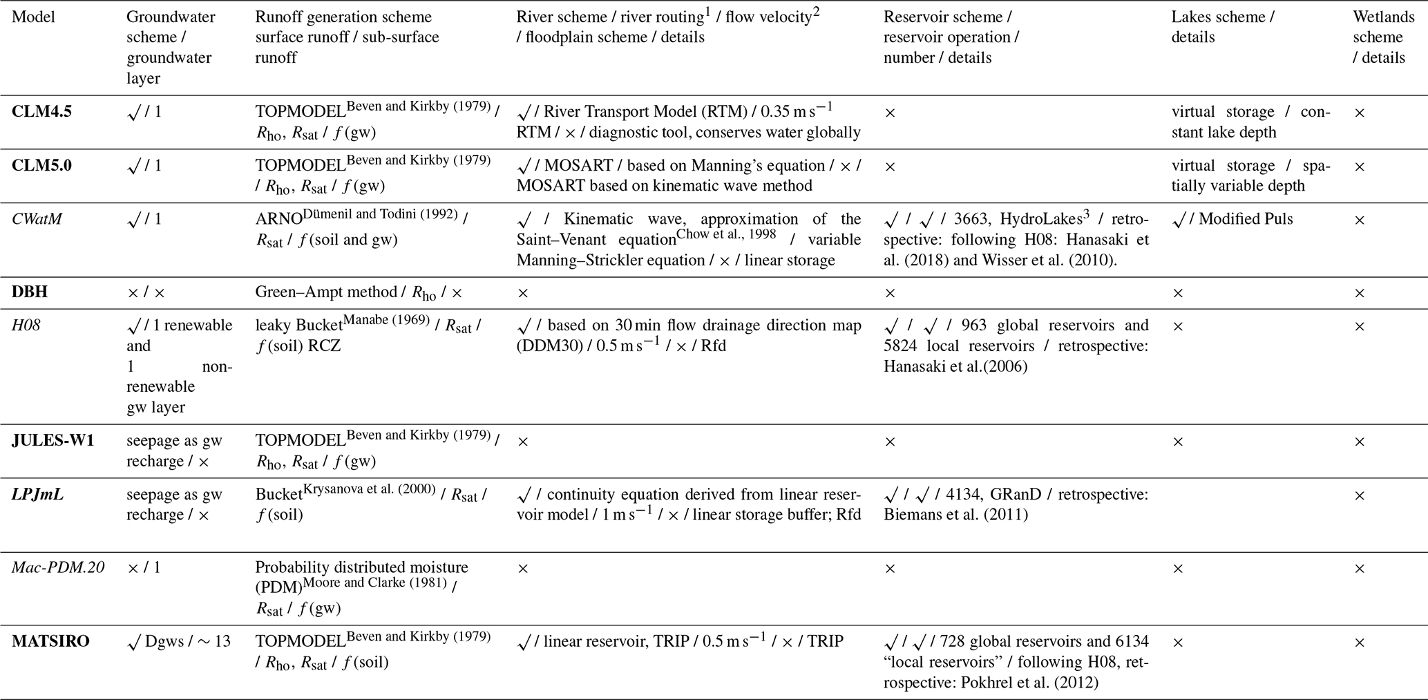
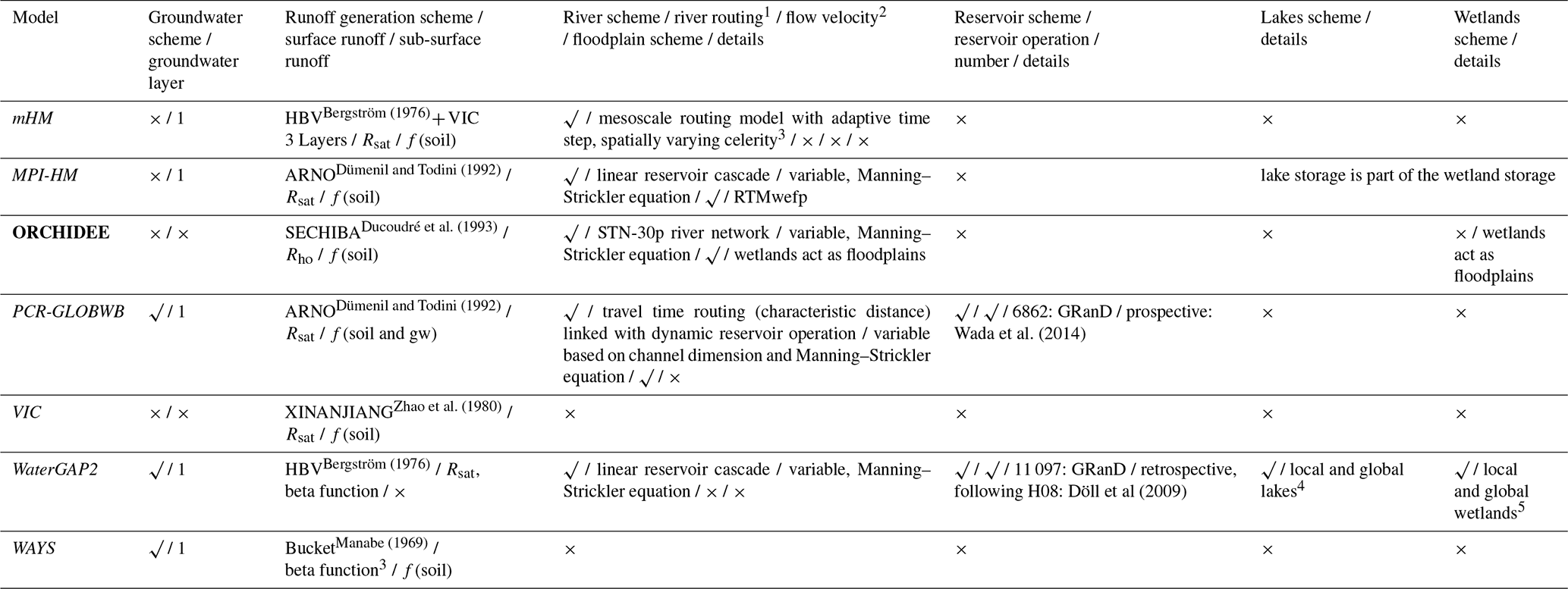
Table 9Representation of the water storage compartments and water fluxes included in the global water models (part iii).
√: included in the model; ×: not
included in the model for ISIMIP2b simulations; Dgws: dynamic groundwater
scheme; GRanD: Global Reservoir and Dam database, according to Lehner et
al. (2011); gw: groundwater; Rsu: surface runoff; Rsat: Rsu modelled as saturation excess overland flow; Rho: Rsu modelled as infiltration excess or Hortonian overland flow; f(gw): sub-surface flow or interflow modelled as a function of groundwater;
f(soil): sub-surface flow or interflow modelled as a function of soil
moisture (soil); Rfd: the model routes runoff along flow
direction; RTM: River Transport Model; TRIP: Total Runoff Integrating
Pathways. Bold font indicates LSMs, italic font indicates GHMs, and bold-italic font indicates DGVMs.
Notes: 1 data source: http://www.isimip.org (last access: 2 November 2020).
2 Zhao et al. (2017). 3 CWatM, HydroLakes
database: Messager et al. (2016); Lehner et al. (2011).
Table 10Representation of the water storage compartments and water fluxes included in the global water models (part iv).
√: included in the model; ×: not
included in the model for ISIMIP2b simulations; GRanD: Global Reservoir
and Dam database according to Lehner et al. (2011); gw: groundwater;
Rsu: surface runoff; Rsat: Rsu modelled as saturation
excess overland flow; Rho: Rsu modelled as infiltration
excess or Hortonian overland flow; f(gw): sub-surface flow or interflow
modelled as a function of groundwater; f(soil): sub-surface flow or
interflow modelled as a function of soil moisture (soil); RTMwefp: routing model with wetlands (we) and floodplain (fp) scheme.
Bold font indicates LSMs, and italic font indicates GHMs.
Notes: 1 Data source: http://www.isimip.org (last access: 2 November 2020).
2 Zhao et al. (2017). 3 Thober et al. (2019); 4
and 5 WaterGAP2, Döll et al. (2012).
CLM4.5 simulates an unconfined aquifer as a groundwater component below the saturated soil storage and with a prescribed maximum value (5000 mm), while CLM5.0 simulates an impermeable bedrock with five layers and therefore assumes no groundwater flow as bottom boundary conditions. In CLM4.5, the unconfined aquifer interacts with the saturated soil storage through the water table, whether it is within or below this storage. When the water table is below the soil storage, the aquifer recharge is estimated by applying Darcy's law across the water table (Lawrence et al., 2019).
MATSIRO has a dynamic groundwater scheme (Koirala et al., 2014; Pokhrel et al., 2015) in which the number of soil layers in the saturated zone (i.e. groundwater) varies in time between 1 and 13 depending on the water table location (Table 7). The two-way interaction between the unsaturated zone (for which vertical moisture movement is resolved by solving the Richards equation) and the underlying aquifer is simulated through moisture flux exchange at the water table. This flux exchange is determined as the algebraic sum of downward gravity drainage from the unsaturated soil layer overlying the water table and the upward capillary flux (Koirala et al., 2014; Pokhrel et al., 2015). The water balance of the saturated zone is resolved by considering recharge to the groundwater aquifer and groundwater runoff that is determined by using a two-parameter, statistical dynamical formulation considering soil hydraulic properties and basin geomorphology (Yeh and Eltahir, 2005). The variation in the water table is also determined by the aquifer-specific yield.
In Mac-PDM.20, it is assumed that all water in excess of field capacity drains in 1 d to the deep store, which for ISIMIP2b is used to represent groundwater recharge (Rgwr). The total runoff (qtot) is the sum of direct runoff (qs) plus delayed runoff from the deep soil and groundwater (qsb). This delayed runoff (qsb) is assumed to be a non-linear function of the amount of water held in the groundwater and deep soil store (Table S31). Thus, like with MPI-HM, the purpose of the delayed runoff (or baseflow) is predominantly to cause a delay in river discharge and not to simulate groundwater in detail.
H08 separates groundwater into renewable and non-renewable layers (Hanasaki et al., 2008). WaterGAP2 is the only model that simulates the groundwater recharge from surface water bodies in semiarid and arid grid cells (Döll et al., 2014).
A total of 15 models compute groundwater recharge, with 3 using the same approach (H08, WaterGAP2, and WAYS: Döll and Fiedler, 2008; Table S30), while 12 models compute groundwater runoff (Table S31).
5.1.5 Lake storage
Lake storage fills with water through flows above and below the ground and stores water for a certain residence time. It loses water through discharge to other storage compartments, evaporation, groundwater recharge, and water abstraction for human water use. A total of 10 models do not include lakes (Tables 9 and 10; Fig. 2). Five models compute evaporation from lakes, three of them based on a PET approach (Table S33), while four models compute outflow from lakes (Table S34). CLM4.5 and CLM5.0 compute the lake storage as virtual storage where the difference between precipitation and evaporation is balanced automatically by their outflow, named “lake runoff”. CLM4.5 uses constant lake depth, while CLM5.0 uses spatially variable lake depth, and freezing and thawing are included in the lake body (Vanderkelen et al., 2020).
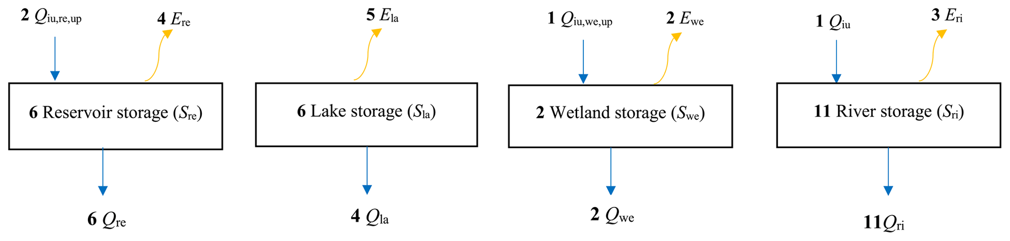
Figure 2Number of global water models that compute lateral water balance in ISIMIP2b. Ela: evaporation from lake; Ere: evaporation from reservoir; Eri: evaporation from river; Ewe: evaporation from wetland; : inflow from upstream cell for reservoir storage; : inflow from upstream cell for wetland storage; Qla: outflow from lake; Qre: outflow from reservoir; Qri: streamflow, Qwe: outflow from wetland. Bold font indicates the number of models that compute lateral water balance in ISIMIP2b. Blue arrows show water flow, and orange arrows show evaporation.
LPJmL treats natural lakes and rivers in a similar way in terms of inputs and output. Lake inputs to a river can also include upstream river inputs to the lake. LPJmL also keeps track of a lake fraction in the river input. WaterGAP2 and CWatM have two types of lake storage: “local lake storage” gets water from runoff resulting within the cell, and “global lake storage” gets water from runoff resulting within the cell and the upstream cell (Müller Schmied et al., 2021).
5.1.6 Reservoir storage
Reservoir storage fills with water behind dams through flows above and below the ground and stores water for a residence time. It loses water through discharge to other storage compartments, evaporation, groundwater recharge, and water abstraction for human water use. A total of 10 models (CLM4.5, CLM5.0, DBH, JULES-W1, Mac-PDM.20, mHM, MPI-HM, ORCHIDEE, VIC, and WAYS) do not include reservoir storage for ISIMIP2b (Tables 9, 10, S35; Fig. 2). Six models compute outflow from reservoirs (Table S37), while evaporation from reservoirs is computed by four models (Table S38).
In general, most of the models use the Global Reservoir and Dam database (GRanD: Lehner et al., 2011) but with a different number of active managed reservoirs used for reservoir operation during simulations. Three models (LPJmL, WaterGAP2 and PCR-GLOBWB) merge more than one reservoir per grid cell into one reservoir if required.
Four models (CWatM, H08, MATSIRO, and WaterGAP2) use two water compartments, global and local reservoirs, to represent the reservoirs, following the reservoir algorithm developed by H08. However, there are some differences in how the scheme was implemented in the models, mainly because of model structure, but the approach is essentially the same. These four models use the same approach in selecting active managed reservoirs for reservoir operation, but they use different thresholds. WaterGAP2 considers 1109 active managed reservoirs and handles reservoirs below 0.5 km3 storage capacity as local lakes. MATSIRO considers only 728 out of 6862 reservoirs for reservoir operation. In MATSIRO, global reservoirs have more than 1 km3 total storage capacity and “local reservoirs” or “ponds” have less than 1 km3 (around 6134 reservoirs; Hanasaki et al., 2006; Pokhrel et al., 2012). H08 considers 963 active managed reservoirs (global reservoirs) and 5824 local reservoirs; therefore, global reservoirs regulate river flow, while local reservoirs do not. Global reservoirs have 4773 km3 of total storage capacity, while local reservoirs have 1300 km3 of total storage capacity. In H08, when multiple local reservoirs are present in a grid cell, their capacity is added together. CWatM considers 3663 active managed reservoirs, while PCR-GLOBWB considers 6177. LPJmL includes 4134 reservoirs that become active after the first year of operation. In LPJmL, reservoirs are not managed according to an operation scheme, they are modelled as lakes with a maximum storage amount and the water over this amount is released as reservoir outflow; irrigation water can also be taken from the reservoir.
Five models (CWatM, H08, LPJmL, MATSIRO, and WaterGAP2) use a retrospective reservoir algorithm, while one model (PCR-GLOBWB) uses a prospective reservoir algorithm. The retrospective reservoir algorithm uses river flows and water demand, which were processed in a previous step, while the prospective reservoir algorithm uses forecasts of river flows and water demand (van Beek et al., 2011).
5.1.7 Wetland storage
Wetland storage fills and empties with water similarly to lake and reservoir compartments, except that water use is not satisfied from wetlands. Two models (MPI-HM and WaterGAP2) compute wetland compartment, evaporation, and outflow from land (Tables S39–S42; Fig. 2). WaterGAP2 has two types of wetland storage: “local wetland storage”, which obtains water from runoff resulting within the cell, and “global wetland storage”, which obtains water from runoff resulting within the cell and the upstream cell (Döll et al., 2012).
5.1.8 River storage
River storage is increased by surface and sub-surface runoff. It loses water through streamflow, evaporation, channel transmission, and water abstraction for human water use. Five models (DBH, JULES-W1, Mac-PDM2.0, VIC, WAYS) do not include river storage for ISIMIP2b simulations because of computational and resource constraints nor do they compute streamflow (Tables 9, 10, S43, and S46; Fig. 2). Four models (LPJmL, MATSIRO, MPI-HM, WaterGAP2) use a linear reservoir cascade approach to compute the water balance of the river storage (Tables 9 and 10). Furthermore, MATSIRO uses Total Runoff Integrating Pathways (TRIP) for river routing through a channel. Three models (CWatM, H08, and LPJmL) consider the minimum release for environmental flow. CWatM adopts a kinematic wave approach, approximation of the Saint–Venant equation (Chow et al., 1998), linked with dynamic reservoir and lake operation. Further, CWatM computes runoff concentrated in creeks and rivulets, with a lag time before entering the river storage, by using a triangular weighting function (Burek et al., 2020). ORCHIDEE includes a river transport module that involves the Simulated Topological Network (STN-30p). PCR-GLOBWB uses travel time routing (characteristic distance) linked with dynamic reservoir operation. For runoff and streamflow simulation, CLM4.5 uses a river transport model (RTM), while CLM5.0 uses a new mechanistic model for streamflow routing, called the Model for Scale Adaptive River Transport (MOSART; Oleson et al., 2013; Lawrence et al., 2019). The mHM model uses a mesoscale routing model with an adaptive time step according to the spatially varying celerity (Thober et al., 2019). Only MPI-HM and ORCHIDEE include a routing model with a wetlands and floodplain scheme, in which wetlands act as floodplains. Furthermore, ORCHIDEE includes swamps.
Six models (CLM5.0, CWatM, MPI-HM, ORCHIDEE, PCR-GLOBWB, WaterGAP2) apply the Manning–Strickler equation to estimate river flow velocity and use various values for it. CLM4.5 uses a standard river flow velocity of 0.35 m s−1, while H08 and MATSIRO use 0.5 m s−1 (Tables 9 and 10). LPJmL considers a standard river flow velocity of 1 m s−1. MPI-HM uses the Manning–Strickler equation only for flow velocity computation in wetlands, while for rivers it computes a slope-dependent flow velocity following the approach by Sausen et al. (1994).
Inflow from upstream grid cell surface water bodies represents the sum of inflow water from neighbouring upstream grid cells for CLM4.5, CLM5.0, CWatM, mHM, and WaterGAP2 (Table S45). Additionally, CWatM and WaterGAP2 also route this water through lakes and reservoirs before it reaches its final point. H08 computes it as being the product between a 0.5 m s−1 flow velocity and river storage from upstream grid cells. LPJmL considers it as being the outflow of river storage reduced by evaporation from lakes and reservoirs, while MPI-HM considers it as being the sum of outflow from rivulet storage, groundwater runoff, and streamflow from the upstream grid cells, then reduced by inflow from the wetland of an upstream grid cell. MATSIRO considers it as being the sum of inflow water from the neighbouring upstream grid cell multiplied by outflow of river from an upstream grid cell. ORCHIDEE calculates it as being the sum of stream river storage of upstream grid cells divided by topographic index of the retention time and a reduction factor of stream river storage. PCR-GLOBWB takes into account the outflow from river storage, time of process duration, length of river sections, and the coefficient friction of the reservoir weir.
Evaporation from rivers is computed only by three models, CWatM, LPJmL, and PCR-GLOBWB, based on a PET approach (Table S47).
5.2 Similarities and differences in simulating human water use sectors
Some GWMs simulate water extracted from surface water compartments and/or a groundwater compartment that is used for human activities. Human water abstraction represents the sum of the water consumed by humans, evaporative water and other water losses (named water consumption), and water returned to the groundwater or surface water compartments (named return flow, being the part of the water not consumed). Generally, three models extract water for human activities from groundwater or surface water bodies (H08, PCR-GLOBWB, and WaterGAP2). Seven models (DBH, JULES-W1, Mac-PDM.20, mHM, ORCHIDEE, VIC, and WAYS) do not include any human water use sectors in their structures (Table 6).
5.2.1 Irrigation sector
Irrigation water demand (potential irrigation water abstraction) is computed by nine models (Table S52). Groundwater abstraction for the irrigation sector is simulated by six models (CWatM, H08, MATSIRO, MPI-HM, PCR-GLOBWB, and WaterGAP2: Tables S53), while five models compute the return flow (Table S55). Irrigation surface water abstraction is calculated by nine models (Tables S56, S93–S94). CWatM includes a “normal irrigation scheme”, to mimic rainfall when the plants need it, and a paddy rice irrigation scheme, to mimic the flooding of the rice area (Table S56).
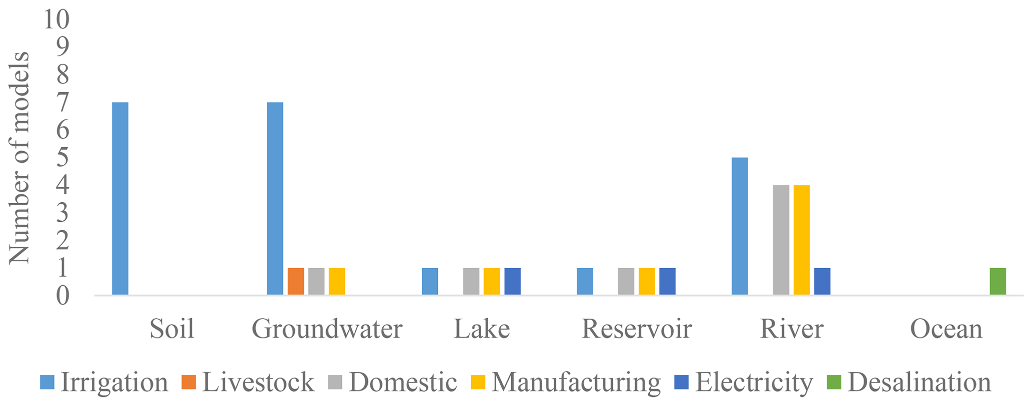
The water source for the irrigation sector is river for nine models (CLM4.5, CLM5.0, CWatM, H08, LPJmL, MATSIRO, MPI-HM, PCR-GLOBWB, WaterGAP2: Table S93). Six models (CWatM, H08, MATSIRO, MPI-HM, PCR-GLOBWB, WaterGAP2) consider groundwater a source for the irrigation sector (Table S93). Four models take water from lakes for the irrigation sector and five models take water from reservoirs (Fig. 3). Return flows from irrigation sector recharge mainly the soil and groundwater (seven models), while the return flows from domestic and manufacturing recharge mainly rivers (four models; Fig. 4).
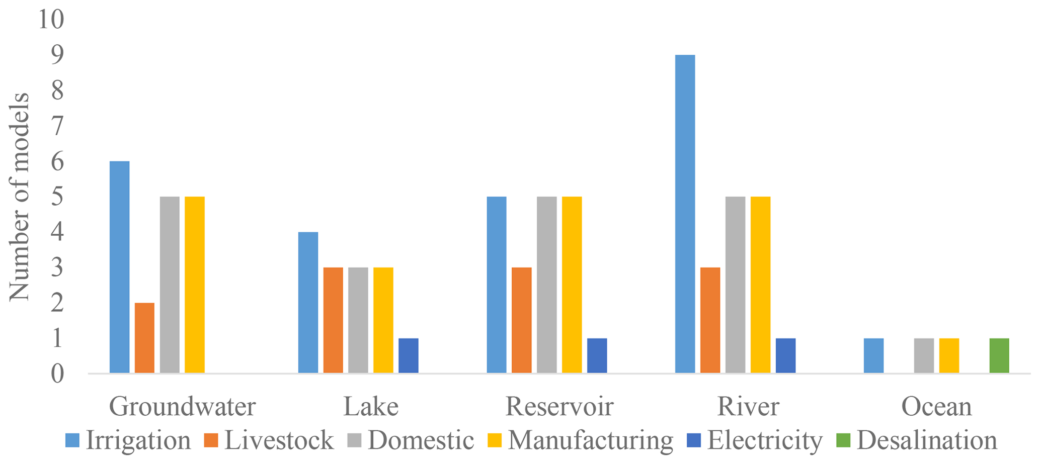
Figure 3Number of global water models that consider water source for human water use sectors in ISIMIP2b.
5.2.2 Domestic, livestock, and industry sectors
Five models (CWatM, H08, MATSIRO, PCR-GLOBWB, and WaterGAP2) simulate water abstraction, water consumption, and return flow for the domestic sector (household; see Tables S59–S64). Three models (MATSIRO, PCR-GLOBWB, and CWatM) combine manufacturing and electricity sectors into one sector, the industry sector. CWatM only calculates total abstraction from groundwater or surface water. MATSIRO and LPJmL used input data for water demand of the domestic and industry sectors, offered by the ISIMIP2b framework. These input datasets provide water consumption, but not return flow from these sectors. Consumption water can return to the atmosphere as evapotranspiration. LPJmL used input data for domestic and industrial water consumption data, provided by the ISIMIP2b framework, and assumed that only the consumed water amount is withdrawn. MATSIRO used input data for domestic and industrial water demand, and it computed the water abstraction and consumption itself for these sectors. ISIMIP2b does not offer input data for the livestock sector as the global numbers are low compared to other sectors (Müller Schmied et al., 2016). PCR-GLOBWB computes the amount of water abstracted and consumed for the livestock sector, taken from groundwater and surface water bodies (Tables S65–S68), while WaterGAP2 computes only the amount of water taken from surface water bodies for livestock (Tables S67–S68).
5.2.3 Surface water abstractions
Four models (CWatM, MATSIRO, MPI-HM, and WaterGAP2) compute total groundwater abstraction (Table S77). Five models (CWatM, LPJmL, MPI-HM, PCR-GLOBWB, and WaterGAP2) compute total lake abstraction (Table S78). Six models (CWatM, H08, LPJmL, MATSIRO, PCR-GLOBWB, and WaterGAP2) compute total reservoir abstraction (Table S79). Three models (CWatM, CLM5.0, and WaterGAP2) compute total river abstraction (Table S80).
CWatM sums up the water withdrawal from all users and distributes the total withdrawal to three different sources: (i) surface water, (ii) sustainable groundwater (renewable groundwater is the same as long-term groundwater recharge of the last 30 years in the analysed time interval), and (iii) unsustainable groundwater (non-renewable groundwater is the same as additional water gained by groundwater abstraction in surplus of groundwater recharge; Wada et al., 2012). Each withdrawal that is depleting the groundwater storage beyond groundwater recharge is using fossil groundwater (unsustainable groundwater).
MATSIRO and WaterGAP2 take similar approaches to compute groundwater abstraction: groundwater abstraction for the irrigation sector is reduced by the sum of groundwater abstraction for the domestic and industry sectors. MPI-HM considers groundwater abstraction as being equal only to groundwater abstraction for the irrigation sector, as other sectors are not included in the model. MPI-HM considers lake abstraction equal to surface water abstraction for the irrigation sector.
H08 considers reservoir abstraction as being the sum of monthly water abstraction for the irrigation, industry, and domestic sectors.
LPJmL computes lake and reservoir abstraction by adding up the gross irrigation requirement and household, industry, and livestock demand at the grid cell with the gross irrigation requirement and household, industry, and livestock demand at the downstream grid cell.
MATSIRO computes reservoir abstraction by adding up water abstraction from reservoir for the domestic, industry, and irrigation sectors.
PCR-GLOBWB computes lake and reservoir abstraction by adding up water abstraction demand for the industry, irrigation, domestic (household), and livestock sectors.
CLM5.0 considers river abstraction equal to water abstraction for irrigation sector.
WaterGAP2 computes lake, reservoir, and river abstractions as the sum of water abstraction for the irrigation, livestock, domestic, manufacturing, and electricity sectors taken from surface water bodies. The net surface water abstraction is satisfied in WaterGAP2 in the following order: (1) rivers, (2) global lakes and reservoirs, and (3) local lakes.
One way of showing the model structures is to count the number of water flows, compartments, and human water use sectors included in each model participating in ISIMIP2b. For example, a model includes three water compartments if it computes canopy water storage, soil water storage, and snow water storage. In this section, we want to increase readers' awareness of model structures and offer the readers a final overview of how the models work and how many water storage compartments, flows, and human water use sectors are included in their structures.
Generally, GHMs have a high number of water storage compartments because their main purpose is to simulate the water cycle. LSMs and DGVMs have a relatively small number of processes (in this count and in this study), but each process has a mechanistic interpretation. LSMs exclude some hydrological processes because they are not relevant for their research purpose, spatial resolution, or cannot be parameterized in a general manner, adding some uncertainty.
In this study, WaterGAP2 includes the highest number of water storage compartments (11; see Fig. 5), while DBH, JULES-W1, Mac-PDM.20, and VIC have the lowest, i.e. three water compartments (Fig. 5). Others include CWatM (10 compartments), then MATSIRO (7 compartments), followed by a further six models CLM4.5, CLM5.0, H08, LPJmL, MPI-HM, and PCR-GLOBWB (6 compartments).
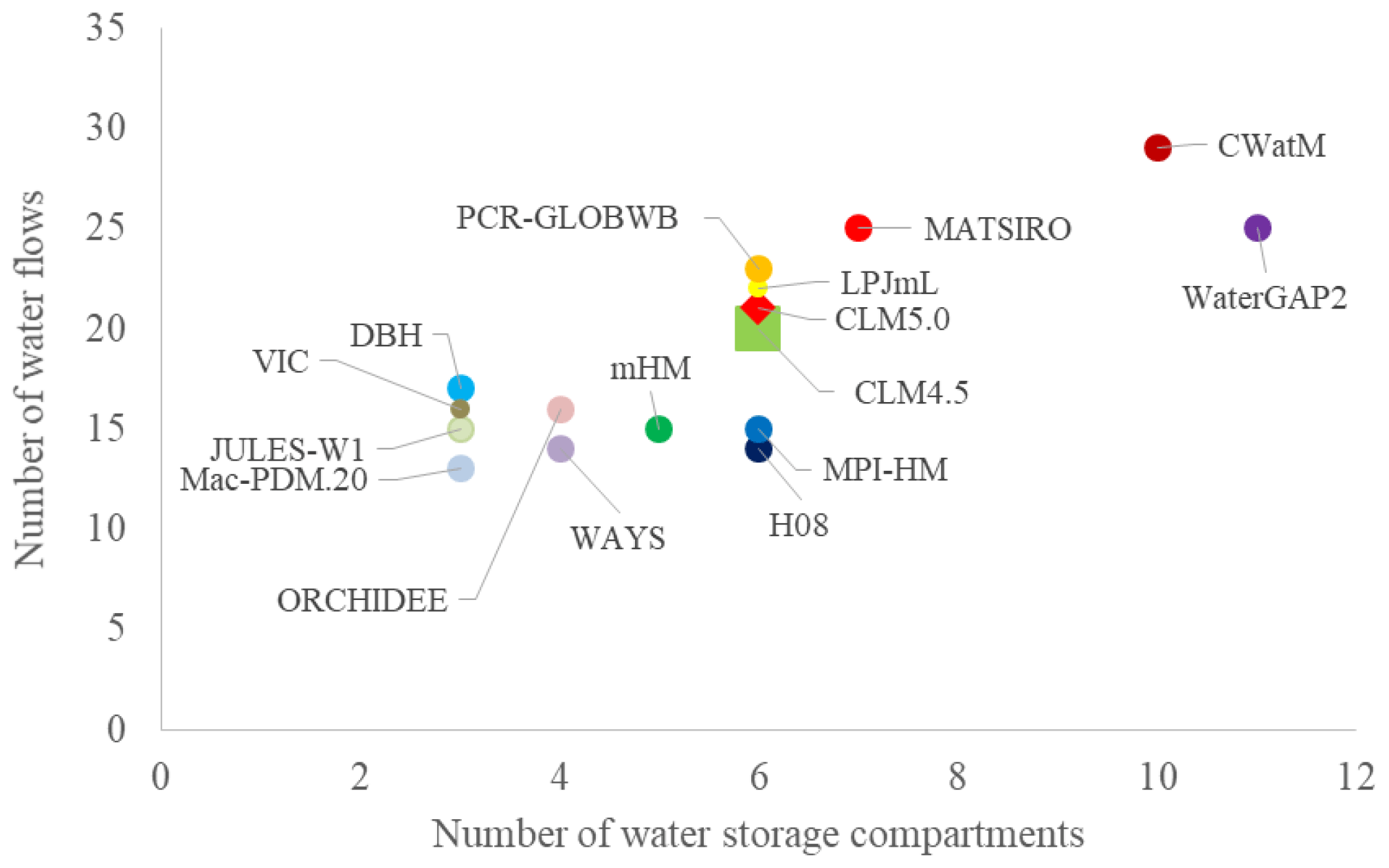
Figure 5Number of water storage compartments and water flows included in the ISIMIP2b global water models.
Among the nine GHMs, water flows range between 13 (Mac-PDM.20) and 29 (CWatM), and water storage compartments range between 3 (VIC and Mac-PDM.20) and 11 (WaterGAP2).
Among the six LSMs, water flows range between 15 (JULES-W1) and 25 (MATSIRO), and water storage compartments range between 3 (DBH and JULES-W1) and 7 (MATSIRO).
LPJmL, as a DGVM, simulated 22 water flows and 6 water storage compartments.
Seven models do not simulate water used by humans for economic purposes such as irrigation, domestic, livestock, manufacturing, electricity, and desalination (Fig. 6). Three models (CWatM, MATSIRO, and PCR-GLOBWB) combine the manufacturing and electricity sectors into one sector: the industry sector. WaterGAP2 simulates five human water use sectors: irrigation, domestic, livestock, manufacturing, and industry. Two models (PCR-GLOBWB and CWatM) simulate four human water use sectors: irrigation, domestic, livestock, and industry. H08 simulates four human water use sectors: irrigation, domestic, industry, and desalination. MATSIRO simulates three human water use sectors: irrigation, domestic, and industry. Four models (CLM4.5, CLM5.0, LPJmL, and MPI-HM) simulate only water used by humans for the irrigation sector. WaterGAP2 and CWatM have the highest number of water flows (23) to simulate human water use, while MPI-HM has the lowest number (3; Fig. 6). Among the five GHMs, water flows range between 3 (MPI-HM) and 23 (CWatM and WaterGAP2).
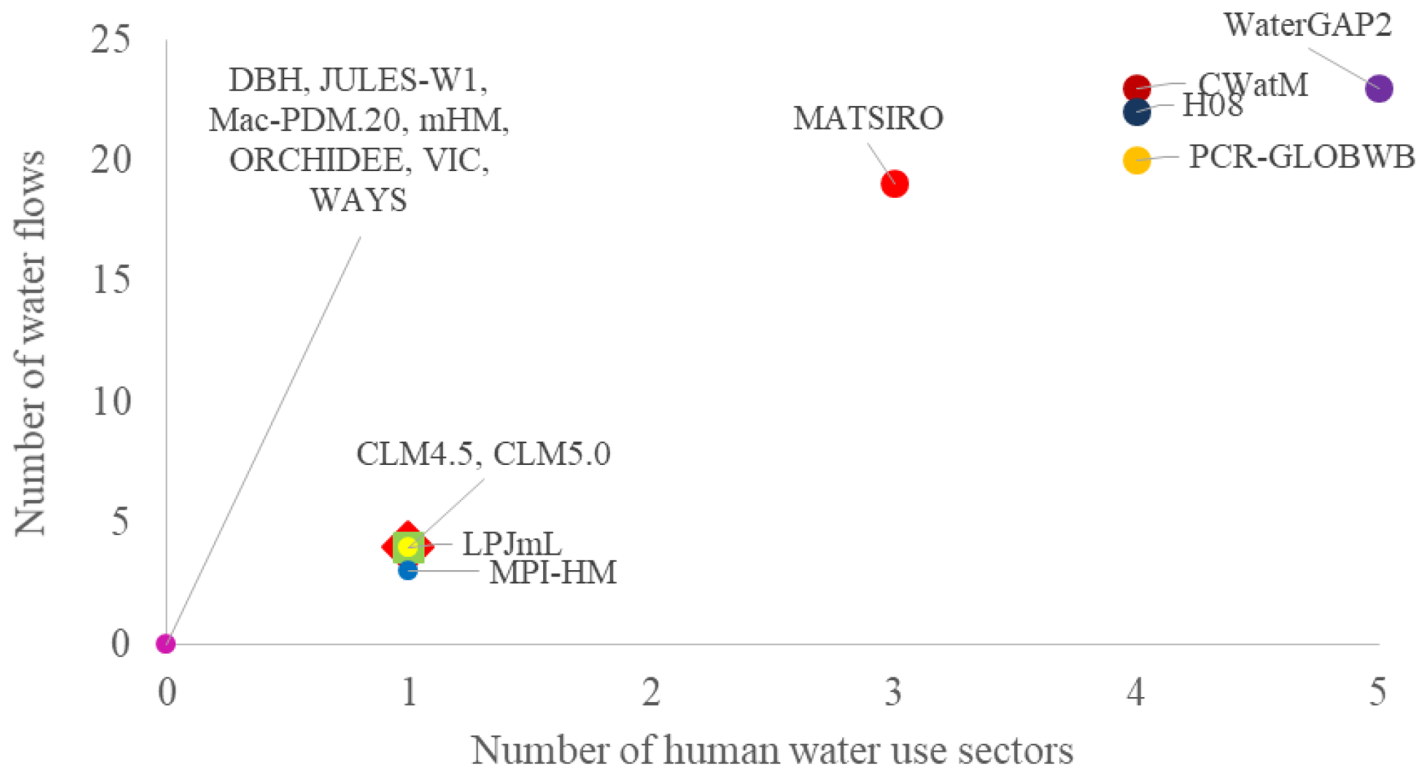
Figure 6Number of human water use sectors and related water flows included in the ISIMIP2b global water models.
Among the three LSMs, water flows range between 4 (CLM4.5 and CLM5.0) and 19 (MATSIRO).
LPJmL used four water flows to simulate the irrigation sector.
Ultimately, GWMs include similar processes in their structure, but they are lacking other processes, mentioned in Sect. 5, or include other processes, resulting in different model structures, or have used other parameter values determining various model results (Figs. 3 and 4). Therefore, in Sect. 7 we present future research on model development of 16 modelling groups involved in the present study.
Each model analysed in this study is continuously updated with the purpose of improving simulations. Therefore, in this section, we summarize model developments done outside the ISIMIP framework and potential future research of 16 GWMs (Tables S95 and S96). Each modelling team collected and provided these model developments. Some of the 16 analysed GWMs include, in their original structure, additional water storage compartments, water flows, and human water use sectors that have not been used for ISIMIP2b. Additional information on the 16 analysed GWMs can be found in the peer-reviewed articles mentioned in Table 11.

Some analysed GWMs have the ability to operate at various spatial and temporal scales: CWatM, CLM4.5, CLM5.0 (3 h time step at around 11 km).
The CLM team improved the irrigation scheme (Thiery et al., 2017, 2020), the extraction of groundwater (Felfelani et al., 2020), the representation of land cover and land management (Meier et al., 2018; Hirsch et al., 2017, 2018), and the implementation of reservoirs (Hauser et al., 2019). Numerous developments can be followed on the model's GitHub page (https://github.com/ESCOMP/CTSM, last access: 2 November 2020).
CWatM developed a groundwater scheme with linkages to MODFLOW for 5 arcmin and 30 arcsec spatial resolution. The CWatM modelling group plans to develop a reservoir storage including different operation schemes (e.g. energy, irrigation) to increase the temporal resolution (at 1 h) and to also apply a global calibration for ungauged catchments, such as using the Budyko framework (Greve et al., 2020), applying both the degree-day method and energy balance method to estimate snow accumulation and melt, and applying several methods to estimate evaporation based on changing CO2 concentration.
DBH plans to include human water uses (industrial and domestic sectors), either by developing a new module or using the simulations from other models (e.g. WFaS dataset), to calibrate the model in the new ISIMIP3 simulation round and to improve the input–output module to read and write netcdf files.
The H08 modelling team used an approximate Bayesian computation technique to calibrate four parameters that are transferred to other regions containing no observations, which are mainly based on Köppen–Geiger regions. The modelling group also increased the spatial resolution to 5 min and improved the representation of crops used for biofuel in the model.
The JULES-W1 modelling group plans to make a technical update that will enable the river routing module to estimate discharge.
The LPJmL group developed an improved energy balance module and soil hydrological scheme that can estimate permafrost dynamics (Schaphoff et al., 2013) and made the model source code freely available on GitHub (https://github.com/PIK-LPJmL/LPJmL, last access: 2 November 2020; Schaphoff et al., 2018), hoping to engage a broader scientific community in LPJmL model development and applications.
The Mac-PDM.20 modelling group plans to develop a water use module.
The MATSIRO modelling group has implemented a land use change process, terrestrial biogeochemical processes, and an additional crop growth process into MATSIRO to develop a new modelling framework. As key interactions are taken into account and all processes are coupled, important boundary conditions for hydrological simulations can be dynamically simulated internally. This hydrological simulation modelling framework has been coupled with MIROC GCM (global climate model) and has been used as an Earth system model. In addition, the group recently proposed new schemes for lateral groundwater flow, water temperature, and sediment transportation.
Ongoing efforts to improve the realism of hydrological processes in the mHM include the development of the multiscale lake module (mLM), a comprehensible framework for reservoir regulation and natural processes in lakes. Near-future developments will focus on a glacial module to better account for processes in cold regions, as well as coupling it to a groundwater model that will replace the current linear groundwater reservoir.
The MPI-HM modelling group plans to increase the spatial resolution of regional versions. The group is currently implementing canopy storage into the latest model version and is developing experiments to integrate reservoir storage.
The ORCHIDEE group is focusing on calibration, soil storage, groundwater storage, river storage, reservoir storage, and wetland storage (MacBean et al., 2020; Verbeke et al., 2019; Yin et al., 2020; Schrapffer et al., 2020; Mizuochi et al., 2021).
The PCR-GLOBWB modelling group plans to increase the temporal and spatial resolution of the input data, to increase the temporal resolution (3 h) for energy balance calculations and the global spatial resolution (1 km), to improve the soil representation by including the Richards equation, to add more snow elevation layers, to include additional fast runoff component for improving daily discharge simulations, and to improve the reservoir operating scheme (Sutanudjaja et al., 2018).
The VIC modelling group developed different irrigation practices (Shah et al., 2019a and b) and included a reservoir (Dang et al., 2020a and b) and a groundwater scheme in the model structure.
The WaterGAP2 modelling group plans to update the GRanD dataset used by the model, to include water temperature calculations, to couple the new developed groundwater model (Reinecke et al., 2019), and to update the non-irrigation water use datasets.
The WAYS modelling group plans to develop a new human water use module to consider agricultural, industrial, and domestic water use in the water cycle.
We assert that this study was realized through a multi-model intercomparison project (ISIMIP) and is based on communication and collaboration. Ideally, through a unified perspective and effective collaborations toward physically realistic hydrologic models (Clark et al., 2015a, 2017), communities will fill in existing knowledge gaps (Wagener, 2020), improve the quality of the input data and the processes in the models, and implement the missing processes in the models. In addition to these statements, we propose focusing the effective collaborations on effective “wish lists”, including specific research questions, goals to answer these questions, methods to achieve the goals, datasets to be used, tasks to be done, and, at the end of the project, a retrospective analysis on what has been done and what could be improved. Certainly, collaboration among these communities results in new multi-model intercomparison projects (MIPs) and multi-model ensembles that facilitate new analyses, comparisons, understandings, and improvements.
However, many studies highlighted the need to design hydrological inter-model comparison studies by nominating models or research questions according to some specific criteria (Gupta et al., 2008; M. P. Clark et al., 2011; Gupta et al., 2012), for example, (i) specific model compartments (Nazemi and Wheater, 2015; Wada et al., 2017); (ii) specific evaluation metrics (Gupta et al., 2009; Veldkamp et al., 2018; Zaherpour et al., 2018); and (iii) locations of specific hydrological indicators, regions, or rivers (Masaki et al., 2017; Veldkamp et al., 2018).
In global water modelling, there are some more methodologies that can be tested to evaluate multi-model structures and model equations, which are also considered hypotheses on runoff generation, for example, the Rainfall-Runoff Modelling Toolbox (Wagener et al., 2001), the rejectionist framework (Vaché and McDonnell, 2006), the Framework for Understanding Structural Errors (FUSE, Clark et al., 2008), SUPERFLEX (Fenicia et al., 2011), the Catchment Modelling Framework (CMF, Kraft et al., 2011), and the Structure for Unifying Multiple Modelling Alternatives (SUMMA, Clark et al., 2015b and c). Other methodologies can be used to evaluate parameter values, such as the Model Parameter Estimation Experiment (MOPEX: Duan et al., 2006), the multiple-try DREAM(ZS) algorithm (Laloy and Vrugt, 2012), the Generalized Likelihood Uncertainty Estimation methodology (GLUE: Beven and Binley, 2014), perturbed parameter ensembles (Gosling, 2013), the Uncertainty Quantification Python Laboratory platform (UQ-PyL: Wang et al., 2016), and Multiscale Parameter Regionalization (MPR, Samaniego et al., 2010 and 2017). Thus, some existing methods might offer some solutions for reducing the high number of parameters and their values still found in global water models and for applying more reasonable regionalization schemes in global water research (Bierkens, 2015). Other methods can be found in frameworks proposed by Döll and Romero-Lankao (2017) and Kundzewicz et al. (2018).
We recommend, for the benefit of the MIPs, (1) to maintain very good documentation of the model code; (2) to always start research with a list, for example, with water storage compartments, flows, and human water use sectors included in the model structures; (3) to have clear definitions of the variables, water storage compartments, flows, and human use sectors, describing their role in the model exactly; (4) to have synonyms for variables, helping to show similarities and differences among models; (5) to collect all ideas, recommendations, and improvements received from everyone (in our case, they were required to complete our study); (6) to collaborate and communicate with peers, which was very useful in our study for identifying synonyms among communities; (7) to describe your model or a model through your eyes and other's eyes to identify differences in terminology and assumptions in model code and similarities and differences among the models; and (8) to invest a large amount of time and patience and be meticulous about extracting equations of water storage, flow, and human water use sectors from the model code.
We encourage communities to write and convey a clear, simple, and understandable text for large audiences. We consider that simplicity improves communication, and communication starts with a common language, i.e. the same words having the same meaning for the sender and the receiver. While trivial in theory, in practice there are some discrepancies among scientists, as well as between scientists and stakeholders by using vocabulary differently in climate impact science (Sultan et al., 2020).
Our future research will include describing the GWMs analysed in this study through a standard visualization of the water cycle that will show the water storage compartments, water flows, and human water use sectors included in the ISIMIP2b model structures. These diagrams would be connected with the tables presented in the Supplement of the present paper (Tables S1–S83). Another future study might focus on the numerical implementation of each model code.
We note that this review and description study had a positive impact on the modelling groups, motivating them to re-think and re-analyse model structures, equations, and descriptions. We affirm that ISMIP global water sector needs to organize workshops on some parameterization experiments by changing model parameter values. Other evaluation studies could focus on the equations applied to compute water compartments, water flows, and human water use sectors, as well as considering model outputs, to identify the effect of different water compartments on model results. ISIMIP community could increase the number of regional and pilot studies (which could validate global studies) and the number of cross-sectoral climate impact assessments.
Certainly, simulating the terrestrial water cycle on the global scale involves many challenges, as we presented in this study. Other challenges have also been synthesized by reviewing articles published by the climate, global hydrological, and vegetation communities and have been classified according to the 23 unsolved problems in hydrology (UPH) identified by Blöschl et al. (2019) (Table S97). In summary, these challenges can generally be overcome through innovative and creative collaboration among communities and investment in technical infrastructure. In the end, Arheimer et al. (2020) showed that the catchment models can be applied at a global scale because of the new global datasets, increased computational capacity, new methods to estimate parameters, and collaboration. Ultimately, specific features of GWMs such as dam operation, human water abstractions, routing approaches, and calibration might become a part of Earth system models (Wood et al., 2011; Bierkens et al., 2015).
Global water models are used to simulate the climate–water–human system. However, recent evaluation studies show that there is a need to better simulate this system by including other hydrological processes, data on physical infrastructure, societal behaviour, cultural behaviour, water diversions, and virtual water, as well as by identifying its teleconnections on the global scale (Zaherpour et al., 2018; Veldkamp et al., 2018; Wada et al., 2017). Some studies also underline the need to better explain various model results and better understand how models work (Reinecke et al., 2021; Pokhrel et al., 2021).
We undertook the present study mainly to find similarities and differences among global water models that will facilitate interpretation of various results, as well as those of further intercomparison studies. We developed a standard equation writing style to achieve this goal. We found that there are some similarities among the models when applying similar equations for the same hydrological processes; however, model structures are different and various values have been used for parameters or variables.
In summary, we mention that our approach was affected by models' complexity and is limited to eight water storage compartments and their flows and mainly five human water use sectors because of models' complexity. We conclude that the standard writing style of the equations is useful and necessary for finding similarities and differences among models for each water storage, human water use sector, and water flow. In addition, it can be leveraged for explaining the different model outputs, for classification of the models based on cluster analysis, and for selecting the right model for the right application. It can also be used for drawing a standard schematic visualization of the water cycle, for describing models on ISIMIP and ISIpedia platforms (the open climate impacts encyclopedia, a part of the ISIMIP, https://www.isipedia.org/, last access: 2 November 2020), and for understanding how models work. Other modelling teams can apply, in their studies, our lists with water storage compartments, flows, and human water use sectors and the symbols presented in the Supplement. They can follow our steps in creating a standardized writing style of model equations, and they may be aware of some challenges that they could encounter. This study represents a roadmap in finding similarities and differences among models. However, it should be noted that these equations are available only for model versions used for ISIMIP2b.
We consider this study a blueprint for other studies because it offers a practical approach to identify similarities and differences among models that are necessary for a better interpretation of their various results.
We highlight the need to undertake experiments on individual water compartments in order to analyse the equations and parameters used, as well as the results obtained. We also underline the need to make multi-model intercomparison projects. This is because they enhance collaboration and communication between modelling groups, communities, countries and cultures, These projects, through communication and collaboration, also enhance creativity and open opportunities for finding new ways to improve the models.
Information on the availability of source code for the models featured in this article can be found in the Table 11.
No data were used in the writing of this paper.
Tables with equations for each water storage, water flow, and human water use sector; datasets used by global water models; models' structures; and future research perspectives can all be found in the Supplement. The supplement related to this article is available online at: https://doi.org/10.5194/gmd-14-3843-2021-supplement.
CET proposed, designed, and led the conceptualization of ISIMIP2b models' intercomparison based on their water cycle simulation and also conceptualized the standard writing style of their equations. The initial idea to compare the ISIMIP2b models based on their equations and a standard diagram was proposed by HMS, who also gave recommendations to the paper project. CET, WT, GL, PB, OR, TS, TT, FH, SR, and HMS provided LaTeX support to write equations on the Overleaf platform. HMS, WT, GL, PB, XL, JESB, LSA, MG, YS, OR, TS, JC, NW, HLS, TT, and GM checked the code and provided models' equations for each water storage and water flow. CET, HMS, WT, GL, PB, XL, JESB, LPS, MG, YS, OR, TS, JC, NW, HLS, TT, GM, AK, YP, LS, YW, VM, JL, PD and NH checked the consistency and correctness of the equations. HMS, WT, GL, PB, XL, JESB, LPS, MG, YS, OR, TS, JC, NW, HLS, and GM ran simulations for the ISIMIP2b project. SNG and HMS coordinated the ISIMIP2b model simulations of the global water sector. CET conducted the analysis, visualization, and wrote the original draft. AG and FZ provided recommendations for the manuscript. In this paper, all 16 global water models are equal, therefore, the coauthors are listed in the alphabetical order of the models: CLM4.5 – WT, CLM5.0 – GL, CWatM – PB, DBH – XL, H08 – JESB, LPJmL – LSA, JULES-W1 – MG, Mac-PDM.20 – SNG, MATSIRO – YS, mHM – OR, MPI-HM – TS, ORCHIDEE – JC, PCR-GLOBWB – NW, VIC – HLS, WaterGAP2 – TT, WAYS – GM. All authors reviewed, commented on, and contributed to the final draft.
The authors declare that they have no conflict of interest.
The present study was possible through the international ISIMIP framework. Camelia-Eliza Telteu and Hannes Müller Schmied are supported by the German Federal Ministry of Education and Research (grant no. 01LS1711F). Guoyong Leng is supported by the National Key Research and Development Program of China (no. 2020YFA0608502) and the National Natural Science Foundation of China (no. 42077420). Yadu Pokhrel received support from the National Science Foundation (CAREER Award; grant no. 1752729). Junguo Liu have been supported by the National Natural Science Foundation of China (grant no. 41625001), the Strategic Priority Research Program of the Chinese Academy of Sciences (grant no. XDA20060402), and High-level Special Funding of the Southern University of Science and Technology (grant no.G02296302, G02296402). Ganquan Mao is supported by the National Key R&D Program of China (grant no. 2017YFA0603704).
We thank to Jacob Schewe, Agnès Ducharne, Lukas Gudmundsson, and Lamprini Papadimitriou for their useful recommendations regarding the manuscript. We also thank to the ISIMIP coordination team for providing funds for the ISIMIP2b Global Water Paper-writing Workshop (30 July–1 August 2018), Frankfurt am Main, Germany; the Cross-sectoral ISIMIP Workshop 2019 (4 June 2019), where this paper could be discussed; and the ISIpedia Stakeholder Engagement Team (Inga Menke, Quentin Lejeune, Gina Maskell, Kaylin Lee) and ISIpedia stakeholders (Anatolii Shmurak, Atiq Kainan Ahmed, Aimé Koudou) for providing useful recommendations about the creation of the standard visualization of the water cycle simulated by the models analysed in this article. We are grateful for valuable comments and suggestions received from Wouter Knoben and Laura Devitt that helped to streamline and improve the consistency of the paper.
This research and open-access publication were funded by the German Federal Ministry of Education and Research (grant no. 01LS1711F).
This paper was edited by Jeffrey Neal and reviewed by Laura Devitt and Wouter Knoben.
Abbott, B. W., Bishop, K., Zarnetske, J. P., Hannah, D. M., Frei, R. J., Minaudo, C., Stuart, F. C., Krause, S., Conner, L., Ellison, D., Godsey, S. E., Plont, S., Marçais, J., Kolbe, T., Huebner, A., Hampton, T., Gu, S., Buhman, M., Sayedi, S. S., Ursache, O., Chapin, M., Henderson, K. D., and Pinay, G.: A water cycle for the Anthropocene, Hydrol. Process., 33, 3046–3052, https://doi.org/10.1002/hyp.13544, 2019.
Archfield, S. A., Clark, M. P., Arheimer, B., Hay, L. E., McMillan, H., Kiang, J. E., Seibert, J., Hakala, K., Bock, A., Wagener, T., Farmer, W. H., Andreassian, V., Attinger, S., Viglione, A., Knight, R., Markstrom, S., and Over, T.: Accelerating advances in continental domain hydrologic modeling. Water Resour. Res., 40, 10078–10091, https://doi.org/10.1002/2015WR017498, 2015.
Arheimer, B., Pimentel, R., Isberg, K., Crochemore, L., Andersson, J. C. M., Hasan, A., and Pineda, L.: Global catchment modelling using World-Wide HYPE (WWH), open data, and stepwise parameter estimation, Hydrol. Earth Syst. Sci., 24, 535–559, https://doi.org/10.5194/hess-24-535-2020, 2020.
Beck, H. E., van Dijk, A. I. J. M., de Roo, A., Miralles, D. G., McVicar, T. R., Schellekens, J., and Bruijnzeel, L. A.: Global-scale regionalization of hydrologic model parameters, Water Resour. Res., 52, 3599–3622, https://doi.org/10.1002/2015WR018247, 2016.
Bergström, S.: Development and application of a conceptual runoff model for Scandinavian catchments, SMHI Report RHO 7, Norrköping, 134 pp., 1976.
Best, M. J., Pryor, M., Clark, D. B., Rooney, G. G., Essery, R. L. H., Ménard, C. B., Edwards, J. M., Hendry, M. A., Porson, A., Gedney, N., Mercado, L. M., Sitch, S., Blyth, E., Boucher, O., Cox, P. M., Grimmond, C. S. B., and Harding, R. J.: The Joint UK Land Environment Simulator (JULES), model description – Part 1: Energy and water fluxes, Geosci. Model Dev., 4, 677–699, https://doi.org/10.5194/gmd-4-677-2011, 2011.
Beven, K: Rainfall-Runoff Modelling – The Primer, 2nd edn., Lancaster University, UK, Wiley-Blackwell, A John Wiley & Sons, Ltd., Publication, The Atrium, Southern Gate, Chichester, West Sussex, PO198SQ, UK, 2012.
Beven, K. and Binley, A.: GLUE: 20 years on, Hydrol. Process. 28, 5897–5918, https://doi.org/10.1002/hyp.10082, 2014.
Beven, K. J. and Kirby, M. J.: A physically based, variable contributing area model of basin hydrology / Un modèle à base physique de zone d'appel variable de l'hydrologie du bassin versant, Hydrolog. Sci. J., 24, 43–69, https://doi.org/10.1080/02626667909491834, 1979.
Beven, K. and Young, P.: A guide to good practice in modeling semantics for authors and referees, Water Resour. Res., 49, 5092–5098, https://doi.org/10.1002/wrcr.20393, 2013.
Bicheron, P., Amberg, V., Bourg, L., Petit, D., Huc, M., Miras, B., Brockmann, C., Hagolle, O., Delwart, S., Ranera, F., Leroy, M., and Arino, O: Geolocation Assessment of MERIS GlobCover Orthorectified Products, IEEE Transactions on Geoscience and Remote Sensing, 49, 2972–2982, https://doi.org/10.1109/TGRS.2011.2122337, 2011.
Biemans, H., Haddeland, I., Kabat, P., Ludwig, F., Hutjes, R. W. A, Heinke, J., Von Bloh, W., and Gerten, D.: Impact of reservoirs on river discharge and irrigation water supply during the 20th century, Water Resour. Res., 47, W03509, https://doi.org/10.1029/2009WR008929, 2011.
Bierkens, M. F. P.: Global hydrology 2015: State, trends, and directions, Water Resour. Res., 51, 7, 4923–4947, https://doi.org/10.1002/2015WR017173, 2015.
Bierkens, M. F. P. and van Geer, F. C.: Stochastic Hydrology, Department of Physical Geography, Utrecht University, 237 pp., available at: http://www.earthsurfacehydrology.nl/wp-content/uploads/2012/01/Syllabus_Stochastic-Hydrology.pdf (last access: 2 November 2020), 2007.
Bierkens, M. F. P., Bell, V. A., Burek, P., Chaney, N., Condon, L. E., David, C. H., de Roo, A., Döll, P., Drost, N., Famiglietti, J. S., Flörke, M., Gochis, D. J., Houser, P., Hut, R., Keune, J., Kollet, S., Maxwell, R. M., Reager, J. T., Samaniego, L., Sudicky, E., Sutanudjaja, E. H., van de Giesen, N., Winsemius, H., and Wood, E. F.: Hyper-resolution global hydrological modelling: what is next?, Hydrol. Process., 29, 2, 310–320, https://doi.org/10.1002/hyp.10391, 2015.
Blöschl, G., Bierkens, M. F. P., Chambel, A., Cudennec, C., Destouni, G., Fiori, A., Kirchner, J. W., McDonnell, J. J., Savenije, H. H. G., Sivapalan, M., Stumpp, C., Toth, E., Volpi, E., Carr, G., Lupton, C., Salinas, J., Széles, B., Viglione, A., Aksoy, H., Allen, S. T., Amin, A., Andréassian, V., Arheimer, B., Aryal, S. K., Baker, V., Bardsley, E., Barendrecht, M. H., Bartosova, A., Batelaan, O., Berghuijs, W. R., Beven, K., Blume, T., Bogaard, T., Borges de Amorim, P., Böttcher, M. E., Boulet, G., Breinl, K., Brilly, M., Brocca, L., Buytaert, W., Castellarin, A., Castelletti, A., Chen, X., Chen, Y., Chen, Y., Chifflard, P., Claps, P., Clark, M. P., Collins, A. L., Croke, B., Dathe, A., David, P. C., de Barros, F. P. J., de Rooij, G., Di Baldassarre, G., Driscoll, J. M., Duethmann, D., Dwivedi, R., Eris, E., Farmer, W. H., Feiccabrino, J., Ferguson, G., Ferrari, E., Ferraris, S., Fersch, B., Finger, D., Foglia, L., Fowler, K., Gartsman, B., Gascoin, S., Gaume, E., Gelfan, A., Geris, J., Gharari, S., Gleeson, T., Glendell, M., Gonzalez Bevacqua, A., González-Dugo, M. P., Grimaldi, S., Gupta, A. B., Guse, B., Han, D., Hannah, D., Harpold, A., Haun, S., Heal, K., Helfricht, K., Herrnegger, M., Hipsey, M., Hlaváčiková, H., Hohmann, C., Holko, L., Hopkinson, C., Hrachowitz, M., Illangasekare, T. H., Inam, A., Innocente, C., Istanbulluoglu, E., Jarihani, B., Kalantari, Z., Kalvans, A., Khanal, S., Khatami, S., Kiesel, J., Kirkby, M., Knoben, W., Kochanek, K., Kohnová, S., Kolechkina, A., Krause, S., Kreamer, D., Kreibich, H., Kunstmann, H., Lange, H., Liberato, M. L. R., Lindquist, E., Link, T., Liu, J., Loucks, D. P., Luce, C., Mahé, G., Makarieva, O., Malard, J., Mashtayeva, S., Maskey, S., Mas-Pla, J., Mavrova-Guirguinova, M., Mazzoleni, M., Mernild, S., Misstear, B. D., Montanari, A., Müller-Thomy, H., Nabizadeh, A., Nardi, F., Neale, C., Nesterova, N., Nurtaev, B., Odongo, V. O., Panda, S., Pande, S., Pang, Z., Papacharalampous, G., Perrin, C., Pfister, L., Pimentel, R., Polo, M. J., Post, D., Sierra, C. P., Ramos, M.-H., Renner, M., Reynolds, J. E., Ridolfi, E., Rigon, R., Riva, M., Robertson, D. E., Rosso, R., Roy, T. Sá, J. H. M., Salvadori, G., Sandells, M., Schaefli, B., Schumann, A., Scolobig, A., Seibert, J., Servat, E., Shafiei, M., Sharma, A., Sidibe, M., Sidle, R. C., Skaugen, T., Smith, H., Spiessl, S. M., Stein, L., Steinsland, I., Strasser, U., Su, B., Szolgay, J., Tarboton, D., Tauro, F., Thirel, G., Tian, F., Tong, R., Tussupova, K., Tyralis, H., Uijlenhoet, R., van Beek, R., van der Ent, R. J., van der Ploeg, M., Van Loon, A. F., van Meerveld, I., van Nooijen, R., van Oel, P. R., Vidal, J.-P., von Freyberg, J., Vorogushyn, S., Wachniew, P., Wade, A. J., Ward, P., Westerberg, I. K., White, C., Wood, E. F., Woods, R., Xu, Z., Yilmaz, K. K., and Zhang, Y.: Twentythree Unsolved Problems in Hydrology (UPH) – a community perspective, Hydrolog. Sci. J., 64, 1141–1158, https://doi.org/10.1080/02626667.2019.1620507, 2019.
Bondeau, A., Pascalle, C. S., Sönke, Z., Schaphoff, S., Lucht, W., Cramer, W., Gerten, D., Lotze-Campen, H., Müller, C., Reichstein, M., and Smith, B.: Modelling the role of agriculture for the 20th century global terrestrial carbon balance, Glob. Change Biol., 13, 679–706, https://doi.org/10.1111/j.1365-2486.2006.01305.x, 2007.
Bouaziz, L. J. E., Fenicia, F., Thirel, G., de Boer-Euser, T., Buitink, J., Brauer, C. C., De Niel, J., Dewals, B. J., Drogue, G., Grelier, B., Melsen, L. A., Moustakas, S., Nossent, J., Pereira, F., Sprokkereef, E., Stam, J., Weerts, A. H., Willems, P., Savenije, H. H. G., and Hrachowitz, M.: Behind the scenes of streamflow model performance, Hydrol. Earth Syst. Sci., 25, 1069–1095, https://doi.org/10.5194/hess-25-1069-2021, 2021.
Brunner, M., Pool, S., Kiewiet, L., and Acheson, E: The other's perception of a streamflow sample: From a bottle of water to a data point, Hydrol. Process., 32, 2922–2927, https://doi.org/10.1002/hyp.13227, 2018.
Burek, P., Smilovic, M., Satoh, Y., Kahil, T., Guillaumot, L., Tang, T., Greve, P., and Wada, Y.: Community Water Model (CwatM) (Version v1.04), Zenodo, https://doi.org/10.5281/zenodo.3361478, 2019.
Burek, P., Satoh, Y., Kahil, T., Tang, T., Greve, P., Smilovic, M., Guillaumot, L., Zhao, F., and Wada, Y.: Development of the Community Water Model (CWatM v1.04) – a high-resolution hydrological model for global and regional assessment of integrated water resources management, Geosci. Model Dev., 13, 3267–3298, https://doi.org/10.5194/gmd-13-3267-2020, 2020.
Chow, V. T., Maidment, D. R., and Mays, L. W.: Applied hydrology, McGraw-Hill, New York, 1998.
Clark, D. B., Mercado, L. M., Sitch, S., Jones, C. D., Gedney, N., Best, M. J., Pryor, M., Rooney, G. G., Essery, R. L. H., Blyth, E., Boucher, O., Harding, R. J., Huntingford, C., and Cox, P. M.: The Joint UK Land Environment Simulator (JULES), model description – Part 2: Carbon fluxes and vegetation dynamics, Geosci. Model Dev., 4, 701–722, https://doi.org/10.5194/gmd-4-701-2011, 2011.
Clark, M. P., Slater, A. G., Rupp, D. E., Woods, R. A., Vrugt, J. A., Gupta, H. V., Wagener, T., and Hay, L. E.: Framework for Understanding Structural Errors (FUSE): A modular framework to diagnose differences between hydrological models, Water Resour. Res., 44, W00B02, https://doi.org/10.1029/2007WR006735, 2008.
Clark, M. P., Kavetski, D., and Fenicia, F.: Pursuing the method of multiple working hypotheses for hydrological modeling, Water Resour. Res., 47, W09301, https://doi.org/10.1029/2010WR009827, 2011.
Clark, M. P., Fan, Y., Lawrence, D. M., Adam, J. C., Bolster, D., Gochis, D. J., Hooper, R. P., Kumar, M., Leung, L. R., Mackay, D. S., Maxwell, R. M., Shen, C., Swenson, S. C., and X. Zeng: Improving the representation of hydrologic processes in Earth System Models, Water Resour. Res., 51, 5929–5956, https://doi.org/10.1002/2015WR017096, 2015a.
Clark, M. P., Nijssen, B., Lundquist, J. D., Kavetski, D., Rupp, D. E., Woods, R. A., Freer, J. E., Gutmann, E. D., Wood, A. W., Brekke, L. D., Arnold, J. R., Gochis, D. J., and Rasmussen, R. M.: A unified approach for process-based hydrologic modeling: Part 1. Modeling concept, Water Resour. Res., 51, 2498–2514, https://doi.org/10.1002/2015WR017198, 2015b.
Clark, M. P., Nijssen, B., Lundquist, J. D., Kavetski, D., Rupp, D. E., Woods, R. A., Freer, J. E.,Gutmann, E. D., Wood, A. W., Gochis, D. J., Rasmussen, R. M., Tarboton, D. G., Mahat, V., Flerchinger, G. N., and Marks, D. G.: A unified approach for process-based hydrologic modeling: Part 2. Model implementation and case studies, Water Resour. Res., 51, 2515–2542, https://doi.org/10.1002/2015WR017200, 2015c.
Clark, M. P., Bierkens, M. F. P., Samaniego, L., Woods, R. A., Uijlenhoet, R., Bennett, K. E., Pauwels, V. R. N., Cai, X., Wood, A. W., and Peters-Lidard, C. D.: The evolution of process-based hydrologic models: historical challenges and the collective quest for physical realism, Hydrol. Earth Syst. Sci., 21, 3427–3440, https://doi.org/10.5194/hess-21-3427-2017, 2017.
CTSM Development Team: ESCOMP/CTSM: Update documentation for release-clm5.0 branch, and fix issues with no-anthro surface dataset creation (Version release-clm5.0.34), Zenodo, https://doi.org/10.5281/zenodo.3779821, 2020.
Cucchi, M., Weedon, G. P., Amici, A., Bellouin, N., Lange, S., Müller Schmied, H., Hersbach, H., and Buontempo, C.: WFDE5: bias-adjusted ERA5 reanalysis data for impact studies, Earth Syst. Sci. Data, 12, 2097–2120, https://doi.org/10.5194/essd-12-2097-2020, 2020.
Dang, T. D., Chowdhury, A. F. M. K., and Galelli, S.: On the representation of water reservoir storage and operations in large-scale hydrological models: implications on model parameterization and climate change impact assessments, Hydrol. Earth Syst. Sci., 24, 397–416, https://doi.org/10.5194/hess-24-397-2020, 2020a.
Dang, T. D., Vu, D. T., Chowdhury, A. F. M. K., and Galelli, S.: A software package for the representation and optimization of water reservoir operations in the VIC hydrologic model, Environ. Modell. Softw., https://doi.org/10.1016/j.envsoft.2020.104673, 2020b.
de Boer-Euser, T., Bouaziz, L., De Niel, J., Brauer, C., Dewals, B., Drogue, G., Fenicia, F., Grelier, B., Nossent, J., Pereira, F., Savenije, H., Thirel, G., and Willems, P.: Looking beyond general metrics for model comparison – lessons from an international model intercomparison study, Hydrol. Earth Syst. Sci., 21, 423–440, https://doi.org/10.5194/hess-21-423-2017, 2017.
Döll, P. and Fiedler, K.: Global-scale modeling of groundwater recharge, Hydrol. Earth Syst. Sci., 12, 863–885, https://doi.org/10.5194/hess-12-863-2008, 2008.
Döll, P. and Lehner, B.: Validation of a new global 30-min drainage direction map, J. Hydrol., 258, 214–231, https://doi.org/10.1016/S0022-1694(01)00565-0, 2002.
Döll, P. and Romero-Lankao, P.: How to embrace uncertainty in participatory climate change risk management – A roadmap, Earth's Future, 5, 18–36, https://doi.org/10.1002/2016EF000411, 2017.
Döll, P., Kaspar, F., and Lehner, B.: A global hydrological model for deriving water availability indicators: model tuning and validation, J. Hydrol., 270, 105–134, https://doi.org/10.1016/S0022-1694(02)00283-4, 2003.
Döll, P., Fiedler, K., and Zhang, J.: Global-scale analysis of river flow alterations due to water withdrawals and reservoirs, Hydrol. Earth Syst. Sci., 13, 2413–2432, https://doi.org/10.5194/hess-13-2413-2009, 2009.
Döll, P., Hoffmann-Dobrev, H., Portmann, F. T., Siebert, S., Eicker, A., Rodell, M., Strassberg, G., and Scanlon, B. R.: Impact of water withdrawals from groundwater and surface water on continental water storage variations, J. Geodyn., 59–60, 143–156, https://doi.org/10.1016/j.jog.2011.05.001, 2012.
Döll, P., Müller Schmied, H., Schuh, C., Portmann, F. T., and Eicker, A.: Global-scale assessment of groundwater depletion and related groundwater abstractions: Combining hydrological modelling with information from well observations and GRACE satellites, Water Resour. Res., 50, 5698–5720, https://doi.org/10.1002/2014WR015595, 2014.
Döll, P., Douville, H., Güntner, A., Müller Schmied, H., and Wada, Y.: Modelling Freshwater Resources at the Global Scale: Challenges and Prospects, Surv. Geophys., 37, 195–221, https://doi.org/10.1007/s10712-015-9343-1, 2016.
Duan, Q., Schaake, J., Andreassian, V., Franks, S., Goteti, G., Gupta, H. V., Gusev, Y. M., Habets, F., Hall, A., Hay, L., Hogue, T., Huang, M., Leavesley, G., Liang, X., Nasonova, O. N., Noilhan, J., Oudin, L., Sorooshian, S., Wagener, T., and Wood, E. F.: Model parameter estimation experiment (MOPEX): an overview of science strategy and major results from the second and third workshops, J. Hydrol., 320, 3–17, https://doi.org/10.1016/j.jhydrol.2005.07.031, 2006.
Ducoudré, N. I., Laval, K., and Perrier, A.: SECHIBA, a New Set of Parameterizations of the Hydrologic Exchanges at the Land-Atmosphere Interface within the LMD Atmospheric General Circulation Model, J. Climate, 6, 248–273, https://doi.org/10.1175/1520-0442(1993)006<0248:SANSOP>2.0.CO;2, 1993.
Duethmann, D., Blöschl, G., and Parajka, J.: Why does a conceptual hydrological model fail to correctly predict discharge changes in response to climate change?, Hydrol. Earth Syst. Sci., 24, 3493–3511, https://doi.org/10.5194/hess-24-3493-2020, 2020.
Dümenil, L. and Todini, E.: A rainfall-runoff scheme for use in the Hamburg climate model, in: Advances in Theoretical Hydrology: A tribute to James Dooge, edited by: O'Kane, J. P., Amsterdam: Elsevier Science Publishers B. V., 129–157, available at: http://hdl.handle.net/11858/00-001M-0000-0029-CE00-5 (last access: 2 November 2020), 1992.
Essery, R., Morin, S., Lejeune, Y., and Ménard, C. B.: A comparison of 1701 snow models using observations from an alpine site, Advances in water resources, 55, 131–148, https://doi.org/10.1016/j.advwatres.2012.07.013, 2013.
Eyring, V., Bony, S., Meehl, G. A., Senior, C. A., Stevens, B., Stouffer, R. J., and Taylor, K. E.: Overview of the Coupled Model Intercomparison Project Phase 6 (CMIP6) experimental design and organization, Geosci. Model Dev., 9, 1937–1958, https://doi.org/10.5194/gmd-9-1937-2016, 2016.
FAO/IIASA/ISRIC/ISSCAS/JRC: Harmonized World Soil Database (version 1.2), FAO, Rome, Italy and IIASA, Laxenburg, Austria, available at: https://webarchive.iiasa.ac.at/Research/LUC/External-World-soil-database/HTML/ (last access: 10 June 2021), 2012.
Farthing, M. W. and Ogden, F. L.: Numerical Solution of Richards' Equation: A Review of Advances and Challenges, Soil Sci. Soc. Am. J., 81, 1257–1269, https://doi.org/10.2136/sssaj2017.02.0058, 2017.
Fekete, B. M., Vörösmarty, C. J., Hall, F. G., Collatz, G. J., Meeson, B. W., Los, S. O., Brown De Colstoun, E., and Landis, D. R.: ISLSCP II UNH/GRDC Composite Monthly Runoff, ORNL DAAC, Oak Ridge, Tennessee, USA, https://doi.org/10.3334/ORNLDAAC/994, 2011.
Felfelani, F., Lawrence, D. M., and Pokhrel, Y.: Representing intercell lateral groundwater flow and aquifer pumping in the community land model, Water Resour. Res., 56, e2020WR027531, https://doi.org/10.1029/2020WR027531, 2020.
Fenicia, F., Kavetski, D., and Savenije, H. H. G: Elements of a flexible approach for conceptual hydrological modeling: 1. Motivation and theoretical development, Water Resour. Res., 47, W11510, https://doi.org/10.1029/2010WR010174, 2011.
Flörke, M., Kynast, E., Bärlund, I., Eisner, S., Wimmer, F., and Alcamo, J.: Domestic and industrial water uses of the past 60 years as a mirror of socio-economic development: A global simulation study, Global Environ. Change, 23, 144–156, https://doi.org/10.1016/j.gloenvcha.2012.10.018, 2013.
Frieler, K., Lange, S., Piontek, F., Reyer, C. P. O., Schewe, J., Warszawski, L., Zhao, F., Chini, L., Denvil, S., Emanuel, K., Geiger, T., Halladay, K., Hurtt, G., Mengel, M., Murakami, D., Ostberg, S., Popp, A., Riva, R., Stevanovic, M., Suzuki, T., Volkholz, J., Burke, E., Ciais, P., Ebi, K., Eddy, T. D., Elliott, J., Galbraith, E., Gosling, S. N., Hattermann, F., Hickler, T., Hinkel, J., Hof, C., Huber, V., Jägermeyr, J., Krysanova, V., Marcé, R., Müller Schmied, H., Mouratiadou, I., Pierson, D., Tittensor, D. P., Vautard, R., van Vliet, M., Biber, M. F., Betts, R. A., Bodirsky, B. L., Deryng, D., Frolking, S., Jones, C. D., Lotze, H. K., Lotze-Campen, H., Sahajpal, R., Thonicke, K., Tian, H., and Yamagata, Y.: Assessing the impacts of 1.5 ∘C global warming – simulation protocol of the Inter-Sectoral Impact Model Intercomparison Project (ISIMIP2b), Geosci. Model Dev., 10, 4321–4345, https://doi.org/10.5194/gmd-10-4321-2017, 2017.
Friend, A. D., Lucht, W., Rademacher, T. T., Keribin, R., Betts, R., Cadule, P., Ciais, P., Clark, D. B., Dankers, R., Falloon, P. D. Ito, A., Kahana, A., Kleidoni, A., Lomasj, M. R., Nishinah, K., Ostbergb, S., Pavlicki, R., Peylinf, P., Schaphoffb, S., Vuichardf, N., Warszawskib, L., Wiltshired, A., and Woodwardj, F. I.: Carbon residence time dominates uncertainty in terrestrial vegetation responses to future climate and atmospheric CO2, P. Natl. Acad. Sci. USA, 111, 3280–3285, https://doi.org/10.1073/pnas.1222477110, 2014.
Gao, H., Tang, Q., Shi, X., Zhu, C., Bohn, T. J., Su, F., Sheffield, J., Pan, M., Lettenmaier, D. P., and Wood, E. F.: Water budget record from Variable Infiltration Capacity (VIC) model, Algorithm Theor. Basis Doc., Terr. Water Cycle Data Rec., available at: https://eprints.lancs.ac.uk/id/eprint/89407/1/Gao_et_al_VIC_2014.pdf (last access: 2 November 2020), 2009.
Gerten, D., Schaphoff, S., Haberlandt, U., Lucht, W., and Sitch, S.: Terrestrial vegetation and water balance – hydrological evaluation of a dynamic global vegetation model, J. Hydrol., 286, 249–270, https://doi.org/10.1016/j.jhydrol.2003.09.029, 2004.
Gosling, S. N.: Systematic quantification of climate change impacts modelling uncertainty, in: Impacts World 2013 International Conference on Climate Change Effects, Potsdam, Germany, 27–30 May 2013, 268–274, available at: https://gfzpublic.gfz-potsdam.de/rest/items/item_152514_5/component/file_152588/content (last access: 2 November 2020), 2013.
Gosling, S. N. and Arnell, N. W.: Simulating current global river runoff with a global hydrological model: Model revisions, validation, and sensitivity analysis, Hydrol. Process., 25, 1129–1145, https://doi.org/10.1002/hyp.7727, 2011.
Greve, P., Burek, P., and Wada, Y.: Using the Budyko Framework for Calibrating a Global Hydrological Model, Water Resour. Res., 56, e2019WR026280, https://doi.org/10.1029/2019WR026280, 2020.
Gudmundsson, L., Boulange, J., Do, H. X., Gosling, S. N., Grillakis, M. G., Koutroulis, A. G., Leonard, M., Liu, J., Müller Schmied, H., Papadimitriou, L., Pokhrel, Y., Seneviratne, S. I., Satoh, Y., Thiery, W., Westra, S., Zhang, X., and Zhao, F.: Globally observed trends in mean and extreme river flow attributed to climate change, Science, 371, 1159–1162, https://doi.org/10.1126/science.aba3996, 2021.
Guimberteau, M., Ducharne, A., Ciais, P., Boisier, J. P., Peng, S., De Weirdt, M., and Verbeeck, H.: Testing conceptual and physically based soil hydrology schemes against observations for the Amazon Basin, Geosci. Model Dev., 7, 1115–1136, https://doi.org/10.5194/gmd-7-1115-2014, 2014.
Guimberteau, M., Zhu, D., Maignan, F., Huang, Y., Yue, C., Dantec-Nédélec, S., Ottlé, C., Jornet-Puig, A., Bastos, A., Laurent, P., Goll, D., Bowring, S., Chang, J., Guenet, B., Tifafi, M., Peng, S., Krinner, G., Ducharne, A., Wang, F., Wang, T., Wang, X., Wang, Y., Yin, Z., Lauerwald, R., Joetzjer, E., Qiu, C., Kim, H., and Ciais, P.: ORCHIDEE-MICT (v8.4.1), a land surface model for the high latitudes: model description and validation, Geosci. Model Dev., 11, 121–163, https://doi.org/10.5194/gmd-11-121-2018, 2018.
Gupta, H. V., Wagener, T., and Liu, Y.: Reconciling theory withobservations: Elements of a diagnostic approach to model evaluation, Hydrol. Process., 22, 3802–3813, https://doi.org/10.1002/hyp.6989, 2008.
Gupta, H. V., Kling, H., Yilmaz, K. K., and Martinez-Baquero, G. F.: Decomposition of the mean squared error & NSE performance criteria: Implications for improving hydrological modelling, J. Hydrol., 377, 80–91, https://doi.org/10.1016/j.jhydrol.2009.08.003, 2009.
Gupta, H. V., Clark, M. P., Vrugt, J. A., Abramowitz, G., and Ye, M.: Towards a comprehensive assessment of model structural adequacy, Water Resour. Res., 48, W08301, https://doi.org/10.1029/2011WR011044, 2012.
Guseva, S., Bleninger, T., Jöhnk, K., Polli, B. A., Tan, Z., Thiery, W., Zhuang, Q., Rusak, J. A., Yao, H., Lorke, A., and Stepanenko, V.: Multimodel simulation of vertical gas transfer in a temperate lake, Hydrol. Earth Syst. Sci., 24, 697–715, https://doi.org/10.5194/hess-24-697-2020, 2020.
Haddeland, I., Clark, D. B., Franssen, W., Ludwig, F., Voß, F., Arnell, N. W., Bertrand, N., Best, M., Folwell, S., Gerten, D., Gomes, S., Gosling, S. N., Hagemann, S., Hanasaki, N., Harding, R., Heinke, J., Kabat, P., Koirala, S., Oki, T., Polcher, J., Stacke, T., Viterbo, P., Weedon, G. P., and Yeh, P.: Multimodel Estimate of the Global Terrestrial Water Balance: Setup and First Results, Water and Global Change (WATCH) special collection, 12, 869–884, https://doi.org/10.1175/2011JHM1324.1, 2011.
Hagemann, S.: An Improved Land Surface Parameter Dataset for Global and Regional Climate Models, Max-Planck-Institut für Meteorologie, MPI Report 336, available at: https://mpimet.mpg.de/fileadmin/publikationen/Reports/max_scirep_336.pdf (last access: 2 November 2020), ISSN 0937-1060, 2002.
Hanasaki, N.: H08 Version 20190101, Zenodo, https://doi.org/10.5281/zenodo.4263375, 2020.
Hanasaki, N., Kanae, S., and Oki, T.: A reservoir operation scheme for global river routing models, J. Hydrol., 327, 22–41, https://doi.org/10.1016/j.jhydrol.2005.11.011, 2006.
Hanasaki, N., Kanae, S., Oki, T., Masuda, K., Motoya, K., Shirakawa, N., Shen, Y., and Tanaka, K.: An integrated model for the assessment of global water resources – Part 1: Model description and input meteorological forcing, Hydrol. Earth Syst. Sci., 12, 1007–1025, https://doi.org/10.5194/hess-12-1007-2008, 2008.
Hanasaki, N., Yoshikawa, S., Pokhrel, Y., and Kanae, S.: A global hydrological simulation to specify the sources of water used by humans, Hydrol. Earth Syst. Sci., 22, 789–817, https://doi.org/10.5194/hess-22-789-2018, 2018.
Hauser, M., Thiery, W., and Seneviratne, S. I.: Potential of global land water recycling to mitigate local temperature extremes, Earth Syst. Dynam., 10, 157–169, https://doi.org/10.5194/esd-10-157-2019, 2019.
Hirsch, A. L., Wilhelm, M., Davin, E. L., Thiery, W., and Seneviratne, S. I.: Can climate-effective land management reduce regional warming?, J. Geophys. Res.-Atmos., 122, 2269–2288, https://doi.org/10.1002/2016JD026125, 2017.
Hirsch, A. L., Prestele, R., Davin, E. L., Seneviratne, S. I., Thiery, W., and Verburg, P. H.: Modelled biophysical impacts of conservation agriculture on local climates, Glob. Change Biol., 24, 4758–4774, https://doi.org/10.1111/gcb.14362, 2018.
Hunger, M. and Döll, P.: Value of river discharge data for global-scale hydrological modeling, Hydrol. Earth Syst. Sci., 12, 841–861, https://doi.org/10.5194/hess-12-841-2008, 2008.
Jung, M., Reichstein, M., Margolis, H. A., Cescatti, A., Richardson, A. D., Arain, M. A., Arneth, A., Bernhofer, C., Bonal, D., Chen, J., Gianelle, D., Gobron, N., Kiely, G., Kutsch, W., Lasslop, G., Law, B. E., Lindroth, A., Merbold, L., Montagnani, L., Moors, E. J., Papale, D., Sottocornola, M., Vaccari, F., and Williams, C.: Global patterns of land-atmosphere fluxes of carbon dioxide, latent heat, and sensible heat derived from eddy covariance, satellite, andmeteorological observations, J. Geophys. Res., 116, G00J07, https://doi.org/10.1029/2010JG001566, 2011.
Kageyama, M., Braconnot, P., Harrison, S. P., Haywood, A. M., Jungclaus, J. H., Otto-Bliesner, B. L., Peterschmitt, J.-Y., Abe-Ouchi, A., Albani, S., Bartlein, P. J., Brierley, C., Crucifix, M., Dolan, A., Fernandez-Donado, L., Fischer, H., Hopcroft, P. O., Ivanovic, R. F., Lambert, F., Lunt, D. J., Mahowald, N. M., Peltier, W. R., Phipps, S. J., Roche, D. M., Schmidt, G. A., Tarasov, L., Valdes, P. J., Zhang, Q., and Zhou, T.: The PMIP4 contribution to CMIP6 – Part 1: Overview and over-arching analysis plan, Geosci. Model Dev., 11, 1033–1057, https://doi.org/10.5194/gmd-11-1033-2018, 2018.
Klein Goldewijk, C. G. M.: Anthropogenic land-use estimates for the Holocene; HYDE 3.2, DANS [data set], https://doi.org/10.17026/dans-25g-gez3, 2017.
Koirala, S., Yeh, P. J.-F., Hirabayashi, Y., Kanae, S., and Oki, T.: Global-scale land surface hydrologic modeling with the representation of water table dynamics, J. Geophys. Res.-Atmos., 119, 75–89, https://doi.org/10.1002/2013JD020398, 2014.
Knutti, R., Masson, D., and Gettelman, A.: Climate model genealogy: Generation CMIP5 and how we got there, Geophys. Res. Lett., 40, 1194–1199, https://doi.org/10.1002/grl.50256, 2013.
Kraft, P., Vaché, K. B., Frede, H.-G., and Breuer, L.: CMF: A Hydrological Programming Language Extension For Integrated Catchment Models, Environ. Modell. Softw., 26, 828–830, https://doi.org/10.1016/j.envsoft.2010.12.009, 2011.
Krysanova, V., Wechsung, F., Arnold, J., Srinivasan, R., and Williams, J.: SWIM (Soil and Water Integrated Model) – User Manual, PIK Report Nr. 69, page 45, available at: https://www.pik-potsdam.de/en/members/valen/swim?set_language=en (last access: 10 June 2021), 2000.
Kumar, R., Samaniego, L., and Attinger, S.: Implications of distributed hydrologic model parameterization on water fluxes at multiple scales and locations, Water Resour. Res., 49, 360–379, https://doi.org/10.1029/2012WR012195, 2013.
Kundzewicz, Z. W., Krysanova, V., Benestad, R. E., Hov, Ø., Piniewski, M., and Otto, I. M.: Uncertainty in climate change impacts on water resources, Environ. Sci. Policy, 79, 1–8, https://doi.org/10.1016/j.envsci.2017.10.008, 2018.
Kuppel, S., Tetzlaff, D., Maneta, M. P., and Soulsby, C.: EcH2O-iso 1.0: water isotopes and age tracking in a process-based, distributed ecohydrological model, Geosci. Model Dev., 11, 3045–3069, https://doi.org/10.5194/gmd-11-3045-2018, 2018.
Laloy, E. and Vrugt, J. A.: High-dimensional posterior exploration of hydrologic models using multiple-try DREAM(ZS) and high-performance computing, Water Resour. Res., 48, W01526, https://doi.org/10.1029/2011WR010608, 2012.
Landerer, F. W. and Swenson, S. C.: Accuracy of scaled GRACE terrestrial water storage estimates, Water Resour. Res., 48, W04531, https://doi.org/10.1029/2011WR011453, 2012.
Lawrence, D. M., Fisher, R. A., Koven, C. D., Oleson, K. W., Swenson, S. C., Bonan, G., Collier, N., Ghimire, B., Kampenhout, L., Kennedy, D., Kluzek, E., Lawrence, P. J., Li, F., Li, H., Lombardozzi, D., Riley, W. J., Sacks, W. J., Shi, M., Vertenstein, M., Wieder, W. R., Xu, C., Ali, A. A., Badger, A. M., Bisht, G., Broeke, M., Brunke, M. A., Burns, S. P., Buzan, J., Clark, M., Craig, A., Dahlin, K., Drewniak, B., Fisher, J. B., Flanner, M., Fox, A. M., Gentine, P., Hoffman, F., KeppelAleks, G., Knox, R., Kumar, S., Lenaerts, J., Leung, L. R., Lipscomb, W. H., Lu, Y., Pandey, A., Pelletier, J. D., Perket, J., Randerson, J. T., Ricciuto, D. M., Sanderson, B. M., Slater, A., Subin, Z. M., Tang, J., Thomas, R. Q., Val Martin, M., and Zeng, X.: The Community Land Model version 5: Description of new features, benchmarking, and impact of forcing uncertainty, J. Adv. Model. Earth Sy., 11, 4245–4287, https://doi.org/10.1029/2018MS001583, 2019.
Lee, D. H. and Abriola, L. M.: Use of the Richards equation in land surface parameterizations, J. Geophys. Res.-Atmos., 104, 27519–27526, https://doi.org/10.1029/1999JD900951, 1999.
Lehner, B.: HydroRIVERS Global river network delineation derived from HydroSHEDS data at 15 arc-second resolution Technical Documentation Version 1.0, 1–7, available at: https://hydrosheds.org/images/inpages/HydroRIVERS_TechDoc_v10.pdf (last access: 9 June 2021), 2019.
Lehner, B., Reidy Liermann, C., Revenga, C., Vörösmarty, C., Fekete, B., Crouzet, P., Döll, P., Endejan, M., Frenken, K., Magome, J., Nilsson, C., Robertson, J. C., Rodel, R., Sindorf, N., and Wisser, D.: High-resolution mapping of the world's reservoirs and dams for sustainable river-flow management, Front. Ecol. Environ., 9, 494–502, https://doi.org/10.1890/100125, 2011.
Liu, X., Tang, Q., Zhang, X., and Leng, G.: Modeling the Role of Vegetation in Hydrological Responses to Climate Change, in: Terrestrial Water Cycle and Climate Change: Natural and Human-Induced Impacts, Hoboken, New Jersey: American Geophysical Union, 193–208, https://doi.org/10.1002/9781118971772.ch10, 2016.
MacBean, N., Scott, R. L., Biederman, J. A., Ottlé, C., Vuichard, N., Ducharne, A., Kolb, T., Dore, S., Litvak, M., and Moore, D. J. P.: Testing water fluxes and storage from two hydrology configurations within the ORCHIDEE land surface model across US semi-arid sites, Hydrol. Earth Syst. Sci., 24, 5203–5230, https://doi.org/10.5194/hess-24-5203-2020, 2020.
Manabe, S.: Climate and the ocean circulation: The atmospheric circulation and the hydrology of the earth's surface, Mon. Weather Rev., 97, 739–774, https://doi.org/10.1175/1520-0493(1969)097<0739:CATOC>2.3.CO;2, 1969.
Mao, G. and Liu, J.: WAYS v1: a hydrological model for root zone water storage simulation on a global scale, Geosci. Model Dev., 12, 5267–5289, https://doi.org/10.5194/gmd-12-5267-2019, 2019a.
Mao, G. and Liu, J.: Water And ecosYstem Simulator (Version v1.0), Zenodo, https://doi.org/10.5281/zenodo.4255008, 2019b.
Masaki, Y., Hanasaki, N., Biemans, H., Müller Schmied, H., Tang, Q., Wada, Y., Gosling, S. N., Takahashi, K., and Hijioka, Y.: Intercomparison of global river discharge simulations focusing on dam operation – multiple models analysis in two case-study river basins, Missouri–Mississippi and Green–Colorado, Environ. Res. Lett. 12, 055002, https://doi.org/10.1088/1748-9326/aa57a8, 2017.
Masson, D. and Knutti, R.: Climate model genealogy, Geophys. Res. Lett., 38, L08703, https://doi.org/10.1029/2011GL046864, 2011.
McPherson, R. A.: A review of vegetation–atmosphere interactions and their influences on mesoscale phenomena, Prog. Phys. Geo., 31, 261–285, https://doi.org/10.1177/0309133307079055, 2007.
Meier, R., Davin, E. L., Lejeune, Q., Hauser, M., Li, Y., Martens, B., Schultz, N. M., Sterling, S., and Thiery, W.: Evaluating and improving the Community Land Model's sensitivity to land cover, Biogeosciences, 15, 4731–4757, https://doi.org/10.5194/bg-15-4731-2018, 2018.
Messager, M. L., Lehner, B., Grill, G., Nedeva, I., and Schmitt, O.: Estimating the volume and age of water stored in global lakes using a geo-statistical approach, Nat. Commun., 7, 13603, https://doi.org/10.1038/ncomms13603, 2016.
Milly, P. C. D.: Potential evaporation and soil moisture in general circulation models, J. Climate, 5, 209–226, https://doi.org/10.1175/1520-0442(1992)005<0209:PEASMI>2.0.CO;2, 1992.
Mizuochi, H., Ducharne, A., Cheruy, F., Ghattas, J., Al-Yaari, A., Wigneron, J.-P., Bastrikov, V., Peylin, P., Maignan, F., and Vuichard, N.: Multivariable evaluation of land surface processes in forced and coupled modes reveals new error sources to the simulated water cycle in the IPSL (Institute Pierre Simon Laplace) climate model, Hydrol. Earth Syst. Sci., 25, 2199–2221, https://doi.org/10.5194/hess-25-2199-2021, 2021.
Monteith, J. L.: Evaporation and environment, Sym. Soc. Exp. Biol., 19, 205–234, available at: https://repository.rothamsted.ac.uk/item/8v5v7 (last access: 10 June 2021), 1965.
Moore, R. J. and Clarke, R. T.: A distribution function approach to rainfall runoff modelling, Water Resour. Res., 17, 1367–1382, https://doi.org/10.1029/WR017i005p01367, 1981.
Müller Schmied, H., Eisner, S., Franz, D., Wattenbach, M., Portmann, F. T., Flörke, M., and Döll, P.: Sensitivity of simulated global-scale freshwater fluxes and storages to input data, hydrological model structure, human water use and calibration, Hydrol. Earth Syst. Sci., 18, 3511–3538, https://doi.org/10.5194/hess-18-3511-2014, 2014.
Müller Schmied, H., Adam, L., Eisner, S., Fink, G., Flörke, M., Kim, H., Oki, T., Portmann, F. T., Reinecke, R., Riedel, C., Song, Q., Zhang, J., and Döll, P.: Variations of global and continental water balance components as impacted by climate forcing uncertainty and human water use, Hydrol. Earth Syst. Sci., 20, 2877–2898, https://doi.org/10.5194/hess-20-2877-2016, 2016.
Müller Schmied, H., Cáceres, D., Eisner, S., Flörke, M., Herbert, C., Niemann, C., Peiris, T. A., Popat, E., Portmann, F. T., Reinecke, R., Schumacher, M., Shadkam, S., Telteu, C.-E., Trautmann, T., and Döll, P.: The global water resources and use model WaterGAP v2.2d: model description and evaluation, Geosci. Model Dev., 14, 1037–1079, https://doi.org/10.5194/gmd-14-1037-2021, 2021.
Nazemi, A. and Wheater, H. S.: On inclusion of water resource management in Earth system models – Part 1: Problem definition and representation of water demand, Hydrol. Earth Syst. Sci., 19, 33–61, https://doi.org/10.5194/hess-19-33-2015, 2015.
Nicholson, S: Land surface processes and Sahel climate, Rev. Geophys., 38, 117–139, https://doi.org/10.1029/1999RG900014, 2000.
Niu, G.-Y., Yang, Z.-L., Dickinson, R. E., and Gulden, L. E.: A simple TOPMODEL-based runoff parameterization (SIMTOP) for use in global climate models, J. Geophys. Res., 110, D21106, https://doi.org/10.1029/2005JD006111, 2005.
Niu, G.-Y., Yang, Z.-L., Mitchell, K. E., Chen, F., Ek, M. B., Barlage, M., Kumar, A., Manning, K., Niyogi, D., Rosero, E., Tewari, M., and Xia, Y.: The community Noah land surface model with multiparameterization options (Noah-MP): 1. Model description and evaluation with local-scale measurements, J. Geophys. Res.-Atmos., 116, D12109, https://doi.org/10.1029/2010JD015139, 2011.
Oleson, K. W., Lawrence, D. M., Bonan, G. B., Drewniak, B., Huang, M., Koven, C. D., Levis, S., Li, F., Riley, W. J., Subin, Z. M., Swenson, S. C., Thornton, P. E., Bozbiyik, A., Fisher, R., Kluzek, E., Lamarque, J.-F., Lawrence, P. J., Leung, L. R., Lipscomb, W., Muszala, S., Ricciuto, D. M., Sacks, W., Sun, Y., Tang, J., and Yang, Z.-L.: Technical Description of version 4.5 of the Community Land Model (CLM), Ncar Technical Note NCAR/TN-503+STR, National Center for Atmospheric Research, Boulder, CO, 422 pp., https://doi.org/10.5065/D6RR1W7M, 2013.
Pokhrel, Y., Hanasaki, N., Yeh, P., Yamada, T. J., Shinjiro, K., and Oki, T: Model estimates of sea-level change due to anthropogenic impacts on terrestrial water storage, Nat. Geosci., 5, 389–392, https://doi.org/10.1038/ngeo1476, 2012.
Pokhrel, Y. N., Koirala, S., Yeh, P. J.-F., Hanasaki, N., Longuevergne, L., Kanae, S., and T. Oki: Incorporation of groundwater pumping in a global Land Surface Model with the representation of human impacts, Water Resour. Res., 51, 78–96, https://doi.org/10.1002/2014WR015602, 2015.
Pokhrel, Y. N., Hanasaki, N., Wada, Y., and Kim, H.: Recent progresses in incorporating human land-water management into global land surface models toward their integration into Earth system models, WIREs Water, 3, 548–574, https://doi.org/10.1002/wat2.1150, 2016.
Pokhrel, Y., Felfelani, F., Satoh, Y., Boulange, J., Burek, P., Gädeke, A., Gerten, D., Gosling, S. N., Grillakis, M., Gudmundsson, L., Hanasaki, N., Kim, H., Koutroulis, A., Liu, J., Papadimitriou, L., Schewe, J., Müller Schmied, H., Stacke, T., Telteu, C.-E., Thiery, W., Veldkamp, T., Zhao, F., and Wada, Y.: Global terrestrial water storage and drought severity under climate change, Nat. Clim. Change, 11, 226–233, https://doi.org/10.1038/s41558-020-00972-w, 2021.
Pomeroy, J. W., Gray, D. M., Brown, T., Hedstrom, N. R., Quinton, W. L., Granger, R. J., and Carey, S. K.: The cold regions hydrological model: a platform for basing process representation and model structure on physical evidence, 21, 2650–2667, https://doi.org/10.1002/hyp.6787, 2007.
Portmann, F. T., Siebert, S., and Döll, P.: MIRCA2000—Global monthly irrigated and rainfed crop areas around the year 2000: A new high-resolution data set for agricultural and hydrological modeling, Global Biogeochem. Cy., 24, GB1011, https://doi.org/10.1029/2008GB003435, 2010.
Rabin, S. S., Melton, J. R., Lasslop, G., Bachelet, D., Forrest, M., Hantson, S., Kaplan, J. O., Li, F., Mangeon, S., Ward, D. S., Yue, C., Arora, V. K., Hickler, T., Kloster, S., Knorr, W., Nieradzik, L., Spessa, A., Folberth, G. A., Sheehan, T., Voulgarakis, A., Kelley, D. I., Prentice, I. C., Sitch, S., Harrison, S., and Arneth, A.: The Fire Modeling Intercomparison Project (FireMIP), phase 1: experimental and analytical protocols with detailed model descriptions, Geosci. Model Dev., 10, 1175–1197, https://doi.org/10.5194/gmd-10-1175-2017, 2017.
Reinecke, R., Foglia, L., Mehl, S., Herman, J. D., Wachholz, A., Trautmann, T., and Döll, P.: Spatially distributed sensitivity of simulated global groundwater heads and flows to hydraulic conductivity, groundwater recharge, and surface water body parameterization, Hydrol. Earth Syst. Sci., 23, 4561–4582, https://doi.org/10.5194/hess-23-4561-2019, 2019.
Rost, S., Gerten, D., Bondeau, A., Lucht, W., Rohwer, J., and Schaphoff, S.: Agricultural green and blue water consumption and its influence on the global water system, Water Resour. Res., 44, W09405, https://doi.org/10.1029/2007WR006331, 2008.
Schaphoff, S., Heyder, U., Ostberg, S., Gerten, D., Heinke, J., and Lucht, W.: Contribution of permafrost soils to the global carbon budget, Environ. Res. Lett., 8, 014026, https://doi.org/10.1088/1748-9326/8/1/014026, 2013.
Schaphoff, S., von Bloh, W., Rammig, A., Thonicke, K., Biemans, H., Forkel, M., Gerten, D., Heinke, J., Jägermeyr, J., Knauer, J., Langerwisch, F., Lucht, W., Müller, C., Rolinski, S., and Waha, K.: LPJmL4 – a dynamic global vegetation model with managed land – Part 1: Model description, Geosci. Model Dev., 11, 1343–1375, https://doi.org/10.5194/gmd-11-1343-2018, 2018.
Schulze, K. and Döll, P.: Neue Ansätze zur Modellierung von Schneeakkumulation und -schmelze im globalen Wassermodell WaterGAP, in: Tagungsband zum 7. Workshop zur großskaligen Modellierung in der Hydrologie, edited by: Ludwig, R., Reichert, D., and Mauser, W., München, 27–28 November 2003, 145–154, Kassel University Press, Kassel, 2004.
Sitch, S., Huntingford, C., Gedney, N., Levy, P. E., Lomas, M., Piao,S. L., Betts, R., Ciais, P., Cox, P., Friedlingstein, P., Jones, C.D., Prentice, I. C., and Woodward, F.I.: Evaluation of the terrestrial carbon cycle, future plant geography and climate-carbon cycle feedbacks using five Dynamic Global Vegetation Models (DGVMs), Glob. Change Biol., 14, 2015–2039, https://doi.org/10.1111/j.1365-2486.2008.01626.x, 2008.
Reinecke, R., Müller Schmied, H., Trautmann, T., Andersen, L. S., Burek, P., Flörke, M., Gosling, S. N., Grillakis, M., Hanasaki, N., Koutroulis, A., Pokhrel, Y., Thiery, W., Wada, Y., Yusuke, S., and Döll, P.: Uncertainty of simulated groundwater recharge at different global warming levels: a global-scale multi-model ensemble study, Hydrol. Earth Syst. Sci., 25, 787–810, https://doi.org/10.5194/hess-25-787-2021, 2021.
Richards, L. A.: Capillary conduction of liquids through porous mediums, J. Appl. Phys., 1, 318, https://doi.org/10.1063/1.1745010, 1931.
Rosenzweig, C., Jones, J. W., Hatfield, J. L., Ruane, A. C., Boote, K. J., Thorburn, P., Antle, J. M., Nelson, G. C., Porter, C., Janssen, S., Asseng, S., Basso, B., Ewert, F., Wallach, D., Baigorria, G., and Winter, J. M.: The Agricultural Model Intercomparison and Improvement Project (AgMIP): Protocols and pilot studies, Agr. Forest Meteorol., 170, 166–182, https://doi.org/10.1016/j.agrformet.2012.09.011, 2013.
Samaniego, L., Kumar, R., Mai, J., Zink, M., Thober, S., Cuntz, M., Rakovec, O., Schäfer, D., Schrön, M., Brenner, J., Demirel, C. M., Kaluza, M., Langenberg, B., Stisen, S., and Attinger, S.: mesoscale Hydrologic Model (Version v5.8), Zenodo, https://doi.org/10.5281/zenodo.1069203, 2007.
Samaniego, L., Kumar, R., and Attinger, S.: Multiscale parameter regionalization of a grid-based hydrologic model at the mesoscale, Water Resour. Res., 46, W05523, https://doi.org/10.1029/2008WR007327, 2010.
Samaniego, L., Kumar, R., Thober, S., Rakovec, O., Zink, M., Wanders, N., Eisner, S., Müller Schmied, H., Sutanudjaja, E. H., Warrach-Sagi, K., and Attinger, S.: Toward seamless hydrologic predictions across spatial scales, Hydrol. Earth Syst. Sci., 21, 4323–4346, https://doi.org/10.5194/hess-21-4323-2017, 2017.
Sausen, R., Schubert, S., and Dümenil, L.: A model of river runoff for use in coupled atmosphere-ocean models, J. Hydrol., 155, 337–352, https://doi.org/10.1016/0022-1694(94)90177-5, 1994.
Scanlon, B. R., Zhang, Z., Rateb, A., Sun, A., Wiese, D., Save, H., Beaudoing, H., Lo, M. H., Müller-Schmied, H., Döll, P., van Beek, R., Swenson, S., Lawrence, D., Croteau, M., and Reedy, R. C.: Tracking seasonal fluctuations in land water storage using global models and GRACE satellites, Geophys. Res. Lett., 46, 5254–5264, https://doi.org/10.1029/2018GL081836, 2019.
Schewe, J., Gosling, S. N., Reyer, Ch., Zhao, F., Ciais, P., Elliott, J., Francois, L., Huber, V., Lotze, H. K., Seneviratne, S. I., van Vliet, M. T. H., Vautard, R., Wada, Y., Breuer, L., Büchner, M., Carozza, D. A., Chang, J., Coll, M., Deryng, D., de Wit, A., Eddy, T. D., Folberth, Ch., Frieler, K., Friend, A. D., Gerten, D., Gudmundsson, L., Hanasaki, N., Ito, A., Khabarov, N., Kim, H., Lawrence, P., Morfopoulos, C., Müller, Ch., Müller Schmied, H., Orth, R., Ostberg, S., Pokhrel, Y., Pugh, T. A. M., Sakurai, G., Satoh, Y., Schmid, E., Stacke, T., Steenbeek, J., Steinkamp, J., Tang, Q., Tian, H., Tittensor, D. P., Volkholz, J., Wang, X., and Warszawski L.: State-of-the-art global models underestimate impacts from climate extremes, Nat. Comm., 10, 1005, https://doi.org/10.1038/s41467-019-08745-6, 2019.
Schrapffer, A., Sörensson, A., Polcher, J., and Fita, L.: Benefits of representing floodplains in a Land Surface Model: Pantanal simulated with ORCHIDEE CMIP6 version, Clim. Dynam., 55, 1303–1323, https://doi.org/10.1007/s00382-020-05324-0, 2020.
Shah, H. and Mishra, V.: Varibale Infiltration Capacity (VIC) Model for ISIMIP2B (Global Water Sector) (Version Version 4.1.2.g), Zenodo, https://doi.org/10.5281/zenodo.4247673, 2020.
Shah, H. L., Zhou, T., Huang, M., and Mishra, V.: Strong influence of irrigation on water budget and land surface temperature in Indian sub-continental river basins, J. Geophys. Res.-Atmos., 124, 1449–1462, https://doi.org/10.1029/2018JD029132, 2019a.
Shah, H. L., Zhou, T., Sun, N., Huang, M., and Mishra, V.: Roles of irrigation and reservoir operations in modulating terrestrial water and energy budgets in the Indian Subcontnental River Basins, J. Geophys. Res.-Atmos., 124, 12915–12936, https://doi.org/10.1029/2019JD031059, 2019b.
Sitch, S., Huntingford, C., Gedney, N., Levy, P.E., Lomas, M., Piao, S. L., Betts, R., Ciais, P., Cox, P., Friedlingstein, P., Jones, C. D., Prentice, I. C., and Woodward, F. I.: Evaluation of the terrestrial carbon cycle, future plant geography and climate-carbon cycle feedbacks using five Dynamic Global Vegetation Models (DGVMs), Global Change Biol., 14, 2015–2039, https://doi.org/10.1111/j.1365-2486.2008.01626.x, 2008.
Smith, K. A.: Investigating uncertainty in global hydrology modelling, PhD thesis, University of Nottingham, available at: http://eprints.nottingham.ac.uk/31875/ (last access: 2 November 2020), 2016.
Stacke, T. and Hagemann, S.: Development and evaluation of a global dynamical wetlands extent scheme, Hydrol. Earth Syst. Sci., 16, 2915–2933, https://doi.org/10.5194/hess-16-2915-2012, 2012.
Stepanenko, V. M., Goyette, S., Martynov, A., Perroud, M., Fang, X., and Mironov, D.: First steps of a lake model intercomparison Project: LakeMIP, Boreal Environ. Res., 15, 191–202, 2010.
Sultan, B., Lejeune, Q., Menke, I., Maskell, G., Lee, K., Noblet, M., Sy, I., and Roudier, P.: Current needs for climate services in West Africa: Results from two stakeholder surveys, Climate Services, 18, 100166, https://doi.org/10.1016/j.cliser.2020.100166, 2020.
Sutanudjaja, E., van Beek, R., Wanders, N., Wada, Y., Bosmans, J., Drost, N., van der Ent, R., de Graaf, I., Hoch, J., de Jong, K., Karssenberg, D., López López, P., Peßenteiner, S., Schmitz, O., Straatsma, M., Vannametee, E., Wisser, D., and Bierkens, M.: PCR-GLOBWB 2 input files version 2017_11_beta_1 (Version v_2017_11_beta_1), Zenodo, https://doi.org/10.5281/zenodo.1045339, 2017.
Sutanudjaja, E. H., van Beek, R., Wanders, N., Wada, Y., Bosmans, J. H. C., Drost, N., van der Ent, R. J., de Graaf, I. E. M., Hoch, J. M., de Jong, K., Karssenberg, D., López López, P., Peßenteiner, S., Schmitz, O., Straatsma, M. W., Vannametee, E., Wisser, D., and Bierkens, M. F. P.: PCR-GLOBWB 2: a 5 arcmin global hydrological and water resources model, Geosci. Model Dev., 11, 2429–2453, https://doi.org/10.5194/gmd-11-2429-2018, 2018.
Takata, K., Emori, S., and Watanabe, T.: Development of the minimal advanced treatments of surface interaction and runoff, Global Planet. Change, 38, 209–222, https://doi.org/10.1016/S0921-8181(03)00030-4, 2003.
Tang, Q., Oki, T., and Kanae, S.: A distributed biosphere hydrological model (DBHM) for large river basin, Ann. J. Hydraul. Eng. JSCE, 50, 37–42, https://doi.org/10.2208/prohe.50.37, 2006.
Thiery, W. (user, not author): CESM1.2.2_CLM4.5_freeze_ISIMIP2b (Version CESM1.2.2 – CLM4.5), Zenodo, https://doi.org/10.5281/zenodo.4277137, 2020.
Thiery, W., Stepanenko, V. M., Fang, X., Jöhnk, K. D., Li, Z., Martynov, A., Perroud, M., Subin, Z. M., Darchambeau, F., Mironov, D., and Van Lipzig, N. P. M.: LakeMIP Kivu: evaluating the representation of a large, deep tropical lake by a set of one-dimensional lake models, Tellus A, 66, 21390, https://doi.org/10.3402/tellusa.v66.21390, 2014.
Thiery, W., Davin, E. L., Lawrence, D. M., Hirsch, A. L., Hauser, M., and Seneviratne, S. I.: Present-day irrigation mitigates heat extremes, J. Geophys. Res.-Atmos., 122, 1403–1422, https://doi.org/10.1002/2016JD025740, 2017.
Thiery, W., Visser, A. J., Fischer, E. M., Hauser, M., Hirsch, A. L., Lawrence, D. M., Lejeune, Q., Davin, E. L., and Seneviratne, S. I.: Warming of hot extremes alleviated by expanding irrigation, Nat. Commun., 11, 290, https://doi.org/10.1038/s41467-019-14075-4, 2020.
Thober, S., Cuntz, M., Kelbling, M., Kumar, R., Mai, J., and Samaniego, L.: The multiscale routing model mRM v1.0: simple river routing at resolutions from 1 to 50 km, Geosci. Model Dev., 12, 2501–2521, https://doi.org/10.5194/gmd-12-2501-2019, 2019.
Ullrich, P. A., Jablonowski, C., Kent, J., Lauritzen, P. H., Nair, R., Reed, K. A., Zarzycki, C. M., Hall, D. M., Dazlich, D., Heikes, R., Konor, C., Randall, D., Dubos, T., Meurdesoif, Y., Chen, X., Harris, L., Kühnlein, C., Lee, V., Qaddouri, A., Girard, C., Giorgetta, M., Reinert, D., Klemp, J., Park, S.-H., Skamarock, W., Miura, H., Ohno, T., Yoshida, R., Walko, R., Reinecke, A., and Viner, K.: DCMIP2016: a review of non-hydrostatic dynamical core design and intercomparison of participating models, Geosci. Model Dev., 10, 4477–4509, https://doi.org/10.5194/gmd-10-4477-2017, 2017.
University Corporation for Atmospheric Research (UCAR) – National Center for Atmospheric Research (NCAR): The Community Earth System Model version 1.2.2 (CESM1.2), Subversion Code Repository, available at: https://svn-ccsm-models.cgd.ucar.edu/cesm1/release_tags/cesm1_2_2/, last access: 2 November 2020.
Vaché, K. B. and McDonnell, J. J.: A process-based rejectionist framework for evaluating catchment runoff model structure, Water Resour. Res., 42, W02409, https://doi.org/10.1029/2005WR004247, 2006.
van Beek, L. P. H., Wada, Y., and Bierkens, M. F. P.: Global monthly water stress: 1. Water balance and water availability, Water Resour. Res., 47, W07517, https://doi.org/10.1029/2010WR009791, 2011.
Vanderkelen, I., van Lipzig, N. P. M., Lawrence, D. M., Droppers, B., Golub, M., Gosling, S. N., Janssen, A. B. G., Marce, R., Schmied, H. M., Perroud, M., Pierson, D., Pokhrel, Y., Satoh, Y., Schewe, J., Seneviratne, S. I., Stepanenko, V. M., Tan, Z., Woolway, R. I., and Thiery, W.: Global heat uptake by inland waters, Geophys. Res. Lett., 47, e2020GL087867, https://doi.org/10.1029/2020GL087867, 2020.
Veldkamp, T. I. E., Zhao, F., Ward, P. J., de Moel, H., Aerts, J. C. J. H., Müller Schmied, H., Portmann, F. T., Masaki, Y., Pokhrel, Y., Liu, X., Satoh, Y., Gerten, D., Gosling, S. N., Zaherpour, J., and Wada, Y.: Human impact parameterizations in global hydrological models improve estimates of monthly discharges and hydrological extremes: a multi-model validation study, Environ. Res. Lett., 13, 055008, https://doi.org/10.1088/1748-9326/aab96f, 2018.
Verbeke, T., Tootchi, A., Jost, A., Ghattas, J., Cheruy, F., and Ducharne, A.: Subgrid-scale parametrization of groundwater-soil moisture interactions in the ORCHIDEE land surface model: first results at global scale, in: Geophysical Research Abstracts, vol. 21, EGU2019-16650, available at: https://meetingorganizer.copernicus.org/EGU2019/EGU2019-16650.pdf (last access: 2 November 2020), 2019.
Verzano, K., Bärlund, I., Flörke, M., Lehner, B., Kynast, E., Voß, F., and Alcamo, J.: Modeling variable river flow velocity on continental scale: current situation and climate change impacts in Europe, J. Hydrol., 424–425, 238–251, https://doi.org/10.1016/j.jhydrol.2012.01.005, 2012.
von Lampe, M., Willenbockel, D., Ahammad, H., Blanc, E., Cai, Y., Calvin, K., Fujimori, S., Hasegawa, T., Havlik, P., Heyhoe, E., Kyle, P., Lotze-Campen, H., Mason d'Croz, D., Nelson, G. C., Sands, R. D., Schmitz, C., Tabeau, A., Valin, H., van der Mensbrugghe, D., and van Meijl, H.: Why do global long-term scenarios for agriculture differ? An overview of the AgMIP global economic model intercomparison, Agric. Econ., 45, 3–20, https://doi.org/10.1111/agec.12086, 2014.
Vörösmarty, C. J., Fekete, B. M., Meybeck, M., and Lammers, R. B.: Global system of rivers: Its role in organizing continental land mass and defining land-to-ocean linkages, Global Biogeochem. Cy., 14, 599–621, https://doi.org/10.1029/1999GB900092, 2000.
Wada, Y., van Beek, L. P. H., Viviroli, D., Weingartner, R., and Bierkens, M. F. P.: Global monthly water stress: 2. Water demand and severity of water stress, Water Resour. Res., 47, W07518, https://doi.org/10.1029/2010WR009792, 2011.
Wada, Y., Wisser, D., and Bierkens, M. F. P.: Global modeling of withdrawal, allocation and consumptive use of surface water and groundwater resources, Earth Syst. Dynam., 5, 15–40, https://doi.org/10.5194/esd-5-15-2014, 2014.
Wada, Y., van Beek, L. P. H., and Bierkens, M. F. P.: Nonsustainable groundwater sustaining irrigation: A globalassessment, Water Resour. Res., 48, W00L06, https://doi.org/10.1029/2011WR010562, 2012.
Wada, Y., Bierkens, M. F. P., de Roo, A., Dirmeyer, P. A., Famiglietti, J. S., Hanasaki, N., Konar, M., Liu, J., Müller Schmied, H., Oki, T., Pokhrel, Y., Sivapalan, M., Troy, T. J., van Dijk, A. I. J. M., van Emmerik, T., Van Huijgevoort, M. H. J., Van Lanen, H. A. J., Vörösmarty, C. J., Wanders, N., and Wheater, H.: Human–water interface in hydrological modelling: current status and future directions, Hydrol. Earth Syst. Sci., 21, 4169–4193, https://doi.org/10.5194/hess-21-4169-2017, 2017.
Wagener, T.: On doing Hydrology with Lions, EGU General Assembly 2020, Online, 4–8 May 2020, EGU2020-9924, https://doi.org/10.5194/egusphere-egu2020-9924, 2020.
Wagener, T., Boyle, D. P., Lees, M. J., Wheater, H. S., Gupta, H. V., and Sorooshian, S.: A framework for development and application of hydrological models, Hydrol. Earth Syst. Sci., 5, 13–26, https://doi.org/10.5194/hess-5-13-2001, 2001.
Wang, C., Duan, Q., Charles, H. T., Zhenhua, D., and Gong, W.: A GUI platform for uncertainty quantification of complex dynamical models, Environ. Modell. Softw., 76, 1–12, https://doi.org/10.1016/j.envsoft.2015.11.004, 2016.
Warszawski, L., Frieler, K., Huber, V., Piontek, F., Serdeczny, O., and Schewe, J.: The Inter-Sectoral Impact Model Intercomparison Project (ISI–MIP): Project framework, P. Natl. Acad. Sci. USA, 111, 3228–3232, https://doi.org/10.1073/pnas.1312330110, 2014.
Wartenburger, R., Seneviratne, S. I., Hirschi, M., Chang, J., Ciais, P., Deryng, D., Elliott, J., Folberth, C., Gosling, S. N., Gudmundsson, L., Henrot, A.-J., Hickler, T., Ito, A., Khabarov, N., Kim, H., Leng, G., Liu, J., Liu, X., Masaki, Y., Morfopoulos, C., Müller, C., Müller Schmied, H., Nishina, K., Orth, R., Pokhrel, Y., Pugh, T. A. M., Satoh, Y., Schaphoff, S., Schmid, E., Sheffield, J., Stacke, T., Steinkamp, J., Tang, Q., Thiery, W., Wada, Y., Wang, X., Weedon, G. P., Yang, H., and Zhou, T.: Evapotranspiration simulations in ISIMIP2a – Evaluation of spatio-temporal characteristics with a comprehensive ensemble of independent datasets, Environ. Res. Lett., 13, 075001, https://doi.org/10.1088/1748-9326/aac4bb, 2018.
Wisser, D., Fekete, B. M., Vörösmarty, C. J., and Schumann, A. H.: Reconstructing 20th century global hydrography: a contribution to the Global Terrestrial Network- Hydrology (GTN-H), Hydrol. Earth Syst. Sci., 14, 1–24, https://doi.org/10.5194/hess-14-1-2010, 2010.
Wood, E. F., Roundy, J. K., Troy, T. J., van Beek, L. P. H., Bierkens, M. F. P., Blyth, E., de Roo, A., Döll, P., Ek, M., Famiglietti, J., Gochis, D., van de Giesen, N., Houser, P., Jaffé, P. R., Kollet, S., Lehner, B., Lettenmaier, D. P., Peters-Lidard, C., Sivapalan, M., Sheffield, J., Wade, A., and Whitehead, P.: Hyperresolution global land surface modelling: Meeting a grand challenge for monitoring Earth's terrestrial water, Water Resour. Res., 47, W05301, https://doi.org/10.1029/2010WR010090, 2011.
Yeh, P. J. F. and Eltahir, E. A. B.: Representation of water table dynamics in a land surface scheme. Part I: Model development, J. Climate, 18, 1861–1880, https://doi.org/10.1175/JCLI3330.1, 2005.
Yin, Z., Wang, X. H., Ottlé, C., Zhou, F., Guimberteau, M., Polcher, J., Peng, S. S., Piao, S. L., Li, L., Bo, Y., and Chen, X. L.: Improvement of the irrigation scheme in the ORCHIDEE land surface model and impacts of irrigation on regional water budgets over China, J. Adv. Model. Earth Sy., 12, e2019MS001770, https://doi.org/10.1029/2019MS001770, 2020.
Zaherpour, J., Gosling, S. N., Mount, N., Müller Schmied, H., Veldkamp, T. I. E., Dankers, R., Eisner, S., Gerten, D., Gudmundsson, L., Haddeland, I., Hanasaki, N., Kim, H., Leng, G., Liu, J., Masaki, Y., Oki, T., Pokhrel, Y., Satoh, Y., Schewe, J., and Wada, Y.: Worldwide evaluation of mean and extreme runoff from six global-scale hydrological models that account for human impacts, Environ. Res. Lett., 13, 065015, https://doi.org/10.1088/1748-9326/aac547, 2018.
Zhao, F., Veldkamp, T. I., Frieler, K., Schewe, J., Ostberg, S., Willner, S., Schauberger, B., Gosling, S. N., Schmied, H. M., Portmann, F. T., Leng, G., Huang, M., Liu, X., Tang, Q., Hanasaki, N., Biemans, H., Gerten, D., Satoh, Y., Pokhrel, Y., Stacke, T., Ciais, P., Chang, J., Ducharne, A., Guimberteau, M., Wada, Y., Kim, H., and Yamazaki, D.: The critical role of the routing scheme in simulating peak river discharge in global hydrological models, Environ. Res. Lett., 12, 075003, https://doi.org/10.1088/1748-9326/aa7250, 2017.
Zhao, R.-J., Zhuang, Y. L., Fang, L. R., Liu, X. R., and Zhang, Q. S.: The Xinanjiang model, in: Hydrological Forecasting, Proceedings of the Oxford Symposium, April 1980, IAHS Publ. No. 129, available at: http://hydrologie.org/redbooks/a129/iahs_129_0351.pdf (last access: 15 June 2021), 1980.
- Abstract
- Introduction
- Modelling approaches and terminology used in global water modelling
- Key characteristics of 16 global water models included in the study
- Creating the standard writing style of model equations
- Similarities and differences among 16 global water models
- Number of water flows, water storage compartments, and human water use sectors included in the 16 GWMs
- Potential future research of 16 global water models
- Recommendations for future multi-model intercomparison projects and extended assessments
- Conclusions
- Code availability
- Data availability
- Author contributions
- Competing interests
- Acknowledgements
- Financial support
- Review statement
- References
- Supplement
- Article
(995 KB) - Full-text XML
- Abstract
- Introduction
- Modelling approaches and terminology used in global water modelling
- Key characteristics of 16 global water models included in the study
- Creating the standard writing style of model equations
- Similarities and differences among 16 global water models
- Number of water flows, water storage compartments, and human water use sectors included in the 16 GWMs
- Potential future research of 16 global water models
- Recommendations for future multi-model intercomparison projects and extended assessments
- Conclusions
- Code availability
- Data availability
- Author contributions
- Competing interests
- Acknowledgements
- Financial support
- Review statement
- References
- Supplement