WRF-GC (v2.0): online two-way coupling of WRF (v3.9.1.1) and GEOS-Chem (v12.7.2) for modeling regional atmospheric chemistry–meteorology interactions

We present the WRF-GC model v2.0, an online two-way coupling of the Weather Research and Forecasting (WRF) meteorological model (v3.9.1.1) and the GEOS-Chem model (v12.7.2). WRF-GC v2.0 is built on the modular framework of WRF-GC v1.0 and further includes aerosol–radiation interaction (ARI) and aerosol–cloud interaction (ACI) based on bulk aerosol mass and composition, as well as the capability to nest multiple domains for high-resolution simulations. WRF-GC v2.0 is the first implementation of the GEOS-Chem model in an open-source dynamic model with chemical feedbacks to meteorology. In WRF-GC, meteorological and chemical calculations are performed on the exact same 3-D grid system; grid-scale advection of meteorological variables and chemical species uses the same transport scheme and time steps to ensure mass conservation. Prescribed size distributions are applied to the aerosol types simulated by GEOS-Chem to diagnose aerosol optical properties and activated cloud droplet numbers; the results are passed to the WRF model for radiative and cloud microphysics calculations. WRF-GC is computationally efficient and scalable to massively parallel architectures. We use WRF-GC v2.0 to conduct sensitivity simulations with different combinations of ARI and ACI over China during January 2015 and July 2016. Our sensitivity simulations show that including ARI and ACI improves the model's performance in simulating regional meteorology and air quality. WRF-GC generally reproduces the magnitudes and spatial variability of observed aerosol and cloud properties and surface meteorological variables over East Asia during January 2015 and July 2016, although WRF-GC consistently shows a low bias against observed aerosol optical depths over China. WRF-GC simulations including both ARI and ACI reproduce the observed surface concentrations of PM_2.5 in January 2015 (normalized mean bias of −9.3 %, spatial correlation r of 0.77) and afternoon ozone in July 2016 (normalized mean bias of 25.6 %, spatial correlation r of 0.56) over eastern China. WRF-GC v2.0 is open source and freely available from http://wrf.geos-chem.org (last access: 20 June 2021).

1 Introduction

Interactions between atmospheric constituents and meteorological processes greatly impact regional weather and atmospheric chemistry (Zhang, 2008; Baklanov et al., 2014). Meteorological conditions affect the emissions of chemical constituents into the atmosphere from natural and anthropogenic sources, as well as the subsequent chemical reactions, transport, and removal of those atmospheric constituents (Zhang et al., 2013; Zheng et al., 2015; Abel et al., 2017; Ma et al., 2020). In turn, atmospheric aerosols exert radiative forcings either directly by scattering or absorption of radiation (i.e., aerosol–radiation interaction, ARI), or indirectly by altering the microphysical properties of clouds (i.e., aerosol–cloud interaction, ACI) (Hansen et al., 1997; Haywood and Boucher, 2000; Johnson et al., 2004; Lohmann and Feichter, 2005). Many studies have demonstrated that in areas with high aerosol concentrations, ARI and ACI can induce complex feedbacks to significantly affect both regional meteorology and air quality (Li et al., 2007; Forkel et al., 2012; Ding et al., 2013; J. Wang et al., 2014; Gong et al., 2015; Tao et al., 2015; Petaja et al., 2016; Z. Li et al., 2017; Zhao et al., 2017). We previously developed WRF-GC v1.0 (Lin et al., 2020), an one-way online coupling of the Weather Research and Forecasting (WRF) meteorological model (Skamarock et al., 2008, 2019) and the GEOS-Chem model (Bey et al., 2001) for simulating regional air quality without aerosol feedbacks. Here, we present the development of WRF-GC v2.0, which further includes ARI, ACI, and nested-domain capabilities to better simulate interactions between regional meteorology and air quality at high resolution.

The coupling between meteorological and chemical processes in regional models is typically achieved by one of two methodologies: online-access coupling or online-integrated coupling (Baklanov et al., 2014). Under the online-access coupling framework, a meteorological model and a chemical transport model (CTM) separately simulate regional meteorology and atmospheric chemistry. At regular time intervals during runtime, they exchange meteorological and chemical data interpolated to the other model's grids and time to drive subsequent calculations. The meteorological model and the CTM may work with different 3-D grids, and they may use different transport schemes for meteorological and chemical variables. A number of two-way models are coupled using the online-access approach, including, for example, the online WRF – Community Multiscale Air Quality (WRF-CMAQ) model (Byun and Schere, 2006; Wong et al., 2012; Yu et al., 2014), the Global Environmental Multiscale-Air Quality model (GEM-AQ) (Kaminski et al., 2008), the Consortium for Small-Scale Modelling – Multiscale Chemistry Aerosol Transport (COSMO-MUSCAT) model (Wolke et al., 2004; Renner and Wolke, 2010), and the Integrated Forecast System-Model for Ozone And Related Tracers (IFS-MOZART) model (Flemming et al., 2009). Often, the CTM in online-access models can also stand alone and be driven by offline meteorological data. As such, these stand-alone CTMs may be independently developed by a wider atmospheric chemistry community, and the resulting CTM advancement may be quickly incorporated into the coupled model via the online-access structure (Yu et al., 2014).

Alternatively, regional coupled models may adopt an online-integrated structure, where the chemical module is an internal component of the coupled model. This structure entails meteorological and chemical calculations being performed on the same grids with the same time-stepping system. A major advantage of the online-integrated models is that meteorological and chemical data do not need to be interpolated in time or space for the coupling. Also, the transport schemes for meteorological and chemical quantities are generally consistent in online-integrated models, which better ensures mass conservation (Zhang, 2008). An example of the online-integrated coupled structure is the WRF-Chem model (Grell et al., 2005; Fast et al., 2006), which consists of the WRF model and a chemical module; that chemical module is called by WRF at each chemical time step. WRF-Chem includes options to turn on ARI and ACI, either individually or combined. WRF-Chem has been widely used to study regional air quality, meteorology, and their interactions (Zhang et al., 2010; Huang et al., 2016; Archer-Nicholls et al., 2016; Zhang et al., 2018). However, the chemical module in WRF-Chem cannot stand alone as a CTM.

The WRF-GC model is developed using the online-integrated structure, with WRF calling the GEOS-Chem column model as an internal chemical module (Lin et al., 2020). The exact same GEOS-Chem column model is also used by the GEOS-Chem “Classic” model to form a stand-alone offline CTM, which has been actively developed by the atmospheric chemistry community (Bey et al., 2001; Eastham et al., 2018). This architecture of the WRF-GC model is made possible by the recent “modularization” of the GEOS-Chem model. GEOS-Chem was previously (before v11.01) an offline CTM, driven by archived meteorological data at several static sets of global or regional 3-D grids, with prescribed horizontal and vertical resolutions (Bey et al., 2001). Long et al. (2015) and Eastham et al. (2018) modularized the core chemical processes in GEOS-Chem, including emissions, chemistry, convective mixing, planetary boundary layer mixing, and deposition processes, to work in modular units of 1-D atmospheric vertical columns. Information about the horizontal and vertical grids, formerly fixed at compile time, is now passed to the GEOS-Chem column model at runtime (Long et al., 2015; Eastham et al., 2018; Lin et al., 2020). This modularization allows the same GEOS-Chem chemical code to be either driven by offline meteorological data (i.e., as a CTM) or be coupled online to dynamical models (Long et al., 2015; Eastham et al., 2018). To date, GEOS-Chem has been coupled to the NASA GEOS-5 Earth system model (Hu et al., 2018), to the Beijing Climate Center atmospheric general circulation model (Lu et al., 2020), and to the WRF regional meteorological model (Lin et al., 2020) in distributed-memory frameworks for parallel computation.

WRF-GC v2.0 is the first implementation of the GEOS-Chem column model in an open-source dynamic model with chemical feedbacks to meteorology. WRF-GC v2.0 allows GEOS-Chem users to investigate meteorology–atmospheric chemistry interactions at a wide range of resolutions. WRF-GC also offers other regional modellers access to the GEOS-Chem chemical core, which is actively developed by a large user community and consistent with that in the GEOS-Chem Classic offline CTM. WRF-GC v2.0 follows the modular coupling architecture of WRF-GC v1.0 (Sect. 2). In Sect. 3, we describe the development of ARI, ACI, and the nested-domain capability in WRF-GC v2.0. In Sect. 4, we assess the performance of WRF-GC in simulating regional meteorology and air quality against satellite and surface measurements. Finally, we assess the impacts of ARI and ACI on regional meteorology and chemistry in Sect. 5.

2 Overview of the WRF-GC two-way coupled model architecture and its parent models

2.1 Architecture of the WRF-GC two-way coupled model

Figure 1 shows the architecture of the WRF-GC model, which consists of the two parent models (WRF and GEOS-Chem) and a WRF-GC coupler that is completely independent of both parent models. This architecture allows WRF-GC to use native, unmodified versions of the parent models, either one of which can be independently updated (Lin et al., 2020). In WRF-GC v1.0, the coupler consists of a state conversion module, a state management module, and the GEOS-Chem column interface (Long et al., 2015; Eastham et al., 2018; Lin et al., 2020). These modules manage the meteorological and chemical information in distributed memory and perform state conversions between the two models at runtime.

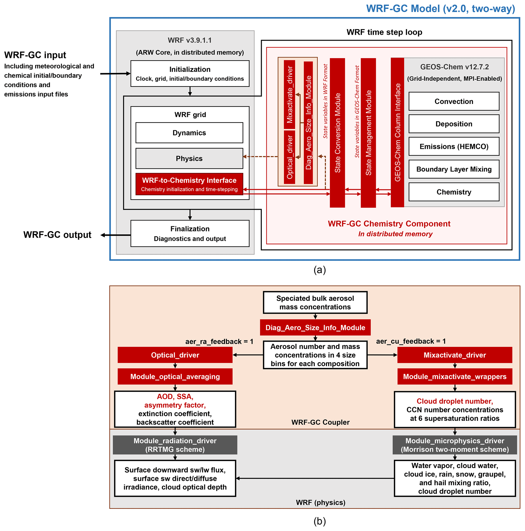
Figure 1 (a) Architectural overview of the WRF-GC coupled model (v2.0). The WRF-GC coupler (all parts shown in red) includes interfaces to the two parent models, as well as the two-way coupling modules (shown in orange). The parent models (shown in gray) are standard codes downloaded from their sources, without any modifications. (b) Flow diagram of the aerosol–radiation and aerosol–cloud interactions in the WRF-GC coupled model (v2.0).

A WRF-GC simulation is initialized and managed by WRF, which sets the global clock, dynamical and chemical time steps, domain, horizontal resolution, and vertical coordinates, as well as initial/boundary conditions. In particular, the 3-D grid system is determined by WRF and is fully adopted by the GEOS-Chem chemical module in units of atmospheric columns. At each dynamical time step, WRF performs dynamical and physical calculations. WRF calculates the grid-scale advection of meteorological variables and chemical species using the same transport scheme (Wicker and Skamarock, 2002), on the same grid system, and at the same time steps, ensuring mass conservation of the chemical species. At each chemical time step, the meteorological and chemical information is passed from WRF to GEOS-Chem through the WRF-GC coupler. Then, the GEOS-Chem column model is called to perform convective mixing, dry deposition, emissions, planetary boundary-layer mixing, gas and aerosol chemistry, and wet scavenging (except advection), in this order, within each atmospheric column at WRF-specified horizontal locations (Lin et al., 2020). Chemical information is then passed back to WRF for the next time step. At the end of the simulation, WRF finalizes the simulation and outputs the meteorological and chemical outcomes. In WRF-GC v1.0, the only chemistry-relevant operation performed by WRF is the grid-scale advection of chemical species; the chemical species do not otherwise interact with the WRF model.

In WRF-GC v2.0, we implement ARI and ACI in the two-way WRF-GC coupler. Figure 1a shows the two-way WRF-GC coupler, which extends the capabilities of the one-way coupler by the addition of three modules: (1) the Diag_Aero_Size_Info_Module, (2) the optical_driver, and (3) the mixactivate_driver. These three modules diagnose the aerosol information from GEOS-Chem for the radiative transfer and cloud microphysics calculations in WRF. Figure 1b shows the workflow of the three new modules in WRF-GC v2.0. Users can switch on ARI or ACI by specifying aer_ra_feedback=1 or aer_cu_feedback=1, respectively, in the WRF-GC configuration file (namelist.input). If ARI and ACI are both turned off, WRF-GC v2.0 will default to the one-way coupled simulation.

When users turn on the ARI, ACI, or both, the three new modules are called by the WRF-to-chemistry interface (chem_driver) at the end of each chemical time step. The Diag_Aero_Size_Info_Module diagnoses the bulk aerosol mass information from GEOS-Chem (Sect. 2.2.1) and converts it into the sectional aerosol mass and number concentrations in specified size bins using prescribed size distributions (Sect. 3.1). The sectional aerosol information is then used by the optical_driver (Sect. 3.3) and by the mixactivate_driver (Sect. 3.4) to calculate the aerosol and cloud optical properties and the activated cloud droplet number concentrations, respectively. The prognostic aerosol and cloud information is then passed to the WRF model to be used by the radiative transfer (module_radiation_driver) and cloud microphysics (module_microphysics_driver) calculations at the next time step. The diagnostic variables of aerosol mass and number concentrations are added into the WRF-GC registry file (registry.chem). Users can specify which variables to output in the registry file, and WRF will build the output arrays when WRF-GC is compiled. Below, we describe the details of the WRF and GEOS-Chem models pertinent to the two-way coupling. Further details on the two-way WRF-GC coupler calculations are given in Sect. 3.

2.2 Parent models

2.2.1 The GEOS-Chem model

WRF-GC v2.0 currently uses GEOS-Chem v12.7.2 (https://doi.org/10.5281/zenodo.3701669, The International GEOS-Chem Community, 2020) as its chemical module, but users are also able to update to the latest standard version of GEOS-Chem through the existing WRF-GC architecture. The chemical processes in GEOS-Chem v12.7.2 are mostly the same as those in GEOS-Chem v12.2.1, which is used in WRF-GC v1.0 and described in detail in Lin et al. (2020). The standard chemical mechanism in GEOS-Chem v12.7.2 includes a comprehensive O_x–NO_x–VOC–halogen–aerosol chemical mechanism in the troposphere and uses the unified tropospheric–stratospheric chemistry extension (UCX) for stratospheric chemistry (Eastham et al., 2014). One of the critical updates in GEOS-Chem v12.7.2 is the reduced sensitivity of surface resistance to temperature (Jaeglé et al., 2018). Also, the bulk surface resistance of nitric acid is updated to 1 s cm⁻¹ to reflect its high affinity for natural surfaces. These updates increase the dry deposition velocities of the nitric acid and nitrate, thereby correcting previous overestimation of surface nitrate concentrations, especially in winter (Jaeglé et al., 2018).

Table 1 Aerosol types in WRF-GC and their prescribed properties and size distributions.

Aerosol species in the standard GEOS-Chem chemical mechanism include primary dust, sea salt, primary organic carbon aerosol (POC), primary black carbon aerosol (BC), secondary inorganic aerosols (sulfate, nitrate, ammonium), and secondary organic aerosols (SOAs) (Table 1). Sea salt aerosol masses in GEOS-Chem are simulated in two size ranges: the accumulation mode (dry radii between 0.1 and 0.5 µm) and the coarse mode (dry radii between 0.5 and 4 µm) (Jaeglé et al., 2011). Dust aerosol masses are simulated in four size ranges, with effective radii of 0.7, 1.4, 2.4, and 4.5 µm, respectively (Fairlie et al., 2007). All other aerosol species are simulated by their individual bulk masses, assuming static log-normal dry size distributions for each species (Martin et al., 2003; Drury et al., 2010; Jaeglé et al., 2011). Secondary inorganic aerosols are simulated with the ISORROPIA II algorithm (Fountoukis and Nenes, 2007). Freshly emitted POC and BC aerosols are assumed to be 50 % hydrophobic and 50 % hydrophilic, with a 1.2 d conversion timescale from hydrophobic to hydrophilic (Q. Wang et al., 2014). Primary organic aerosol masses are estimated from POC mass using either a default global organic aerosol to organic carbon (OA $/$ OC) mass ratio of 2.1 or spatiotemporally varying OA $/$ OC ratios (Philip et al., 2014). GEOS-Chem provides two options for simulating the formation of SOA. By default, GEOS-Chem uses the “simple SOA” scheme: biogenic isoprene and monoterpene, as well as CO emitted from anthropogenic and biomass burning sources, are taken as proxy precursors to irreversibly form SOA at specified mass yields on a 1 d timescale (Kim et al., 2015; Pai et al., 2020). This scheme simulates relatively accurate amounts of SOA without detailed chemical calculations (Miao et al., 2020). Alternatively, GEOS-Chem can also use a volatility basis set (VBS) scheme (Robinson et al., 2007; Pye et al., 2010) to calculate complex SOA formation from the oxidation of monoterpenes, sesquiterpenes, and light aromatics. The complex SOA scheme also includes SOA formed via the aqueous-phase reactions of oxidation products from isoprene (Marais et al., 2016). GEOS-Chem assumes static, log-normal dry size distributions for its simulated bulk aerosol species (except dust), as well as prescribed aerosol hygroscopicity and optical properties at multiple wavelengths under different relative humidity, for photolysis and heterogeneous chemistry calculations (Köpke et al., 1997; Martin et al., 2003; Drury et al., 2010; Jaeglé et al., 2011; Latimer and Martin, 2019).

In this work, we developed the two-way WRF-GC coupler based on the standard bulk-mass representation of aerosol and the simple SOA scheme, involving the 14 aerosol types shown in Table 1. The goal is to include the ARI and ACI in WRF-GC while maintaining high computational efficiency. GEOS-Chem offers two optional schemes for size-resolved aerosol simulations: the Advanced Particle Microphysics (APM) scheme (Yu and Luo, 2009) and the TwO-Moment Aerosol Sectional (TOMAS) microphysics packages (Kodros and Pierce, 2017). These schemes more accurately simulate size-dependent aerosol chemistry and microphysics, albeit at higher computational costs, but they are not yet supported by the GEOS-Chem column interface. Our developed WRF-GC coupler with ARI and ACI can be extended to the APM and TOMAS schemes in the future, once those two schemes become compatible with the GEOS-Chem column interface.

2.2.2 The WRF model

WRF-GC v2.0 currently uses the WRF model (v3.9.1.1) to perform online calculations of meteorological processes, advection of chemical species, cloud microphysics, and radiative transfer with aerosol effects. WRF is a mesoscale numerical weather model for research and operational applications (Skamarock et al., 2008, 2019). WRF simulates atmospheric dynamics by solving fully compressible, Eulerian non-hydrostatic equations on either hybrid sigma–eta (default) or terrain-following vertical coordinates. WRF uses the staggered Arakawa C-horizontal grids at resolutions of 100 to 1 km and supports Lambert-conformal, Mercator, latitude–longitude, and polar stereographic projections. WRF offers multiple parameterization options for cloud microphysics, cumulus parameterization, planetary boundary layer physics, shortwave/longwave radiative transfer, and land surface physics (Skamarock et al., 2019). The options currently supported in WRF-GC are listed in Lin et al. (2020).

Only a few radiative transfer and microphysics schemes in WRF are currently coupled to prognostic aerosol information, and WRF-GC v2.0 supports these existing schemes. However, our treatments of aerosol information in the two-way WRF-GC coupler are abstracted and generalized, such that the coupler may be extended to support other radiative and microphysical schemes in WRF in the future. Most mesoscale simulations of ACI consider only the feedback of aerosols to large-scale microphysics but do not explicitly simulate the impacts of aerosol on subgrid convective clouds (e.g., Wu et al., 2011; Zhao et al., 2017). Also, most of the cumulus parameterization schemes in the standard WRF model (v3.9.1.1) do not respond explicitly to prognostic aerosol information. The only exception is the Grell–Freitas ensemble scheme (Grell and Freitas, 2014), which parameterizes the conversion of cloud water to rain water as a function of prognostic cloud condensation nuclei (CCN) number. The Grell–Freitas ensemble scheme will be supported in a future version of WRF-GC.

In WRF, two shortwave radiation schemes are coupled to prognostic aerosol information: the Rapid Radiative Transfer Model for Global Circulation Model (RRTMG) shortwave radiation scheme (Iacono et al., 2008) and the Goddard shortwave radiation scheme (Chou and Suarez, 1994). The RRTMG shortwave radiation scheme includes atmospheric Rayleigh scattering, molecular absorption by water vapor, ozone, oxygen, carbon dioxide, and methane, as well as the radiative extinction by clouds and aerosols in 14 spectral bands between 0.2 and 12.2 µm. The Goddard shortwave radiation scheme includes 11 spectral bands between 0.175 and 10 µm. It calculates atmospheric Rayleigh scattering, absorption by water vapor, ozone, oxygen, and carbon dioxide, as well as scattering and absorption by clouds and aerosols. For longwave radiation, only the RRTMG scheme (Iacono et al., 2008) has been coupled to prognostic aerosol information. The RRTMG longwave radiation scheme accounts for the absorption by water vapor, carbon dioxide, ozone, methane, oxygen, nitrous oxide, nitrogen, and several halocarbons, as well as cloud and aerosols.

When ARI is turned on (aer_ra_feedback=1 in namelist.input), WRF will ingest prognostic bulk aerosol optical information from the interface with the chemistry module. WRF further interpolates the aerosol optical properties to the specific wavelengths compatible with the shortwave radiation schemes. The aerosol optical depth (AOD) is interpolated or extrapolated using the Ångström exponent method (Eck et al., 1999), while the single scattering albedo (SSA) and the asymmetry factor are linearly interpolated. If ARI is turned off (aer_ra_feedback=0 in namelist.input), the radiative schemes ignore the aerosol effects on radiation (aer_opt=0 in namelist.input), use climatological aerosol data from Tegen et al. (1997) (aer_opt=1), or use the user-defined aerosol optical properties (aer_opt=2) specified in the WRF-GC configuration file (namelist.input).

For ACI, only two cloud microphysical schemes in the WRF model are coupled to prognostic aerosol information: the Lin et al. scheme (Lin et al., 1983; Chen and Sun, 2002) and the Morrison two-moment scheme (Morrison et al., 2009). WRF uses an aerosol activation scheme developed by Abdul-Razzak and Ghan (2000, 2002). When ACI is turned on (progn=1 and naer=ignored in namelist.input), the interface to the chemical module will call the aerosol activation scheme to diagnose the activated cloud droplet number in a time step. This calculation is based on a maximum supersaturation determined by the mass concentrations, number densities, and hygroscopic properties of aerosols, as well as the local air temperature and updraft velocity. Also, the radiation module in WRF uses the prognostic liquid cloud effective radii to compute the liquid cloud optical depths (LCODs). If ACI is turned off, WRF either diagnoses the activated cloud droplet number using a prescribed aerosol number and size distribution (progn=1 and naer=specified) or uses a constant source of activated cloud droplets (100 cm⁻³ per time step in the Lin et al. scheme and 250 cm⁻³ per time step in the Morrison two-moment scheme) (progn=0). In the event where WRF does use a constant source of activated cloud droplets, the predicted cloud droplet number will effectively be around that prescribed number. Also, if ACI is turned off, WRF uses prescribed constant values of liquid cloud effective radii to calculate LCODs.

3 New developments in WRF-GC v2.0

Here, we describe the detailed diagnostics performed in the two-way WRF-GC coupler to communicate aerosol and cloud information between GEOS-Chem and WRF. Some of our diagnostics are developed by imitating the connections between WRF and the chemical module in the WRF-Chem model (Grell et al., 2005; Fast et al., 2006; Chapman et al., 2009). We also describe the software engineering developments that enable nested-domain simulations in WRF-GC v2.0.

3.1 Diagnosing the size and number of dry aerosols

The size distribution of aerosol is a critical property that affects its optical effects and its ability to be activated into CCN. We develop the Diag_Aero_Size_Info_Module to diagnose the sectional size distribution of aerosol mass and number concentrations from the bulk aerosol masses simulated by GEOS-Chem. For each of the aerosol types (except dust) in GEOS-Chem, we distribute the aerosol dry masses into four effective dry diameter bins used by WRF-GC. We assume the aerosol within each size bin to be internally mixed. The lower and upper dry diameter bounds of the four bins (Table 2) are from the Model for Simulating Aerosol Interactions and Chemistry (MOSAIC) four-bin sectional parameterization (Zaveri et al., 2008). With the exception of dust, we assume that the number density of aerosol type i follows a log-normal distribution (Eq. 1):

$$\begin{array}{}\text{(1)}& \begin{array}{rl}{n}_i\left(\ln D_i\right)& ={\displaystyle \frac{\mathrm{d}N}{\mathrm{d}\ln D_i}}\\ & ={\displaystyle \frac{N}{\sqrt{\mathrm{2}\mathit{\pi }}\ln {\mathit{\sigma }}_i}}\exp \left[-{\displaystyle \frac{{\left(\ln D_i-\ln D_{\mathrm{g},i}\right)}^{\mathrm{2}}}{\mathrm{2}{\ln }^{\mathrm{2}}{\mathit{\sigma }}_i}}\right],\end{array}\end{array}$$

where D_i is the particle dry diameter, and N is the total number concentration of the internally mixed particles. n_i(ln D_i) is the number concentration density as a function of ln D_i. D_g,i and σ_i are the effective geometric mean dry diameter and the effective geometric standard deviation of the log-normal distribution, respectively (Table 1). Thus, the mass concentration density of the ith aerosol type (m_i(ln D_i)) can be expressed using D_i, n_i(ln D_i), and the density of aerosol type i (ρ_i), as shown in Eq. (2):

$$\begin{array}{}\text{(2)}& \begin{array}{rl}{m}_i\left(\ln D_i\right)& ={\mathit{\rho }}_i\cdot {\displaystyle \frac{\mathit{\pi }{D}_i^{\mathrm{3}}}{\mathrm{6}}}\cdot n_i\left(\ln D_i\right)\\ & ={\mathit{\rho }}_i\cdot {\displaystyle \frac{\mathit{\pi }{D}_i^{\mathrm{3}}}{\mathrm{6}}}\\ & \cdot {\displaystyle \frac{N}{\sqrt{\mathrm{2}\mathit{\pi }}\ln {\mathit{\sigma }}_i}}\exp \left[-{\displaystyle \frac{{\left(\ln D_i-\ln D_{\mathrm{g},i}\right)}^{\mathrm{2}}}{\mathrm{2}{\ln }^{\mathrm{2}}{\mathit{\sigma }}_i}}\right].\end{array}\end{array}$$

Table 2 Upper and lower bounds of particle dry diameter for the four aerosol size bins used by WRF-GC.

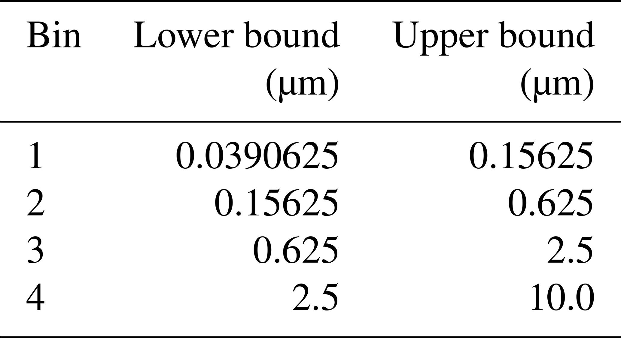
Table 1 summarizes the prescribed values of D_g,i, σ_i, and ρ_i for each aerosol type used in our two-way WRF-GC coupler. The D_g,i and σ_i for secondary inorganic aerosols, BC, POC, and sea salt in accumulation and coarse modes are identical to the values used in the GEOS-Chem model for photolysis and heterogeneous chemistry calculations (Martin et al., 2003; Drury et al., 2010; Jaeglé et al., 2011). We assume that the log-normal distribution of SOA is identical to that of POC. The dry mass of aerosol type i (except dust) in each of WRF-GC's four size bins can be calculated as Eq. (3):

$$\begin{array}{}\text{(3)}& M_{i,j}=M_i\cdot {\displaystyle \frac{{\int }_{l_{\mathrm{W},j}}^{h_{\mathrm{W},j}}{m}_i\left(\ln D_i\right)\mathrm{d}\ln D_i}{{\int }_{\mathrm{0}}^{\mathrm{\infty }}{m}_i\left(\ln D_i\right)\mathrm{d}\ln D_i}},\end{array}$$

where l_W,j and h_W,j are the lower and upper dry diameter bounds of the jth size bin. M_i,j is the mass of aerosol type i in the jth bin, and M_i is the total mass of aerosol type i. The total number concentration of the internally mixed aerosol population (N) cancels out in Eq. (3).

GEOS-Chem simulates dust mass concentrations in four internal size bins, which need to be redistributed into the four size bins used by WRF and WRF-GC (shown in Table 2). To achieve this, we mimic the redistribution scheme of dust aerosols in the Goddard Chemistry Aerosol Radiation Transport model (GOCART, Chin et al., 2002), in which the first four internal size bins are identical to those used in GEOS-Chem. In Eqs. (4) and (5), the l and h with the subscripts W and G represent the lower and upper dry diameter bounds of each size bin used in WRF-GC and GEOS-Chem, respectively. The indices j and k refer to the size bins used by WRF-GC and GEOS-Chem, respectively ($j,k\in [\mathrm{1},\mathrm{4}]$). Equation (4) calculates the fraction of dust mass within the GEOS-Chem size bin k that is mapped to the WRF-GC size bin j. The mass is distributed by the logarithmic of particle diameter. diag_dst(j), the total dust mass concentrations within the WRF-GC size bin j, is the sum of the dust mass mapped into that bin from the four GEOS-Chem dust size bins (Eq. 5).

$$\begin{array}{}\text{(4)}& {\displaystyle }\mathrm{dstfrac}(j,k)={\displaystyle \frac{\begin{array}{c}max\left[\mathrm{0},min\left[\ln h_{\mathrm{W}}\left(j\right),\ln h_{\mathrm{G}}\left(k\right)\right]\right.\\ \left.-max\left[\ln l_{\mathrm{W}}\left(j\right),\ln l_{\mathrm{G}}\left(k\right)\right]\right]\end{array}}{\ln h_{\mathrm{G}}\left(k\right)-\ln l_{\mathrm{G}}\left(k\right)}}\text{(5)}& {\displaystyle }\mathrm{diag}\mathrm{\_}\mathrm{dst}\left(j\right)=\sum _{k=\mathrm{1}}^{\mathrm{4}}\mathrm{dst}\left(k\right)\cdot \mathrm{dstfrac}(j,k)j,k\in [\mathrm{1},\mathrm{4}]\end{array}$$

Equation (6) diagnoses the number concentrations of the internally mixed aerosols in each size bin. The total dry aerosol volume in the jth size bin (${\sum }_{i=\mathrm{1}}^{\mathrm{10}}{V}_{\mathrm{d},i,j}$) is calculated by summing the dry aerosol volume of the 10 aerosol types. The aerosol number concentrations in the jth size bin, N_j, can then be diagnosed by dividing the total dry aerosol volume in that size bin by the mean particle size:

$$\begin{array}{}\text{(6)}& N_j={\displaystyle \frac{\mathrm{6}}{\mathit{\pi }{\left[\frac{\mathrm{1}}{\mathrm{2}}\left(l_{\mathrm{W}}\left(j\right)+h_{\mathrm{W}}\left(j\right)\right)\right]}^{\mathrm{3}}}}\cdot \sum _{i=\mathrm{1}}^{\mathrm{10}}{V}_{\mathrm{d},i,j}.\end{array}$$

3.2 Diagnosing water uptake of aerosols

The hygroscopic growth of aerosols at ambient relative humidity impacts their wet radii and optical properties. We follow the method developed by Petters and Kreidenweis (2007, 2013) to diagnose the uptake of water by aerosols and the resulting wet radii. According to the Zdanovskii–Stokes–Robinson (ZSR) assumption (Stokes and Robinson, 1966), the total aerosol liquid water is equal to the sum of the water taken up by each aerosol constituent:

$$\begin{array}{}\text{(7)}& V_{\mathrm{w},j}={\displaystyle \frac{a_{\mathrm{w}}}{\mathrm{1}-a_{\mathrm{w}}}}\sum _{i=\mathrm{1}}^{\mathrm{10}}{\mathit{\kappa }}_i{V}_{\mathrm{d},i,j}.\end{array}$$

V_w,j is the total volume of aerosol liquid water in the jth size bin. a_w is the water activity, equal to the fractional relative humidity. κ_i is the hygroscopicity of the aerosol type i (Table 1). The wet radius of the internally mixed aerosols in the jth size bin, R_w,j, is required for the calculation of aerosol optical properties and are calculated by Eq. (8):

$$\begin{array}{}\text{(8)}& R_{\mathrm{w},j}={\displaystyle \frac{\mathrm{1}}{\mathrm{2}}}{\left({\displaystyle \frac{\mathrm{6}}{\mathit{\pi }}}\cdot {\displaystyle \frac{V_{\mathrm{w},j}+{\sum }_{i=\mathrm{1}}^{\mathrm{10}}{V}_{\mathrm{d},i,j}}{N_j}}\right)}^{\frac{\mathrm{1}}{\mathrm{3}}}.\end{array}$$

3.3 Aerosol–radiation interactions

When ARI is turned on in WRF-GC v2.0, the new optical_driver module calls the module_optical_averaging to diagnose the bulk optical properties of the internally mixed aerosols at each model grid and pass them to WRF for radiative transfer calculations. The diagnosed bulk optical properties include the AOD, the SSA, and the asymmetry factor at four specific wavelengths (300, 400, 600, 999 nm) for shortwave radiative transfer and the AOD at 16 specific wavelengths for longwave radiative transfer. Our module_optical_averaging is developed by modifying a similar module from WRF-Chem (Fast et al., 2006). The module_optical_averaging module ingests the wet radius (R_w,j) and the number concentration (N_j) of aerosol particles in the jth size bin. The bulk refractive indices for the internally mixed aerosols in each size bin are calculated by volume weighting the refractive indices for individual aerosol species using a look-up table (Barnard et al., 2010). The tabulated refractive indices for water, sulfate, dust, sea salt, and primary and secondary OC are wavelength dependent, while the refractive indices for other aerosol species do not vary with wavelength. The module then uses the bulk refractive indices to calculate the bulk extinction efficiency (Q_e), the bulk scattering efficiency (Q_s), and the intermediate asymmetry factor (g^′) for the internally mixed aerosols as a function of the size parameter α_j $\left(=\frac{\mathrm{2}\mathit{\pi }{R}_{\mathrm{w},j}}{\mathit{\lambda }}\right)$ based on Mie theory (Wiscombe, 1979). We use a Chebyshev economization (Press et al., 1992) to avoid the full Mie calculation at each time step following Fast et al. (2006). A full Mie calculation is only performed at the first chemical time step to obtain the Chebyshev expansion coefficients for each complex refractive index.

The bulk total extinction coefficient (b_ext) at wavelength λ is calculated as the sum of extinction by aerosols in all four size bins (Eq. 9):

$$\begin{array}{}\text{(9)}& b_{\mathrm{ext}}\left(\mathit{\lambda }\right)=\sum _{j=\mathrm{1}}^{\mathrm{4}}{Q}_{\mathrm{e}}\left({\mathit{\alpha }}_j\right)\cdot \mathit{\pi }{R}_{\mathrm{w},j}^{\mathrm{2}}\cdot N_j.\end{array}$$

The bulk AOD in a layer of atmosphere of dz thickness is (Eq. 10)

$$\begin{array}{}\text{(10)}& \mathit{\tau }\left(\mathit{\lambda }\right)=b_{\mathrm{ext}}\left(\mathit{\lambda }\right)\cdot \mathrm{d}z.\end{array}$$

The single scattering albedo (ϖ₀), which represents the scattered percentage in the total light extinction of aerosol particles, is calculated as (Eq. 11)

$$\begin{array}{}\text{(11)}& {\mathit{\varpi }}_{\mathrm{0}}\left(\mathit{\lambda }\right)={\displaystyle \frac{b_{\mathrm{s}}\left(\mathit{\lambda }\right)}{b_{\mathrm{ext}}\left(\mathit{\lambda }\right)}},\end{array}$$

where b_s is the scattering coefficient of aerosols, given by (Eq. 12)

$$\begin{array}{}\text{(12)}& b_{\mathrm{s}}\left(\mathit{\lambda }\right)=\sum _{j=\mathrm{1}}^{\mathrm{4}}{Q}_{\mathrm{s}}\left({\mathit{\alpha }}_j\right)\cdot \mathit{\pi }{R}_{\mathrm{w},j}^{\mathrm{2}}\cdot N_j.\end{array}$$

The bulk asymmetry factor, g, represents the asymmetry between the forward scattering and backward scattering of aerosol particles:

$$\begin{array}{}\text{(13)}& g\left(\mathit{\lambda }\right)={\displaystyle \frac{\sum _{j=\mathrm{1}}^{\mathrm{4}}{Q}_{\mathrm{s}}\left({\mathit{\alpha }}_j\right)\cdot \mathit{\pi }{R}_{\mathrm{w},j}^{\mathrm{2}}\cdot N_j\cdot g^{\prime }\left({\mathit{\alpha }}_j\right)}{b_{\mathrm{s}}\left(\mathit{\lambda }\right)}},\end{array}$$

where g^′ is the intermediate asymmetry factor related to the size parameter α_j.

3.4 Aerosol–cloud interactions

We couple the activation of aerosol particles to the Morrison two-moment scheme (Morrison et al., 2009) and the Lin et al. scheme (Lin et al., 1983; Chen and Sun, 2002) in WRF-GC. To achieve this, we develop an interface routine wrfgc_mixactivate (contained in module_mixactivate_wrappers in the coupler) by mimicking a similar routine in WRF-Chem. Equation (14) shows the rate of change of the cloud droplet number concentration (N_c) within a WRF model grid in the two cloud microphysical schemes. The rate of change of N_c is determined by the advection of cloud droplet number ($-\mathit{V}\cdot \mathrm{\nabla }{N}_{\mathrm{c}}$), the vertical transport of cloud droplet number (D), the loss rate of cloud droplet number due to collision, coalescence, and collection (C), and the evaporation of cloud droplets (E), as well as the rate of cloud droplet activation (S).

$$\begin{array}{}\text{(14)}& {\displaystyle \frac{\partial N_{\mathrm{c}}}{\partial t}}=-\left(\mathit{V}\cdot \mathrm{\nabla }{N}_{\mathrm{c}}\right)+D-C-E+S\end{array}$$

When ACI is turned on (aer_cu_feedback=1 and progn=1) in WRF-GC, the mixactivate_driver module in the WRF-GC coupler calls the existing WRF subroutine mixactivate through an interface routine (wrfgc_mixactivate) to calculate the number of aerosol particles activated into cloud droplets (S) and pass it to WRF. wrfgc_mixactivate first calculates the volume-weighted bulk hygroscopicity using the diagnostic aerosol mass and number within each aerosol size bin and then calls the subroutine mixactivate. The subroutine mixactivate uses the Köhler theory to calculate the activated aerosol mass and number when the ambient supersaturation is over the critical supersaturation of aerosols (Abdul-Razzak and Ghan, 2000, 2002). The total aerosol mass and number concentrations are treated as two explicit population: interstitial and cloud borne. The prognostic aerosol mass and number concentrations are initialized as interstitial before passing to the mixactivate_driver module. The activated aerosols will be then considered cloud borne, while the unactivated aerosols remain interstitial. The mixactivate subroutine also calculates CCN at six specified supersaturation ratios (0.02 %, 0.05 %, 0.1 %, 0.2 %, 0.5 %, and 1 %) as output diagnostics.

3.5 Development of nested-grid functionality and online lightning NO_x emissions

We implement the nested-domain functionality into WRF-GC v2.0 to enable meteorology–chemistry simulations at higher resolution. In WRF-GC v1.0 (Lin et al., 2020), the coupling between WRF and GEOS-Chem was limited to a single domain of arbitrary dimension and resolution. This was because the modules in previous GEOS-Chem versions (prior to v12.4.0) used a single memory space for the entire simulation, such that the domain dimensions in GEOS-Chem were fixed once the simulation was initialized.

We improve the state management module in WRF-GC v2.0 to better control the memory space of GEOS-Chem. Figure 2 illustrates the operation of the state management module when running WRF-GC v2.0 in a nested-domain configuration. When running a nested-domain simulation, WRF designates separate memory space for each domain, and at each time step WRF alternately accesses the memory spaces for each domain. To achieve the same functionality in GEOS-Chem, we modify the GEOS-Chem model (implemented in the standard code for v12.4.0 and after) so that all of its internal variables are saved into state objects (meteorology, chemistry, and diagnostic state variables), which are labeled for the specific simulation domain. We then modify the state management module, such that at each time step during runtime, the state management module will determine the GEOS-Chem domain being processed, access the corresponding state objects, and provide them to GEOS-Chem. The emission module of GEOS-Chem, the Harmonized Emissions Component (HEMCO), has also been updated to fully objectify its memory space (Keller et al., 2014; Lin et al., 2021). This allows WRF-GC v2.0 to execute separate copies of HEMCO for each of the nested domains.

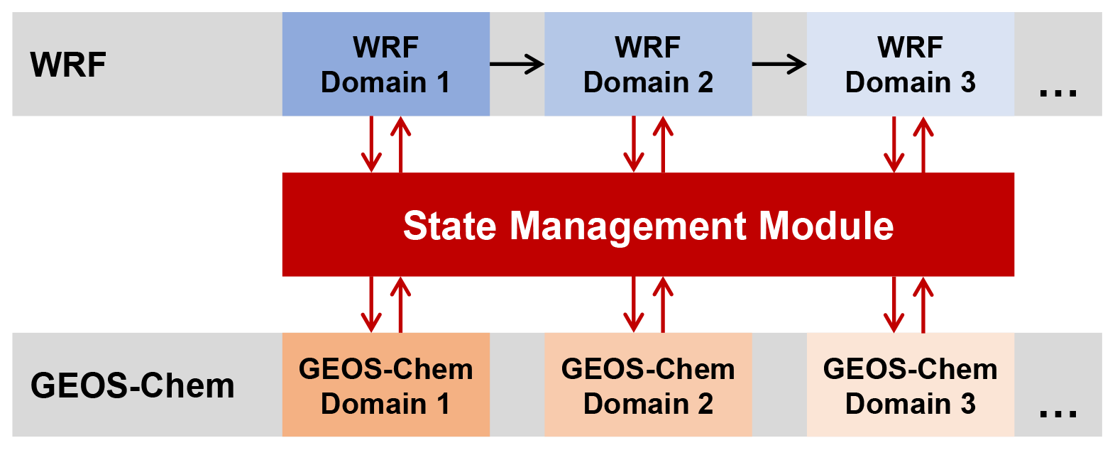
Figure 2 Illustration of the WRF-GC state management module operating in a nested-domain configuration.

WRF-GC v2.0 allows both one-way and two-way information exchange between the nested domains, supported by the WRF framework. In a nested-domain simulation, the outer (coarser) domain will always provide lateral boundary conditions to its immediate inner (finer) domain (one-way information exchange). Users may also turn on the two-way information exchange option (feedback=1 in the WRF-GC namelist), which further allows information at the boundaries of the inner domain to be averaged and fed back to the immediate outer domain at every time step.

In addition to the meteorology-dependent emissions in WRF-GC v1.0 (Lin et al., 2020), in WRF-GC v2.0 we further couple WRF meteorology to the online lightning NO_x emission scheme in the HEMCO module (Murray et al., 2012). Intra-cloud and cloud-to-ground flash densities are functions of the cloud-top height and are calculated by the lightning parameterization in WRF (Price and Rind, 1992; Wong et al., 2013). HEMCO then calculates lightning NO_x emissions using the prescribed NO_x production rates (500 moles per flash for latitudes northward of 35^∘ N; 260 moles per flash elsewhere) (Murray et al., 2012) and vertically distributes them from the surface to the local convective cloud-top level (Ott et al., 2010).

3.6 Computational performance of WRF-GC v2.0

We conduct 2 d (27 to 29 June 2019) simulations using the WRF-GC (v2.0) model and the GEOS-Chem Classic nested-grid model (v12.7.2) to compare their computational performance. Simulations with both models are configured with 245 × 181 atmospheric columns over China. The WRF-GC simulations have 50 vertical levels, while the GEOS-Chem Classic nested-grid simulation has 47 vertical levels. The WRF-GC model simulates meteorology online (2 min dynamical time step), while the GEOS-Chem Classic nested-grid simulation reads archived GEOS-FP assimilated meteorological dataset (https://gmao.gsfc.nasa.gov/GMAO_products/, last access: 20 June 2021) and calculates advection at 5 min time step. All simulations use the same emissions, the same chemical module (GEOS-Chem column model), and identical chemical time steps. All simulations are performed on the same single-node hardware with 24 Intel Cascade Lake physical cores, 100 GB of RAM, and a networked Lustre high-performance file system. WRF-GC uses Message Passing Interface (MPI) parallelization, while GEOS-Chem Classic uses OpenMP parallelization.

Table 3 Wall times of simulations conducted with the WRF-GC v2.0 model and the GEOS-Chem Classic nested-grid model (unit: s).

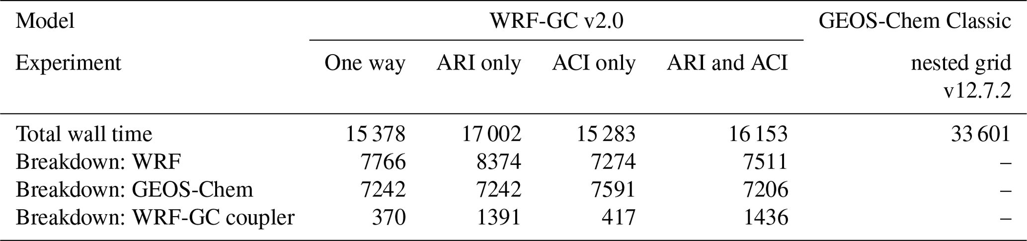
Table 3 compares the simulation wall times for the WRF-GC v2.0 model (with various chemical feedback options) and for the GEOS-Chem Classic nested-grid model. Similar to our previous diagnosis (Lin et al., 2020), a one-way WRF-GC simulation (15 282 s) is 53 % faster than a similarly configured GEOS-Chem Classic nested-grid simulation (33 601 s). The better computational performance of WRF-GC is due to its faster dynamic calculations and its more efficient parallelization of the chemical processes (Lin et al., 2020). The wall times for the two-way WRF-GC simulations with various combinations of chemical feedbacks (ARI only, ACI only, and both ARI and ACI) are all less than 11 % higher than the wall time for the one-way simulation. As expected, the slightly longer wall times in simulations with chemical feedbacks are mostly associated with the extra calculations within the WRF-GC coupler. The ARI calculations incur more wall time increases than the ACI calculations do. For reasons yet unclear, the wall time for the simulation with ARI only (17 002 s) is slightly longer than that for the simulation with both ARI and ACI (16 153 s). Nevertheless, in all WRF-GC simulations, the coupling calculations are computationally economical and consume less than 9 % of the total wall times.

4 Validation of WRF-GC simulations of regional meteorology and surface pollutant concentrations over China

4.1 Setup of model experiments

We next evaluate WRF-GC's performance in simulating regional meteorology and surface pollutant concentrations. We conduct two control simulations with full aerosol–cloud–radiation interactions using WRF-GC v2.0: one during January 2015 (Case ACRw) and one during July 2016 (Case ACRs). Table 4 summarizes the setup of our simulations. Figure 3 shows our simulation domain over East Asia, set by a Mercator projection at 27 km × 27 km spatial resolution. There are 50 vertical layers extending from the surface to 10 hPa. Case ACRw simulates 4 to 29 January 2015; Case ACRs simulates 27 June to 31 July 2016. The first four days of each simulation initialize the model. Meteorological initial conditions and boundary conditions (ICs/BCs) are taken from the National Centers for Environmental Prediction (NCEP) Final (FNL) dataset (https://doi.org/10.5065/D6M043C6, National Centers for Environmental Prediction et al., 2020) at 1^∘ resolution. Chemical ICs/BCs are from a GEOS-Chem global simulation at 2.5^∘ longitude × 2^∘ latitude, interpolated to WRF-GC horizontal and vertical grids. Meteorological and chemical BCs are updated every 6 h at the WRF-GC domain boundary. The WRF-GC simulations are not nudged with meteorological observations.

(Morrison et al., 2009)(Iacono et al., 2008)(Iacono et al., 2008)(Nakanishi and Niino, 2006)(Chen and Dudhia, 2001a, b)(Jimenez et al., 2012)(Tiedtke, 1989; C. Zhang et al., 2011; Zhang and Wang, 2017)(Morrison et al., 2009)(Iacono et al., 2008)(Iacono et al., 2008)(Hong et al., 2006)(Chen and Dudhia, 2001a, b)(Jimenez et al., 2012)(Tiedtke, 1989; C. Zhang et al., 2011; Zhang and Wang, 2017)

Table 4 Configurations of WRF-GC v2.0 experiments in this study.

Figure 3 Spatial distributions of the observed and simulated time-averaged AOD at 550 nm (a, c) during 8 to 28 January 2015 and (b, d) during 1 to 30 July 2016. (a, b) Visible Infrared Imaging Radiometer Suite (VIIRS) observations; (c) Case ACRw; (d) Case ACRs.

We further conduct sensitivity simulations over China for January 2015 and July 2016 with different combinations of ARI and ACI to investigate the impacts of chemical feedbacks on simulated meteorology and air quality (Table 4). The setups of these sensitivity simulations are identical to the control cases, except ARI and ACI are configured differently in each sensitivity simulation (Table 4). In Cases NO_ACRs and NO_ACRw, both ARI and ACI are turned off, i.e., one-way WRF-GC simulations with no chemical feedbacks to meteorology. Cases ARIs/ARIw and Cases ACIs/ACIw simulation include either ARI or ACI, respectively. Our simulations are conducted at a typical mesoscale resolution (27 km), with the cumulus parameterization (new Tiedtke) and the cloud microphysical scheme (Morrison two-moment) both turned on. Thus, the subgrid convective clouds do not explicitly respond to prognostic aerosol information. This setup is typical of mesoscale simulations and has been shown to produce similar aerosol sensitivities to those simulated at cloud-resolving resolutions (Wu et al., 2011).

Chinese monthly mean anthropogenic emissions are from the Multi-resolution Emission Inventory for China (MEIC; Li et al., 2014) with a resolution of 0.25^∘ for the years 2015 and 2016. Anthropogenic emissions from the rest of Asia are from M. Li et al. (2017), developed for the year 2010. Monthly mean biomass burning emissions are from the Global Emissions Database version 4 (GFED4; Randerson et al., 2018). Meteorology-dependent emissions, including the emissions of biogenic volatile organic compounds (Guenther et al., 2012), sea salt (Gong, 2003), dust (Zender et al., 2003), soil NO_x (Hudman et al., 2012), and lightning NO_x (Murray et al., 2012), are calculated online in the HEMCO module (Keller et al., 2014) in GEOS-Chem.

4.2 Observation datasets

4.2.1 Satellite retrievals of AOD, cloud optical properties, and surface downward shortwave radiation

We use satellite observations to evaluate WRF-GC's performance in simulating aerosol and cloud optical properties, and surface downward shortwave radiation. Monthly mean AOD observations are from the Deep Blue level-3 monthly aerosol products (AERDB_D3/M3_VIIRS_SNPP, version 1) from the Visible Infrared Imaging Radiometer Suite (VIIRS) instruments at 1^∘ spatial resolution (Sayer et al., 2018). Monthly LCOD observations are from the VIIRS Cloud Properties level-3 monthly 1^∘ grid products (CLDPROP_D3/M3_VIIRS_SNPP, version 1.1) (Platnick et al., 2019). Monthly surface downward shortwave radiation observations for July 2016 are from the Earth Polychromatic Imaging Camera (EPIC)-derived products over land at 0.1^∘ resolution (Hao et al., 2020). The EPIC-derived total downward shortwave radiation is consistent with the ground-based observations with a low global bias of −0.71 W m⁻² over land. For January 2015, due to the lack of EPIC-derived products, we use the monthly gridded product from the Clouds and the Earth's Radiant Energy System (CERES) edition 4.1 at 1^∘ resolution (Rutan et al., 2015). The spatiotemporal variations of the surface downward shortwave radiation observed by the EPIC and CERES instruments are generally consistent (Hao et al., 2020).

4.2.2 Ground-based AOD measurements

We evaluate the spectral AOD simulated by WRF-GC for January 2015 against the ground-based observations from the Aerosol Robotic Network (AERONET, https://aeronet.gsfc.nasa.gov/, last access: 20 June 2021) project (version 3, level 2.0 quality-assured dataset, Giles et al., 2019). Holben et al. (1998) showed that the uncertainty of AERONET AOD under cloud-free conditions was less than ±0.01 for wavelengths over 440 nm. We select four representative sites in eastern China, where there are more than 50 % valid observations of spectral AOD at three wavelengths (500, 675, and 1020 nm) during January 2015. These four sites are (1) Chinese Academy of Meteorological Sciences in Beijing (39.93^∘ N, 116.32^∘ E), (2) Xianghe (39.75^∘ N, 116.96^∘ E), (3) China University of Mining and Technology in Xuzhou (34.22^∘ N, 117.14^∘ E), and (4) Hong Kong Polytechnic University in Hong Kong (22.30^∘ N, 114.18^∘ E).

4.2.3 Surface measurements of air pollutants, air temperature, and planetary boundary layer height

Hourly surface measurements of PM_2.5 and ozone are managed by the Ministry of Ecology and Environment of China (http://www.cnemc.cn, last access: 20 June 2021). Our protocol for data quality control follows Jiang et al. (2020). We exclude sites with less than 90 % valid hourly data during January 2015 and July 2016. For comparison between observations and model results, we calculate the average PM_2.5 and ozone measurements in a WRF-GC grid. In all, we compare model results to summertime ozone observations at 562 sites and to wintertime PM_2.5 observations at 513 sites, respectively. Surface air temperature measurements over China are downloaded from the US National Climate Data Center (https://gis.ncdc.noaa.gov/maps/ncei/cdo/hourly, last access: 20 June 2021), and we exclude sites with less than 90 % valid data. In all, surface air temperature measurements at 150 and 215 sites are used to evaluate our simulations during January 2015 and July 2016, respectively. Finally, Guo et al. (2016) analyzed the rawinsonde observations over China to determine the daily planetary boundary layer heights (PBLHs) during January 2011 to July 2015. We use the observed PBLH at 120 sites at 08:00 and 20:00 local time (00:00 and 12:00 UTC, respectively) to validate the simulated PBLH in January 2015.

4.3 Validation of the simulated AOD over East Asia

Figure 3a and c compare the AOD at 550 nm wavelength over East Asia as observed by VIIRS and as simulated by WRF-GC (Case ACRw) during 8 to 28 January 2015. For comparison against VIIRS observations, we use the simulated AODs at 300 and 999 nm to calculate the Ångström exponent of the internally mixed bulk aerosol and then interpolated the simulated AOD at 400 to 550 nm. WRF-GC is generally able to reproduce the spatial distribution of AOD observed by VIIRS over eastern China (20–40^∘ N, 105–130^∘ E) with a spatial correlation coefficient of r = 0.64. WRF-GC reproduces the high AOD values over the Sichuan Basin but underestimates the AOD over other parts of eastern China. The observed and simulated AODs at 550 nm over eastern China in January 2015 are 0.37 and 0.21, respectively. WRF-GC also underestimates the AOD over the Xinjiang, Qinghai, and Gansu provinces in western China, likely reflecting an underestimation of dust.

Figure 3b and d compare the observed and simulated (Case ACRs) AOD at 550 nm during July 2016. VIIRS observes AOD values exceeding 0.6 over the North China Plain (NCP) area, reflecting the large amounts of aerosols and their hygroscopic growth over that area. The simulated spatial distribution of AOD is generally consistent with that from VIIRS, but the peak values over the NCP are lower than the observations by 50 %. We also compare model results to the AOD observations from the MODIS instrument (Platnick et al., 2017a, b) and similarly find that the simulated AODs are spatially consistent but lower than the MODIS observations over eastern China.

Figure 4 Comparison of simulated daily AOD (Case ACRw) against the AERONET daily AOD observations at 500, 675, and 1020 nm at four sites during 8 to 28 January 2015: (a) Beijing, (b) Xianghe, (c) Xuzhou, and (d) Hong Kong. Also shown are the normalized mean biases (NMBs) and the temporal correlation coefficients (r) between the simulated and observed spectral AODs.

Figure 4 compares the time series of the simulated daily spectral AOD against the AERONET observations at the four representative Chinese sites during 8 to 28 January 2015. At each site, we interpolate the simulated spectral AODs at 400, 600, and 999 nm to the AERONET observation wavelengths of 500, 675, and 1020 nm, respectively, using the Ångström exponent method (Eck et al., 1999). WRF-GC reproduces the observed day-to-day variation of AOD at these four sites during January 2015. The temporal correlation coefficients between the observed and simulated AODs at all sites and wavelengths range between 0.55 and 0.86, except for the correlation coefficient between the observed and simulated 500 nm AOD in Beijing (0.44). However, the simulated AODs are consistently lower than the AERONET AODs, especially during high AOD events.

Our analyses above show that AODs simulated by WRF-GC reproduce the spatiotemporal variability of the AODs observed by satellite and ground-based networks. However, the simulated AODs are consistently lower than these observations. Previous comparisons of AODs simulated by regional models against satellite observations also often found spatial consistency but significant low biases in the models (Gao et al., 2014; Gan et al., 2015; Xing et al., 2015; Zhang et al., 2016). Curci et al. (2015) showed that the uncertainties for the model AODs are associated with the assumed mixing state, refractive indices, and hygroscopicity of aerosols. In particular, assumptions of the aerosol mixing state can lead to 30 % to 35 % uncertainty on the simulated AOD (Fassi-Fihri et al., 1997; Curci et al., 2015). In addition, the WRF-GC model may have underestimated the abundance of aerosols over China, as indicated by the slight underestimation of surface PM_2.5 concentrations shown below (Sect. 4.6). On the other hand, several studies showed that the regional distributions of AOD observed by VIIRS and MODIS are consistent with the AERONET measurements, but both VIIRS and MODIS observations are biased high compared to AERONET observations over Asia (Wang et al., 2020). This high bias in the satellite-observed AOD may partially account for the discrepancy between the simulated and satellite AODs. The cause of the discrepancy between observed and simulated AOD should be further investigated in future studies.

4.4 Validation of the simulated LCOD and liquid cloud droplet effective radii

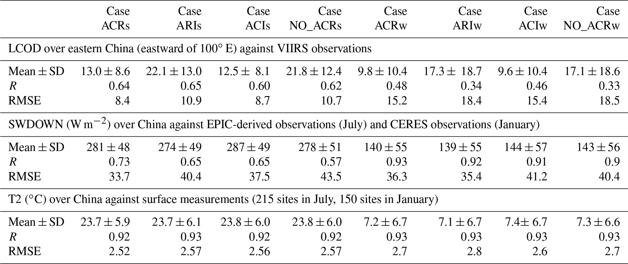
Figure 5a and b compare the July mean LCODs retrieved by VIIRS and results from the Case ACRs simulation for July 2016. The spatial distributions of observed and simulated LCOD are generally consistent over East Asia. The observed and simulated LCODs are both high over northeastern China, central-western China, and along the southern slopes of the Himalayas. The observed and simulated LCODs are relatively low over the Tibetan Plateau. The simulated domain-average LCOD from Case ACRs is 12.0 ± 8.1, lower than the domain-averaged LCOD retrieved by VIIRS (18.2 ± 7.5). The underestimation of simulated LCOD is mostly over western China and the South China Sea. Over eastern China (eastward of 100^∘ E), the simulated magnitude and spatiotemporal patterns of LCOD are in good agreement with the observations (spatial correlation coefficient of r = 0.64, normalized mean bias of −25.3 %). Figure 6a and b show the observed and simulated (Case ACRw) average LCODs during 8 to 28 January 2015. The model reproduces the spatial distribution of LCODs observed by VIIRS over China, including in particular the high LCODs over southern China. However, the simulated LCOD is considerably lower than the VIIRS LCOD observations elsewhere in the domain.

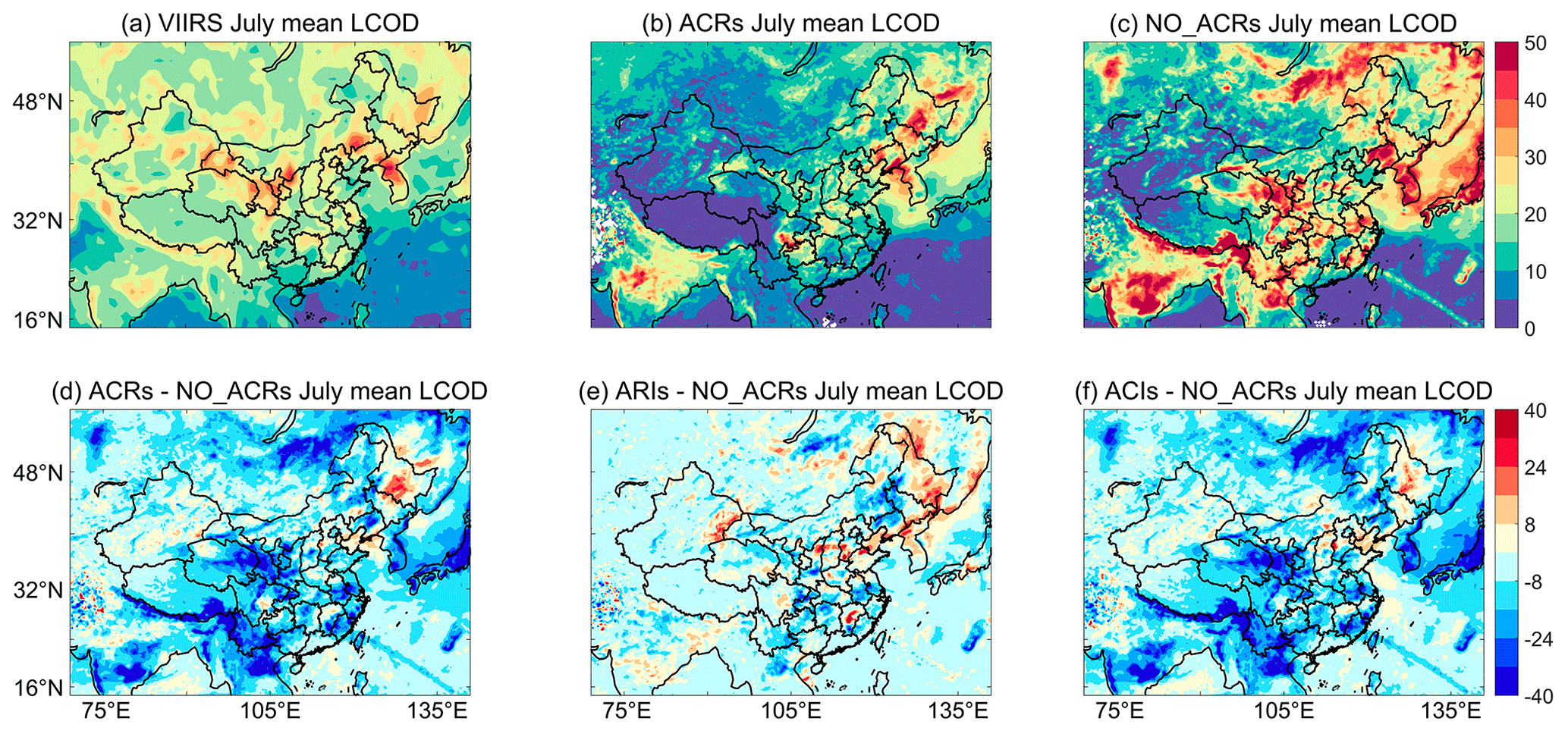
Figure 5 Monthly mean LCOD from (a) VIIRS observations, (b) the Case ACRs simulation, and (c) the Case NO_ACRs simulation during July 2016. Also shown are the differences in simulated LCOD between (d) Case ACRs and Case NO_ACRs, (e) Case ARIs and Case NO_ACRs, and (f) Case ACIs and Case NO_ACRs during July 2016.

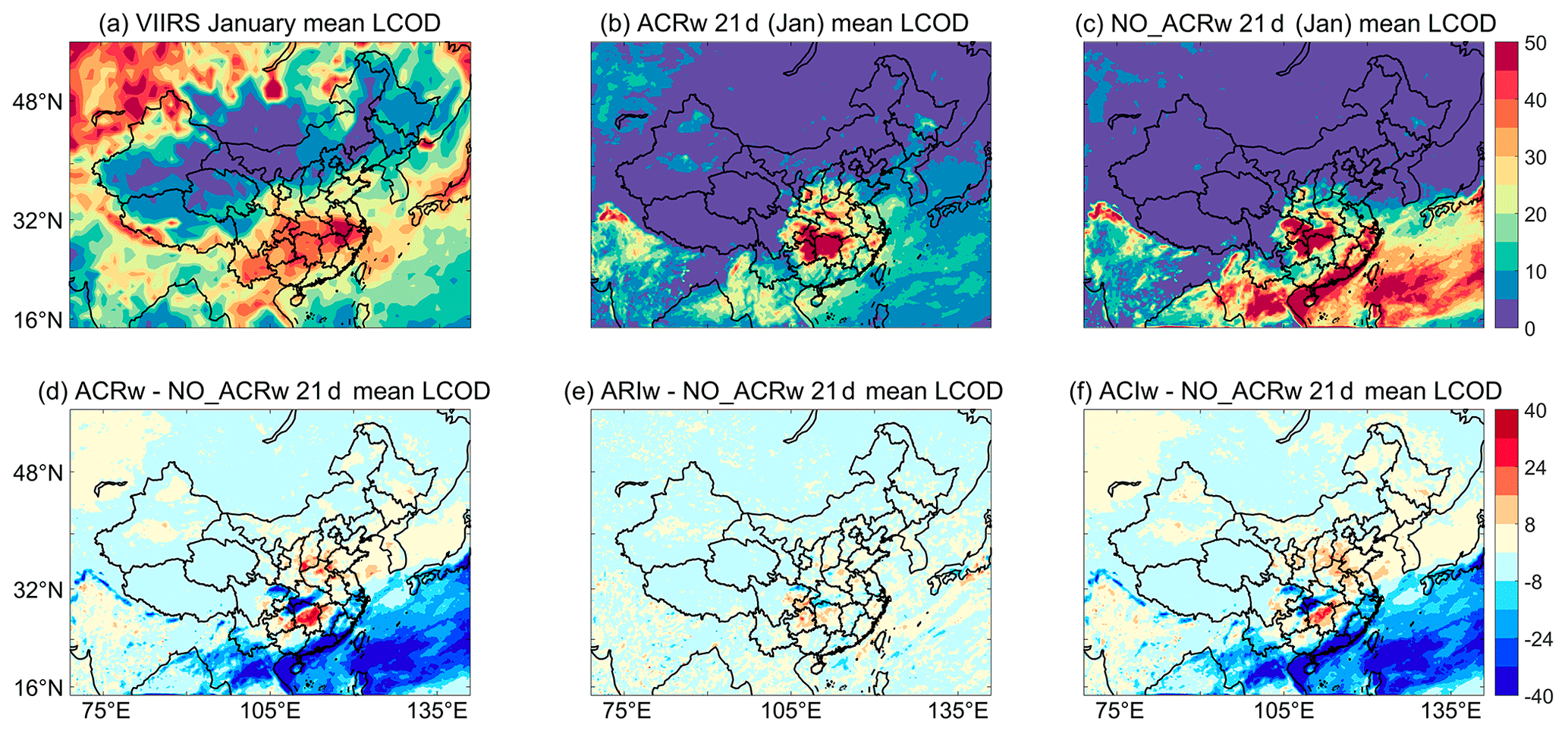
Figure 6 Mean LCOD from (a) VIIRS observations (monthly mean in during January 2015), (b) the Case ACRw simulation, and (c) the Case NO_ACRs simulation during 8 to 28 January 2015. Also shown are the differences in simulated LCOD between (d) Case ACRw and Case NO_ACRw, (e) Case ARIw and Case NO_ACRw, and (f) Case ACIw and Case NO_ACRw during 8 to 28 January 2015.

Figure 7 shows the monthly mean liquid cloud effective radii at cloud top from the Case ACRs simulation. Satellite retrievals of cloud effective radii often show large biases, except over areas dominated by liquid stratocumulus or stratus clouds (Yan et al., 2015; Witte et al., 2018). We instead compare the simulated liquid cloud effective radii to the reported values from aircraft observations over China. The observed effective radii of liquid cloud droplets over the NCP area in summer are in the range of 5.1 µm (±2.2 µm) to 6.3 µm (±2.3 µm) (Deng et al., 2009; Q. Zhang et al., 2011; Zhao et al., 2018). Over southern China, the observed effective radii of liquid cloud droplets in summer vary from 7.3 ± 1.7 to 7.9 ± 3.0 µm (Hao et al., 2017; Yang et al., 2020). Our simulated effective radii of liquid cloud droplets are consistent with these observed sizes of liquid cloud droplets and reflect the spatial difference between northern and southern China. The simulated mean effective radii are 8.4 ± 1.3 and 10.7 ± 0.9 µm over the NCP and southern China in July 2016, respectively.

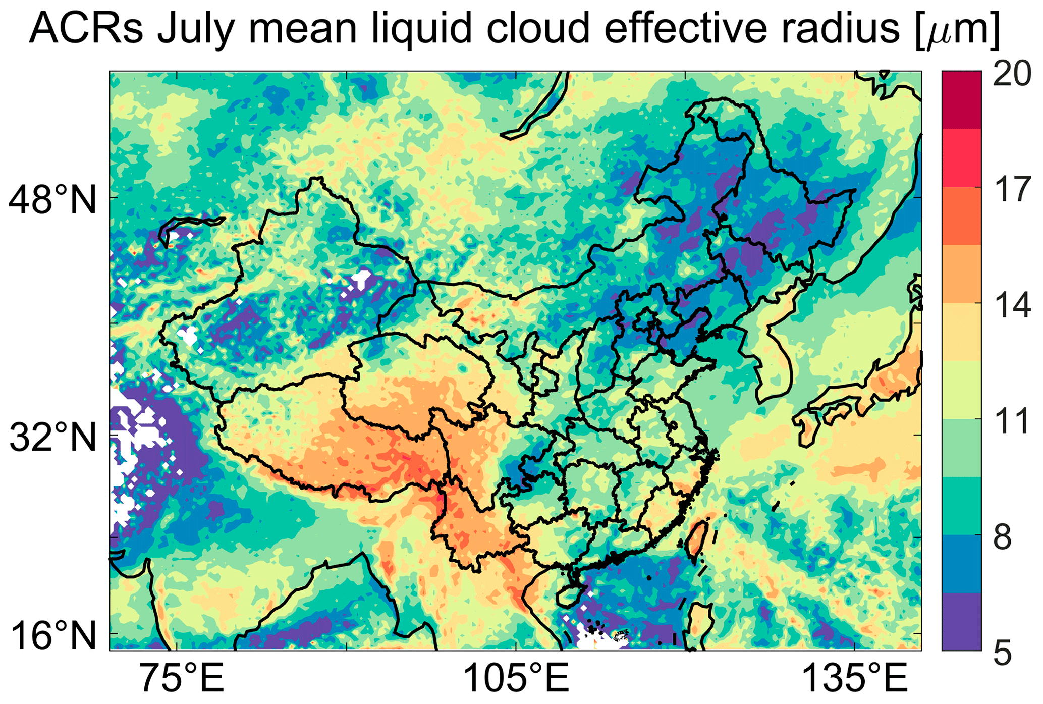
Figure 7 Monthly mean effective radii of liquid cloud droplets from the Case ACRs simulation during July 2016.

4.5 Validation of simulated regional surface meteorology

Figure 8a and b compare the surface downward shortwave radiation (SWDOWN) over East Asia from the EPIC-derived observations and those simulated by WRF-GC (Case ACRs) in July 2016. The simulated spatial distribution of July mean SWDOWN is in good agreement with the EPIC-derived observations over East Asia, with a spatial correlation coefficient of r = 0.73. The observed and simulated July mean SWDOWN over China are 288 ± 36 and 281 ± 48 W m⁻², respectively, with a slight low bias of −2.4 % in the model. Figure 9a and b compare the mean SWDOWN observed by CERES and that simulated by WRF-GC (Case ACRw) during 8 to 28 January 2015. The spatial distribution of the simulated wintertime SWDOWN also agrees well with the satellite observations, with a spatial correlation coefficient of 0.93 over the domain. The domain-average observed and simulated SWDOWN are 111 ± 45 and 140 ± 55 W m⁻², respectively (model NMB of 25.9 %). The overestimation of wintertime SWDOWN is over the Sichuan Basin, the Tibetan Plateau, and southern China, possibly related to the model's underestimation of AOD and LCOD over these areas in winter.

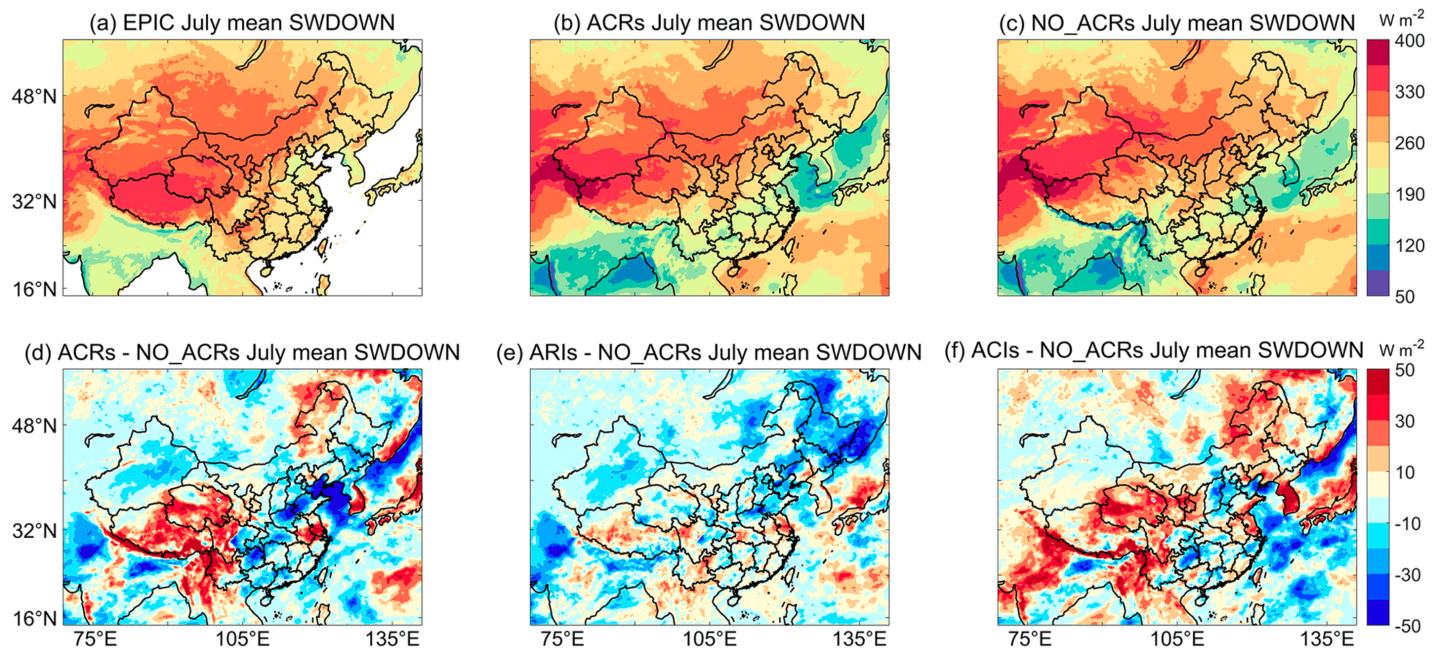
Figure 8 Monthly mean surface downward shortwave radiation (SWDOWN) from (a) EPIC-derived observations, (b) the Case ACRs simulation, and (c) the Case NO_ACRs simulation during July 2016. Also shown are the differences in simulated SWDOWN between (d) Case ACRs and Case NO_ACRs, (e) Case ARIs and Case NO_ACRs, and (f) Case ACIs and Case NO_ACRs during July 2016.

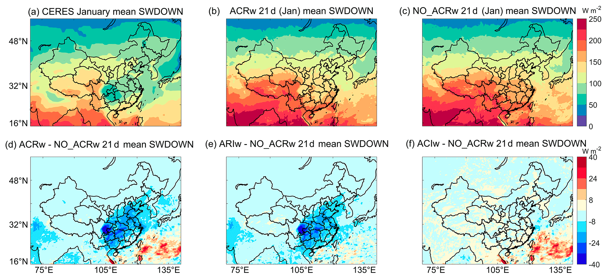
Figure 9 Mean surface downward shortwave radiation (SWDOWN) from (a) CERES observations (monthly mean in January), (b) the Case ACRw simulation, and (c) the Case NO_ACRw simulation during 8 to 28 January 2015. Also shown are the differences in simulated mean SWDOWN between (d) Case ACRw and Case NO_ACRw, (e) Case ARIw and Case NO_ACRw, and (f) Case ACIw and Case NO_ACRw during 8 to 28 January 2015.

Figure 10 Comparison of the observed (filled symbols) and simulated (filled contours) monthly mean surface air temperature from (a) Case ACRs and (b) Case NO_ACRs during July 2016. Also shown are the differences in simulated monthly mean surface air temperature between (c) Case ACRs and Case NO_ACRs, (d) Case ARIs and Case NO_ACRs, and (e) Case ACIs and Case NO_ACRs during July 2016.

Figure 11 Comparison of the observed (filled symbols) and simulated (filled contours) mean surface air temperature from (a) Case ACRw and (b) Case NO_ACRw during 8 to 28 January 2015. Also shown are the differences in simulated mean surface air temperature between (c) Case ACRw and Case NO_ACRw, (d) Case ARIw and Case NO_ACRw, and (e) Case ACIw and Case NO_ACRw during 8 to 28 January 2015.

Figures 10a and 11a show the good agreement between the simulated and observed surface air temperature over China during July 2016 (Case ACRs) and during 8 to 28 January 2015 (Case ACRw), respectively. The spatial correlation coefficients between the observed and simulated surface air temperature are 0.92 (Case ACRs) and 0.93 (Case ACRw), respectively. During July 2016, the simulated and observed surface air temperatures averaged over all sites are 23.7 ± 5.9 and 24.6 ± 5.0 ^∘C, respectively (NMB of −3.7 %). During 8 to 28 January 2015, the simulated surface air temperature averaged over all sites is 7.2 ± 6.7 ^∘C, with a model NMB of −13.3 % relative to the observations.

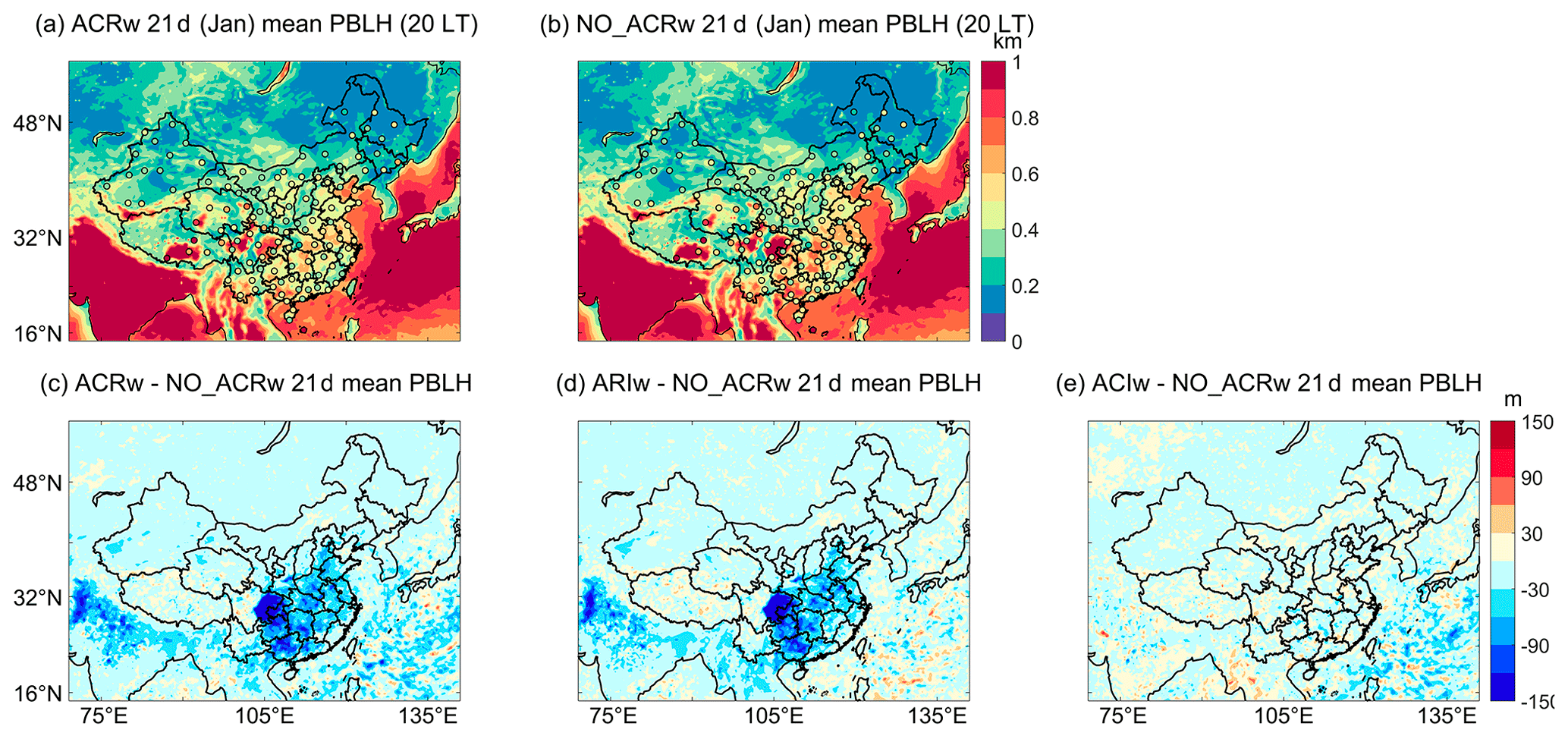
Figure 12 Comparison of the observed (filled symbols) and simulated (filled contours) mean PBLHs at 20:00 LT (12:00 UTC) from (a) Case ACRw and (b) Case NO_ACRw during 8 to 28 January 2015. Also shown are the differences in simulated PBLH at 20:00 LT (12:00 UTC) between (c) Case ACRw and Case NO_ACRw, (d) Case ARIw and Case NO_ACRw, and (e) Case ACIw and Case NO_ACRw during 8 to 28 January 2015.

Figure 12 compares the simulated (Case ACRw) mean PBLH at 20:00 LT to the rawinsonde observations over China during 8 to 28 January 2015. Lin et al. (2020) previously showed that, compared to the PBLH from the archived GEOS-FP reanalysis meteorology dataset, the wintertime PBLH simulated by WRF-GC better agreed with observations. This agreement is critical for the simulation of surface air quality, especially in winter (J. Wang et al., 2014; Z. Li et al., 2017). The WRF-GC simulated PBLH at 20:00 LT over China during 8 to 28 January 2015 is 462 ± 176 m, in good agreement with the observed 448 ± 129 m. At 08:00 LT (not shown), the model underestimates the observed PBLH by 34 % (simulated 281 ± 113 m versus observed 429 ± 94 m). Our validations above demonstrate the capability of the two-way coupled WRF-GC model (with ARI and ACI) in reproducing the regional meteorology.

4.6 Validation of simulated surface concentrations of PM_2.5 and ozone over China

We next assess WRF-GC's performance in simulating surface air pollutant concentrations over China in January 2015 and July 2016. We focus on wintertime PM_2.5 and summertime ozone, as they are the principle surface pollutants in China in winter and in summer, respectively. Figure 13a shows the observed and simulated (Case ACRw) PM_2.5 concentrations during 8 to 28 January 2015. WRF-GC reproduces the observed spatial distributions of PM_2.5 over eastern China (eastward of 108^∘ E); the spatial correlation between the observed and simulated PM_2.5 concentrations is 0.77. The simulated mean PM_2.5 concentration over eastern China (80.8 ± 32.6 µg m⁻³) is 9.3 % lower than the observations (89.1 ± 31 µg m⁻³). WRF-GC successfully captures the high PM_2.5 in central China and over the Sichuan Basin but underestimates the PM_2.5 concentrations over the NCP. WRF-GC also underestimates PM_2.5 over western China, likely reflecting a low bias in the model dust, also seen in the simulated AODs. WRF-GC reproduces the temporal variation of hourly PM_2.5 during 8 to 28 January 2015. The temporal correlation coefficient between the observed and simulated hourly PM_2.5 averaged over all Chinese sites is 0.77.

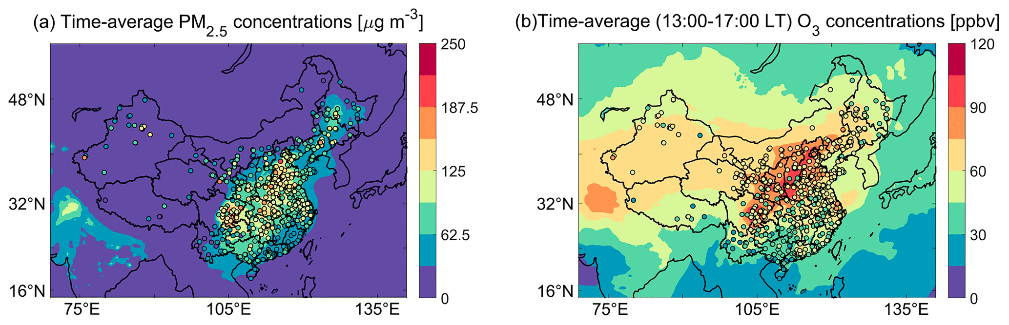
Figure 13 (a) Mean observed (symbols) and simulated (Case ACRw, filled contours) PM_2.5 concentrations during 8 to 28 January 2015; (b) mean observed (symbols) and simulated (Case ACRs, filled contours) afternoon surface ozone concentrations (13:00 to 17:00 LT) during July 2016.

Figure 13b compares the observed and simulated (Case ACRs) afternoon (13:00 to 17:00 local sun time; LST) surface ozone concentrations over China during July 2016. WRF-GC reproduces the higher surface ozone concentrations over northern and central China, the relatively lower ozone concentrations near the South China coast, and the ozone hotspots over the megacity clusters (the Beijing–Tianjin–Hebei area, the Yangtze River Delta area, and the Pearl River Delta area). However, the surface afternoon ozone concentrations simulated by WRF-GC (64 ± 17 ppbv) is biased high compared to the observations (51 ± 13 ppbv). The normalized mean bias of the simulation is 25.6 %. The overestimation of surface ozone concentrations is most severe over the Henan and Shanxi provinces in northern China. The temporal correlation coefficient between the observed and simulated hourly afternoon ozone concentrations averaged over all sites is 0.67. Our analysis demonstrates WRF-GC's general capability in reproducing the spatial patterns and temporal variations of Chinese surface PM_2.5 and ozone in winter and in summer, respectively, particularly over heavily polluted eastern China.

5 Impacts of ARI and ACI on simulated meteorology and air quality in China

5.1 Impacts of the ARI and ACI on chemistry-sensitive meteorology

We examine the individual and combined impacts of ARI and ACI on the simulated regional meteorological conditions. Table 5 summarized the comparison of the monthly mean meteorological variables simulated by the sensitivity experiments and the observations. Figures 5 and 6 show the impacts of ARI and ACI on the simulated LCOD in July 2016 and in January 2015, respectively. In both seasons, the simulated LCODs over eastern China agree best with the VIIRS observations when ARI and ACI are both turned on (Cases ACRs and ACRw) compared to the sensitivity simulations when ARI or ACI, or both, are turned off (Table 5). In particular, we find that the inclusion of ACI greatly reduces the simulated LCOD in both seasons; the inclusion of ACI corrects the high-biased LCODs simulated by Cases NO_ACRs and NO_ACRw, particularly over central and southern China, around Japan and Korea, and along the southern slopes of the Himalayas. In Cases ACRs and ACRw, the simulated monthly mean CCN concentrations (at 0.1 % supersaturation) averaged from the cloud bottom to cloud top are 150 and 58 cm⁻³, respectively. However, when ACI is turned off, WRF-GC uses a constant, high CCN activation rate (250 cm⁻³ per time step), leading to overestimation of cloud droplet numbers (effectively around 250 cm⁻³) and thus LCOD.

Table 5 Comparison of the simulated liquid cloud optical depth (LCOD), surface downward shortwave radiation (SWDOWN), and surface temperature (T2) from sensitivity experiments against satellite and surface observations during July 2016 and January 2015.

Figures 8 and 9 show the impacts of ARI and ACI on the simulated SWDOWN in July 2016 and January 2015, respectively. Again, the simulated SWDOWN values over China are most consistent with EPIC-derived and CERES observations, in terms of magnitudes and spatial correlations, when both ARI and ACI are turned on (Table 5). In July, the individual impacts of ARI and ACI on the simulated SWDOWN are comparable in magnitude but spatially different. Turning on ARI (Case ARIs) leads to 10 to 50 W m⁻² reductions in the simulated SWDOWN over northern and northeastern China, relative to the simulation where ARI and ACI are both turned off (Case NO_ACRs). Turning on ACI (Case ACIs) leads to 10 to 50 W m⁻² increases in the simulated SWDOWN over western and northeastern China and the Yangtze River Delta (YRD) area, as well as 10 to 30 W m⁻² decreases in the simulated SWDOWN over the NCP and southern China. In January, the inclusion of ARI reduces the simulated SWDOWN over eastern China by 8 to 40 W m⁻², while the inclusion of ACI does not significantly affect the simulated SWDOWN.

ARI and ACI also significantly affect the simulated surface air temperature. Figures 10 and 11 compare the simulated mean surface air temperature from the sensitivity experiments during July 2016 and January 2015, respectively. Again, the inclusion of both ARI and ACI leads to best agreement between the observed and simulated surface air temperature in both seasons (Table 5). In July, the inclusion of either ARI or ACI each leads to complex and spatially varied responses in surface air temperature (Fig. 10d and e). In January, the impacts of ARI on surface air temperature are much stronger than the impacts of ACI. Upon closer inspection, we find that the simulated responses of surface air temperature to ARI and ACI are spatially similar to the simulated responses of SWDOWN but with some exceptions. For example, over the Tibetan Plateau, the combination of ARI and ACI drives large increases in SWDOWN but does not lead to much higher surface air temperature. This may be because the inclusion of ACI reduced the simulated LCOD over the Tibetan Plateau, which may have increased the downward shortwave radiation while decreasing the downward longwave radiation, thus partially neutralizing the changes in the local net radiative balance.

The simulated PBLHs are also chemically sensitive, especially in winter. Figure 12 compare the simulated mean PBLH at 20:00 LT (12:00 UTC) from the sensitivity experiments during 8 to 28 January 2015. The simulated PBLH from Case ACRw (462 ± 176 m) better agrees with the observations (448 ± 129 m), compared to the simulated PBLH from Case NO_ACRw (491 ± 195 m). We find that the inclusion of ARI reduces the simulated PBLH throughout eastern China, particularly over the Sichuan Basin. This response is consistent with previous studies that showed the strong aerosol extinction in winter has a positive feedback to surface PM_2.5 concentration via the compression of PBLH (Z. Li et al., 2017; Zhang et al., 2018; Miao and Liu, 2019).

5.2 Impacts of ARI and ACI on simulated surface PM_2.5 over China in January 2015

Figure 14d, e, f show the combined and individual impacts of ARI and ACI on the simulated surface PM_2.5 concentrations during 8 to 28 January 2015, relative to the simulation when both ARI and ACI are turned off. Table 6 summarizes the assessment of the simulated surface PM_2.5 concentrations against surface measurements. The inclusion of ARI significantly increases the simulated surface PM_2.5 concentrations by 6 to 15 µg m⁻³ over parts of northern and southern China, and the Sichuan Basin, thereby improving the agreement with surface observations (Table 6; model versus observation slope of 0.97 in Case ACRw and 0.9 in Case NO_ACRw, respectively).

Figure 14 Differences in simulated monthly mean afternoon (13:00 to 17:00 LST) surface ozone concentrations during July 2016 (a) between Case ACRs and Case NO_ACRs, (b) between Case ARIs and Case NO_ACRs, and (c) between Case ACIs and Case NO_ACRs. Differences of simulated mean PM_2.5 concentrations during 8 to 28 January 2015 (d) between Case ACRw and Case NO_ACRw, (e) between Case ARIw and Case NO_ACRw , and (f) between Case ACIw and Case NO_ACRw. Stippled grids represent significant differences (two-tailed t test at 5 % significance level).

Table 6 Comparison between the PM_2.5 and afternoon ozone concentrations simulated by sensitivity experiments against the surface observations during July 2016 and January 2015.

Figure 12c, d, e show the combined and individual impacts of ARI and ACI on the simulated PBLH during 8 to 28 January 2015, relative to the simulation when both ARI and ACI are turned off. We find that the simulated response of surface PM_2.5 to ARI is spatially consistent with the simulated responses of SWDOWN, surface air temperature, and PBLH to ARI. Over the Sichuan Basin and parts of northern and central China, the strong aerosol extinction decreases the SWDOWN and surface air temperature, resulting in lower PBLH and a possibly more stable conditions within the PBL. The shallower and more stable PBL suppresses the dispersion of air pollutants, thus increasing surface PM_2.5 concentrations. These findings are consistent with previous studies (J. Wang et al., 2014; Z. Li et al., 2017; Zhang et al., 2018), although other feedback mechanisms may also play a role.

5.3 Impacts of ARI and ACI on simulated afternoon surface ozone over China in July 2016

Figure 14a, b, c show the combined and individual effects of the ARI and ACI on the simulated mean surface afternoon ozone concentrations in July 2016, relative to the Case NO_ACRs experiment. Overall, the inclusion of ARI and ACI in WRF-GC slightly reduces the model's positive bias in simulated surface ozone concentration (Table 6; model versus observation slope is 1.33 in Case ACRs and 1.38 in Case NO_ACRs, respectively). By including both ARI and ACI, the simulated July afternoon surface ozone concentration decreases by 2 to 10 ppbv over the Henan province, the Sichuan Basin, and parts of northeastern China. Over the YRD area and eastern Inner Mongolia, turning on ARI and ACI leads to increased afternoon surface ozone concentrations by up to 10 ppbv. These results are due to the spatially varied responses of surface ozone to ARI and ACI, respectively (Fig. 14).

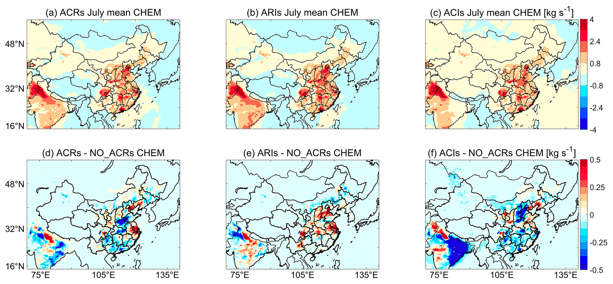
Figure 15 Mean simulated chemical mass tendency (unit: kg s⁻¹) for afternoon boundary-layer ozone from (a) Case ACRs, (b) Case ARIs, and (c) Case ACIs during July 2016. Also shown are the differences in simulated chemical mass tendencies for afternoon boundary-layer ozone between (d) Case ACRs and Case NO_ACRs, (e) Case ARIs and Case NO_ACRs, and (f) Case ACIs and Case the NO_ACRs in July 2016.

We further diagnose the net chemical mass tendency of the simulated ozone in the boundary layer over China during July 2016, to elucidate the mechanisms by which ARI and ACI affect boundary-layer ozone. The net chemical mass tendency (unit: kg s⁻¹) is the net rate of change of boundary-layer ozone mass due to chemical production and loss processes over each model grid, and its responses to ARI and ACI are shown in Fig. 15. We find that the spatial responses of the net chemical mass tendency of ozone to ARI and ACI are very similar to the simulated responses of surface afternoon ozone, SWDOWN, and surface air temperature to these chemical feedbacks (Figs. 8, 10, and 14). This indicates that ARI and ACI affect surface ozone mainly by modulating SWDOWN and surface air temperature, which in turn affect the emissions of biogenic isoprene and the subsequent chemical production of ozone in the boundary layer. For example, ARI leads to increased surface air temperature over the YRD area, while both ARI and ACI lead to increased SWDOWN over that area. These meteorological responses lead to enhanced local biogenic isoprene emissions and increased surface ozone. Over the Beijing–Tianjin–Hebei (BTH) area of China, where summertime ozone pollution is most severe (Lu et al., 2018), the effects of ARI and ACI are complex. ARI and ACI both reduce the local SWDOWN (Fig. 8e, f), while ARI increases surface air temperature over southern BTH and ACI suppresses surface air temperature over the entire BTH (Fig. 10d, e). The combined effect of chemical feedbacks is to increase surface ozone over the northern BTH, while decreasing surface ozone over southern BTH. ARI and ACI may also modulate other meteorological variables to affect surface ozone, and such possibilities warrant further investigation.

6 Conclusions

We present WRF-GC v2.0, an online two-way coupling of the WRF meteorological model and the GEOS-Chem chemical model, with aerosol feedback to radiation and cloud microphysics and nested-domain capability. The coupling structure of WRF-GC v2.0 is abstracted and modular, which allows the two parent models to be updated independently and stay state of the science. In addition, all WRF-GC v2.0 features can be parallelized using MPI, which allows the model to be computationally efficient and scalable to massively parallel architectures. WRF-GC v2.0 enables GEOS-Chem users to investigate the interactions between meteorology and atmospheric chemistry for any region at a wide range of spatial resolutions. At the same time, WRF-GC offers other regional modellers access to the GEOS-Chem chemical core.

We implement the ARI and ACI into WRF-GC v2.0 by adding three modules with the following functions: (1) diagnosing the size and number of the bulk aerosols simulated by GEOS-Chem, (2) computing aerosol optical properties, and (3) computing the number of aerosol particles activated into cloud droplets. The aerosol optical properties and cloud droplet number source are then passed to the WRF model for radiative transfer and cloud microphysics calculations. We develop WRF-GC's nested-domain capability by improving the state management module and the memory-management in GEOS-Chem (implemented as of GEOS-Chem version 12.4.0). The nested-domain capability enables WRF-GC simulations at higher spatial resolution.

Our test simulations show that the WRF-GC model with the aerosol–cloud–radiation interactions is able to reproduce the spatial distributions of wintertime surface PM_2.5 and summertime surface ozone with small biases compared with the observations. WRF-GC v2.0 also generally reproduces the spatial distributions of regional AOD and LCOD, SWDOWN, surface air temperature, and PBLH. Moreover, the inclusion of both ARI and ACI leads to the best agreement of simulated regional meteorology and surface air pollutant concentrations against observations, relative to sensitivity experiments where the chemical feedbacks are partially or completely excluded. We diagnose the response of wintertime surface PM_2.5 to ARI through modulation of surface air temperature and PBLH, as well as the response of summertime surface afternoon ozone to through modulation of radiation and temperature. ARI and ACI may also affect other meteorological variables to alter air quality; such possibilities may be further investigated using WRF-GC.

WRF-GC (v2.0) is the first coupling of GEOS-Chem to an open-source meteorological model with chemical feedbacks. The modules developed for WRF-GC v2.0 can also facilitate future two-way couplings between GEOS-Chem and other dynamical models. Support for the size-resolved aerosol schemes (APM and TOMAS) in WRF-GC is currently under development, which will better represent aerosol microphysics. We envision WRF-GC to become a powerful tool for research, forecast, and regulatory applications of regional atmospheric chemistry and air quality.