the Creative Commons Attribution 4.0 License.
the Creative Commons Attribution 4.0 License.
 | 22 Jun 2021
Retrieval of process rate parameters in the general dynamic equation for aerosols using Bayesian state estimation: BAYROSOL1.0
Aku Seppänen
Jari P. Kaipio
Kari E. J. Lehtinen
The uncertainty in the radiative forcing caused by aerosols and its effect on climate change calls for research to improve knowledge of the aerosol particle formation and growth processes. While experimental research has provided a large amount of high-quality data on aerosols over the last 2 decades, the inference of the process rates is still inadequate, mainly due to limitations in the analysis of data. This paper focuses on developing computational methods to infer aerosol process rates from size distribution measurements. In the proposed approach, the temporal evolution of aerosol size distributions is modeled with the general dynamic equation (GDE) equipped with stochastic terms that account for the uncertainties of the process rates. The time-dependent particle size distribution and the rates of the underlying formation and growth processes are reconstructed based on time series of particle analyzer data using Bayesian state estimation – which not only provides (point) estimates for the process rates but also enables quantification of their uncertainties. The feasibility of the proposed computational framework is demonstrated by a set of numerical simulation studies.
- Article
(6916 KB) - Full-text XML
- BibTeX
- EndNote


Aerosols scatter and absorb solar radiation and affect the permeability of the atmosphere to solar energy (the direct effect). In addition, aerosol particles act as seeds for cloud droplets (cloud condensation nuclei, CCN) and, thus, influence the properties of clouds (the indirect effect; e.g., Ramanathan et al., 2001). Worldwide, particulate air pollutants are also responsible for up to 7 million premature deaths per year (WHO 2014). The Intergovernmental Panel on Climate Change (IPCC Assessment Report 2013 by Stocker et al., 2014, and IPCC Assessment Report 2014 by Pachauri et al., 2014) recognized the uncertainty in the radiative forcing caused by aerosols as the main individual factor limiting the scientific understanding of future and past climate changes.
Some of the uncertainty is caused by the fact that the initial stages of the new particle formation (NPF) processes in the atmosphere are still not completely known. It has been known for close to 100 years that photochemically driven NPF may occur in the atmosphere (Aitken, 1889). The fact that it occurs regularly throughout the troposphere has, however, only become clear during the last 15 years or so (Kulmala et al., 2004). Partly because of this, the systematic development of parameterizations describing tropospheric NPF as an active research topic has only just begun. Studies with these models suggest that tropospheric NPF may have significant effects on CCN and, in turn, on the general global cloud albedo effects of atmospheric aerosols (Merikanto et al., 2010). One challenge in estimating the anthropogenic aerosol effect on climate is the need to know the preindustrial conditions and dynamics, which is the baseline of forcing estimations (Hansen et al., 1981). Very recently, Gordon et al. (2016) made new estimations of anthropogenic aerosol radiative forcing by assuming pure biogenic particle formation, as suggested by Kirkby et al. (2016) based on the Cosmics Leaving Outdoor Droplets (CLOUD) experiment at CERN. The increased particle formation rates under preindustrial conditions increased the CCN conditions as well as the cloud albedo – resulting in a 0.22 W m−2 decrease in anthropogenic aerosol forcing. As the NPF treatment in global climate models is typically based on parameterizing particle formation and growth rates (GRs) from chamber experiments such as CLOUD or from field measurements, it is of great importance to analyze the data with care and pay attention to uncertainties.
Most of the research dealing with NPF event analysis has used similar methodology as outlined in the “protocol” described by Kulmala et al. (2012) and Dada et al. (2020). Particle formation rates, at the detection limit of the instrument (typically in the range from 2 to 3 nm), are usually estimated from the time evolution of either the total number concentration or the number concentration below a certain size (e.g., 20 nm), correcting for coagulation loss and condensation growth with very simple and approximate balance equations. For condensational growth rate, there have been three main approaches: (1) fitting the growing nucleation mode with a lognormal function, and the growth of the mode GR is defined as the growth of the geometric mean size of the mode (Leppä et al., 2011); (2) the so-called “maximum concentration method” in which GR is estimated from the times when each measurement channel of the instrument reaches its maximum concentration (Lehtinen and Kulmala, 2003); and (3) the so-called “appearance time method” in which GR is estimated from concentration rise times of each channel (Lehtipalo et al., 2014). Methods 1 and 2 are applicable to cases in which there is a clear nucleation mode growing, as is the case, for example, for the multitude of events analyzed from the Hyytiälä forest station in Finland (Maso et al., 2005). For chamber experiments, where the aerosol size distribution approaches steady state (Dada et al., 2020), these two approaches cannot be used. Method 3 can then be applied to the transition stage of the dynamics, before steady-state is reached. All of these methods suffer from disturbances by other aerosol microphysical processes (e.g., coagulation and deposition) and, in addition, cannot be used to estimate uncertainties related to GR. Deposition rates are typically estimated by targeted experiments with either several different experiments with different monodisperse aerosol or in the absence of vapors and with low enough concentrations that other microphysical processes do not affect the estimation.
The last decade has been a huge leap forward in atmospheric NPF research. Instrument development, especially advances in particle detection efficiency and mass spectrometry, have allowed us to measure details of the dynamics of the smallest clusters (e.g., Almeida et al., 2013). At the same time, however, potentially superior advanced data analysis methods have not been used. Instead, NPF and particle growth rates have been analyzed with the abovementioned very simple regression or balance equation approaches (an overview of the typical methods is given in Kulmala et al., 2012), suffering from potentially crude approximations and permitting no proper estimation of the uncertainties. It is likely that there are significant inaccuracies in quantities such as particle formation and growth rates estimated previously, and at least their uncertainties have typically not been quantified. Very recent studies by Kürten et al. (2018) have already shown that the difference between nucleation rates estimated by fitting a sophisticated aerosol model to data and a “traditional” simple method can be as large as a factor of 10.
Studies on applying computational inversion methods to estimating the most important quantities of interest with respect to particle fate and effects in the atmosphere, the formation and growth rates, are rare. Lehtinen et al. (2004) applied simple least-squares-based optimization of aerosol microphysics to measured data. This method was later improved (more processes, less assumptions) by Verheggen and Mozurkewich (2006) and Kuang et al. (2012). These studies, however, did not address the uncertainties in the estimated parameters. Henze et al. (2004) used the method of adjoint equations to estimate condensation rates based on measured evolution of the aerosol size distribution. Sandu et al. (2005) presented adjoint equations of the complete aerosol general dynamic equation (GDE) which could be a basis for data-assimilation of aerosol dynamics. We are, however, not aware of the methodology being used later.
In the statistical (Bayesian) framework of inverse problems (Kaipio and Somersalo, 2006), the uncertainties of the model quantities are modeled statistically, and it offers an approach to uncertainty quantification, in addition to parameter estimation. In a time-invariant case, the Bayesian approach was adopted to estimate aerosol size distributions by Voutilainen et al. (2001). Thus far, the only works where the statistical approach has been taken to inverse problems in aerosol size distribution dynamics are those on parameter estimation in aggregation–fragmentation models (Ramachandran and Barton, 2010; Bortz et al., 2015; Shcherbacheva et al., 2020), estimating the size distribution evolution using Kalman filtering (Voutilainen and Kaipio, 2002; Viskari et al., 2012) and estimating evaporation rates using a Markov chain Monte Carlo method (Kupiainen-Määttä, 2016). However, the statistical inversion framework (and Bayesian state estimation in particular) has been applied to several other problems which are mathematically similar to parameter estimation in aerosol dynamics. Unknown coefficients have been estimated in, for example, Fokker–Planck equations (Banks et al., 1993; Dimitriu, 2002), age-structured population dynamics models (Rundell, 1993; Cho and Kwon, 1997) as well as algal and phytoplankton aggregation models (Ackleh, 1997; Ackleh and Miller, 2018).
In this paper, we approach the problem of estimating unknown rate parameters in the aerosol general dynamic equation in the framework of Bayesian state estimation. We model the discretized particle size distribution as well as the unknown nucleation, growth and deposition rates in GDE as multivariate random processes, and estimate them from sequential particle counter measurements using the extended Kalman filter (EKF) and fixed interval Kalman smoother (FIKS). The feasibility of these estimators to quantify the process rate parameters and their uncertainties is tested with series of numerical simulation studies.
The temporal evolution of the aerosol size distribution can be described by a population balance equation referred to as the GDE (Zhang et al., 1999; Prakash et al., 2003; Lehtinen and Zachariah, 2001; Smoluchowski, 1916; Friedlander and Wang, 1966). We write the continuous form of the GDE as
where dp is the particle diameter and t is time. Further, denotes the condensational growth rate, is the coagulation frequency and is the deposition rate.
The boundary conditions consist of fluxes of particles in and out of the considered size range . In reality, the formation of particles occurs at very low size (typically at the 1.5–2 nm scale) by nucleation; the theoretical size at which molecule clusters start being stable is referred to as the critical size, and it is denoted in Eq. (1). Note that we do not include an explicit source term in Eq. (1) to model the true nucleation (spawning particles out of vapor) as we are considering typical size ranges for particle mobility measurements (differential mobility particle sizer, DMPS, or scanning mobility particle sizer, SMPS) which are above the nucleation size. In practice, this means that is always chosen to be sufficiently larger than the critical size . The appearance of new particles to the measurement range then occurs by condensational growth of freshly nucleated particles from below the measurement range. This process, sometimes called apparent particle formation (e.g., Lehtinen et al., 2007), is conveniently treated as a particle-concentration flux, in particle-size space (), as a boundary condition for the GDE. Hence, the nucleation J=J(t) is identified with the flux of particles to the smallest size class by condensation – that is,
Similarly, for the outward flux of particles at the largest size class, we write
which states that the growth of particles to a size exceeding , the upper limit of the size range, is negligible.
The time- and/or size-dependent parameters g, β, λ and J characterize the microphysical properties of aerosols: these parameters, along with boundary conditions of the GDE, completely determine the evolution of the aerosol size distribution. However, the process rate parameters are usually not known. In this paper, we aim at estimating the growth, deposition and nucleation rates (g, λ and J, respectively) based on particle size distribution measurements. For the coagulation coefficient β, a fixed (known/approximate) value will be used.
The analysis proposed in this paper is applicable to both differential mobility particle sizer (DMPS) and scanning mobility particle sizer (SMPS) measurements. For the rest of the paper, however, we refer to measurement modality as SMPS because the number of particle size classes is relatively high in the numerical example cases.
An SMPS measurement is vector yk∈ℝM that represents an indirect observation of the particle size density n(dp,tk), corrupted by Poisson distributed noise:
where V is a constant (the effective volume of the sample in the condensation particle counter), ℋ is a device-dependent linear operator and M is the number of channels in the particle counter. In the following, we assume that the rate of time evolution is negligible compared with the time required to measure M channels, or one frame, with an SMPS. We denote the measurement time of the kth frame by tk.
As SMPS measurements explicitly depend on the size density n alone and not on g, λ and J, a measurement yk corresponding to a single time instant does not carry enough information to estimate these parameters. However, as g, λ and J determine the temporal evolution of n, it might be possible to estimate them on the basis of a sequence of measurements yk corresponding to a set of time instants tk, .
In this section, we formulate the problem of estimating the time-dependent size density n and the process rate parameters g, λ and J as a Bayesian state estimation problem. To this end, we first discretize the GDE with respect to size and time, and write it in a stochastic form in order to model its uncertainties. We also model the process rate parameters as discrete-time stochastic processes. This formulation allows us to express the following questions in the Bayesian framework (Gelb, 1974):
-
What are the expected values of n(dp,tk), g(dp,tk), λ(dp,tk) and J(tk) at each time tk given a set of measurements corresponding to discrete times ?
-
How large are the uncertainties of the estimated quantities?
The state estimation problems are referred to as prediction, filtering and smoothing depending on whether ℓ<k, ℓ=k or ℓ>k, respectively. While filtering is a suitable choice for online monitoring and control problems, smoothing is usually a preferable choice when estimates are not needed online; the smoother estimates also utilize the future observations for the estimate corresponding to time tk.
The latter question refers to posterior uncertainties – that is, uncertainties of the quantities given the measurements Yℓ. In the Bayesian framework, these uncertainties can be quantified by computing, for example, posterior variances and credible intervals of the parameters.
In the simplest special case, where the evolution model and observation model are linear with respect to all parameters and all error terms are additive and Gaussian, the Bayesian filtering and smoothing problems can be solved by Kalman filter and Kalman smoother recursions, respectively (Kalman, 1960; Gelb, 1974). In general cases, where models are nonlinear or non-Gaussian, only approximate solutions are available. In principle, the best approximations of the posterior estimates are obtained with sequential Monte Carlo methods, known as particle filters/smoothers (Särkkä, 2013). However, these methods are limited to small dimensional cases, because of the high computational burden. Computationally more efficient approximations include ensemble, unscented and extended Kalman filters/smoothers (Särkkä, 2013). In this paper, we choose the extended Kalman filter (EKF) and fixed interval Kalman smoother (FIKS), but we note that the other filters and smoothers developed for nonlinear state estimation are applicable as well. In the next section, the feasibility of the EKF and FIKS for the GDE parameter estimation problem will be tested numerically.
2.1 Evolution model
2.1.1 Discretized, stochastic GDE
To approximate the GDE (1) numerically, we partition the particle size variable dp into Q intervals (or bins) Ωi of widths Δdi, . The discrete instants in time in the temporal discretization are denoted by tk, , and the differences between consecutive times are denoted by . We denote the number concentration of particles corresponding to the ith bin at time tk by – that is, , and a vector consisting of particle concentrations in all Q bins at time tk by Nk, that is, . We discretize the condensation and deposition rates accordingly, and write , . Further, the nucleation J is discretized with respect to time: Jk denotes the nucleation rate at time tk.
Using Euler's method for time integration and first-order upwind differencing for the condensation terms, we get the discrete-time evolution model for the particle number concentrations in bins Ωi (Korhonen et al., 2004):
where Ci(Nk) is a nonlinear coagulation term; for details, see Lehtinen and Zachariah (2001). Here, the choice for approximating the derivative in the growth term in the discretization of the GDE is made, assuming that the particle growth rate is positive. The modification to cases where the aerosols evaporate, i.e., where growth rate is negative, is straightforward. Such a time discretization scheme can become unstable; however, it is possible to apply a different method, e.g., implicit Euler or Crank–Nicholson (Trangenstein, 2013). Equations (5) and (6) can be written equivalently in vector form as
Here, is a sparse matrix consisting of elements Aij:
is a vector of the form , and the nonlinear term C(β,Nk) is defined accordingly.
Finally, we complement the discretized GDE with a stochastic term ϵk∈ℝQ to account for modeling errors caused by factors such as discretization and uncertainties of the boundary conditions, and we write
where is of the form . In this paper, the stochastic state noise term ϵk is modeled as Gaussian, , where Γϵ is the covariance matrix of ϵk. Equation (9) forms a discretized, stochastic evolution model for the particle number concentration N.
2.1.2 Models for the parameters of the GDE
All the unknown parameters of the GDE (g, λ and J) are known to be nonnegative. For this reason, we reparametrize these quantities by writing , and , where ξg,i, ξλ,i and ξJ are the (unconstrained) parameters, and mappings Pg, Pλ, PJ have the form of a so-called softplus function (Dugas et al., 2001) :
Note that this parameterization only constrains the parameter from below, but if an upper boundary is known, the function in Eq. (10) could be changed in favor of, for example, a logistic function which allows for both constraints from below and from above. We denote the vectors consisting of all condensation and deposition parameters at time tk by and , respectively.
As the process rates g, λ and J in the GDE are time-varying, the state estimation requires one to model their time dependence. In this paper, we model ξg,i, ξλ,i and ξJ as either first-order Markov processes,
where Ψφ is a diagonal matrix Ψφ=rφI, and , or as second-order Markov processes,
with and . In both models, stands for Gaussian noise . To simplify the following description, we assume all the models to be of the form shown in Eq. (11), but we note that the extension to second-order models is straightforward: higher-order Markov models can be converted into the form of first-order Markov models by augmenting the state variables corresponding to more than one time instant into a single vector. The second-order models are suitable for some of the quantities in GDE, because they imply temporal smoothness of those processes (Kaipio and Somersalo, 2006). The specific choices of the state models and their parameters are discussed in Sect. 3 and specified in Appendix B.
The evolution models, such as Eqs. (11) and (12) can be argued to be unrealistic, as they are not based on physics. The understanding, however, is that if the (co)variances of the driving noise processes are set high enough, such models are feasible in the sense that the actual are well supported by the modeled distribution of . Systematic (state-space identification) approaches exist that allow one to test the model's feasibility against the driving noise distribution (variances) (Gelb, 1974). In the next section, we test the state estimation based on the above models in cases where the true evolution of the quantities is not of the form of Markov models.
2.1.3 Augmented evolution model for n, g, λ and J
To complete the evolution model, we define an augmented state variable Xk,
and combine the evolution models written in Sects. 2.1.1 and 2.1.2, yielding
or
This is the evolution model for the augmented state variable Xk, which includes not only the number concentrations of the size sections but also the unknown process rates. Next, we write the observation model in terms of Xk, and then, in Sect. 2.3, we apply Bayesian state estimation to infer Xk, based on sequential SMPS measurements.
2.2 Observation model
An SMPS consists of a differential mobility analyzer (DMA), which classifies charged particles based on their mobility in an electric field, and a condensation particle counter (CPC) where the classified particles are grown to sizes detectable, for example, optically. All particle counters provide only discrete, indirect and noisy data on the particle size distributions. Mathematically, each channel in a particle counter gives data that corresponds to a convolution/projection of the particle size distribution onto a space spanned by device-specific kernel functions; moreover, the counter data are corrupted by Poisson distributed noise.
2.2.1 SMPS transfer function
The output of each DMA is the detected number concentration in a size class; in channel i corresponding to a discrete time index k, it is of the form
where Ψi(dp) is a time-invariant kernel function; ωi is the support of Ψi(dp) – that is, the set of points where Ψi(dp) is nonzero; t0 is the initial time; and Δt is the duration of counting particles in the CPC for a single channel. Further, V is the volume of the aerosol sample that passes through the CPC counter with a detector–sample flow rate ϕa(t) in the period of time Δt – that is, .
2.2.2 CPC counting model
The measurement data of the ith channel of an SMPS, , consist of Poisson-distributed counts given by the CPC:
where is the volume of sample used in the CPC for counting. In the numerical studies of this paper, we use this model when simulating the measurement data. In state estimation, however, we approximate the Poisson distributed observations as Gaussian:
where γi is the approximate variance of the noise. In this paper, we use the same approximation as in Voutilainen et al. (2000) and write .
By discretizing the SMPS model (Eq. 16) and using the above Gaussian approximation of the noise, we write an observation model of the form
where , is an observation matrix and is the Gaussian observation noise . Here, the covariance of the observation noise is of the diagonal form . The additional noise term, ιk is included in Eq. (19) in order to account for errors caused by the discretization of the measurement operator in Eq. (16). Here, ιk is simply approximated as being Gaussian distributed with zero-mean whose components are calculated as mutually independent; hence, the covariance matrix is of diagonal form. Furthermore, the approximation error term ιk is assumed to be independent of the counting noise ; thus, the total error , where . For a more rigorous approach to handling modeling errors, we refer to the book by Kaipio and Somersalo (2006).
Finally, the model (Eq. 19) can be written in terms of the state variable Xk defined in Eq. (13),
where H is a block matrix of the form .
2.3 State estimation
The nonlinear evolution model (Eq. 15) and the linear observation model (Eq. 20) form a system
referred to as the state-space representation. The system is stochastic due to the state noise and observation noise processes, wk and ek, respectively. In addition, we model the initial state X0 as a Gaussian random variable . Given this model, we can state the Bayesian filtering and smoothing problems as follows: form the conditional probability density of the random variable Xk, given the sequence of measurements . In the extended Kalman filter and smoother, these probability densities π(Xk|Yℓ), are approximated by Gaussian densities – that is,
where Xk|ℓ and Γk|ℓ are approximations of the respective conditional expectation and covariance of Xk given Yℓ (Gelb, 1974).
Kalman filtering gives online estimates π(Xk|Yk) based on
the data set from the beginning up to the present time k – that is, ℓ=k,
whereas in smoothing ℓ>k. In the FIKS, in
particular, ℓ=K, where K is the index of the final time step. In
other words, the FIKS estimate π(Xk|YK) at each time k is
based on the entire data set from the beginning to the end of measurements.
The EKF and FIKS estimates (approximate expectations Xk|ℓ and
covariances Γk|ℓ) are given by the following forward and backward
iterations (Gelb, 1974):
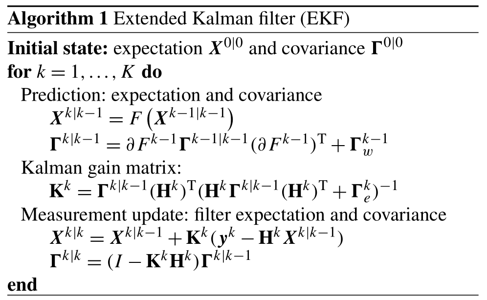
In Algorithms 1 and 2, ∂Fk denotes the Jacobian matrix of the nonlinear mapping F at point Xk|k. Note that the FIKS is based on a backward recursion, which starts from the filter estimate corresponding to final state: XK|K, ΓK|K.
In this section, the feasibility of the proposed estimation scheme is tested with numerical studies, where the aerosol particle evolution is simulated by numerical approximations of the GDE corresponding to a set of process rates, and where synthetic SMPS data are computed by numerical modeling of the DMA and generating the Poisson-distributed CPC data. Two type of events are considered: in cases 1 and 2, the evolution of the aerosol size distribution is governed by a nucleation event (NE) and the subsequent growth of the nucleation mode in a background of existing aerosols; in cases 3 and 4, new particles are formed in a continuous nucleation process and their further evolution is controlled by condensational growth and deposition, so that the size distribution approaches a steady state (SS). In all cases, the particle growth is dominated by condensation, and the loss of particles (caused by wall deposition, sedimentation, dilution, etc.) depends linearly on the size distribution function. Further, the coagulation kernel is chosen to have the form given in the book by Seinfeld and Pandis (2016). In these numerical studies, cases 1 and 2 (NE) qualitatively represent a typical particle formation event in the atmosphere (e.g., Hyytiälä Maso et al., 2005), whereas cases 3 and 4 (SS) represent particle formation and growth in a chamber experiment (e.g., CLOUD Lehtipalo et al., 2014).
3.1 Cases 1 and 2: nucleation event (NE)
3.1.1 NE: data simulation
In the numerical simulation study, the temporally evolving particle size distribution is synthetically generated using the (deterministic) discretized GDE model described by Eqs. (5) and (6) with predefined process rates g,λ, β and J. In the estimation, however, g,λ and J are, of course, not known.
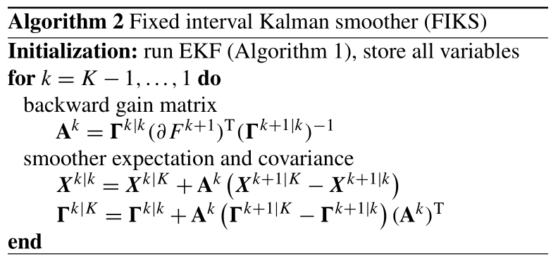
In the NE case, the process rates g,λ and J are chosen to have the following properties: the condensational growth rate g is independent of the particle size but depends on time, whereas the loss rate λ depends on particle size but not on time. Further, the nucleation rate J is a time-dependent, continuous function which represents an NE in a time interval and is zero in all other instants within the period of interest [0,15 h]. As noted above, the coagulation kernel is known, yet the coarse discretization also causes error in this term. The detailed forms of the process rates are shown in Table A1 (Appendix A).
When simulating the evolution of the particle distribution, the particle diameter is discretized into Q=2500 logarithmically distributed bins. Such a high size resolution is chosen in order to avoid numerical diffusion effects and to obtain a good approximation of the particle size density. The time step Δtk in the explicit Euler time integration scheme is chosen based on the Courant–Friedrichs–Lewy condition (Courant et al., 1928; Dullemond and Dominik, 2005):
The CFL criterion is applied in order to keep the time integration stable with respect to condensational growth and loss. The coagulation rates are not considered here because coagulation is actually a dampening mechanism that stabilizes time integration. The nucleation, growth and loss rates as well as the resulting particle size density evolution for the NE cases are illustrated in Fig. 1.
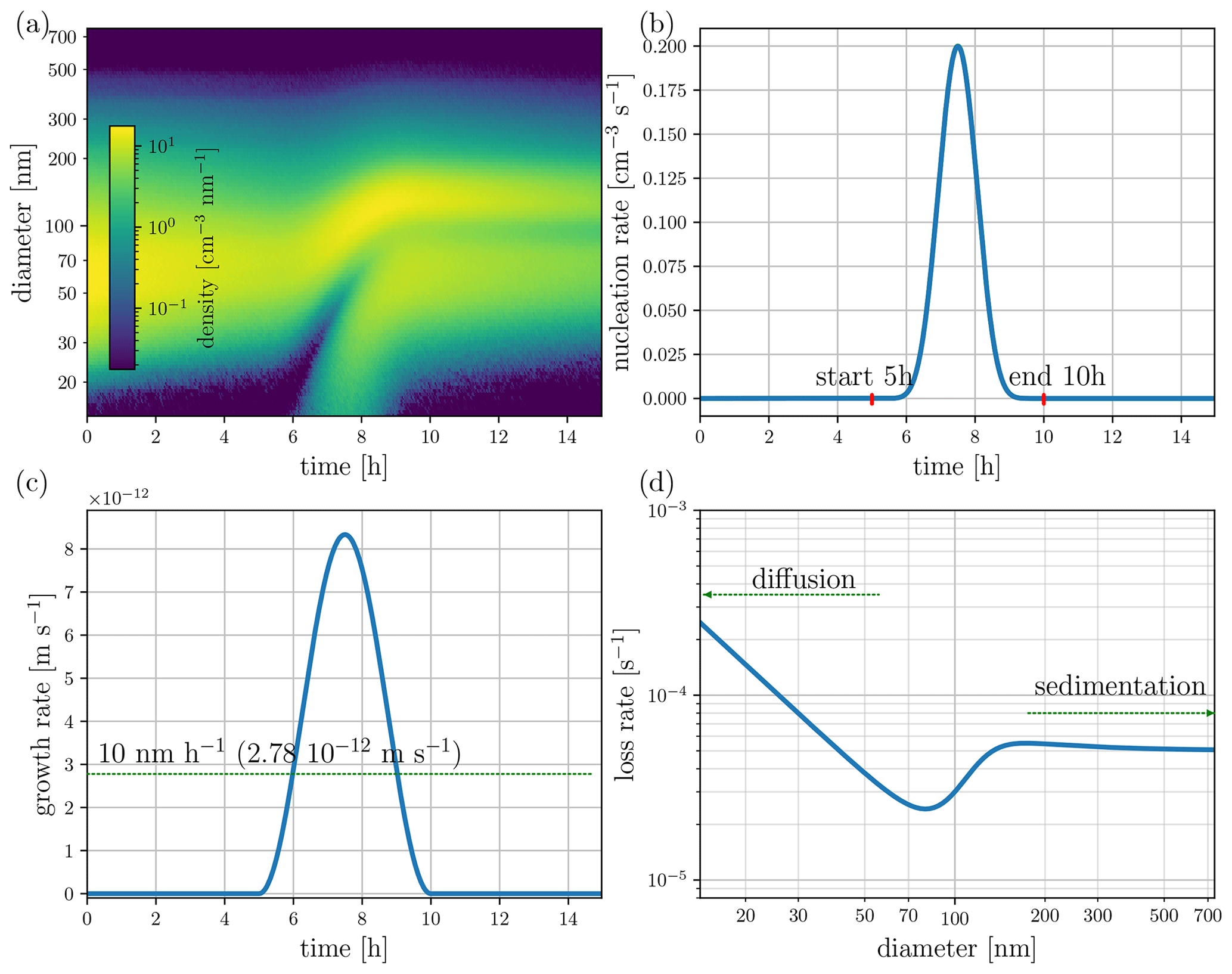
Figure 1Cases 1 and 2 – a nucleation event, showing true (simulated) processes: (a) particle size density (measurement), (b) nucleation rate, (c) growth rate and (d) loss rate.
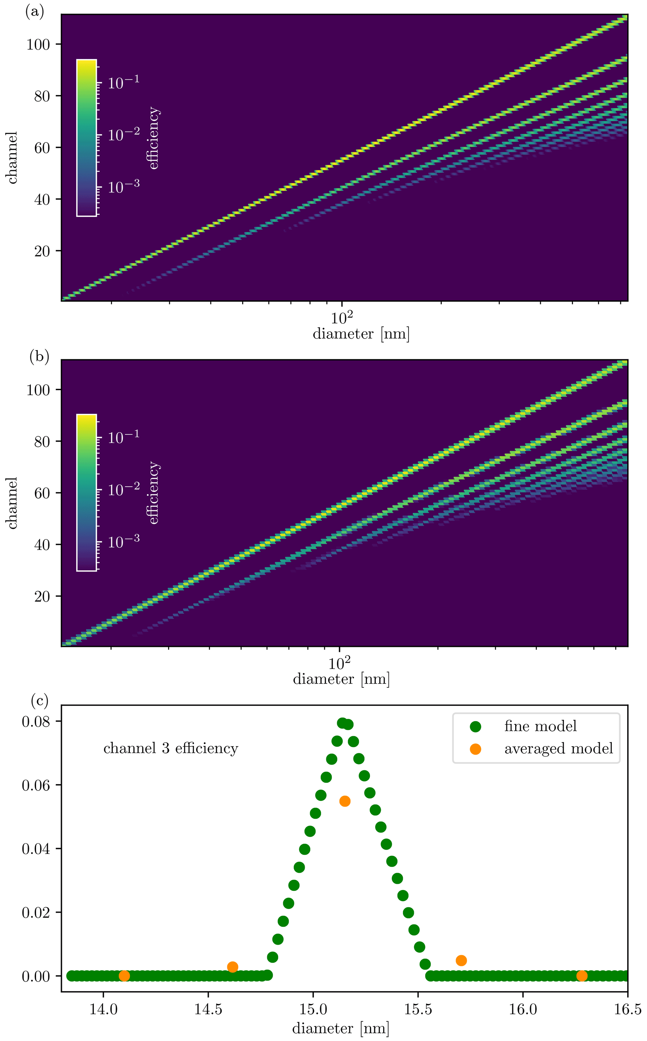
Figure 2The size distribution transfer functions for (a) simulating the measurement data, and (b) the observation model used in state estimation. In the images, the horizontal axis corresponds to the size of the particle entering the device, and the vertical axis represents the channels of the SMPS. The colors represent the values of the efficiency with which a given particle size will be classified in a given bin in the particle sizer.
As explained in Sect. 2.2, the measurements consist of simulated counts modeling CPC combined with DMA. The model for the kernel functions Ψi(dp) corresponds to an SMPS 3936 device, and it accounts for the most relevant effects (Millikan, 1923; Stolzenburg, 1989; Flagan, 1998; McMurry, 2000; Boisdron and Brock, 1970; Wiedensohler, 1988). We skip the details here, and only visualize the kernels, by plotting the size-distribution transfer function, or the observation matrix , as a color map (Fig. 2a).
We simulate the synthetic CPC measurement corresponding to each CPC channel i at each time k by drawing samples from a Poisson distribution, given in Eq. (17) with mean . As the expectation of is and its variance is , the signal-to-noise ratio (SNR) of CPC data increases with V. In order to investigate the effect of SNR to the process rate estimates, we generate the Poisson-distributed observations corresponding to two sample volumes: V=90 cm3 (Case 1: NE, high SNR) and V=0.9 cm3 (Case 2: NE, low SNR). In Case 1, the range of SNR was [0,6426]; in Case 2 it was [0,64.26].
3.1.2 NE: parameter estimation
In this section, we briefly describe the assumptions made when constructing the models used for computing the state estimates in the NE cases. The exact forms of the models as well as choices of parameters are listed in Appendix B.
For the evolution models used in state estimation, the particle size range [14.1 nm, 736.5 nm] is divided into 111 bins – that is, the size range is narrower and the discretization is significantly coarser than when simulating the data. The GDE-based, discrete stochastic state evolution model (Eq. 9) for the particle number N is written as described in Sect. 2.1.1. The covariance matrix Γϵ of the stochastic term ϵk is chosen to be of diagonal form.
In this case study, we assume to know that the condensation rate is time dependent but size independent. Moreover, both the condensation and nucleation rates are assumed to be temporally smooth, and we model them as second-order stochastic processes (Eq. 12). The loss factor λ is assumed to be a smooth function of the particle size. Further, we write a first-order Markov model (Eq. 11) for its temporal variation – that is, although the true loss factor is time invariant, we do not assume to know this property in state estimation. This is done to study the stability of the estimation scheme: although the deposition loss is modeled as varying with time, the estimation should yield essentially time-invariant estimates.
The covariance of the initial state, Γ0|0, is chosen to be diagonal; this signifies that the elements of X0 are mutually independent. Moreover, the variances of X0 are chosen to be relatively large in comparison with the variances of the state noise vector ϵk; this indicates a high uncertainty of the initial state. We note that the selection of the parameters in the stochastic terms is a crucial part of the state-space model. However, the state estimates are not extremely sensitive to these choices; choosing parameters that are of the right order of magnitude is usually enough, and as the stochastic models are written for physically relevant quantities, ballpark ranges of the parameters are often available a priori.
The size-distribution transfer function corresponding to the discretization of the particle size in estimation is illustrated in Fig. 2b. The approximate observation model is used in order to avoid so-called inverse crime, which refers to the use of unrealistically accurate models in the inversion of simulated data. A comparison between the true transfer function and the approximated one used in the estimation – mean over each discretization bins – is depicted in Fig. 2c for the third channel. Furthermore, as noted in Sect. 2.2, instead of using the Poisson model for the measurements, the observation noise is approximated as additive and Gaussian. This choice is made for computational convenience, as it allows for the direct applications of EKF and FIKS into the state-space system.
The extended Kalman filter and smoother estimates are computed using Algorithms 1 and 2, respectively. From the resulting state estimates Xk|ℓ, the approximate posterior expectations of the processes are computed using the models , and (see Sects. 2.1.2 and 2.1.3). We also compute approximate 68 % credible intervals of the estimates, by mapping the values , to the corresponding process rate spaces. Note, however, that due to the linearizations/Gaussian approximation behind EKF, these approximate intervals do not necessarily represent the ranges where the true parameter value lies; these are the ranges within which the true value most likely lies with an 0.68 probability. In the following, we refer to these approximate credible intervals as“posterior error intervals”.
3.1.3 NE: results and discussion
The results of Case 1 (NE, high SNR) are illustrated in Fig. 3. The figure shows the Kalman smoother estimates for the particle size density, and the EKF and FIKS estimates for the growth, apparent particle formation and loss rates as well as for two instantaneous particle size densities ( at 2 and 10 h). The loss rate estimates correspond to time 10 h. For the process rates and for the instantaneous size densities, the figure also shows the EKF- and FIKS-based posterior error intervals – representing the uncertainty of the estimates – as well as the true values of the corresponding quantities.
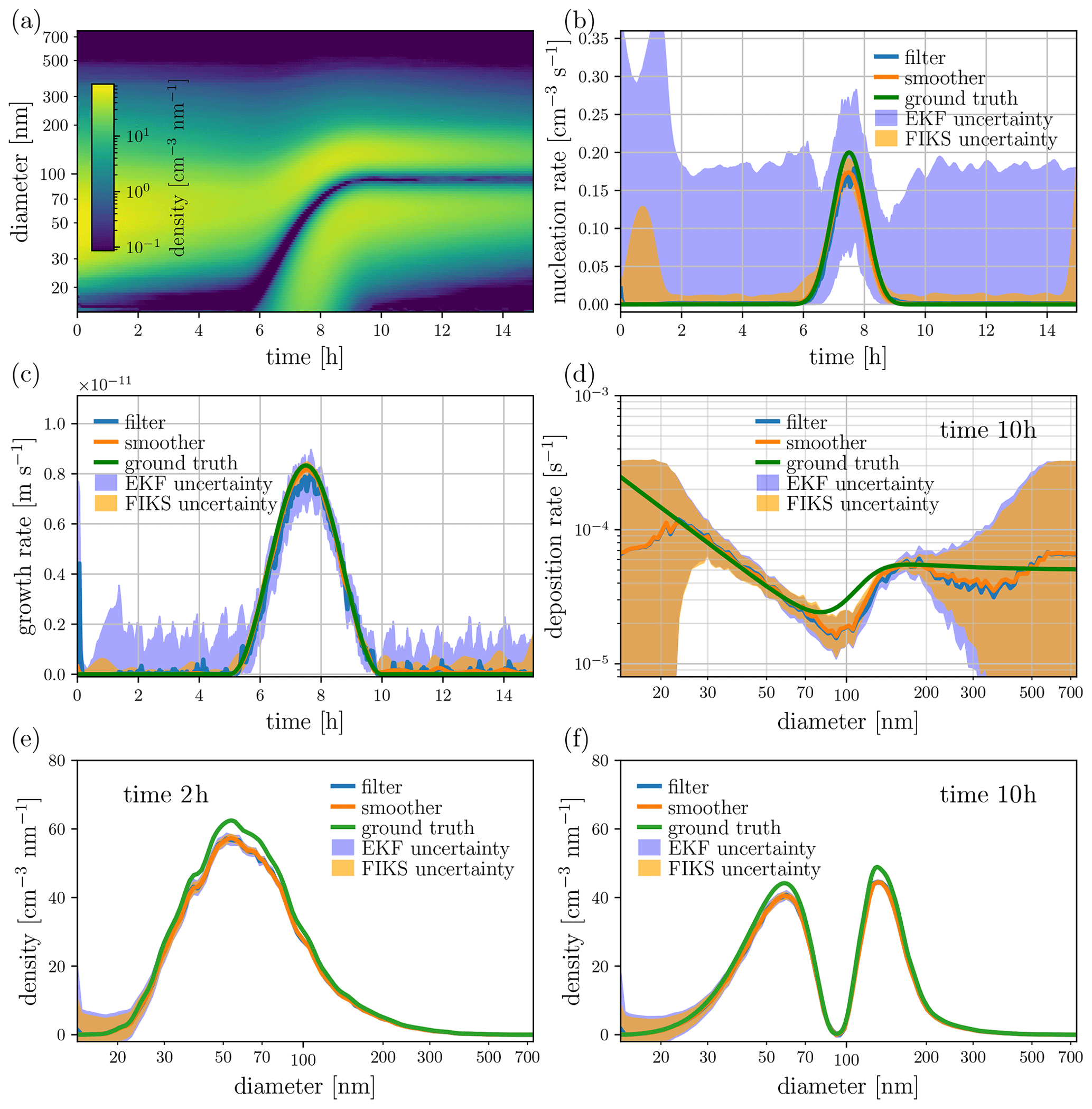
Figure 3Case 1 – NE and high SNR. State estimates for the particle size density (a, e, f), nucleation rate (b), growth rate (c) and loss rate (d). The image in plot (a) depicts the approximate posterior expectation for the entire time-evolution of the particle size density given by FIKS, whereas plots (e) and (f) illustrate the EKF and FIKS estimates corresponding to times 2 and 10 h, respectively. In plots (b)–(f), the blue and orange lines represent the approximate posterior expectations for EKF and FIKS, respectively, and the areas shaded with light blue and orange are the respective posterior error intervals. The true values of the corresponding quantities are drawn with a green line.
The estimated particle size density (Fig. 3a) is in rather good correspondence with the true size density (Fig. 1a). However, the size density estimates corresponding to times 2 and 10 h (Fig. 3e and f, respectively) show that the peak values of the size density are somewhat underestimated by both EKF and FIKS. Moreover, in these instants, the true values of the size density are partly outside the approximate posterior error intervals. Yet the 68 % posterior error intervals do not necessarily need to contain the true values, and the error intervals seem to be slightly too narrow. This underestimation of the uncertainty is due to the linearizations/Gaussian approximation behind EKF and FIKS, as shown by Huttunen et al. (2018), and the rather simple approximations of the error in the evolution and the measurement models – underestimating the covariance in the models. The errors caused by model approximations become more influential with decreasing mean noise level – the remedy for such errors could be the Bayesian approximation error method (Kaipio and Somersalo, 2006); however, this is out of the scope of this paper.
For the process rates, the approximate posterior means given by both EKF and FIKS are relatively close to the true values (Fig. 3b–d). Overall, the FIKS estimates for the process rate parameters are more accurate than the EKF estimates – this is an expected result because FIKS utilizes the entire data set up to the end of the process, whereas EKF only uses data up to time t when estimating the variables at time t.
The filter and smoother also show differences in the posterior error intervals of the process rate parameters: the error intervals given by EKF are systematically wider than those given by FIKS. This is again an expected result because the use of the future data (FIKS) should reduce the uncertainty in the estimated quantities. Furthermore, in almost all instants in time, the process rate parameters (especially growth and apparent particle formation rates) are within the posterior error intervals. This is a desired result, as it indicates that these approximate credible intervals give realistic measures of the estimate uncertainties in these cases.
The loss rate estimate uncertainty depends strongly on the particle size: the posterior error intervals are wide in the lowest and highest size ranges and rather narrow elsewhere. The high uncertainty of the loss factor at the high particle size range dp>400 nm is caused by the lack of data – in this size range, the particle density is nearly zero at all times; consequently, the SMPS data do not provide information on the loss factor. In the lowest size range, the width of the credible interval also depends on time. From time t = 9 h, when the nucleation event is practically over, the particle size density in the lowest size range is almost zero, again resulting in high uncertainty in the loss factor estimate. The loss rate estimate and posterior error interval resulting from the FIKS are virtually time invariant, even though those from the EKF show a strong time dependence.
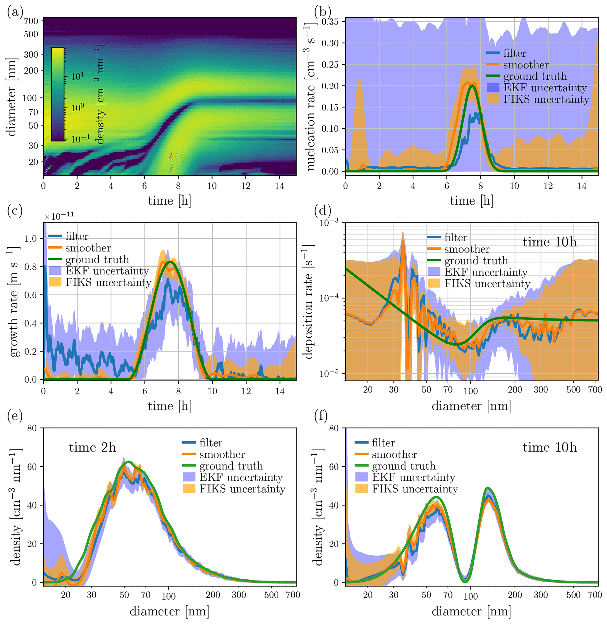
Figure 4Case 2 – NE and low SNR. State estimates for the particle size density (a, e, f), nucleation rate (b), growth rate (c) and loss rate (d). The image in plot (a) depicts the approximate posterior expectation for the entire time-evolution of the particle size density given by FIKS, whereas plots (e) and (f) illustrate the EKF and FIKS estimates corresponding to times 2 and 10 h, respectively. In plots (b)–(f), the blue and orange lines represent the approximate posterior expectations for EKF and FIKS, respectively, and the areas shaded with light blue and orange are the respective posterior error intervals. The true values of the corresponding quantities are drawn with a green line.
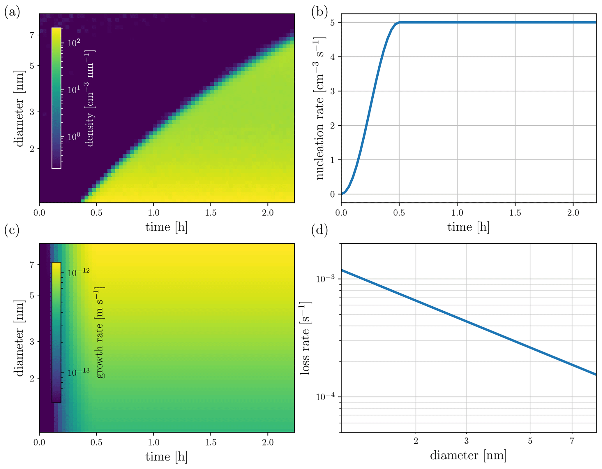
Figure 5Cases 3 and 4 – steady-state system, showing true (simulated) processes: (a) particle size density (measurement), (b) nucleation rate, (c) growth rate and (d) wall loss rate.
In Case 1, the SNR is high, and – apart from the aforementioned exceptions – the estimate uncertainty is very low. Figure 4 shows the results of Case 2, where the SNR is significantly lower. As expected, the process rate estimates become less accurate than in Case 1. However, the change in the accuracy is quite small, especially for FIKS – demonstrating that the Kalman smoother estimates tolerate measurement noise rather well. As expected, the posterior error intervals of all estimated quantities are clearly wider than in the case of high SNR – this is a result of increased uncertainty in the particle counter observations. Both EKF and FIKS lead to safe posterior error intervals for the process rate parameters, and FIKS again gives clearly narrower posterior error intervals than EKF. The true values of the process rate parameters are once again within the posterior error intervals, further confirming the feasibility of Bayesian state estimation for quantifying the uncertainties of the process rates.
One may notice the appearance of spurious oscillations in the size distribution at low sizes during the particle formation event in Case 2 (Fig. 4a), which were completely smoothed out in Case 1 (Fig. 3a). These oscillations are due to the instability of Eqs. (5) and (6) which are corrected during the estimation by the assimilation of the data. However, while the data in Case 1 allow for the estimates to be neatly rectified, the data in Case 2 cannot completely make up for the instability. Note that the tolerance with respect to such modeling errors (e.g., discretization) can be further improved by so-called approximation error analysis (Huttunen and Kaipio, 2007).
3.2 Cases 3 and 4: steady state (SS)
3.2.1 SS: data simulation and parameter estimation
In the SS simulations in this paper, the condensation rate is both size dependent and time dependent, and the wall loss rate is time invariant but depends on size. Both the nucleation and condensation rates start from zero and grow within the first 30 min until they reach their stationary values. In such a case, the new particle formation and condensational growth are compensated for by wall losses, leading to the number concentration function to reach a steady state. The simulated process rates and the particle size density are illustrated in Fig. 5. Here, the size range of particles is [0.87 nm, 10.00 nm], and it is discretized into Q=1731 logarithmically distributed bins. Note that the value is most certainly below any physically relevant critical sizes; however, from a simulation stand point, any size range could have been utilized to simulate a similar chamber experiment, only the values of the parameters would require adjustments.
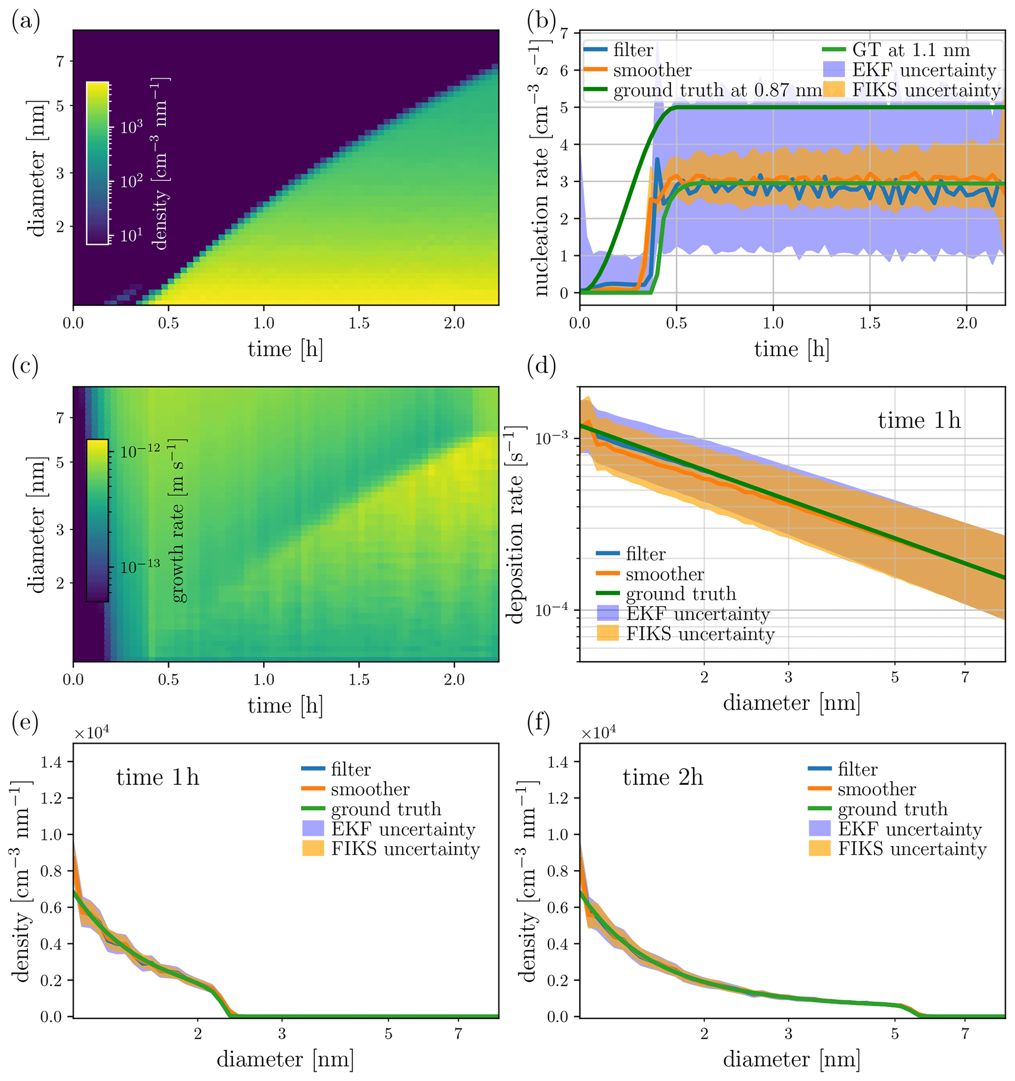
Figure 6Case 3 – SS, high SNR. State estimates for the particle size density (a, e, f), nucleation rate (b), growth rate (c) and wall loss rate (d). The images in plots (a) and (c) depict the approximate, FIKS-based posterior expectations for the entire time-evolution of the corresponding quantities. Plots (e) and (f) illustrate the EKF and FIKS estimates for the particle size density corresponding to times 1 and 2 h, respectively. In plots (b) and (d–f), the blue and orange lines represent the approximate posterior expectations for EKF and FIKS, respectively, and the areas shaded with light blue and orange are the respective posterior error intervals. The true values of the corresponding quantities are drawn with a green line.
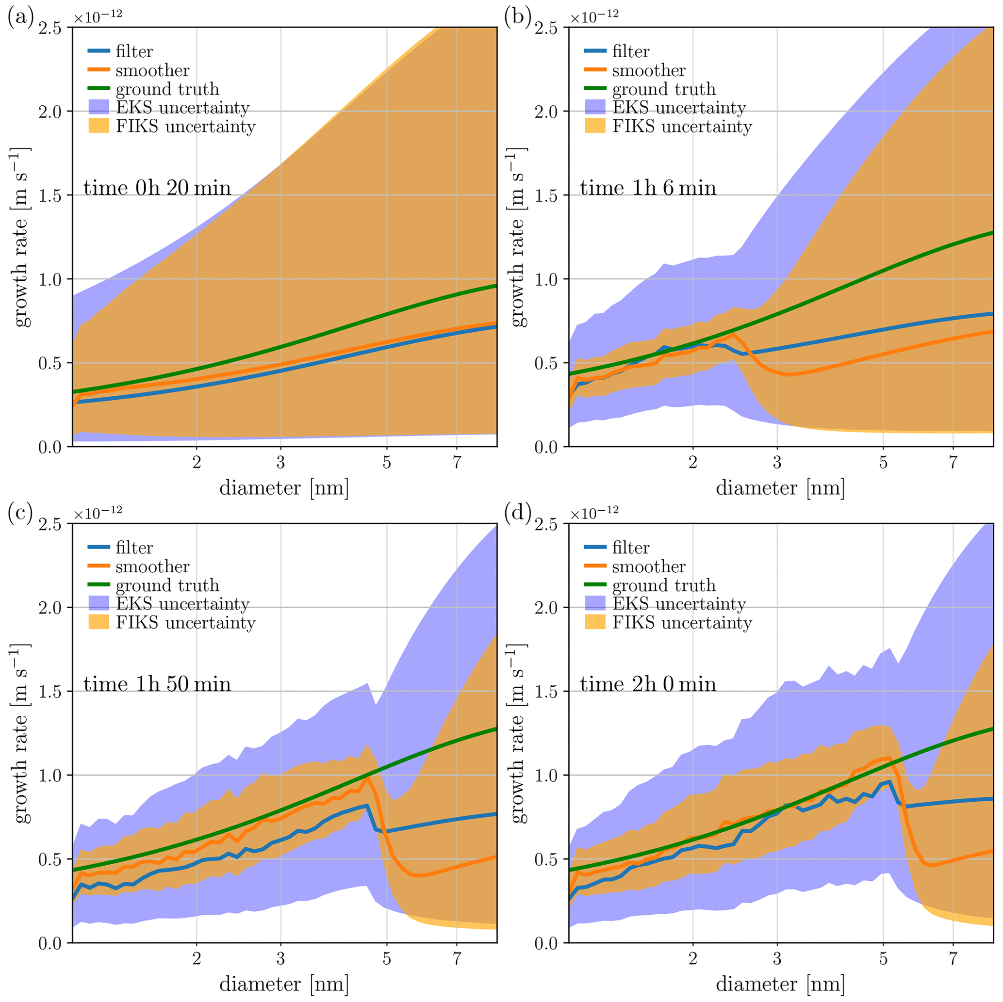
Figure 7Case 3 – SS and high SNR. Condensational growth rate estimates corresponding to four instants in time. The blue and orange lines represent the approximate posterior expectations for EKF and FIKS, respectively, and the areas shaded with light blue and orange are the respective posterior error intervals. The true growth rates are marked with green lines.
The synthetic SMPS data are simulated similarly to cases 1 and 2. Again, two cases corresponding to different SNRs are simulated by generating the Poisson-distributed observations corresponding to two sample volumes: V=200 cm3 (Case 3: SS, high SNR) and V=2 cm3 (Case 4: SS, low SNR). In Case 3, the range of SNR was [0,4440]; in Case 4 it was [0,44.4].
In the state space, the lower end of the size discretization bin (i.e., Ω1 in Sect. 2.1.1) is centered at 1.1 nm (its lower boundary is about 1.08 nm). Many potential bins would separate the critical size from the lower end of the state space . The reason that we are not setting is because, with the current technology, it is not realistic to assume that we can acquire reliable data down to the critical size. Note that it is possible, however, to extend the model down to the critical size in order to estimate the true nucleation rate – provided that the GDE is still valid for such small particles. However, without measurement from the lower end of the spectrum, the uncertainty will overwhelm the estimates, rendering them non-informative. This extension is outside of the scope of this paper.
The time evolution of the apparent particle formation and growth rates are modeled as second-order Markov processes (Eq. 12), whereas the wall loss rates are modeled as first-order Markov processes (Eq. 11). The growth and wall loss rates are assumed to be smooth with respect to size; hence, the state noises in the corresponding evolution models are modeled as correlated. For details of the model choices, we refer to Appendix B.
3.2.2 SS: results and discussion
Figure 6 illustrates the estimates of the particle size density and process rates in the case of high SNR (Case 3). For the particle size density and condensation rate, the respective images in Fig. 6a and c show the approximate FIKS-based posterior means of those time- and size-dependent variables. For the nucleation rate as well as for the instantaneous wall loss rate and size densities, both the filter and smoother estimates (approximate posterior expectations and error intervals) are plotted.
In this case, the smoother estimate for the particle size density is in very good correspondence with the true density (see Fig. 5a). Further, the uncertainty estimates for the particle size density are feasible: the true size density lies within the posterior error intervals given by EKF and FIKS.
The apparent particle formation rate is well estimated by both the EKF and the FIKS; the true value lies within the posterior error intervals most of the time. Only at the onset of the appearance of particles into the measured size range does the true value not lie within the uncertainty range, around t=25 min. Similarly to the NE cases, the FIKS estimates are less uncertain than those from the EKF, and the SNR levels are a major factor determining the accuracy of the estimates: the higher the SNR, the better the estimate. While the true nucleation rate plotted in dark green takes place at 0.87 nm, in the state-space model, the diameter that corresponds to the apparent particle formation, plotted in light green, is about 1.08 nm (the lower end of the smallest size bin, geometrical center at 1.1 nm). This difference between the model used for simulating the data and the model used in estimation causes the systematic error – underestimation of the nucleation rate.
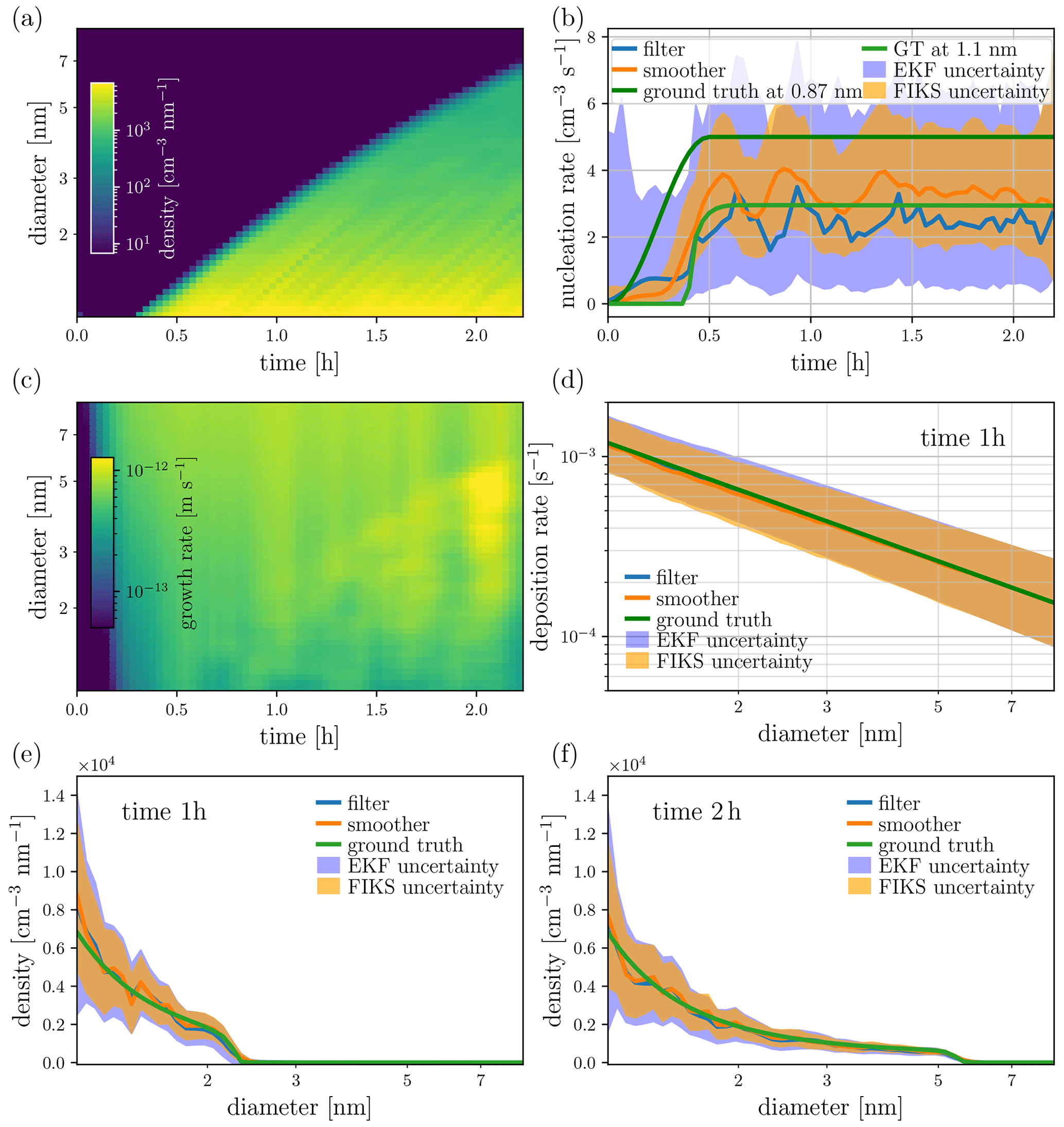
Figure 8Case 4 – SS and low SNR. State estimates for the particle size density (a, e, f), nucleation rate (b), growth rate (c) and wall loss rate (d). The images in plots (a) and (c) depict the approximate, FIKS-based posterior expectations for the entire time-evolution of the corresponding quantities. Plots (e) and (f) illustrate the EKF and FIKS estimates for the particle size density corresponding to times 1 and 2 h, respectively. In plots (b) and (d–f), the blue and orange lines represent the approximate posterior expectations for EKF and FIKS, respectively, and the areas shaded with light blue and orange are the respective posterior error intervals. The true values of the corresponding quantities are drawn with a green line.
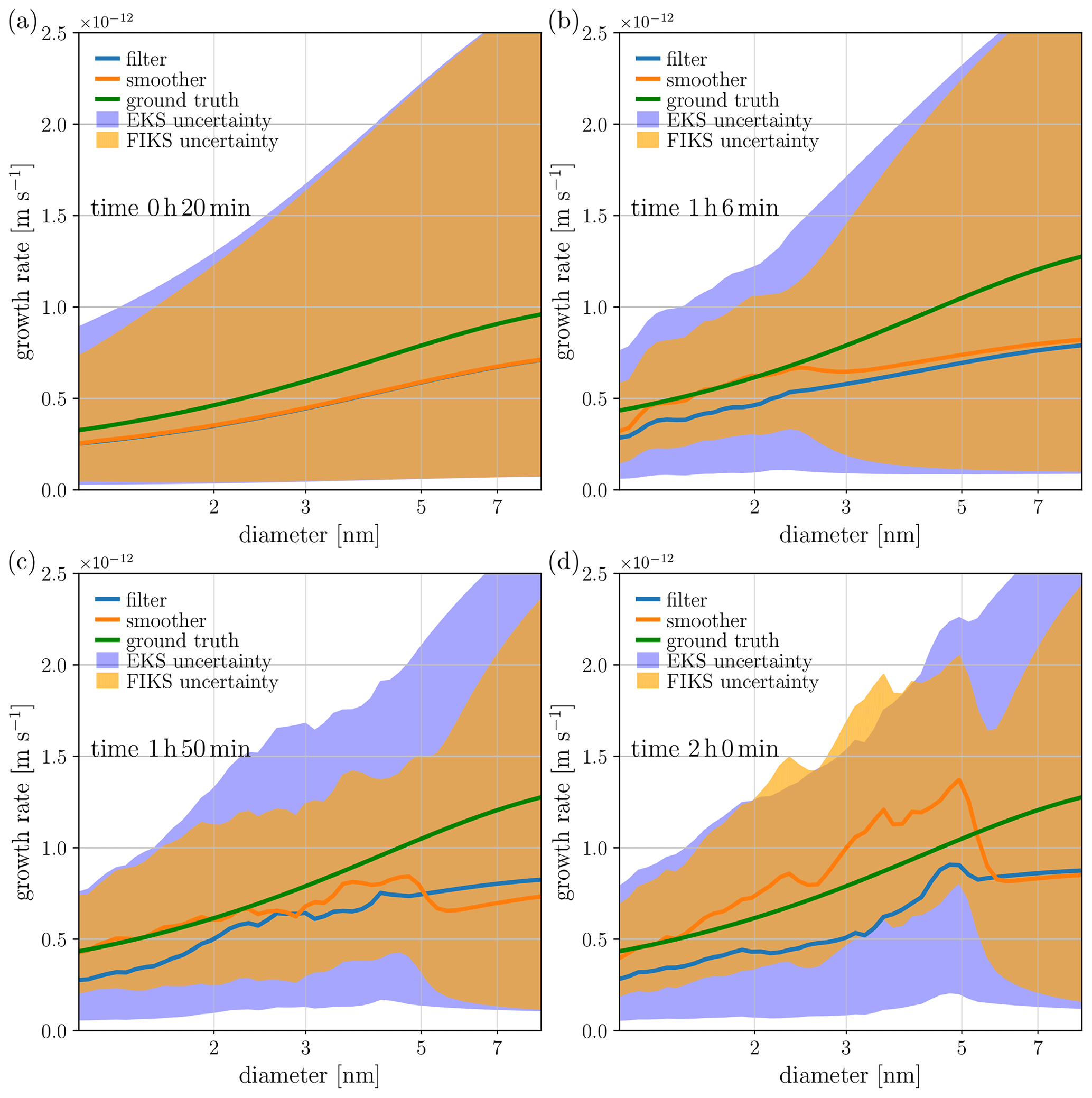
Figure 9Case 4 – SS and low SNR. Condensational growth rate estimates corresponding to four instants in time. The blue and orange lines represent the approximate posterior expectations for EKF and FIKS, respectively, and the areas shaded with light blue and orange are the respective posterior error intervals. The true growth rates are marked with green lines.
Figure 6c shows a clear trend in the quality of the smoother estimate for the condensational growth rate: at an early stage of the process (time ∼0.25 h), FIKS infers the growth rate reliably only in the smallest size classes (diameter ∼1 nm); in the larger particle sizes, the growth rate is heavily underestimated (see Fig. 5c). As time progresses, the growth rate estimates become gradually more reliable in larger and larger size classes.
The gradual improvement in the growth rate estimates in the larger size classes is a direct consequence of the propagation of the particle number density towards large size classes. Indeed, comparison of Fig. 6a and c reveals that the size class where FIKS catches the increase in the growth rate parameter (light/yellow area in the condensation rate image Fig. 6c) follows accurately the propagating front of the number density in Fig. 6a. The reason for this property of the growth rate estimate is obvious: in the size classes where the particle number density is very low, the measurement data do not carry information on the growth rate parameters. In the beginning of the process, the particle number density is low in all classes. When nucleation starts producing particles to the smallest size class and these particles grow, the growth is sensed by the particle size analyzer measurements. When the particle sizes keep increasing due to condensation, the measurements corresponding to increasingly larger size classes become sensitive to the process rate parameters.
Figure 7 illustrates the EKF and FIKS estimates of the growth rate corresponding to four instants in time. These plots confirm the above discussion on the growth rate estimation: at time 1 h and 6 min, both the EKF- and FIKS-based posterior means underestimate the growth rate in the large size classes (above ∼2.5 nm), and for the subsequent times, the EKF and especially FIKS estimates become reliable in gradually increasing size classes. Furthermore, Fig. 7 shows a trend in the evolution of the posterior error intervals of the growth rate: at time 1 h and 6 min, the posterior error intervals are really wide in classes >2.5 nm, reflecting high uncertainty in the growth rate estimates in this size range. As time progresses, the size range of low uncertainty spreads towards large size classes. This result demonstrates that Bayesian filtering and smoothing yield feasible posterior error estimates – indicating high uncertainty in the size ranges where the posterior expectations are unreliable in this example.
The EKF estimates of the growth rate in Fig. 7 show similar behavior to the FIKS estimates; the main differences are that, as expected, the posterior means given by EKF are more biased than those in FIKS, and the posterior error intervals are generally wider than with FIKS.
Figures 8 and 9 show the results of Case 4 – SS and low SNR data. The properties of the state estimates are very similar to those in Case 3, except for the anticipated differences: the lower accuracy of the approximate posterior means, and wider posterior error intervals – again indicating the increase in the uncertainty when the SNR of the measurements gets lower.
The radiative forcing caused by aerosols – and the underlying processes of new particle formation and growth – are currently understood to be the most uncertain factors in the prediction of climate change. While a significant effort has been directed into experimental campaigns for collecting data that carry indirect information on these processes and their effects, computational methods for analyzing the data are still insufficient for reliable estimation of the process rates.
In this paper, the problem of estimating the apparent particle formation, growth and loss rates of aerosols was cast in the framework of Bayesian state estimation. We modeled the dynamics of aerosol size distributions with the general dynamics equation and considered the (process rate) parameters in the model as unknown state variables. These size- and/or time-dependent variables were estimated together with the particle number density based on sequential particle counter measurements using the extended Kalman filter (EKF) and fixed interval Kalman smoother (FIKS). Furthermore, to quantify the uncertainties of the estimated variables, we also computed posterior error intervals for the process rate parameters.
The approach was tested with a set of numerical simulation studies, where two processes of different types were considered: (1) a nucleation event, which qualitatively represents a typical particle formation event in the atmosphere, and (2) a process approaching steady state, which is representative of a particle formation and growth in a chamber experiment. The EKF- and especially FIKS-based estimates for the process rates were generally reliable, even in cases of low SNR data. Moreover, the posterior error intervals were feasible – that is, the true process rates lie mostly within the approximate error intervals. The reason why FIKS estimates are generally superior to EKF estimates is that Bayesian smoothers also use future data when estimating a quantity at given time t, whereas filter estimates are based on only the data up to the point t. In online and control applications, of course, the future data are not available; however, in the applications targeted in this paper, the data analysis is done after the experiment – that is, the entire data set is available for Bayesian smoothing. The results of the numerical studies support the feasibility of the proposed approach to estimating the aerosol formation, growth and deposition rates, and quantifying their uncertainties. Based on these findings, we conclude that Bayesian state estimation (combined with aerosol particle dynamics modeling) offers a reliable tool for analyzing sequentially measured particle counter data. The estimated aerosol process rates and their uncertainties can improve the analysis of the experimental data and provide better insight on the particle formation and growth in the atmosphere. In the future, such analysis can potentially offer improved assessment of the radiative forcing by aerosols and its uncertainty. Eventually, this can lead to improved predictions and uncertainty quantification of the climate change via a combination of the enhanced process rate estimates and their uncertainties with global aerosol–climate models.
Table A1Summary of the models and parameters used for simulating data in nucleation event (NE) and steady-state (SS) cases. Here, the growth rate g is assumed to be a product of a size- and time-dependent parts – that is, g=gd(dp)gt(dt). “evol.” denotes “evolution”, and “obs.” represents “observed”.
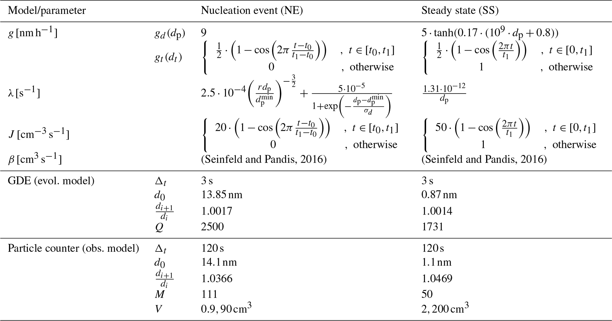
Table A1 lists the models and parameters used for simulating the nucleation, condensation and deposition processes, and the particle size density, as well as modeling the particle counter data.
Table B1Qualitative description of the models used in state estimation for nucleation event (NE) and steady-state (SS) cases.
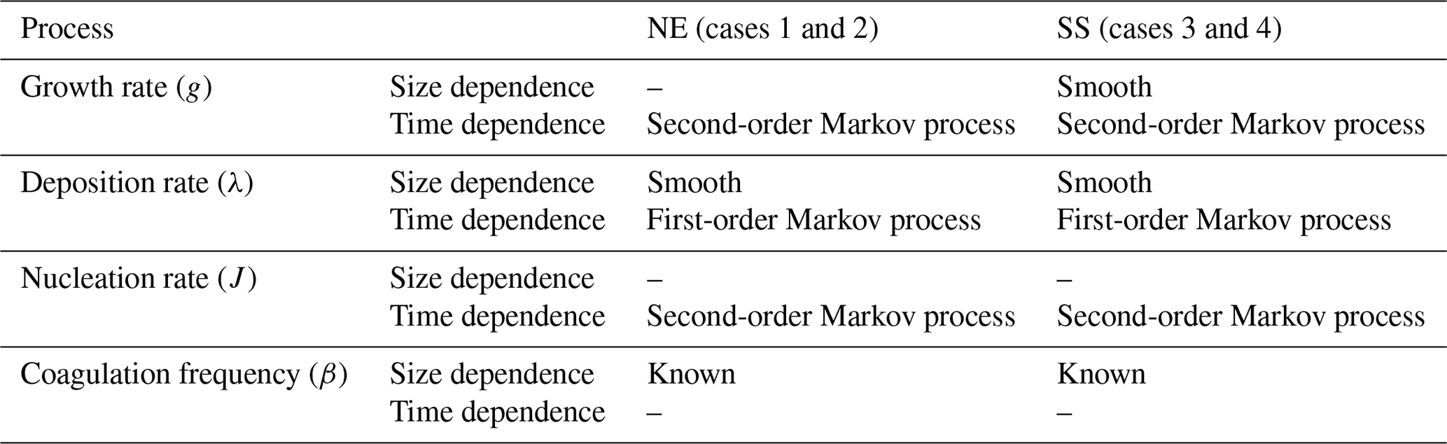

Figure B1Covariance matrices of (a) the deposition rate λ in cases 1 and 2 and (b)
growth rate g in cases 3 and 4.
In this Appendix, we describe the choices of models and parameters made for state estimation in the numerical examples (Sect. 3). We start by qualitatively summarizing the choices of models for the process rates in the two example cases, a nucleation event (NE) and steady state (SS), see Table B1.
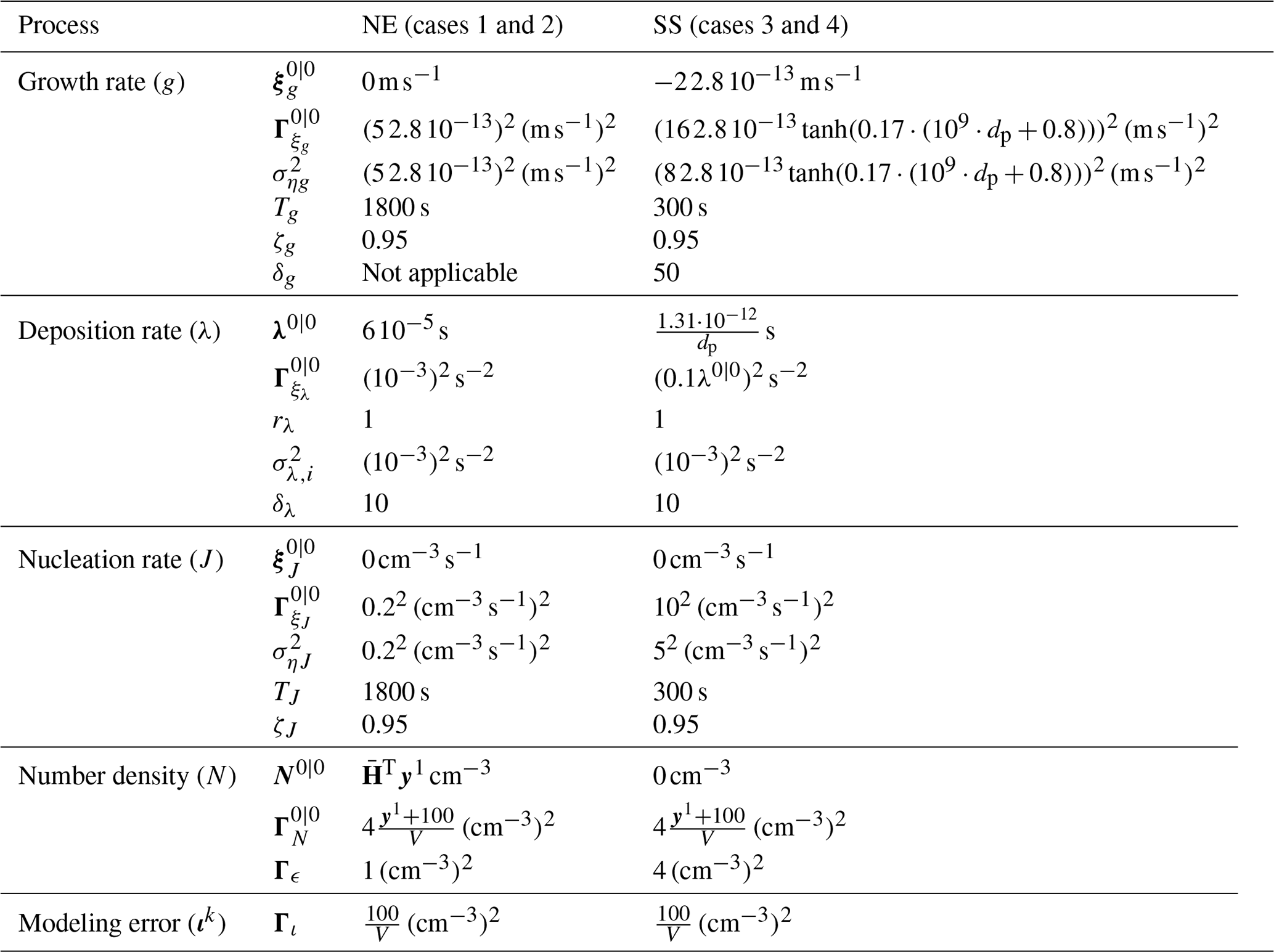
Table B2Parameters used in state estimation for nucleation event (NE) and steady-state (SS) cases.
In the following, we first describe how the smoothness of the size-dependent parameters is formulated. Next, we discuss modeling the time dependence of the parameters by first- and second-order Markov models. Finally, we list all parameter values chosen for each test case.
B1 Size-dependent processes: smoothness
The size-dependent process rate variables – loss rate (λ) in all test cases and the growth rate (g) in the SS cases – are assumed to be smooth functions of size. As these variables also depend on time, we model them as multivariate stochastic processes, particularly first-order Markov processes, as described below. The smoothness in size is accounted for by modeling elements of each of the associated random variables (size-discretized process rate variables , ) at a given time k as mutually correlated.
where is the variance of , and δφ is a parameter defining how steeply the cross-covariance between elements and decreases as a function of the difference between indices i and j.
Figure B1 shows the covariance matrices of the two size-dependent variables: loss rate (λ) in cases 1 and 2 and growth rate (g) in cases 3 and 4. We note here that is constant in cases 1 and 2, whereas increases with particle size in cases 3 and 4. Details of parameter values are given in the following.
B2 Time-dependence: first-order Markov processes
Assume next that the process rate variable is modeled as a first-order Markov process. Here, we fix the covariance of first, as well as the temporal smoothness (first- or second-order Markov process). We then determine the covariance of the driving noise process.
When the covariance matrix of is time invariant, we can calculate the covariance matrix of the state noise using Eq. (11) as follows:
In cases of size-dependent variables, we construct the covariance matrix as described above, fix the state transition matrix Ψφ=rφI, by choosing the parameter , and, finally, compute the state noise covariance matrix using Eq. (B2). Note, however, that in the case of a scalar variable modeled as a first-order Markov process φ, which does not depend on size, the state-transition matrix and the covariance are simply Ψφ=rφ and , respectively.
B3 Time-dependence: second-order Markov processes
As shown in Table B1, the size-independent variables in cases 1 and 2 (g and J) are modeled as second-order Markov processes. For these variables, we choose the root parameters and in the evolution models using an approach adopted from the analysis of second-order systems, such as damped oscillators. We first define a characteristic time is Tφ and damping ratio ζφ, and then calculate and by solving the set of equations:
These parameters, along with separately chosen variances of the state noises and as well as the expectations and variances of the initial states and , define the properties of the second-order Markov models.
B4 Parameter choices
All parameter values chosen for state estimation in each test case are listed in Table B2.
The current version of the code used to generate the data as well as the implementation of the estimation method are available under the MIT Expat License at https://doi.org/10.5281/zenodo.4061728 (Ozon, 2020). The exact version of the code used to produce the results in this paper will be the initial version of the code.
The state-space formulation of the aerosol process rate estimation problem was contributed by all authors. MO implemented all software used in the computations. The numerical experiments were planned and analyzed by all authors. All authors took active part in writing the paper.
The authors declare that they have no conflict of interest.
The authors wish to thank the reviewers for their comments on the paper.
This research has been supported by the Academy of Finland (grant nos. 325647 and 337550) and by the Center of Excellence on Inverse Modelling and Imaging (grant nos. 336795 and 336790).
This paper was edited by Christina McCluskey and reviewed by two anonymous referees.
Ackleh, A.: Parameter estimation in a structured algal coagulation-fragmentation model, Nonlinear Anal., 28, 837–854, https://doi.org/10.1016/0362-546X(95)00195-2, 1997. a
Ackleh, A. S. and Miller, R. L.: A model for the interaction of phytoplankton aggregates and the environment: approximation and parameter estimation, Inverse Probl. Sci. En., 26, 152–182, https://doi.org/10.1080/17415977.2017.1310856, 2018. a
Aitken, J.: On the Number of Dust Particles in the Atmosphere, T. Roy. Soc. Edin.-Earth, 35, 1–19, https://doi.org/10.1017/S0080456800017592, 1889. a
Almeida, J., Schobesberger, S., Kürten, A., Ortega, I. K., Kupiainen-Määttä, O., Praplan, A. P., Adamov, A., Amorim, A., Bianchi, F., Breitenlechner, M., David, A., Dommen, J., Donahue, N. M., Downard, A., Dunne, E., Duplissy, J., Ehrhart, S., Flagan, R. C., Franchin, A., Guida, R., Hakala, J., Hansel, A., Heinritzi, M., Henschel, H., Jokinen, T., Junninen, H., Kajos, M., Kangasluoma, J., Keskinen, H., Kupc, A., Kurtén, T., Kvashin,A. N., Laaksonen, A., Lehtipalo, K., Leiminger, M., Leppä,J., Loukonen, V., Makhmutov, V., Mathot, S., McGrath, M. J., Nieminen, T., Olenius, T., Onnela, A., Petäjä, T., Riccobono, F., Riipinen, I., Rissanen, M., Rondo, L., Ruuskanen, T., Santos, F. D., Sarnela, N., Schallhart, S., Schnitzhofer, R., Seinfeld, J. H., Simon, M., Sipilä, M., Stozhkov, Y., Stratmann, F., Tomé, A., Tröstl, J., Tsagkogeorgas, G., Vaattovaara, P., Viisanen, Y., Vir-tanen, A., Vrtala, A., Wagner, P. E., Weingartner, E., Wex, H., Williamson, C., Wimmer, D., Ye, P., Yli-Juuti, T., Carslaw, K. S., Kulmala, M., Curtius, J., Baltensperger, U., Worsnop, D. R.,Vehkamäki, H., and Kirkby, J.: Molecular understanding of sulphuric acid-amine particle nucleation in the atmosphere, Nature, 502, 359–363, https://doi.org/10.1038/nature12663, 2013. a
Banks, H., Tran, H., and Woodward, D.: Estimation of Variable Cefficients in the Fokker–Planck Quations Using Moving Node Finite Elements, SIAM J. Numer. Anal., 30, 1574–1602, https://doi.org/10.1137/0730082, 1993. a
Boisdron, Y. and Brock, J.: On the stochastic nature of the acquisition of electrical charge and radioactivity by aerosol particles, Atmos. Environ., 4, 35–50, 1970. a
Bortz, D., Byrne, E., and Mirzaev, I.: Inverse Problems for a Class of Conditional Probability Measure-Dependent Evolution Equations, arXiv preprint, arXiv:1510.01355, 2015. a
Cho, C.-K. and Kwon, Y.: Parameter Estimation for Age-Structured Population Dynamics, Journal of the Korean Society for Industrial and Applied Mathematics, 1, 83–104, available at: https://www.koreascience.or.kr/article/JAKO199725051942749.pdf (last access: 18 July 2017), 1997. a
Courant, R., Friedrichs, K., and Lewy, H.: Über die partiellen Differenzengleichungen der mathematischen Physik, Math. Ann., 100, 32–74, https://doi.org/10.1007/BF01448839, 1928. a
Dada, L., Lehtipalo, K., Kontkanen, J., Nieminen, T., Baalbaki, R., Ahonen, L., Duplissy, J., Yan, C., Chu, B., Petäjä, T., Lehtinen, K., Kerminen, V.-M., Kulmala, M., and Kangasluoma, J.: Formation and growth of sub-3-nm aerosol particles in experimental chambers, Nat. Protoc., 15, 1013–1040, 2020. a, b
Dimitriu, G.: Parameter estimation in size/age structured population models using the moving finite element method, in: International Conference on Numerical Methods and Applications, edited by: Dimov, I., Lirkov, I., Margenov, S., and Zlatev, Z., Numerical Methods and Applications, NMA 2002, Lecture Notes in Computer Science, vol. 2542, Springer, Berlin, Heidelberg, 420–429, https://doi.org/10.1007/3-540-36487-0_47, 2002. a
Dugas, C., Bengio, Y., Bélisle, F., Nadeau, C., and Garcia, R.: Incorporating second-order functional knowledge for better option pricing, in: Advances in neural information processing systems, 472–478, available at: http://papers.nips.cc/paper/1920-incorporating-second-order-functional-knowledge-for-better-option-pricing.pdf (last access: May 2002), 2001. a
Dullemond, C. and Dominik, C.: Dust coagulation in protoplanetary disks: A rapid depletion of small grains, Astron. Astrophys., 434, 971–986, https://doi.org/10.1051/0004-6361:20042080, 2005. a
Flagan, R.: History of electrical aerosol measurements, Aerosol Sci. Tech., 28, 301–380, 1998. a
Friedlander, S. and Wang, C.: The self-preserving particle size distribution for coagulation by Brownian motion, J. Colloid Interf. Sci., 22, 126–132, https://doi.org/10.1016/0021-9797(66)90073-7, 1966. a
Gelb, A.: Applied optimal estimation, MIT press, available at: http://users.isr.ist.utl.pt/~pjcro/temp/Applied%20Optimal%20Estimation%20-%20Gelb.pdf (last access: 15 June 2021), 1974. a, b, c, d, e
Gordon, H., Sengupta, K., Rap, A., Duplissy, J., Frege, C., Williamson, C., Heinritzi, M., Simon, M., Yan, C., Almeida, J., Tröstl, J., Nieminen, T., Ortega, I. K., Wagner, R., Dunne, E. M., Adamov, A., Amorim, A., Bernhammer, A.-K., Bianchi, F., Breitenlechner, M., Brilke, S., Chen, X., Craven, J. S., Dias, A., Ehrhart, S., Fischer, L., Flagan, R. C., Franchin, A., Fuchs, C., Guida, R., Hakala, J., Hoyle, C. R., Jokinen, T., Junninen, H., Kangasluoma, J., Kim, J., Kirkby, J., Krapf, M., Kürten, A., Laaksonen, A., Lehtipalo, K., Makhmutov, V., Mathot, S., Molteni, U., Monks, S. A., Onnela, A., Peräkylä, O., Piel, F., Petäjä, T., Praplan, A. P., Pringle, K. J., Richards, N. A. D., Rissanen, M. P., Rondo, L., Sarnela, N., Schobesberger, S., Scott, C. E., Seinfeld, J. H., Sharma, S., Sipilä, M., Steiner, G., Stozhkov, Y., Stratmann, F., Tomé, A., Virtanen, A., Vogel, A. L., Wagner, A. C., Wagner, P. E., Weingartner, E., Wimmer, D., Winkler, P. M., Ye, P., Zhang, X., Hansel, A., Dommen, J., Donahue, N. M., Worsnop, D. R., Baltensperger, U., Kulmala, M., Curtius, J., and Carslaw, K. S.: Reduced Anthropogenic Aerosol Radiative Forcing Caused by Biogenic New Particle Formation, P. Natl. Acad. Sci. USA, 113, 12053–12058, https://doi.org/10.1073/pnas.1602360113, 2016. a
Hansen, J., Johnson, D., Lacis, A., Lebedeff, S., Lee, P., Rind, D., and Russell, G.: Climate impact of increasing atmospheric carbon dioxide, Science, 213, 957–966, 1981. a
Henze, D., Seinfeld, J., Liao, W., Sandu, A., and Carmichael, G.: Inverse modeling of aerosol dynamics: Condensational growth, J. Geophys. Res.-Atmos., 109, D14201, https://doi.org/10.1029/2004JD004593, 2004. a
Huttunen, J., Kaipio, J., and Haario, H.: Approximation error approach in spatiotemporally chaotic models with application to Kuramoto–Sivashinsky equation, Comput. Stat. Data An., 123, 13–31, https://doi.org/10.1016/j.csda.2018.01.015, 2018. a
Huttunen, J. M. J. and Kaipio, J. P.: Approximation error analysis in nonlinear state estimation with an application to state-space identification, Inverse Probl., 23, 2141–2157, https://doi.org/10.1088/0266-5611/23/5/019, 2007. a
Kaipio, J. and Somersalo, E.: Statistical and computational inverse problems, Vol. 160, Springer Science and Business Media, Springer, New York, NY, https://doi.org/10.1007/b138659, 2006. a, b, c, d
Kalman, R.: A New Approach to Linear Filtering and Prediction Problems, J. Basic Eng.-T. ASME, 82, 35–45, https://doi.org/10.1115/1.3662552, 1960. a
Kirkby, J., Duplissy, J., Sengupta, K., Frege, C., Gordon, H. Williamson, C., Heinritzi, M., Simon, M., Yan, C., Almeida, J., Tröstl, J., Nieminen, Ortega, T., Wagner, R., Adamov, A., Amorim, A., Bernhammer, A., Bianchi, F., Breitenlechner, M., Brilke, S., Chen, X., Craven, J., Dias, A., Ehrhart, S., Flagan, R. C., Franchin, A., Fuchs, C., Guida, R., Hakala, J., Hoyle, C. R., Jokinen, T., Junninen, H. Kangasluoma, J., Kim, J., Krapf, M. Kürten, A., Laaksonen, A., Lehtipalo, K., Makhmutov, V., Mathot, S., Molteni, U., Onnela, A., Peräkylä, O., Piel, F., Petäjä, T., Praplan, A. P., Pringle, K., Rap, A., Richards, N., Riipinen, I., Rissanen, M. P., Rondo, L., Sarnela, N., Schobesberger, S., Scott, C., Seinfeld, J. H., Sipilä, M., Steiner, G., Stozhkov, Y., Stratmann, F., Tomé, A., Virtanen, A., Vogel, A., Wagner, A., Wagner, P., Weingartner, E., Wimmer, D., Winkler, P., Ye, P., Zhang, X., Hansel, A., Dommen, J., Donahue, N. M., Worsnop, D., Baltensperger, U., Kulmala, M., Carslaw, K. S., and Curtius, J.: Ion-Induced Nucleation of Pure Biogenic Particles, Nature, 476, 429–433, https://doi.org/0.1038/nature17953, 2016. a
Korhonen, H., Lehtinen, K. E. J., and Kulmala, M.: Multicomponent aerosol dynamics model UHMA: model development and validation, Atmos. Chem. Phys., 4, 757–771, https://doi.org/10.5194/acp-4-757-2004, 2004. a
Kuang, C., Chen, M., Zhao, J., Smith, J., McMurry, P. H., and Wang, J.: Size and time-resolved growth rate measurements of 1 to 5 nm freshly formed atmospheric nuclei, Atmos. Chem. Phys., 12, 3573–3589, https://doi.org/10.5194/acp-12-3573-2012, 2012. a
Kürten, A., Li, C., Bianchi, F., Curtius, J., Dias, A., Donahue, N. M., Duplissy, J., Flagan, R. C., Hakala, J., Jokinen, T., Kirkby, J., Kulmala, M., Laaksonen, A., Lehtipalo, K., Makhmutov, V., Onnela, A., Rissanen, M. P., Simon, M., Sipilä, M., Stozhkov, Y., Tröstl, J., Ye, P., and McMurry, P. H.: New particle formation in the sulfuric aciddimethylaminewater system: reevaluation of CLOUD chamber measurements and comparison to an aerosol nucleation and growth model, Atmos. Chem. Phys., 18, 845–863, https://doi.org/10.5194/acp-18-845-2018, 2018. a
Kulmala, M., Vehkamäki, H., Petäjä, T., Maso, M. D., Lauri, A., Kerminen, V.-M., Birmili, W., and McMurry, P.: Formation and growth rates of ultrafine atmospheric particles: a review of observations, J. Aerosol Sci., 35, 143–176, https://doi.org/10.1016/j.jaerosci.2003.10.003, 2004. a
Kulmala, M., Petäjä, T., Nieminen, T., Sipilä, M., Manninen, H., Lehtipalo, K., Maso, M. D., Aalto, P., Junninen, H., Paasonen, P., Riipinen, I., Lehtinen, K., Laaksonen, A., and Kerminen, V.-M.: Measurement of the nucleation of atmospheric aerosol particles, Nat. Protoc., 7, 1651, https://doi.org/10.1038/nprot.2012.091, 2012. a, b
Kupiainen-Määttä, O.: A Monte Carlo approach for determining cluster evaporation rates from concentration measurements, Atmos. Chem. Phys., 16, 14585–14598, https://doi.org/10.5194/acp-16-14585-2016, 2016. a
Lehtinen, K. E. J. and Kulmala, M.: A model for particle formation and growth in the atmosphere with molecular resolution in size, Atmos. Chem. Phys., 3, 251–257, https://doi.org/10.5194/acp-3-251-2003, 2003. a
Lehtinen, K. and Zachariah, M.: Self-preserving theory for the volume distribution of particles undergoing Brownian coagulation, J. Colloid Interf. Sci., 242, 314–318, https://doi.org/10.1006/jcis.2001.7791, 2001. a, b
Lehtinen, K., Rannik, Ü., Petäjä, T., Kulmala, M., and Hari, P.: Nucleation rate and vapor concentration estimations using a least squares aerosol dynamics method, J. Geophys. Res.-Atmos., 109, 521–526, https://doi.org/10.1038/nature17953, 2004. a
Lehtinen, K. E., Dal Maso, M., Kulmala, M., and Kerminen, V.-M.: Estimating nucleation rates from apparent particle formation rates and vice versa: Revised formulation of the Kerminen–Kulmala equation, J. Aerosol Sci., 38, 988–994, https://doi.org/10.1016/j.jaerosci.2007.06.009, 2007. a
Lehtipalo, K., Leppä, J., Kontkanen, J., Kangasluoma, J., Franchin, A., Wimmer, D., Schobesberger, S., Junninen, H., Petäjä, T., Sipilä, M., Mikkilä, J., Vanhanen, J., Worsnop, D. R., and Kulmala, M.: Methods for determining particle size distribution and growth rates between 1 and 3 nm using the Particle Size Magnifier, Boreal Environ. Res., 19, 215–236, http://hdl.handle.net/10138/228762 (last access: 15 June 2021), 2014. a, b
Leppä, J., Anttila, T., Kerminen, V.-M., Kulmala, M., and Lehtinen, K. E. J.: Atmospheric new particle formation: real and apparent growth of neutral and charged particles, Atmos. Chem. Phys., 11, 4939–4955, https://doi.org/10.5194/acp-11-4939-2011, 2011. a
Maso, M. D., Kulmala, M., Riipinen, I., Wagner, R., Hussein, T., Aalto, P., and Lehtinen, K.: Formation and growth of fresh atmospheric aerosols: eight years of aerosol size distribution data from SMEAR II, Hyytiala, Finland, Boreal Environ. Res., 10, 323–336, available at: http://www.borenv.net/BER/archive/pdfs/ber10/ber10-323.pdf (last access: 15 June 2021), 2005. a, b
McMurry, P.: The history of condensation nucleus counters, Aerosol Sci. Tech., 33, 297–322, 2000. a
Merikanto, J., Spracklen, D. V., Pringle, K. J., and Carslaw, K. S.: Effects of boundary layer particle formation on cloud droplet number and changes in cloud albedo from 1850 to 2000, Atmos. Chem. Phys., 10, 695–705, https://doi.org/10.5194/acp-10-695-2010, 2010. a
Millikan, R.: The general law of fall of a small spherical body through a gas, and its bearing upon the nature of molecular reflection from surfaces, Phys. Rev., 22, 1–23, https://doi.org/10.1103/PhysRev.22.1, 1923. a
Ozon, M.: BAYROSOL (Version 1.0), Zenodo, https://doi.org/10.5281/zenodo.4061728, 2020. a
Pachauri, R. K., Allen, M. R., Barros, V. R., Broome, J., Cramer, W., Christ, R., Church, J. A., Clarke, L., Dahe, Q., Dasgupta, P., Dubash, N. K., Edenhofer, O., Elgizouli, I., Field, C. B., Forster, P., Friedlingstein, P., Fuglestvedt, J., Gomez-Echeverri, L., Hallegatte, S., Hegerl, G., Howden, M., Jiang, K., Jimenez Cisneroz, B., Kattsov, V., Lee, H., Mach, K. J., Marotzke, J., Mastrandrea, M. D., Meyer, L., Minx, J., Mulugetta, Y., O'Brien, K., Oppenheimer, M., Pereira, J. J., Pichs-Madruga, R., Plattner, G.-K., Pörtner, Hans-Otto , Power, S. B., Preston, B., Ravindranath, N. H., Reisinger, A., Riahi, K., Rusticucci, M., Scholes, R., Seyboth, K., Sokona, Y., Stavins, R., Stocker, T. F., Tschakert, P., van Vuuren, D., and van Ypserle, J.-P.: Climate Change 2014: Synthesis Report. Contribution of Working Groups I, II and III to the Fifth Assessment Report of the Intergovernmental Panel on Climate Change, edited by: Pachauri, R. and Meyer, L., Geneva, Switzerland, IPCC, 151 pp., ISBN: 978-92-9169-143-2, https://doi.org/hdl:10013/epic.45156, 2014. a
Prakash, A., Bapat, A., and Zachariah, M.: A simple numerical algorithm and software for solution of nucleation, surface growth, and coagulation problems, Aerosol Sci. Tech., 37, 892–898, https://doi.org/10.1080/02786820300933, 2003. a
Ramachandran, R. and Barton, P.: Effective parameter estimation within a multi-dimensional population balance model framework, Chem. Eng. Sci., 65, 4884–4893, https://doi.org/10.1016/j.ces.2010.05.039, 2010. a
Ramanathan, V., Crutzen, P., Kiehl, J., and Rosenfeld, D.: Aerosols, climate, and the hydrological cycle, Science, 294, 2119–2124, 2001. a
Rundell, W.: Determining the death rate for an age-structured population from census data, SIAM J. Appl. Math., 53, 1731–1746, https://doi.org/10.1137/0153080, 1993. a
Sandu, A., Liao, W., Carmichael, G., Henze, D., and Seinfeld, J.: Inverse modeling of aerosol dynamics using adjoints: Theoretical and numerical considerations, Aerosol Sci. Tech., 39, 677–694, https://doi.org/10.1080/02786820500182289, 2005. a
Särkkä, S.: Bayesian filtering and smoothing, vol. 3, Cambridge University Press, Cambridge, 2013. a, b
Seinfeld, J. H. and Pandis, S. N.: Atmospheric chemistry and physics: from air pollution to climate change, John Wiley and Sons, Hoboken, New Jersey, USA, 2016. a, b, c
Shcherbacheva, A., Balehowsky, T., Kubečka, J., Olenius, T., Helin, T., Haario, H., Laine, M., Kurtén, T., and Vehkamäki, H.: Identification of molecular cluster evaporation rates, cluster formation enthalpies and entropies by Monte Carlo method, Atmos. Chem. Phys., 20, 15867–15906, https://doi.org/10.5194/acp-20-15867-2020, 2020. a
Smoluchowski, M. V.: Drei vortrage uber diffusion. Brownsche Bewegung und Koagulation von Kolloidteilchen, Z. Phys., 17, 557–585, 1916. a
Stocker, T F., Qin, D., Plattner, G.-K., Tignor, M. M. B., Allen, S. K., Boschung, J., Nauels, A., Xia, Y., Bex, V., Midgley, P. M., Alexander, L. V., Allen, S. K., Bindoff, N. L., Breon, F.-M., Church, J. A., Cubasch, U., Emori, S., Forster, P., Friedlingstein, P., Gillett, N., Gregory, J. M., Hartmann, D. L., Jansen, E., Kirtman, B., Knutti, R., Kumar Kanikicharla, K., Lemke, P., Marotzke, J., Masson-Delmotte, V., Meehl, G. A., Mokhov, I. I., Piao, S., Plattner, G.-K., Dahe, Q., Ramaswamy, V., Randall, D., Rhein, M., Rojas, M., Sabine, C., Shindell, D., Talley, L. D., Vaughan, D. G., Xie, S.-P., Allen, M. R., Boucher, O., Chambers, D., Hesselbjerg Christensen, J., Ciais, P., Clark, P. U., Collins, M., Comiso, J. C., Vasconcellos de Menezes, V., Feely, R. A., Fichefet, T., Fiore, A. M., Flato, G., Fuglestvedt, J., Hegerl, G., Hezel, P. J., Johnson, G. C., Kaser, G., Kattsov, V., Kennedy, J., Klein Tank, A. M. G., Le Quere, C., Myhre, G., Osborn, T., Payne, A. J., Perlwitz, J., Power, S., Prather, M., Rintoul, S. R., Rogelj, J., Rusticucci, M., Schulz, M., Sedlacek, J., Stott, P. A., Sutton, R., Thorne, P. W., and Wuebbles, D.: Climate Change 2013. The Physical Science Basis. Working Group I Contribution to the Fifth Assessment Report of the Intergovernmental Panel on Climate Change – Abstract for decision-makers; Changements climatiques 2013. a
Stolzenburg, M.: An ultrafine aerosol size distribution measuring system, University of Minnesota, Ann Arbor, Michigan, USA, 1989. a
Trangenstein, J. A.: Numerical solution of elliptic and parabolic partial differential equations with CD-ROM, Cambridge University Press, Cambridge, 2013. a
Verheggen, B. and Mozurkewich, M.: An inverse modeling procedure to determine particle growth and nucleation rates from measured aerosol size distributions, Atmos. Chem. Phys., 6, 2927–2942, https://doi.org/10.5194/acp-6-2927-2006, 2006. a
Viskari, T., Asmi, E., Kolmonen, P., Vuollekoski, H., Petäjä, T., and Järvinen, H.: Estimation of aerosol particle number distributions with Kalman Filtering Part 1: Theory, general aspects and statistical validity, Atmos. Chem. Phys., 12, 11767–11779, https://doi.org/10.5194/acp-12-11767-2012, 2012. a
Voutilainen, A. and Kaipio, J.: Estimation of time-varying aerosol size distributions – exploitation of modal aerosol dynamical models, J. Aerosol Sci., 33, 1181–1200, 2002. a
Voutilainen, A., Stratmann, F., and Kaipio, J.: A non-homogeneous regularization method for the estimation of narrow aerosol size distributions, J. Aerosol Sci., 31, 1433–1445, 2000. a
Voutilainen, A., Kolehmainen, V., and Kaipio, J.: Statistical inversion of aerosol size measurement data, Inverse Probl. Eng., 9, 67–94, https://doi.org/10.1080/174159701088027753, 2001. a
Wiedensohler, A.: An approximation of the bipolar charge distribution for particles in the submicron size range, J. Aerosol Sci., 19, 387–389, 1988. a
Zhang, Y., Seigneur, C., Seinfeld, J. H., Jacobson, M. Z., and Binkowski, F. S.: Simulation of aerosol dynamics: A comparative review of algorithms used in air quality models, Aerosol Sci. Tech., 31, 487–514, https://doi.org/10.1080/027868299304039, 1999. a
- Abstract
- Introduction
- Estimation of parameters in GDE
- Numerical simulations
- Conclusions
- Appendix A: Parameters in data simulation
- Appendix B: Model details and parameters in state estimation
- Code and data availability
- Author contributions
- Competing interests
- Acknowledgements
- Financial support
- Review statement
- References