the Creative Commons Attribution 4.0 License.
the Creative Commons Attribution 4.0 License.
 | 18 May 2021
Iron and sulfur cycling in the cGENIE.muffin Earth system model (v0.9.21)
Sebastiaan J. van de Velde
Dominik Hülse
Christopher T. Reinhard
Andy Ridgwell
The coupled biogeochemical cycles of iron and sulfur are central to the long-term biogeochemical evolution of Earth's oceans. For instance, before the development of a persistently oxygenated deep ocean, the ocean interior likely alternated between states buffered by reduced sulfur (“euxinic”) and buffered by reduced iron (“ferruginous”), with important implications for the cycles and hence bioavailability of dissolved iron (and phosphate). Even after atmospheric oxygen concentrations rose to modern-like values, the ocean episodically continued to develop regions of euxinic or ferruginous conditions, such as those associated with past key intervals of organic carbon deposition (e.g. during the Cretaceous) and extinction events (e.g. at the Permian–Triassic boundary). A better understanding of the cycling of iron and sulfur in an anoxic ocean, how geochemical patterns in the ocean relate to the available spatially heterogeneous geological observations, and quantification of the feedback strengths between nutrient cycling, biological productivity, and ocean redox requires a spatially resolved representation of ocean circulation together with an extended set of (bio)geochemical reactions.
Here, we extend the “muffin” release of the intermediate-complexity Earth system model cGENIE to now include an anoxic iron and sulfur cycle (expanding the existing oxic iron and sulfur cycles), enabling the model to simulate ferruginous and euxinic redox states as well as the precipitation of reduced iron and sulfur minerals (pyrite, siderite, greenalite) and attendant iron and sulfur isotope signatures, which we describe in full. Because tests against present-day (oxic) ocean iron cycling exercises only a small part of the new code, we use an idealized ocean configuration to explore model sensitivity across a selection of key parameters. We also present the spatial patterns of concentrations and δ56Fe and δ34S isotope signatures of both dissolved and solid-phase Fe and S species in an anoxic ocean as an example application. Our sensitivity analyses show that the first-order results of the model are relatively robust against the choice of kinetic parameter values within the Fe–S system and that simulated concentrations and reaction rates are comparable to those observed in process analogues for ancient oceans (i.e. anoxic lakes). Future model developments will address sedimentary recycling and benthic iron fluxes back to the water column, together with the coupling of nutrient (in particular phosphate) cycling to the iron cycle.
- Article
(4424 KB) - Full-text XML
- BibTeX
- EndNote


The biogeochemical cycles of iron and sulfur are tightly coupled in the marine environment and play fundamental roles in the evolution and functioning of the Earth system (Raiswell and Canfield, 2012). In their main oxidized states, both sulfur (in the form of sulfate; SO) and iron (in the form of iron (oxyhydr)oxides; FeOOH) are important electron acceptors in the oxidation of organic matter in anoxic environments such as marine sediments or oxygen-deficient water columns (e.g. Black Sea, stratified lakes) (Thamdrup, 2000; Crowe et al., 2008; Raiswell and Canfield, 2012). In metabolizing organic matter, microbial reduction of SO and FeOOH produces reduced sulfide (H2S) and ferrous iron (Fe2+), respectively. When present at the same location, H2S and Fe2+ combine into iron monosulfides and eventually pyrite (FeS2) (Rickard, 1997, 2006), the burial of which couples the short-term surface cycles of Fe and S with their long-term geological cycles (Berner, 1989). Depending on the relative ocean inventory of H2S vs. Fe2+, the precipitation of FeS2 can lead to an anoxic water body becoming either iron-rich (“ferruginous”) or sulfide-rich (“euxinic”) (Canfield, 1998; Poulton and Canfield, 2011), with ratios greater than 2:1 (the S:Fe ratio in FeS2) promoting euxinic conditions and lower ratios promoting ferruginous conditions (Poulton and Canfield, 2011). For most of Earth's history, the ocean interior is thought to have been predominantly anoxic (Fig. 1; Lyons et al., 2014), which implies that reduced forms of iron and sulfur would have dominated the marine redox landscape (Poulton and Canfield, 2011; Raiswell and Canfield, 2012).
Whether an anoxic water body becomes ferruginous or euxinic can have significant impacts on the availability of nutrients, with ferruginous conditions potentially leading to phosphate limitation and euxinic conditions potentially leading to depletion of key biological trace elements (Van Cappellen and Ingall, 1996; Bjerrum and Canfield, 2002; Reinhard et al., 2013, 2017; Wallmann et al., 2019). Furthermore, before the advent of oxygenic photosynthesis, the productivity of marine ecosystems was likely, at least partly, fuelled by the oxidation of H2S or Fe2+ to their oxidized counterparts (Kharecha et al., 2005; Canfield et al., 2006; Ozaki et al., 2018; Thompson et al., 2019). As a result, the long-term evolution of the Earth system and the structure of marine ecosystems are closely tied to the evolution of the biogeochemical cycles of iron and sulfur. The ability to simulate the evolution of these cycles and geochemical distributions in the ocean in models hence becomes key to better understanding the early evolution of microbial ecosystems.
During the early stages of Earth's history (i.e. Archean to mid-Proterozoic), the ocean was rich in Fe2+ (Fig. 1), which enabled the extensive deposition of banded iron formations (BIFs) and ferruginous shales during those eons (Bekker et al., 2010; Planavsky et al., 2011; Sperling et al., 2015; Konhauser et al., 2017). BIFs are rare in sediments deposited after 1.8 billion years ago, which was initially hypothesized to reflect a transition to oxygen-rich bottom waters that prevented the build-up of soluble iron by removing it as insoluble iron oxides (Cloud, 1972; Holland, 1984). In a seminal paper, Canfield (1998) suggested that the abundance of atmospheric oxygen during the Proterozoic (which was at most ∼10 % of today; Canfield and Teske, 1996; Lyons et al., 2014) was too low to oxygenate the deeper waters of the ocean. Instead, he proposed that the disappearance of BIFs was driven by an increase in oceanic sulfate concentrations, allowing sulfide (produced by microbial sulfate reduction) to remove reduced iron from solution by the precipitation of FeS2 (Canfield, 1998). Hence, this hypothesis implied that the deep ocean was euxinic for most of the Proterozoic. Since then, a large wealth of geochemical proxy data have been collected, aided by the development of a sequential Fe extraction scheme that helps to differentiate between oxic, euxinic, and ferruginous conditions by determining seven operationally defined iron mineral pools (Poulton and Canfield, 2005, 2011). These paleo-reconstructions of Archean and Proterozoic deposits helped to further refine the spatial and temporal history of ocean redox. In contrast to the earlier view, the Proterozoic eon appears to have been dominated by ferruginous conditions (Canfield et al., 2008; Planavsky et al., 2011; Poulton and Canfield, 2011; Guilbaud et al., 2015), likely interspersed with euxinic excursions along the shelf (Canfield et al., 2008; Poulton et al., 2010; Raiswell and Canfield, 2012) (Fig. 1). However, to date, these redox landscapes have been largely qualitative, since field-based observations are restricted by the limited number of available unaltered deposits from a certain point in time and sample acquisition for a depth transect is an enormously labour-intensive task (see e.g. Poulton et al., 2010). Because of these limitations, both the spatial redox pattern and the exact nature of ferruginous versus euxinic conditions (i.e. the concentrations of Fe2+ or H2S) are still relatively unconstrained. The uncertainty with respect to the ocean redox conditions propagates into hypotheses on nutrient availability and ecosystem evolution (see e.g. Reinhard et al., 2017).

Figure 1First-order evolution of Earth's ocean redox landscape. Insets show conceptual models of the spatial redox structure of the ocean at certain points in Earth's history. Based on Poulton et al. (2010), Poulton and Canfield (2011), and Raiswell and Canfield (2012). After van de Velde et al. (2020b). See text for details.
Whether the ocean interior is ferruginous or euxinic can significantly impact the supply of essential nutrients to surface ocean environments and thus nutrient availability for primary producers (Van Cappellen and Ingall, 1996; Bjerrum and Canfield, 2002; Guilbaud et al., 2020). For example, iron oxides (FeOOH) can efficiently scavenge phosphate () from a water column, which has been suggested to limit oceanic phosphate availability in the past (Berner, 1973; Van Cappellen and Ingall, 1996; Bjerrum and Canfield, 2002; Jones et al., 2015). In contrast, a euxinic water column could potentially induce trace metal limitations by titrating out essential trace elements like iron or molybdenum (Reinhard et al., 2013; Wallmann et al., 2019). Indeed, lower nutrient availability – specifically phosphate – has been suggested to have limited primary productivity for the majority of the Proterozoic (Bjerrum and Canfield, 2002; Reinhard et al., 2017; Ozaki et al., 2019). At the same time, nutrient availability is thought to have been critical in shaping and driving eukaryote evolution and proliferation (Brocks et al., 2017; Reinhard et al., 2020b). However, many of the most significant innovations in the history of Earth's biosphere have likely occurred in specific sites of the ocean that did not reflect the average state of the ocean as a whole (Nisbet and Sleep, 2001). Hence, the ability to reconstruct iron and sulfur cycling in a spatially explicit way is critical for exploring the relationships between biospheric evolution and changes in ocean redox.
None of the currently available suite of global models that explicitly represent biogeochemical cycling under low-oxygen marine environmental conditions include an extensive treatment of biogeochemical iron cycling (Ozaki et al., 2011; Laakso and Schrag, 2014; Hülse et al., 2017; Lenton et al., 2018; Reinhard et al., 2020a). Consequently, many essential interactions between the iron cycle and other elemental cycles (e.g. sulfur burial via pyrite precipitation) are abstracted and parameterized using techniques that may or may not be mechanistically robust across a range of scenarios. Moreover, most of the ocean models used to simulate the early stages of Earth's history are essentially box or one-dimensional ocean models (Ozaki et al., 2011; Laakso and Schrag, 2014; Lenton et al., 2018) and are unable to resolve the spatial patterns necessary to start contrasting with the geological record (although some two- or three-box models attempt to distinguish between the coastal zone and the open ocean; Laakso and Schrag, 2019; Thompson et al., 2019; Alcott et al., 2019). Indeed, previous simulations of past oceans with three-dimensional ocean models have already indicated the importance of spatial patterns in ocean redox (e.g. Olson et al., 2013), specifically when considering habitability for complex eukaryotic life (Reinhard et al., 2016, 2020b).
In this paper, we present the development of a coupled anoxic oceanic iron and sulfur cycle embedded within the “muffin” release of the carbon-centric Grid-ENabled Integrated Earth system model, cGENIE (note that the oxic cycle of both Fe and S already exists in previous versions; described in Tagliabue et al., 2016, and Ridgwell et al., 2007, respectively). The aim is to extend the functionality of cGENIE into regimes in which the ocean interior is pervasively anoxic, including much of Earth's Precambrian history and periods of significant perturbation to ocean redox during the Paleozoic and Mesozoic (during so-called “ocean anoxic events”; OAEs) when coupled iron–sulfur cycling dominated biogeochemical interactions in the ocean interior. Our extension explicitly accounts for the formation, burial, and isotopic compositions of key mineral phases used in paleo-environmental reconstructions – specifically iron oxide (FeOOH), siderite (FeCO3), greenalite (Fe3Si2O5(OH)4), and pyrite (FeS2) (Poulton and Canfield, 2005, 2011) – which allows quantitative comparison with available data (e.g. Rouxel et al., 2005; Heard and Dauphas, 2020). In the next section (Sect. 2), we briefly discuss the cGENIE model framework, focusing on the features that are most relevant for our purpose of modelling pervasively anoxic oceans. Section 3 describes the included iron–sulfur reactions and the reasoning behind the chosen parameterizations. In Sect. 4 we discuss a modern configuration, an example configuration, and a series of sensitivity experiments for the chosen parameterization. Finally, in Sect. 5 we discuss model limitations and potential future developments.
cGEnIE is an Earth system model of intermediate complexity (EMIC) which comprises a modular framework that incorporates different components of the Earth system, including ocean circulation and biogeochemical cycling, ocean–atmosphere and ocean–sediment exchange, and the long-term (geological) cycle of carbon and various solid-Earth-derived tracers (Ridgwell et al., 2007; Ridgwell and Hargreaves, 2007; Colbourn et al., 2013; Adloff et al., 2020). Here, we use the current “muffin” release that encompasses a range of developments and/or additions in the representation of temperature-dependent metabolic processes in the ocean (Crichton et al., 2021), ocean–atmosphere cycling of methane (Reinhard et al., 2020a), marine ecosystems (Ward et al., 2018), organic matter preservation and burial in marine sediments (Hülse et al., 2018), and geological cycles of weathering-relevant trace metals and isotopes (Adloff et al., 2020).
The climate component in cGENIE – C-GOLDSTEIN – consists of a 2-D energy–moisture balance model of the atmosphere coupled to a reduced physics (frictional geostrophic) 3-D ocean circulation plus dynamic–thermodynamic sea ice model (see Edwards and Marsh, 2005; Marsh et al., 2011, for full descriptions). In addition to the simplified atmosphere, to further facilitate the simulation of a relatively large number of interacting gaseous, dissolved, and solid tracers across atmosphere, ocean, and marine sediment (and land surface), cGENIE can be configured with a highly reduced spatial and temporal resolution relative to most high-resolution ocean general circulation models (the default temporal resolution, which we use here, requires 48 time steps per year in solving ocean circulation). While this precludes exploration of very detailed spatial patterns, it does provide a flexibility which is not available in more high-resolution models, and the relatively short runtime of cGENIE (around 1 d per 10 000 model years on a single CPU core) allows us to run many different model experiments and carry out comprehensive parameter sweeps and sensitivity analysis (and hence parameter tuning and model calibration). This aligns with our ultimate aim here, which is to explore ocean biogeochemistry during periods of the Mesozoic (>65 million years ago), Paleozoic (>250 million years ago), and Precambrian (>540 million years ago). Most of these changes likely occurred on timescales exceeding 10 000 years, and at present we have virtually no information with respect to seasonality or detailed spatial variability for many of these intervals (see e.g. Poulton et al., 2010; Guilbaud et al., 2015). In addition, key boundary conditions and parameter values for these periods of Earth's history are often poorly constrained, necessitating large model ensembles in order to adequately assess the robustness of any given result.
2.1 Continental configuration and climatology
For the purpose of this study – implementing and characterizing the coupled cycling of iron and sulfur in an anoxic ocean – we adopt a deliberately idealized model configuration. We configure the ocean model on a 18×18 equal-area horizontal grid with 16 logarithmically spaced z-coordinate levels (Fig. 2). The horizontal grid is uniform in longitude (20∘ resolution) and uniform in the sine of latitude (∼3.2∘ at the Equator to 19.2∘ near the poles) (Fig. 2a). The layer thickness in the vertical grid increases from 80.8 m at the surface to 765 m at the deepest layer (Fig. 2b). We adopt a “ridge world” set-up, with a thin strip of land connecting the North and South Pole (Fig. 2c), following Ferreira et al. (2010), which creates a single ocean basin with no circumpolar current (a little akin to the plate configuration prevailing during the late Permian). We apply idealized boundary conditions of zonally averaged wind stress and speed, plus a zonally averaged planetary albedo, all following Vervoort et al. (2021) (Fig. 3a–c). The solar constant is set to modern (1368.0 W m−2). It is worth noting that our model set-up is entirely abyssal, while in reality the continental slopes and shelves are important for the biogeochemical cycling of Fe and S. We have chosen our idealized bathymetry and continental configuration as it generates a relatively simple ocean circulation and thus facilitates the interpretation of model output (see below). Our choice allows us to clearly illustrate the dependence of model output on the choice of parameters, whereas more elaborate continental configurations would introduce more spatial complexity and potentially obscure model sensitivity to parameter selection.
The physics parameters controlling the model climatology all follow the 16-level ocean-based configuration assessed by Cao et al. (2009) (Table S1 in their paper), with the exception of the parameterization controlling ocean mixing. When using the standard implementation of isoneutral diffusion and eddy-induced advection (Edwards and Marsh, 2005; Marsh et al., 2011), sharp vertical redox gradients simulated under extreme redox and high dissolved iron conditions resulted in unacceptably negative tracer concentrations at depth, particularly for dissolved iron. We hence disabled this parameterization, reverting to the original unadjusted horizontal + vertical diffusion physics configuration of Edwards and Shepherd (2002). We tested the modern cGENIE configuration of Cao et al. (2009) for both ocean mixing parameterizations and found only a minimal difference in the large-scale ocean circulation (i.e. a ∼2 Sv stronger Atlantic meridional overturning circulation in the unadjusted parameterization).
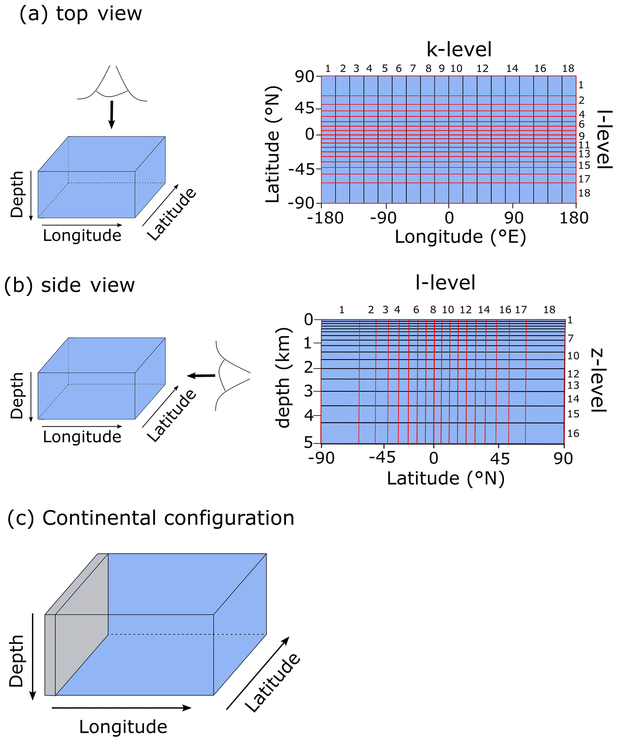
Figure 2Schematic depiction of the cGENIE grid used for our simulations. The grid is , uniform in longitude, and uniform in the sine of latitude. The layer thickness in the vertical grid increases from 80.8 m at the surface to 765 m at the deepest layer. (a) Top view of the cGENIE grid with an indication of the layer numbers. (b) Side view of the cGENIE grid with an indication of the layer numbers. (c) Schematic picture of the continental configuration. “Ridge world” has one continent which runs from pole to pole and extends from 0 to 20∘ E (i.e. the width of a longitudinal grid cell). The ocean is 5000 m deep everywhere.
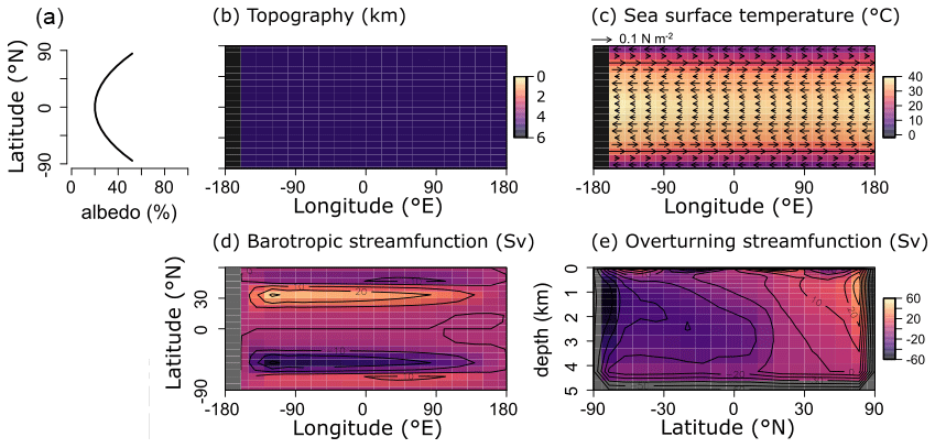
Figure 3(a) Albedo, (b) topography, (c) sea surface temperature and wind stress, and (d, e) ocean circulation patterns for all model runs. (d) Barotropic streamfunction. (e) Overturning streamfunction. Positive values indicate clockwise circulation.
2.2 The biological carbon pump
In this paper, we adapt a representation of biological export from the surface ocean driven by an implicit (i.e. unresolved) biological community with a highly parameterized uptake of nutrients in the photic zone. The description of the basic scheme can be found in Ridgwell et al. (2007), although we use the specific configuration (including iron co-limitation) following Tagliabue et al. (2016). The governing equations are summarized below.
Biological productivity in the euphotic zone (taken to be the surface layer in the ocean model) is controlled by dissolved phosphate () and dissolved iron (Fe, which we will define later) availability, the fractional ice coverage of each grid cell (A), mean ambient light, and temperature. With the exception of the parameterization of the temperature term, the equation for photosynthetic nutrient uptake (M h−1) follows Doney et al. (2006).
Rates of photosynthetic nutrient uptake are scaled to ambient dissolved nutrient concentrations ( and Fe3+) according to an optimal uptake timescale (τbio=1521.6 h; Meyer et al., 2016) and converting [Fe] to the equivalent dissolved phosphate concentration via the Fe:P Redfield ratio (). The various limitation terms (all unitless) are
where shortwave irradiance I is averaged over the entire mixed layer and is assumed to decay exponentially from the sea surface with a length scale of 20 m, as per Doney et al. (2006). The κ terms in each equation represent half-saturation constants for each limiting component (κI=40 W m−2, =0.1 µM, nM) and are as used in Tagliabue et al. (2016). The influence of temperature on biological export is parameterized as
where kT0 (0.59) is a scaling constant, keT (15.8 ∘C) the e-folding temperature, and T is the in situ temperature (∘C). The scaling constants give rise to an approximately factor of 2 change per temperature change of 10 ∘C (Reinhard et al., 2020a).
A proportion (ν=0.66) of taken up by biota is partitioned into dissolved organic phosphorus (DOP), while the remainder – as particulate organic phosphorus (POP) – is exported vertically out of the surface ocean. The value of ν has been assigned following the assumptions of the OCMIP-2 protocol (Najjar and Orr, 1999) (there is also an option for enacting temperature-dependent partitioning – and remineralization – of DOP, which presents an alternative to the fixed DOP–POP partitioning used here; Crichton et al., 2021). Because the biological configuration used here does not resolve explicit standing plankton biomass, the export flux of POP () is always equal to the rate of uptake:
where ρ is the density of seawater (kg m−3) and he the thickness of the euphotic zone (80.84 m). The particulate organic carbon (POC) export flux () is calculated using a fixed Redfield ratio as
After export from the surface grid cells, POC is remineralized instantaneously throughout the water column following a Martin-type curve (Martin et al., 1987), with a specified decay constant b (0.7) (Fig. 4a):
The b value of 0.7 is slightly higher than the global average of 0.6 estimated based on modern observations by Henson et al. (2011), but it leads to a better reconstruction of the distribution of CaCO3 in deep-sea sediments (Jamie Wilson, personal communication).
The motivation behind this paper is to provide a tool that can aid understanding of the key interactions between the biological carbon pump, the oxygenation of the atmosphere and ocean, and the marine biogeochemical cycles of iron (Fe) and sulfur (S). In taking the first step towards this end, we construct a parsimonious model of ocean biogeochemical cycling based on a simplified speciation scheme for both Fe and S, and we only consider a relatively limited number of potential redox states. In this section we briefly describe the general conceptual cycle of Fe and S, as illustrated in Fig. 4b, and in the following subsections discuss the assumptions, reaction equations, and parameters for each cycle. The model equations that describe the biogeochemical reactions (summarized in Table 1) are given in Table 2, and the kinetic constants, their units, and default values can be found in Table 3.

Figure 4(a) Example of the Martin curve for vertical organic matter fluxes in the ocean. (b) Conceptual description of the iron–sulfur cycle implemented in the model. For simplicity, only FeOOH (oxidized iron) and Fe2+ (reduced iron) are depicted, but the model includes different iron species in both the oxic and anoxic states. Interaction between the methane cycle and sulfur cycle is omitted for clarity. See text for details.
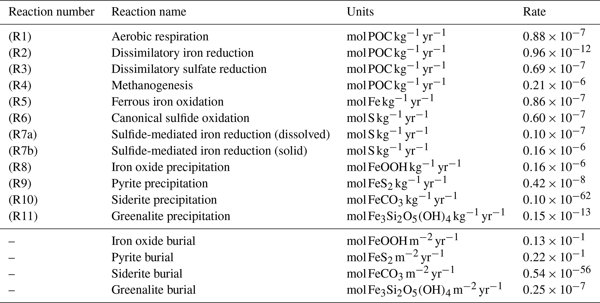
Table 1List of biogeochemical reactions included in the reduced Fe–S scheme within the cGENIE model. A distinction is made between mineralization (“primary redox reactions”), re-oxidation of reduced products (“secondary redox reactions”), and precipitation reactions. The associated kinetic expressions are listed in Table 2. Note that we do not include any details for reactions involving the methane cycle here, though they are included in the simulations described here. For more information about the parameterization and reactions of the methane cycle in cGENIE, we refer the reader to Reinhard et al. (2020a).
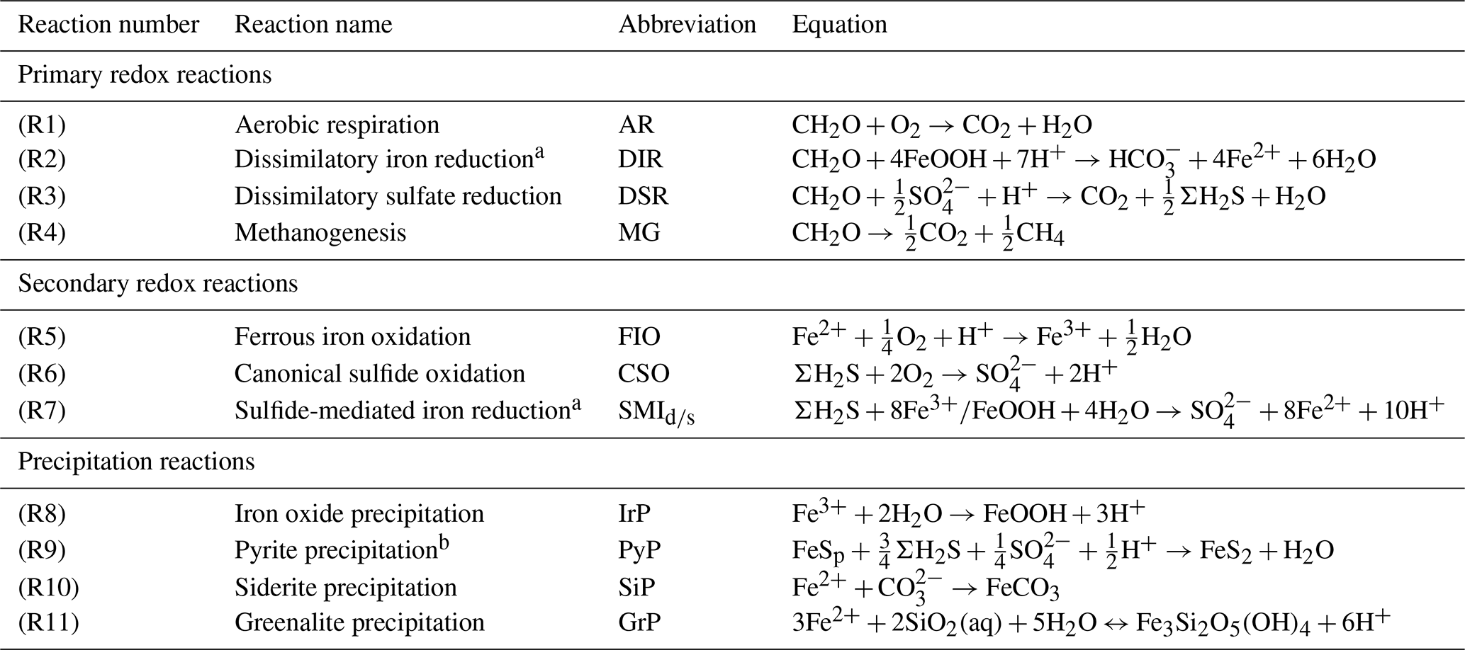
a DIR can only occur with solid-phase FeOOH, whereas SMI can occur with dissolved Fe3+ and solid-phase FeOOH. See text for more details. b The calculation of FeSp occurs implicitly from the concentrations of Fe2+ and ΣH2S as well as the solubility of FeSaq; see Sect. 3.1.3 for more details.
Redox cycling in the ocean (and sediments) is driven by the mineralization of POC, which is produced in the photic zone by photosynthesis and subsequently sinks through the water column (Ridgwell et al., 2007). A Martin-type decay curve of organic matter flux with depth is prescribed in the model such that regardless of the relative availability of different electron acceptors, the fraction of organic matter that will be degraded (relative to the amount of organic matter produced in the photic zone) is depth-dependent. We avoid the alternative here – a fully kinetic set of equations wherein each electron acceptor is associated with a different rate of degradation – partly because of the additional set of poorly constrained (kinetic rate constant) parameters that would be required and partly because implementing such a scheme effectively requires knowledge about the composition of settling organic matter and how its relative reactivity changes with time (Ridgwell, 2011; LaRowe and Van Cappellen, 2011). Thus, the mineralization rate is dependent on the magnitude of the POC flux, which follows a Martin-type decay (Fig. 4a) that determines the mineralization rate (Rmin) at each depth layer in the water column, and thus Rmin (M h−1) at depth z is calculated as
where Δz is the thickness of the grid cell at depth z (in metres). Note that mineralization of particulate organic matter only occurs below the surface layers; z>1 in Fig. 2. The mineralization of POC is coupled to the reduction of a terminal electron acceptor (TEA). These TEAs are used according to decreasing energy yield (Froelich et al., 1979), and relative consumption rates are scaled with TEA concentration and the local abundance of inhibitory substances (i.e. a more energy-yielding TEA). Our mineralization scheme includes aerobic respiration (AR, R1 in Table 1), dissimilatory iron reduction (DIR, R2 in Table 1), dissimilatory sulfate reduction (DSR, R3 in Table 1), and methanogenesis (MG, R4 in Table 1). Of these, AR and DSR existed in the original cGENIE biogeochemical framework (Ridgwell et al., 2007), while methanogenesis has been more recently added (Reinhard et al., 2020a). In the current paper, we ignore nitrate reduction (Monteiro et al., 2012).
The rate of TEA consumption is represented by a Michaelis–Menten type of relationship with respect to TEA concentration that allows for a non-linear closure of the system.
Here, K0 represents the half-saturation constants for the four primary redox reactions and Ki represents the inhibition constants that act on the less energetic redox reaction (Table 3). The consequence of this scheme is that in the oxic zone of the water column, aerobic respiration is responsible for nearly all of the POC mineralization. When oxygen starts to become depleted, DIR and subsequently DSR become the dominant mineralization pathways. When both iron oxides and sulfate are exhausted, MG represents the final mineralization pathway. While the occurrence and parameterization of DSR and MG in the water column are relatively straightforward, the possibility of DIR in the water column is more complex and is discussed in more detail in Sect. 3.1.2.
Table 2List of kinetic rate expressions for the reactions included in the cGENIE model. All expressions are based on standard kinetic formulations in biogeochemical models. The values of the kinetic constants are listed in Table 3.
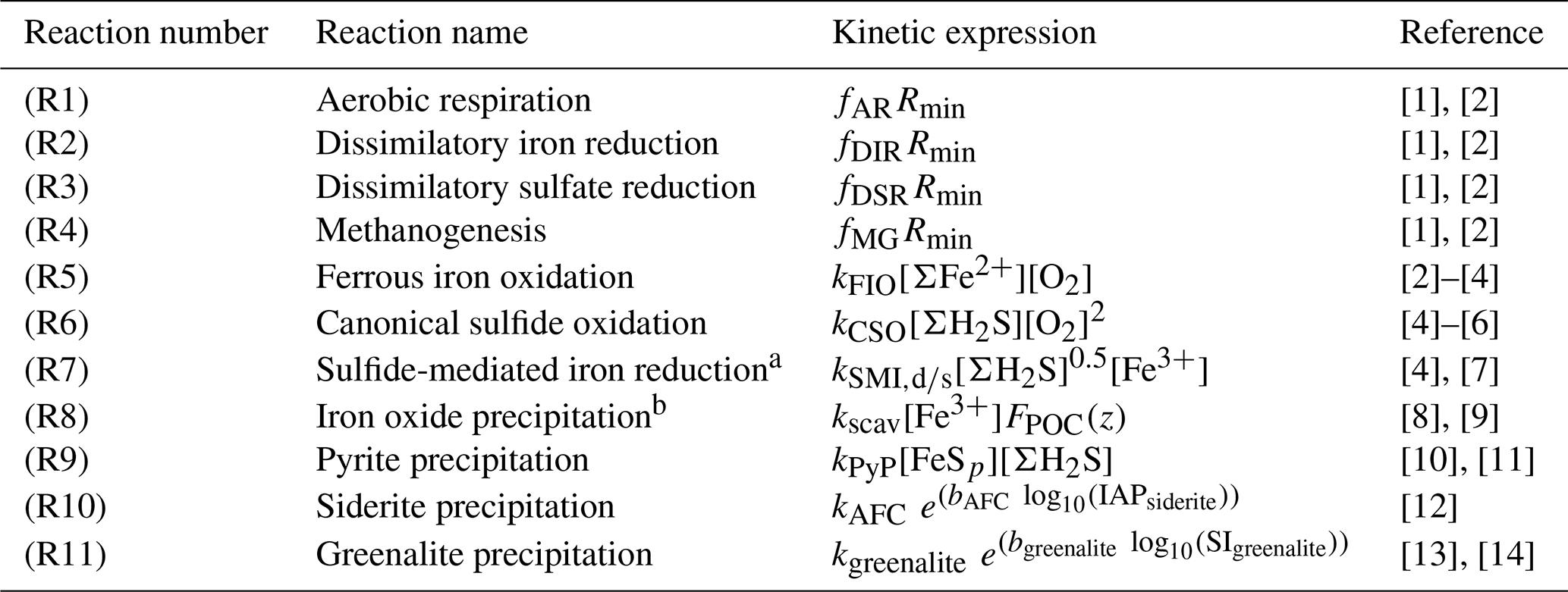
a Two different kinetic constants are used for the reactions between Fe3+ and sulfide (kSMI,d) and between FeOOH and sulfide (kSMI,s); see text for details. b The formation of iron oxide minerals is parameterized according to Parekh et al. (2004) and is explained in more detail in Sect. 3.1.1. References: [1] Soetaert et al. (1996), [2] van de Velde and Meysman (2016), [3] Millero et al. (1987a), [4] Dale et al. (2015), [5] Ridgwell et al. (2007), [6] Zhang and Millero (1993), [7] Poulton et al. (2004), [8] Parekh et al. (2004), [9] Tagliabue et al. (2016), [10] Rickard (1997), [11] Rickard (2006), [12] Jiang and Tosca (2019), [13] Tosca et al. (2015), [14] Rasmussen et al. (2015)
As a consequence of organic matter remineralization in the model, DIR produces ferrous iron (Fe2+), which is re-oxidized when it comes into contact with oxygen (e.g. via upwelling of the reduced compound or downwelling of oxygen) via ferrous iron oxidation (FIO, R5 in Table 1) (Millero et al., 1987a). Similarly, any reduced sulfide (because we do not consider sulfide speciation explicitly, reduced sulfide is defined as ) that comes into contact with oxygen is re-oxidized via canonical sulfur oxidation (CSO, R6 in Table 1) (Millero et al., 1987b). Additionally, H2S is oxidized by reaction with oxidized iron via sulfide-mediated iron reduction (SMI, R7 in Table 1) (Fig. 4b; Canfield et al., 1992; Poulton et al., 2004; Mikucki et al., 2009). The oxidized form of iron, ferric iron (Fe3+), will precipitate out as iron oxide (FeOOH) minerals (IrP, R8 in Table 1).
When Fe2+ and H2S are simultaneously present in the water column they form dissolved FeS (FeSaq). Once FeSaq surpasses a solubility threshold of ∼2 µM (Rickard, 2006), particulate FeSp can form, which further reacts with H2S to form the mineral pyrite (FeS2) via pyrite precipitation (PyP, R9 in Table 1) (Rickard, 1997). Alternatively, when Fe2+ accumulates past its saturation state with bicarbonate, siderite (FeCO3) forms via siderite precipitation (SiP, R10 in Table 1) (Jimenez-Lopez et al., 2004; Jiang and Tosca, 2019). Finally, greenalite (Fe3Si2O5(OH)4) precipitates when Fe2+ and dissolved silica (SiO2) are saturated with respect to greenalite precipitation (GrP, R11 in Table 1) (Tosca et al., 2015; Rasmussen et al., 2015). Pyrite, siderite, and greenalite are subsequently buried in the sediment, together with any solid FeOOH that has not reacted (the half-life of iron oxides in euxinic waters is of the order of tens to hundreds of days, which is comparable to the residence time of a particle in the ocean; Poulton et al., 2004) (Fig. 4b). These four solid-iron phases are the main burial phases for reactive iron and form the basis of the Fe-speciation proxy used to reconstruct local redox conditions in past oceans (Poulton and Canfield, 2011). It should be noted, however, that some of these phases can undergo transformations to other phases in the sediment after deposition (such as greenalite to magnetite). In our current model set-up, no sedimentary processes are included, but future developments will address the sedimentary part of the Fe and S cycle.
Many of the iron and sulfur reactions can go to completion much faster than the biogeochemical time step ( year in the example conceptual configuration) under typical modern or paleo-geochemical conditions. This can create negative tracer concentrations because transport by ocean circulation acts concurrently on the tracer field in our numerical scheme. We hence place a limit on reactant consumption for any reaction in which a reactant would be completely consumed in a single time step. Specifically, we prescribe a maximum timescale for all geochemical reactions, for which in this paper we chose a value of 45 d.
3.1 The iron cycle
The cGENIE model already included the representation of a simplified iron cycle designed to account for iron limitation of biological productivity at the ocean surface (Tagliabue et al., 2016). However, because its initial use was to model the present-day oceanic iron cycle, it does not contain an anoxic iron cycle (as 95 % of today's ocean volume is oxic; Diaz and Rosenberg, 2008) or any coupling between the iron and sulfur cycles (e.g. via the precipitation of FeS2). The absence of an anoxic iron cycle limits the suitability of cGENIE for simulating low-oxygen worlds in which the ocean interior is pervasively anoxic and iron and sulfur cycling would have dominated ocean biogeochemistry (Poulton and Canfield, 2011; Raiswell and Canfield, 2012). In addition to summarizing the existing oxic cycle, we expand the model to include key processes operating in anoxic environments.
3.1.1 The oxic iron cycle
In oxygenated waters, iron is predominately present in its oxidized form (Fe3+). The oxic iron cycle in cGENIE follows Parekh et al. (2004) and has been recently updated with a revised set of parameters calibrated based on the present-day iron cycle (Tagliabue et al., 2016). Briefly, in the previous scheme total dissolved Fe3+ consists of free and ligand-bound , with only the “free” fraction being subject to scavenging on particulate organic carbon (POC) particles (whereas both free and ligand-bound dissolved iron phases are assumed to be bioavailable and fuel primary productivity; see Sect. 2.2). When scavenged on POC, FeOOH sinks as a “marine snow” particle through the water column. This scavenging mechanism is commonly used in reactive-transport models of ferruginous lakes or the modern ocean (see e.g. Taillefert and Gaillard, 2002; Tagliabue et al., 2016). Marine snow formation is what likely happens today, whereby relatively high production of organic matter drives the transport of chemically heterogeneous aggregates (containing iron oxides or barite; Dehairs et al., 1990; Balzano et al., 2009). The scavenging rate of iron is a function of the concentration of together with the magnitude of the POC flux from the grid cell, i.e.
where kscav ( mol−1 m2) is a scavenging constant calibrated to the modern-day distribution of Fe (Tagliabue et al., 2016). We assume that the complexation reaction is always in equilibrium, which allows for the calculation of the amount of at each time step by the conservation equations.
Here, is the stability constant of the complex (1.0×10¹¹ M−1; Table 3), Lfree is ligand unassociated with Fe3+, and Ltotal is the total amount of ligand.
Oxidized iron is highly insoluble in seawater and will rapidly form particulate oxides (FeOOH), driving down equilibrium dissolved Fe3+ abundance to picomolar values without stabilization by ligands (Liu and Millero, 2002). Thus, will form colloidal or nanoparticulate iron oxides – FeOOH – which can then adsorb on other particles or aggregate to bigger particles and sink through the water column (Raiswell and Canfield, 2012). In cGENIE, the pool of can be thought of as a mix of purely dissolved Fe3+ and a range of colloidal and nanoparticulate Fe3+ phases that do not settle efficiently through the water column. The pool can then further react or scavenge onto particles that allow it to more effectively settle through the water column.
In our new formulation of the Fe cycle in cGENIE, (that is not stabilized by ligands) is still the phase that is scavenged by settling POC (using a fixed scavenging rate; Eq. 11), but it is explicitly assumed to be in the form of FeOOH and can be used for DIR when oxygen becomes depleted (see Sect. 3.1.2). We also provide the option in the model for to precipitate as a pure FeOOH phase, without being associated with POC. In this case, dissimilatory iron reduction does not occur in the water column since both POC and FeOOH are not associated within the same particle. This situation would be more appropriate in the case of high amounts of iron oxidation and lower production of organic matter (which was potentially the case in the Archean; Thompson et al., 2019). This configuration is by default implemented using a numerical “cut-off”, at which all that passes the solubility threshold of 0.5 nM (Liu and Millero, 2002) is considered particulate and sinks through the water column.
To close the oceanic iron cycle, we have introduced a new dissolved iron species, Fe2+. Any reduced Fe2+ that is mixed into the oxic zone is being rapidly oxidize to Fe3+ via ferrous iron oxidation (FIO):
where the rate equation can be expressed as
and where kFIO is a reaction rate constant ( ) (Table 2; Millero et al., 1987a). In the calculation of the nutrient limitation of biological production at the surface, Fe2+ is also assumed to be bioavailable, meaning that iron limitation is calculated from the total dissolved iron pool, equal to .
In summary, we have extended the basic representation of Parekh et al. (2004), which considered only a generic free “dissolved” iron (that could be scavenged) and a ligand-bound iron phase, to now distinguish between the oxidation states of iron (and the tracers Fe2+ and Fe3+), with Fe3+ being split (as previously) into a free (and scavengeable) and ligand-bound phase.
3.1.2 The anoxic iron cycle
In an anoxic water column, oxidized forms of iron can be reduced to Fe2+ either via dissimilatory iron reduction or via sulfur-mediated iron reduction. We describe the two processes individually as follows.
Dissimilatory iron reduction in the water column
The majority of oxidized iron exists in particulate form due to the low solubility of Fe3+, which poses a challenge for micro-organisms performing dissimilatory iron reduction in the water column. Iron reducers need physical contact with the iron mineral to reduce iron (Gorby, 2006), which is difficult when both organic matter and FeOOH are in particulate form and are dispersed separately throughout the aqueous medium. Even in a sediment column in which all particles are packed closely together, DIR generally requires sediment homogenization by burrowing fauna to become volumetrically important (Thamdrup, 2000; van de Velde and Meysman, 2016). Indeed, in a sulfate-rich, ancient marine brine, Fe3+ was found to be the terminal electron acceptor, but sulfur ultimately acted as a redox shuttle between organic matter and iron oxides (Mikucki et al., 2009). Studies of anoxic Lake Pavin suggest that most of the iron reduction occurs in the sediment rather than the water column (Michard et al., 1994; Cosmidis et al., 2014), although the same studies indicated that manganese oxide reduction (which has a very similar mechanism and inhibition concentration as DIR; Lovley, 1991; Thamdrup, 2000) does occur in the water column. However, there is direct evidence for iron reduction occurring coupled to organic matter mineralization in the water column in a range of other anoxic lakes, such as Lake Sammamish (Washington, USA; Balistrieri et al., 1992), Lake Cadagno (Switzerland; Berg et al., 2016), Lake Matano (Indonesia; Crowe et al., 2008), and Paul Lake (Michigan, USA; Taillefert and Gaillard, 2002). These studies suggested that DIR was coupled to either the oxidation of dissolved organic matter (Crowe et al., 2008) or reduction of iron in aggregates with organic matter. The latter has been experimentally shown to occur (Balzano et al., 2009). We consider this to be strong evidence that DIR can be coupled to POC oxidation in a water column, especially in the ocean where the residence time of particles is considerably longer than in a much shallower lake environment.
To model DIR in the water column, we use the mathematical expression of DIR in marine sediments, where FeOOH is a common electron acceptor for organic matter mineralization (Thamdrup, 2000). Dissimilatory iron reduction has an overall reaction stoichiometry of
where it is implicitly assumed that every iron oxide particle consists solely of Fe3+ rather than a mixture of redox states, as is sometimes encountered at the interface of ferruginous lakes (Zegeye et al., 2012). This assumption greatly simplifies the reaction scheme and parameter set. Dissimilatory iron reduction generally becomes limited when concentrations of FeOOH drop below M (Van Cappellen and Wang, 1996; Thamdrup, 2000). This limitation is expressed as in Eq. (10) and follows the conventional limitation–inhibition scheme (Soetaert et al., 1996), whereby the parameter K0,FeOOH expresses the concentration at which DIR occurs at half of its maximum rate (the maximum rate is set by Rmin; see Eq. 10 and Table 2). In marine sediments, DIR generally occurs before sulfate reduction since it is a more energy-yielding electron acceptor (Thamdrup, 2000), although the wide range of reactivities for different iron oxide minerals often leads to an overlap of DIR and DSR zones (Postma and Jakobsen, 1996). This limitation is expressed as in Eq. (10), where Ki,FeOOH expresses the concentration above which FeOOH inhibits other mineralization pathways (DSR and MG). In early diagenetic models, this concentration is generally assumed to be identical to the limitation parameter K0,FeOOH (Van Cappellen and Wang, 1996; Soetaert et al., 1996; van de Velde and Meysman, 2016). As a baseline value, we assume that K0,FeOOH and Ki,FeOOH both equal 10−3 M (comparable to the inhibition concentration in marine sediments), but as explained above, these parameter values are subject to a high degree of uncertainty. Therefore, we include parameters K0,FeOOH and Ki,FeOOH in our model sensitivity testing (Sect. 4.3).
Sulfur-mediated iron reduction
Oxidized iron in the ocean can also be reduced via sulfur-mediated iron reduction (SMI), which follows the stoichiometry (Poulton et al., 2004)
We are not explicitly modelling elemental sulfur (S0) but assume that it becomes quantitatively disproportionated into H2S and (Finster et al., 1998),
which then leads to the overall stoichiometry
Note that [Fe3+] in Eq. (19) can represent dissolved Fe3+ or solid FeOOH. The assumption of quantitative disproportionation implies that pyrite precipitation is not closely coupled to the reaction between ΣH2S and Fe3+ but only occurs via precipitation of FeSp with ΣH2S (see Sect. 3.1.3). Laboratory experiments have shown that this assumption is valid for aquatic systems in which Fe3+ is not in excess with respect to ΣH2S (Wan et al., 2017), which is the case for most modern marine systems. We contend that this is also a valid assumption for water-column chemistry for most of Earth's history, as rapid settling of oxidized particulate FeOOH through the water column would prevent high concentrations of Fe3+ (in the water column). To achieve an excess of Fe3+ over ΣH2S, the ΣH2S concentrations would have to be even lower, leading to very negligible rates of iron reduction. However, this reaction pathway would likely become important in the sediment of a low-sulfate ocean (i.e. periods of Archean time).
The kinetic rate for Reaction (18) can then be expressed as (Poulton et al., 2004)
We assume that the dissolved form is highly reactive with sulfide (a reaction time of ∼5 min, which is comparable to the reactivity of freshly precipitated hydrous ferric oxide) and has a reaction rate constant of (Poulton et al., 2004). The solid form of FeOOH can represent a number of different oxidized iron minerals which are reactive towards sulfide on timescales ranging from hours to hundreds of days (Poulton et al., 2004). For our baseline simulations, we assume that all FeOOH precipitates as lepidocrocite, which has a reactivity constant of (Poulton et al., 2004). Lepidocrocite is less crystalline than the other (non-hydrous) iron oxides and precipitates when the rate of Fe3+ supply is low relative to the rate of precipitation, as is generally the case in natural systems (Crosby et al., 1983). We discuss the model sensitivity to choices of kSMI,s in Sect. 4.3. The reduction of Fe3+ produces Fe2+, which can either be re-oxidized when it comes in contact with O2 (see Sect. 3.1.1) or can form reduced minerals.
Both reduction and oxidation reactions of dissolved iron, even with dissolved O2 and ΣH2S in nanomolar (nM) concentrations, can proceed very rapidly and are hence subject to the geochemical reaction rate limitation described earlier. Furthermore, because these two reactions form a coupled oxidation–reduction pair, we limit the fastest reaction according to a 45 d timescale but limit the slower one in proportion to their relative unmodified reactions rates. We thereby simulate an equilibrium partitioning between Fe2+ and Fe3+ according to ambient dissolved oxygen and sulfide concentrations.
3.1.3 Reduced iron mineral formation
Reduced Fe2+ can form complexes with a number of inorganic ligands that are common in seawater, including Cl−, , and bicarbonate (Millero et al., 1995). Under anoxic conditions, however, the most important inorganic ligand is free sulfide (Rickard, 2006), which is produced by sulfate reduction. Together, dissolved and the aqueous iron-sulfide complex (FeSaq) make up ∼100 % of the total dissolved iron pool in sulfidic–anoxic seawater (Fig. 5a). The thermodynamic equilibrium can be calculated as
which was obtained from the visualMINTEQ database (Gustafsson, 2019) and is based on stability constants calculated by Luther et al. (1996).
Since dissolved and the FeSaq complex are the dominant dissolved forms of reduced ferrous iron in natural waters (in anoxic seawater devoid of sulfide, dissolved still represents ∼80 % of the dissolved Fe2+ pool; Fig. 5b), we choose to only consider those two species. We do not explicitly model the FeSaq complex but calculate the thermodynamic equilibrium before each reaction proceeds, implicitly assuming that it is reached much faster than any of the kinetic reactions in our reaction set (as is commonly done for the complexation of Fe3+; see Sect. 3.1.1). This is important, since FeSaq forms particulate FeSp, which is the precursor of pyrite (FeS2) (Rickard, 1997, 2006). Furthermore, siderite or greenalite can only precipitate from (Tucker, 2001; Tosca et al., 2015), and their precipitation rates are consequently dependent on the dissolved concentration.

Figure 5Relative importance of different dissolved Fe complexes, obtained by visualMINTEQ (Gustafsson, 2019). Concentrations of other constituents are chosen to represent average seawater, with the dissolved organic carbon (DOC) concentration from Sharp et al. (1995).
Before each precipitation reaction, we calculate the concentration of FeSaq, , and H2Sfree using Eq. (20). We then compare the FeSaq concentration to the solubility threshold (10−5.7 M; Rickard, 2006). If FeSaq surpasses the solubility value, the fraction above the solubility concentration precipitates instantaneously as particulate iron monosulfide (FeSp) (Suits and Wilkin, 1998). Note that here we consider FeSp solubility to be independent of pH, which should be valid for seawater pH above 7 (Rickard, 2006). Pyrite can then form locally via reaction between FeSp and free ΣH2S, with the production of free hydrogen gas (as S2− in ΣH2S and FeSp has to be oxidized to S1− in FeS2; Rickard, 1997):
Since hydrogen gas is highly reactive, it is almost instantaneously oxidized with the reduction of an electron acceptor like O2, , or CO2. Given that pyrite precipitates under sulfidic conditions, oxygen is absent, and sulfate is the most likely electron acceptor.
To preserve the redox balance while avoiding the need to model an additional state variable (H2), we can combine Reactions (21) and (22) to
By using Eq. (23) we implicitly assume that the hydrogen gas produced during pyrite precipitation immediately reacts with . Since pyrite formation is not an equilibrium reaction (pyrite minerals are stable in seawater), the reaction of pyrite is described as a kinetic reaction with a second-order dependency on [FeSp] and [ΣH2S], with (Rickard, 1997). The rate equation for FeS2 precipitation can then be written as
Any Fe2+ that is not complexed with sulfide () can form siderite (FeCO3), an iron–carbonate mineral (Tucker, 2001).
Recent experiments by Jiang and Tosca (2019) have shown that the precipitation of iron–carbonate phases is controlled by the formation of amorphous Fe carbonate (AFC), which has the stoichiometric formula . Since the thermodynamic data required to calculate the mineral solubility product of AFC are currently lacking, Jiang and Tosca (2019) have determined the rate of AFC precipitation based on the ion activity product (IAP):
where γ represents the activity coefficient of a given ion in seawater (Table 3). The rate-limiting step in the precipitation reaction is the spontaneous nucleation of AFC, and hence the empirically derived rate of AFC precipitation follows an exponential function that describes the nucleation rate from water (Steefel and Van Cappellen, 1990; Jiang and Tosca, 2019):
where kAFC is M h−1 and bAFC equals 9.042 (Table 3).
Another reduced iron mineral potentially important for anoxic, Fe-rich environments is the iron–silicate mineral greenalite (Fe3Si2O5(OH)4) (Tosca et al., 2015).
The precipitation rate of greenalite is dependent on its degree of supersaturation (i.e. its saturation index), which can be calculated based on its IAP:
where γ represents the activity coefficient of an ion in seawater (Table 3) and its solubility product (Rasmussen et al., 2015):
where equals 3.98×1027 M−1 (Tosca et al., 2015). The rate equation follows an exponential function that describes the nucleation rate from water (as in siderite, see above; Rasmussen et al., 2015; Jiang and Tosca, 2019):
where kgreenalite is M h−1 and bgreenalite equals 1.856 (Table 3).
3.2 The sulfur cycle
The oxidized form of dissolved sulfur in the ocean is sulfate (). Under anaerobic conditions, sulfate is used as a terminal electron acceptor during organic matter remineralization:
The produced sulfide can then be re-oxidized when it comes into contact with oxygen via canonical sulfide oxidation (CSO).
The rate of CSO in cGENIE is dependent on the concentration of the electron donor (ΣH2S) and acceptor (O2) as well as a second-order rate constant (Zhang and Millero, 1993):
Alternatively, ΣH2S can be re-oxidized with Fe3+ (either Fe3+ or solid FeOOH) during sulfide-mediated iron reduction (as described in Reaction 18).
In cGENIE, the eventual sink for sulfur is the precipitation of pyrite (Reaction 21) (ignoring sulfide reacting with organic matter – see Hülse et al., 2019). We do not currently include precipitation of gypsum (CaSO4) in our model description (Fig. 4b). Gypsum is an evaporite mineral that precipitates during regional and episodic events of supersaturation and was likely a less important sulfur sink on a globally integrated basis during Precambrian time or during any other period in which ocean [] was relatively low (Grotzinger and Kasting, 1993; Crowe et al., 2014; Fakhraee et al., 2019). Indeed, there is still some debate as to the time-integrated impact of sulfate evaporites on the steady-state global sulfur cycle even during more recent periods of Earth's history (Halevy et al., 2012; Canfield, 2013). However, due to its episodic nature, gypsum could play an important role as a sulfate source during transient events (for example during events of enhanced weathering of a gypsum-rich source; Shields et al., 2019). Planned future developments to cGENIE will incorporate an explicit gypsum cycle, which would allow us to use the cGENIE.muffin model to investigate transient events of enhanced sulfate delivery to the ocean (see e.g. Shields et al., 2019).
Table 3List of kinetic constants for the reactions included in the cGENIE model. Note that the units are not identical to the units used in the user configuration files for the cGENIE model. A table with the parameter units converted to cGEnIE units is included in Appendix A.
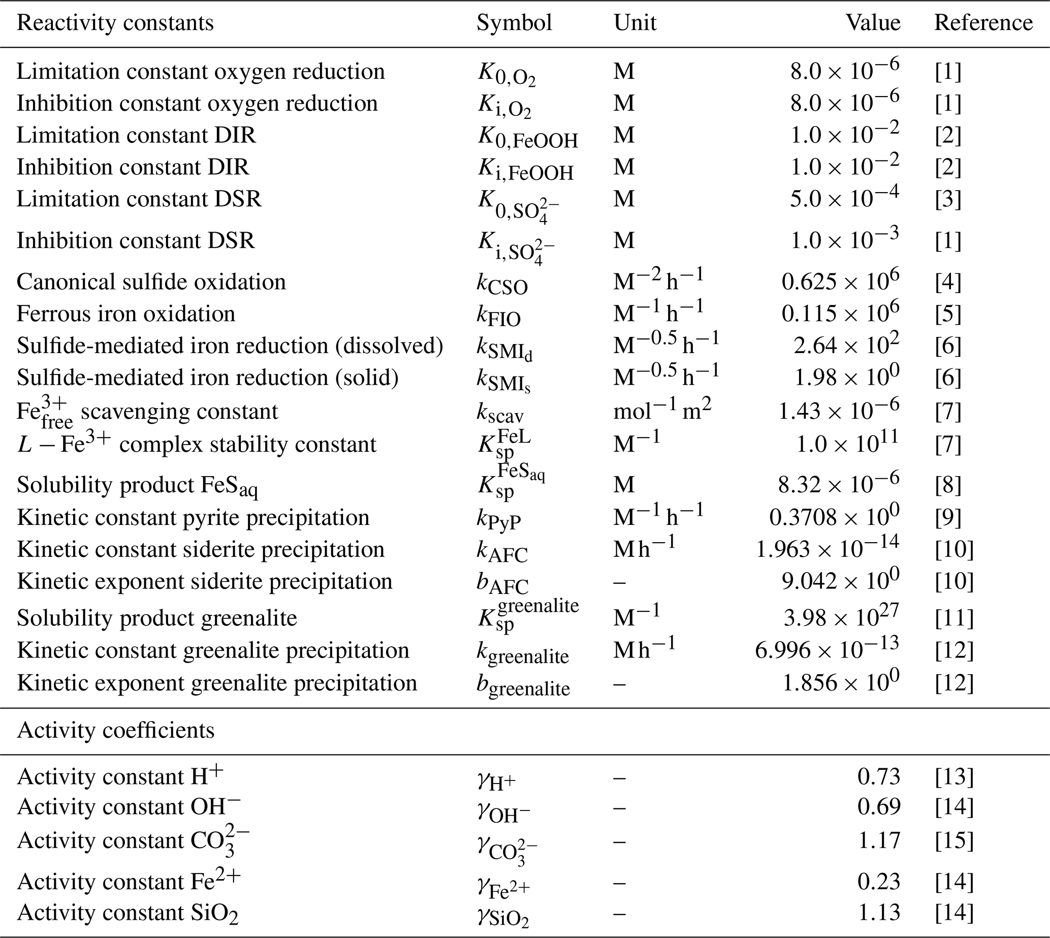
[1] Ridgwell et al. (2007), [2] Thamdrup (2000), [3] Olson et al. (2016), [4] Zhang and Millero (1993), [5] Millero et al. (1987a), [6] Poulton et al. (2004), [7] Ridgwell and Death (2021), [8] Luther et al. (1996), [9] Rickard (1997), [10] Jiang and Tosca (2019), [11] Tosca et al. (2015), [12] Rasmussen et al. (2015), [13] Marion et al. (2011), [14] (following the Davies equation), [15] Johnson (1982).
3.3 Isotope geochemistry
A particularly important application of having a representation of an anoxic Fe–S cycle in cGENIE is exploring ocean redox landscapes during Precambrian time when ocean biogeochemical cycling was dominated by iron and sulfur (Raiswell and Canfield, 2012). As noted above, one way of comparing our model output to available data is the explicit simulation of the burial phases of iron, which allows comparison to the often-used Fe proxy (Poulton and Canfield, 2011). A different and independent constraint potentially exists in the form of Fe or S isotopes (see e.g. Beard et al., 1999; Gomes and Johnston, 2017; van de Velde et al., 2018).
Any chemical element with multiple stable isotopes (Fe, for example, has four stable forms: 54Fe, 56Fe, 57Fe, and 58Fe) can potentially be used to track physicochemical processes that act to partition stable isotopes according to thermodynamic or kinetic principles. For Fe the most abundant isotopes are 54Fe and 56Fe, and deviations in the ratio of Fe-bearing aqueous and mineral phases from that of a reference material can be described using conventional δ notation:
where is the isotope ratio of a standard reference material (IRMM-14). Any geochemical reaction, be it biotic (mediated by micro-organisms) or abiotic, can induce isotopic fractionation between co-occurring Fe- or S-bearing phases.
To model the isotopic signatures of Fe and S, we track the concentrations of the “bulk” pools (Ci) and the isotope-specific pools (56Ci, for example, in the case of Fe). The isotopic signature of an Fe species Ci is then calculated as
Each individual reaction Rk is assigned a fractionation factor (‰; Table 4), which relates to as
Isotope fractionation is then implemented by calculating an isotope-specific reaction rate (for the 56Fe pool) from the bulk reaction rate Rk:
where
In this way, we assign a fractionation factor to each of the reactions considered in our model and are able to track the isotopic signature of each Fe and S species. This allows us to simulate the δ56Fe and δ34S values of dissolved species and solid mineral phases, both of which can potentially be compared to observations from the geological record.
The obvious limitation of assigning a constant fractionation factor to each reaction is that this is incapable of fully capturing natural isotopic variability. For instance, different microbial strains of sulfur reducers (or iron oxidizers) express different fractionation factors, even though the overall reaction remains the same (Gomes and Johnston, 2017; Pellerin et al., 2019). This is reflected in the often broad range of isotopic fractionation factors found in the literature for a given process (Table 4). Other factors influencing microbial fractionation are local environmental conditions, such as electron donor type and availability (Wing and Halevy, 2014; Pellerin et al., 2018) or evolutionary adaptation (Pellerin et al., 2015). Aside from biologically mediated transformations, kinetic effects associated with abiotic aqueous reactions and precipitation of solid phases also affect the fractionation that is eventually recorded in the end product. All these factors can make interpretation of isotope fractionations very complex in natural settings, and it is thus highly unlikely that any particular model simulation will be able to exactly reproduce observed isotope records. Nevertheless, the scheme employed here should be able to discern first-order observations from the geologic record and in some cases could potentially be used to rule out particular endmember hypotheses for ocean chemistry.
Table 4Isotope fractionation factors.
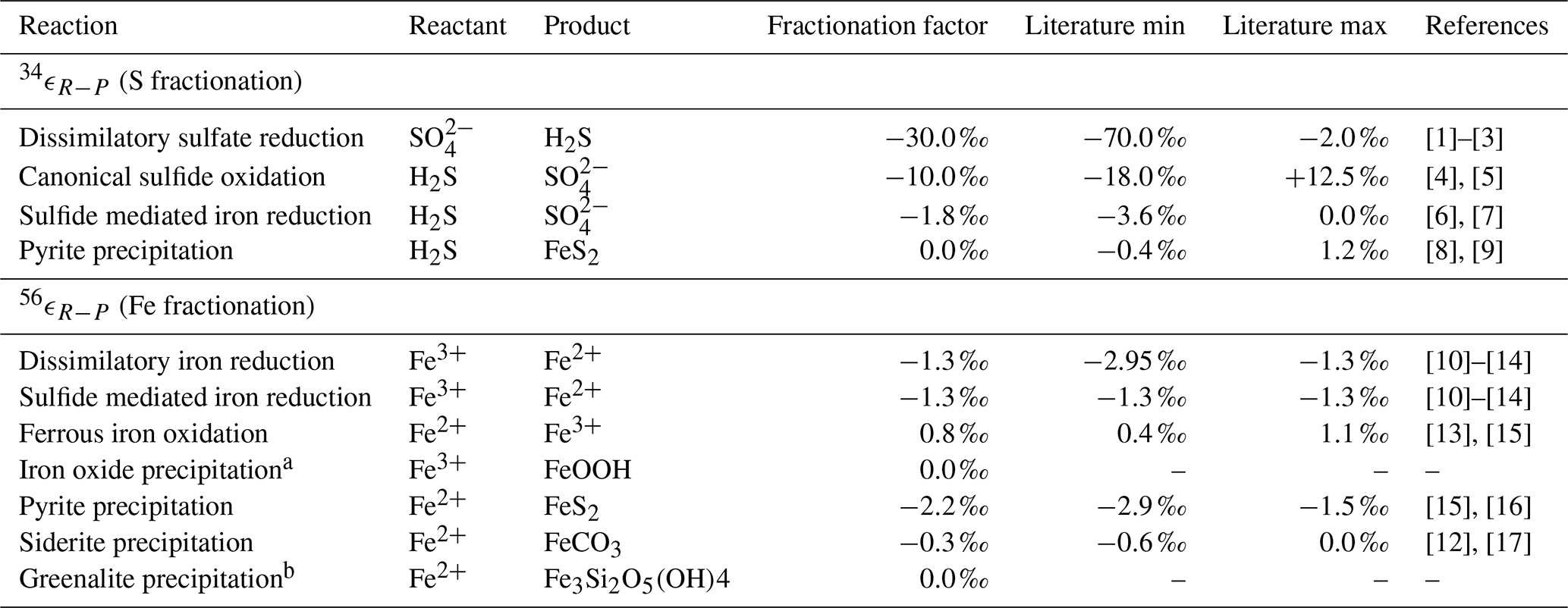
[1] Kaplan and Rittenberg (1964), [2] Detmers et al. (2001), [3] Sim et al. (2011), [4] Gomes and Johnston (2017), [5] Pellerin et al. (2019), [6] Poser et al. (2014), [7] Fry et al. (1988), [8] Bottcher et al. (1998), [9] Price and Shieh (1979), [10] Beard et al. (1999), [11] Beard et al. (2003), [12] Johnson et al. (2004), [13] Bullen et al. (2001), [14] Crosby et al. (2007), [15] Rolison et al. (2018), [16] Guilbaud et al. (2011), [17] Wiesli et al. (2004).
a The isotopic fractionation for iron oxide precipitation is
driven by the oxidation reaction (FIO). b The isotope fraction factor for greenalite precipitation is currently unknown.
We evaluate our model in two ways. We first test whether our extended model code is able to reproduce the Fe cycle of the contemporary oxygenated ocean by comparing it with the previously validated standard (oxic) Fe cycle in cGEnIE (Tagliabue et al., 2016). Secondly, we assess how the model behaves in an ocean which is predominantly anoxic. For contrasting with observations, we are severely limited because the modern ocean is largely well-oxygenated, with only a few oxygen-minimum zones near highly productive margins such as the Indian Ocean and the Peruvian margin (Keeling et al., 2010). However, even in these regions dissolved oxygen concentrations rarely reach zero, and the development of ferruginous or euxinic conditions is essentially absent. Only highly restricted basins such as the Cariaco Basin or the Black Sea and Baltic Sea can develop euxinic conditions, but these conditions arise as a result of local circulation within silled or enclosed basins and are not likely to be representative of an anoxic open-ocean setting. As a result, we lack observations to which we can directly calibrate our model. However, as our model development consisted of the implementation of well-established, mechanistic biogeochemical reactions with relatively well-defined kinetic rates, our model should simulate realistic rates and concentrations without extensive calibration of model parameters. We illustrate this by showing the spatial concentration and isotope features of a hypothetical anoxic ocean (Sect. 4.2) and – where possible – compare our predicted reaction rates to rates obtained from anoxic process analogues for the ancient oceans. Subsequently, we broadly illustrate the sensitivity of the model output to the newly introduced parameters of the iron–sulfur cycling (Sect. 4.3). As discussed below, our model is largely robust across a range of values for key parameters, and it predicts reaction and process rates that are comparable to those obtained experimentally or observed in modern analogue environments.
4.1 The contemporary ocean
We test our new iron scheme in comparison to the results of the oxic-only scheme presented by Tagliabue et al. (2016), which was based on the modern cGENIE configuration of Cao et al. (2009). For clarity, we carry out this test stepwise in two stages in order to separate out the consequences of resolving the different oxidation states of dissolved iron from the various solid-iron reactions.
-
Firstly, we substitute the original three tracers carried in the ocean – free dissolved iron (which we can equate here to ), ligand-bound iron (), and free ligand (Lfree) – for our new tracer scheme of Fe3+ (total = free + ligand-bound), Fe2+, and TDL (total dissolved ligand). Note that in the original scheme only two tracers were actually needed – total dissolved iron (Fe3+) and total dissolved ligand (L) – as the equilibrium between , , and Lfree was re-calculated each time step. Hence, our new tracer scheme is composed of these same two primary tracers (Fe3+, L), plus Fe2+. We then enable the two-way oxidation–reduction reactions: and (Eqs. 13 and 18). We retain the same scavenging scheme as before, with iron scavenged by POM as Fe3+ and not subject to DIR.
-
The step is as per (1), but we now represent scavenged iron as FeOOH and enable DIR (Eq. 15). We also enable SMI of solid FeOOH with ΣH2S (Eq. 18) and pyrite precipitation (Eq. 23). Note that the biogeochemical scheme used in Tagliabue et al. (2016) already included sulfate reduction and sulfide oxidation (DSR and CSO; Eqs. 32 and 33).
We find only minor differences between the old cGEnIE Fe cycling scheme (which only includes an oxic Fe cycle – see above) and the step (1) configuration of our new scheme (Fig. 6). Because the old scheme did not include reduced Fe2+, we compare total dissolved Fe (TDFe), which is the sum of all dissolved Fe phases (i.e. [TDFe] = [Fe3+] + [Fe2+]). Adding Fe2+ as a tracer, which is released during POC oxidation under anoxic conditions, leads to a slight increase in [TDFe] in oxygen-minimum zones (OMZs) (Fig. 6b) because in our new scheme Fe2+ is assumed not to be subject to scavenging. Hence, reducing Fe3+ to Fe2+ reduces iron loss due to scavenging and enhanced TDFe in OMZs. Consequently, there is a slightly enhanced supply of Fe to the surface waters via upwelling, leading to marginally higher surface [TDFe] (∼ 0.02 nM), in particular above the Peruvian OMZ (Fig. 6e). In step 2, by including a full Fe redox cycle (i.e. the reduction of FeOOH coupled to POC oxidation or sulfide oxidation) this effect is slightly intensified, with DIR and SMI leading to an additional reduction of Fe3+ (as FeOOH) and release of Fe2+ (which again escapes scavenging). (Fig. 6c, f).
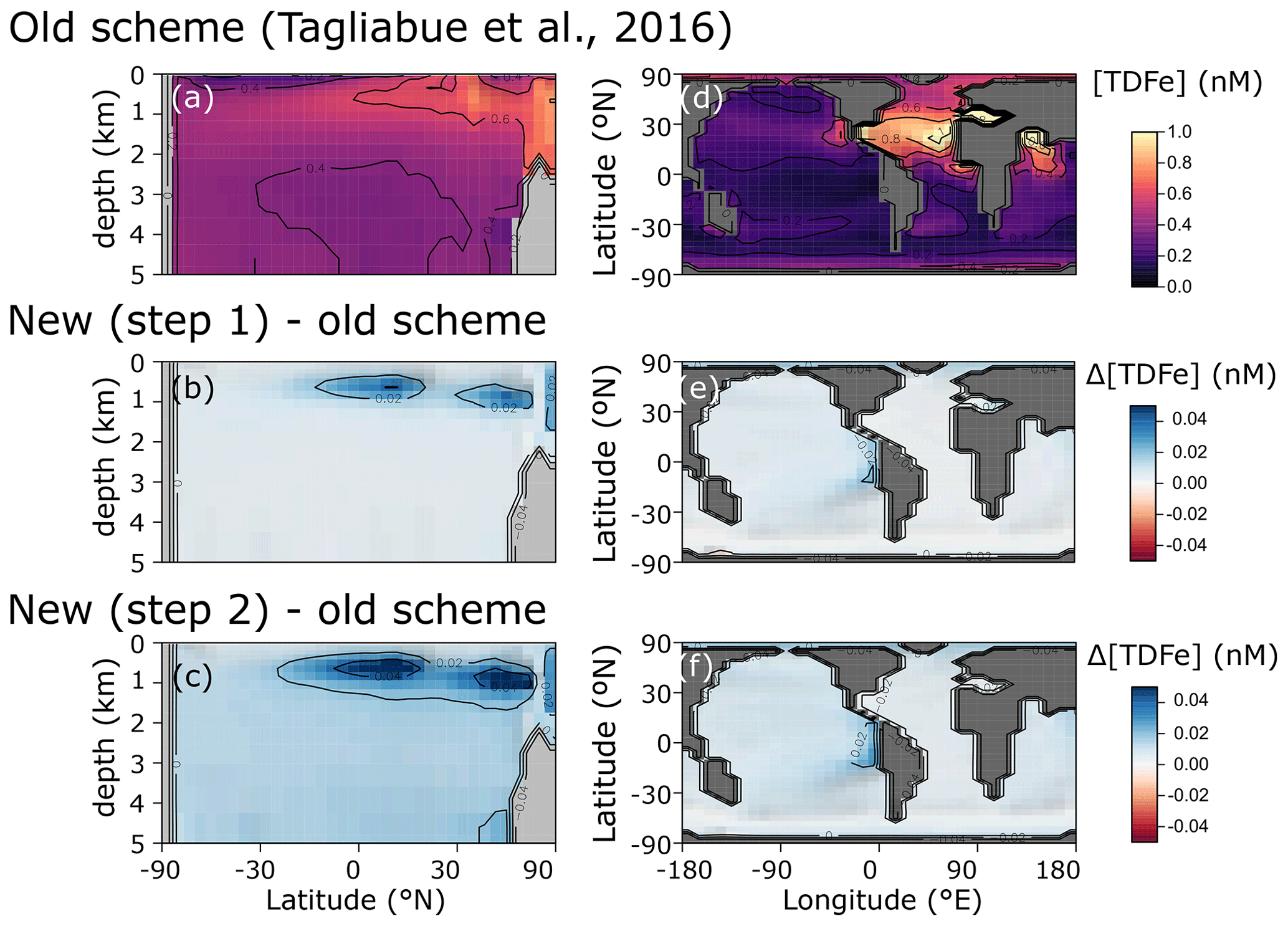
Figure 6Comparison of total dissolved Fe concentrations ([TDFe] = [Fe3+] + [Fe2+]) between (a, d) the old cGEnIE scheme (Tagliabue et al., 2016), (b, e) the new scavenging scheme, and (c, f) the full new scheme. (a–c) Zonally averaged TDFe concentrations, (d–f) surface TDFe concentrations (all units: nM). (b, c, e, f) Positive values indicate that the new scheme has higher concentrations, and negative values indicate that the old scheme has higher concentrations.
The small differences in [TDFe] translate to a negligible increase in global export production (Table 5) and indicates that the differences in performance between the old and new cGEnIE Fe cycle scheme are relatively trivial in a modern and nearly fully oxygenated ocean. For both the new and the old scheme, the sink of iron is scavenging of its oxidized form and no FeS2 is formed (Table 5). Pyrite will only precipitate once FeS has passed its solubility threshold, which is ∼2 µM, and such concentrations are not reached in the modern ocean. Because the new scheme is more mechanistic, as it allows for reduction of Fe3+ in anoxic conditions, we believe our new extension will also be beneficial for studies of the modern iron cycle – in particular when addressing topics such as future ocean deoxygenation or intervals of the more recent geological past characterized by much more extensive OMZs than present.
Tagliabue et al. (2016)Table 5Comparison of selected model output for the old Fe scheme and the new Fe scheme.
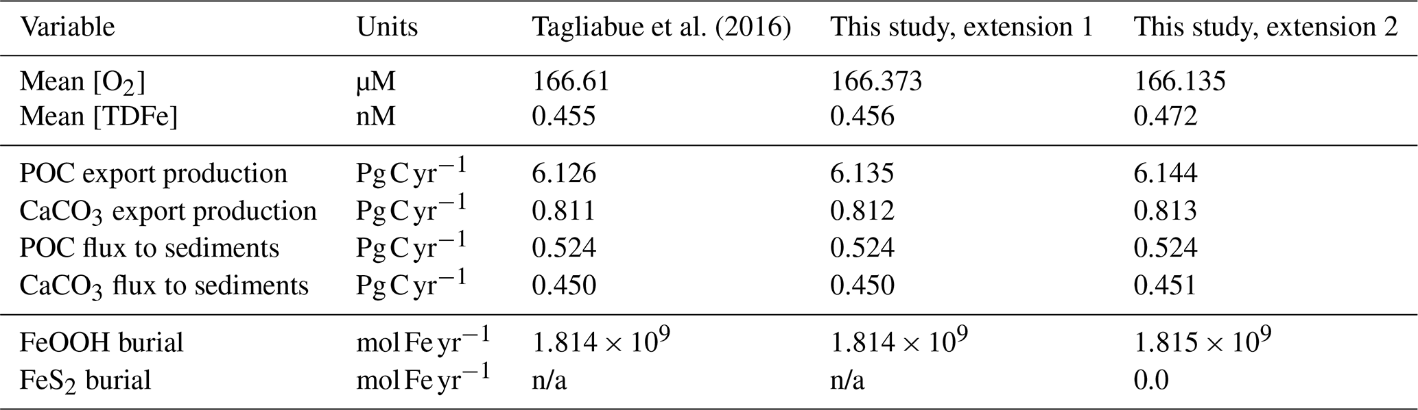
n/a: not applicable.
4.2 An anoxic ocean
For testing and characterizing the Fe–S cycle model developments under anoxic conditions, we configure cGENIE with a single continent that runs from pole to pole (Figs. 2c, 3a). Each model experiment is initialized from a homogeneous and static ocean, with an imposed constant atmospheric O2 concentration of 0.1 PAL (present atmospheric level, i.e. 21 000 ppm) and an atmospheric CO2 concentration of ∼16 PAL (5337.6 ppm). These atmospheric boundary conditions are chosen as broadly plausible for the Precambrian Earth system and deliberately preclude the formation of sea ice in order to simplify the resulting spatial tracer patterns in the ocean and their mechanistic interpretation. The model is run in a “closed” configuration for all elements (notably C and P), in which the ocean–atmosphere inventory for each element is always conserved. We chose to keep a closed configuration for C and P because this allows us to fix important boundary conditions (such as pCO2 and productivity) and look at the emerging ocean redox state under these conditions. An exception is made for Fe and S, which enter the surface ocean in the form of Fe2+ and and exit the ocean as FeOOH, FeS2, FeCO3, or Fe3Si2O5(OH)4. Fluxes of Fe and S are chosen to be in balance with respect to FeS2 burial () and to represent the best estimate of present-day weathering fluxes to the ocean (excluding reprocessing in inner-shelf sediment settings) ( mol yr−1, mol yr−1; Poulton and Raiswell, 2002; Raiswell and Canfield, 2012). Hydrothermal systems represent another potentially important flux of Fe to the ocean (Tagliabue et al., 2010; Conway and John, 2014; Lough et al., 2019), and this flux is likely to be elevated when ocean chemistry is pervasively anoxic and relatively low in (Kump and Seyfried, 2005). Our simulations therefore also include a hydrothermal flux of Fe2+, broadly comparable to a plausible input flux to Proterozoic oceans (15.1×10¹² mol yr−1; Thompson et al., 2019). This Fe2+ flux in our model set-up is equally distributed along a “hydrothermal ridge” located in the middle of the ocean (a straight line from k=9, l=3 to k=9, l=15; Fig. 2a). In order to balance the S:Fe flux ratio at 2:1 (see above), we must also specify a uniform surface flux of of 30.2×10¹² mol yr−1. This is an extremely high S flux and is unlikely to be realistic on long timescales. However, it allows us to quickly diagnose spatial patterns in reducing Fe–S cycling at steady state, without a priori introducing a bias towards ferruginous or euxinic redox states. We initialize the model with an average ligand concentration of 1 nM (comparable to the modern ocean) and a semi-arbitrary marine phosphate inventory that is 50 % of today in order to reduce marine primary productivity (as productivity in the Precambrian ocean was likely lower than today; Crockford et al., 2018; Ozaki et al., 2019), and we run the ocean circulation to steady state for 20 000 years for each individual experiment and present model output from the 20 000th year of integration. It is important to emphasize that the idealized configuration we implement here is not meant to represent any specific period or event in Earth's history, but is rather meant to serve as a broadly plausible and computationally efficient set of boundary conditions for testing the extended model code.
The sea surface temperature and ocean circulation generated by our configuration of cGENIE are shown in Fig. 3. Sea surface temperatures vary from ∼40 ∘C at the Equator to <10 ∘C at the poles (Fig. 3c). The barotropic streamfunction shows a large degree of symmetry (Fig. 3d), whereas the overturning patterns are skewed to the Southern Hemisphere, with a strong anticlockwise circulation at around −60∘ N (Fig. 3e). The overturning streamfunction shows strong upwelling at the Equator and deepwater mixing at the poles (Fig. 3e). The wind stress at the Equator drives surface waters towards the west, which will lead to stronger upwelling on the west side of the continent. The redox patterns discussed below will reflect these two main features: (i) upwelling at the Equator, in particular at the west side of the continent, and (ii) deepwater mixing at the poles.
In the following section, we briefly discuss the spatial model output and modelled redox cycling for our baseline configuration. Precipitation fluxes of oxidized Fe3+ are specified according to the scavenging scheme (Eq. 11). We focus here on (i) three depth slices of particle sinking fluxes of POC, FeOOH, FeS2, and Fe3Si2O5(OH)4 (Fig. 7; FeCO3 fluxes were negligible and are not shown); (ii) the average and three vertical longitudinal slices of O2, dissolved Fe3+, Fe2+, and dissolved ΣH2S (Fig. 8); and (iii) an overview of globally averaged reaction rates and iron mineral burial fluxes (Table 6).
The POC flux decreases with depth in the model from a maximum of ∼10 immediately below the surface layer to near-zero values at the seafloor (Fig. 7a–c). The spatial pattern of solid-FeOOH flux (following the scavenging scheme described earlier – see Sect. 3.1.1) matches the POC flux pattern immediately below the surface layer, with higher values at the Equator and poles (dark blue shading in Fig. 7d). Most of this FeOOH is reduced in anoxic subsurface layers, and the flux declines with depth. However, at the poles where deep convection allows for greater oxygen (and Fe3+) penetration into the ocean interior (Fig. 8a–h), sinking particles have more time to continue to scavenge and accumulate Fe3+, and the flux increases with depth (Fig. 7e, f). The maximum FeOOH flux at the seafloor reaches ∼300 (Fig. 7f), comparable to that observed in typical modern ocean margin sediments (see e.g. van de Velde and Meysman, 2016). Fluxes of FeS2 reach their maximum near the seafloor (where a source of deep Fe2+ is supplied via the imposed hydrothermal flux), with maximum fluxes similar to those of FeOOH (Fig. 7g–i). The spatial pattern of Fe3Si2O5(OH)4 formation is very similar to FeS2, but the fluxes are several orders of magnitude lower (Fig. 7j–l). Fluxes of FeCO3 were near zero everywhere (data not shown), consistent with recent work suggesting that water-column precipitation of FeCO3 is difficult to achieve, even in iron-dominated oceans (Jiang and Tosca, 2019; Tosca et al., 2019). The negligible FeCO3 fluxes are at odds with Fe-speciation data for Precambrian rocks showing that an important fraction of sedimentary Fe consists of reduced non-sulfurized Fe minerals (Sperling et al., 2015). Our results indicate that these minerals are most likely formed during sedimentary diagenesis, emphasizing the potential importance of processes below the sediment–water interface in structuring Fe-speciation signals in Earth's rock record. Future development will thus include a representation of sedimentary Fe cycling in the sedimentary module OMEN-SED (Hülse et al., 2018).

Figure 7Model output of (a)–(c) particulate organic carbon flux (JPOC), (d)–(f) solid-iron oxide flux (JFeOOH), (g)–(i) pyrite flux (), and (j)–(l) greenalite flux () for an ocean with 50 % of the modern phosphate inventory. JPOC is given in , JFeOOH and are given in , and is given in . The siderite flux () was near zero everywhere and is not shown here.
We additionally find that even in an idealized ocean with a simple symmetrical continental configuration, complex spatial patterns emerge in the Fe–S redox chemistry (Fig. 8). For instance, the poles are more well-ventilated, allowing oxygenated conditions and persistence of Fe3+ to a few kilometres of depth in our benchmark simulation (Fig. 8a–h). The concentrations of Fe3+ are much higher than the nanomolar and picomolar concentrations we observe in the ocean today (Tagliabue et al., 2016), which is a consequence of much higher rates of iron delivery to the surface ocean (through upwelling of reduced Fe2+) that allows Fe3+ to accumulate to higher concentrations before it is eventually scavenged. Our model predicts concentrations in the hundreds of nanomolar range (up to micromolar at the oxic–anoxic interface), which compares well to oxic water layers overlying anoxic deep water (Taillefert and Gaillard, 2002; Crowe et al., 2008). Note that this Fe3+ is likely in colloidal or nanoparticulate form and not truly dissolved. At eastward latitudes, deep convection at the poles is less intense, and upwelling on the eastward edge of the ocean leads to higher export production, which subsequently leads to build-up of reduced Fe2+ and ΣH2S (Fig. 8l and p). Dissolved Fe2+ reaches higher concentrations in the deeper ocean, largely as a result of deep hydrothermal inputs (Fig. 8i–l), whereas the highest ΣH2S concentrations are spatially constrained to areas of more intense POC degradation along the Equator, just below the oxic zone (Fig. 8m–p).
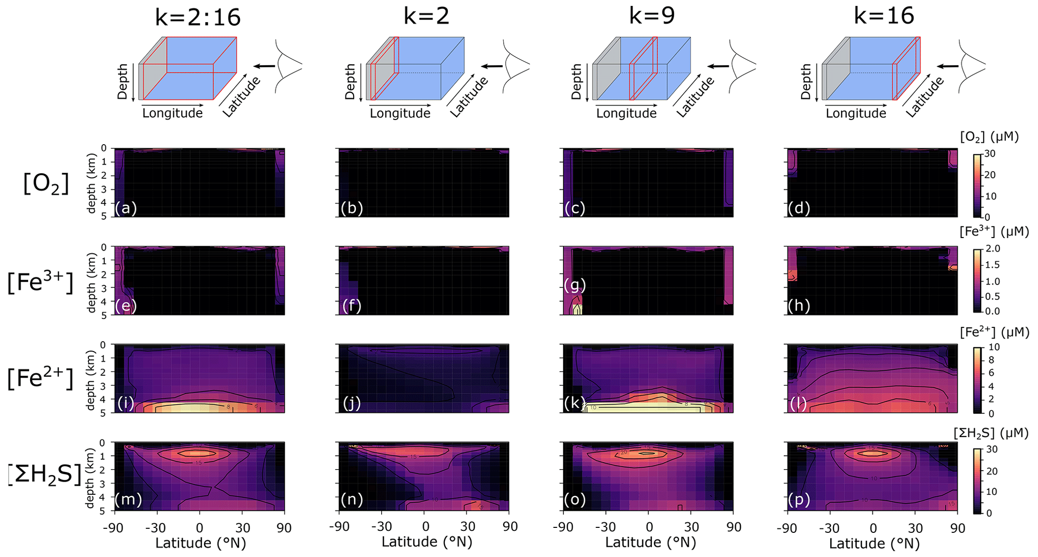
Figure 8Model output of (a)–(d) dissolved oxygen (O2), (e)–(h) dissolved ferric iron (Fe3+), (i)–(l) total dissolved ferrous iron (Fe2+), and (m)–(p) total dissolved sulfide (ΣH2S) for an ocean with 50 % of the modern phosphate inventory (all concentrations: µM).
Because pervasive anoxia is not present in modern open-ocean environments (see above), evaluation of the realism of our globally integrated reaction rates must rely on comparison to modern process analogues for ancient oceans (e.g. anoxic lake and restricted marine systems). Though we consider this a valid approach, it must be borne in mind that the transport processes in particular are very different in stratified lacustrine and marine systems, and there are reasons to assume that the biogeochemical dynamics of these systems will not strictly map onto pervasively anoxic open-ocean environments. However, though the absolute values are not directly comparable, we can qualitatively compare our results with rates derived from anoxic lake systems. For instance, our default model suggests that DIR is a negligible contributor to POC mineralization (Table 6), consistent with previous observations from ferruginous Lake Matano and the euxinic Black Sea (Konovalov et al., 2006; Crowe et al., 2011). However, Crowe et al. (2011) found that rates of DIR were roughly an order magnitude lower than those of methanogenesis, whereas we find that DIR is 5 orders of magnitude less important than all other mineralization pathways (Table 6). One possible reason for this discrepancy is the importance of sediment recycling in the natural lake system, which our model does not currently represent. Due to the shallower water column (e.g. ∼300 m in Lake Matano versus 5000 m in our idealized ocean), there is a much stronger coupling between sedimentary processes (i.e. the recycling of Fe as a benthic flux) and water-column processes. Indeed, when the total rate of DIR is corrected for iron recycling occurring in sediments within Lake Matano the importance of DIR decreases by several orders of magnitude (Crowe et al., 2008). Additionally, cGENIE treats POC as a concentration assumed to be uniformly dispersed throughout a grid cell, meaning that POC and FeOOH concentrators used in reaction calculation will not take into account the reality of particulate matter being locally aggregated and highly concentrated as it sinks.
Table 6Globally integrated reaction rates and burial fluxes for our benchmark simulation.
Our model predicts a globally integrated FIO rate of (Table 6), which is lower than rates estimated for anoxic lakes (12– ; Crowe et al., 2008; Walter et al., 2014). However, rates measured near the oxycline ( ) are comparable to rates measured in anoxic lake systems. Interestingly, more than half of the ΣH2S is re-oxidized via SMI (Table 6), which indicates that Fe is able to act as a relatively efficient intermediate between ΣH2S oxidation and O2 reduction. This also occurs in the Black Sea, where metal oxides are responsible for ∼60 % of the sulfide re-oxidation (Konovalov et al., 2006).
Isotope patterns
Figure 9a–e show the modelled stable Fe isotope patterns for all key Fe-bearing dissolved and solid-phase species (with the exception of FeCO3, which is a negligible component in our benchmark simulation). In our model simulations, all dissolved Fe that enters the ocean is assigned an isotope signature of 0.0 ‰. This allows us to observe the isotope fractionation of all Fe phases relative to the Fe that entered the ocean (Fig. 10a). The dissolved iron phases show similar isotopic signatures (∼1.1 ‰; Figs. 9a, b, 10a), which can be explained by the large amount of isotopically light FeS2 burial (Fig. 10a) that drives to heavier values. Note that the very heavy values only occur in the ocean interior, where the concentration of Fe3+ is virtually zero (Fig. 8e–h). The isotope signature of buried oxidized iron (FeOOH) is around 1.8 ‰ heavier than the Fe that entered the ocean, whereas the major burial fraction of reduced iron (FeS2) has an isotope signature that is ∼1 ‰ lighter, which reflects their relative importance as an Fe burial phase (Figs. 9c, e, 10a). These isotope values are broadly comparable to phase-specific stable Fe isotope observations from ancient sedimentary rocks (Heard and Dauphas, 2020). Similarly, Fig. 9f–g show the modelled stable S isotope patterns for all key S-bearing dissolved and solid-phase species.
All dissolved S that enters the ocean is assigned an isotope signature of 0.0 ‰. Sulfate is isotopically enriched relative to its input value (∼3.5 ‰; Figs. 9f, 10b), and this difference compares well to the geological record ( is ∼5 ‰ heavier than its input value; Canfield and Farquhar, 2009). Additionally, free sulfide is isotopically lighter than sulfate ( ‰ on a global scale; up to ‰ locally), while buried FeS2 expresses an isotope signature of ‰ (Fig. 10b). Our baseline simulation thus suggests that the expressed isotope fractionation between and FeS2 is only around 6.5 ‰, which is roughly consistent with what is observed in the geological record (Canfield and Farquhar, 2009). Therefore, we conclude that our model has strong potential for tracking iron and sulfur isotope signatures for comparison with Earth's rock record.
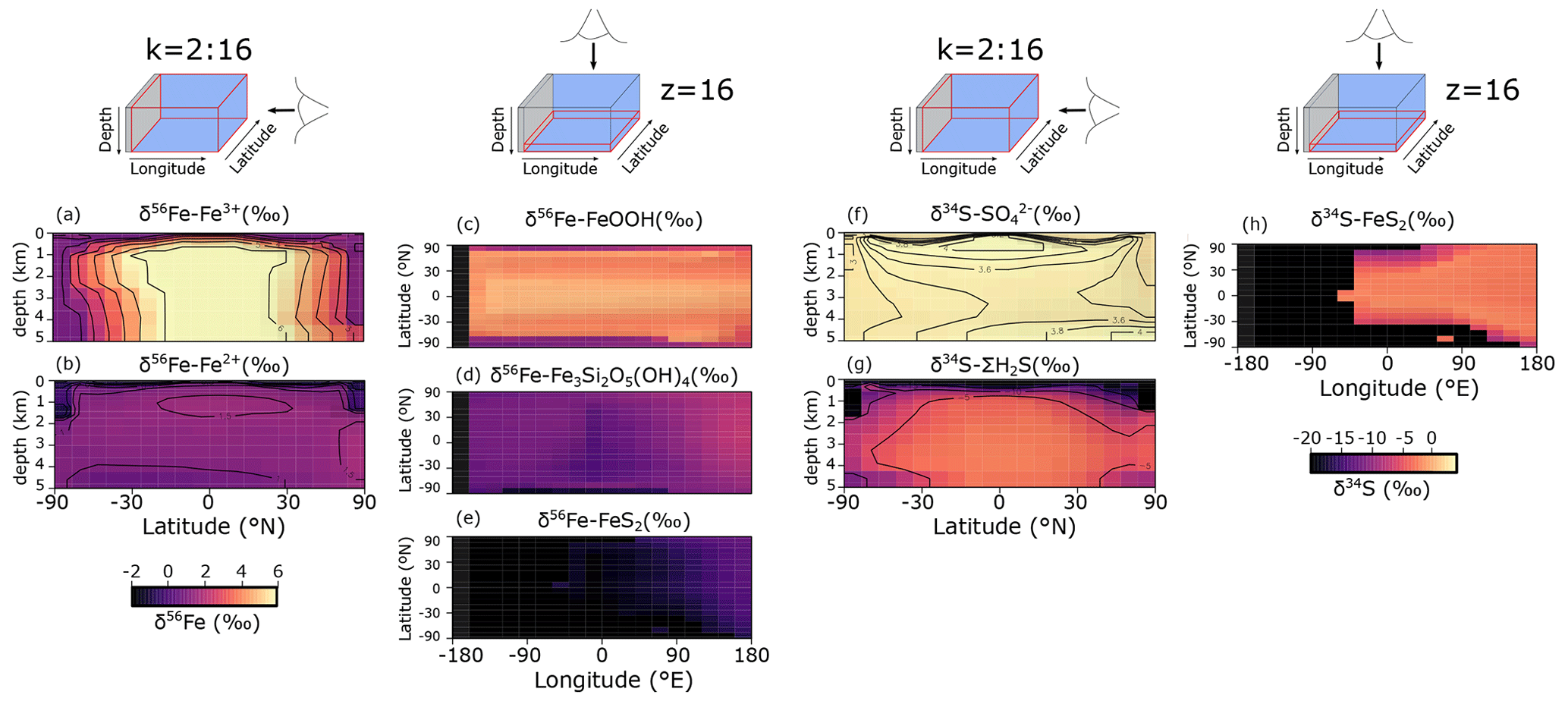
Figure 9(a–e) Modelled stable Fe isotope signatures of key dissolved and solid-phase Fe species. Shown are zonally averaged values for (a) dissolved ferric Fe () and (b) dissolved ferrous iron (), as well as the isotope compositions at the seafloor of (c) iron oxides (δ56Fe−FeOOH), (d) greenalite (δ56Fe−Fe3Si2O5(OH)4), and (e) pyrite (δ56Fe−FeS2) for an ocean with 50 % of the modern phosphate inventory. All values are in per mille relative to IRMM-14. (f–g) Modelled stable S isotope signatures of key dissolved and solid-phase S species. Shown are zonally averaged values for (f) sulfate () and (g) dissolved free sulfide (δ34S−ΣH2S), as well as (h) the isotope composition at the seafloor of pyrite (δ34S−FeS2). All values are in per mille relative to VCDT.
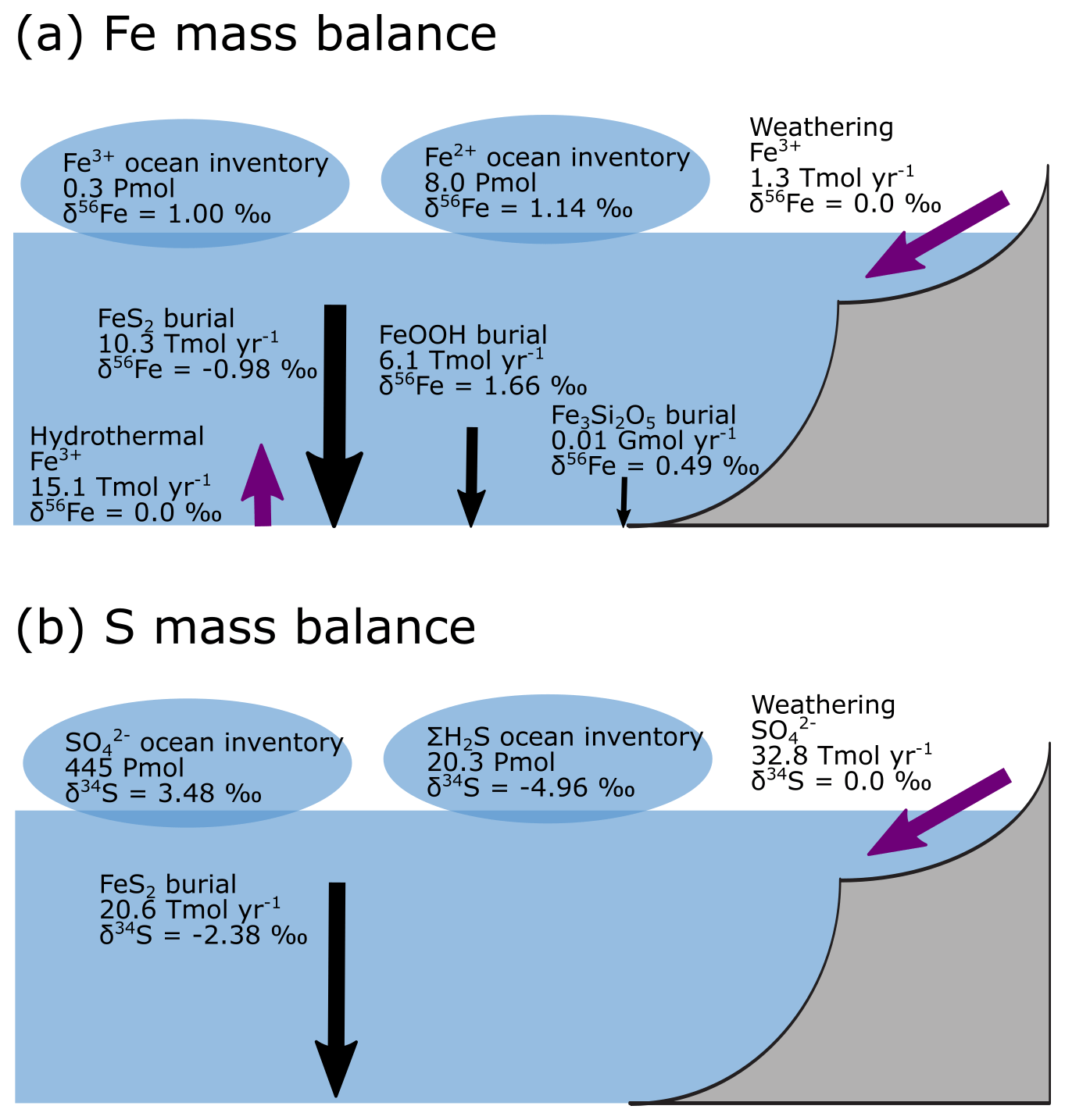
Figure 10Isotope mass balance for the (a) 56Fe and (b) 34S systems from our baseline simulation. Purple arrows are influxes, and black arrows are outfluxes. Bubbles represent the whole ocean inventory. Note that in our simulation, the S system is not in steady state (because FeS2 burial is too low).
4.3 Sensitivity analysis
We evaluate model output sensitivity to four key parameters of our modelled iron–sulfur cycle (K0,FeOOH, Ki,FeOOH, kSMI,s, kPyP) using the elementary effect test (EET; Morris, 1991). These parameters were chosen because they are either unconstrained by laboratory experiments (K0,FeOOH, Ki,FeOOH; Sect. 3.1.2), represent a complex mixture of different iron minerals with different reactivities (kSMI,s; Poulton et al., 2004), or are expected to have a strong and potentially difficult to forecast influence on other reactions (kPyP; van de Velde et al., 2020b). Other parameters introduced in the model are either relatively well-constrained by laboratory studies and calibrated on field data (kCSO, kFIO; Millero et al., 1987a, b; Ridgwell et al., 2007), have been calibrated extensively in previous work (kscav; Tagliabue et al., 2016), or are likely to be of secondary importance to the iron–sulfur cycle (kAFC, bAFC, kgreenalite, bgreenalite).
The EET method estimates global sensitivity by calculating the mean of r finite differences (“elementary effects”) (Pianosi et al., 2016):
where represents the jth value of the ith parameter, represents the variation of the ith parameter, f() is the model output for a given set of parameters, and ci is a scaling factor. A higher mean value of Si indicates that a given model output is more sensitive to variations in parameter i. The standard deviation can also be calculated, with a high standard deviation indicating that a parameter interacts with others because its sensitivity changes across the variability space (inlay in Fig. 11; Pianosi et al., 2016).
Table 7Sensitivity range and baseline values of each parameter tested. Note that the units are not identical to the units used in the user configuration files for the cGENIE model. A table with the parameter units converted to cGEnIE units is included in Appendix A.
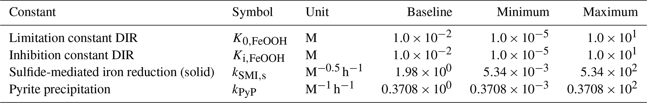
We use the EET method, as implemented within the Sensitivity Analysis For Everyone (SAFE) toolbox (Pianosi et al., 2015), to investigate the four chosen model parameters across the ranges specified in Table 7. We vary the limitation and inhibition constants K0,FeOOH and Ki,FeOOH over 6 orders of magnitude around the default (baseline) value due to the high uncertainty associated with these parameters. The lower bound of the reaction constant of solid iron oxide with sulfide (kSMI,s) is defined as the reactivity of hematite ( ; Poulton et al., 2004), and the upper bound is taken to be 5 orders of magnitude higher (5.34×10² , which is comparable to freshly precipitated hydrous ferric oxide). We test the pyrite precipitation constant (kPyp) across a range between and 0.3708×10² , which corresponds to the range of kinetic constants commonly used in diagenetic models (see e.g. Van Cappellen and Wang, 1996; Meysman et al., 2003; Dale et al., 2009; van de Velde et al., 2020a). Our sensitivity ensemble consists of 100 individual model experiments using a Latin hypercube sampling approach (using the SAFE toolbox; Pianosi et al., 2015) to select random starting points and parameter variations Δi. For more information on the sampling strategy we refer the interested reader to Campolongo et al. (2011).
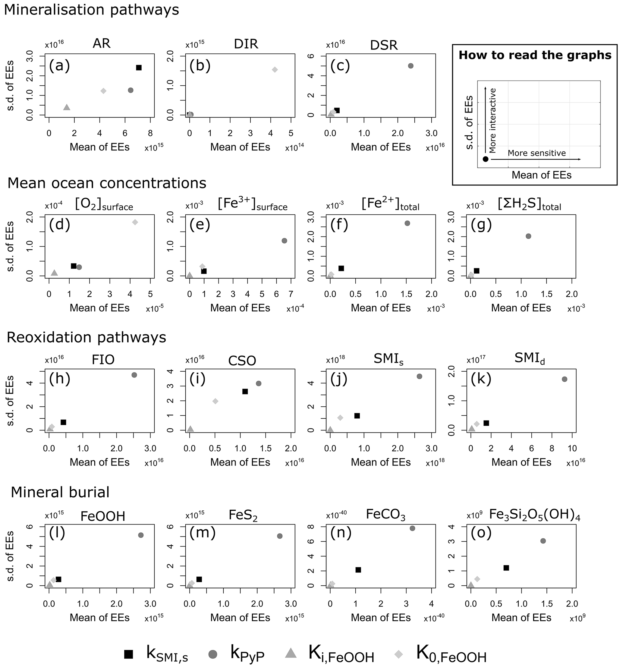
Figure 11Sensitivity analysis of the four key parameters of the iron–sulfur cycle for a range of different outputs. Inset shows how to read the graph; points that plot more to the right indicate that the specific output is more sensitive to changes in parameter values, and points that plot higher indicate that the parameter is more interactive with other parameters. Data processing was done with the SAFE toolbox of Pianosi et al. (2015).
The EET analysis suggests that changes in K0,FeOOH can significantly impact DIR, whereas the inhibition constant Ki,FeOOH has a relatively minor impact on model output (Fig. 11). This is expected, as both parameters act only on the mineralization pathways (Eq. 10). It is also consistent with some of the literature on anoxic systems, which suggests that in many cases the majority of iron reduction in the water column is coupled to sulfide (Mikucki et al., 2009). Even though both K0,FeOOH and Ki,FeOOH are the least constrained by experimental results (see Sect. 3.1.2), the EET analysis indicates that they are relatively unimportant for the overall model output despite their impact on DIR. In contrast, kPyP and kSMI,s both exerted a more notable impact on model output across a range of diagnostics (Fig. 11). In particular, kPyP had a significant impact across all model output diagnostics analysed here in terms of both model sensitivity and interactivity with other parameters (Fig. 11). Because pyrite precipitation controls the inventories of both dissolved Fe2+ and dissolved ΣH2S, reducing or increasing the kinetic precipitation parameter will affect the ambient concentrations, re-oxidation pathways, and eventual mineral burial for all phases across the Fe–S system.
Unfortunately, an elementary effect test gives no quantitative metric to evaluate the magnitude with which a parameter affects overall model outcome. Therefore, to illustrate the quantitative impact of the possible parameter choices, we ran a separate set of experiments in which we changed a parameter from its baseline value to its lower and upper bound whilst keeping the other three parameters at their baseline values (Table 7).
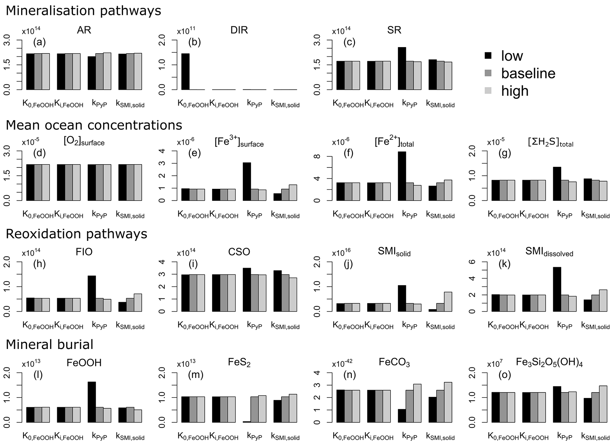
Figure 12Global model output for the three different values of the four key parameters (K0,FeOOH, Ki,FeOOH, kPyP, and kSMI,s). Low, baseline, and high values are given in Table 7. Panels (a)–(c) and (h)–(n) are in moles per year (mol yr−1), and panels (d)–(g) are in moles per kilogramme (mol kg−1).
Figure 12 reveals that AR, DSR, mean surface O2 concentrations, and CSO are relatively insensitive to parameter choices (Fig. 12a, c, d, i). Dissimilatory iron reduction is only important when K0,FeOOH is set at its lowest value, and even then it is 3 orders of magnitude smaller than AR or SR (Fig. 12a–c). Consistent with the EET analysis (Fig. 11), K0,FeOOH and Ki,FeOOH have no influence on the model output aside from the magnitude of DIR, which in itself is of less importance than the mineralization pathway (Fig. 12b and Sect. 4.2). In contrast, changes in the pyrite precipitation constant kPyP impact several model outputs. When pyrite precipitation rates are elevated, Fe2+ and ΣH2S are removed from local seawater more rapidly, which results in the following:
-
a decreased build-up of Fe2+ and ΣH2S in the ocean interior (Fig. 12f, g), leading to
-
a decrease in both aerobic and anaerobic re-oxidation pathways (FIO, SMId, and SMIs; Fig. 12h–k), which then results in
-
more O2 available for aerobic respiration at the expense of less thermodynamically favourable electron acceptors (i.e. AR increases and DSR decreases; Fig. 12a, c),
-
a decrease in Fe3+ concentrations in the surface ocean (Fig. 12e), and
-
less burial of FeOOH, increasing the burial of reduced iron minerals (Fig. 12l–n).
The effect on greenalite burial is non-linear (Fig. 12o), which indicates that at higher values of kPyP, pyrite precipitation is competing with greenalite precipitation. Overall, our sensitivity analysis suggests that kPyP is an important parameter for the model output and should be chosen with care. Fortunately, pyrite precipitation has been well-studied in laboratory experiments (Rickard, 1997, 2006), with the result that our baseline value for this parameter is relatively well-constrained.
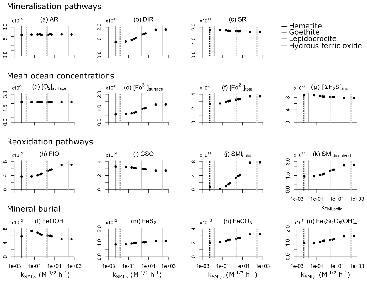
Figure 13Global model output for a range of kSMI,s values (units are ). Lines indicate experimental reactivity parameters as presented in Poulton et al. (2004). Panels (a)–(c) and (h)–(n) are in moles per year (mol yr−1), and panels (d)–(g) are in moles per kilogramme (mol kg−1). Note that the x axis is logarithmic.
The fourth parameter, which also influences the model output, is the reactivity parameter of solid iron oxides (kSMI,s). Here, the parameter choice is more complex. Laboratory experiments have shown that different iron oxide minerals exhibit a wide reactivity range (spanning several orders of magnitude) (Canfield et al., 1992; Poulton et al., 2004). Therefore, we explore the sensitivity of this parameter in more detail using a range of measured reactivity constants by Poulton et al. (2004) whilst keeping all other parameters at their baseline values (Fig. 13). Increasing the reactivity of particulate FeOOH does the following:
-
increases the anaerobic re-oxidation reaction of sulfide with FeOOH (SMIs) at the expense of the aerobic re-oxidation reaction (CSO) (Fig. 13i, j), which then leads to
-
an increase in the Fe2+ inventory and a decrease in the ΣH2S inventory (Fig. 13f, g); more Fe2+ leads to
-
more FIO and thus a higher surface Fe3+ concentration and more re-oxidation of ΣH2S with dissolved Fe3+ (SMId; Fig. 13e, h, k).
-
Because of the higher reactivity of the FeOOH particles, less FeOOH is buried, and more reduced Fe minerals are buried (Fig. 13l–o).
Although it is clear that changing kSMI,s impacts model output, the overall magnitude of the effect is moderate when compared to changing kPyP. Nevertheless, the choice of kSMI,s is critical. We choose a baseline reactivity value (Table 3) comparable to lepidocrocite for several reasons. Firstly, we assume all Fe3+ that is not scavenged represents a “colloidal” pool, with a reactivity similar to that of hydrous ferric oxide. When Fe3+ becomes scavenged (and is thus in solid state), it has likely undergone some ageing, and it will be less reactive than hydrous ferric oxide. Secondly, any FeOOH that does not react in the water column will end up in the sediment and will, at least in part, be recycled back to the water column (even under oxic conditions; Dale et al., 2015). Our model currently lacks a sedimentary iron cycle (see Sect. 5) and would thus tend to underestimate the overall importance of the iron cycle were we to select a reactivity constant that is too low. Finally, field evidence suggests that FeOOH that is freshly precipitated is highly reactive (Picard et al., 2015; Beam et al., 2018), and thus iron precipitating from the surface ocean is expected to react on relatively short timescales. Any FeOOH minerals that would resist reduction passing through a sulfidic water column are likely unreactive and are thus presumably inert on early diagenetic timescales. Indeed, iron oxide minerals in sediments underlying euxinic water columns tend to show no depth trend, indicating that very little iron reduction is occurring at depth in such systems (see e.g. Xiong et al., 2019). Taken together, these observations support the presumption that once Fe3+ is scavenged, its reactivity is less than hydrous ferric oxide but higher than that of goethite, motivating our default kSMI,s value. Nevertheless, the value used for this parameter should be considered carefully depending on the model application and assumed boundary conditions.
The principal aim of this paper is to provide a detailed description of our extension of the cGENIE biogeochemistry module to include coupled anoxic Fe and S biogeochemical cycles. Because direct tuning with actual measured concentrations and rates is not possible, we have relied heavily on kinetic constants and solubility values extracted from laboratory incubations. While care should be exercised in the application of these kinetic constants to reactions under in situ conditions, our sensitivity analysis indicates that our key model results are robust across a wide range of possible parameter values. In addition, our proposed baseline parameterization yields reaction rates, concentrations, burial fluxes, and stable Fe isotope compositions that broadly compare well to both field measurements of process analogues for ancient ocean systems (i.e. anoxic lakes) and observations from the geologic record. Therefore, we believe that our model description of the anoxic Fe–S cycle is a valuable tool and an important step forward in simulating ocean redox landscapes during periods of Earth's history in which the ocean interior was pervasively anoxic. However, below we highlight some important limitations to our current model architecture and also give some examples of possible future developments.
Most notably, our model is currently unable to resolve any sedimentary processes that would contribute to the global iron cycle (see e.g. Dale et al., 2015). In particular, the model does not include a representation of benthic iron reduction and recycling back into the water column. Building on the improvements in the biogeochemistry of cGENIE described here, in the future we plan to extend the organic-matter-enabled sediment component of cGENIE (OMEN-SED; Hülse et al., 2018) to include an explicit representation of the benthic iron cycle. We anticipate that this will both improve the realism of tracer fields within the ocean interior and make comparisons between predicted sedimentary signals and observations from Earth's sedimentary rock record more accurate and robust. Second, there are likely to be important mechanistic links between the biogeochemistry of Fe and S within the ocean and the local and global recycling and bioavailability of key nutrient species for the biosphere (Bjerrum and Canfield, 2002; Laakso and Schrag, 2014; Jones et al., 2015; Reinhard et al., 2017). Future work will thus also focus on explicitly coupling the anoxic Fe and S biogeochemistry to the phosphorus (P) and nitrogen (N) cycles, in particular the scavenging and remobilization of P under different redox states and the impact of dissolved Fe availability on nitrogen fixation. The modularity of cGENIE also allows the substitution of an explicit plankton ecological model (ECOGEM) for the default biological export scheme (Ward et al., 2018), enabling the exploration of feedbacks between marine ecosystems, nutrient availability, and ocean redox conditions (Reinhard et al., 2020b). Lastly, future work will seek to include other redox-sensitive proxies and bio-essential elements such as molybdenum, uranium, or vanadium (Tribovillard, 2006) within the model code, which will further extend the applicability of our model and help validate it against observations from modern anoxic systems and the geologic record.
Table A1List of kinetic constants for the reactions included in the cGENIE model – converted to cGEnIE units.
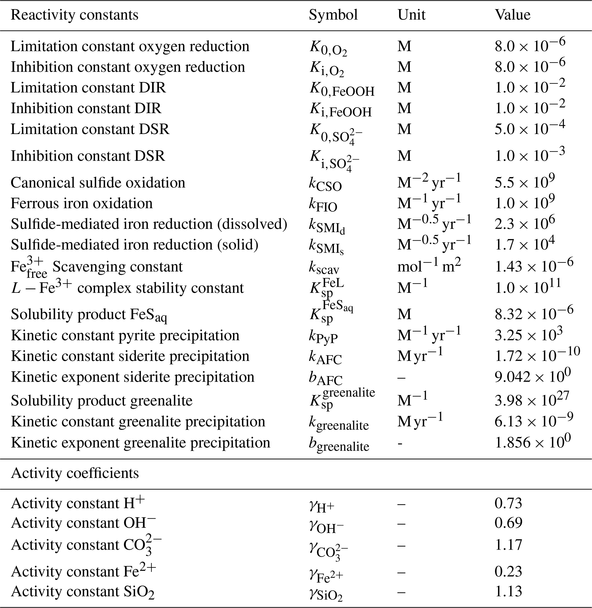
Table A2Sensitivity range and baseline values of each parameter tested – converted to cGEnIE units.
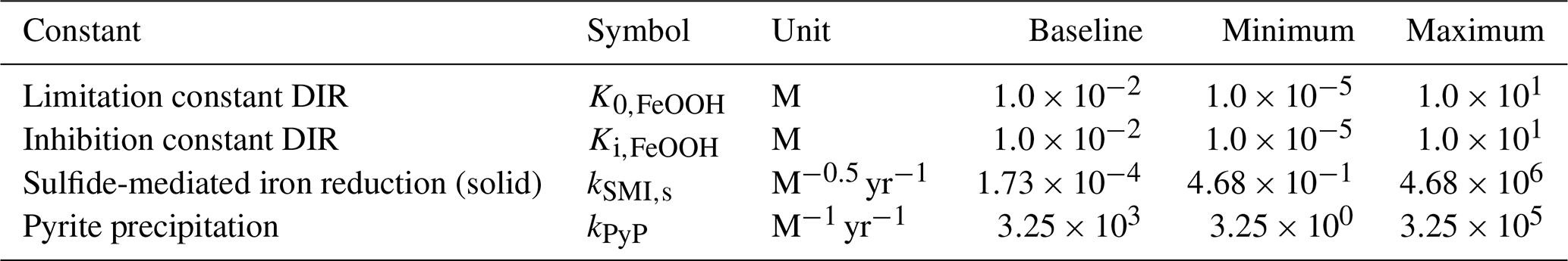
The code for the version of the “muffin” release of the cGENIE Earth system model used in this paper is tagged as v0.9.21 and is assigned a DOI: https://doi.org/10.5281/zenodo.4651390 (Ridgwell et al., 2021b). The code is hosted on GitHub and can be obtained by cloning
https://github.com/derpycode/cgenie.muffin,
changing the directory to cgenie.muffin, and then checking out the specific release:
$ git checkout v0.9.21.
Configuration files for the specific experiments presented in the paper can be found in the following directory.
genie-userconfigs/MS/vandeveldeetal.GMD.2021
Details of the experiments, plus the command line needed to run each one,
are given in the readme.txt file in that directory. All other configuration files and boundary conditions are provided as part of the code release.
A manual detailing code installation, basic model configuration, tutorials covering various aspects of model configuration and experimental design, plus results output and processing is assigned a DOI: https://doi.org/10.5281/zenodo.4651394 (Ridgwell et al., 2021a). The LaTeX source of the manual, along with a pre-built PDF format
version, can be obtained by cloning the following.
https://github.com/derpycode/muffindoc
No data sets were used in this article.
SJvdV and AR developed the model with input from all authors. CTR provided geological context. SJV and DH ran the sensitivity tests and analysed the output. SJvdV wrote the paper with input from all authors.
The authors declare that they have no conflict of interest.
This research has been supported by the Belgian American Educational Foundation (postdoctoral fellowship), the National Aeronautics and Space Administration (Nexus for Exoplanet System Science), the NASA Astrobiology Institute (NASA postdoctoral programme fellowship, administered by the Universities Space Research Association under contract with NASA), and the Simons Foundation (postdoctoral fellowship in marine microbial ecology, award 653829).
This paper was edited by Andrew Yool and reviewed by three anonymous referees.
Adloff, M., Ridgwell, A., Monteiro, F. M., Parkinson, I. J., Dickson, A., Pogge von Strandmann, P. A. E., Fantle, M. S., and Greene, S. E.: Inclusion of a suite of weathering tracers in the cGENIE Earth System Model – muffin release v.0.9.10, Geosci. Model Dev. Discuss. [preprint], https://doi.org/10.5194/gmd-2020-233, in review, 2020. a, b
Alcott, L. J., Mills, B. J. W., and Poulton, S. W.: Stepwise Earth oxygenation is an inherent property of global biogeochemical cycling, Science, 366, 1333–1337, https://doi.org/10.1126/science.aax6459, 2019. a
Balistrieri, L. S., Murray, J. W., and Paul, B.: The cycling of iron and manganese in the water column of Lake Sammamish, Washington, Limnol. Oceanogr., 37, 510–528, 1992. a
Balzano, S., Statham, P. J., Pancost, R. D., and Lloyd, J. R.: Role of microbial populations in the release of reduced iron to the water column from marine aggregates, Aquat. Microb. Ecol., 54, 291–303, https://doi.org/10.3354/ame01278, 2009. a, b
Beam, J. P., Scott, J. J., McAllister, S. M., Chan, C. S., McManus, J., Meysman, F. J. R., and Emerson, D.: Biological rejuvenation of iron oxides in bioturbated marine sediments, ISME J., 12, 1389–1394, https://doi.org/10.1038/s41396-017-0032-6, 2018. a
Beard, B. L., Johnson, C. M., Cox, L., Sun, H., Nealson, K. H., and Aguilar, C.: Iron isotope biosignatures, Science, 285, 1889–1892, 1999. a, b
Beard, B. L., Johnson, C. M., Skulan, J. L., Nealson, K. H., Cox, L., and Sun, H.: Application of Fe isotopes to tracing the geochemical and biological cycling of Fe, Chem. Geol., 195, 87–117, 2003. a
Bekker, A., Slack, J. F., Planavsky, N., Krapez, B., Hofmann, A., Konhauser, K. O., and Rouxel, O. J.: Iron Formation: The sedimentary product of a complex interplay among mantle, tectonic, oceanic, and biospheric processes, Econ. Geol., 105, 467–508, 2010. a
Berg, J. S., Michellod, D., Pjevac, P., Martinez-Perez, C., Buckner, C. R. T., Hach, P. F., Schubert, C. J., Milucka, J., and Kuypers, M. M. M.: Intensive cryptic microbial iron cycling in the low iron water column of the meromictic Lake Cadagno, Environ. Microbiol., 18, 5288–5302, https://doi.org/10.1111/1462-2920.13587, 2016. a
Berner, R. A.: Phosphate removal from sea water by adsorption on volcanogenic ferric oxides, Earth Planet. Sc. Lett., 18, 77–86, 1973. a
Berner, R. A.: Biogeochemical cycles of carbon and sulfur and their effect on atmospheric oxygen over phanerozoic time, Palaeogeogr. Palaeocl., 75, 97–122, 1989. a
Bjerrum, C. J. and Canfield, D. E.: Ocean productivity before about 1.9 Gyr ago limited by phosphorus adsorption onto iron oxides, Nature, 417, 159–162, https://doi.org/10.1038/417159a, 2002. a, b, c, d, e
Böttcher, M. E., Smock, A. M., and Cypionka, H.: Sulfur isotope fractionation during experimental precipitation of iron(II) and manganese(II) sulfide at room temperature, Chem. Geol., 146, 127–134, 1998. a
Brocks, J. J., Jarrett, A. J. M., Sirantoine, E., Hallmann, C., Hoshino, Y., and Liyanage, T.: The rise of algae in Cryogenian oceans and the emergence of animals, Nature, 548, 578–581, https://doi.org/10.1038/nature23457, 2017. a
Bullen, T. D., White, A. F., Childs, C. W., Vivit, D. V., and Schulz, M. S.: Demonstration of significant abiotic iron isotope fractionation in nature, Geology, 29, 699–702, 2001. a
Campolongo, F., Saltelli, A., and Cariboni, J.: From screening to quantitative sensitivity analysis – A unified approach, Comput. Phys. Commun., 182, 978–988, https://doi.org/10.1016/j.cpc.2010.12.039, 2011. a
Canfield, D. E.: A new model for Proterozoic ocean chemistry, Nature, 396, 450–453, 1998. a, b, c
Canfield, D. E.: Sulfur isotopes in coal constrain the evolution of the Phanerozoic sulfur cycle, P. Natl. Acad. Sci. USA, 110, 8443–8446, https://doi.org/10.1073/pnas.1306450110, 2013. a
Canfield, D. E. and Farquhar, J.: Animal evolution, bioturbation, and the sulfate concentration of the oceans, P. Natl. Acad. Sci. USA, 106, 8123–8127, 2009. a, b
Canfield, D. E. and Teske, A.: Late proterozoic rise in atmospheric oxygen concentration inferred from phylogenetic and sulphur-isotope studies, Nature, 382, 127–132, https://doi.org/10.1038/382127a0, 1996. a
Canfield, D. E., Raiswell, R., and Bottrell, S.: The reactivity of sedimentary iron minerals toward sulfide, Am. J. Sci., 292, 659–683, 1992. a, b
Canfield, D. E., Rosing, M. T., and Bjerrum, C.: Early anaerobic metabolisms, Philos. T. Roy. Soc. B, 361, 1819–1836, 2006. a
Canfield, D. E., Poulton, S. W., Knoll, A. H., Narbonne, G. M., Ross, G., Goldberg, T., and Strauss, H.: Ferruginous Conditions Dominated Later Neoproterozoic Deep-Water Chemistry, Science, 321, 949–952, 2008. a, b
Cao, L., Eby, M., Ridgwell, A., Caldeira, K., Archer, D., Ishida, A., Joos, F., Matsumoto, K., Mikolajewicz, U., Mouchet, A., Orr, J. C., Plattner, G.-K., Schlitzer, R., Tokos, K., Totterdell, I., Tschumi, T., Yamanaka, Y., and Yool, A.: The role of ocean transport in the uptake of anthropogenic CO2, Biogeosciences, 6, 375–390, https://doi.org/10.5194/bg-6-375-2009, 2009. a, b, c
Cloud, P.: A working model of the primitive Earth, Am. J. Sci., 272, 537–548, https://doi.org/10.2475/ajs.272.6.537, 1972. a
Colbourn, G., Ridgwell, A., and Lenton, T. M.: The Rock Geochemical Model (RokGeM) v0.9, Geosci. Model Dev., 6, 1543–1573, https://doi.org/10.5194/gmd-6-1543-2013, 2013. a
Conway, T. M. and John, S. G.: Quantification of dissolved iron sources to the North Atlantic Ocean, Nature, 511, 212–215, https://doi.org/10.1038/nature13482, 2014. a
Cosmidis, J., Benzerara, K., Morin, G., Busigny, V., Lebeau, O., Jézéquel, D., Noël, V., Dublet, G., and Othmane, G.: Biomineralization of iron-phosphates in the water column of Lake Pavin (Massif Central, France), Geochim. Cosmochim. Ac., 126, 78–96, https://doi.org/10.1016/j.gca.2013.10.037, 2014. a
Crichton, K. A., Wilson, J. D., Ridgwell, A., and Pearson, P. N.: Calibration of temperature-dependent ocean microbial processes in the cGENIE.muffin (v0.9.13) Earth system model, Geosci. Model Dev., 14, 125–149, https://doi.org/10.5194/gmd-14-125-2021, 2021. a, b
Crockford, P. W., Hayles, J. A., Bao, H., Planavsky, N. J., Bekker, A., Fralick, P. W., Halverson, G. P., Bui, T. H., Peng, Y., and Wing, B. A.: Triple oxygen isotope evidence for limited mid-Proterozoic primary productivity, Nature, 559, 613–616, https://doi.org/10.1038/s41586-018-0349-y, 2018. a
Crosby, S. A., Glasson, D. R., Cuttler, A. H., Butler, I., Turner, D. R., Whitfield, M., and Millward, G. E.: Surface areas and porosities of Fe(III)- and Fe(II)-derived oxyhydroxides, Environ. Sci. Technol., 17, 709–713, 1983. a
Crosby, S. A., Roden, E. E., Johnson, C. M., and Beard, B. L.: The mechanisms of iron isotope fractionation produced during dissimilatory Fe(III) reduction by Shewanella putrefaciens and Geobacter sulfurreducens, Geobiology, 5, 169–189, 2007. a
Crowe, S. A., O'Neill, A. H., Katsev, S., Hehanussa, P., Haffner, G. D., Sundby, B., Mucci, A., and Fowle, D. A.: The biogeochemistry of tropical lakes: A case study from Lake Matano, Indonesia, Limnol. Oceanogr., 53, 319–331, 2008. a, b, c, d, e, f
Crowe, S. A., Katsev, S., Leslie, K., Sturm, A., Magen, C., Nomosatryo, S., Pack, M. A., Kessler, J. D., Reeburgh, W. S., Roberts, J. A., González, L., Douglas Haffner, G., Mucci, A., Sundby, B., and Fowle, D. A.: The methane cycle in ferruginous Lake Matano, Geobiology, 9, 61–78, https://doi.org/10.1111/j.1472-4669.2010.00257.x, 2011. a, b
Crowe, S. A., Jones, C., Canfield, D. E., Paris, G., Adkins, J. F., Sessions, A. L., Katsev, S., Kim, S.-T., Zerkle, A. L., Nomosatryo, S., Fowle, D. A., and Farquhar, J.: Sulfate was a trace constituent of Archean seawater, Science, 346, 735–739, https://doi.org/10.1126/science.1258966, 2014. a
Dale, A. W., Brüchert, V., Alperin, M., and Regnier, P.: An integrated sulfur isotope model for Namibian shelf sediments, Geochim. Cosmochim. Ac., 73, 1924–1944, https://doi.org/10.1016/j.gca.2008.12.015, 2009. a
Dale, A. W., Nickelsen, L., Scholz, F., Hensen, C., Oschlies, A., and Wallmann, K.: A revised global estimate of dissolved iron fluxes from marine sediments, Global Biogeochem. Cy., 29, 1–17, 2015. a, b, c
Dehairs, F., Baeyens, W., and Goeyens, L.: Accumulation of Suspended Barite at Mesopelagic Depths and Export Production in the Southern Ocean, Science, 20, 1332–1335, https://doi.org/10.1126/science.258.5086.1332, 1990. a
Detmers, J., Bruchert, V., Habicht, K. S., and Kuever, J.: Diversity of sulfur isotope fractionations by sulfate-reducing prokaryotes, Appl. Environ. Microb., 67, 888–894, 2001. a
Diaz, R. J. and Rosenberg, R.: Spreading dead zones and consequences for marine ecosystems, Science 321, 926–929, 2008. a
Doney, S. C., Lindsay, K., Fung, I., and John, J.: Natural variability in a stable, 1000-yr global coupled climate-carbon cycle simulation, J. Climate, 19, 3033–3054, 2006. a, b
Edwards, N. and Marsh, R.: Uncertainties due to transport-parameter sensitivity in an efficient 3-D ocean-climate model, Clim. Dynam., 24, 415–433, 2005. a, b
Edwards, N. R. and Shepherd, J. G.: Bifurcations of the thermohaline circulation in a simplified three-dimensional model of the world ocean and the effects of interbasin connectivity, Clim. Dynam., 19, 31–42, 2002. a
Fakhraee, M., Hancisse, O., Canfield, D. E., Crowe, S. A., and Katsev, S.: Proterozoic seawater sulfate scarcity and the evolution of ocean-atmosphere chemistry, Nat. Geosci., 12, 375–380, https://doi.org/10.1038/s41561-019-0351-5, 2019. a
Ferreira, D., Marshall, J., and Campin, J.: Localization of Deep Water Formation: Role of Atmospheric Moisture Transport and Geometrical Constraints on Ocean Circulation, J. Climate, 23, 1456–1476, https://doi.org/10.1175/2009JCLI3197.1, 2010. a
Finster, K., Liesack, W., and Thamdrup, B.: Elemental sulfur and thiosulfate disproportionation by Desulfocapsa sulfoexigens sp. nov., a new anaerobic bacterium isolated from marine surface sediment, Appl. Environ. Microb., 64, 119–125, 1998. a
Froelich, P. N., Klinkhammer, G. P., Bender, M. L., Luedtke, N. A., Heath, G. R., Cullen, D., and Dauphin, P.: Early oxidation of organic matter in pelagic sediments of the eastern equatorial Atlantic: suboxic diagenesis, Geochim. Cosmochim. Ac., 43, 1075–1090, 1979. a
Fry, B., Gest, H., and Hayes, J. M.: 34S/32S fractionation in sulfur cycles catalyzed by anaerobic bacteria, Appl. Environ. Microb., 54, 250–256, 1988. a
Gomes, M. L. and Johnston, D. T.: Oxygen and sulfur isotopes in sulfate in modern euxinic systems with implications for evaluating the extent of euxinia in ancient oceans, Geochim. Cosmochim. Ac., 205, 331–359, 2017. a, b, c
Gorby, Y. A., Yanina, S., McLean, J. S., Rosso, K. M., Moyles, D., Dohnalkova, A., Beveridge, T. J., Chang, I. S., Kim, B. H., Kim, K. S., Culley, D. E., Reed, S. B., Romine, M. F., Saffarini, D. A., Hill, E. A., Shi, L., Elias, D. A., Kennedy, D. W., Pinchuk, G., Watanabe, K., Ishii, S., Logan, B., Nealson, K. H., and Fredrickson, J. K.: Electrically conductive bacterial nanowires produced by Shewanella oneidensis strain MR-1 and other microorganisms, P. Natl. Acad. Sci. USA, 103, 11358–11363, https://doi.org/10.1073/pnas.0604517103, 2006. a
Grotzinger, J. P. and Kasting, J. F.: New Constraints on Precambrian Ocean composition, J. Geol., 101, 235–243, 1993. a
Guilbaud, R., Butler, I. B., and Ellam, R. M.: Abiotic pyrite formation produces a large Fe isotope fractionation, Science, 332, 1548–1551, 2011. a
Guilbaud, R., Poulton, S. W., Butterfield, N. J., Zhu, M., and Shields-Zhou, G. A.: A global transition to ferruginous conditions in the early Neoproterozoic oceans, Nat. Geosci., 8, 466–470, https://doi.org/10.1038/NGEO2434, 2015. a, b
Guilbaud, R., Poulton, S. W., Thompson, J., Husband, K. F., Zhu, M., Zhou, Y., Shields, G. A., and Lenton, T. M.: Phosphorus-limited conditions in the early Neoproterozoic ocean maintained low levels of atmospheric oxygen, Nat. Geosci., 13, 296–301, 2020. a
Gustafsson, J. P.: Visual MINTEQ, version 3.1, KTH Royal Institute of Technology, Stockholm, Sweden, available at: https://vminteq.lwr.kth.se/ (last access: 20 December 2020), 2019. a, b
Halevy, I., Peters, S. E., and Fischer, W. W.: Sulfate burial constraints on the phanerozoic sulfur cycle, Science, 337, 331–334, https://doi.org/10.1126/science.1220224, 2012. a
Heard, A. W. and Dauphas, N.: Constraints on the coevolution of oxic and sulfidic ocean iron sinks from Archean-Paleoproterozoic iron isotope records, Geology, 48, 358–362, 2020. a, b
Henson, S. A., Sanders, R., Madsen, E., Morris, P. J., Le Moigne, F., and Quartly, G. D.: A reduced estimate of the strength of the ocean's biological carbon pump, Geophys. Res. Lett., 38, L04606, https://doi.org/10.1029/2011GL046735, 2011. a
Holland, H. D.: The Chemical Evolution of the Atmosphere and Oceans, Princeton University Press, Princeton, New Jersey, USA, 582 pp., 1984. a
Hülse, D., Arndt, S., Wilson, J. D., Munhoven, G., and Ridgwell, A.: Understanding the causes and consequences of past marine carbon cycling variability through models, Earth-Sci. Rev., 171, 349–382, https://doi.org/10.1016/j.earscirev.2017.06.004, 2017. a
Hülse, D., Arndt, S., Daines, S., Regnier, P., and Ridgwell, A.: OMEN-SED 1.0: a novel, numerically efficient organic matter sediment diagenesis module for coupling to Earth system models, Geosci. Model Dev., 11, 2649–2689, https://doi.org/10.5194/gmd-11-2649-2018, 2018. a, b, c
Hülse, D., Arndt, S., and Ridgwell, A.: Mitigation of extreme Ocean Anoxic Event conditions by organic matter sulfurization, Paleoceanogr. Paleocl., 34, 476–489, https://doi.org/10.1029/2018PA003470, 2019. a
Jiang, C. Z. and Tosca, N. J.: Fe(II)-carbonate precipitation kinetics and the chemistry of anoxic ferruginous seawater, Earth Planet. Sc. Lett., 506, 231–242, https://doi.org/10.1016/j.epsl.2018.11.010, 2019. a, b, c, d, e, f, g, h
Jimenez-Lopez, C. and Romanek, C. S.: Precipitation kinetics and carbon isotope partitioning of inorganic siderite at 25 ∘C and 1 atm, Geochim. Cosmochim. Ac., 68, 557–571, 2004. a
Johnson, C. M., Roden, E. E., Welch, S. A., and Beard, B. L.: Experimental Constraints on Fe isotope fractionation during magnetite and Fe carbonate formation coupled to dissimilatory hydrous ferric oxide reduction, Geochim. Cosmochim. Ac., 69, 963–993, 2004. a
Johnson, K. S.: Carbon dioxide hydration and dehydration kinetics in seawater, Limnol. Oceanogr., 27, 849–855, https://doi.org/10.4319/lo.1982.27.5.0849, 1982. a
Jones, C., Nomosatryo, S., Crowe, S. A., Bjerrum, C. J., and Canfield, D. E.: Iron oxides, divalent cations, silica, and the early earth phosphorus crisis, Geology, 43, 135–138, https://doi.org/10.1130/G36044.1, 2015. a, b
Kaplan, I. R. and Rittenberg, S. C.: Microbiological fractionation of sulphur isotopes, J. Gen. Microbiol., 34, 195–212, 1964. a
Keeling, R. F., Körtzinger, A., and Gruber, N.: Ocean Deoxygenation in a Warming World, Annu. Rev. Mar. Sci., 2, 199–229, https://doi.org/10.1146/annurev.marine.010908.163855, 2010. a
Kharecha, P., Kasting, J., and Siefert, J.: A coupled atmosphere-ecosystem model of the early Archean Earth, Geobiology, 2, 53–76, https://doi.org/10.1111/j.1472-4669.2005.00049.x, 2005. a
Konhauser, K. O., Planavsky, N. J., Hardisty, D. S., Robbins, L. J., Warchola, T. J., Haugaard, R., Lalonde, S. V., Partin, C. A., Oonk, P. B. H., Tsikos, H., Lyons, T. W., Bekker, A., and Johnson, C. M.: Iron formations: A global record of Neoarchaean to Palaeoproterozoic environmental history, Earth-Sci. Rev., 172, 140–177, https://doi.org/10.1016/j.earscirev.2017.06.012, 2017. a
Konovalov, S. K., Murray, J. W., Luther, G. W., and Tebo, B. M.: Processes controlling the redox budget for the oxic/anoxic water column of the Black Sea, Deep-Sea Res. Pt. II, 53, 1817–1841, https://doi.org/10.1016/j.dsr2.2006.03.013, 2006. a, b
Kump, L. R. and Seyfried, W. E.: Hydrothermal Fe fluxes during the Precambrian: Effect of low oceanic sulfate concentrations and low hydrostatic pressure on the composition of black smokers, Earth Planet. Sc. Lett., 235, 654–662, https://doi.org/10.1016/j.epsl.2005.04.040, 2005. a
Laakso, T. A. and Schrag, D. P.: Regulation of atmospheric oxygen during the Proterozoic, Earth Planet. Sc. Lett., 388, 81–91, https://doi.org/10.1016/j.epsl.2013.11.049, 2014. a, b, c
Laakso, T. A. and Schrag, D. P.: A small marine biosphere in the Proterozoic, Geobiology, 17, 161–171, https://doi.org/10.1111/gbi.12323, 2019. a
LaRowe, D. E. and Van Cappellen, P.: Degradation of natural organic matter: A thermodynamic analysis, Geochim. Cosmochim. Ac., 75, 2030–2042, https://doi.org/10.1016/j.gca.2011.01.020, 2011. a
Lenton, T. M., Daines, S. J., and Mills, B. J. W.: COPSE reloaded: An improved model of biogeochemical cycling over Phanerozoic time, Earth-Sci. Rev., 178, 1–28, https://doi.org/10.1016/J.EARSCIREV.2017.12.004, 2018. a, b
Liu, X. and Millero, F. J.: The solubility of iron in seawater, Mar. Chem., 77, 43–54, 2002. a, b
Lough, A. J. M., Connelly, D. P., Homoky, W. B., Hawkes, J. A., Chavagnac, V., Castillo, A., Kazemian, M., Nakamura, K. I., Araki, T., Kaulich, B., and Mills, R. A.: Diffuse hydrothermal venting: A hidden source of iron to the oceans, Front. Marine Sci., 6, 329, https://doi.org/10.3389/fmars.2019.00329, 2019. a
Lovley, D.: Dissimilatory Fe(III) and Mn(IV) Reduction, Microbiol. Rev., 55, 259–287, 1991 a
Luther III, G. W., Rickard, D. T., Theberge, S., and Olroyd, A.: Determination of metal (bi)sulfide stability constants of Mn2+, Fe2+, Co2+, Ni2+, Cu2+, and Zn2+ by voltammetric methods, Environ. Sci. Technol, 30, 671–679, 1996. a, b
Lyons, T. W., Reinhard, C. T., and Planavsky, N. J.: The rise of oxygen in Earth's early ocean and atmosphere, Nature, 506, 307–315, 2014. a, b
Marion, G. M., Millero, F. J., Camões, M. F., Spitzer, P., Feistel, R., and Chen, C. T. A.: pH of seawater, Mar. Chem., 126, 89–96, https://doi.org/10.1016/j.marchem.2011.04.002, 2011. a
Marsh, R., Müller, S. A., Yool, A., and Edwards, N. R.: Incorporation of the C-GOLDSTEIN efficient climate model into the GENIE framework: “eb_go_gs” configurations of GENIE, Geosci. Model Dev., 4, 957–992, https://doi.org/10.5194/gmd-4-957-2011, 2011. a, b
Martin, J., Knauer, G. A., Karl, D., and Broenkow, W.: VERTEX: carbon cycling in the northeast Pacific, Deep-Sea Res., 34, 267–285, https://doi.org/10.1016/0198-0149(87)90086-0, 1987. a
Meyer, K. M., Ridgwell, A., and Payne, J. L.: The influence of the biological pump on ocean chemistry: Implications for long-term trends in marine redox chemistry, the global carbon cycle, and marine animal ecosystems, Geobiology, 14, 207–219, https://doi.org/10.1111/gbi.12176, 2016. a
Meysman, F. J. R., Middelburg, J. J., Herman, P. M. J., and Heip, C. H. R.: Reactive transport in surface sediments – II. Media: an object-oriented problem-solving environment for early diagenesis, Comput. Geosci., 29, 301–318, https://doi.org/10.1016/S0098-3004(03)00007-4, 2003. a
Michard, G., Viollier, E., Jézéquel, D., and Sarazin, G.: Geochemical study of a crater lake: Pavin Lake, France – Identification, location and quantification of the chemical reactions in the lake, Chem. Geol., 115, 103–115, 1994. a
Mikucki, J. A., Pearson, A., Johnston, D. T., Turchyn, A. V., Farquhar, J., Schrag, D. P., Anbar, A. A., Priscu, J. C., and Lee, P. A.: A Contemporary Microbially Maintained Subglacial Ferrous “Ocean”, Science, 324, 397–400, 2009. a, b, c
Millero, F. J., Hubinger, S., Fernandez, M., and Garnett, S.: Oxidation of H2S in seawater as a function of temperature, pH, and ionic strength, Environ. Sci. Technol., 21, 439–443, https://doi.org/10.1021/es00159a003, 1987. a, b, c, d, e
Millero, F. J., Sotolongo, S., and Izaguirre, M.: The oxidation kinetics of Fe(II) in seawater, Geochim. Cosmochim. Ac., 51, 793–207, https://doi.org/10.1016/0016-7037(87)90093-7, 1987. a, b
Millero, F. J., Wensheng, Y., and Aicher, J.: The speciation of Fe(II) and Fe(III) in natural waters, Mar. Chem., 50, 21–39, 1995. a
Monteiro, F. M., Pancost, R. D., Ridgwell, A., and Donnadieu, Y.: Nutrients as the dominant control on the spread of anoxia and euxinia across the Cenomanian-Turonian oceanic anoxic event (OAE2): Model-data comparison, Paleoceanography, 27, PA4209, https://doi.org/10.1029/2012PA002351, 2012. a
Morris, M.: Factorial sampling plans for preliminary computational experiments, Technometrics, 33, 161–174, 1991. a
Najjar, R. G. and Orr, J. C.: Biotic-HOWTO, Internal OCMIP Report, LSCE/CEA Saclay, Gifsur-Yvette, France, 15 pp., 1999. a
Nisbet, E. G. and Sleep, N. H.: The habitat and nature of early life, Nature, 409, 1083–1091, https://doi.org/10.1038/35059210, 2001. a
Olson, S. L., Kump, L. R., and Kasting, J. F.: Quantifying the areal extent and dissolved oxygen concentrations of Archean oxygen oases, Chem. Geol., 362, 35–43, https://doi.org/10.1016/j.chemgeo.2013.08.012, 2013. a
Olson, S. L., Reinhard, C. T., and Lyons, T. W.: Limited role for methane in the mid-Proterozoic greenhouse, P. Natl. Acad. Sci. USA, 113, 11447–11452, 2016. a
Ozaki, K., Tajima, S., and Tajika, E.: Conditions required for oceanic anoxia/euxinia: Constraints from a one-dimensional ocean biogeochemical cycle model, Earth Planet. Sc. Lett., 304, 270–279, https://doi.org/10.1016/J.EPSL.2011.02.011, 2011. a, b
Ozaki, K., Tajika, E., Hong, P. K., Nakagawa, Y., and Reinhard, C. T.: Effects of primitive photosynthesis on Earth's early climate system, Nat. Geosci., 11, 55–59, https://doi.org/10.1038/s41561-017-0031-2, 2018. a
Ozaki, K., Reinhard, C. T., and Tajika, E.: A sluggish mid-Proterozoic biosphere and its effect on Earth's redox balance, Geobiology, 17, 3–11, https://doi.org/10.1111/gbi.12317, 2019. a, b
Parekh, P., Follows, M. J., and Boyle, E.: Modeling the global ocean iron cycle, Global Biogeochem. Cy., 18, GB1002, https://doi.org/10.1029/2003GB002061, 2004. a, b, c, d
Pellerin, A., Anderson-Trocmé, L., Whyte, L. G., Zane, G. M., Wall, J. D., and Wing, B. A.: Sulfur Isotope Fractionation during the Evolutionary Adaptation of a Sulfate-Reducing Bacterium, Appl. Environ. Microb., 81, 2676–2689, https://doi.org/10.1128/AEM.03476-14, 2015. a
Pellerin, A., Wenk, C. B., Halevy, I., and Wing, B. A.: Sulfur Isotope Fractionation by Sulfate-Reducing Microbes Can Reflect Past Physiology, Environ. Sci. Technol., 52, 4013–4022, https://doi.org/10.1021/acs.est.7b05119, 2018. a
Pellerin, A., Antler, G., Holm, S. A., Findlay, A. J., Crockford, P. W., Turchyn, A. V., Jørgensen, B. B., and Finster, K.: Large sulfur isotope fractionation by bacterial sulfide oxidation, Science Advances, 5, eaaw1480, https://doi.org/10.1126/sciadv.aaw1480, 2019. a, b
Pianosi, F., Sarrazin, F., and Wagener, T.: A Matlab toolbox for Global Sensitivity Analysis, Environ. Modell. Softw., 70, 80–85, 2015. a, b, c
Pianosi, F., Beven, K., Freer, J., Hall, J. W., Rougier, J., Stephenson, D. B., and Wagener, T.: Sensitivity analysis of environmental models: A systematic review with practical workflow, Environ. Modell. Softw., 79, 214–232, 2016. a, b
Picard, A., Kappler, A., Schmid, G., Quaroni, L., and Obst, M.: Experimental diagenesis of organo-mineral structures formed by microaerophilic Fe(II)-oxidizing bacteria, Nat. Commun., 6, 6277, https://doi.org/10.1038/ncomms7277, 2015. a
Planavsky, N. J., McGoldrick, P., Scott, C. T., Li, C., Reinhard, C. T., Kelly, A. E., Chu, X., Bekker, A., Love, G. D., and Lyons, T. W.: Widespread iron-rich conditions in the mid-Proterozoic ocean, Nature, 477, 448–451, https://doi.org/10.1038/nature10327, 2011. a, b
Poser, A., Vogt, C., Knöller, K., Ahlheim, J., Weiss, H., Kleinsteuber, S., and Richnow, H.-H.: Stable Sulfur and Oxygen Isotope Fractionation of Anoxic Sulfide Oxidation by Two Different Enzymatic Pathway, Environ. Sci. Technol., 48, 9094–9102, https://doi.org/10.1021/es404808r, 2014. a
Postma, D. and Jakobsen, R.: Redox zonation: equilibrium constraints on the -reduction interface, Geochim. Cosmochim. Ac., 60, 3169–3175, https://doi.org/10.1016/0016-7037(96)00156-1, 1996. a
Poulton, S. W. and Canfield, D. E.: Development of a sequential extraction procedure for iron: Implications for iron partitioning in continentally derived particulates, Chem. Geol., 214, 209–221, https://doi.org/10.1016/j.chemgeo.2004.09.003, 2005. a, b
Poulton, S. W. and Canfield, D. E.: Ferruginous Conditions: A Dominant Feature of the Ocean through Earth's History, Elements, 7, 107–112, https://doi.org/10.2113/gselements.7.2.107, 2011. a, b, c, d, e, f, g, h, i, j
Poulton, S. W. and Raiswell, R.: The low-temperature geochemical cycle of iron: from continental fluxes to marine sediment deposition, Am. J. Sci., 302, 774–805, 2002. a
Poulton, S. W., Krom, M. D., and Raiswell, R.: A revised scheme for the reactivity of iron (oxyhydr)oxide minerals towards dissolved sulfide, Geochim. Cosmochim. Ac., 68, 3703–3715, 2004. a, b, c, d, e, f, g, h, i, j, k, l, m, n
Poulton, S. W., Fralick, P. W., and Canfield, D. E.: Spatial variability in oceanic redox structure 1.8 billion years ago, Nat. Geosci., 3, 486–490, 2010. a, b, c, d
Price, F. T. and Shieh, Y. N.: Fractionation of sulfur isotopes during laboratory synthesis of pyrite at low temperatures, Chem. Geol., 27, 245–253, 1979. a
Raiswell, R. and Canfield, D. E.: The iron biogeochemical cycle past and present, Geochem. Perspect., 1, 2012. a, b, c, d, e, f, g, h, i
Rasmussen, B., Krapež, B., Muhling, J. R., and Suvorova, A.: Precipitation of iron silicate nanoparticles in early Precambrian oceans marks Earth's first iron age, Geology, 43, 303–306, https://doi.org/10.1130/G36309.1, 2015. a, b, c, d, e
Reinhard, C. T., Planavsky, N. J., Robbins, L. J., Partin, C. A., Gill, B. C., Lalonde, S. V., Bekker, A., Konhauser, K. O., and Lyons, T. W.: Proterozoic ocean redox and biogeochemical stasis, P. Natl. Acad. Sci. USA, 110, 5357–5362, https://doi.org/10.1073/pnas.1208622110, 2013. a, b
Reinhard, C. T., Planavsky, N. J., Olson, S. L., Lyons, T. W., and Erwin, D. H.: Earth's oxygen cycle and the evolution of animal life, P. Natl. Acad. Sci. USA, 113, 8933–8938, https://doi.org/10.1073/pnas.1521544113, 2016. a
Reinhard, C. T., Planavsky, N. J., Gill, B. C., Ozaki, K., Robbins, L. J., Lyons, T. W., Fischer, W. W., Wang, C., Cole, D. B., and Konhauser, K. O.: Evolution of the global phosphorus cycle, Nature, 541, 386–389, https://doi.org/10.1038/nature20772, 2017. a, b, c, d
Reinhard, C. T., Olson, S. L., Kirtland Turner, S., Pälike, C., Kanzaki, Y., and Ridgwell, A.: Oceanic and atmospheric methane cycling in the cGENIE Earth system model – release v0.9.14, Geosci. Model Dev., 13, 5687–5706, https://doi.org/10.5194/gmd-13-5687-2020, 2020a. a, b, c, d, e
Reinhard, C. T., Planavsky, N. J., Ward, B. A., Love, G. D., Le Hir, G., and Ridgwell, A.: The impact of marine nutrient abundance on early eukaryotic ecosystems, Geobiology, 18, 139–151, https://doi.org/10.1111/gbi.12384, 2020b. a, b, c
Rickard, D.: Kinetics of pyrite formation by the H2S oxidation of iron(II) monosulfide in aquous solutions between 25 and 125 ∘C: The rate equation, Geochim. Cosmochim. Ac., 61, 115–134, 1997. a, b, c, d, e, f, g, h
Rickard, D.: The solubility of FeS, Geochim. Cosmochim. Ac., 70, 5779–5789, 2006. a, b, c, d, e, f, g, h
Ridgwell, A.: Evolution of the ocean's “biological pump”, P. Natl. Acad. Sci. USA, 108, 16485–16486, https://doi.org/10.1073/pnas.1112236108, 2011. a
Ridgwell, A. and Death, R.: Iron limitation in an efficient model of global carbon cycling and climate, in preparation, 2021. a
Ridgwell, A. and Hargreaves, J. C.: Regulation of atmospheric CO2 by deep‐sea sediments in an Earth system model, Global Biogeochem. Cy., 21, GB2008, https://doi.org/10.1029/2006GB002764, 2007. a
Ridgwell, A., Hargreaves, J. C., Edwards, N. R., Annan, J. D., Lenton, T. M., Marsh, R., Yool, A., and Watson, A.: Marine geochemical data assimilation in an efficient Earth System Model of global biogeochemical cycling, Biogeosciences, 4, 87–104, https://doi.org/10.5194/bg-4-87-2007, 2007. a, b, c, d, e, f, g, h
Ridgwell, A., Hülse, D., Peterson, C., Ward, B., sjszas, evansmn, and Jones, R.: derpycode/muffindoc: (Version v0.9.21), Zenodo [code], https://doi.org/10.5281/zenodo.4651394, 2021a. a
Ridgwell, A., Reinhard, C., van de Velde, S., Adloff, M., Hülse, D., Wilson, J., Ward, B., Vervoort, P., Monteiro, F., Kirtland-Turner, S., and Li, M.: derpycode/cgenie.muffin: van de Velde et al. [revised for GMD] (Version v0.9.21), Zenodo [code], https://doi.org/10.5281/zenodo.4651390, 2021b. a
Rolison, J. M., Stirling, C. H., Middag, R., Gault-Ringold, M., George, E., and Rijkenberg, M. J. A.: Iron isotope fractionation during pyrite formation in a sulfidic Precambrian ocean analogue, Earth Planet. Sc. Lett., 488, 1–13, https://doi.org/10.1016/j.epsl.2018.02.006, 2018. a
Rouxel, O. J., Bekker, A., and Edwards, K. J.: Iron isotope constraints on the Archean and Paleoproterozoic ocean redox state, Science, 307, 1088–1091, 2005. a
Sharp, J. H., Benner, R., Bennett, L., Carlson, C. A., Fitzwater, S. E., Pletzer, E. T., and Tupas, L., M.: Analyses of dissolved organic carbon in seawater: the JGOFS EqPac methods comparison, Mar. Chem., 48, 91–108, 1995. a
Shields, G. A., Mills, B. J. W., Zhu, M., Raub, T. D., Daines, S. J., and Lenton, T. M.: Unique Neoproterozoic carbon isotope excursions sustained by coupled evaporite dissolution and pyrite burial, Nat. Geosci., 12, 823–827, https://doi.org/10.1038/s41561-019-0434-3, 2019. a, b
Sim, M. S., Bosak, T., and Ono, S.: Large sulfur isotope fractionation does not require disproportionation, Science, 333, 74–77, 2011. a
Soetaert, K., Herman, P. M. J., and Middelburg, J. J.: A model of early diagenetic processes from the shelf To abyssal depths, Geochim. Cosmochim. Ac., 60, 1019–1040, 1996. a, b, c
Sperling, E. A., Wolock, C. J., Morgan, A. S., Gill, B. C., Kunzmann, M., Halverson, G. P., Macdonald, F. A., Knoll, A. H., and Johnston, D. T.: Statistical analysis of iron geochemical data suggests limited late Proterozoic oxygenation, Nature, 523, 451–454, https://doi.org/10.1038/nature14589, 2015. a, b
Steefel, C. I. and Van Cappellen, P.: A new kinetic approach to modeling water-rock interaction: the role of nucleation, precursors, and Ostwald ripening, Geochim. Cosmochim. Ac., 54, 2657–2677, https://doi.org/10.1016/0016-7037(90)90003-4, 1990. a
Suits, N. S. and Wilkin, R. T.: Pyrite formation in the water column and sediments of a meromictic lake, Geology, 26, 1099–1102, 1998. a
Tagliabue, A., Bopp, L., Dutay, J. C., Bowie, A. R., Chever, F., Jean-Baptiste, P., Bucciarelli, E., Lannuzel, D., Remenyi, T., Sarthou, G., Aumont, O., Gehlen, M., and Jeandel, C.: Hydrothermal contribution to the oceanic dissolved iron inventory, Nat. Geosci., 3, 252–256, https://doi.org/10.1038/ngeo818, 2010. a
Tagliabue, A., Aumont, O., DeAth, R., Dunne, J. P., Dutkiewicz, S., Galbraith, E., Misumi, K., Moore, J. K., Ridgwell, A., Sherman, E., Stock, C., Vichi, M., Völker, C., and Yool, A.: How well do global ocean biogeochemistry models simulate dissolved iron distributions?, Global Biogeochem. Cy., 30, 149–174, https://doi.org/10.1002/2015GB005289, 2016. a, b, c, d, e, f, g, h, i, j, k, l, m, n, o
Taillefert, M. and Gaillard, J.-F.: Reactive transport modeling of trace elements in the water column of a stratified lake: iron cycling and metal scavenging, J. Hydrol., 256, 16–34, 2002. a, b, c
Thamdrup, B.: Bacterial Manganese and Iron Reduction in Aquatic Sediments, in: Advances in Microbial Ecology, edited by: Schink, B., Luwer Academic/Plenum Publishers, New York, 41–84, 2000. a, b, c, d, e, f, g
Thompson, K. J., Kenward, P. A., Bauer, K. W., Warchola, T., Gauger, T., Martinez, R., Sinister, R. L., Michiels, C. C., Llirós, M., Reinhard, C. T., Kappler, A., Konhauser, K. O., and Crowe, S. A.: Photoferrotrophy, deposition of banded iron formations, and methane production in Archean oceans, Science Advances, 5, eaav2869, https://doi.org/10.1126/sciadv.aav2869, 2019. a, b, c, d
Tosca, N. J., Guggenheim, S., and Pufahl, P. K.: An authigenic origin for Precambrian greenalite: Implications for iron formation and the chemistry of ancient seawater, Geol. Soc. Am. Bull., 128, 511–530, https://doi.org/10.1130/B31339.1, 2015. a, b, c, d, e, f
Tosca, N. J., Jiang, C. Z., Rasmussen, B., and Muhling, J.: Products of the iron cycle on the early Earth, Free Radical Bio. Med., 140, 138–153, https://doi.org/10.1016/j.freeradbiomed.2019.05.005, 2019. a
Tribovillard, N., Algeo, T. J., Lyons, T., and Riboulleau, A.: Trace metals as paleoredox and paleoproductivity proxies: An update, Chem. Geol., 232, 12–32, https://doi.org/10.1016/j.chemgeo.2006.02.012, 2006. a
Tucker, M. E.: Sedimentary iron deposits, in: Sedimentary petrology: an introduction to the origin of sedimentary rocks, Blackwell Science, ISBN 978-0-632-05735-1, 2001. a, b
Van Cappellen, P. and Ingall, E. D.: Redox stabilization of the Atmosphere and Oceans by Phosphorus-Limited Marine Productivity, Science, 271, 493–496, https://doi.org/10.1126/science.271.5248.493, 1996. a, b, c
Van Cappellen, P. and Wang, Y. F.: Cycling of iron and manganese in surface sediments – A general theory for the coupled transport and reaction of carbon, oxygen, nitrogen, sulfur, iron, and manganese, Am. J. Sci., 296, 197–243, 1996. a, b, c
van de Velde, S. J. and Meysman, F. J. R.: The Influence of Bioturbation on Iron and Sulphur Cycling in Marine Sediments: A Model Analysis, Aquat. Geochem., 22, 469–504, 2016. a, b, c, d
van de Velde, S. J., Mills, B. J. W., Meysman, F. J. R., Lenton, T. M., and Poulton, S. W.: Early Palaeozoic ocean anoxia and global warming driven by the evolution of shallow burrowing, Nat. Comm., 9, 2554, https://doi.org/10.1038/s41467-018-04973-4, 2018. a
van de Velde, S. J., Hidalgo-Martinez, S., Callebaut, I., Antler, G., James, R. K., Leermakers, M., and Meysman, F. J. R.: Burrowing fauna mediate alternative stable states in the redox cycling of salt marsh sediments, Geochim. Cosmochim. Ac., 276, 31–49, 2020a. a
van de Velde, S. J., Reinhard, C., Ridgwell, A., and Meysman, F. J. R.: Bistability in the redox chemistry of sediments and oceans, P. Natl. Acad. Sci. USA, 117, 33043–33050, https://doi.org/10.1073/pnas.2008235117, 2020b. a, b
Vervoort, P., Kirtland Tuner, S., Rochholz, F., and Ridgwell, A.: Earth System Model Analysis of how Astronomical Forcing is Imprinted onto the Marine Geological Record, Paleoceanogr. Paleocl., in review, 2021. a
Wallmann, K., Flögel, S., Scholz, F., Dale, A. W., Kemena, T. P., Steinig, S., and Kuhnt, W.: Periodic changes in the Cretaceous ocean and climate caused by marine redox see-saw, Nat. Geosci., 12, 456–461, https://doi.org/10.1038/s41561-019-0359-x, 2019. a, b
Walter, X. A., Picazo, A., Miracle, M. R., Vicente, E., Camacho, A., Aragno, M., and Zopfi, J.: Phototrophic Fe(II)-oxidation in the chemocline of a ferruginous meromictic lake, Front. Microbiol., 5, 713, https://doi.org/10.3389/fmicb.2014.00713, 2014. a
Wan, M., Schröder, C., and Peiffer, S.: concentration ratio controls the pathway and the kinetics of pyrite formation during sulfidation of ferric hydroxides, Geochim. Cosmochim. Ac., 217, 334–348, https://doi.org/10.1016/j.gca.2017.08.036, 2017. a
Ward, B. A., Wilson, J. D., Death, R. M., Monteiro, F. M., Yool, A., and Ridgwell, A.: EcoGEnIE 1.0: plankton ecology in the cGEnIE Earth system model, Geosci. Model Dev., 11, 4241–4267, https://doi.org/10.5194/gmd-11-4241-2018, 2018. a, b
Wiesli, R. A., Beard, B. L., and Johnson, C. M.: Experimental determination of Fe isotope fractionation between aqueous Fe(II), siderite and “green rust” in abiotic systems, Chem. Geol., 211, 343–362, 2004. a
Wing, B. A. and Halevy, I.: Intracellular metabolite levels shape sulfur isotope fractionation during microbial sulfate respiration, P. Natl. Acad. Sci. USA, 111, 18116–18125, https://doi.org/10.1073/pnas.1407502111, 2014. a
Xiong, Y., Guilbaud, R., Peacock, C. L., Cox, R. P., Canfield, D. E., Krom, M. D., and Poulton, S. W.: Phosphorus cycling in Lake Cadagno, Switzerland: A low sulfate euxinic ocean analogue, Geochim. Cosmochim. Ac., 251, 116–135, https://doi.org/10.1016/j.gca.2019.02.011, 2019. a
Zegeye, A., Bonneville, S., Benning, L. G., Sturm, A., Fowle, D. A., Jones, C., Canfield, D. E., Ruby, C., MacLean, L. C., Nomosatryo, S., Crowe, S., and Poulton, S. W.: Green rust formation controls nutrient availability in a ferruginous water column, Geology, 40, 599–602, https://doi.org/10.1130/G32959.1, 2012. a
Zhang, J. Z. and Millero, F. J.: The products from the oxidation of H2S in seawater, Geochim. Cosmochim. Ac., 57, 1705–1718, 1993. a, b, c