Fluxes from soil moisture measurements (FluSM v1.0): a data-driven water balance framework for permeable pavements

Water fluxes at the soil–atmosphere interface are a key piece of information for studying the terrestrial water cycle. However, measuring and modeling water fluxes in the vadose zone poses great challenges. While direct measurements require costly lysimeters, common soil hydrologic models rely on a correct parametrization, a correct representation of the involved processes, and the selection of correct initial and boundary conditions. In contrast to lysimeter measurements, soil moisture measurements are relatively cheap and easy to perform. Using such measurements, data-driven approaches offer the possibility to derive water fluxes directly. Here we present FluSM (fluxes from soil moisture measurements), which is a simple, parsimonious and robust data-driven water balancing framework. FluSM requires only a single input parameter (the infiltration rate) and is especially valuable for cases where the application of Richards-based models is critical. Since permeable pavements (PPs) present such a case, we apply FluSM on a recently published soil moisture data set to obtain the water balance of 15 different PPs over a period of 2 years. Consistent with findings from previous studies, our results show that vertical drainage dominates the water balance of PPs, while surface runoff plays only a minor role. An additional uncertainty analysis demonstrates the ability of the FluSM-approach for water balance studies, since input and parameter uncertainties only have a small effect on the characteristics of the derived water balances. Due to the lack of data on the hydrologic behavior of PPs under field conditions, our results are of special interest for urban hydrology.

1 Introduction

Soil moisture controls the partitioning of energy and water fluxes at the ground surface and is of major importance for understanding and modeling the terrestrial water cycle (Eagleson, 1978; Lahoz and De Lannoy, 2014; Trenberth and Asrar, 2014; Vereecken et al., 2015). Over the last few decades, major technological progress has been made in terms of measuring soil moisture at the point scale (see Robinson et al., 2008, for an overview over the various measuring techniques). Hence, long-term, high-resolution soil moisture data become increasingly available for studying soil hydrological processes (Vereecken et al., 2015). Such measurements have been used in different ways for modeling of water movement within the vadose zone, which is of major interest for understanding the terrestrial water cycle on different spatial scales.

Modeling of soil water fluxes is commonly achieved by using the Richards equation. However, the results of Richards-based model approaches depend on the usage of valid soil hydraulic parameters, appropriate initial and boundary conditions, and the selection of the right model dimensionality (Vereecken et al., 2010). Thus, Richards-based models may be inappropriate for fields where it is difficult to determine representative soil hydraulic parameters and where the exact representation of different soil hydrological processes is unclear. One possibility for using soil moisture measurements for vadose zone modeling is by using them to determine soil hydrologic properties inversely (e.g., Ries et al., 2015; Ritter et al., 2003; Wollschläger et al., 2009). Nevertheless, estimating soil hydrological parameters from soil moisture data only leads to equifinality of parameter sets. Hence, additional information should be incorporated into the inverse estimation procedure to further constrain the obtained parameters (Vereecken et al., 2010).

Simple bucket-type soil water balance approaches offer a promising alternative for modeling soil water fluxes. Since they are robust and parsimonious in terms of parameter demand (Vereecken et al., 2010), such approaches are common in land surface models and lumped catchment models (e.g., Albertson and Kiely, 2001; Boulet et al., 2000; Famiglietti and Wood, 1994; Rodriguez-Iturbe et al., 1999). In bucket-type approaches, soil is typically treated as a conceptual store (bucket) and fluxes into and out of the bucket are calculated by governing equations (Vereecken et al., 2010). In the literature there are at least two different bucket-type approaches, namely models and data-driven approaches. Following these approaches, models use governing equations to describe water fluxes into and out of the bucket and soil moisture measurements are often used to calibrate those models (e.g., Albertson and Kiely, 2001; Brocca et al., 2008). After calibration, bucket-type models enable the calculation of soil moisture within the soil layer as well as incoming and outgoing water fluxes. However, one drawback is the dependency on the correct formulation of governing equations. For applications where processes are unclear, data-driven approaches offer a promising alternative to study water fluxes since they do not rely on governing equations. These approaches use soil moisture and meteorological data as an input to infer the state of the soil storage. Based on conditional statements, the change of the soil storage over time is attributed to water fluxes. Such a data-driven approach was used for example by Breña Naranjo et al. (2011) to estimate evapotranspiration of a forest chronosequence. Weak points of their approach include the sensitivity of model results on the assumed bucket depth and the conditional statement of vertical drainage ending 2 h after rainfall.

In the following, we present a new data-driven soil water balance framework that enables us to derive water fluxes from soil moisture and meteorological measurements (hereafter called FluSM, fluxes from soil moisture measurements). In contrast to other data-driven approaches, FluSM derives the bucket depth directly from measurements and uses a simple and parsimonious concept for predicting vertical drainage explicitly. We think that FluSM is a valuable tool for cases where the application of Richards-based modeling approaches is critical (e.g., due to limited parameter availability or unclear processes). Permeable pavements (PPs) are one example for such a case. Factors complicating the estimation of representative soil hydrological parameters for PPs include the strong heterogeneity of urban soils and the coarse-grained soil material underneath the pavement layer. Furthermore, there are only limited data available for calibrating and validating soil hydrological models for PPs.

Studying the water balance of PPs is of major interest for urban hydrology, since PPs are expected to provide beneficial effects for urban hydrology (e.g., Andersen et al., 1999; Fassman and Blackbourn, 2010; Park et al., 2014; Scholz and Grabowiecki, 2007). However, studies on the long-term hydrological behavior of PPs under realistic field conditions are sparse (see Timm et al., 2018, for a recent review). This is due to the high costs of water flux measurements (lysimeters) but also due to the difficulties of performing representative measurements within the urban environment. As a result, there is a knowledge gap concerning the hydrological processes involved at PPs. An example is the role of evaporation on PPs. While many authors assume that coarse-grained soil layers limit evaporation of PPs (Brown and Borst, 2015; Fassman and Blackbourn, 2010; Flöter, 2006; van de Ven, 1990), other authors suppose that this is partially compensated by an increased water vapor flux due to increased vertical temperature gradients (Kodešová et al., 2014). In contrast to lysimeters, soil moisture measurements are cheap and easy to perform within urban areas (see Schaffitel et al., 2020, for an example). We therefore expect that such measurements, in conjunction with the FluSM-approach, lead to an improved data basis for studying the water balance of PPs and can be further used for model calibration and validation purposes.

In this paper, we first explain the structure and the computational steps of FluSM and list its requirements. Afterwards we introduce the individual calculation steps and benchmark the results obtained for 15 different PPs with literature values. Finally, we analyze the effects of uncertain inputs and parameters on the results of the FluSM approach.

2 Methods

2.1 FluSM structure and process representation

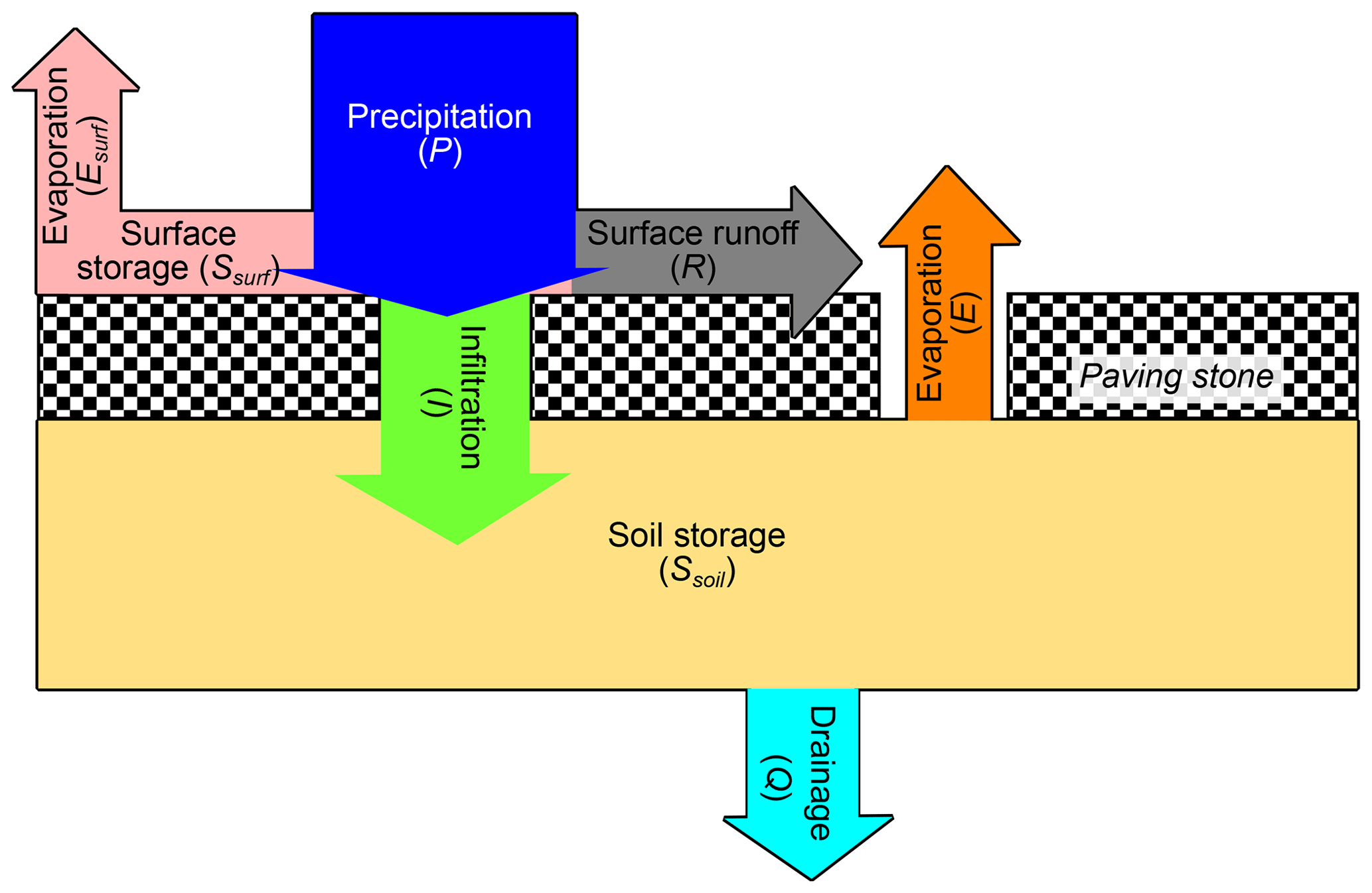
The flux and state variables considered within FluSM are depicted in Fig. 1 and explained in the following. At the ground surface, precipitation (P) first fills the surface storage, which has a defined capacity (C_surf). We defined the C_surf as the water storage capacity that exists at the atmosphere–pavement boundary. Following Mansell and Rollet (2009), it consists of a depression storage (storage due to the micro-relief of the surface) and the wetting capacity of the surface (amount of water required for wetting the surface). Water is removed from the surface storage during subsequent dry periods by surface evaporation (E_surf). The fluxes E_surf and P determine the state of the surface storage (S_surf). Excess P splits into surface runoff (R) and infiltration (I) depending on the infiltration rate (I_cap). Within the soil, the infiltrating water fills the soil storage, which is emptied by the processes of evapotranspiration (E) and vertical drainage (Q). Hence, the state of the soil storage (S_soil) is controlled by the fluxes I, E, and Q.

Figure 1 Flux and state variables defined within FluSM.

FluSM involves four different computational steps and requires time series of volumetric soil moisture (θ), potential evaporation (E₀) and P as inputs, as well as a plot-specific I_cap (Fig. 2). For the application of FluSM, there are some requirements concerning the input data and the soil hydrological behavior of the site. These requirements are briefly listed in the following:

• θ should be measured close to the ground surface,

• θ time series should be corrected for fluctuations not related to water fluxes (e.g., due to temperature effects),

• there should be free vertical drainage.

Figure 2 Inputs and computational steps of FluSM.

The computational steps work with an hourly resolution, except the surface water balance, which is calculated with a 10 min temporal resolution and aggregated to an hourly resolution at the end. In step 1 of FluSM, C_surf is determined from time series of P and θ. Therefore, first the amplitude of the soil moisture response is calculated for each rain event. Afterwards, the events are grouped according to precipitation sums and the median soil moisture response is calculated for each precipitation class. For classes below a specified response threshold, we assume that rainfall did not exceed C_surf. Based on this assumption, C_surf is defined to be equal to the precipitation sum of the highest class not exceeding the response threshold (illustrated in Fig. 3). Consequently, C_surf integrates the depth of water stored at the ground surface but also the depth of water stored within the soil above the soil moisture sensor.

In step 2, the surface water balance is calculated as follows:

$$\begin{array}{}\text{(1)}& P\left(t\right)={\displaystyle \frac{\mathrm{d}{S}_{\mathrm{surf}}}{\mathrm{d}t}}+I\left(t\right)+R\left(t\right).\end{array}$$

While S_surf is below C_surf, rainfall only fills the surface storage (step 2a of FluSM). During subsequent dry periods, the surface storage is emptied by E_surf with rates specified by the E₀. Thereby, we assume that E_surf can be neglected during times of rainfall and further that there is no condensation of water vapor on the ground surface (times with negative E₀). In steps 2b and 2c, the excess of P divides into I (Eq. 2) and R (Eq. 3) and the partitioning between the fluxes is controlled by a plot-specific I_cap, which is constant over time.

$$\begin{array}{}\text{(2)}& {\displaystyle }I\left(t\right)=\left\{\begin{array}{ll}P(t& \text{if}P\left(t\right)\le I_{\mathrm{cap}}\\ I_{\mathrm{cap}}& \text{if}P\left(t\right)>I_{\mathrm{cap}}\end{array}\right.\text{(3)}& {\displaystyle }R\left(t\right)=\left\{\begin{array}{ll}\mathrm{0}& \text{if}P\left(t\right)\le I_{\mathrm{cap}}\\ P\left(t\right)-I_{\mathrm{cap}}& \text{if}P\left(t\right)>I_{\mathrm{cap}}\end{array}\right.\end{array}$$

After calculating the surface water balance, the soil water balance is calculated in step 3 (Eq. 4).

$$\begin{array}{}\text{(4)}& {\displaystyle \frac{\mathrm{d}{S}_{\mathrm{soil}}}{\mathrm{d}t}}=I\left(t\right)-E\left(t\right)-Q\left(t\right)\end{array}$$

We use the measured change of the soil moisture (d$\mathit{\theta }/\mathrm{d}t$) as a proxy for d$S_{\mathrm{soil}}/\mathrm{d}t$ (note that d$\mathit{\theta }/\mathrm{d}t$ is negative for times with decreasing θ, while it is positive for times with increasing θ). By substituting d$S_{\mathrm{soil}}/\mathrm{d}t$ with d$\mathit{\theta }/\mathrm{d}t$ in Eq. (4), soil water fluxes (mm/h) are converted to soil moisture fluxes (vol %/h). Since measured d$\mathit{\theta }/\mathrm{d}t$ integrates all soil moisture fluxes, the individual fluxes cannot be inferred directly from the measurements. We therefore describe Q as a function of θ by using an unit gradient approach (Hillel, 1998) with the Burdine–Brooks–Corey parametrization of the unsaturated hydraulic conductivity (Brooks and Corey, 1964) (Eq. 5, hereinafter called drainage model).

$$\begin{array}{}\text{(5)}& Q=k_{\mathrm{s}}\cdot {\left({\displaystyle \frac{\mathit{\theta }-{\mathit{\theta }}_{\mathrm{r}}}{{\mathit{\theta }}_{\mathrm{s}}-{\mathit{\theta }}_{\mathrm{r}}}}\right)}^{\frac{\mathrm{2}+\mathrm{3}B}{B}}\end{array}$$

Where k_s is the saturated hydraulic conductivity, θ_r the residual water content, θ_s the saturated water content and B the pore size distribution index. While θ is the only variable controlling Q, E is also controlled by E₀. For dry periods with an atmospheric demand below a specified threshold, we assume evaporation to be negligible and thus $-\mathrm{d}\mathit{\theta }/\mathrm{d}t$ to be equal to Q. Therefore, we can use the soil moisture observations of these periods to fit the drainage model (Eq. 5) and to derive the parameters k_s and B and their associated standard errors (σ_ks and σ_B). In FluSM, the least-square optimization algorithm implemented in the Python module SciPy is used for the fitting procedure. Thereby, θ_r and θ_s are obtained from the minima and the maxima of the soil moisture time series.

In the next step, the calibrated drainage model is used to predict Q from the measured soil moisture time series (FluSM step 3b). Assuming that I and E do not occur simultaneously, we obtain I and E by closing the mass balance (Eqs. 6 and 7).

$$\begin{array}{}\text{(6)}& {\displaystyle }I\left(t\right)=Q\left(t\right)+{\displaystyle \frac{\mathrm{d}\mathit{\theta }}{\mathrm{d}t}}\text{if}-{\displaystyle \frac{\mathrm{d}\mathit{\theta }}{\mathrm{d}t}}<Q\left(t\right)\text{(7)}& {\displaystyle }E\left(t\right)=-{\displaystyle \frac{\mathrm{d}\mathit{\theta }}{\mathrm{d}t}}-Q\left(t\right)\text{if}-{\displaystyle \frac{\mathrm{d}\mathit{\theta }}{\mathrm{d}t}}>Q\left(t\right)\end{array}$$

We use two constraints to close the soil water balance, which are (1) no evaporation while water is available in the surface storage and (2) no influx into the soil storage during dry periods (see Sect. 4 for an explanation and discussion of the constraints). For times where one constraint is active, Q is assessed directly from the observed $-\mathrm{d}\mathit{\theta }/\mathrm{d}t$, while at the same time either E (constraint 1) or I (constraint 2) is set to 0.

Finally, the soil water balance and the surface water balance are linked by mapping infiltration calculated by the soil water balance on infiltration calculated by the surface water balance. In this step, a monthly variable scaling factor is determined from the slope of a linear regression, which is performed between the cumulative infiltration obtained from the soil water balance and cumulative infiltration of the surface water balance. This scaling factors represents the depth of the soil bucket (mm), which is needed to infer S_soil (mm) from θ (vol %). After determining the scaling factor, it is applied to transform all soil moisture fluxes into water fluxes.

2.2 Case study

For our case study, we used the data set provided by Schaffitel et al. (2020), which includes temperature-corrected soil moisture times series, infiltrometer measurements and climate data, recorded underneath PPs within the city of Freiburg (Germany). At each PP included within the data set, soil moisture was measured in various depths over a 2-year lasting study period (November 2016–October 2018). Using the soil moisture measurements, Schaffitel et al. (2020) classified the PPs into free-draining PPs and such with a restricted drainage behavior. This classification was based on a combination of statistical analysis and visual inspection. Plots were classified as “restricted drainage” when soil moisture reached saturation frequently during rain events and remained saturated even after the end of rainfall. In contrast, plots which showed a fast recession of soil moisture were classified as “free drainage”, since the fast recession indicates a high hydraulic conductivity of underlying soil layers. For our case study, we only included the 15 free-draining PPs (hereinafter called plots), since this is a basic requirement for using FluSM.

According to the local construction authority, the PPs of the case study should not have a porous reservoir layer. Coarse gravel that could serve as kind of porous reservoir layer was only encountered at two plots located on a private parking lot (CP12 and CP2). Hydraulic conductivity measurements were performed neither during construction works nor successively. It was therefore planned to extract undisturbed soil samples for determining the hydraulic conductivity function from multistep outflow experiments in the laboratory. Due to the high fraction of soil skeleton and due to the high soil compaction it was impossible to extract undisturbed soil samples.

Schaffitel et al. (2020) used the data of the infiltration experiments to derive plot-specific values for I_cap, as well as initial and end infiltration rates (I_start and I_end). Thereby, infiltration experiments were performed only once at the beginning of the study period. Due to the lack of successive infiltration experiments, a direct quantification of the clogging progress over the study period is not possible. However, recorded soil moisture dynamics should allow for an indirect assessment of clogging dynamics. In this way, Razzaghmanesh and Borst (2018) used soil moisture measurements to study the clogging progress on a PP over time. For the PPs of our study, we visually analyzed the measured soil moisture dynamics over the study period. Since we did not observe a change in the dynamics over time, we expect that the state of surface clogging remained more or less constant over the study period. A possible explanation for the surface clogging remaining more or less constant over the study period might be that none of the PPs were newly built, and thus all plots were already clogged at the beginning of the study period.

Table 1 shows the properties and parameters of the 15 PPs included within this case study.

Table 1 Characteristics of the PPs considered within the case study. For further information, see Schaffitel et al. (2020).

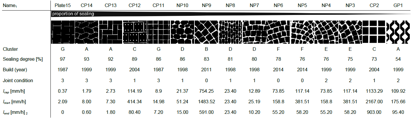
¹ The names include the type of PPs (plate; CP: concrete paver; NP: natural paver and GP: grass paver) and a number assigned in descending order according to the degree of surface sealing. ² Assessed from the A parameter of the fitted Philip infiltration model (Schaffitel et al., 2020), which represents the theoretical minimum of the infiltration rate.

For the city of Freiburg (Germany), data of four different climate stations are available (Schaffitel et al., 2020). For our case study (Sect. 3.1 and 3.2), we used the meteorological data of the WBI (Weinbauinstitut Freiburg) climate station, since this station is effected by the urban climate and data are free from gaps. Over the 2-year study period, a total of 2440 mm of rainfall was recorded, while potential evaporation sums up to a total of 1570 mm. In order to estimate the uncertainty of the climate input data, we used data of all four climate stations (Sect. 3.3). Thereby, data of two climate stations exhibit data gaps, while the other two are free from data gaps. In order to obtain continuous time series for all four stations, data gaps were filled with the associated records of the WBI climate station. For our case study, the threshold for the soil moisture response (required for FluSM step 1) was set to 0.4 vol %, which represents 4 times the resolution of the soil moisture sensors. Regarding the threshold for potential evaporation (required for FluSM step 2a), we used a value of 0.5 mm/d, which represents a compromise between a low evaporative demand and high number of observations for fitting the drainage model.

2.3 Uncertainty analysis for the case study

Errors in hydrological modeling may arise from four different sources, which are (a) uncertain parameters, (b) uncertain input variables, (c) uncertainties in model structure and (d) selection of data used for calibration (Deletic et al., 2012). For our case study, we developed an approach to quantify the effect of parameter and input uncertainty on the results of FluSM. In the process, we first estimated uncertainties for each parameter and input variable and then propagated these through FluSM by means of 10 000 Monte Carlo simulations generating the uncertainty range for each component of the water balance.

Uncertainties in the input variables (θ,P and E₀) may arise from systematic and from random errors. For the climatic input variables, only systematic errors were considered. Such errors may arise from (a) the heterogeneity of the urban climatic conditions and (b) offsets in measurements. On the scale of an urban canyon, Koelbing et al. (2017) showed that the effect of (a) on E₀ is mainly caused by the spatiotemporal variability of shading. Following Bitar (2004), we considered this uncertainty by a factor ranging between 0.5 and 1.4, which during the Monte Carlo simulations was randomly resampled from a uniform distribution. Due to the large range considered, the analysis should also account for uncertainties in estimating E₀. For rainfall, a certain degree of the spatial heterogeneity is captured by the variability among the four climate stations within the study area. We accounted for this variability by using the four P time series as ensembles for the Monte Carlo simulations. Additionally, we multiplied the rainfall time series by a factor ranging between 0.8 and 1.2 (uniform distribution) to account for measurement bias and small-scale rainfall variability (e.g., within an urban canyon). Regarding the soil moisture measurements, systematic errors are irrelevant since all calculations are based on the relative change of θ over time rather than on absolute θ. Due to the temperature correction schemes applied by Schaffitel et al. (2020), we expect that random errors were removed to a great extent. Therefore, errors of soil moisture were not considered within the uncertainty analysis.

Uncertainties also exist for the parameter I_cap and the two parameters of the drainage model (k_s and B). For I_cap, we specified these uncertainties to range between the plot-specific I_start and I_end (Table 1). Parameter uncertainty of k_s and B was assessed by their standard errors (σ_ks and σ_B) obtained during the fitting procedure. Within the Monte Carlo framework, we used uniform random resampling for all parameters.

3 Results

3.1 Processes in the FluSM approach

First, we derived the plot-specific C_surf. For our data set, the uppermost sensor was located directly beneath the paving layer. Hence, C_surf comprises the amount of water stored at ground surface (depression storage and wetting capacity) and the amount of water stored within the joint material. Figure 3 shows the classes of median soil moisture responses and reveals a C_surf of 2.5 mm for plot CP14 (see Appendix A for the C_surf of the other plots of the case study). The filling and emptying of the surface storage over three wet–dry cycles is depicted in Fig. 4.

Figure 3 Determination of C_surf for plot CP14 (FluSM step 1).

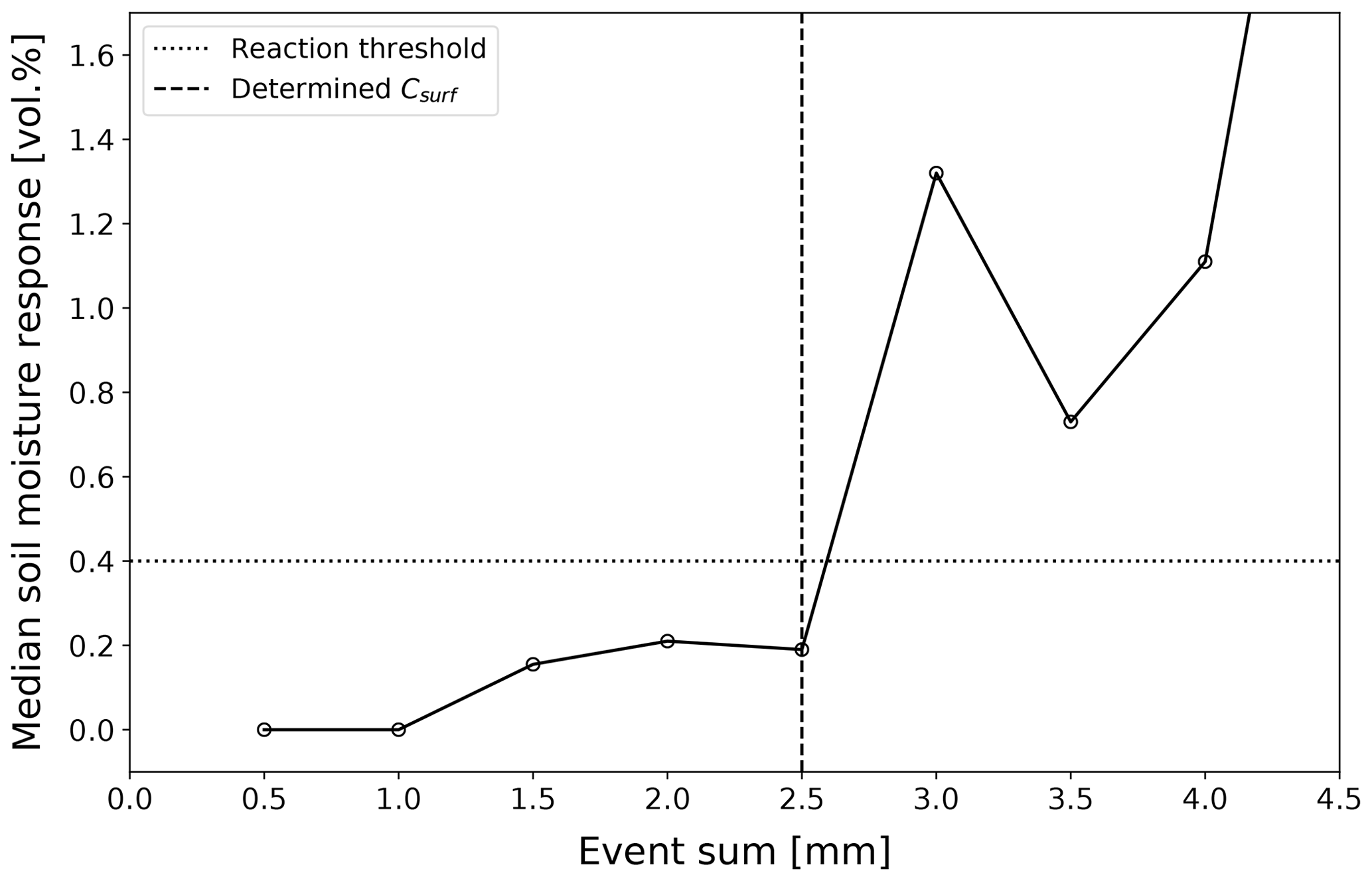
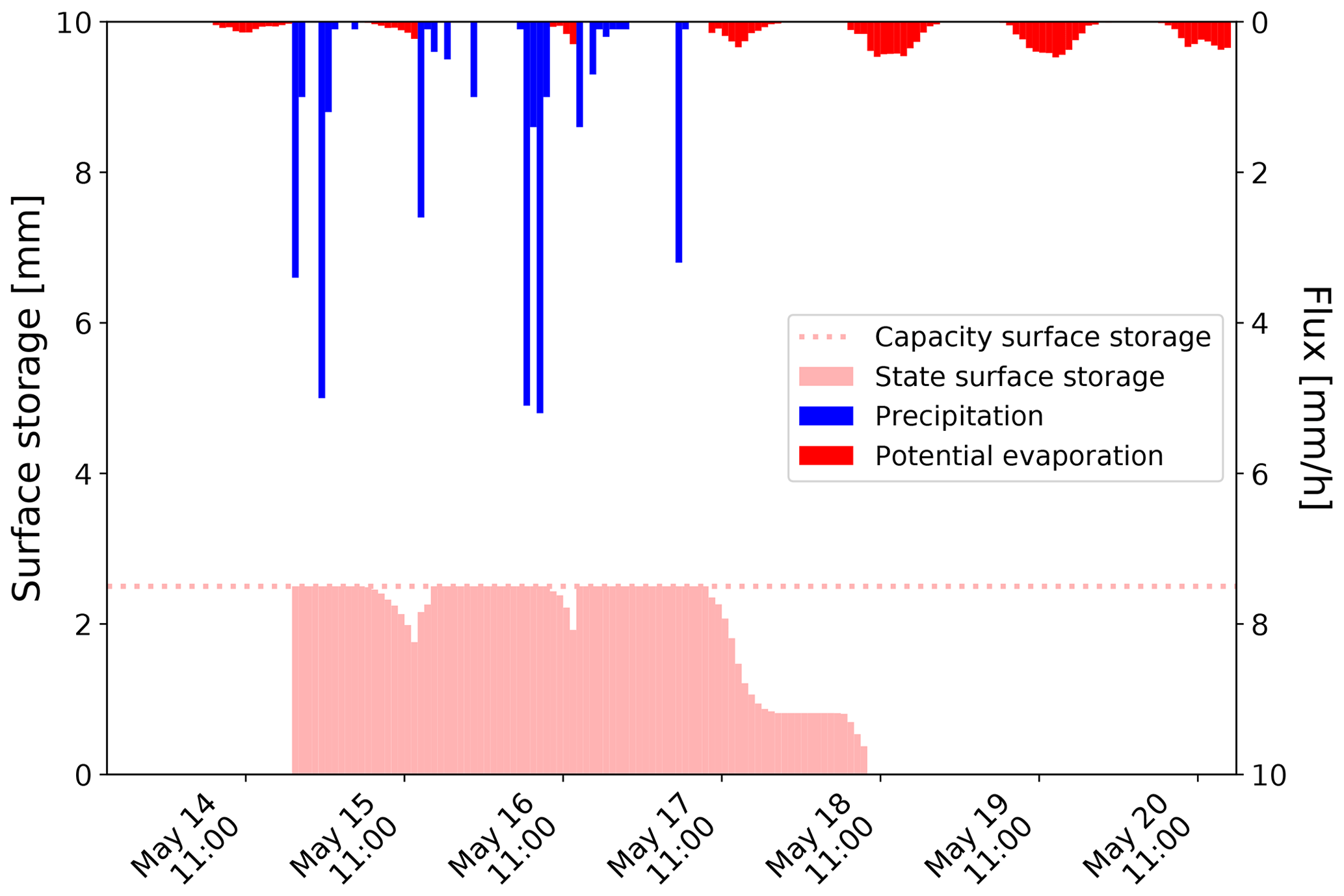
Figure 4 Filling and emptying of the surface storage over three separated wet–dry cycles in May 2018 at plot CP14 (FluSM step 2a).

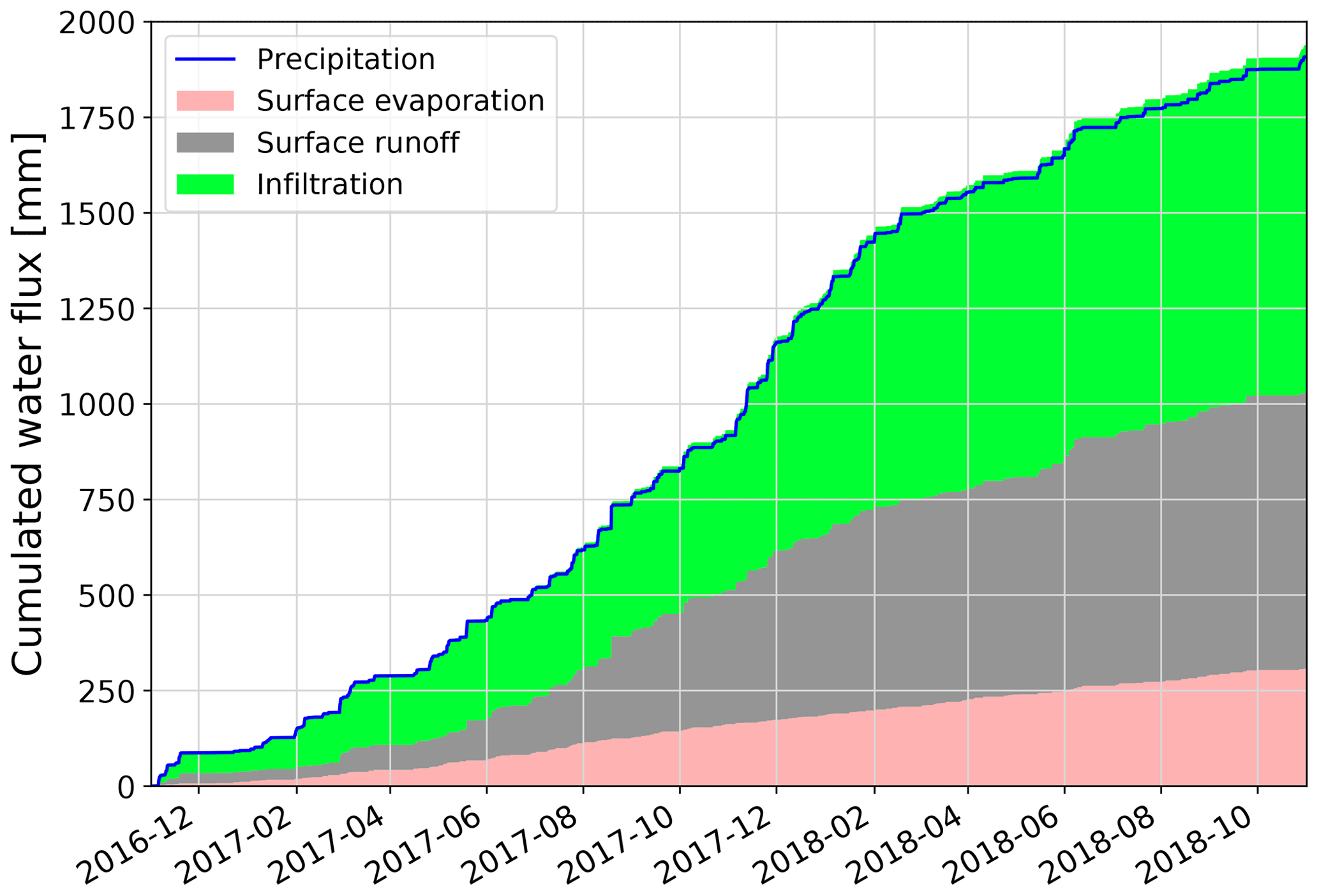
During each event depicted in Fig. 4, the surface storage was entirely filled, while it was at least partially emptied during subsequent dry periods. When the surface storage is entirely filled, the parameter I_cap determines the partitioning of excess P into infiltration and surface runoff. For plot CP14, I_cap is quite low with 1.79 mm/h, but rainfall intensities measured at the WBI climate exceed 2 mm/h for only around 27 % the time with observed rainfall. Although the formation of surface runoff is rare, its quantity is still considerable at this plot. Figure 5 shows the derived surface water balance for plot CP14, with around 40 % of precipitation input leading to surface runoff (approx. 720 mm over the study period). Infiltration still dominates the surface water balance with around 830 mm. Surface evaporation accounts for around 290 mm (16 % of the precipitation input).

Figure 5 Cumulative surface water balance of plot CP14 over the entire study period.

For the soil water balance, first the parameters of the drainage model (Eq. 5) were determined by fitting of the drainage model to soil moisture observations made during periods with a low potential evaporation (Fig. 6).

Figure 6 Fitting of the drainage model for plot CP14. The inset shows the frequency distributions of all soil moisture observations and the observations used for fitting of the drainage model.

The parameters obtained for plot CP14 account for 1.44 ± 0.05 vol % for k_s and 1.78 ± 0.1 for B. The root-mean-square error of the fit is 0.04 vol %/h, which indicates a good quality of the fit. This is also reflected in the narrow confidence intervals depicted in Fig. 6. Additionally, the inset of Fig. 6 shows the density of the observations used for fitting (right side) and the entire population of all observations (left side). Although the distributions differ, the observations used for fitting cover the range of the entire population to a large extent. Results for the other plots are reported in Table A1 of Appendix A.

In the next step of applying the soil water balance, the fitted drainage model was used to predict drainage rates from the measured soil moisture time series (FluSM step 3b). By using predicted drainage rates and the observed change of soil moisture, the soil water balance was closed. This is exemplarily shown in Fig. 7 for a period of 30 h for plot CP14. Thereby, the effect of the model constraints become visible as surface evaporation starts only after the surface storage is completely empty and no water is infiltrating after the end of the rainfall event. The entire soil water balance of plot CP14 is shown in Fig. 8. For this plot, evaporation accounts for around 10 % of the infiltrating water, while drainage dominates with 90 %.

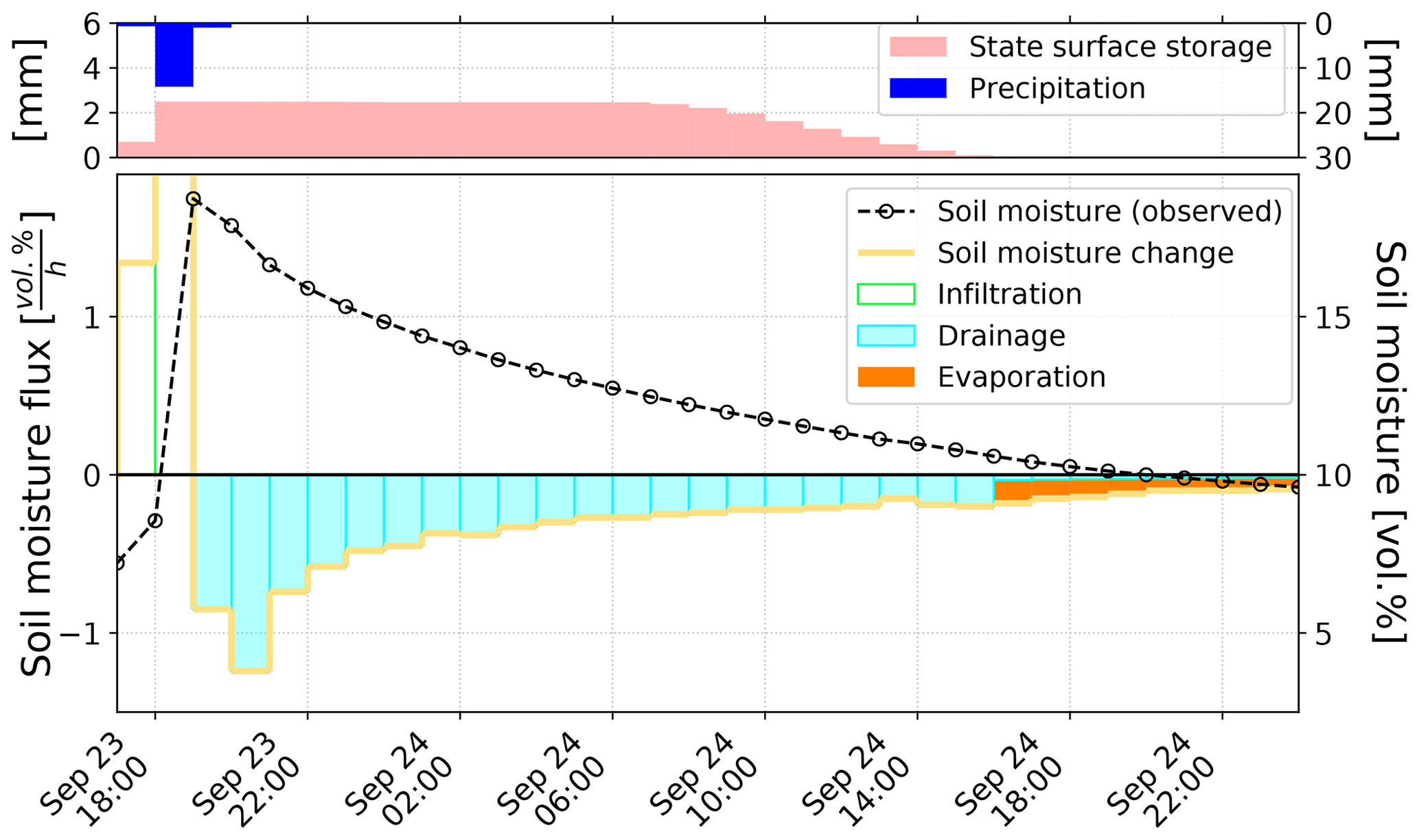
Figure 7 Closure of the soil water balance from measured d$\mathit{\theta }/\mathrm{d}t$ and predicted drainage loss for plot CP14 over a period of 30 h.

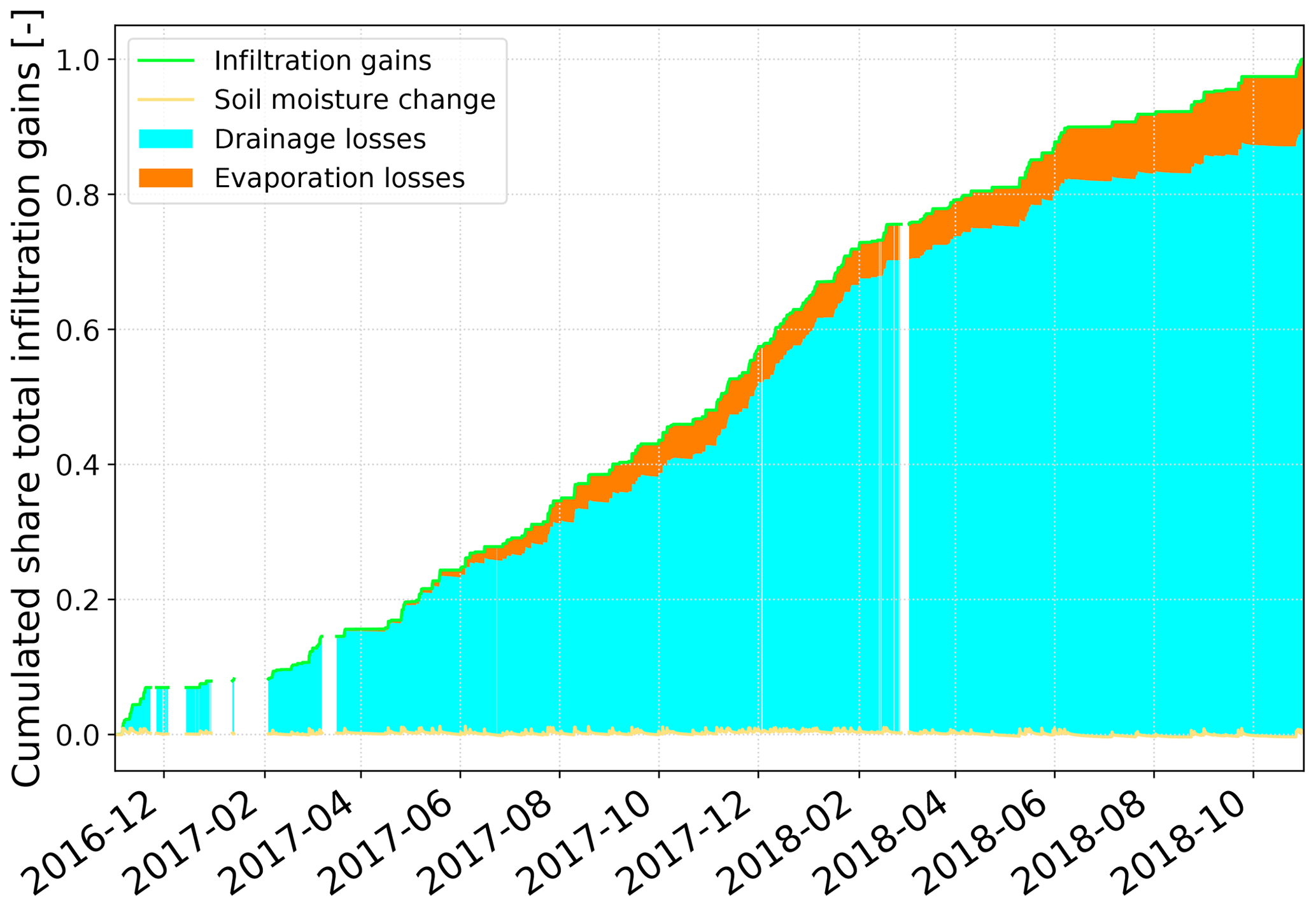
Figure 8 Soil water balance for plot CP14. Gaps in the soil water balance are due to gaps in the recorded soil moisture time series.

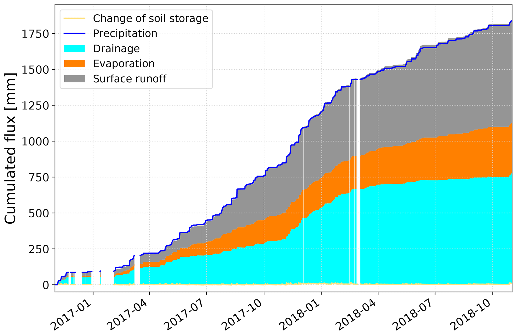
In FluSM step 4, the depth of the soil bucket (mm) is derived on a monthly time basis. For plot CP14, the median of the monthly variable bucket depths accounts for 60 mm, with a standard deviation of 28 mm. Values for the other plots of the case study are provided in Appendix A. Applying the bucket depths on the soil water balance, the entire water balance was obtained (Fig. 9). The transformation of soil moisture fluxes into water fluxes leads to minor deviations between the total precipitation input and the summarized water fluxes. For plot CP14, these deviations are negligible since they account for less than 0.3 % of the total water balance. While the surface water balance of plot CP14 revealed a total infiltration of 830 mm (Fig. 5), the complete water balance shows that most of this infiltration leads to drainage, which forms the largest part of the water balance (770 mm). Furthermore, the water balance shows a total evaporation of 350 mm, which is approx. 19 % of the precipitation input.

Figure 9 Cumulated water fluxes of the entire water balance for plot CP14.

3.2 Benchmarking of FluSM for the case study

Validating the fluxes calculated for the PPs of the case study is challenging, since we did not measure the fluxes directly. To overcome this problem, we conducted a literature review on long-term water fluxes reported for PPs and compared them with our results. Since the water balance of PPs is controlled by various factors and since these factors vary between the different studies, this comparison can serve only as rough validation. Foremost amongst the factors which control the water balance of PPs are local microclimatic conditions, soil properties, water availability and surface properties.

Studies on the long-term water balance of PPs under realistic field conditions are scarce. Known studies include lysimeter measurements (Flöter, 2006; Rim, 2011; Timm, 2019; Wessolek and Facklam, 1997), drainage measurements (Brown and Borst, 2015), and combined soil moisture and drainage measurements (Ragab et al., 2003). A recent review by Timm et al. (2018) further includes results of non-published studies. However, none of these studies includes more than six different PPs, and plot-specific parameters (e.g., degree of surface sealing, infiltration rate, surface clogging) are poorly documented. Given the differences in the climatic conditions among the studies, it is hardly feasible to make a general statement on the long-term water balance of PPs within the urban environment. In addition, Illgen (2009) showed that infiltration rates measured at same type PPs can range over at least 1 order of magnitude. Table 2 shows the results found in literature on the long-term water balance of PPs.

Table 2 Values reported in literature for the long-term water balance of PPs. NA – not available

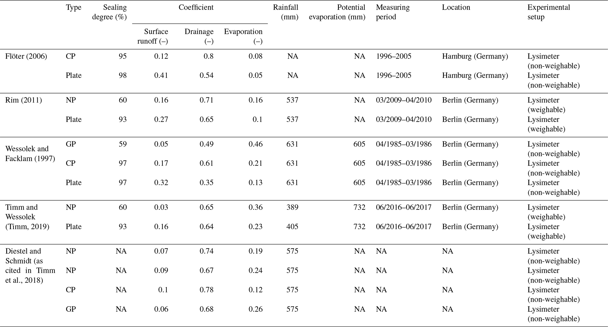
Table 3 shows the summarized water fluxes for all plots in our case study. Note that times with data gaps in soil moisture data were excluded from FluSM calculations, resulting in lower rainfall amounts. In agreement with all other available studies (Table 2), the results of our case study show that the drainage flux dominates the water balance for all PPs except for plot CP15. For PPs with an I_cap above 9 mm/h, surface runoff coefficients were below 10 %, while PPs with I_cap values above approx. 70 mm/h showed negligible surface runoff (below 12 mm). Only at plots with I_cap below 3 mm/h (CP15, CP14 and CP13) is surface runoff a major component of the water balance, accounting for 30 %–80 % of precipitation.

Table 3 Summarized fluxes over the entire measuring period for all plots (evaporation includes E and E_surf).

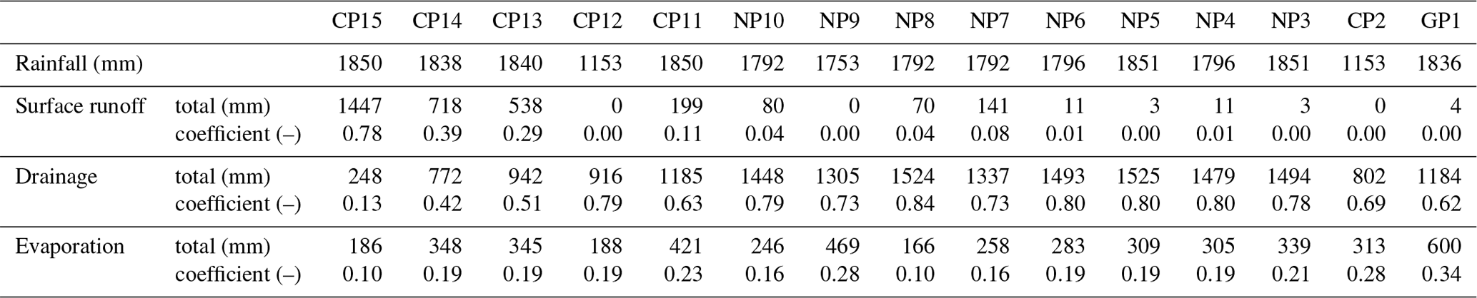
Figure 10 Range of long-term water fluxes reported in the literature for different PP types compared with the results of our case study.

In Fig. 10, our results are compared to the long-term water balance reported in the literature for different types of PPs. For plates, the four studies found in the literature show a lower runoff and a higher drainage coefficient compared to the plate included in our case study. This is due to the low infiltration rate measured at our plate (0.37 mm/h), which lies around 10 times below the rates measured by Wessolek and Facklam (1997) for their plate lysimeter. For concrete paving stones, patterns of our results are comparable with literature values, although our results show a larger variation for this group. This is mainly due to the large range of infiltration rates that we measured for this group (ranging from 1.79 to 1133 mm/h). Nevertheless, the results consistently show that drainage dominates the water balance for all concrete pavers. In addition, for natural pavers our results and the literature values show equal patterns, with drainage dominating the water balance, followed by evaporation, while surface runoff accounts for the smallest part of the water balance. Compared to literature values, we predicted slightly higher drainage and at the same time smaller runoff and evaporation. For grass pavers, our results for drainage and evaporation lie within the range of the literature values.

In general, our results are consistent with the patterns found by previous studies. Due to the small number of studies on long-term water fluxes of PPs and the different environmental conditions involved, a direct validation of the FluSM results is difficult. Such a direct validation would only be possible for sites where water fluxes and θ were measured simultaneously.

3.3 Uncertainty analysis

We performed 10 000 Monte Carlo simulations with FluSM in order to quantify the effect of uncertain inputs and parameters on the results of the case study. Based on our assumption of input uncertainty, precipitation ranged between 550 and 1150 mm/yr, while potential evaporation ranged between 400 and 1150 mm/yr (Fig. 11b). Hence, we considered a wide range of climatic inputs, which should cover the variability of urban microclimatic conditions and further account for measurement errors. From the Monte Carlo simulations, we obtained distributions for each water balance coefficient (Fig. 11a). In the following, we define uncertainty ranges as the distance between the 5th and 95th percentile of the distributions.

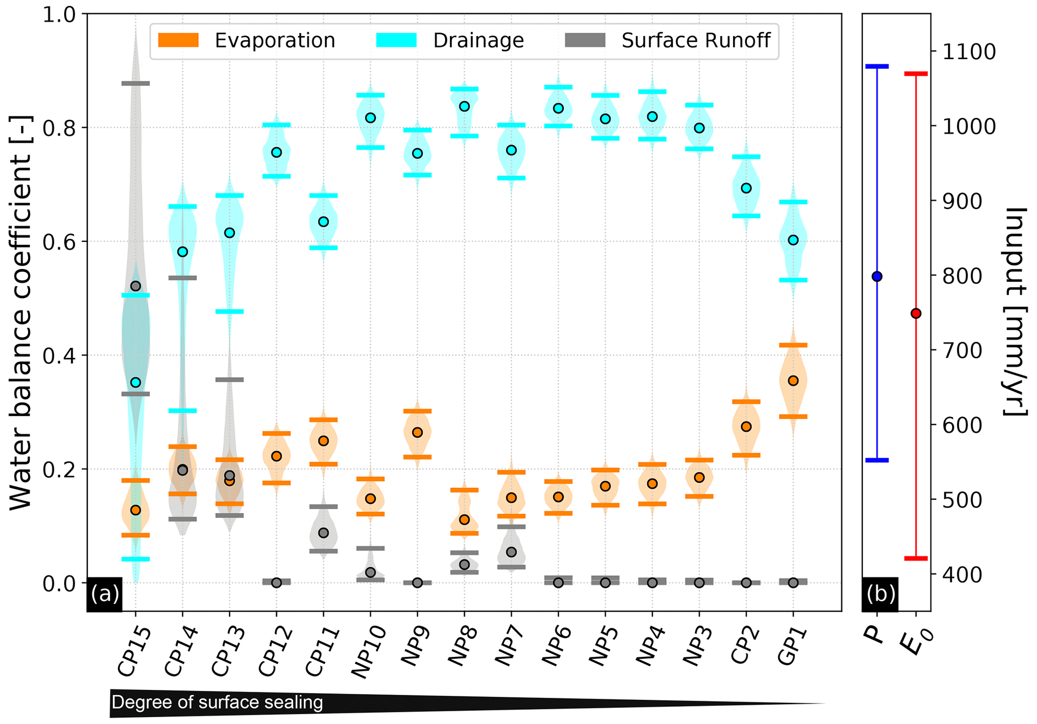
Figure 11 Violin plots of water balance coefficients obtained from the 10 000 Monte Carlo simulations (a) and the range of the considered variability of the climatic input (b). Points indicate the median of all runs, while horizontal lines represent the 5th and 95th percentiles of the distributions.

Even when considering uncertain inputs and parameters, the aforementioned patterns of drainage forming the largest water balance component at almost all PPs, evaporation accounting for at least 10 % of the water balance and surface runoff being negligible for PPs with an average infiltration rate above 70 mm/h remain unchanged. Uncertainty ranges for evaporation coefficients account for ±6 % of the total water balance and are similar for all PPs. Since predicted uncertainties for evaporation are small, the considered input and parameter uncertainties have only a small effect on this water balance component. In contrast, uncertainties in surface runoff and drainage coefficients differ among the individual plots. These differences can be attributed to the parameter uncertainty of the infiltration rate, which we defined as ranging between the plot-specific initial and end infiltration rate. While the results are very robust for plots with high infiltration rates (e.g., NP4, NP3, CP2 and GP1), there are large uncertainties for PPs with low infiltration rates (e.g., CP15, CP14 and CP13). For PPs with an infiltration rate above 70 mm/h, the uncertainty of this parameter has no effect on the water balance, since surface runoff is negligible even when end infiltration rates are used for FluSM.

4 Discussion

In the following, we first discuss the benefit of the FluSM approach and point out possible fields of application in regard to requirements of the approach. Afterwards, model assumptions and concepts are discussed. Finally, we focus on urban hydrological issues related to our case study on the water balance of PPs.

The FluSM approach allows for deriving continuous water fluxes from soil moisture and meteorological measurements. Compared to direct measurements of soil hydrological fluxes, this poses a relatively easy and cheap method for water balance studies and is especially valuable for fields with limited soil hydrologic knowledge (e.g., missing soil hydrologic parameters or lack of knowledge on the correct representation of processes). In this way, we successfully applied FluSM to derive long-term, high-resolution hydrological fluxes for 15 different PPs under field conditions. So far, such data were obtained only by costly lysimeter studies. Besides the application for water balance studies, FluSM may also be beneficial for studying soil hydrological processes and contribute to an increased data availability. In the future, data-driven derivations of soil hydrological fluxes might serve as a simulation benchmark for the application of process-based hydrological models. Regarding the ever-increasing availability of soil moisture data on different spatial scales, the demand for such parsimonious approaches should increase.

For an application of FluSM, we recommend preprocessing soil moisture time series in order to correct for fluctuations not related to water fluxes. Such fluctuations may, e.g., originate from the temperature dependency of soil moisture measurements (Kapilaratne and Lu, 2017; Qu et al., 2013; Wraith and Or, 1999). An efficient correction method has been presented by Schaffitel et al. (2020).

An intrinsic assumption of the applied unit gradient approach is that drainage occurs freely (no impeding layers) with gravity-driven rates (minor influence of matrix potential). This concept is widely used in bucket-type water balance models for describing drainage (e.g., Albertson and Kiely, 2001; Famiglietti and Wood, 1994; Rodriguez-Iturbe et al., 1999). Furthermore, FluSM requires a high plot-specific infiltration rate. This parsimonious approach allows applying FluSM for locations where it is difficult to estimate suction heads or matrix potentials. We recommend to determine the infiltration rate from plot-specific infiltration experiments, since a correct estimation is crucial for the results. Since FluSM is a data-driven approach that requires plot-specific soil moisture measurements, infiltration experiments could be performed together with the installation of soil moisture sensors.

The requirements for an application of FluSM should be fulfilled for PPs, since constructional regulations require a high infiltration rate and a high hydraulic conductivity for all PP layers (Borgwardt, 2001; FGSV, 2012). Besides the application on PPs, FluSM is also applicable for bare soils in case its requirements are met. Furthermore, FluSM should also be applicable for sites with vegetation cover, since soil moisture measurements should capture the effect of root water uptake. However, for plots with vegetation cover, the location of soil moisture sensors within the profile should be adapted. While the effect of soil evaporation should be most evident in shallow depths, root water uptake may also act on deeper depths. Therefore, the installation of multiple sensors covering the entire rooting depth should be considered. However, for fields with seasonally varying canopy coverage (e.g., deciduous forests) and sites with seasonally variable vegetation cover (e.g., agricultural fields), an adaption of the FluSM routine may be necessary in regard to the surface storage. Currently, the implementation assumes that the surface storage capacity remains constant over time. This is a reasonable assumption for PPs and should also be valid for, e.g., bare soil and grassland sites. For our case study, we obtained a surface storage capacity between 1 and 4.5 mm, which is in accordance with the range specified by previous studies (e.g., Brown and Borst, 2015; Flöter, 2006; Illgen, 2009; Starke et al., 2010; Wessolek et al., 2008; Wessolek and Facklam, 1997; Wiles and Sharp, 2008). However, for sites with seasonally varying vegetation or canopy cover the concept of a constant surface storage capacity might be problematic (Link et al., 2004). Under such conditions, an adaption of the routine should be considered. We think that a seasonally variable surface storage capacity might be determined directly from soil moisture and precipitation data by adapting the determination (FluSM step 1) to work on a monthly basis. This would require measurements over multiple years. Further alternatives to account for a seasonally variable surface storage capacity include using throughfall measurements or augmenting FluSM by a canopy interception model.

For most soils, the infiltration rate decreases during the infiltration course, which is mainly due to declining matrix suction gradients during the proceeding of the infiltration front (Hillel, 1998). In FluSM, infiltration is represented by a constant rate, potentially leading to an error in the calculated infiltration and surface runoff fluxes. Besides matrix flux, infiltration may also be controlled by further processes (e.g., preferential flow and hydrophobicity). Such may be the case for PPs. For the plots of our case study, the possible variability of the infiltration rate over time is documented in data of the infiltration experiments under ponded conditions, which were used to derive plot-specific initial and end infiltration rates (Schaffitel et al., 2020). Thereby, the range between initial and end infiltration rates should capture the variability between dry and wet soil conditions and reflect the possible variability caused by the temporal distribution of storm and inter-storm periods. We considered this range in our uncertainty analysis. The error caused by the usage of a constant infiltration capacity is reflected in the uncertainty ranges obtained for surface runoff (Fig. 11). Our results show that this error is only relevant for three plots with a very low infiltration rate, while it is small for the majority of the plots and becomes negligible for plots with an infiltration rate above 70 mm/h. Hence, the results for plots with a high infiltration rate are not affected by the concept of using a constant infiltration rate, while the results for plots with an infiltration rate below 9 mm/h should be regarded with care. This highlights the requirement of a high plot-specific infiltration rate for the reliability of the FluSM approach.

Within FluSM, the parameters of the drainage model are derived by fitting. Therefore, the soil water balance relies on the quality of the fit. In order to obtain reliable fits, the number of observations should be high. Therefore, soil moisture measurements should cover at least an entire year, including at least one season with low atmospheric demand.

Horizontal subsurface may occur at boarders between soil layers in case of declining soil hydraulic conductivity. So far, horizontal subsurface flow is not considered in FluSM. Within a PP system (pavement, bedding, base and subbase layer), horizontal subsurface flow should only play a minor role, since a high hydraulic conductivity is required for all layers. This is also reflected in the free drainage behavior observed for the PPs of our case study. However, horizontal subsurface flow may occur at the bottom of the PP system (e.g., at the border between subbase layer and underlying soil). Such horizontal subsurface flow would not affect the calibration of the drainage model, since it is not it is not relevant whether the soil moisture recession is due to vertical drainage or if it is due to horizontal subsurface flow. Both fluxes are summarized in the calculated drainage flux. The calibration of FluSM would be problematic only for plots showing a restricted drainage behavior, which we therefore excluded from our case study. In cases where horizontal subsurface flow at the bottom of the PP system is of interest, an extension of FluSM is possible. In a parsimonious approach, the saturated hydraulic conductivity of the underlying soil layer could be used as single parameter to describe the partitioning between deep percolation and horizontal subsurface flow at this border.

Within FluSM, we use a regression approach to derive the bucket depth from the observed soil moisture reaction and from the infiltration calculated by the surface water balance. Therefore, FluSM does not rely on an assumed bucket depth, which poses a major advantage over other bucket-type water balance models, which were shown to be very sensitive on the assumed soil (bucket) depth (Boulet et al., 2000; Breña Naranjo et al., 2011). Furthermore, the bucket depth in FluSM is variable on a monthly timescale, which enables to account for processes variable over time (e.g., rooting depth, temperature dependency of water fluxes, evaporation depth). Due to the derivation of the bucket depth by a regression approach, all site-specific characteristics are lumped into this parameter, hampering a physical interpretation. This gets obvious when comparing the calculated bucket depth, e.g., for the plots CP2 and GP1 of our case study (Table 4). On both plots, surface runoff is negligible (both plots have a very high infiltration rate) and therefore, the amount of total infiltration should be comparable (although not identical, e.g., due to different surface storage capacities). Hence, the deviations between the derived bucket depths for those plots originate from differences in the amplitude of the soil moisture reaction to infiltration. This may be caused by differences in the three-dimensional propagation of the wetting front underneath the joints (e.g., caused by spatial distribution of impermeable paving stones and joints or by differences in soil properties), soil-specific parameters (e.g., the amount of skeleton) and by the connection of soil moisture sensors to surrounding soils.

Our case study on the water balance of PPs is located in the field of urban hydrology. A key characteristic of urban hydrology is the fast concentration, collection and conveyance of surface runoff (Shuster et al., 2005). This causes a high flashiness in surface flow hydrographs, and modeling calls for a high temporal resolution of rainfall data. Besides the temporal resolution, the spatial resolution of rainfall is also decisive, since urban hydrological processes are characterized by a high variability not only in time but also in space (Cristiano et al., 2017). Since high-resolution rainfall data are rarely available, precipitation is often seen as a main source of uncertainty in urban hydrology (Cristiano et al., 2017; Niemczynowicz, 1999). This might also be the case for our case study, for which we used rainfall data with a 10 min temporal resolution originating from one single urban climate station. Due to the location of our study sites within the public urban space, it was not possible to set up site-specific rainfall gauges. We are aware that both factors (the spatial location of precipitation measurements and the temporal resolution) lead to an uncertainty in the precipitation input used for our case study. In our uncertainty analysis, we accounted for the spatial heterogeneity of rainfall by using time series of different climate stations as ensembles. In order to account for small-scale rainfall variability, we additionally multiplied the time series by a factor ranging between 0.8 and 1.2. By doing so, we considered a large uncertainty range for precipitation (550–1150 mm/yr), which we think should also account for the uncertainty caused by the 10 min temporal resolution. The results of the uncertainty analysis reveal that the effect on surface runoff is small for most plots. Only the results for three plots (GP15, CP14 and CP13), show large uncertainties in surface runoff, caused mainly by the low infiltration rate of those plots, but also by the uncertainty of the precipitation input.

5 Conclusions

We presented the data-driven water balance framework FluSM, which allows us to derive water fluxes directly from soil moisture and meteorological measurements. FluSM is parsimonious, as it relies only on one single input parameter – the site-specific infiltration rate. In contrast to other data-driven approaches, FluSM derives the soil (bucket) depth internally from the input data, and therefore the results do not depend on an assumed bucket depth. Furthermore, drainage is represented explicitly by a simple concept, which is more realistic than the derivation by a conditional statement. Due to its parsimony, FluSM is especially applicable for locations with limited soil hydrologic knowledge and limited data availability. Since permeable pavements are such locations, we used FluSM to derive their water balance. As a result, we obtained water fluxes of 15 different permeable pavements over a period of 2 years. Previously, high-resolution, long-term water fluxes of permeable pavements were only obtained from lysimeter measurements. In contrast, the FluSM approach presents an easy and cheap alternative since it requires only soil moisture and meteorological data. For PPs, FluSM proved its plausibility since the derived water balances are in line with findings from previous lysimeter studies. In addition, FluSM is also applicable for locations which are not suited for lysimeters.

Appendix A

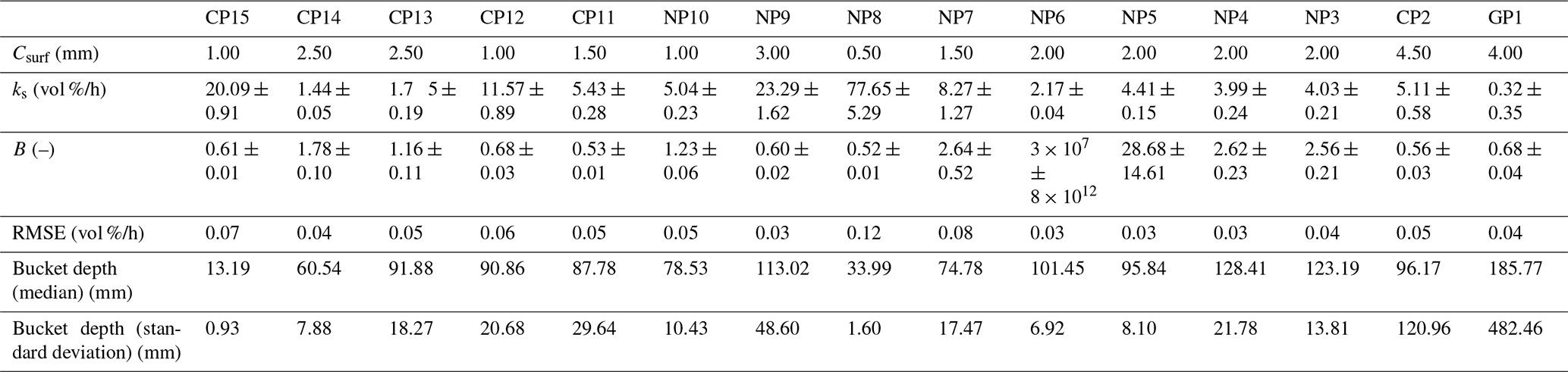
Table A1 Parameters obtained for the plots of the case study. For the drainage model, the standard deviation of the parameters and the root-mean-square error (RMSE) of the fit is included. For the monthly scaling factors, the median and the standard deviation is reported.