the Creative Commons Attribution 4.0 License.
the Creative Commons Attribution 4.0 License.
 | 22 Apr 2021
Porosity and permeability prediction through forward stratigraphic simulations using GPM™ and Petrel™: application in shallow marine depositional settings
David Hodgetts
The forward stratigraphic simulation approach is applied to predict porosity and permeability distribution. Synthetic well logs from the forward stratigraphic model served as secondary data to control porosity and permeability representation in the reservoir model. Building a reservoir model that fits data at different locations comes with high levels of uncertainty. Therefore, it is critical to generate an appropriate stratigraphic framework to guide lithofacies and associated porosity–permeability simulation. The workflow adopted for this task consists of three parts: first, there is simulation of 20 scenarios of sediment transportation and deposition using the geological process modelling (GPM™) software developed by Schlumberger. Secondly, there is an estimation of the extent and proportion of lithofacies units in the stratigraphic model using the property calculator tool in Petrel™. Finally, porosity and permeability values are assigned to corresponding lithofacies units in the forward stratigraphic model to produce a forward stratigraphic-based porosity and permeability model. Results show a forward stratigraphic-based lithofacies model, which depends on sediment diffusion rate, sea-level variation, sediment movement, wave processes, and tectonic events. This observation is consistent with the natural occurrence, where variations in sea level, sediment supply, and accommodation control stratigraphic sequences and therefore facies distribution in a geological basin. Validation wells VP1 and VP2 showed a notable match after a comparing the original and forward stratigraphic-based porosity models. However, a significant discrepancy is recorded in the permeability estimates. These results suggest that the forward stratigraphic modelling approach can be a practical addition to geostatistical-based workflows for realistic prediction of porosity and permeability.
- Article
(7918 KB) - Full-text XML
- BibTeX
- EndNote


The distribution of reservoir properties such as porosity and permeability is a direct function of a complex combination of sedimentary, geochemical, and mechanical processes (Skalinski and Kenter, 2014). The impact of reservoir petrophysics on well planning and production strategies makes it imperative to use reservoir modelling techniques that present realistic property variations via 3-D models (Deutsch and Journel, 1999; Caers and Zhang, 2004; Hu and Chugunova, 2008). Typically, reservoir modelling requires continued property modification until an appropriate match to subsurface data. Meanwhile, subsurface data acquisition is expensive and thus restricts data collection and accurate subsurface property modelling. Several studies, Hodgetts et al. (2004) and Orellana et al. (2014), have demonstrated how stratigraphic patterns, and therefore petrophysical attributes in seismic data, outcrops, and well logs, are applicable in subsurface modelling. However, the absence of detailed three-dimensional depositional frameworks to guide property modelling inhibits the use of stratigraphic patterns to capture subsurface property variations (Burges et al., 2008). Reservoir modelling techniques with the capacity to integrate forward stratigraphic simulation outputs with stochastic modelling techniques for subsurface property modelling will improve reservoir heterogeneity characterization, because they more accurately produce geological realism than the other modelling methods (Singh et al., 2013). The use of geostatistical-based methods to represent spatial variability of reservoir properties has been in many exploration and production projects (Kelkar and Perez, 2002). In the geostatistical modelling method, an alternate numerical 3-D model (realizations) shows different property distribution scenarios that are most likely to match well data (Ringrose and Bentley, 2015). However, due to cost, reservoir modelling practitioners continue to encounter the challenge of obtaining adequate subsurface data to deduce reliable variograms for geostatistical-based subsurface modelling, therefore introducing a significant level of uncertainty in reservoir models (Orellena et al., 2014). The advantages of applying geostatistical modelling approaches to represent subsurface properties in models are discussed in studies by Deutsch and Journel (1999) and Dubrule (1998). A notable disadvantage is that the geostatistical modelling method tends to confine reservoir property distribution to subsurface data and rarely produces geological realism to capture sedimentary events that led to reservoir formation (Hassanpour et al., 2013). In effect, the geostatistical modelling technique does not reproduce long-range continuous reservoir properties, which are essential for generating realistic reservoir connectivity models (Strebelle and Levy, 2008). In their work, Christ et al. (2016) illustrate the use of forward stratigraphic modelling for reconstructing subsurface patterns. The forward stratigraphic modelling method operates on the guiding principle that multiple sedimentary process simulations in a 3-D framework will provide geologic details to improve the modelling of stratigraphic sequences and therefore facies and petrophysical property distribution in an existing basin model. Given this, the forward stratigraphic simulation approach was applied in this contribution to forecast lithofacies, porosity, and permeability in a reservoir model. A significant aspect of this work is using variogram parameters from forward stratigraphic-based synthetic wells to simulate porosity and permeability trends in the reservoir model.
The geological process modelling (GPM™) software (Schlumberger™ Softwares, 2019) is used to replicate sediment depositional processes in the model area to realize realistic stratigraphic sequences for porosity and permeability prediction. The reservoir interval understudy is within the Hugin Formation. Studies by Varadi et al. (1998) and Kieft et al. (2011) indicate that the Hugin Formation was formed through a complex depositional architecture of waves, tidal, and fluvial processes. This knowledge suggests that a single depositional model will not be adequate to produce a realistic lithofacies or petrophysical distributions model of the area. Furthermore, the indication of a complicated syn-depositional rift-related faulting system by Milner and Olsen (1998) significantly influences the stratigraphic architecture of the model area. Therefore, the contribution seeks to produce a depositional sequence which captures subsurface attributes observed in seismic and well data to guide porosity and permeability modelling.
The Volve field (Fig. 1), located in block 15/9 south of the Norwegian North Sea, has the Hugin Formation as the reservoir interval from which hydrocarbons are produced (Vollset and Dore, 1984). The Hugin Formation, which is Jurassic in age (late Bajocian to Oxfordian), is made up of shallow marine to marginal marine sandstone deposits and coals, and a significant influence of wave events that tend to control lithofacies distribution in the formation (Varadi et al., 1998; Kieft et al., 2011). Studies by Sneider et al. (1995) and Husmo et al. (2003) associate sediment deposition with the study area to rift-related subsidence and successive flooding during a large transgression of the Viking Graben within the Middle to Late Jurassic period. Also, Cockings et al. (1992) and Milner and Olsen (1998) indicate that the Hugin Formation comprises marine shoreface, lagoonal and associated coastal plain, back-stepping delta plain, and delta front. However, recent studies by Folkestad and Satur (2008) also provide evidence of a high tidal event, which introduces another dimension that requires attention in any subsurface modelling task in the study area. The thickness of the Hugin Formation is estimated to be between 5 and 200 m but can be thicker off structure and non-existent on structurally high segments due to post-depositional erosion (Folkestad and Satur, 2008).
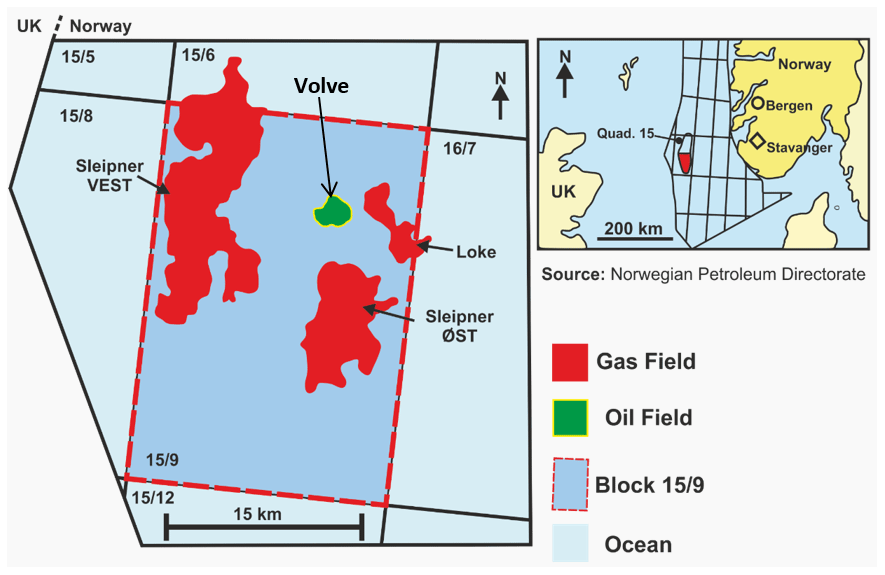
Figure 1Location map of the Volve field showing gas and oil fields in quadrant 15/9, Norwegian North Sea (from Ravasi et al., 2015).
A summarized sedimentological delineation within the Hugin Formation is presented based on studies by Kieft et al. (2011). In Table 1, lithofacies-association codes A, B, C, D, and E represent bay fill units, shoreface sandstone facies, mouth bar units, fluvio-tidal channel fill sediments, and coastal plain facies units, respectively. Additionally, there is a lithofacies-association-prefixed code (F) which consists of open marine shale units and mudstone. Within it are occasional siltstone beds, parallel-laminated soft sediment deformations that locally develop at bed tops. The lateral extent of the code F lithofacies package in the Hugin Formation is estimated to be 1.7 to 37.6 km, but the total thickness of code F lithofacies is not known (Folkestad and Satur, 2008).
Table 1Summarized lithofacies associations in the Hugin Formation, Volve field (after Kieft et al., 2011).

This work is based on the description and interpretation of petrophysical datasets in the Volve field by Equinor. Datasets include 3-D seismic data and a suite of 24 wells that consists of formation pressure data, core data, and petrophysical and sedimentological logs. Previous studies by Folkestad and Satur (2008) and Kieft et al. (2011) in this reservoir interval show varying grain size, sorting, sedimentary structures, and bounding contacts of sediment matrix. Grain size, sediment matrix, and the degree of sorting will typically drive the volume of the void created and therefore the porosity and permeability attributes. Wireline-log attributes such as gamma ray (GR), sonic (DT), density (RHOB), and neutron porosity (NPHI) distinguish lithofacies units, stratigraphic horizons, and zones that are essential for building the 3-D property model in Schlumberger's Petrel™ software. Besides, this study also seeks to produce a realistic depositional model like the natural stratigraphic framework in a shallow marine depositional setting. Therefore, obtaining a three-dimensional stratigraphic model that shows a similar stratigraphic sequence observed in the seismic data allows us to deduce variogram parameters to serve as input in actual subsurface property modelling.
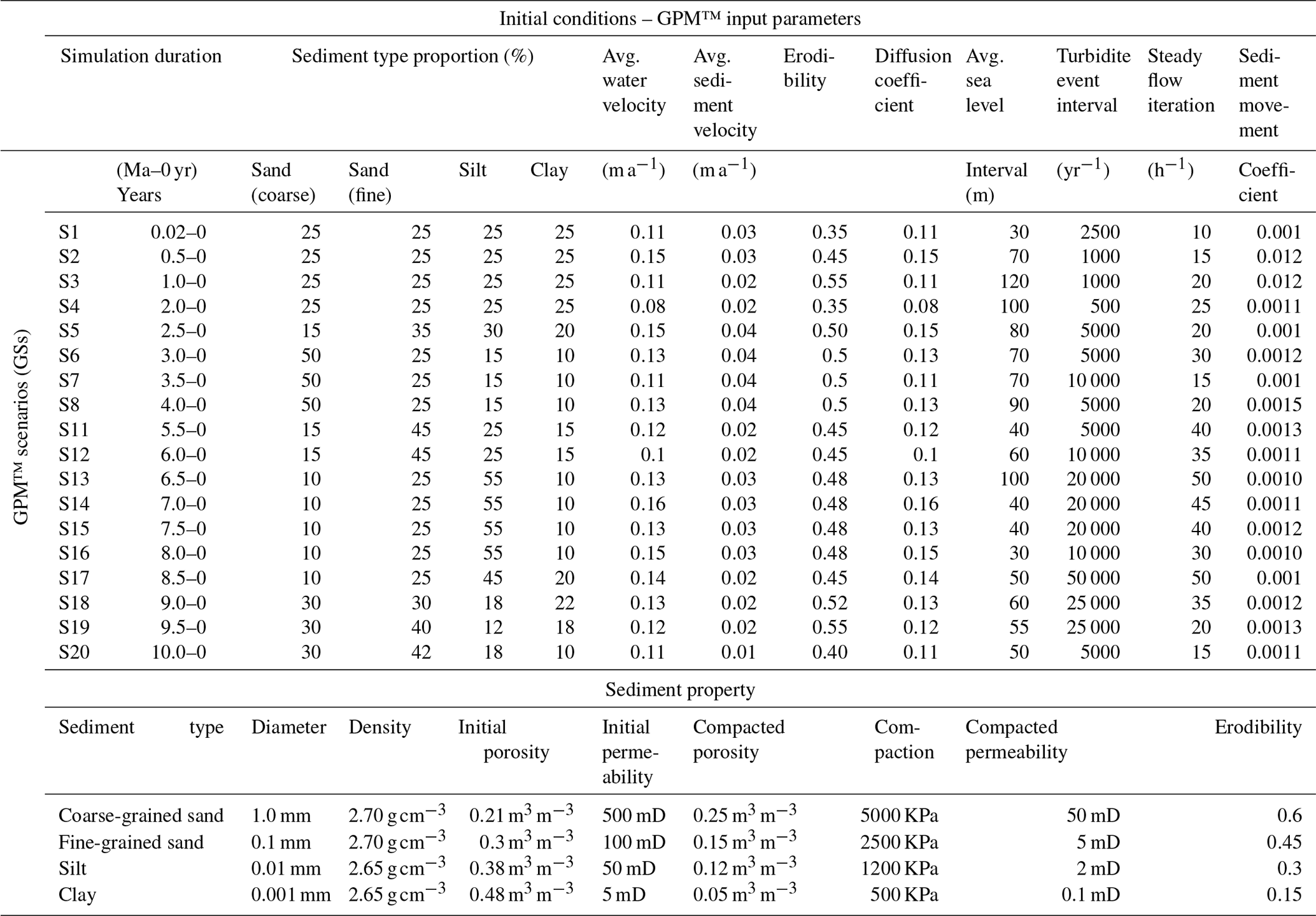
A total of 20 forward stratigraphic simulations were produced in the geological process modelling (GPM™) software to illustrate depositional processes that resulted in the buildup of the reservoir interval under study. By the fourth simulation, there was a development of stratigraphic patterns that shows similar sequences to those observed in seismic data, which led to the decision to constrain the simulation to 20 scenarios. Delft3D-Flow™ and DIONISOS™ are examples of subsurface process modelling software used in previous studies such as Rijn et al. (2003) and Burges et al. (2008). The availability of the GPM™ software license and the capacity to integrate stratigraphic simulation outputs in the property modelling workflow in Petrel™ is the reason for using the geological process modelling software in this study.
3.1 Methodology
The workflow (Fig. 2a) combines the stratigraphic simulation capacity of GPM™ in different sedimentary processes and the property modelling tools in Petrel™ to predict the distribution of porosity and permeability properties away from known data. This involves three broad steps: (i) forward stratigraphic simulation in GPM™ (2019.1 version), (ii) lithofacies classification using the calculator tool in Petrel™, and (iii) porosity and permeability modelling in Petrel™ (2019.1 version).
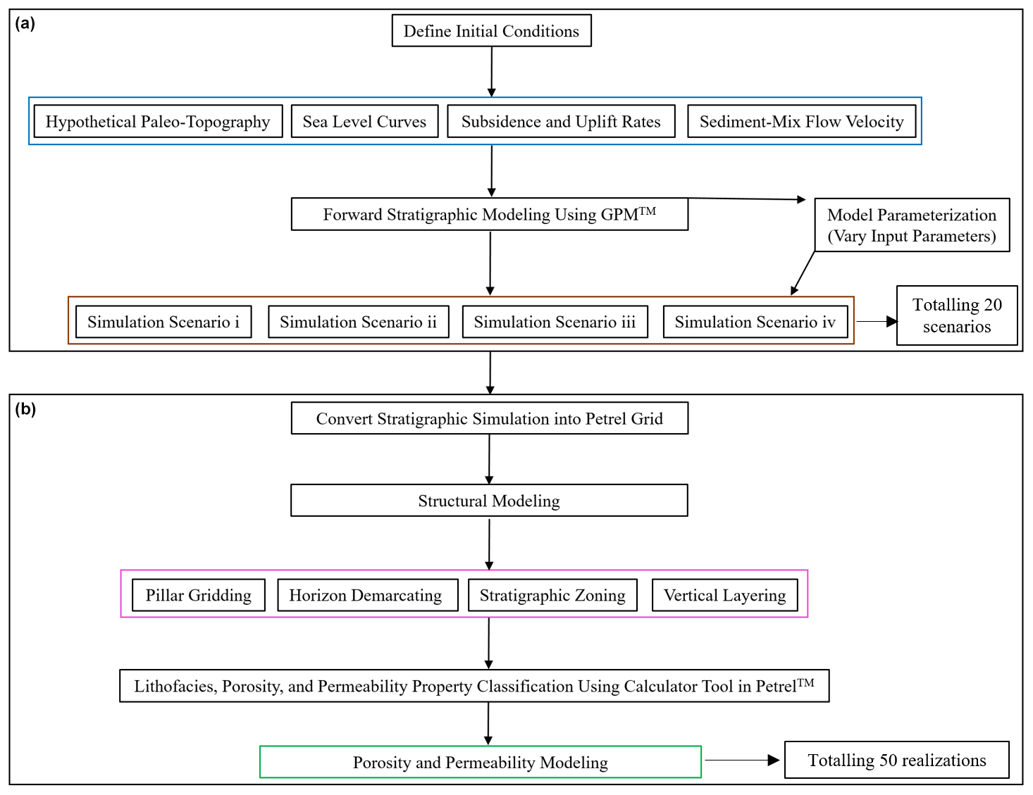
Figure 2Schematic workflow of processes involved in this work. (a) Information of boundary conditions (input parameters) used for the forward stratigraphic simulation in GPM™; (b) illustration of the use of forward stratigraphic models in Petrel™ for porosity and permeability modelling.
3.2 Forward stratigraphic simulation in GPM™
GPM™ is commercial software developed by Schlumberger to simulate clastic and carbonate sedimentation in a deep or shallow marine environment. GPM™ consists of geological processes such as steady flow, sediment diffusion, tectonics, and sediment accumulation that rely on physical equations and assumptions to replicate the process of sedimentation in a geological basin. A realistic realization of a stratigraphic pattern as observed in seismic or well data provides a three-dimensional framework to constrain subsurface property representation that conforms with the real-world property distribution trends. In clastic sedimentation, the movement of sediments relies on equations from the original Sedimentary Simulator (SEDSIM) developed at Stanford University (Harbaugh, 1993). Sediment movement, erosion, and deposition is governed by a simplified Navier–Stokes equation. “Simplified” is used here because the Navier–Stokes equation in its original form defines sediment movement in a three-dimensional differential form, while the flow equation in GPM™ is two-dimensional with an arbitrary input of flow depth. Kieft et al. (2011) describe the influence of a combination of fluvial and wave processes in the genetic structure of sediments in the Hugin Formation. These geological processes are rapid, depending on accommodation generated by sea-level variation and or sediment composition and flow intensity. The deposition of sediments into a geological basin and its response to post-depositional sedimentary or tectonic processes are significant in the ultimate distribution of subsurface lithofacies and petrophysics. Therefore, several input parameters for the forward simulation to attain a stratigraphic output that fits existing knowledge of paleo-sediment transportation and deposition into the study area (see Table 2). The forward simulation at all stages portrayed geological realism concerning stratigraphic sequence, but it also revealed some limitations, such as instability in the simulator when more than three geological processes run concurrently. Given this, the diffusion and tectonic processes remained constant while varying the steady flow, unsteady flow, and sediment accumulation processes in each simulation run.
Table 2Summarized input parameters for forward stratigraphic simulations in GPM™.
3.3 Steady and unsteady flow process
The steady flow process in GPM™ simulates flows that change slowly over a period or sediment transport scenarios where flow velocity and channel depth do not vary abruptly, e.g. rivers at a normal stage, deltas, and sea currents. Considering the influence of fluvial activities during sedimentation in the Hugin Formation, it is significant to capture its impact on the resultant simulated output.
The unsteady flow process can simulate periodic flows such as turbidites where the occurrence is not regular, and the velocity of flow changes abruptly over time. The unsteady flow process applies several fluid elements driven by gravity and friction against the hypothetical topographic surface. Otoo and Hodgetts (2019) illustrate how the unsteady process in GPM™ attains realistic distribution of lithofacies units in a turbidite fan system. Although the steady and unsteady flow governing equations distantly rely on the Navier–Stokes equations, the steady flow is quite distinct, as it uses a finite difference numerical method for faster computation and to also illustrate the frequency of flow that is characteristic in channel flow such as rivers. The finite difference method applies an assumption that flow velocity is constant from channel bottom to the surface. In contrast, the unsteady flow uses the particle method from SEDSIM3 to solve the sediment concentration in flow and sediment transport capacity (Tetzlaff and Harbaugh, 1989). The simplified equation in GPM™ attempts to solve the problem of “shallow-water free-surface flow” over an arbitrary topography surface (Daniel Tetzlaff, personal communication, February 2021). “Shallow water” indicates the instance where only the vertically averaged flow velocity and flow depth are applied and kept track of as a function of two horizontal coordinates.
The equation that controls steady and unsteady flow is expressed through
where h is flow depth, t is time, and Q is the horizontal flow velocity vector.
where is the Lagrangian derivative of flow relative to time, g is gravity, H is the water surface elevation, c2 is the fluid friction coefficient, ρ is the water density, c1 is the water friction coefficient, and h is the flow depth.
Manning's equation is applied to relate flow, slope, flow depth, and hydraulic radius channels with a constant cross section for the steady flow process. Manning's formula states
where V is the flow velocity, k is the unit conversion factor, n is Manning's coefficient which depends on channel rugosity, Rh is the hydraulic radius, and S is the slope.
As mentioned earlier, the unsteady flow process uses the particle method equation, which relies on the assumption that erosion and deposition depend on the balance between the flow's transport capacity and the “effective sediment concentration”. The equation for multiple sediment transport in flow is given as follows:
where Aem is the effective sediment concentration of mixture, lks is the sediment concentration of each type, and f1,ks is the transportability of each sediment type.
The transport capacity of a sediment type is expressed by Eqs. (5) and (6). Let us consider
where f2,ks is the erosion-deposition rate coefficient for sediment type ks. For every sediment type, ks, the formula for transporting sediment of different grain sizes is given as
where H is the free surface elevation to sea level, Z is the topographic elevation for sea level, Ks is the sediment type, and lks is the volumetric sediment concentration of a specific type (k).
3.4 Sediment diffusion process
The diffusion process replicates sediment movement from a higher slope (source location) and deposition into a lower elevation of the model area. Sediment diffusion runs on the assumption that sediments are transported downslope at a proportional rate to the topographic gradient, making fine-grained sediments easily transportable than coarse-grained sediments. Sediment diffusion depends on three parameters: (i) sediment grain size and turbulence in the flow, (ii) diffusion curve that serves as a unitless multiplier in the algorithm, and (iii) diffusion coefficient. The diffusion coefficient depends, among other variables on the type of sediment and “energy” of the depositional environment. In this contribution, the highest depth-dependent diffusion coefficient occurs near sea level, where the “energy” is highest over a geological time (Dashtgard et al., 2007).
In GPM™, sediment diffusion is calculated using a simplified expression:
where z is topographic elevation, Di is the diffusion coefficient, t for time, ∇2z is the Laplacian of z, and Sn is the sediment source term.
Sediment diffusion (Di) is estimated by assuming that the grain sizes for each sediment component (coarse sand, fine sand, silt, and clay) are known. Also an assumption that these sediment types have a uniform diameter (D) in the flow mix (Dade and Friend, 1998; Zhong, 2011). In that case, external fore (Fe), which consist of drag, lift, virtual mass, and Basset history force is given as
Me is the resultant force of other forces with the exception of drag force, Tp Stokes relation time, expressed as , with ρf and Vf as density and viscosity of fluid, respectively. ΦD is a coefficient that accounts for the non-linear dependence of drag force on grain slip Reynolds number (Rp).
With the flow component in place, the diffusion coefficient (Di) is deduced from the Einstein equation. Using an assumption that the diffusion coefficient decreases with increasing grain size and rise in temperature, and that the coefficient f is known, the expression for Di is
Meanwhile, f is a function of the dimension of the spherical particle involved at a particular time (t). In accounting for f, the equation for Di changes into
3.5 Sediment accumulation
The sediment accumulation process in GPM™ is designed to generate an arbitrary amount of sediment representing the artificial vertical thickness of a lithology as interpreted in a well or outcrop data (Daniel Tetzlaff, personal communication, February 2021). The areal input rates for each sediment type (coarse-grained, fine-grained sediments) use the value of the map surface at each cell in the model and multiply it by a value from a unitless curve at each time step in the simulation to estimate the thickness of sediments accumulated or eroded from a cell in the model. Sediment accumulation in the GPM™ software requires other processes such as steady flow and diffusion to account for sediment transport (sediment entering or leaving a cell) before a deposition yr−1 (mm yr−1) function to artificially produce the height of sediment deposited per cell. The accumulation of sediments in GPM™ is expressed as
where AT is the total sediment accumulated in a cell over a period, S is the sediment type, Mv is the map value of sediment in each cell, and SC is the sediment supply curve as a function of topographic elevation.
3.6 Boundary conditions for forward stratigraphic simulation
Realistic reproduction of stratigraphic patterns in the model area requires input parameters (initial conditions), such as paleo-topography, sea-level curves, sediment source location, and distribution curve, tectonic event maps (subsidence and uplift), and sediment mix velocity. The application of these input parameters in GPM™ and their impact on the resultant stratigraphic framework are shown below.
Hypothetical paleo-surface. The hypothetical paleo-topographic for the stratigraphic simulation is from the seismic data (Fig. 3) using the assumption that the present-day stratigraphic surface (paleo-shoreline in Fig. 4a) occurred as a result of basin filling over geological time. Since the surface obtained from the seismic section have undergone various phases of subsidence and uplifts, it is significant to note that the paleo-topographic surface used in this work does not represent an accurate description of the basin at the period of sediment deposition, thus presenting another level of uncertainty in the simulation. To derive an appropriate paleo-topographic for this task, five paleo-topographic surfaces (TPr) were generated by adding or subtracting elevations from the inferred paleo-topographic surface (see Fig. 4g) using the equation
where Sbs is the base surface scenario (in this instance, scenario 6), and EM an elevation below and above the base surface.
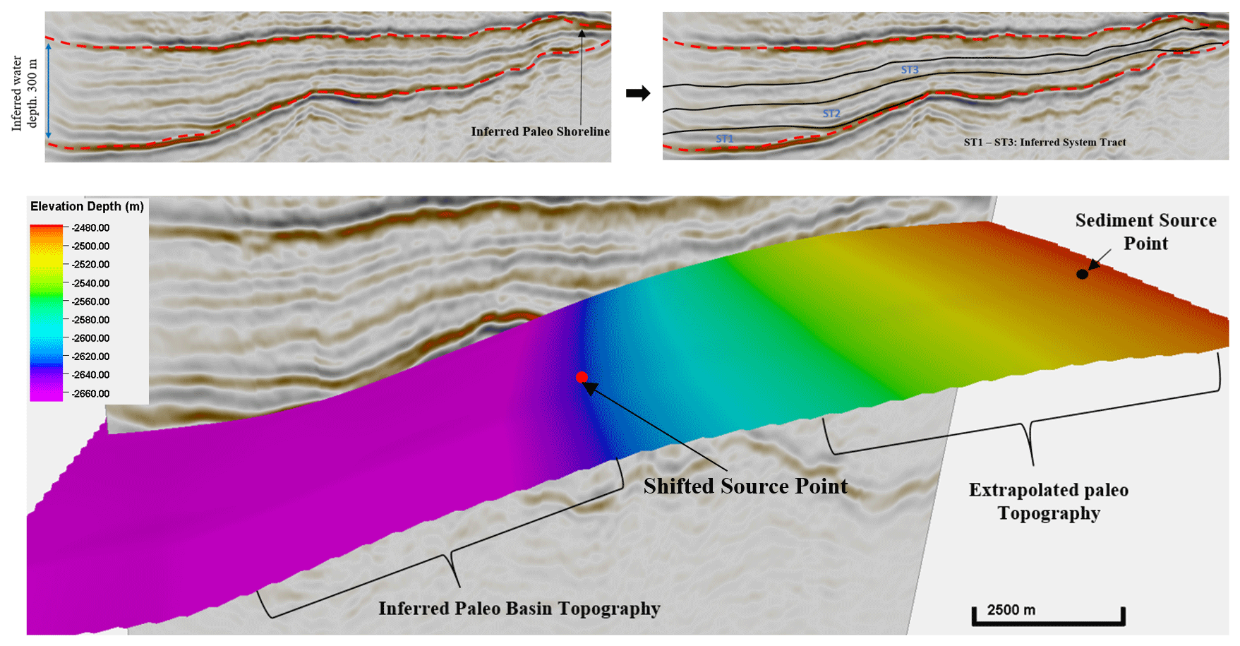
Figure 33-D seismic section of the study area. Hypothetical topographic surface is derived from present-day base of reservoir. The sediment entry point into the basin is located in the northeastern section (based on Kieft et al., 2011).
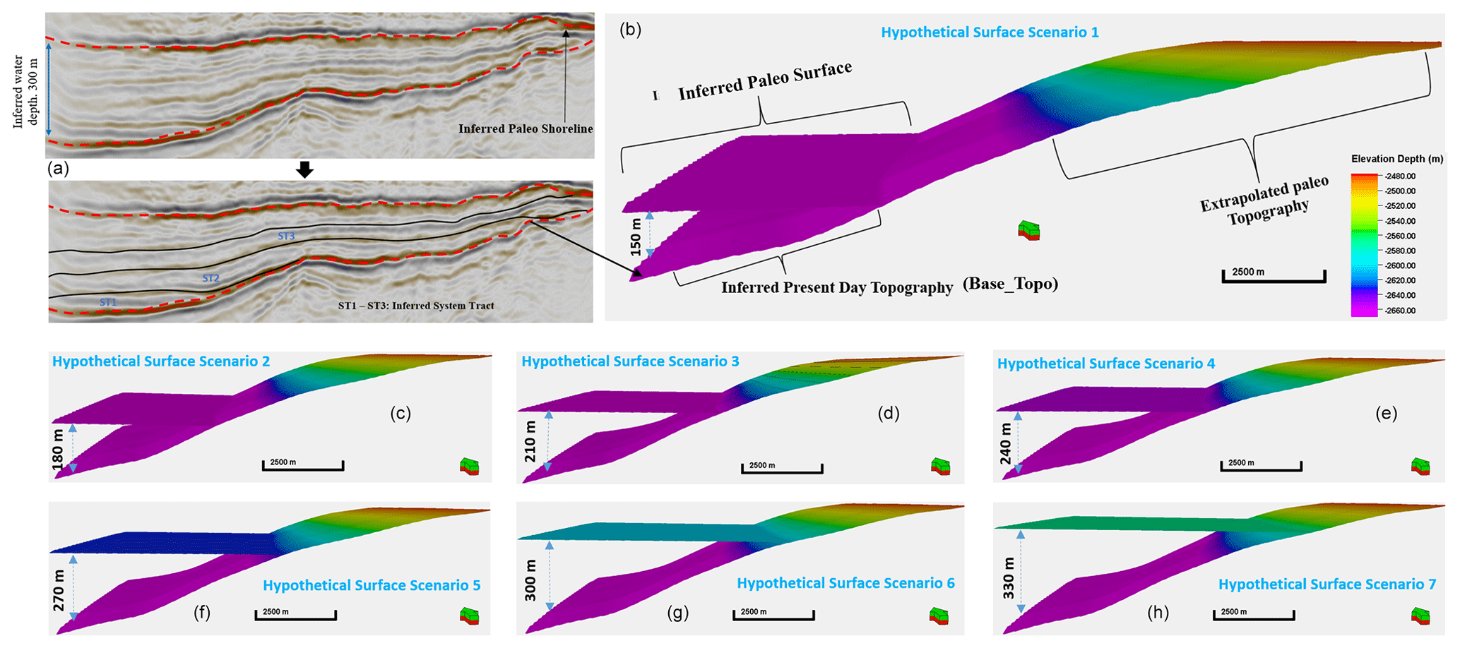
Figure 4Illustration of a range of hypothetical initial topographic surfaces that were used to mitigate the uncertainty in selecting an initial topographic surface for the simulation. Considering that the topographic surface is a key control on stratigraphic sequence, different stratigraphic models are generated to attain a “best-fit” model.
The paleo-topographic surface in scenario 3 (Fig. 4d) is selected because it produced a stratigraphic sequences that fit the depositional patterns interpreted from the seismic section (Fig. 5d).
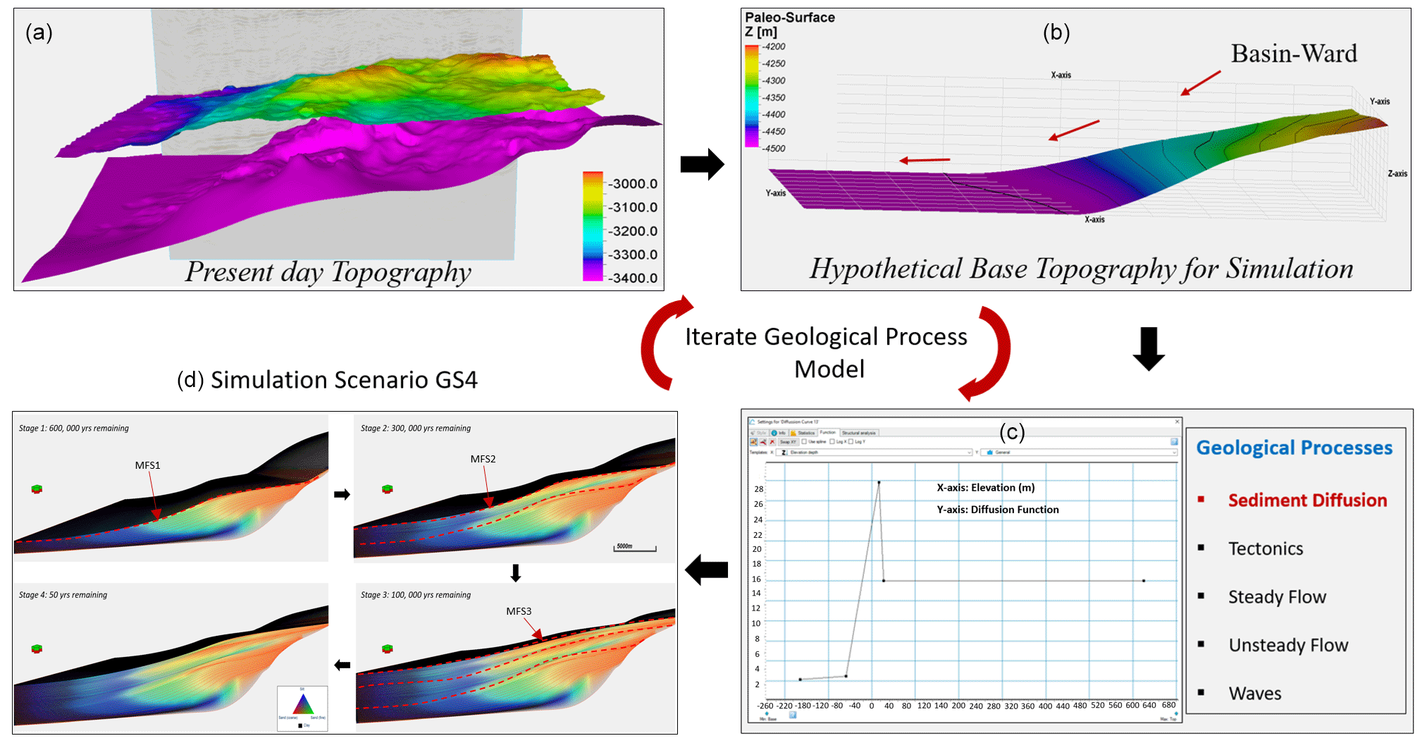
Figure 5(a) Present-day top and bottom topographic surfaces of the Hugin Formation; (b) hypothetical topographic surface after reprocessing of the base reservoir surface; (c) stages of geological processes involved in the forward stratigraphic simulation; (d) forward stratigraphic models at different time intervals of the simulation.
Sediment source location. Based on regional well correlations in Kieft et al. (2011) and seismic interpretation of the basin structure, the sediment entry point is placed in the northeastern section of the hypothetical paleo-topography surface. The exact sediment entry point into this basin is unknown, so three entry points were placed at a 4 km radius around the primary location (Fig. 3c) to capture possible sediment source locations in the model area. The source position is a positive integer (values greater than zero) to enable sediment movement to other parts of the topographic surface.
Sea level. The sea-level curve is deduced from published studies and facies description in shallow marine depositional environments (e.g. Winterer and Bosellini, 1981). The sea level was constrained 30 m for short simulation runs (5000 to 20 000 years) but varied with the increasing duration of the simulation (see Table 2). The peak sea level in the simulation depicts the maximum flooding surface (Fig. 5d) and therefore the inferred sequence boundary in the geological process model.
Diffusion and tectonic event rates. The sediment mix proportion, diffusion rate, and tectonic event functions are from studies such as Walter (1978), Winterer and Bosellini (1981), and Burges et al. (2008). The diffusion and tectonic event rates were increased or reduced to produce a stratigraphic model that fit our knowledge of basin evolution in the study area. For example, in scenario 1 (Fig. 6a), the early stages of clinoform development show resemblance to interpreted trends in the seismic section (Fig. 3b). The process commenced with a diffusion coefficient of 8 m2 a−1, but it varied at each scenario to obtain diffusion coefficients to improve the model. Excluding the initial topography (Fig. 4d), input parameters in geological processes such as wave events, steady or unsteady flow, diffusion, and tectonic events used curve functions to provide variations in the simulation.
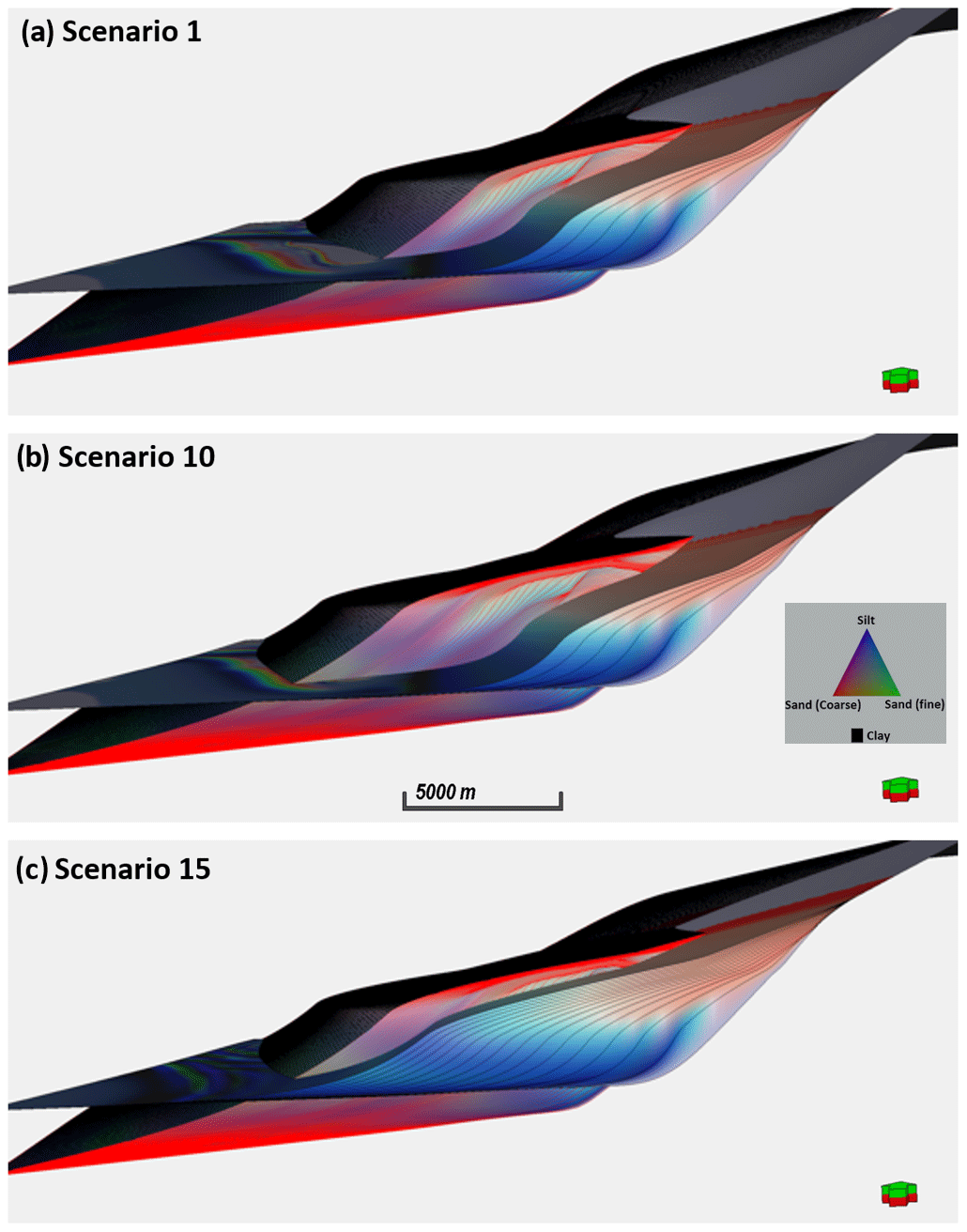
Figure 6Example of stratigraphic simulation scenarios from which the “best-fit” model was selected. Panel (a) involves the use of equal proportions of sediment supply, a relatively low subsidence rate, and low water depth; panel (b) applies a high proportion of fine sand and silt (70 %) in the sediment mix, abrupt changes in subsidence rate, and a relatively high sea level; panel (c) involves very high proportions of fine sand and silt (80 %), a steady rate of subsidence and uplift in the sediment source area, and a relatively low water depth.
The sensitivity of input parameters in the forward stratigraphic simulation is notable when there is a change of value in sediment diffusion and tectonic rates or dimension of the hypothetical topography. For example, a change in sediment source position affects the extent and depth of sediments deposition in the simulation. Shifting the source point to the midsection of the topography (the midpoint of the topography in a basinward direction) resulted in the accumulation of distal elements identical to turbidite lobe systems. This output is consistent with morphodynamic experiments by de Leeuw et al. (2016), where sediment discharge from the basin slope leads to the buildup of basin floor fan units.
In our opinion, the most appropriate output is the stratigraphic model in Fig. 5d. This point of view is because, compared to the depositional description in studies such as Folkestad and Satur (2008) and Kieft et al. (2011), the seismic interpretation presents a similar stratigraphic sequence. Sediment distribution in each time step of the simulation was stacked into a single zone framework to attain a simplified model. This strategy assumes that sedimentary processes that lead to the final buildup of genetic related units within zones of the model will not vary significantly over the simulation period. The stratigraphic model (Fig. 5d) was converted into a 3-D format ( grid cells) for the property modelling in Petrel™.
Facies, porosity, and permeability representation in the stratigraphic model was done via a rule-based approach in Petrel™ (see Table 3). The classification is driven by depositional depth, geologic flow velocity, and sediment distribution patterns as indicated in Fig. 7. Lithofacies representation in the stratigraphic model relied on the sediment grain size pattern and proximity to sediment source. For example, shoreface lithofacies units are medium- to coarse-grained sediments, which accumulate at a proximal distance to the sediment source. In contrast, mudstone units are confined to fine-grained sediments in the distal section of the simulation domain.
Table 3Lithofacies classification in the forward stratigraphic model by using the property calculator tool in Petrel™.
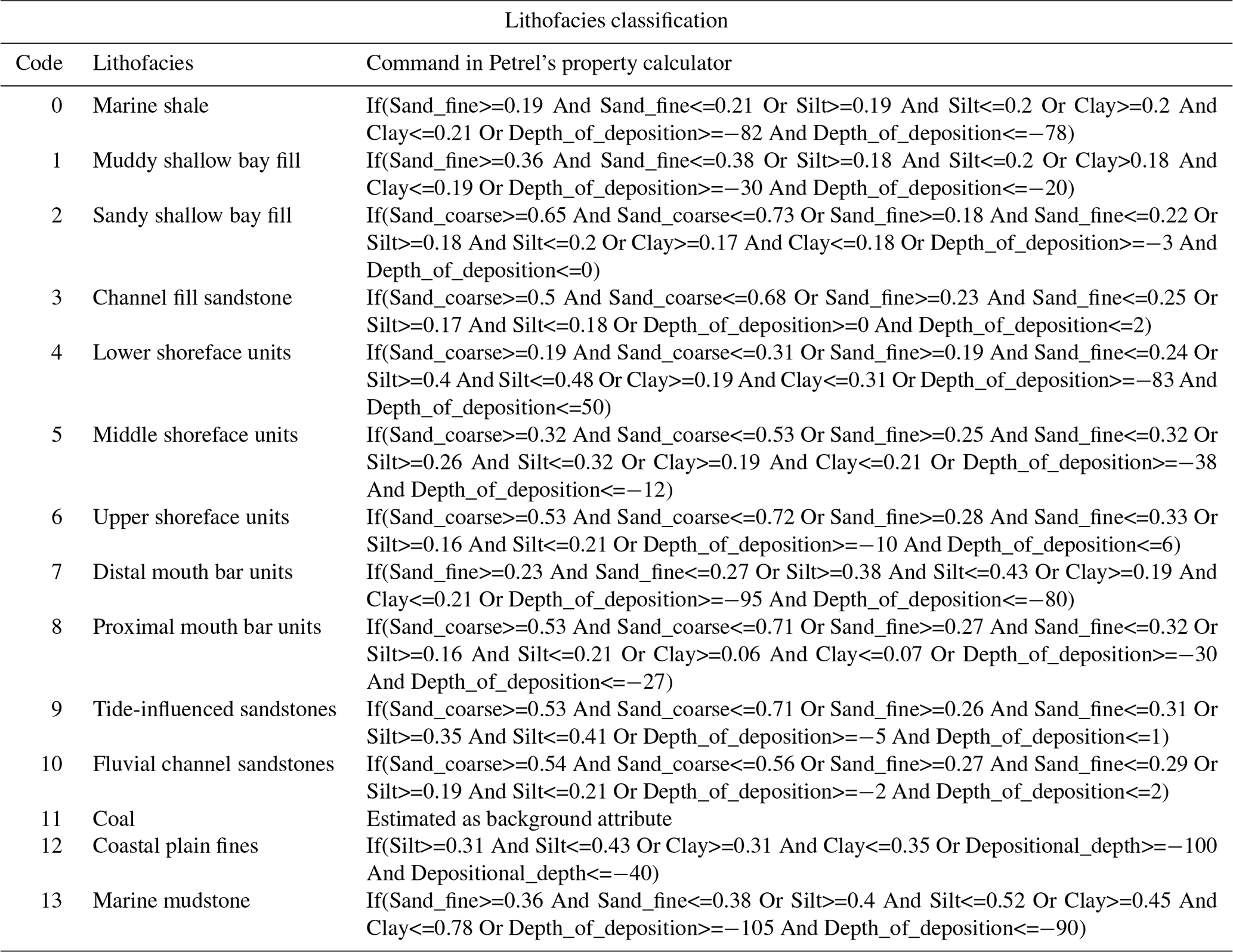
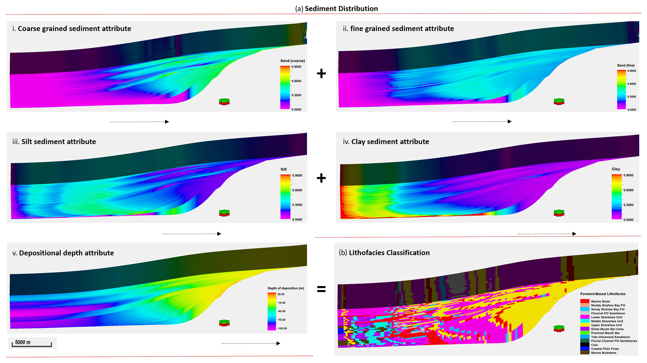
Figure 7(a) Sediment distribution patterns in the geological process modelling software. (b) Lithofacies classification using the property calculator tool in Petrel™.
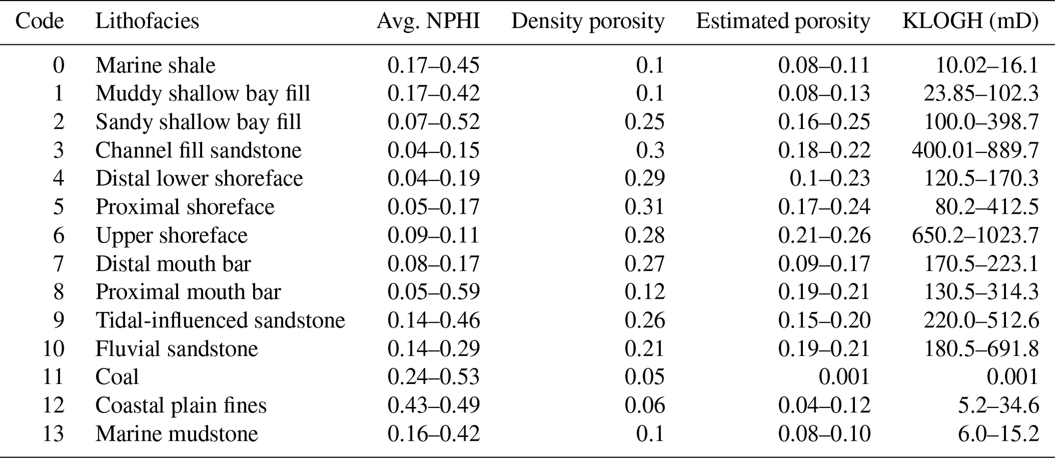
Using knowledge from published studies by Kieft et al. (2011) and wireline-log attributes such as gamma-ray, neutron, sonic, and density logs, porosity and permeability variations in the stratigraphic model are estimated (Table 1). In previous studies on the Sleipner Øst, and Volve field (Equinor, 2006; Kieft et al., 2011), shoreface deposits make up the best reservoir units, while lagoonal deposits formed the worst reservoir units. With this guide, shoreface sandstone units and mudstone and/or shale units in the forward stratigraphic model are best and worst reservoir units, respectively. The porosity and permeability values in Table 4 are from equations in Statoil's petrophysical report of the Volve field (Equinor, 2016):
where Øer is the estimated porosity range, ØD is density porosity, α and β are regression constants ranging between −0.02–0.01 and 0.28–0.4, respectively, NPHI is neutron porosity. In instances where NPHI values for lithofacies units are not available from the published references, an average of 0.25 was used.
where KLOGHer is the estimated permeability range, VSH is the volume of clay and/or shale in the lithofacies unit and PHIF the fractured porosity. The VSH range between 0.01–0.12 for the shoreface units and 0.78–0.88 for lagoonal deposits.
The workflow (Fig. 2b) used for subsurface property modelling in Petrel™ is applied to represent lithofacies, porosity, and permeability properties in the stratigraphic model. These processes involve
-
In structure modelling, identified faults within the study area are modelled together with interpreted surfaces from seismic and well correlation to generate the main structural framework, within which the property model is built. Here, fault pillars and connecting fault bodies are linked to obtain the kind of fault framework interpreted from the seismic data.
-
Pillar gridding involves building a “grid skeleton” made up of a top, middle, and base architectures. Typically, pillars join corresponding corners of every grid cell of the adjacent grid to form the foundation for each cell within the model. The prominent orientation of faults (I direction) within the model area was in an N–S and NE–SW direction, so the “I direction” was set to NNE–SSW to capture the general structural description of the area.
-
With horizons, zones, and vertical layering, stratigraphic horizons and subdivisions (zones) delineate the geological formation's boundaries. As stratigraphic horizons are introduced into the model grid, the surfaces are trimmed iteratively and modified along faults to correspond with displacements across multiple faults. Vertical layering shows the thicknesses and orientation between the layers of the model. Layers refer to significant changes in particle size or sediment composition in a geological formation. Using a vertical layering scheme makes it possible to honour the fault framework, pillar grid, and horizons. A constant cell thickness of 1 m is used in the model to control the vertical scale of lithofacies, porosity, and permeability modelling.
-
Upscaling involves the substitution of smaller grid cells with coarser grid cells. Here, log data are transformed from a one-dimensional to a three-dimensional framework to evaluate which discrete value suits selected data point in the model. One advantage of the upscaling procedure is to make the modelling process faster.
5.1 Porosity and permeability modelling
The Volve field petrophysical model from Equinor is the base (reference) model in this work. The model, which covers 17.9 km2, was generated with the reservoir management software (RMS) developed by Irap and Roxar (Emerson™). The petrophysical model has a grid dimension of and was compressed by 75.27 % of cell size from an approximated cell size of . To achieve a comparable model resolution to the Volve field porosity and permeability model, the forward stratigraphic output, which had an initial resolution of , is upscaled to a grid of . Variograms being a critical aspect of this work, we submit two options to extrapolate variogram parameters from the forward stratigraphic-based porosity and permeability models. In option 1, the porosity and permeability values were assigned to the synthetic lithofacies wells that correlate with known facies association in the study area (see Table 4).
Table 4Porosity and permeability estimates of lithofacies packages in the model area.
The pseudo-wells comprising porosity and permeability are situated in between well locations to guide porosity and permeability simulation in the model. For option 2, the best-fit forward stratigraphic model changes by assigning porosity and permeability attribute using the general stratigraphic orientation captured in the seismic data (NE–SW; 240∘). Porosity and permeability pseudo-(synthetic) logs were then extracted from the forward stratigraphic output to build the porosity and permeability models (Fig. 8). Porosity modelling is through normal distribution, while the permeability models were produced using a log-normal distribution and the corresponding porosity property for collocated co-kriging.
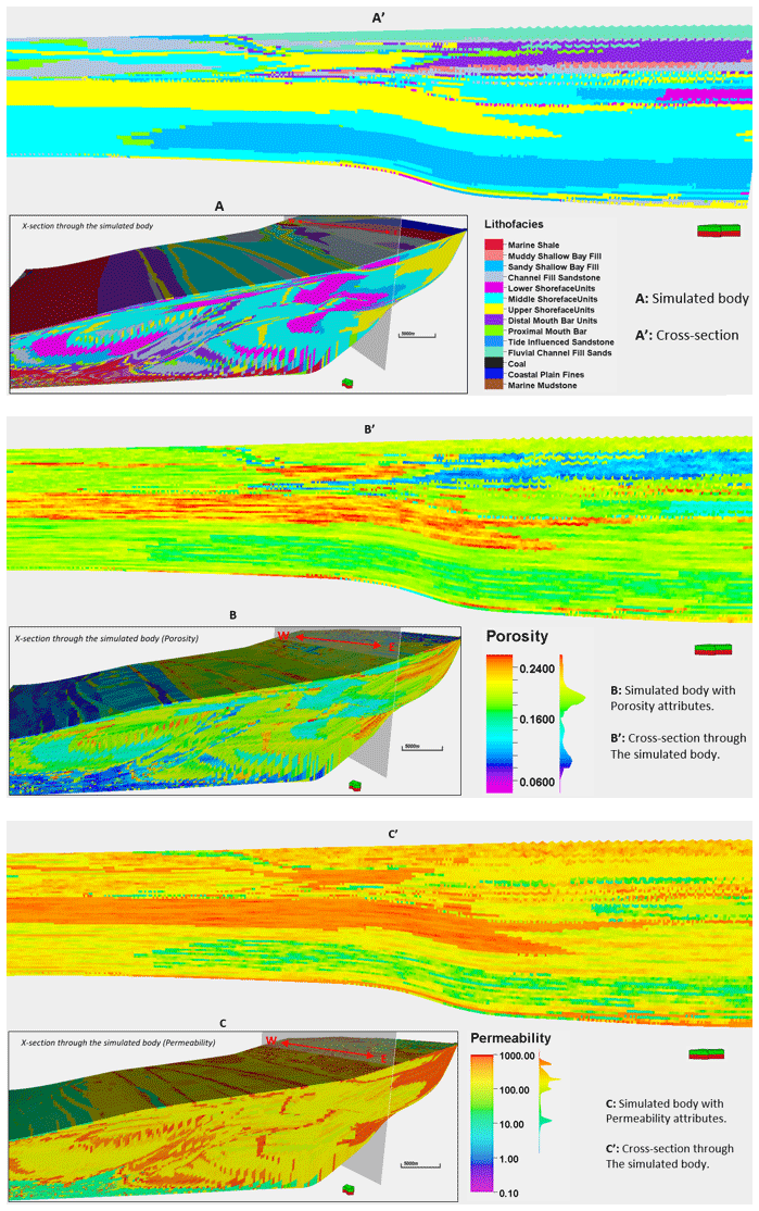
Figure 8Lithofacies, porosity, and permeability trends in the forward stratigraphic-based models.
Considering that vertical trends in options 1 and 2 will be similar within a sampled interval, option 2 presented a viable 3-D representation of property variations in the major and minor directions of the forward stratigraphic model. In total, 10 synthetic wells (SWs), ranging between 80 and 120 m in total depth (TD), are positioned in the forward model to capture the vertical distribution of porosity–permeability at different sections of the forward stratigraphic-based models.
The synthetic wells (Fig. 9c) with porosity and permeability data were upscaled and distributed into the original structural model using the sequential Gaussian simulation method. The synthetic wells derived from the stratigraphic model served as an additional control for porosity and permeability modelling in the Volve field. Because the variogram-based modelling approach is efficient in subsurface data conditioning, this idea presents an opportunity to get more wells at no additional cost to control porosity and permeability distribution. The variogram model (Fig. 10) of dominant lithofacies units in the stratigraphic model served as a guide in estimating variogram parameters for porosity and permeability modelling. The variogram has major and minor ranges of 1400 and 400 m, respectively, and an average sill value of 0.75. Six out of 50 model realizations that show some similarity to the original porosity and permeability model formed the basis of our analysis (Fig. 11). The selection of six realizations was on a visual and statistical comparison of zones in the original Volve field model and the stratigraphic-based porosity–permeability model. The statistical approach involved summary statistics from the reference model and the stratigraphic-based porosity–permeability model. In contrast, the visual evaluation compared the geological realism of forward stratigraphic-based realizations to the base model.
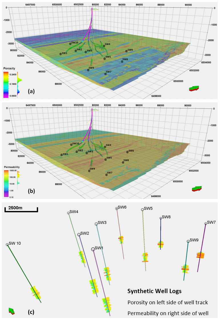
Figure 9Synthetic well forward stratigraphic-based porosity and permeability models. The average separation distance between wells is about 0.9 km.
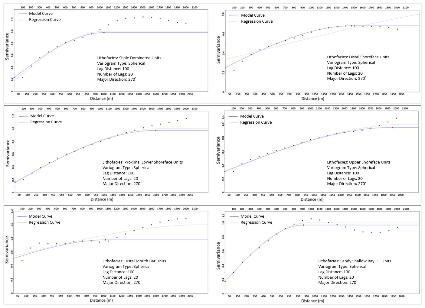
Figure 10Variogram model of dominant lithofacies units from the forward stratigraphic model. The “dots” indicate the number of lags in the variogram through the major direction (NE–SW) of the stratigraphic model.
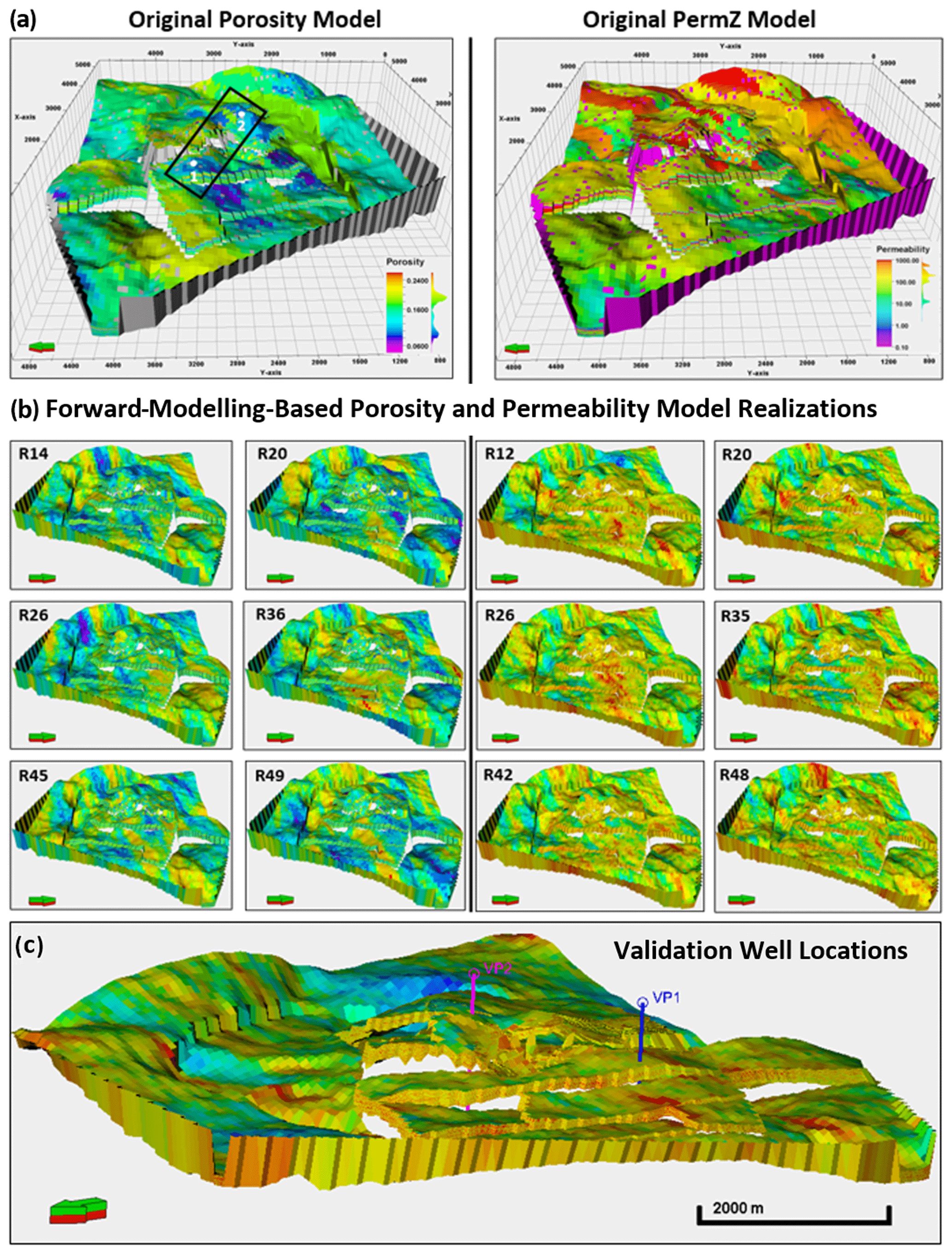
Figure 11Comparing the original Volve vs. the forward-modelling-based porosity and permeability models. Realizations 16, 20, 26, 36, 45, and 49 on the left half are porosity models, while realizations 12, 20, 26, 35, 42, and 48 on the right half are permeability models.
The stratigraphic model in Fig. 5d (stage 4) shows the final geometry after 700 000 years of simulation time. The initial stratigraphic simulation produced a progradation sequence with foreset-like features (stage 1; Fig. 5d) and a sequence boundary, which separates the initial simulated output from the next prograding phase (stage 2). An aggradational stacking pattern commences and becomes prominent in stage 3. These aggradational sequences observed in the forward stratigraphic model are consistent with natural events where sediment supply matchup with accommodation due to sea-level rise within a geological period (Muto and Steel, 2000; Neal and Abreu, 2009).
The impact of the forward stratigraphic simulation on porosity and permeability representation in the reservoir model is evident by comparing its outcomes to the Volve field porosity and permeability models by using two synthetic wells (VP1 and VP2) sampled at a 5 m vertical interval. Taking into account the fact that the Volve field petrophysical model (Fig. 11a) went through various phases of history matching to obtain a model to improve well planning and production strategies, it is reasonable to assume that porosity and permeability distribution in the petrophysical model will be geologically realistic and less uncertain. This view formed the basis for using the porosity and permeability models developed by Equinor as a reference for comparing outputs in the stratigraphic model. Table 5a shows an almost good match in porosity at different intervals in the forward stratigraphic-based models (i.e. R14, R20, R26, R36, R45, and R49). An analysis of the well logs in the model area shows that a large proportion of reservoir porosity is between 0.18–0.24. Also, the analysis of the forward stratigraphic-based porosity model is consistent with the porosity range in the Volve field model (see Fig. 12).
Table 5A comparison of (a) porosity and (b) permeability estimates from selected intervals in the original porosity–permeability models and forward-modelling-based porosity and permeability models.

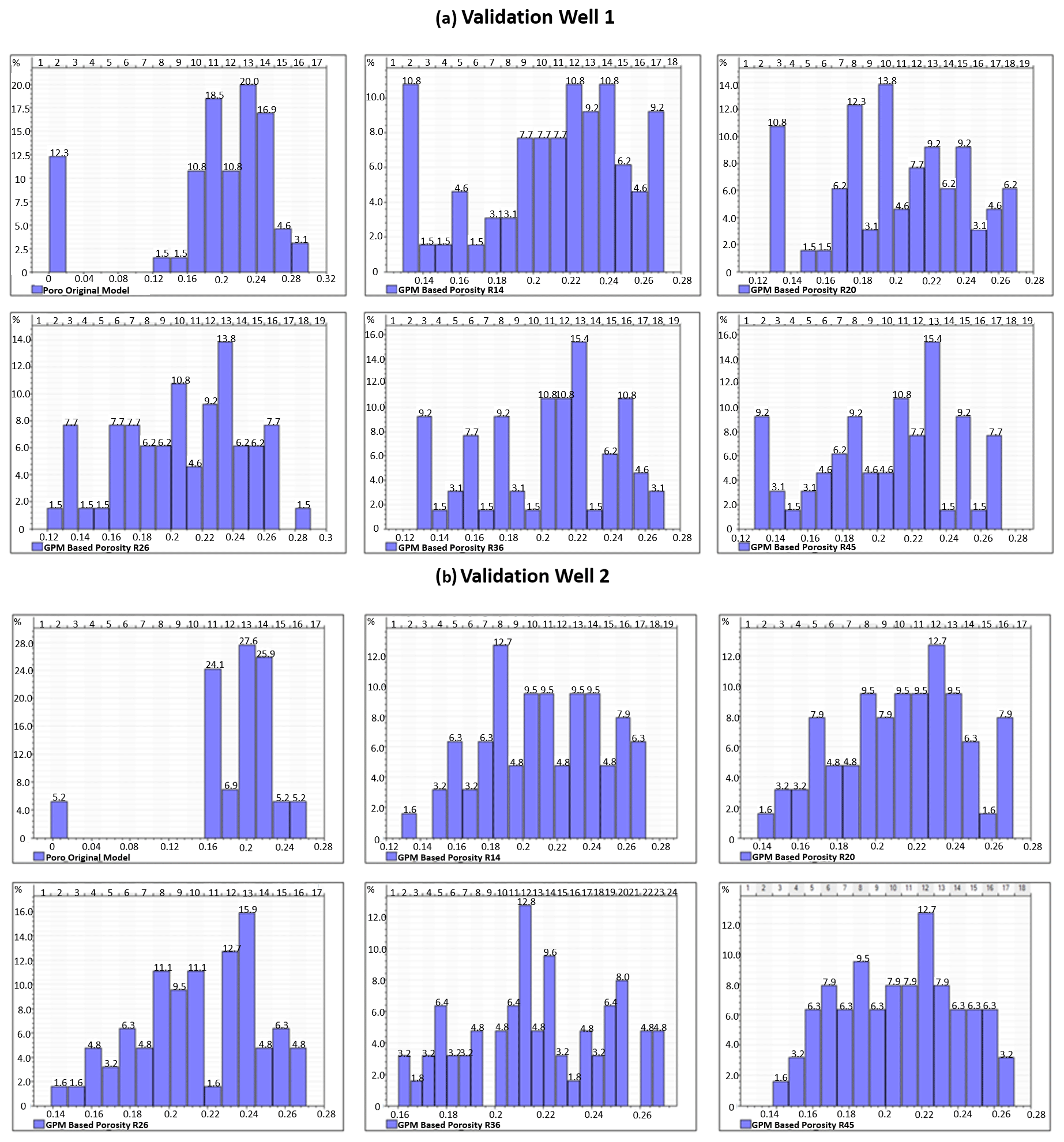
Figure 12Histogram illustrating porosity distribution in validation wells 1 and 2 of five stratigraphic-based realizations and the original porosity model at identical vertical intervals.
A notable limitation with this approach is the assumption that variogram parameters and stratigraphic inclination within zones remained constant throughout the simulation. The difference in permeability attributes between the original permeability model and the forward stratigraphic-based type is the application of other measured parameters in the original model (Table 5b). Typically, a petrophysical model like the Sleipner Øst and Volve field model will factor in other datasets such as special core analysis (SCAL) and level of cementation, which enhances reservoir petrophysics assessment. Bearing in mind that the forward stratigraphic model did not involve some of this additional information from the reservoir, it is practicable to suggest that results obtained in the forward stratigraphic-based porosity and permeability models have been adequately conditioned to known subsurface data.
Results show the influence of sediment transport rate (or diffusion rate), initial basin topography, and sediment source location on the stratigraphic simulation in GPM™. Compared to studies such as Muto and Steel (2000) and Neal and Abreu (2009), we observed that a variation in sea-level controls the volume of sediment that is retained or transported further into the basin, therefore controlling the resultant stratigraphic sequences. In related work, Burges et al. (2008) suggest that a sediment-wedge topset width connects directly to the initial bathymetry, in which the sediment-wedge structure develops, and the correlation between sediment supply and accommodation rate. This opinion is in line with observations in this study, where the initial sediment deposit controls the geometry of subsequent phases of depositions in the hypothetical basin. The uncertainty of initial conditions used in this work led to the generation of multiple forward stratigraphic scenarios to account for the range of bathymetries that may have influenced sediment transportation to form the present-day reservoir units in the Volve field.
The simulation produced well-defined sloping depositional surfaces in a stratigraphic architecture (clinoforms) and sequence boundaries that depict patterns seen in the seismic data. In their work, Allen and Posamentier (1993) and Ghandour and Haredy (2019) explained the importance of sequence stratigraphy in lithofacies characterization and therefore petrophysical property distribution in sedimentary systems. Also, sediment deposition into a geological basin in the natural order is controlled by mechanical and geochemical processes that modify petrophysical attributes (Warrlich et al., 2010); therefore, using different geological processes and initial conditions to generate depositional scenarios in 3-D provides a framework to analyse property variations in a hydrocarbon reservoir. The approach produces a porosity–permeability model comparable to the original petrophysical model using synthetic porosity and permeability logs from the forward stratigraphic model as input datasets. As mentioned, this work did not include variations in the layering scheme that develops in different zones of the stratigraphic model. Under this circumstance, there is a possibility to overestimate and or underestimate porosity and permeability property in some sampled intervals in the validation wells. Therefore, we suggest that the forward stratigraphic simulation outputs such as the example presented in this contribution serve as additional data to understand sediment distribution patterns and associated vertical and horizontal petrophysical trends in the depositional environment and not as absolute conditioning data in subsurface property modelling.
The assumptions made concerning the type of geological processes and input parameters in the stratigraphic simulation certainly differ from what existed during sediment deposition. So, applying stratigraphic models that fit a basin-scale description to a relatively smaller-scale reservoir presents another level of uncertainty in this approach. This opinion agrees with Burges et al. (2008), where they indicate that the diffusion geological process simulation fits the description of large-scale sediment transportation. This view further buttresses the point that integrating forward stratigraphic simulation into a well-scale framework has a high chance of producing outcomes that deviate from the real-world subsurface description. In line with observations in Bertoncello et al. (2013), Aas et al. (2014), and Huang et al. (2015) in relation to limitations in the forward stratigraphic simulation method, it is advisable to use its outputs cautiously in reservoir modelling; as such, outputs from forward stratigraphic models could lead to an increase in property representation bias in a model.
The correlation between reservoir lithofacies and petrophysics, and its prediction through reservoir models, has been extensively examined in several studies (Falivene et al., 2006; Hu and Chugunova, 2008). Meanwhile, the predicted outputs most often do not depict the actual reservoir character due to the absence of a realistic 3-D stratigraphic framework to guide reservoir property representation in geological models. The forward stratigraphic modelling method, notwithstanding its limitations, provides reservoir modelling practitioners a platform to generate subsurface models that reflect the natural variation of reservoir properties.
In this paper, synthetic well data from a forward stratigraphic simulation are combined with well data from the Volve field to predict porosity and permeability distribution. The forward stratigraphic modelling scenarios presented in this work do not prove that forward stratigraphic outputs should be used as absolute input parameters for a real-world reservoir modelling task. Considering the uncertainties highlighted in the choice of initial boundary conditions and geological processes for the stratigraphic simulation, it is notable that the simulation produced a depositional architecture that is geologically realistic and comparable to the stratigraphic correlation suggested in published studies of the study area. The match in porosity obtained by comparing validation wells in the original and stratigraphic-based petrophysical model indicates that it is practical to use variogram parameters and or well data from forward stratigraphic simulations for reservoir property modelling. This work also made two key findings:
-
For specific stratigraphic simulation in GPM™ and a range of model parameters, sediment transportation and deposition are based on diffusion rate and proximity to the sediment source. This opinion agrees with several published works on sequence stratigraphy and or system tracts in shallow marine settings. However, further work with different forward stratigraphic modelling simulators could mitigate some of the challenges faced in this work.
-
A lithofacies distribution that is consistent with previous studies was produced in the stratigraphic model. This is evident in model scenarios where sediment distribution vertically matches with lithofacies variation in a sampled interval in an actual well log.
-
Geologically feasible stratigraphic patterns generated in the forward stratigraphic model provide an additional layer of confidence in representing facies distribution and therefore porosity–permeability variations in a subsurface model. Furthermore, the resultant forward stratigraphic-based porosity and permeability model suggests that forward stratigraphic modelling can be integrated into geostatistical modelling workflows to improve subsurface property modelling and well planning.
The dataset for this work is from Equinor (Volve field, Norway) and was made available to the public in 2018. The data include 24 suits of well logs and 3-D reservoir models in Eclipse and RMS formats. The data, models (eclipse and RMS formats), and the rule-based calculation script to generate lithofacies and porosity–permeability proportions are archived on Zenodo (https://doi.org/10.5281/zenodo.3855293) as Otoo and Hodgetts (2020).
The (2019.1) version of GPM™ software was used in completing this work after an initial 2018.1 version. It is available at https://www.software.slb.com/products/gpm (last access: 1 March 2021). The software license and code used in the GPM™ cannot be provided, because Schlumberger does not allow the code for its software to be shared in publications.
The work started in Petrel™ software (2017.1), but it was completed with Petrel™ software (2019.1). The software is available at https://www.software.slb.com/products/petrel (last access: 1 March 2021). The software runs on a Windows PC with the following specifications: processor: Intel Xeon CPU E5-1620 v3 at 3.5 GHz, four cores, eight threads; memory: 64 GB RAM. The computer should be high end, because a lot of processing time is required for the task. The forward stratigraphic models are on Zenodo (https://doi.org/10.5281/zenodo.3855293) as Otoo and Hodgetts (2020).
DO designed the model workflow, conducted the simulation using the GPM™ software, evaluated the results, and drafted the manuscript. DH converted the Volve field data into Petrel-compatible format and assisted in the revision of the manuscript.
The authors thank Equinor for making the Volve field dataset available. The authors also thank Schlumberger for providing the GPM™ software license. A special thanks is given to Mostfa Legri and Daniel Tetzlaff (Schlumberger) for their technical support in the use of GPM™. Finally, the authors thank the Ghana National Petroleum Corporation (GNPC) for sponsoring this research.
This paper was edited by Andrew Yool and reviewed by Brian Burham and one anonymous referee.
Aas, T., Basani, R., Howell, J., and Hansen, E.: Forward modeling as a method for predicting the distribution of deep-marine sands: an example from the Peira Cava sub-basin, Geol. Soc. Sp., 387, 247–269, https://doi.org/10.1144/SP387.9, 2014.
Allen, G. P. and Posamentier, H. W.: Sequence stratigraphy and facies model of an incised valley fill, the Gironde Estuary, France, J. Sediment. Res., 63, 378–391, https://doi.org/10.1306/D4267B09-2B26-11D7-8648000102C1865D, 1993.
Bertoncello, A., Sun, T., Li, H., Mariethoz, G., and Caers, J.: Conditioning Surface-Based Geological Models to Well and Thickness Data, International Association of Mathematical Geoscience, 45, 873–893, https://doi.org/10.1007/s11004-013-9455-4, 2013.
Burges, P. M., Steel, R. J., and Granjeon, D.: Stratigraphic Forward Modeling of Basin-Margin Clinoform Systems: Implications for Controls on Topset and Shelf Width and Timing of Formation of Shelf-Edge deltas. Recent advances in models of siliciclastic shallow-marine stratigraphy, SEPM Spec. P., 90, 35–45, 2008.
Caers, J. and Zhang, T.: Multiple-point geostatistics: a quantitative vehicle for integrating geologic analogs into multiple reservoir models, in: Integration of outcrop and modern analogs in reservoir modeling, edited by: Grammer, G. M., Harris, P. M., and Eberli, G. P., AAPG Memoir, 384–394, 2004.
Christ, A., Schenk, O., and Salomonsen, P.: Using Stratigraphic Forward Modeling to Model the Brookian Sequence of the Alaska North Slope, in: Geostatistical and Geospatial Approaches for the Characterization of Natural Resources in the Environment, edited by: Raju, N., Springer, Cham, New York, https://doi.org/10.1007/978-3-319-18663-4_94, 2016.
Cockings, J. H., Kessler, L. G., Mazza, T. A., and Riley, L. A.: Bathonian to mid-Oxfordian Sequence Stratigraphy of the South Viking Graben, North Sea, Geol. Soc. Sp., 67, 65–105, https://doi.org/10.1144/GSL.SP.1992.067.01.04, 1992.
Dade, W. B. and Friend, P. F.: Grain Size, Sediment Transport Regime, and Channel Slope in Alluvial Rivers, J. Geol., 106, 661–676, 1998.
Dashtgard, S. E., White, R. O., Butler, K. E., and Gingras, M.: Effects of relative sea level change on the depositional character of an embayed beach, Bay of Fundy, Canada, Mar. Geol., 239, 143–161, 2007.
De Leeuw, J., Eggenhuisen, J. T., and Cartigny, M. J. B.: Morphodynamics of submarine channel inception revealed by new experimental approach, Nat. Commun., 7, 10886, https://doi.org/10.1038/ncomms10886, 2016.
Deutsch, C. and Journel, A.: GSLIB. Geostatistical software library and user's guide, Geol. Mag., 136, 83–108, https://doi.org/10.2307/1270548, 1999.
Dubrule, O.: Geostatistics in Petroleum Geology, AAPG, 38, 27–101, https://doi.org/10.1306/CE3823, 1998.
Equinor: Sleipner Øst, Volve Model, Hugin and Skagerrak Formation Petrophysical Evaluation, Stavanger, Norway, available at: https://data.equinor.com/dataset/Volve (last access: 20 April 2021), 2006.
Falivene, O., Arbues, P., Gardiner, A., and Pickup, G. E.: Best practice stochastic facies modeling from a channel-fill turbidite sandstone analog (the Quarry outcrop, Eocene Ainsa basin, northeast Spain, AAPG, 90, 1003–1029, https://doi.org/10.1306/02070605112, 2006.
Folkestad, A. and Satur, N.: Regressive and transgressive cycles in a rift-basin: Depositional model and sedimentary partitioning of the Middle Jurassic Hugin Formation, Southern Viking Graben, North Sea, Sediment. Geol., 207, 1–21, https://doi.org/10.1016/j.sedgeo.2008.03.006, 2008.
Ghandour, I. M. and Haredy, R. A.: Facies Analysis and Sequence Stratigraphy of Al-Kharrar Lagoon Coastal Sediments, Rabigh Area, Saudi Arabia: Impact of Sea-Level and Climate Changes on Coastal Evolution, Arab. J. Sci. Eng., 44, 505–520, 2019.
Harbaugh, J. W.: Simulating Sedimentary Basins: An Overview of the SEDSIM Model and its Relevance to Sequence Stratigraphy, Geoinformatics, 4, 123–126, 1993.
Hassanpour, M., Pyrcz, M., and Deutsch, C.: Improved geostatistical models of inclined heterolithic strata for McMurray formation, Canada, AAPG Bull., 97, 1209–1224, https://doi.org/10.1306/01021312054, 2013.
Hodgetts, D. D., Drinkwater, N. D., Hodgson, J., Kavanagh, J., Flint, S. S., Keogh, K. J., and Howell, J. A.: Three-dimensional geological models from outcrop data using digital data collection techniques: an example from the Tanqua Karoo depocenter, South Africa, Geol. Soc. Sp., 171, 57–75, https://doi.org/10.1144/GSL.SP.2004.239.01.05, 2004.
Hu, L. Y. and Chugunova, T.: Multiple-point geostatistics for modeling subsurface heterogeneity: A comprehensive review, Water Resour. Res., 44, 1–14, https://doi.org/10.1029/2008WR006993, 2008.
Huang, X., Griffiths, C., and Liu, J.: Recent development in stratigraphic forward modeling and its application in petroleum exploration, Aust. J. Earth Sci., 62, 903–919, https://doi.org/10.1080/08120099.2015.1125389, 2015.
Husmo, T., Hamar, G. P., Høiland, O., Johannessen, E. P., Rømuld, A., Spencer, A. M., and Titterton, R.: Lower and Middle Jurassic, in: The Millennium Atlas: Petroleum Geology of the Central and Northern North Sea, edited by: Evans, D., Graham, C., Armour, A., and Bathurst, P., Geological Society, London, 129–155, 2003.
Kelkar, M. and Perez, G.: Applied Geostatistics for Reservoir Characterization, Society of Petroleum Engineers, Applied Geostatistics for Reservoir characterization, https://www.academia.edu/36293900/ (last access: 10 September 2019), 2002.
Kieft, R. L., Jackson, C. A.-L., Hampson, G. J., and Larsen, E.: Sedimentology and sequence stratigraphy of the Hugin Formation, Quadrant 15, Norwegian sector, South Viking Graben, AAPG Conference Series, 7, 157–176, https://doi.org/10.1144/0070157, 2011.
Milner, P. S. and Olsen, T.: Predicted distribution of the Hugin Formation reservoir interval in the Sleipner Østfield, South Viking Graben, the testing of a three-dimensional sequence stratigraphic model, in: Sequence Stratigraphy; Concepts and Applications, edited by: Gradstein, F. M., Sandvik, K. O., and Milton, N. J., NPF Sp. Publ., 8, 337–354, 1998.
Muto, T. and Steel, R. J.: The accommodation concept in sequence stratigraphy: Some dimensional problems and possible redefinition, Geology, 130, 1–10, 2000.
Neal, J. and Abreu, V.: Sequence stratigraphy hierarchy and the accommodation succession method, Geology, 37, 779–782, 2009.
Orellana, N., Cavero, J., Yemez, I., Singh, V., and Sotomayor, J.: Influence of variograms in 3D reservoir-modeling outcomes: An example, The Leading Edge, 33, 890–902, https://doi.org/10.1190/tle33080890.1, 2014.
Otoo, D. and Hodgetts, D.: Geological Process Simulation in 3-D Lithofacies Modeling: Application in a Basin Floor Fan Setting, B. Can. Petrol. Geol., 67, 255–272, 2019.
Otoo, D. and Hodgetts, D.: Data citation for a forward stratigraphic-based porosity and permeability model developed for the Volve field, Norway, Dataset, Zenodo, https://doi.org/10.5281/zenodo.3855293, 2020.
Ravasi, M., Vasconcelos, I., Curtis, A., and Kristi, A.: Vector-acoustic reverse time migration of Volve ocean-bottom cable data set without up/down decomposed wavefields, Geophysics, 80, 137–150, https://doi.org/10.1190/geo2014-0554.1, 2015.
Ringrose, P. and Bentley, M.: Reservoir model design: A practioner's guide. First edition, Springer Business Media B.V., New York, 20–150, 2015.
Rijn, L. C., Walstra, D. J. R., Grasmeijer, B., Sutherland, J., Pan, S., and Sierra, J. P.: The predictability of cross-shore bed evolution of sandy beaches at the time scale of storms and seasons using process-based profile models, Coast. Eng., 47, 295–327, https://doi.org/10.1016/S0378-3839(02)00120-5, 2003.
Schlumberger™ Softwares: Geological Process Modeling, Petrel™ version 2019.1, Schlumberger, Norway, https://www.sdc.oilfield.slb.com/SIS/downloads.aspx (last access: 1 March 2021), 2019.
Singh, V., Yemez, I., and Sotomayor de la Serna, J.: Integrated 3D reservoir interpretation and modeling: Lessons learned and proposed solutions, The Leading Edge, 32, 1340–1353, https://doi.org/10.1190/tle32111340.1, 2013.
Skalinski, M. and Kenter, J.: Carbonate petrophysical rock typing: Integrating geological attributes and petrophysical properties while linking with dynamic behaviour, Geol. Soc. Sp., 406, 229–259, 2014.
Sneider, J. S., de Clarens, P., and Vail, P. R.: Sequence stratigraphy of the Middle and Upper Jurassic, Viking Graben, North Sea, in: Sequence Stratigraphy on the Northwest European Margin, edited by: Steel, R. J., Felt, V. L., Johannessen, E. P., and Mathieu, C., NPF Sp. Publ., 5, 167–198, https://doi.org/10.1016/S0928-8937(06)80068-8, 1995.
Strebelle, S. and Levy, M.: Using multiple-point statistics to build geologically realistic reservoir models: the MPS/FDM workflow, Geol. Soc. Sp., 309, 67–74, https://doi.org/10.1144/SP309.5, 2008.
Tetzlaff, D. M. and Harbaugh, J. W.: Simulating Clastic Sedimentation, Van Nostrand Reinhold, New York, 1989.
Varadi, M., Antonsen, P., Eien, M., and Hager, K.: Jurasic genetic sequence stratigraphy of the Norwegian block 15/5 area, South Viking Graben, in: Sequence Stratigraphy – Concepts and Applications, edited by: Gradstein, F. M., Sandvik, K. O., and Milton, N. J., Trondheim, NPF Sp. Publ., 373–401, 1998.
Vollset, J. and Dore, A. G.: A revised Triassic and Jurassic lithostratigraphic nomenclature for the Norwegian North Sea, NPD Bulletin Oljedirektoratet, 3, 53, 1984.
Walter, C. P.: Relationship between eustacy and stratigraphic sequences of passive margins, GSA Bulletin, 89, 1389–1403, 1978.
Winterer, L. W. and Bosellini, A.: Subsidence and Sedimentation on Jurassic Passive Continental Margin, Southern Alps, Italy, AAPG Bull., 65, 394–421, https://doi.org/10.1306/2F9197E2-16CE-11D7-8645000102C1865D, 1981.
Warrlich, G., Hillgartner, H., Rameil, N., Gittins, J., Mahruqi, I., Johnson, T., Alexander, D., Wassing, B., Steenwinkel, M., and Droste, H.: Reservoir characterisation of data-poor fields with regional analogues: a case study from the Lower Shuaiba in the Sultanate of Oman, GeoArabia Special Publication, PetroLink, Bahrain, 4, 577–604, 2010.
Zhong, D.: Transport Equation for Suspended Sediments Based on Two-Fluid Model of Solid/Liquid Two-Phase Flows, J. Hydraul. Eng., 137, 530–542, https://doi.org/10.1061/(ASCE)HY.1943-7900.0000331, 2011.