Simulation of the evolution of biomass burning organic aerosol with different volatility basis set schemes in PMCAMx-SRv1.0

A source-resolved three-dimensional chemical transport model, PMCAMx-SR (Particulate Matter Comprehensive Air-quality Model with extensions – Source Resolved), was applied in the continental US to investigate the contribution of the various components (primary and secondary) of biomass burning organic aerosol (bbOA) to organic aerosol levels. Two different schemes based on the volatility basis set were used for the simulation of the bbOA during different seasons. The first is the default scheme of PMCAMx-SR, and the second is a recently developed scheme based on laboratory experiments of the bbOA evolution.

The simulations with the alternative bbOA scheme predict much higher total bbOA concentrations when compared with the base case ones. This is mainly due to the high emissions of intermediate-volatility organic compounds (IVOCs) assumed in the alternative scheme. The oxidation of these compounds is predicted to be a significant source of secondary organic aerosol. The impact of the other parameters that differ in the two schemes is low to negligible. The monthly average maximum predicted concentrations of the alternative bbOA scheme were approximately an order of magnitude higher than those of the default scheme during all seasons.

The performance of the two schemes was evaluated against observed total organic aerosol concentrations from several measurement sites across the US. The results were different for the different seasons examined. The default scheme performed better during July and September, while the alternative scheme performed a little better during April. These results illustrate the uncertainty of the corresponding predictions and the need to quantify the emissions and reactions of IVOCs from specific biomass sources and to better constrain the total (primary and secondary) bbOA levels.

1 Introduction

Over the past decades, atmospheric aerosols, also known as particulate matter (PM), have been at the forefront of atmospheric chemistry research due to their adverse impacts on human health, climate change, and visibility. More specifically, fine particulate matter with an aerodynamic diameter less than 2.5 µm (PM_2.5) is associated with decreased lung function (Gauderman et al., 2000), bronchitis incidents (Dockery et al., 1996), respiratory diseases (Pope, 1991; Schwartz et al., 1996; Wang et al., 2008), and eventually increases in mortality (Dockery et al., 1993). PM_2.5 also affects the planet's energy balance (Schwartz et al., 1996) and causes visibility reduction not only in urban centers but also rural areas (Seinfeld and Pandis, 2006).

One of the most important components of fine PM almost everywhere is organic aerosol (OA) (Andreae and Crutzen, 1997; Roberts et al., 2001; Kanakidou et al., 2005). Despite its importance, OA remains poorly understood due to its physicochemical complexity (Goldstein and Galbally, 2007). OA is traditionally separated into primary (POA), which is emitted directly into the atmosphere as particles, and secondary OA (SOA), which is OA that is formed from gaseous precursors that form organic particulate matter after oxidation and condensation (Seinfeld and Pandis, 2006). SOA includes components produced during the oxidation of semi-volatile organic compounds (called SOA-sv), of intermediate-volatility organic compounds (SOA-iv), and of volatile organic compounds (SOA-v). POA and SOA are further categorized into anthropogenic (aPOA, aSOA) and biogenic (bPOA, bSOA) based on their sources. The terms POA and SOA (without a prefix for anthropogenic or biogenic) are used to denote the totals, that is, the sum of the anthropogenic and biogenic components. The term bbOA is also used for the sum of primary and secondary biomass burning OA (bbOA=bbPOA+bbSOA).

Biomass burning is an important global source of OA (Puxbaum et al., 2007; Gelencser et al., 2007; Chen et al., 2017; Gunsch et al., 2018) and other pollutants such as nitrogen oxides, carbon monoxide, and volatile organic compounds. This source contributes around 75 % of global combustion POA (Bond et al., 2004). In this work, the term biomass burning includes wildfires in forests and other areas; prescribed burning, which is a small wildfire set intentionally (Tian et al., 2008; Chiodi et al., 2018) in order to decrease the likelihood of major wildfires; agricultural waste burning; and residential burning.

The simulation of bbOA has been the topic of numerous studies, all of them concluding that it is an important source of fine particles (Tian et al., 2009). Most of them assumed that bbOA is nonvolatile and inert (Chung and Seinfeld, 2002; Kanakidou et al., 2005). Alvarado et al. (2015) used the Aerosol Simulation Program, which incorporates updates to the gas-phase chemistry and SOA formation modules using observations from a biomass burning plume from a prescribed fire in California. A method was presented for simultaneously accounting for the impact of the unidentified intermediate-volatility, semi-volatile, and extremely low-volatility organic compounds on the formation of OA, based on the volatility basis set (VBS) approach (Robinson et al., 2007) for modeling OA and the concept of the mechanistic reactivity of a mixture of organic compounds (Carter, 1994). Bergström et al. (2012) concluded that residential wood combustion and wildfires are a major source of aerosol over large parts of Europe. However, the simulated results are sensitive to the parameters used in the VBS framework. Posner et al. (2019), using the standard version of PMCAMx (Particulate Matter Comprehensive Air-quality Model with extensions), which incorporates the VBS scheme, estimated that bbSOA from semi-volatile and intermediate-volatility organic compounds emitted during biomass burning is one of the most important components of bbOA in the US.

Fountoukis et al. (2014) performed simulations in Europe using the PMCAMx model during 2008–2009. The largest discrepancies of average PM₁ OA concentrations between model and measurements were found during the winter. Ciarelli et al. (2017a, b) proposed an alternative parameterization that was derived from biomass burning experiments conducted with emissions from woodstoves and was based on the VBS scheme (Koo et al., 2014). This alternative parameterization was applied only to the residential heating sector. The applicability of this parameterization to other biomass burning sources such as wildfires and prescribed burning will be investigated in the present study. The alternative framework was evaluated using CAMx for February–March 2009. The new scheme narrowed the difference between predictions and observations compared to previous studies (Fountoukis et al., 2014) but still underpredicted the observed SOA, whereas the bbPOA was generally overpredicted. The same scheme was evaluated for 2011 in Europe using CAMx 6.3 (Jiang et al., 2019). The authors concluded that the modified parameterization improved the model performance for total OA as well as the OA components especially during the winter.

The aim of the current study is to implement the alternative VBS scheme proposed by Ciarelli et al. (2017a, b) in the PMCAMx-SR (Source Resolved) model during different periods. These periods have already been investigated by Theodoritsi et al. (2020b) using the default PMCAMx-SR scheme. That study concluded that during spring the PMCAMx-SR performance is good according to the criteria proposed by Morris et al. (2005), but the model tends to underpredict the observed OA in the PM_2.5 size range. During the modeled summer period the PMCAMx-SR performance was average with a tendency towards overprediction of the observed PM_2.5 OA. Finally, during the fall, the model performance was average to problematic because the model overpredicted the OA levels. The OA overprediction during this period was mainly due to the probable overprediction of the bbOA (primary and secondary), which was the dominant OA component according to the model. We aim to further investigate whether the application of this new parameterization that has improved bbOA predictions in Europe will close the gap between predictions and observations in the US too.

In most modeling studies so far biomass burning OA (bbOA) is grouped with the rest of the primary and secondary OA components and is simulated in exactly the same way. In this study, PMCAMx-SR, the three-dimensional chemical transport model (CTM) used, simulates bbOA components separately from the rest of the OA allowing the use of volatility distributions, aging schemes, etc., that are specific to this source (Theodoritsi and Pandis, 2019). At the same time, this enhanced model (extension of PMCAMx) allows direct predictions of bbOA concentrations since it tracks these species separately. Theodoritsi et al. (2020b) used PMCAMx-SR to quantify the importance of bbOA from prescribed burning activities in the US on air quality and human health.

In the current study we will study in detail the impact of the different partitioning parameters implemented in bbPOA description and bbSOA formation and evolution as proposed by Ciarelli et al. (2017a, b). While the previous study of Theodoritsi et al. (2020b) focused on the role of prescribed burning as a source of bbOA, in this study all biomass burning sources are grouped together.

2 The chemical transport model PMCAMx-SR

PMCAMx-SR is a source-resolved version of the three-dimensional CTM PMCAMx (Murphy and Pandis, 2009; Tsimpidi et al., 2010; Karydis et al., 2010). PMCAMx lumps all anthropogenic OA components and biomass burning OA together, so it does not explicitly keep track of their sources and by necessity uses source-independent parameterizations for the OA. PMCAMx-SR uses different variables to describe the OA from different sources and therefore allows the different treatment (e.g., volatility distributions, partitioning parameters like enthalpy of vaporization, chemical aging schemes) of OA from on-road transportation and from biomass burning. Both PMCAMx and PMCAMx-SR simulate emissions, advection, turbulent dispersion, removal by wet and dry deposition, chemistry in the gas, aqueous and particulate phases, and aerosol dynamics using the same computational modules. They differ in the treatment of OA. Different gas-phase chemistry mechanisms can be selected by the user. In this study the Carbon Bond 5 mechanism (Yarwood et al., 2005; ENVIRON, 2015) is used expanded for the treatment of secondary organic aerosol production. The extended version of the mechanism used simulates the concentrations of 103 gas-phase stable species and of 13 free radicals using 269 chemical reactions. The aerosol-size composition distribution is simulated using the sectional method with eight size bins for the diameter range from 40 nm to 10 µm and two more for larger sizes used for particles that have grown to cloud droplets. In total, PMCAMx-SR in this study simulates 67 aerosol components, both inorganic and organic. PMCAMx-SR is flexible and its user can select which OA source to treat independently of the others (biomass burning is selected here) and also which OA parameterizations to employ.

2.1 Simulation of organic aerosol (base scheme)

PMCAMx-SR uses the VBS framework (Donahue et al., 2006; Stanier et al., 2008) for the simulation of the various components of OA (as does PMCAMx). The VBS treats all primary and secondary OA components as semi-volatile, simulating their partitioning between the vapor and particle phases. It also treats all of them as reactive allowing the simulation of both the initial stage of formation of SOA but also later generations of reactions (often called “chemical aging”). Volatility is expressed in the VBS using the effective saturation concentration at 298 K, C^∗, and the volatility distribution is split in logarithmically spaced volatility bins (differences of factors of 10).

The emitted primary organic compounds include volatile organic compounds (VOCs; $C^{*}\ge {\mathrm{10}}^{\mathrm{6}}$ µg m⁻³), intermediate-volatility organic compounds (IVOCs; C^* bins of 10³, 10⁴, 10⁵, and 10⁶ µg m⁻³), semi-volatile organic compounds (SVOCs; in the 1, 10, and 100 µg m⁻³ C^* bins), and finally low-volatility organic compounds (LVOCs; C^* ≤ 0.1 µg m⁻³) (Donahue et al., 2009). PMCAMx-SR uses the generic POA volatility distribution proposed by Robinson et al. (2007) to simulate the anthropogenic OA emissions from all sources except biomass burning. The total VBS emissions are assumed to be 2.5 times the original nonvolatile POA emissions in the traditional inventory used for regulatory purposes (Robinson et al., 2007; Murphy and Pandis, 2009, 2010). This default volatility distribution in previous studies using PMCAMx was implemented for all sources of OA including biomass burning.

In PMCAMx-SR, the fresh and secondary bbOA components are modeled separately from the other OA components, which are simulated with the default PMCAMx parameters. The gas–particle partitioning parameters used for bbPOA species are the ones proposed by May et al. (2013). However, the volatility distribution proposed in that study only includes compounds up to a volatility bin of 10⁴ µg m⁻³. The total emissions of the bbPOA components in the 0.1–10⁴ C^* bins are assumed to be equal to the nonvolatile bbPOA emissions in the traditional inventory. Following the approach of Theodoritsi et al. (2020b), the total emissions of the more volatile IVOCs (C^* values of 10⁵ to 10⁶ µg m⁻³) are set equal to 0.5 times the original nonvolatile POA emissions. Therefore, the total biomass burning organic emissions used in this study are 1.5 times the original POA emissions.

SOA from anthropogenic volatile organic compounds (aSOA-v) and SOA from biogenic volatile organic compounds (bSOA-v) are represented by four volatility bins with C^* values ranging from 1 to 10³ µg m⁻³ at 298 K. Long-range transport OA (lrtOA) is assumed to be heavily oxidized OA and is treated in PMCAMx-SR as nonvolatile and nonreactive. Overall, the OA components included explicitly in PMCAMx-SR are fresh primary anthropogenic OA (POA), fresh primary bbOA (bbPOA), anthropogenic SOA from VOCs (aSOA), biogenic SOA (bSOA), SOA from semi-volatile anthropogenic organic compounds (SOA-sv), SOA from intermediate-volatility anthropogenic organic compounds (SOA-iv), bbSOA from semi-volatile organic compounds (bbSOA-sv), bbSOA from intermediate-volatility organic compounds (bbSOA-iv), and long-range transport OA.

All OA components (except from long-range transport OA) are treated as chemically reactive in PMCAMx-SR. The rate constant used for the chemical aging reactions with the OH radical is the same as the one currently used for all primary organic vapors in the VBS and has a value of 4 × 10⁻¹¹ cm³ molec.⁻¹ s⁻¹. SOA-sv, SOA-iv, bbSOA-sv, and bbSOA-iv components are assumed to further react with OH radicals in the gas phase, resulting in the formation of lower-volatility SOA and bbSOA components. All aSOA components are assumed to react with OH in the gas phase with a rate constant of 1 × 10⁻¹¹ cm³ molec.⁻¹ s⁻¹ (Atkinson and Arey, 2003). Chemical aging of bSOA (both homogeneous and heterogeneous reactions) is assumed to lead to a small net change in mass and is neglected (Murphy and Pandis, 2010). All the aging reactions mentioned above are assumed to take place only in the gas phase and to reduce the volatility of the reacted vapor by 1 order of magnitude. These reactions are assumed to result in an increase in the OA mass of 7.5 % due to the added oxygen.

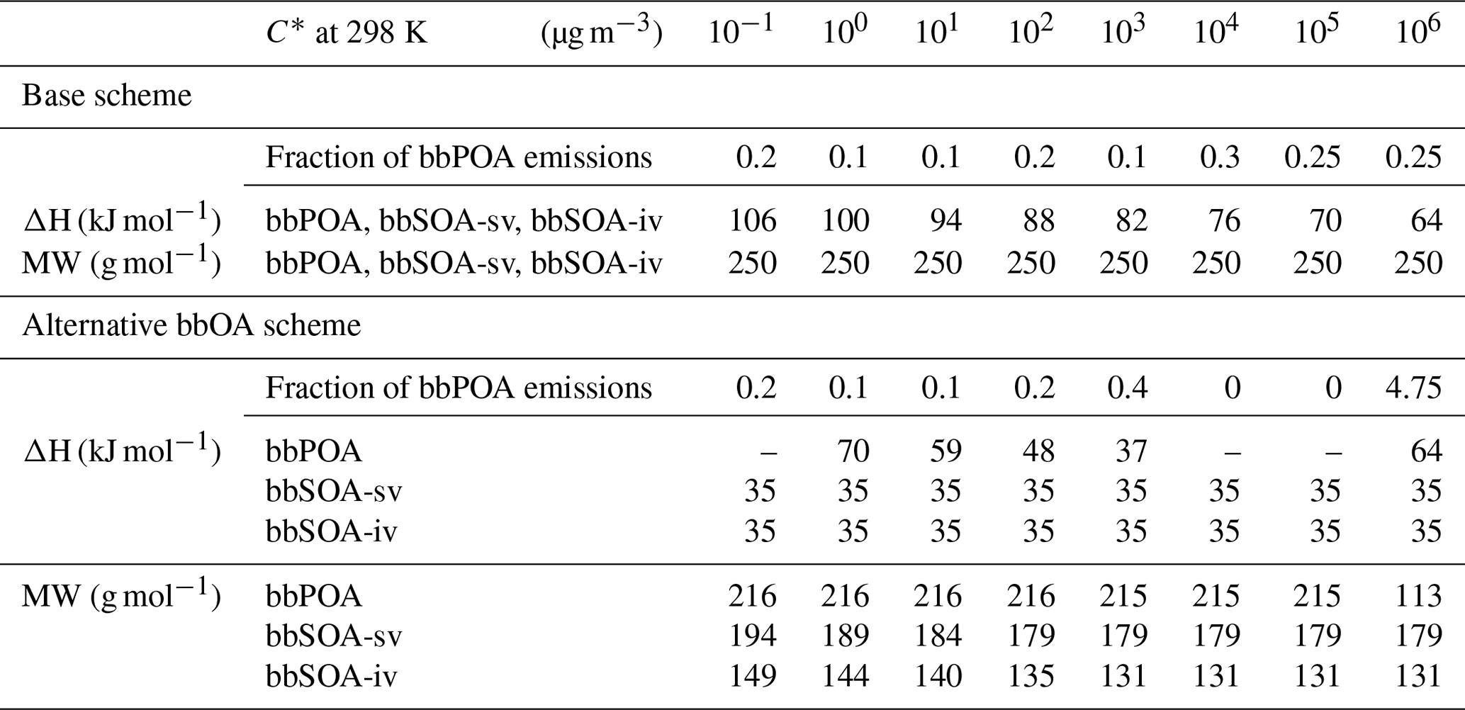
Table 1 summarizes the VBS parameters of all OA species in the base PMCAMx-SR simulation. The average molecular weight of all POA and bbPOA components is assumed to be 250 g mol⁻¹, that of aSOA components is assumed to be 150 g mol⁻¹, and that of bSOA species is assumed to be 180 g mol⁻¹. The effective enthalpies of vaporization of both POA and bbPOA species are based on fits of diesel and woodsmoke partitioning data (Lipsky and Robinson, 2006; Shrivastava et al., 2006).

Table 1 Parameters used to simulate bbPOA, bbSOA-sv, and bbSOA-iv in PMCAMx-SR.

2.2 Alternative bbOA scheme

The scheme of Ciarelli et al. (2017a, b) for the simulation of the emissions of organics from residential heating biomass burning and their evolution in the atmosphere during winter was also implemented in PMCAMx-SR. The organic PM emissions (assumed to be nonvolatile in the original inventory) are distributed in this scheme across five volatility bins with saturation concentrations values ranging from 10⁻¹ to 10³ µg m⁻³ following the volatility distribution and enthalpy of vaporization proposed by May et al. (2013). Organic vapors in this volatility range are assumed to react with OH forming semi-volatile oxidation products with an order-of-magnitude-lower volatility:

$$\begin{array}{}\text{(1)}& {\mathrm{bbPOG}}_i+\mathrm{OH}\to {\mathrm{bbSOG}}_{i-\mathrm{1}},\end{array}$$

where i is the corresponding volatility bin, bbPOG_i is the primary emissions in the gas phase, and bbSOG_i is their oxidation products. Fragmentation processes are implicitly assumed to balance the effect of the increase in oxygen content of the reacting molecules. Both schemes (base case and alternative) do not explicitly simulate the functionalization and fragmentation reactions. The alternative scheme of Ciarelli et al. (2017a, b) assumes that these two processes in a sense balance each other leading to a mass stoichiometric yield equal to unity in the corresponding net reaction.

All emitted IVOCs in this bbOA scheme are assumed to have a C^* value of 10⁶ µg m⁻³ (Ciarelli et al., 2017a, b), which is at the high end of the IVOC saturation concentration range. The emission rate of these IVOCs is assumed to be 4.75 times the primary OA emissions in the original inventory. The IVOCs are assumed to react according to the following reaction:

$$\begin{array}{}\text{(2)}& \begin{array}{rl}{\mathrm{bbPOG}}_{{\mathrm{10}}^{\mathrm{6}}}& +\mathrm{OH}\to \mathrm{0.143}{\mathrm{bbSOG}}_{{\mathrm{10}}^{\mathrm{3}}}+\mathrm{0.097}{\mathrm{bbSOG}}_{{\mathrm{10}}^{\mathrm{2}}}\\ & +\mathrm{0.069}{\mathrm{bbSOG}}_{{\mathrm{10}}^{\mathrm{1}}}+\mathrm{0.011}{\mathrm{bbSOG}}_{{\mathrm{10}}^{\mathrm{0}}},\end{array}\end{array}$$

yielding secondary products with saturation concentration ranging from $C^{*}=\mathrm{1}$ to 10³ µg m⁻³. In this reaction ${\mathrm{bbPOG}}_{{\mathrm{10}}^{\mathrm{6}}}$ stands for the primary emissions in the volatility bin with a C^∗ value equal to 10⁶µg m⁻³, whereas ${\mathrm{bbSOG}}_{{\mathrm{10}}^{\mathrm{3}}}$ to ${\mathrm{bbSOG}}_{{\mathrm{10}}^{\mathrm{0}}}$ are the secondary gas-phase oxidation products of the IVOCs with C^∗ values ranging from 10³ to 10⁰ µg m⁻³. For both primary and secondary compounds, aging is simulated assuming a gas-phase reaction rate constant with OH of 4 × 10⁻¹¹ cm³ molec.⁻¹ s⁻¹. The lowest volatility secondary bbPOA components in this scheme have $C^{*}={\mathrm{10}}^{-\mathrm{1}}$ µg m⁻³ since the $C^{*}=\mathrm{1}$ µg m⁻³ species can react with OH to form lower-volatility products.

Table 1 also summarizes the volatility distribution, the molecular weights, and the enthalpies of vaporization of all bbOA species used in the alternative bbOA modeling scheme in this study. The enthalpies of vaporization used in this bbOA scheme are the ones proposed in Ciarelli et al. (2017a, b). The structure of the VBS combined with the modular structure of PMCAMx-SR allows the user to change the corresponding parameters easily (volatility distributions, enthalpies of vaporization, aging scheme, etc.) and therefore change the OA parameterization for the source of interest.

3 Model application

In this study PMCAMx-SR is used to simulate three seasonally representative months (April, July, and September) during 2008 for the continental US. The modeling domain also included southern Canada and northern Mexico. The first 2 d of each simulation were excluded from our analysis to allow for model spin-up, but the corresponding results are shown in time series plots. The modeling domain covers a region of 5328 × 4032 km² with 36 × 36 km grid cell resolution and 25 vertical layers extending up to 19 km (Fig. 1). An annual CAMx simulation was performed for the same domain to obtain the necessary initial conditions used in our simulations for each month (ENVIRON, 2013).

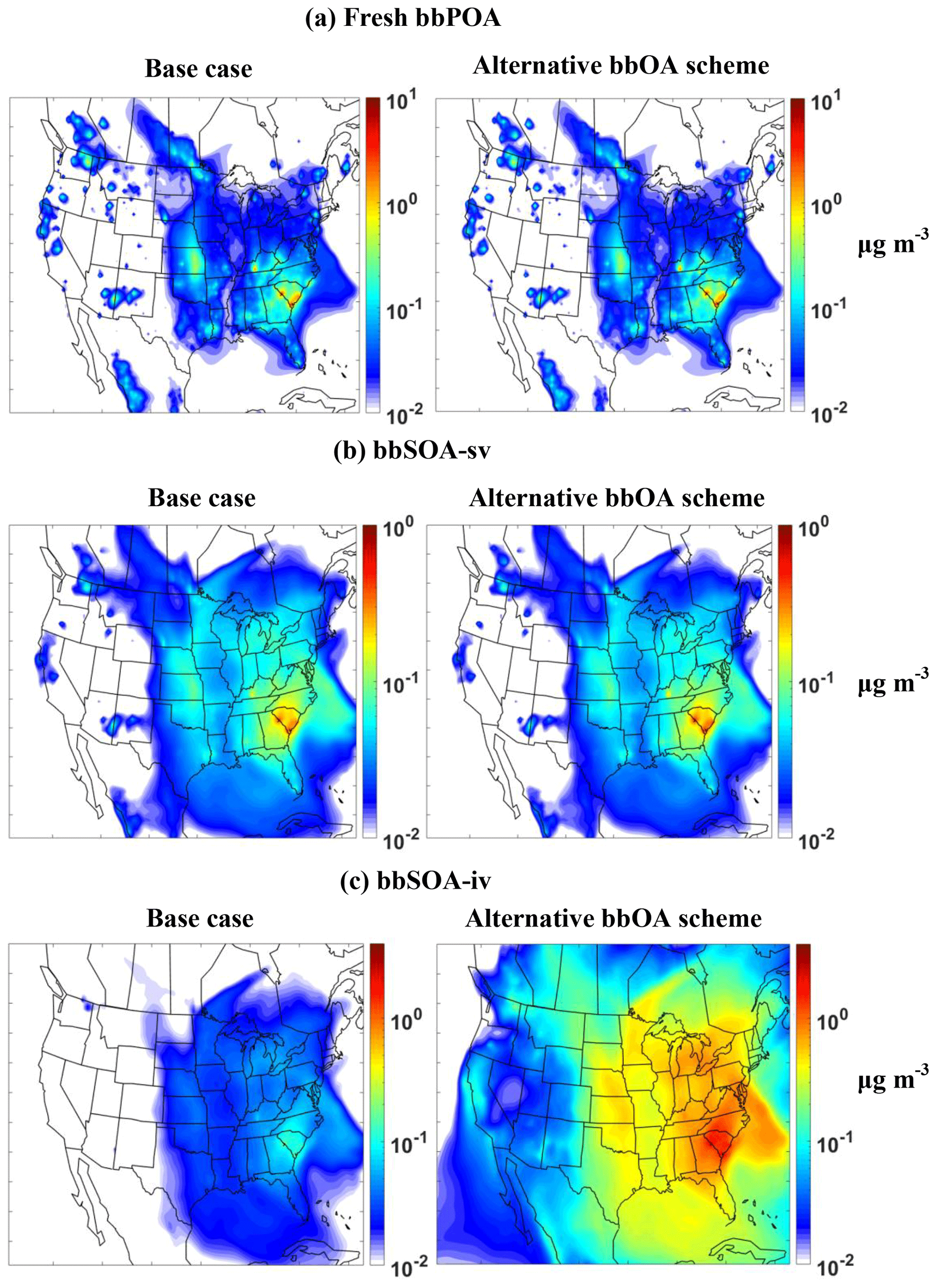
Figure 1 PMCAMx-SR-predicted ground-level concentrations of (a) fresh bbPOA, (b) SV-bbSOA-sv, and (c) SV-bbSOA-iv from all biomass burning sources during April 2008. Left column refers to the base case simulations and right column to the simulations with the alternative bbOA scheme. All concentrations are in µg m⁻³.

The Weather Research and Forecast Model (WRF) version 3.3.1 (NCAR, 2012) was used to produce the meteorological inputs needed by PMCAMx-SR. The land-use data were based on the U.S. Geological Survey Geographic Information Retrieval and Analysis System (USGS GIRAS) database. The photolysis rate input data were produced by the NCAR Tropospheric Ultraviolet and Visible (TUV) radiation model. The chemical boundary conditions were based on simulations using the MOZART global CTM (Emmons et al., 2010). Additional details about the model inputs can be found in Posner et al. (2019) and Theodoritsi et al. (2020b).

The emission inventory used in the current study tracks separately the biomass burning emissions from the emissions from other sources. The latter are based on the US National Emissions Inventory (NEI TSD, 2008). Biomass burning emissions include emissions of prescribed burning, agricultural burning, and wildfires, and the methods used for their estimation inventory be found in WRAP (2013). The fire activity data used are described in Ruminski et al. (2006), Eidenshink et al. (2007), and Mavko and Randall (2008). The approach used for the preparation, processing, and validation of fire activity data were similar to those of Wiedinmyer et al. (2006) and Raffuse et al. (2009). For fire consumption estimates CONSUME3 (Joint Fire Science Program, 2009) was used for all biomass burning sources except agricultural burns for which the method from the WRAP 2002 emissions inventory was employed (WRAP, 2005).

During all three examined periods, based on the emissions inventories used biomass burning was a significant POA source mainly in the southeast US (Posner et al., 2019; Theodoritsi et al., 2020b). Specifically, during April, July, and September, respectively, this source represents approximately 25 %, 65 %, and 37 % of the total POA emissions. During April 19 % of the domain-averaged bbPOA emissions rate is due to agricultural burning, 47 % to prescribed burning, and 34 % to wildfires. During July, due to the very high wildfire emissions mainly in northern California, the domain-averaged bbPOA emissions are mostly (96 %) due to this source. Agricultural burning contributed 1 % and prescribed burning the remaining 3 %. For September, wildfires in the west were still the dominant source, and they were responsible for 73 % of the domain bbPOA emissions. Prescribed burning was a significant source (22 % of the bbPOA emission), while agricultural burning was responsible for 5 % of the emissions. Posner et al. (2019) and Theodoritsi et al. (2020b) have presented analyses of the spatial distribution and magnitude of these bbPOA emissions.

4 Predicted bbOA concentrations

In this section the predictions of PMCAMx-SR for the base case and the alternative bbOA scheme are analyzed. In this work bbOA is defined as the sum of primary (bbPOA) and secondary (bbSOA) OA. The latter is the sum of bbSOA originating from semi-volatile organic compounds (bbSOA-sv) and from IVOCs (bbSOA-iv). The small SOA contribution from VOCs (Posner et al., 2019) is not explicitly accounted in the bbSOA but is included in the aSOA and bSOA simulated by the model. The results of the PMCAMx-SR simulations with the two schemes are shown in Figs. 1–3.

During April both schemes predict approximately the same bbPOA concentrations (Fig. 1) that were as high as 3.5 µg m⁻³ on a monthly average basis in the southeastern US. These high levels were mainly due to prescribed burning. The differences in predicted bbPOA levels by the two models were less than 0.1 µg m⁻³ (maximum difference in average levels) in all areas of the domain (Fig. 4) something expected given that they use the same volatility distributions for the primary LVOCs and SVOCs. Predicted average ground bbPOA levels over the US were approximately 0.02 µg m⁻³ (average of ground concentrations over the whole domain). The domain and simulation average bbPOA values are quite low given that fires often have a significant effect for only a few days for a limited area. These values are provided here mainly to facilitate the comparison of the two parameterizations. The predicted bbSOA-sv concentration fields were also quite similar (differences of less than 0.1 µg m⁻³) for the two schemes (Fig. 1). This is also the consequence of the similarity of the volatility distributions and chemical aging parameterizations used by the two schemes in the SVOC volatility range of the biomass burning emissions. While the average bbSOA-sv levels over the domain were quite similar to those of the bbPOA (around 0.02 µg m⁻³), the peak levels were lower with a maximum monthly average concentration of 0.5 µg m⁻³. This spreading of the bbSOA-sv further from the fires is the result of the time needed for the corresponding reactions to take place. The predictions of the two schemes are quite different though for bbSOA-iv (Fig. 1). For the base scheme, the bbSOA-iv is as important as the bbPOA and the bbSOA-iv contributes on average 0.02 µg m⁻³ of OA over the domain. The peak monthly average bbSOA-iv concentration is predicted to be approximately 0.2 µg m⁻³ in the southeast. The predictions for bbSOA-iv for the alternative scheme are approximately an order of magnitude higher, with a maximum average of 2 µg m⁻³ and a domain average of 0.2 µg m⁻³ (Fig. 1). Even if the IVOC emissions are assumed to be more volatile in the alternative scheme, their high emission rate allows the production of significant concentrations of secondary OA from biomass burning that extend over the eastern half of the country during this photochemically active period.

Both models predict that during April the bbSOA is the dominant component of bbOA on average over the domain, and even if it peaks in South Carolina with high levels in North Carolina and Georgia, it has average concentrations above 0.1 µg m⁻³ in most areas of the eastern US (Fig. 5a). The alternative scheme predicts that this bbSOA contribution is a factor of 5–10 higher and around or above 1 µg m⁻³ in the eastern US. Adding everything together the alternative scheme predicts an average bbOA concentration of 0.3 µg m⁻³ that is a factor of 5 higher than the average predicted by the base scheme (Fig. 6a).

During July, several major wildfires occurred in California, and consequently bbOA levels were particularly high in the western US (Fig. 2a) reaching levels around 100 µg m⁻³. This presents a very different situation compared to the spring month discussed above. Once more, the predictions of the two schemes for bbPOA were quite similar (differences of less than 20 %), even if the concentration levels at least in California were much higher. Despite the intensity of the fires in California, the low emissions in the rest of the country resulted in similar average bbPOA levels over the domain as in April (0.15 µg m⁻³) for both schemes. Both schemes predicted similarly high bbSOA-sv levels with monthly average values of up to 15 µg m⁻³ and domain average values of 0.2 µg m⁻³ (Fig. 2b). The alternative aging scheme predicts high bbSOA-iv that dominates the overall bbOA in the domain with an average of 2 µg m⁻³. The average bbSOA-iv but also the peak levels predicted by the base scheme are more than an order of magnitude lower (Fig. 2c). The average bbSOA predicted by the base scheme was approximately a factor of 7 lower (0.3 versus 2 µg m⁻³) for the domain (Fig. 5), while the total bbOA was a factor of 5 lower (Fig. 6). The differences between the two schemes exceeded 10 µg m⁻³ on a monthly average basis over California and were above 1 µg m⁻³ over a large part of the western US (Fig. S1).

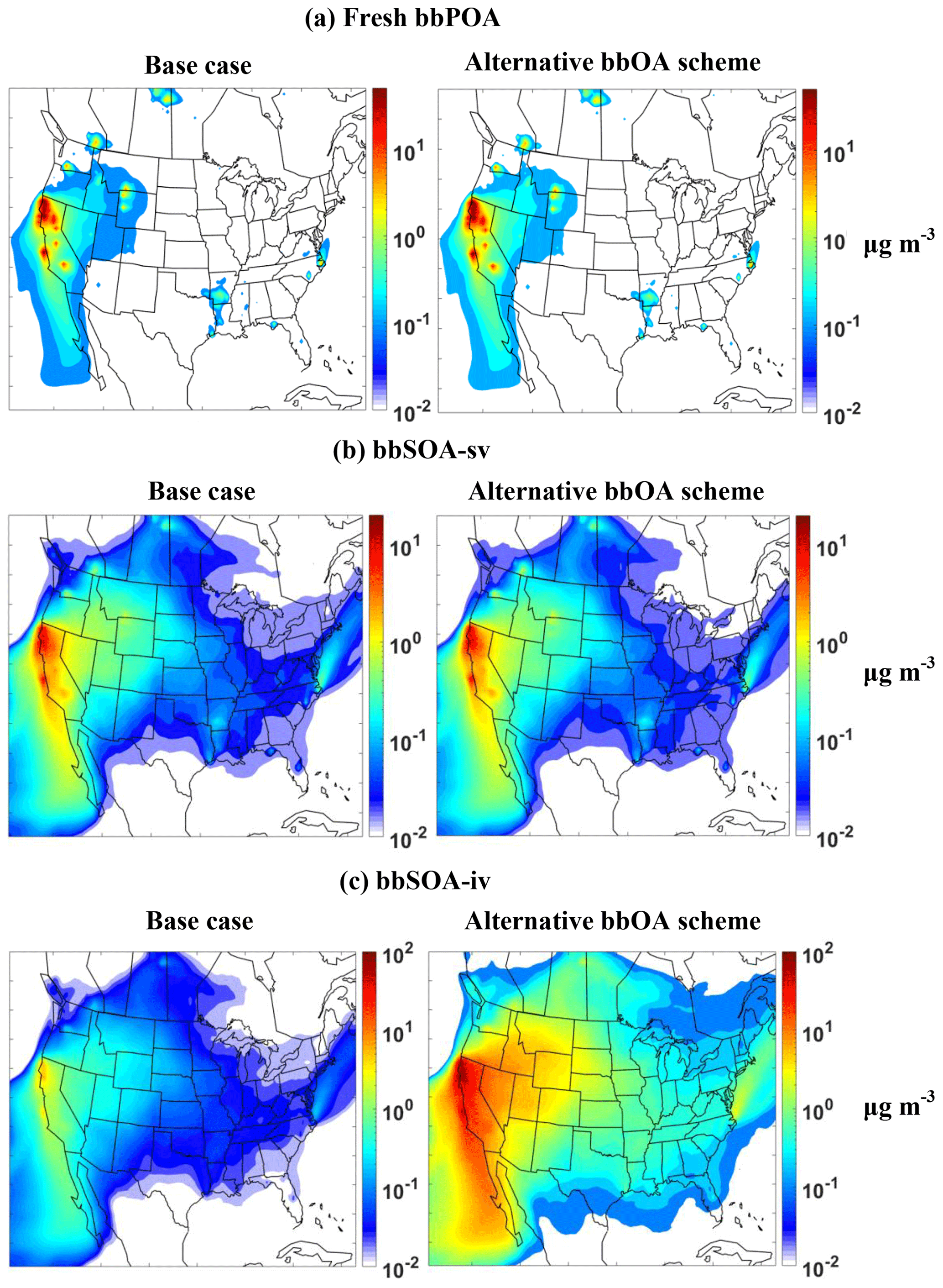
Figure 2 PMCAMx-SR-predicted ground-level concentrations of (a) fresh bbPOA, (b) SV-bbSOA-sv, and (c) SV-bbSOA-iv from all biomass burning sources during July 2008. Left column refers to the base case simulations and right column to the simulations with the alternative bbOA scheme. All concentrations are in µg m⁻³.

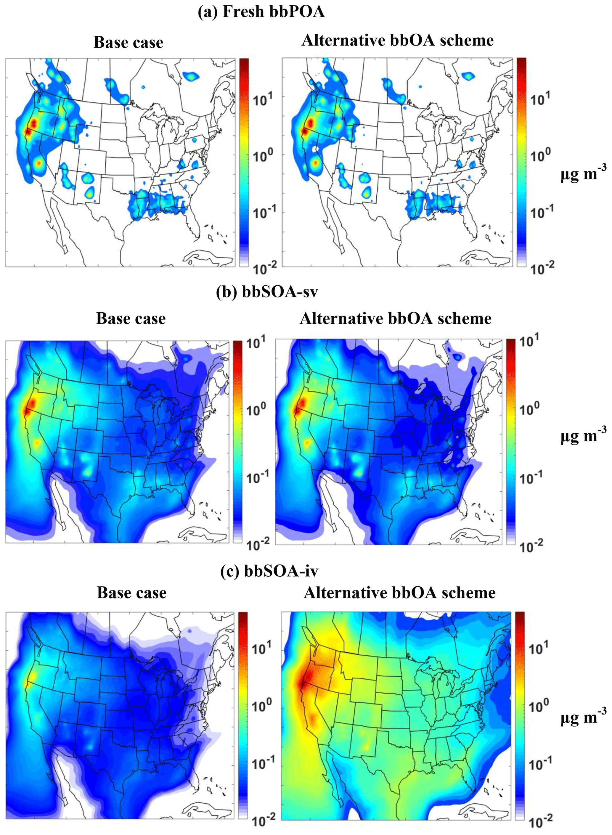
Figure 3 PMCAMx-SR-predicted ground-level concentrations of (a) fresh bbPOA, (b) SV-bbSOA-sv, and (c) SV-bbSOA-iv from all biomass burning sources during September 2008. Left column refers to the base case simulations and right column to the simulations with the alternative bbOA scheme. All concentrations are in µg m⁻³.

During September there were major wildfires once more in California but also in Oregon (Fig. 3). Smaller fires were present in New Mexico and in several southeastern states. The predicted bbPOA average concentration, similar for both schemes, were the lowest of the three simulated periods with a value of approximately 0.1 µg m⁻³. The local monthly maxima were 65 and 75 µg m⁻³ for the base case and the alternative aging scheme, respectively (Fig. 3a). The average bbSOA-sv concentration based on the predictions of both schemes was a factor of 6 higher (around 0.6 µg m⁻³) than the average bbPOA concentration. The average bbSOA-sv during the month exceeded 0.1 µg m⁻³ over a wide region covering most of the western coast of the US and parts of the Pacific. The peak monthly average bbSOA-sv concentration was 7 µg m⁻³ for both simulations. Finally, for the bbSOA-iv the alternative scheme predicted both domain average and peak concentrations that were approximately an order of magnitude higher than the base scheme (Fig. 3c). For the base case simulation, bbSOA-iv was as high as 4 µg m⁻³ with a monthly average value of approximately 0.05 µg m⁻³, whereas the same values for the alternative aging scheme were 45 and 0.7 µg m⁻³, respectively. As a result, the alternative scheme predicts average bbSOA levels that are a factor of 7 higher than the base case (0.1 versus 0.7 µg m⁻³) (Fig. 5c) and total bbOA levels that are a factor of 4 higher (Fig. 6c). For the peak monthly average concentrations, the differences are a factor of 5 for bbSOA and a factor of 1.5 for bbOA (given that the bbPOA is a dominant component near the fires).

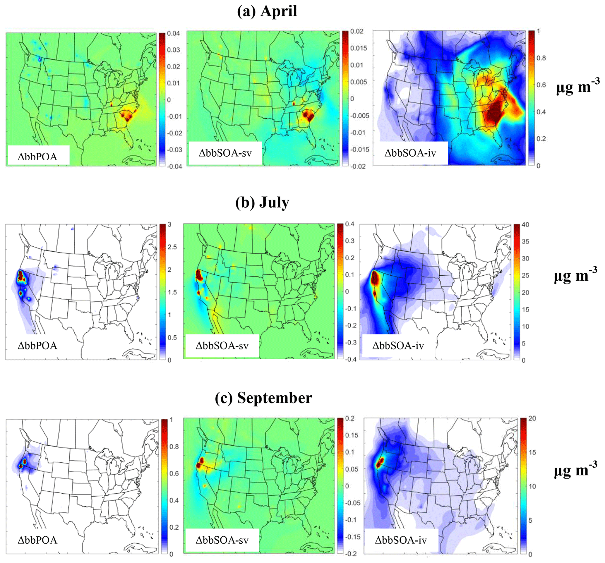
Figure 4 Average predicted absolute (µg m⁻³) difference (alternative aging scheme minus base case) of ground-level PM_2.5 bbPOA, bbSOA-sv, and bbSOA-iv concentrations from PMCAMx-SR base case and alternative aging scheme simulations during the modeled periods. Positive values indicate that the PMCAMx-SR alternative aging scheme simulations predicts higher concentrations.

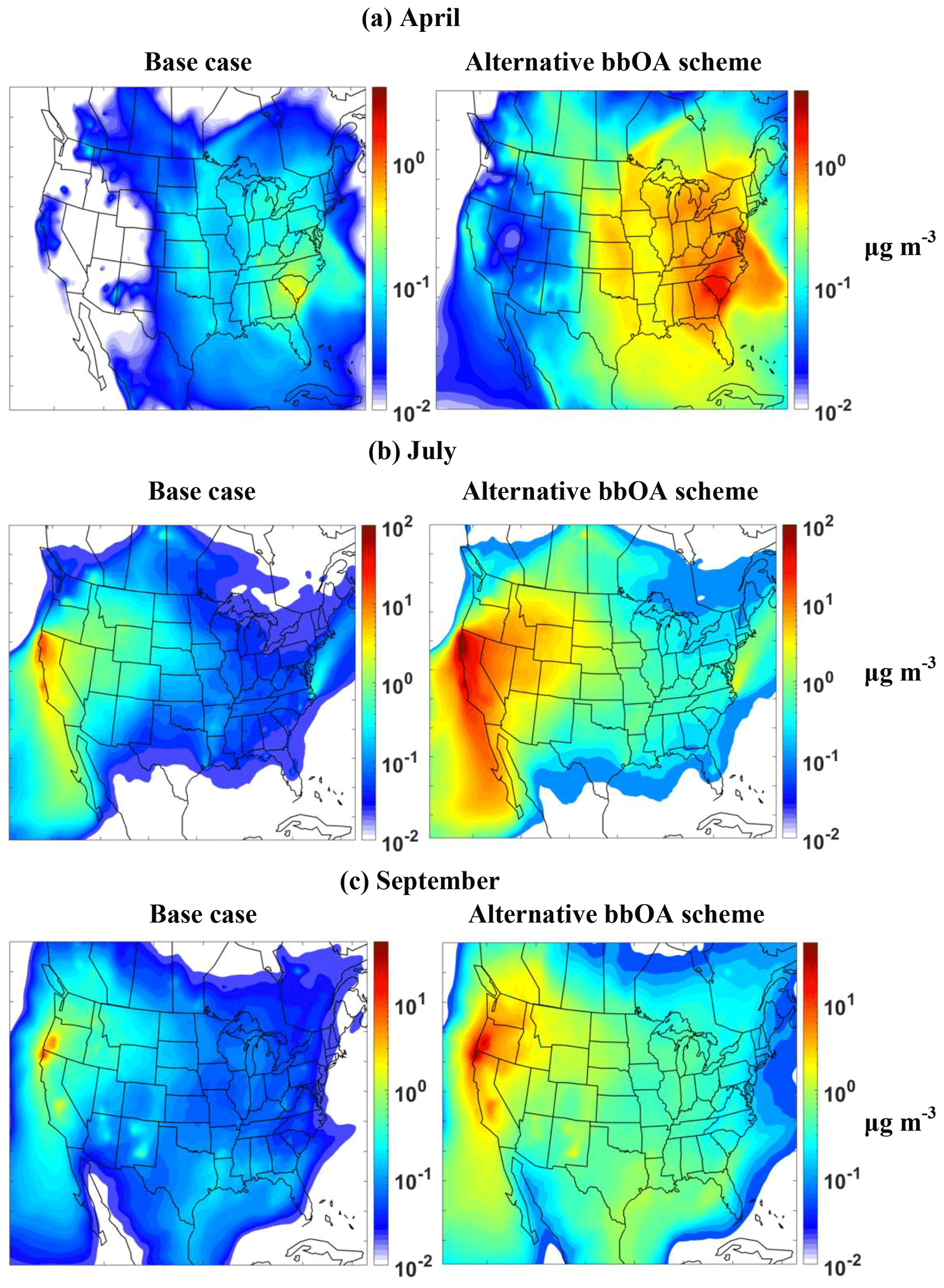
Figure 5 PMCAMx-SR-predicted ground-level concentrations of bbSOA-sv and bbSOA-iv from all biomass burning sources during (a) April, (b) July, and (c) September 2008. Left column refers to the base case simulations and right column to the simulations with the alternative bbOA scheme. All concentrations are in µg m⁻³.

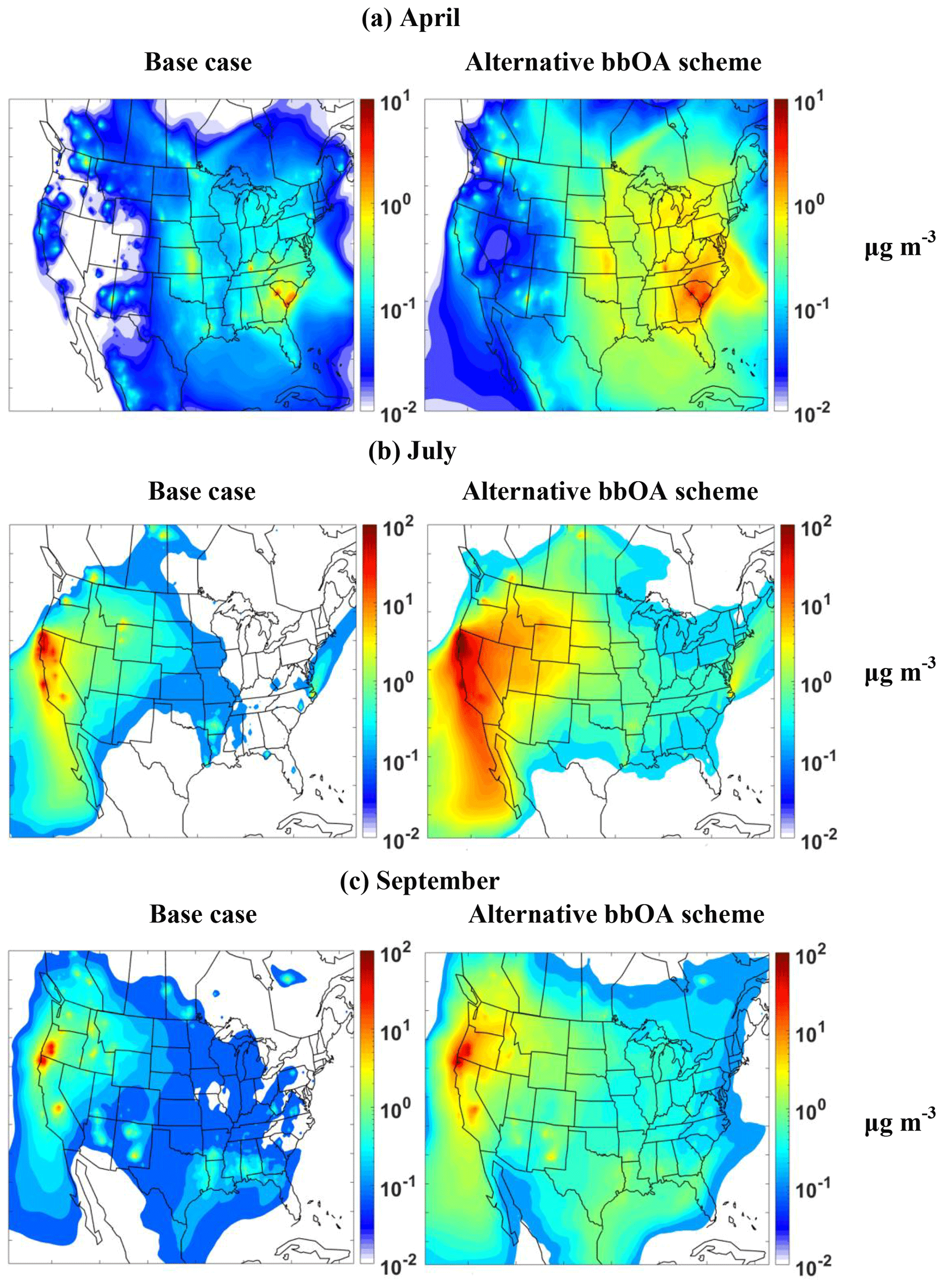
Figure 6 PMCAMx-SR-predicted ground-level concentrations of bbOA from all biomass burning sources during (a) April, (b) July, and (c) September 2008. Left column refers to the base case simulations and right column to the simulations with the alternative bbOA scheme. All concentrations are in µg m⁻³.

5 Model evaluation with field measurements

The predictions of PMCAMx-SR for daily average PM_2.5 OA were compared to the corresponding measurements in 161 Chemical Speciation Network (CSN) sites (located mainly in urban areas) and 162 Interagency Monitoring of Protected Visual Environments (IMPROVE) sites (located mostly in rural and remote areas). These daily average measurements were collected once every 3 or once every 6 d and include both the PM_2.5 mass concentration and its composition. The organic carbon (OC)/organic aerosol (OA) measurements are used here given our focus on biomass burning OA. The OC of PM_2.5 aerosol samples collected on quartz fiber filters is measured using thermal optical analysis with the corresponding temperature protocol (Chow et al., 2007). Most measurements were collected in periods during which the corresponding site was not impacted by biomass burning; therefore the use of the complete data set would complicate the interpretation of the evaluation results. To avoid this complication, we have followed Posner et al. (2019) and selected only the periods during which the base case of PMCAMx-SR predicts daily average concentrations higher than a threshold value. Three such thresholds were used to denote all periods with even a low biomass burning impact (threshold 0.1 µg m⁻³), all periods with intermediate or higher impact (threshold 0.5 µg m⁻³), and periods with high impact (threshold 1 µg m⁻³). The model prediction for the day and location of the measurement is compared directly to the corresponding measurement.

The statistical metrics that were used for the evaluation of the two schemes are the mean bias (MB), the mean absolute gross error (MAGE), the fractional bias (FBIAS), and the fractional error (FERROR) (Fountoukis et al., 2011):

$$\begin{array}{}\text{(3)}& {\displaystyle }\mathrm{MB}=\mathrm{1}/n{\sum }_{i=\mathrm{1}}^n(P_i-O_i),\text{(4)}& {\displaystyle }\mathrm{MAGE}=\mathrm{1}/n{\sum }_{i=\mathrm{1}}^n\left|P_i-O_i\right|,\text{(5)}& {\displaystyle }\mathrm{FBIAS}=\mathrm{2}/n{\sum }_{i=\mathrm{1}}^n(P_i-O_i)/(P_i+O_i),\text{(6)}& {\displaystyle }\mathrm{FERROR}=\mathrm{2}/n{\sum }_{i=\mathrm{1}}^n\left|P_i-O_i\right|/(P_i+O_i),\end{array}$$

where P_i is the predicted value of the pollutant concentration, O_i is the corresponding observed value, and n is the total number of data points used for the comparison.

Theodoritsi et al. (2020b) have already analyzed the performance of the base scheme of PMCAMx-SR for the same three periods. They concluded that during April the performance of the base scheme is good according to the Morris et al. (2005) criteria and the model tends to underpredict OA (fractional bias −0.16, fractional error 0.51 for the low threshold). PMCAMx-SR showed little bias (3 %–6 %) during July but had a relatively high fractional error (around 55 %), so its summer performance was considered average for the periods affected by biomass burning. Finally, the model overpredicted the OA levels in September with the errors increasing when the predicted bbOA concentration increased. This made its performance average to problematic during this period. The metrics of this evaluation by Theodoritsi et al. (2020b) for the base case PMCAMx-SR simulation can also be found in Table S1 for completeness.

The bbOA predictions of the alternative scheme are in general higher than those of the base scheme. This leads to a small improvement of the performance of PMCAMx-SR during April especially for the low bbOA threshold (Table 2). The model now tends to overpredict OA, while the base scheme underpredicted. For this case, the fractional bias is reduced (in absolute terms) from −0.16 to 0.11 and the fractional error from 0.51 to 0.48. The improvements are minor for the medium threshold, while for the high threshold the fractional bias increases (from −0.14 to 0.28) while the fractional error decreases (from 0.53 to 0.5). So overall, the use of the alternative scheme appears to lead to a small improvement of the PMCAMx-SR predictions during this period but with a tendency towards overprediction especially close to the sources of biomass burning.

Table 2 PMCAMx-SR alternative scheme OA prediction skill metrics against observed values from CSN and IMPROVE networks at biomass-impacted sites.

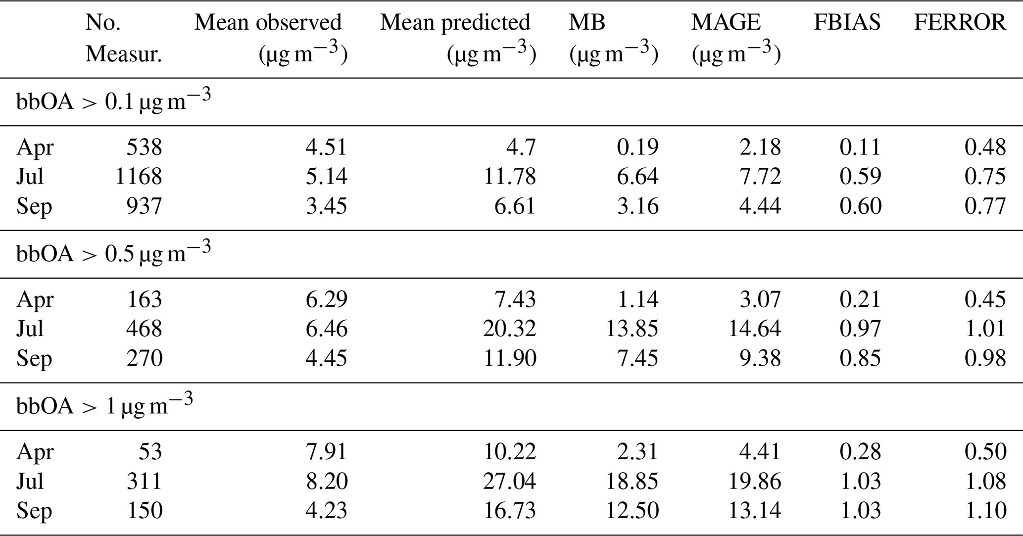
During July, the base scheme reproduced the OA observations in areas affected by biomass burning with little bias. The alternative scheme predicts a significantly higher SOA-iv production during this period and results in a substantial overprediction of the OA levels in areas with bbOA above all three thresholds (Table 2). The bias increases for the areas closer to the fires (higher threshold). These results strongly suggest that the alternative scheme is too aggressive in the production of SOA-iv during this summertime period with intensive wildfires.

PMCAMx-SR using the base scheme has difficulties reproducing the OA concentrations in areas affected by fires in the fall. Given that the base scheme already overpredicts OA levels, the increased SOA-iv predicted by the alternative scheme leads to additional deterioration of the model performance. The alternative scheme substantially overpredicts OA and the fractional bias increases closer to the sources of biomass burning. Overall, the performance of the alternative scheme during September is like that during July.

6 Importance of the VBS parameters used in the two bbOA schemes

The difference in the IVOC emissions and aging schemes appears to explain a large fraction of the differences in the predictions of the two schemes in the simulated periods. However, there are other potentially important differences in the parameters used in the two schemes. These different parameters include the enthalpy of vaporization and the molecular weights of the various bbOA components. The effect of these together with the effect of the assumed volatility distributions of the emitted bbOA components and the assumed aging schemes was investigated. Sensitivity tests were performed for one of the three periods (April 2008) to quantify the individual effect of these parameters on the predictions of PMCAMx-SR. The results of these tests and their comparison with the base case results are analyzed in the subsequent sections.

6.1 Enthalpy of vaporization

In this first sensitivity test, we changed the effective enthalpies of vaporization of the bbOA components (bbPOA, bbSOA-sv, bbSOA-iv) in the base scheme from their original values that varied from 64 to 106 kJ mol⁻¹ to those of the alternative scheme (Table 1). The new values were equal to 35 kJ mol⁻¹ for the bbSOA components and varied from 37 to 70 kJ mol⁻¹ for the bbPOA. This test allows us to quantify the importance of the significantly lower enthalpies used in the alternative scheme based on the work of Ciarelli et al. (2017a, b). All other parameters of the base scheme were kept the same.

The changes in the predictions of the model were small, a few percent or less (Fig. S2). The use of the higher original enthalpies of vaporization resulted in a little higher concentration for all bbOA components. The maximum monthly average changes were 0.3 µg m⁻³ for bbPOA, 0.03 µg m⁻³ for bbPOA-sv, 0.03 µg m⁻³ bbSOA-iv, and 0.4 µg m⁻³ for total bbOA all near Savannah, Georgia. However, for most of the US the change in total bbOA was less than 0.05 µg m⁻³. Therefore, the major differences in bbSOA-iv predictions of the base and alternative scheme were not due to their different enthalpies of vaporization.

6.2 Molecular weights

The base scheme assumes a molecular weight of 250 g mol⁻¹ for all bbOA components, while a range of molecular weights from 113 to 216 g mol⁻¹ is used in the alternative scheme (Table 1). These variable molecular weights are also intended to account for fragmentation effects and are accompanied by a stoichiometric coefficient equal to unity (instead of 1.075 in the base scheme). We replaced the molecular weights of the base scheme with those of the alternative, changed the stoichiometric coefficients in the aging reactions from 1.075 to 1, kept everything else the same, and repeated the April simulation.

The impact of these changes in the molecular weight values and stoichiometric coefficients was small (Fig. 7). The maximum concentration changes for the monthly average concentrations were 0.02 µg m⁻³ for bbPOA, 0.03 µg m⁻³ for bbSOA-sv, 0.1 µg m⁻³ for bbPOA-iv, and 0.1 µg m⁻³ for total bbOA all in the borders between South Carolina and Georgia. The use of the Ciarelli et al. (2017a, b) parameters (molecular weights and aging stoichiometric coefficients) led to very small reductions in the bbPOA and bbSOA-sv levels and small increases in the bbSOA-iv levels. The latter dominated the overall bbOA change which increased by 0.01 to 0.03 µg m⁻³ in large parts of the eastern US and by 0.03–0.1 µg m⁻³ in South Carolina and Georgia. These changes are still only a few percent. This small impact of the changes is partially due to the fact that they cancel each other to a large extent. The decrease in molecular weights leads to increased partitioning towards the particle phase and therefore higher bbOA levels, where the decrease in the aging stoichiometric coefficients has the opposite effect for the secondary components.

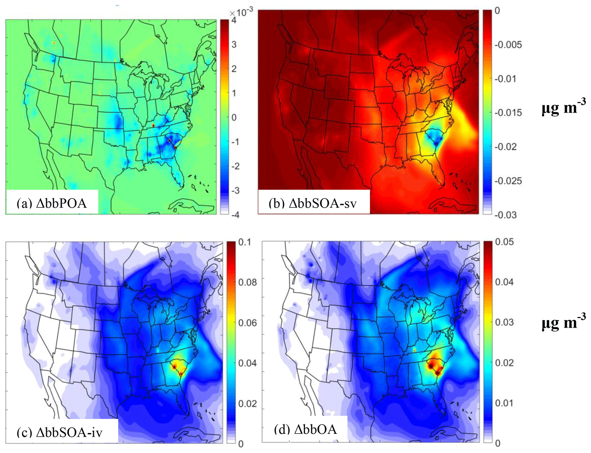
Figure 7 Average predicted increase (µg m⁻³) of the predictions of the base PMCAMx-SR scheme when the molecular weights and aging stoichiometric coefficient of Ciarelli et al., 2017a, b) are used compared to the predictions with the default values for ground-level PM_2.5 (a) bbPOA, (b) bbSOA-sv, (c) bbSOA-iv, and (d) bbOA during April 2008. Positive values indicate that the PMCAMx-SR base scheme with the molecular weights or stoichiometric coefficients of Ciarelli et al. (2017a, b) predicts higher concentrations.

6.3 Volatility distribution of biomass burning emissions

In this test, the emissions of the various organic compounds in the VBS from biomass burning were changed from these of the base scheme to those of Ciarelli et al. (2017a, b) (Table 1). This change does not affect the LVOC emissions and the SVOC emissions for C^* less or equal than 10² µg m⁻³. However, it increases the emissions of the 10³ µg m⁻³ volatility bin (by adding to these emissions those that are in the 10⁴ µg m⁻³ bin) and also significantly increases the emissions of the IVOCs in the 10⁶ µg m⁻³, while it zeros those in the 10⁵ µg m⁻³ bin.

The use of the Ciarelli et al. (2017a, b) volatility distributions leads to significant changes in the predicted bbOA concentration levels (Fig. 8). In all areas and for all bbOA components it predicts higher concentrations. The maximum concentration differences between the two simulations were 0.1 µg m⁻³ for bbPOA, 0.1 µg m⁻³ for bbSOA-sv, and 1.5 µg m⁻³ for bbSOA-iv. These differences are quite similar in magnitude to those of the base and alternative schemes (Fig. 4a). This strongly suggests that the differences in the assumed bbOA volatility-resolved emissions is mainly responsible for the differences in the bbOA predictions of the two schemes. For example, for the average total bbOA in the modeling domain the change in the volatility distributions led to an increase in the base case results of 0.14 µg m⁻³. This should be compared with 0.2 µg m⁻³, which is the difference between the average bbOA predicted by the base and alternative schemes.

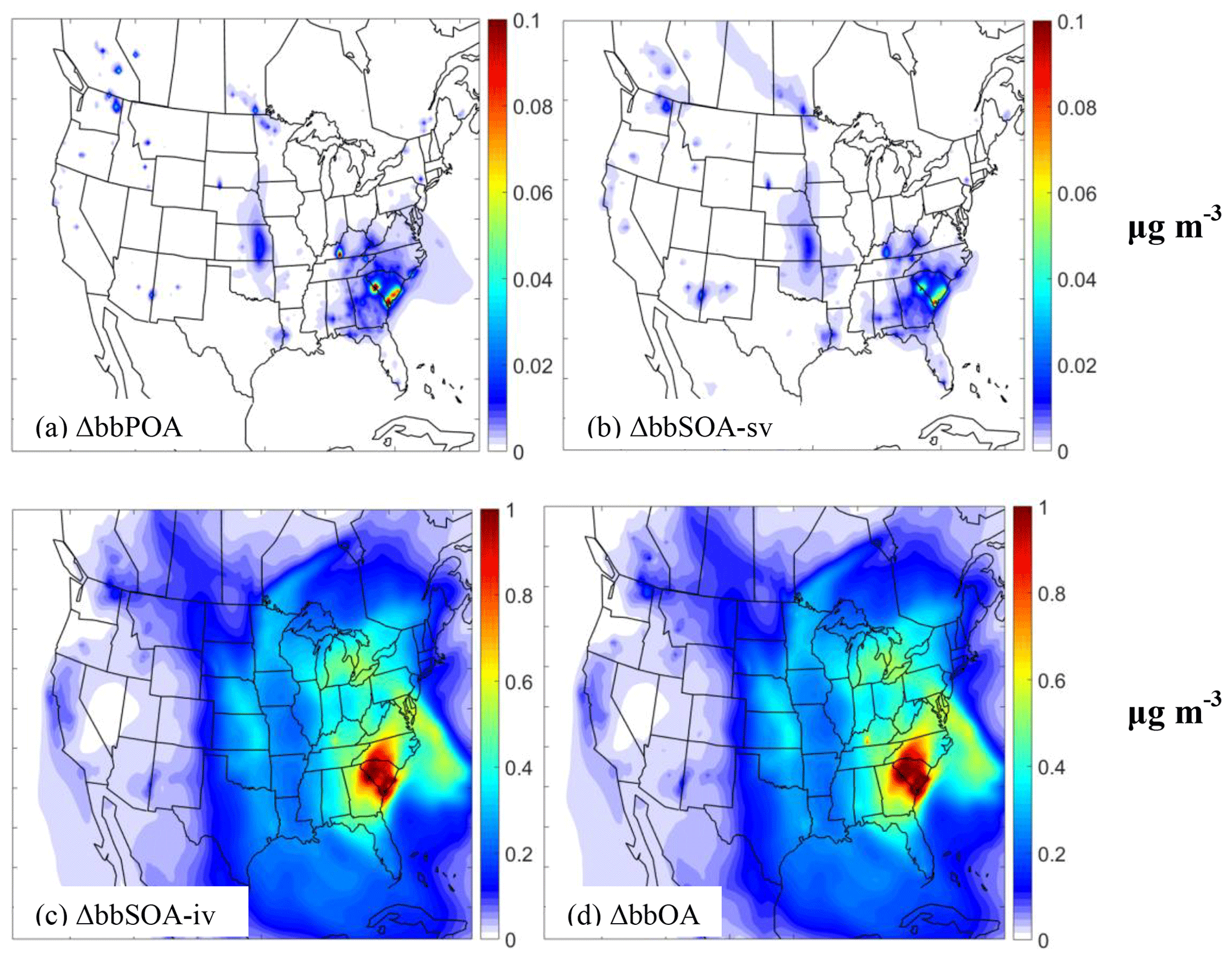
Figure 8 Average predicted increase (µg m⁻³) in the predictions of the base PMCAMx-SR scheme when the volatility distribution of Ciarelli et al. (2017a, b) is used for the biomass burning emissions compared to the predictions with the default values for ground-level PM_2.5 (a) bbPOA, (b) bbSOA-sv, (c) bbSOA-iv, and (d) bbOA during April 2008. Positive values indicate that the PMCAMx-SR base scheme with the volatility distribution of Ciarelli et al. (2017a, b) predicts higher concentrations.

The most important difference is the change in the IVOC emissions resulting in significant changes in the bbSOA-iv. The predicted bbSOA-iv of PMCAMx-SR with the base scheme using the default and the Ciarelli et al. (2017a, b) bbOA volatility distributions is depicted in Fig. 9. The monthly maximum concentration was predicted to be 0.2 and 1.5 µm m⁻³ for the base case and the alternative bbOA scheme, respectively, in South Carolina. This is also consistent, with our conclusion that the difference in the IVOC emissions is the leading cause of the differences in the predictions of the base and alternative schemes.

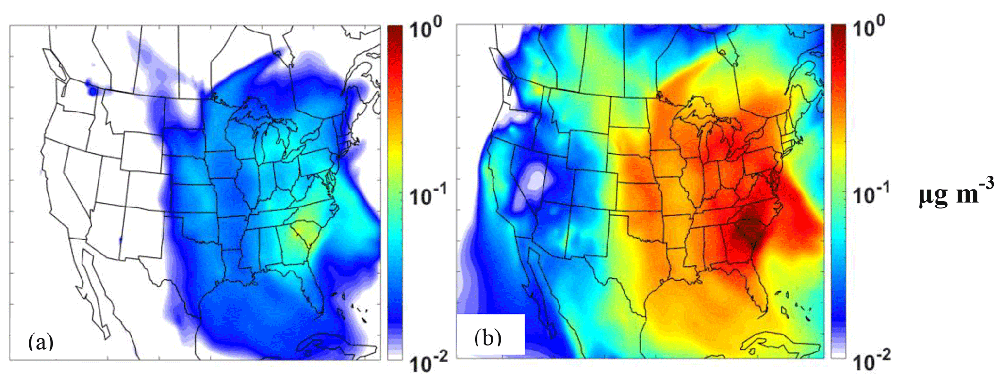
Figure 9 PMCAMx-SR-predicted ground-level concentrations (µg m⁻³) of bbSOA-iv for the base scheme using (a) the base case volatility distribution and (b) the Ciarelli et al. (2017a, b) volatility distribution.

7 Conclusions

An alternative bbOA scheme based on the work of Ciarelli et al. (2017a, b) has been used in PMCAMx-SR to quantify the impact of bbOA on ambient particulate-matter levels across the continental US during April, July, and September 2008. The alternative parameterization was originally developed based on residential heating biomass burning experiments (i.e., combustion in stoves). In this study we test its applicability for the simulation of the bbOA from other sources (wildfires, prescribed and agricultural burning) in different periods.

In general, the alternative scheme predicts much higher bbOA levels than the baseline scheme for all seasons. Both schemes suggest that secondary production is a major process for the average bbOA levels over the US in all examined periods. However, the alternative scheme predicts that the production of secondary aerosol from intermediate-volatility organic compounds emitted during biomass burning is a factor of 5–10 higher than that of the base scheme. The differences in the predictions of the other bbOA components (primary bbOA and bbOA from semi-volatile compounds) are low to modest.

A set of sensitivity tests showed that the most important difference between the two schemes is the assumed emission rate of intermediate-volatility organic compounds together with their oxidation to form secondary organic aerosol. The impact of other different parameters, including the assumed enthalpies of vaporization and molecular weights, was small.

The performance of PMCAMx-SR using the two schemes was evaluated against observed values obtained from 161 CSN and 162 IMPROVE network measurement sites across the US. During April the use of the alternative scheme leads to a small improvement of the performance of PMCAMx-SR. However, during the more photochemically active periods of July and September, with intense wildfires, the PMCAMx-SR performance for OA deteriorates when the alternative scheme is used instead of the base scheme. This strongly suggests that the production of SOA-iv under these conditions is too aggressive. Fragmentation reactions may become more important under these conditions leading to lower production of secondary organic aerosol. Our analysis suggests that the alternative scheme could be used during the spring-like conditions, but it should probably be avoided during summer-like periods characterized by intensive wildfire activities.

The alternative scheme considered here has been derived based on experiments using residential heating emissions. An assumption used in most biomass burning OA simulation efforts so far is that the same parameterization can be used for the different burning types: wildfires, agricultural burning, residential heating, prescribed burning, etc. Our work provides some support for the hypothesis that different parameterizations may be needed for residential heating and wildfires. This is clearly an issue that deserves additional attention in future modeling efforts.