the Creative Commons Attribution 4.0 License.
the Creative Commons Attribution 4.0 License.
 | 15 Mar 2021
Effects of spatial resolution on WRF v3.8.1 simulated meteorology over the central Himalaya
Jaydeep Singh
Narendra Ojha
Amit Sharma
Nadimpally Kiran Kumar
Kunjukrishnapillai Rajeev
Sachin S. Gunthe
V. Rao Kotamarthi
The sensitive ecosystem of the central Himalayan (CH) region, which is experiencing enhanced stress from anthropogenic forcing, requires adequate atmospheric observations and an improved representation of the Himalaya in the models. However, the accuracy of atmospheric models remains limited in this region due to highly complex mountainous topography. This article delineates the effects of spatial resolution on the modeled meteorology and dynamics over the CH by utilizing the Weather Research and Forecasting (WRF) model extensively evaluated against the Ganges Valley Aerosol Experiment (GVAX) observations during the summer monsoon. The WRF simulation is performed over a domain (d01) encompassing northern India at 15 km × 15 km resolution and two nests (d02 at 5 km × 5 km and d03 at 1 km × 1 km) centered over the CH, with boundary conditions from the respective parent domains. WRF simulations reveal higher variability in meteorology, e.g., relative humidity (RH = 70.3 %–96.1 %) and wind speed (WS = 1.1–4.2 m s−1), compared to the ERA-Interim reanalysis (RH = 80.0 %–85.0 %, WS = 1.2–2.3 m s−1) over northern India owing to the higher resolution. WRF-simulated temporal evolution of meteorological variables is found to agree with balloon-borne measurements, with stronger correlations aloft (r = 0.44–0.92) than those in the lower troposphere (r = 0.18–0.48). The model overestimates temperature (warm bias by 2.8 ∘C) and underestimates RH (dry bias by 6.4 %) at the surface in d01. Model results show a significant improvement in d03 (P = 827.6 hPa, T = 19.8 ∘C, RH = 92.3 %), closer to the GVAX observations (P = 801.4 hPa, T = 19.5 ∘C, RH = 94.7 %). Interpolating the output from the coarser domains (d01, d02) to the altitude of the station reduces the biases in pressure and temperature; however, it suppresses the diurnal variations, highlighting the importance of well-resolved terrain (d03). Temporal variations in near-surface P, T, and RH are also reproduced by WRF in d03 to an extent (r>0.5). A sensitivity simulation incorporating the feedback from the nested domain demonstrates the improvement in simulated P, T, and RH over the CH. Our study shows that the WRF model setup at finer spatial resolution can significantly reduce the biases in simulated meteorology, and such an improved representation of the CH can be adopted through domain feedback into regional-scale simulations. Interestingly, WRF simulates a dominant easterly wind component at 1 km × 1 km resolution (d03), which is missing in the coarse simulations; however, the frequency of southeasterlies remains underestimated. The model simulation implementing a high-resolution (3 s) topography input (SRTM) improved the prediction of wind directions; nevertheless, further improvements are required to better reproduce the observed local-scale dynamics over the CH.
- Article
(8925 KB) - Full-text XML
-
Supplement
(1302 KB) - BibTeX
- EndNote


The Himalayan region is one of the most complex and fragile geographical systems in the world, and it has paramount importance for climatic implications and air composition at the regional to global scales (e.g., Lawrence and Lelieveld, 2010; Pant et al., 2018; Lelieveld et al., 2018). The ground-based observations of meteorology and fine-scale dynamics are highly sparse and limited. In this direction, an intensive field campaign known as the Ganges Valley Aerosol Experiment (GVAX) (Kotamarthi, 2013) was carried out over a mountainous site in the central Himalaya, which provided valuable meteorological observations for atmospheric research, model evaluation, and further improvements. Accurate simulations of meteorology are needed for numerous investigations, such as to study the regional and global climate change, snow cover change, trapping and transport of regional pollution, and the hydrological cycle, especially the monsoon system (e.g., Sharma and Ganju, 2000; Bhutiyani et al., 2007; Pant et al., 2018). Studies focusing on this region have become more important due to increasing anthropogenic influences resulting in enhanced levels of short-lived climate-forcing pollutants (SLCPs) along the Himalayan foothills (e.g., Ojha et al., 2012; Sarangi et al., 2014; Rupakheti et al., 2017; Deep et al., 2019; Ojha et al., 2019). Although global climate models (GCMs) simulate the climate variabilities over the global scale, their application for reproducing observations in regions of complex landscapes is limited due to coarse horizontal resolution (e.g., Wilby et al., 1999; Boyle and Klein, 2010; Tselioudis et al., 2012; Pervez and Henebry, 2014; Meher et al., 2017). Mountain ridges, rapidly changing land cover, and low-altitude valleys often lie within a grid box of typical global climate models, resulting in significant biases in model results when compared with observations (e.g., Ojha et al., 2012; Tiwari et al., 2017; Pant et al., 2018). On the other hand, regional climate models (RCMs) at finer resolutions allow better representation of the topographical features, thus providing improved simulations of the atmospheric variability over regions of complex terrain. Several mesoscale models (e.g., Christensen et al., 1996; Caya and Laprise, 1999; Skamarock et al., 2008; Zadra et al., 2008) have been developed and successfully applied over different parts of the world. These studies have revealed that RCMs provide significantly new insights by parameterizing or explicitly simulating atmospheric processes over finer spatial scales. Nevertheless, large uncertainties are still seen over highly complex areas, indicating the effects of further unresolved terrain features (e.g., Wang et al., 2004; Laprise, 2008; Foley, 2010) and the need to improve the simulations.
Anthropogenic influences and climate forcing have been increasing over the Himalaya and its foothill regions since pre-industrial times (Bonasoni et al., 2012; Srivastava et al., 2014; Kumar et al., 2018). Consequently, an increase in the intensity and frequency of extreme weather events has been observed over the Himalayan region (e.g., Nandargi and Dhar, 2012; Sun et al., 2017; Dimri et al., 2017) in the past few decades. These events include extreme rainfall and resulting flash floods, cloudbursts, and landslides, and the associated weather systems range from mesoscale to synoptic-scale phenomena. Unfortunately, the lack of an observational network covering the Himalaya and foothills with sufficient spatiotemporal density inhibits the detailed understanding of the aforementioned processes as well as meteorological and dynamical conditions in the region. Therefore, the usage of regional models, evaluated against available in situ measurements, can fill the gap for investigating atmospheric variability in the observationally sparse and geographically complex mountain terrain of the Himalaya.
The biases in simulating the meteorological parameters, especially in the lower troposphere, are associated with several factors, e.g., representation of topography, land use, surface heat and moisture flux transport, and parameterization of physical processes (e.g., Lee et al., 1989; Hanna and Yang, 2001; Cheng and Steenburgh, 2005; Singh et al., 2016). The Weather Research and Forecasting (WRF) model has been used for experiments over complex terrain around the world, e.g., the Himalaya region (e.g., Sarangi et al., 2014; Singh et al., 2016; Mues et al., 2018; Potter et al., 2018; Norris et al., 2020; Wang et al., 2020), the Tibetan Plateau (e.g., Gao et al., 2015; Zhou et al., 2018), and multiple mountain ranges in the western United States (e.g., Zhang et al., 2013), to evaluate and study meteorology and dynamics. A cold bias was reported in this model over the Tibetan Plateau and the Himalayan region by Gao et al. (2015). The near-surface winds showed biases linked to unresolved processes in the model, such as sub-grid turbulence and land–surface atmospheric interactions, in addition to the boundary layer parametrization (Hanna and Yang, 2001; Zhang and Zheng, 2004; Cheng and Steenburgh, 2005). Zhou et al. (2018) found lower biases in simulated winds after considering the turbulent orographically formed drag over the Tibetan Plateau.
The WRF model, with suitably chosen schemes, has been shown to reproduce the regional-scale meteorology (Kumar et al., 2012) and to some extent also the mountain–valley wind systems (Sarangi et al., 2014) and boundary layer dynamics (Singh et al., 2016; Mues et al., 2018) over the Himalayan region. Nevertheless, local meteorology is still difficult to simulate accurately. Mues et al. (2018) performed a high-resolution WRF simulation over the Kathmandu valley of the Himalaya and reported overestimation of 2 m temperature and 10 m wind speed, which they attributed to insufficient resolution of the complex topography, even at a resolution of 3 km. Although few studies have used the WRF model at very high resolution over the Himalayan region (e.g., Cannon et al., 2017; Mues et al., 2018; Potter et al., 2018; Zhou et al., 2018, 2019; Norris et al., 2020; Wang et al., 2020), the model performance over complex terrains like the Himalaya still requires improvement, which can be achieved through an extensive evaluation at sub-kilometer resolution against an intensive field campaign. The main objectives of the study are as follows:
-
to examine the model performance over the CH at varying resolutions (15, 5 and 1 km) by evaluating several model diagnostics against the observations made during the GVAX campaign;
-
to investigate the effect of feedback from the nest to the parent domain, as this might allow configuring a model setup covering the larger Indian region with more accurate results over the Himalaya; and
-
downscaling to a sub-kilometer (333 m) resolution with the implementation of a very high-resolution (3 s) topographical input into the model to examine the potential of simulations in reproducing local-scale dynamics.
The subsequent section (Sect. 2) describes the model setup, followed by the experimental design and a discussion of datasets used for model evaluation. Section 3 provides a comparison of model results with the ERA-Interim reanalysis (Sect. 3.1), radiosonde observations (Sect. 3.2), and ground-based measurements (Sect. 3.3). Analysis of domain feedback is presented in Sect. 3.4, and the effect of implementing high-resolution topography is investigated in Sect. 3.5, followed by the summary and conclusions in Sect. 4.
2.1 Model setup and experimental design
The WRF model version 3.8.1 has been used in the present study. WRF is a mesoscale, non-hydrostatic, numerical weather prediction (NWP) model with advanced physics and numerical schemes for simulating meteorology and dynamics. WRF-ARW uses an Eulerian mass-based dynamical core with terrain-following vertical coordinates (Skamarock et al., 2008). ERA-Interim reanalysis from the European Centre for Medium-Range Weather Forecasts (ECMWF), available at a temporal resolution of 6 h and a horizontal resolution of with 37 vertical levels from the surface to the top at 1 hPa (Dee et al., 2011), has been used to provide the initial and lateral boundary conditions to the WRF model. Static geographical data from the Moderate Resolution Imaging Spectroradiometer (MODIS), available at 30 s horizontal resolution, are utilized for land use and land cover.
The Goddard scheme is used for shortwave radiation (Chou and Suarez, 1994), while longwave radiation is simulated by the rapid radiative transfer model scheme (Mlawer et al., 1997). For resolving the boundary layer processes the first-order Yonsei University (YSU) scheme based on non-local closure (Hong et al., 2006) is used, including an explicit entrainment layer with the K-profile in an unstable mixed layer. The planetary boundary layer (PBL) height is determined from the Richardson number (Rib) method in this PBL scheme. Convection is parameterized by the Kain–Fritsch (KF) cumulus parameterization (CP) scheme, accounting for sub-grid-level processes in the model such as precipitation, latent heat release, and the vertical redistribution of heat and moisture as a result of convection (Kain, 2004). With the increase in model grid resolution to less than 10 km (known as “grey area”), the CP scheme is usually turned off, and cloud and precipitation processes are resolved by the microphysics (MP) scheme (Weisman et al., 1997). In the present study, the CP scheme is used for d01, while it is turned off for d02 and d03. The Thomson microphysics scheme containing prognostic equations for cloud water, rainwater, ice, snow, and graupel mixing ratios is used (Thompson et al., 2004). Parameterization of surface processes is done with the MM5 Monin–Obukhov scheme and unified Noah land surface model (LSM) (Chen and Dudhia, 2001; Ek et al., 2003; Tewari et al., 2004). The Noah LSM includes a single canopy layer and four soil layers at 0.1, 0.2, 0.6, and 1 m within 2 m of depth (Ek et al., 2003).
The model is configured with three domains of 15 km (d01), 5 km (d02), and 1 km (d03) horizontal grid spacing using Mercator projection centering at Manora Peak (79.46∘ N, 29.36∘ E; ∼ 1936 m a.m.s.l.) in the central Himalaya. The topography within the model domains is highly complex, as evident from the ridges (Fig. 1). The outer domain d01 includes the northern part of the Thar Desert, part of Indo-Gangetic Plain (IGP), and the Himalayan mountains, while the innermost domain d03 consists of mostly mountainous terrain. The model has 51 atmospheric vertical levels with the top at 10 hPa. For d01, 100 east–west and 86 north–south grid points are used to account for the effect of synoptic-scale meteorology, e.g., the Indian summer monsoon. The d02 has 88 east–west and 76 north–south grid points covering a sufficient spatial region around the observational site to consider the effects of mesoscale dynamics, e.g., changes in wind pattern due to orography. The innermost domain, d03, has 126 east–west and 106 north–south grid points to resolve local effects, e.g., convection, advection, turbulence, and orthographic lifting.

Figure 1Topography represented in the WRF model domains (a) with three horizontal resolutions, namely domain d01 (15 × 15 km), domain d02 (5 × 5 km), and domain d03 (1 × 1 km). Each box inside a panel corresponds to the nested domain. The triangle in the innermost box indicates the location of the GVAX campaign site, i.e., Manora Peak in Nainital. The bottom panels (b, c, d) indicate the topography of each individual domain (left to right). The finest nest inside d03 (d) is d04 at the resolution of 333 m (discussed in Sect. 3.5).
For d01, boundary conditions are provided from the ERA-Interim reanalysis, as explained earlier. Model simulations have been performed for the 4 months of the summer monsoon: 1 June 2011 to 30 September 2011 (JJAS). This simulation period is chosen considering the availability of continuous observations from 11 June 2011 and to allow a sufficient spin-up time of 10 d for the model to achieve its equilibrium state (Angevine et al., 2014; Seck et al., 2015; Jerez et al., 2020). Only the outer domain d01 is nudged with the global reanalysis for temperature, water vapor, and the zonal and meridional (u and v) components of the wind using a nudging coefficient of 0.0006 (6 × 10⁻⁴) at all vertical levels (e.g., Kumar et al., 2012). Several of the configuration options, e.g., physics and meteorological nudging, are selected following earlier applications of this model over this region (e.g., Kumar et al., 2012; Ojha et al., 2016; Singh et al., 2016; Sharma et al., 2017).
2.2 Observational data
We utilize observations during an intensive field campaign – the Ganges Valleys Aerosol Experiment (GVAX) – to evaluate model simulations. The GVAX campaign was carried out using the Atmospheric Radiation Measurement (ARM) Climate Research Facility of the U.S. Department of Energy (DOE) from 10 June 2011 to 31 March 2012 at ARIES, Manora Peak in Nainital (e.g., Kotamarthi, 2013; Singh et al., 2016; Dumka et al., 2017). This observational site (79.46∘ N, 29.36∘ E; 1940 m above sea level) is located in the central Himalaya, as shown in Fig. 1. The surface-based meteorological measurements of ambient air temperature, pressure, relative humidity, precipitation, and wind (speed and direction) were made using an automatic weather station at 1 min temporal resolution. The instantaneous values of the observations are compared with hourly instantaneous model output at the nearest grid point.
The vertical profiles of temperature, pressure, relative humidity, and horizontal wind (speed and direction) were obtained by four launches (00:00, 06:00, 12:00, and 18:00 UTC) of the radiosonde each day during the campaign (Naja et al., 2016). The continuous vertical profiles of the meteorological parameters except wind speed and direction were available from the end of June 2011 through the entire study period, whereas valid and quality wind data were available only for September 2011. Hence, in this study, radiosonde measurements from 1 July 2011 onwards are used for the model evaluation of meteorological parameters, except wind speed and direction, which are evaluated only for September. A total of 309 valid profiles of temperature and relative humidity and 104 profiles of wind are used. Statistical metrics such as the mean bias (MB), root mean square error (RMSE), and correlation coefficient (r) are used for the model evaluation, and a description of these metrics is given in the Supplement.
3.1 Comparison with ERA-Interim reanalysis
Here, we have used the ERA-Interim data for comparison with WRF output. We first compare the WRF-simulated spatial distribution of meteorological parameters (surface pressure, 2 m air temperature, 2 m RH, and 10 m WS) with the ERA-Interim reanalysis over the common region of all the domains averaged for the entire simulation period (Fig. 2). The three contours of the topographic height of 500, 1500, and 2000 m are used to relate the meteorological features to the resolved topography in three domains. The common area in all domains includes the low-altitude IGP region in the south (elevation of less than 400 m; Fig. 1) and elevated mountains of the central Himalaya in the north. Also, for a consistent comparison, model-simulated values are taken at the same time intervals as in ERA-Interim data (i.e., every 6 h). From the comparison presented in Fig. 2, it is evident that the meteorological parameters simulated by the model are dependent on the model grid resolution. The existence of the sharp-gradient topographic height (SGTH) of about 1600 m from the foothill of the Himalaya to the observational site modifies the wind pattern and moisture content differently at different grid resolutions, indicating the critical role of mountain orography. The surface pressure explicitly depends upon the elevation of a location from mean sea level. The contour of the pressure parameter from ERA-Interim data shows the surface pressure of about 900 hPa for the observational site Manora Peak, and it varied from 550 to 975 hPa within this region, while WRF-simulated pressure is 869, 835, and 827 hPa for d01, d02, and d03, respectively. WRF-simulated surface pressure ranges from 821.9 hPa over the high-altitude CH region to 977.0 hPa in the IGP region within d01. Simultaneously, the range of variation in the surface pressure is 788.1–977.5 and 760.4–977.7 hPa within d02 and d03, respectively, and the minimum pressure decreases from d01 to d03, which is attributed to the improvement in resolved topography on increasing model grid resolution. However, the effects of the SGTH are not observed for temperature, wind, and RH in ERA-Interim contours due to the unresolved topographic features. Simulated maps show the spatial homogeneity of meteorological parameters over the flat terrain of IGP in the foothills of the Himalaya compared to the elevated central Himalayan region.

Figure 2Contours in the first three columns show WRF results for the three domains (first column: d01, second column: d02, third column: d03), and the fourth column shows corresponding parameters from the ERA-Interim reanalysis. The first row shows mean surface pressure during the monsoon (JJAS), the second row shows 2 m temperature (in ∘C), the third row shows 2 m relative humidity (RH; %), and the bottom row shows 10 m wind speed (WS; m s−1) along with three elevation contours at 500 m (dashed), 1500 m (thin solid), and 2000 m (thick solid).
The effect of spatial resolution is clearly observed over the mountainous region of the Himalaya, where the size of the mountains changes abruptly, with the modeled output showing increasingly distinct features with increasing grid resolution. On the other hand, there are minimal differences in the topography of the IGP, and hence the meteorological features associated with the topography are well captured in the model even at a coarser resolution of 15 km.
Model simulations show the topography-dependent spatial variation in 2 m temperature in the ranges of 20.0–29.5 ∘C in d01,17.3–29.6 ∘C in d02, and 15.5.0–29.9 ∘C in d03, with the lowest values simulated over the elevated mountain peaks and higher values over the temperate IGP region. The contours in three model domains show an explicit dependency of 2 m temperature on the grid resolution over the mountainous region. With increasing model resolution, the topography is resolved to a greater extent, and lower temperature is simulated at higher surface elevations, as expected. Further, the estimation of water vapor is essentially needed for both climate and numerical weather prediction (NWP) applications. Figure 2 shows that the simulated relative humidity is above 70 % in all three domains for the monsoon season. The variations (minimum–maximum) in the relative humidity in the ERA-Interim (80 %–85 %) dataset over the domains d01 (77 %–93 %), d02 (74 %–95 %), and d03 (70 %–96 %) are generally comparable. The mountain slopes provide uplift to the moist monsoonal air that on ascent subsequently saturates and increases the relative humidity to about 90 % as observed over the grid encompassing the site. Contour lines (1500 and 2000 m in Fig. 2) depict the low pressure and temperature with the higher relative humidity feature of the peaks, and these features are sharper as the resolution increases from d01 to d03.
The wind speed is highly dependent upon the model grid resolution and orography-induced circulations during different seasons (Solanki et al., 2016, 2019), and this is reflected in Fig. 2. As mentioned earlier, although the topography of the IGP region does not vary abruptly, the magnitude of the wind speed over this region and over the complex Himalayan region is found to change significantly at different model resolutions, thereby indicating that the wind speed is very sensitive to both model resolution and topography. The wind speed in d01 varies from 1.3 to 2.8 m s−1, while the wind variations in domains d02 (1.2–3.4 m s−1) and d03 (1.3–4.2 m s−1) show higher variability than that in ERA-Interim (1.2–2.3 m s−1) due to finer resolution of the WRF. Overall, the impact of the topography resolved at higher resolution in WRF shows the contrasting differences in surface pressure, temperature, relative humidity, and wind speed compared to the coarse-resolution ERA-Interim dataset.
3.2 Comparison with radiosonde observations
The intensive radiosonde observations made during the GVAX field campaign at Manora Peak (79.46∘ N, 29.36∘ E; ∼ 1936 m a.m.s.l.) in the central Himalaya (shown in Fig. 1) are used for the evaluation of model resolutions. The comparison of the model-simulated profiles of temperature, relative humidity, and wind speed against the radiosonde observations is shown in Fig. 3.
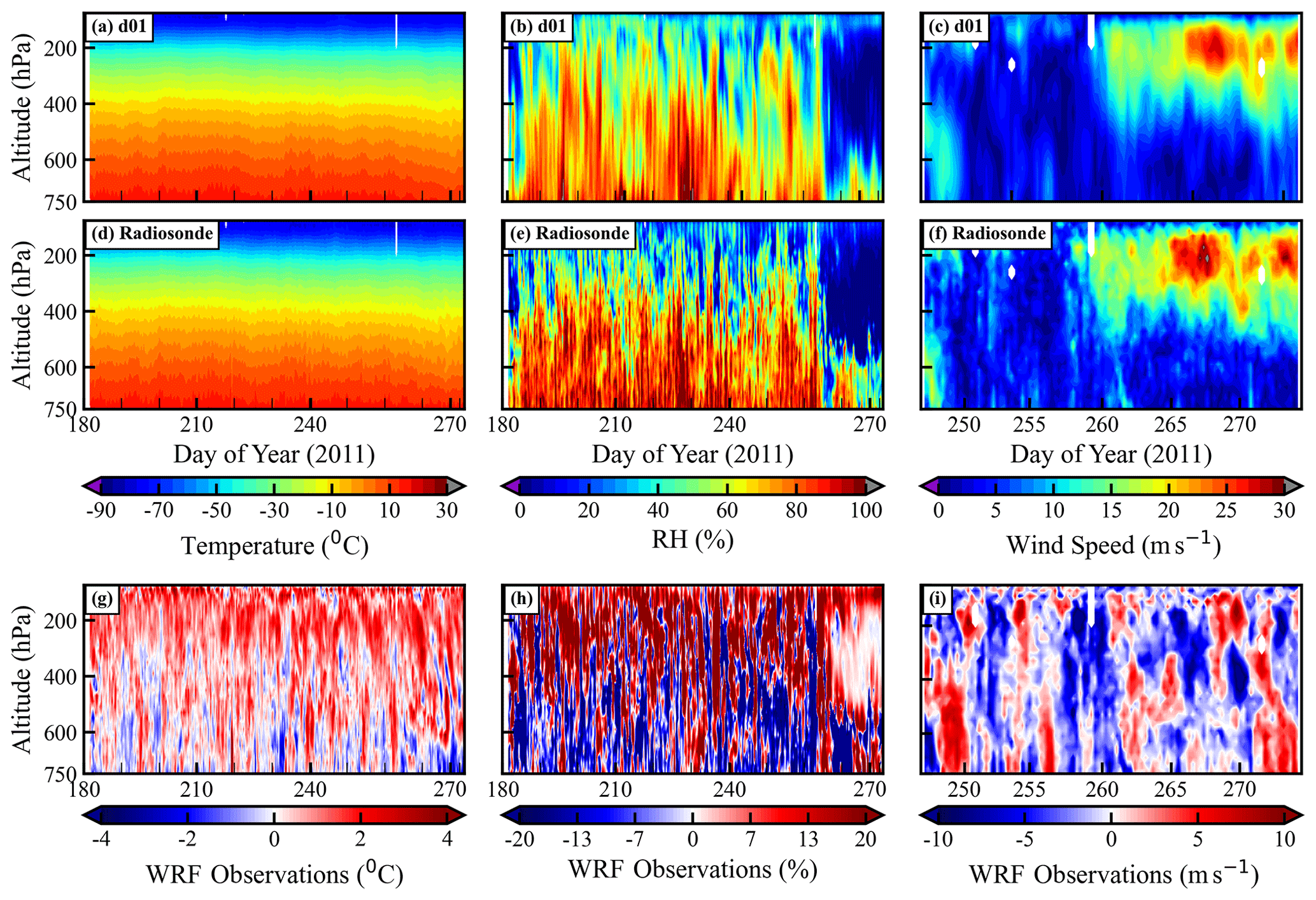
Figure 3The comparison of simulated vertical profiles of (a) temperature (∘C), (b) relative humidity (RH; %), and (c) wind speed (m s−1) in d01 with the radiosonde observations (d, e, f). The x axis in (a), (b), (d), (e), (g), and (h) shows the day of the year in 2011 starting from 1 July (182nd day) to 30 September (273rd day). The vertical profiles of wind speed (c, f) are plotted only for September 2011. The third row (g, h, i) shows the difference in temperature, relative humidity, and wind speed between the WRF d01 simulation and radiosonde observations.
The inversion of temperature at the top of the troposphere occurred at ∼ 90 hPa (∼ 16 km) in observations (Figs. 3d, S1), whereas radiosonde profiles show that temperature decreases with pressure from 15.5 ∘C at 750 hPa to −78.0 ∘C at ∼ 90 hPa. As evident from the simulated temperature profiles, the WRF model captured these features well and was found to show a reduction from 15.1 to −76.6 ∘C in these pressure levels. Further, the differences between model (d01) and radiosonde observations (Fig. 3g) range from −4 to 4 ∘C. The mean RH values from the radiosonde observations (model d01) also show a decrease from 82.3 % (76.7 %) at 750 % to 25.2 % (32.0 %) at 90 hPa. The mean RH difference between observations and the model (Fig. 3h) shows that the model simulates a more humid atmosphere at higher altitudes while showing a low humidity bias at lower altitudes. The wind data from radiosonde measurements available for September 2011 were utilized to compare the model output. Observations and modeled winds are ≤10 m s−1 within the altitude region of the surface to about 400 hPa (∼ 7 km) until the middle of September (day of the year 258). Wind increases (≥15 m s−1) above 400 hPa and attains maximum values (≥25 m s−1) between 250 and 100 hPa after 258 d of the year (15 September 2011). However, simulated winds are slightly lower and less widespread compared to observations. The comparison of the wind profiles with the same x axis (shown in Fig. S2) as other meteorological parameters shows that lower relative humidity (<30 %) is observed along with higher wind speed during this period. In general, the vertical profiles and variation of simulated wind speed agree well with the observations. The Taylor diagram (Taylor, 2001) in Fig. 7a is used to express the statistical comparison between model simulations and observations. In the diagram, the comparison is summarized with the correlation coefficient (r), normalized root mean squared difference (RMSD), and standard deviation normalized by that of the observations (SD). In most cases, the model simulates less variability in meteorological parameters, as shown by the normalized standard deviation, which is less than 1. For temperature and wind speed, the model shows better correlation (r) with the observations at 250 hPa (r>0.80) than that at lower altitudes, i.e., 750 hPa (r<0.40). On the other hand, the model captures variability in humidity relatively well at 500 hPa (r = 0.71) but shows poor correlation at 75 hPa (r = 0.17) near the model top.
Lower correlations for temperature and wind speed near the surface (750 hPa) could be due to terrain-induced effects, which are most significant in the local boundary layer. The surface-level winds and turbulence are some of the boundary layer features affected mainly by the surface and terrain characteristics. The vertical profiles of these parameters up to 500 hPa in all three model domains are shown in Fig. 4. Differences between the simulated vertical profile of temperature and radiosonde observations are in general similar in all the domains. Except for the relative humidity in d01, other meteorological parameters (temperature and wind speed) do not reveal strong dependencies on the model resolution. However, the model overestimates the relative humidity near the 500 hPa level in d02 and d03 on some days. In the case of the wind speed, the model underestimates the magnitude of the wind in the first few days up to 500 hPa, though by and large the model is able to capture the vertical profiles.
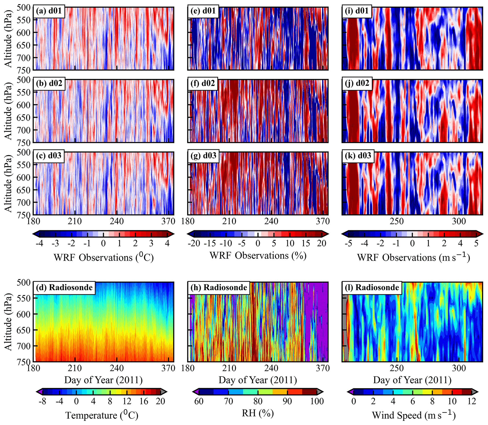
Figure 4Difference between model (d01: first row, d02: second row, d03: third row) and radiosonde observations for temperature (a, b, c), relative humidity (e, f, g), and wind speed (i, j, k) profiles up to 500 hPa. The fourth row provides the vertical profiles of radiosonde measurements. The x axis in panels (a–h) shows the day of the year in 2011 from 1 July (182nd day) to 30 September (273rd day). Wind speed (m s−1) profiles in panels (i–l) are provided for September 2011.
Figure 5 shows the vertical profiles of the following statistical metrics for the three simulations (d01, d02, d03): mean bias (MB), root mean square error (RMSE), and correlation coefficient (r) for temperature, relative humidity, and wind speed. The magnitudes of the MB values throughout the troposphere are estimated to be within about 1 ∘C, 12 %, and 2.5 m s−1 for temperature, relative humidity, and wind speed, respectively. Additionally, RMSE values are about 1 ∘C, 15 %–30 %, and 2.5–5 m s−1 for temperature, relative humidity, and wind speed, respectively. As discussed earlier, correlations between model results and observations are found to be stronger in the middle and upper troposphere than in the lower troposphere. For temperature, the r values are higher than 0.75 between 600 and 200 hPa, whereas they decrease to 0.4 at lower altitudes, i.e., near 800 hPa. Correlations in the lower troposphere are notably weaker (r = ∼ 0.25) in the case of wind speed. The results suggest that the model captures the day-to-day variabilities well in the meteorological parameters in the middle and upper troposphere and to a minor extent in the lower troposphere. Relatively weaker correlations in the lower troposphere are suggested to be associated with more pronounced effects of the uncertainties caused by the underlying complex mountain terrain and resulting unresolved local effects. Wind fields near the surface are strongly impacted by interactions between the terrain and boundary layer in addition to orographic drag in a modeling study over the Tibetan Plateau (Zhou et al., 2018) and in measurements over the Himalaya (Solanki et al., 2019). An increase in bias with altitude was reported by Kumar et al. (2012) for dew point temperature. Besides the model physics, the higher uncertainties in radiosonde humidity observations might have also contributed to these differences. The effect of model resolution is not very significant for temperature and wind profiles above 800 hPa; nevertheless, the mean bias for RH is lower (∼ 5 %) in the 800–600 hPa altitude range and higher in the 450–300 hPa altitude range in the d02 and d03 simulations. This might be due to deep convection in the model at a higher resolution. Overall, the model captured the vertical structures of meteorological parameters; however, a better representation of complex terrain is insufficient to improve the model performance aloft. On top of the better representation of topography as considered here, it highlights the need for future studies evaluating various physics scheme. Nevertheless, model biases have been significantly reduced for surface-level meteorology with higher resolution, and the details are discussed in the subsequent section.

Figure 5The vertical profiles of the mean bias (MB), root mean square error (RMSE), and correlation coefficient (r) for temperature, relative humidity, and wind speed in the different domains d01 (blue), d02 (red), and d03 (green).
3.3 Comparison with ground-based observations
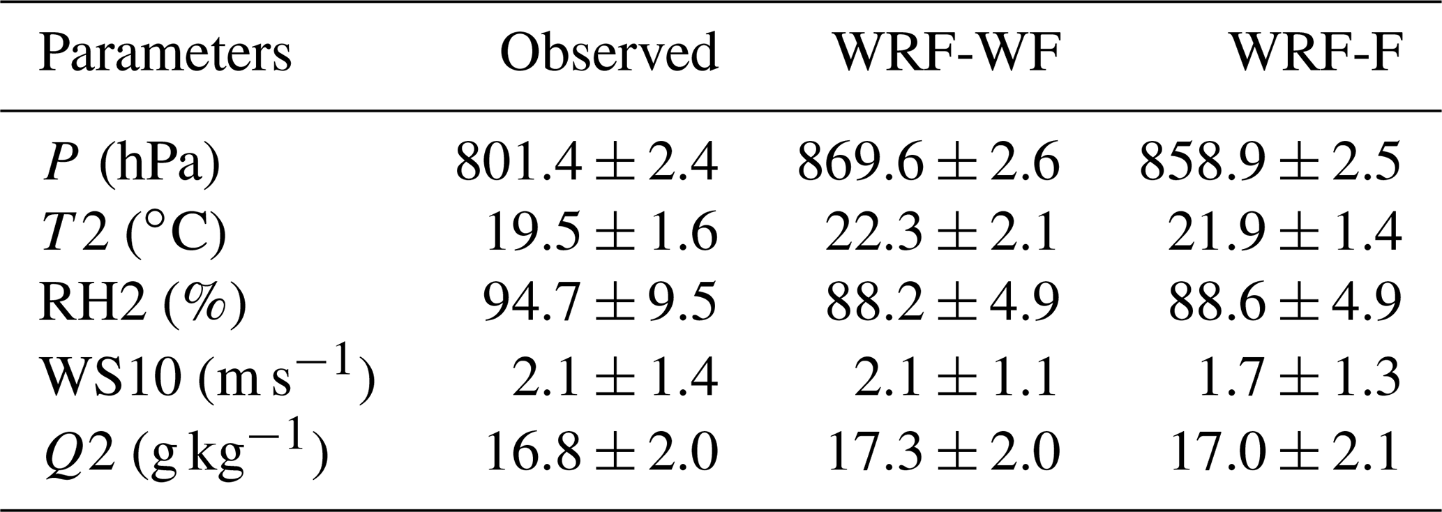
The model-simulated 2 m temperature (T2), 2 m relative humidity (RH2), and 10 m wind speed (WS10) for the observational site, Manora Peak, are compared with the ground-based measurements made during the GVAX campaign in Fig. 6 and summarized in Table 1. The diurnal variations in T2, RH2, and WS10 simulated by the WRF model are compared with observations, whereas the surface pressure does not show a significant diurnal variation (not shown here). Model simulation d01 shows a positive bias of 68 hPa in surface pressure, with a strong correlation (r = 0.97) with observations (mean = ∼ 801 hPa). A significant improvement is achieved (MB = 26 hPa) in d03 as a result of the finest-resolution simulation (Fig. 6 and Table 1). The WRF-model-simulated T2 shows a warm bias in all three domains. The simulated T2 for d01 varies from 16.2 to 28.7 ∘C, with a higher mean value of 22.3 ± 2.1 ∘C compared to the observed mean value of 19.5 ± 1.6 ∘C and a correlation of r = 0.75 between d01 and observations. This warm bias is seen to decrease from d01 (2.8 ∘C) to 0.2 ∘C with increasing model resolution in the d03 simulation (Table S1). The mean value of the RH2 in d01 is about 88.2 ± 9.7 %, which is 6.4 % lower than the observed value of 94.7 ± 9.5 % with a correlation of about 0.45 (Fig. 7b). MB and RMSE values of RH2 show a decrease with increasing model resolution (Table S1). As relative humidity also depends on temperature, the diurnal variation in 2 m specific humidity (Q2; g kg−1) has also been analyzed (Fig. S3). Q2 is observed in the range of 5.5–21.5 g kg−1 with a mean value of 16.8 ± 2.0 g kg−1. It is found that the agreement in Q2 is relatively better (MB = −0.7 g kg−1; r = 0.77 in d03) when the statistical metrics are compared with those for RH2 (Table S1). The wind speed plays a vital role in transport processes and controls the dynamics of the atmosphere at different temporal and spatial scales. The average 10 m wind speed (WS10) during the monsoon over the measurement station is about 2.1 ± 1.4 m s−1, which is quite comparable to that simulated in d01 (2.1 ± 1.1 m s−1), whereas it is overestimated in d02 by 0.9 m s−1 and in d03 by 0.5 m s−1 (Tables 1 and S1). In the case of the WS10, the correlation is 0.18 for d01 and d02, which improves to 0.24 in d03. The diurnal variation of WS10 (Fig. 6c) is not well captured, especially during noontime.
Table 1The mean (±standard deviation) along with the minimum and maximum values of the meteorological parameters surface pressure (P; hPa), 2 m temperature (T2; ∘C); 2 m relative humidity (RH2; %), and 10 m wind speed (WS10; m s−1) in the model simulations and observations for the full observation period. An additional evaluation is presented, accounting for the difference in model surface altitude and the actual altitude of measurements (referred to as “with altitude adjustment”).
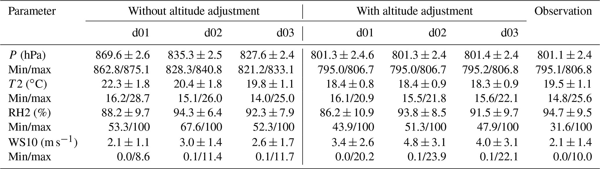
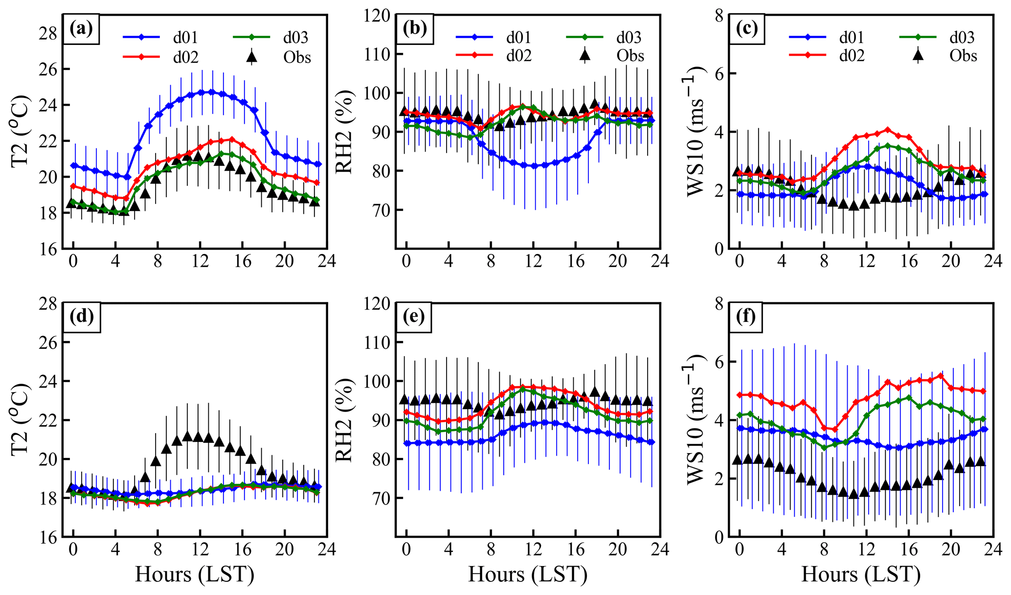
Figure 6Mean diurnal variations of (a) 2 m temperature (T2), (b) 2 m relative humidity (RH2), and (c) 10 m wind speed (WS10) from model simulations (d01, d02, and d03) and observations. Altitude-adjusted variations are also shown (d–f). The bars represent the standard deviation and are shown only for domain d01 and the observations in order to avoid overlap.
Due to the complex terrain and the grid size of the model, the simulated altitude of the observational site could differ from reality. In this study, the model underestimated station altitude by about 588, 480, and 270 m in d01, d02, and d03. We performed an additional evaluation to explore and achieve possible improvement by linearly interpolating the vertical profile of meteorological parameters to the actual altitude of the station (Fig. 6d–f), as done in a few previous studies (e.g., Mues et al., 2018). The altitude adjustment was made as per the equation of linear interpolation given in the Supplement (Eq. 4). The analysis shows that the correlation coefficient values between the model and observations do not show any clear improvement in model output (e.g., for T2 the correlation coefficient is 0.35) on adjusting the altitude except for WS10. After adjusting the altitude, the temperature variability is suppressed by the model at diurnal (Fig. 6a, d) and day-to-day timescales; i.e., r drops from 0.67 to 0.36 in d03. The comparison of temperature among the three domains for additional model layers has also been analyzed (Fig. S4). The diurnal amplitudes are seen to be smaller at higher model layers. Additionally, the differences among different simulations (d01, d02, and d03) also decrease at higher layers. As expected, the altitude adjustment does reduce the bias in pressure. Nevertheless, reductions in mean biases are not achieved (Table S1); instead, the absolute values of biases increase from 0.2 to 1.2, 2.4 to 3.1, 0.5 to 1.9, and 0.7 to 1.6 in T2, RH2, WS10, and Q2 in simulation d03. Besides thermal and mechanical interactions of mountain surfaces with the atmosphere, local processes such as evaporation and transpiration affect the near-surface meteorological conditions. A reduction in wind speed during the daytime is associated with the competing effects of mountain–valley circulations due to heating of the slopes versus synoptic-scale flows (Solanki et al., 2019). To resolve such sub-grid-scale processes, we emphasize that very high-resolution simulations are needed, as conducted in this study, in order to simulate the meteorological variability in a satisfactory way. The analysis further highlights the need for accurate representation of the complex topographical features rather than altitude-adjusted estimations, which led to very limited improvements in this case. However, we will discuss the evaluation without altitude adjustment unless stated otherwise.
We evaluate the MB values (Tables 1 and S1) in model simulations considering the benchmarks suggested by Emery et al. (2001). In the d03 simulation, MB values for both T2 (0.2 ∘C) and Q2 (−0.7 g kg−1) are found to be well within the range of benchmark values: ±0.5 ∘C for T2 and ±1.0 g kg−1 for Q2. It is important to note that biases in T2 in the coarser simulations d01 (2.8 ∘C) and d02 (0.9 ∘C) are, however, higher compared to the benchmarks. MB values in T2 estimated for this representative Himalayan site are found to be slightly lower (+0.2 ∘C) (−1.2 ∘C with altitude adjustment) than those over the Tibetan Plateau (−2 to −5 ∘C) (Gao et al., 2015) and over mountainous regions in the Europe (Zhang et al., 2013). The warmer bias in our case is due to underestimation of the Himalayan altitude, whereas the model overestimated terrain height over the Tibetan Plateau region, giving contrasting results. Further, the RMSE in wind speed is lower (1.6–2.0 m s−1) than that over the Kathmandu valley (2.2 m s−1; Mues et al., 2018) and similar to the benchmark (2.0 m s−1). Mar et al. (2016) also reported a similar bias (2 m s−1) in the 10 m wind speed over Europe and an average correlation of ∼ 0.4–0.6 over the Alps. Nevertheless, simulating the diurnal variation of near-surface winds still remains challenging over complex terrain, but the bias was reduced after including effects of the turbulent orographic form drag (Zhou et al., 2017, 2019). Besides turbulent orographic form drag, it is suggested that wind speed is sensitive to boundary layer schemes (Yver et al., 2013; Zhou et al., 2019) and that more studies are needed to explore these aspects over the central Himalaya.
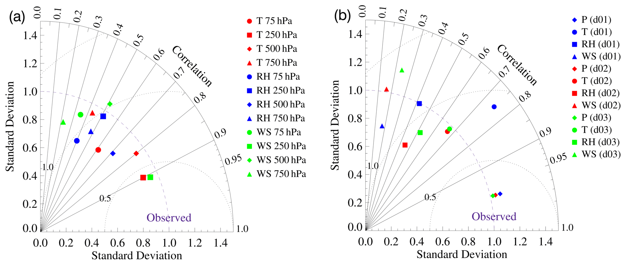
Figure 7Taylor diagram with the correlation coefficient, normalized standard deviation, and normalized root mean square difference (RMSD) error for (a) model performance at the different pressure levels shown in Fig. 3 for d01. (b) The model-simulated surface pressure, 2 m temperature, RH, and 10 m wind speed for different domains as shown in Fig. 6a–c.
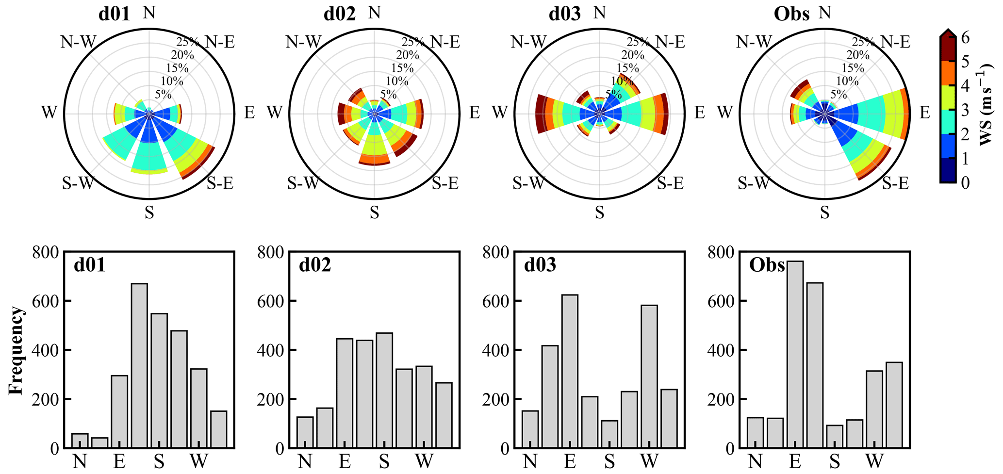
Figure 8Comparison of the wind speed and direction represented by the wind rose (top panel) and the frequency distribution of the wind direction (bottom panel) for model simulations over the three domains (d01, d02, d03) and observations (obs) during June–September 2011. Different colors and radii of wind roses show the wind speed and frequency of occurrences, respectively.
The wind direction is strongly influenced by the surrounding topography over mountainous regions, and the evaluation of the wind direction at horizontal resolution is depicted in Fig. 8. The winds varying between meteorological directions 337.5 and 22.5∘ are considered to be northerly and are represented by N in the frequency distribution and so on for other directional flow, referring to the clockwise meteorological convention. The wind flow dominance over the observational site is easterly (30 %) and southeasterly (26 %), while 26 % of wind occurrences are from the west and northwest. The percentage of southerly (21 %) and southwesterly winds (SW, 19 %) is relatively higher in d01 compared to the observations (S: 4 % and SW: 5 %) and decreases to 4 % and 9 % in d03. The model is able to simulate the northerly and northeasterly winds in d01 and d02, while the model simulates a larger contribution of northeasterly and westerly winds in d03, which is not seen in the observations. The easterly component of the model-simulated wind shows better agreement with observations on increasing the model resolution. In addition, the model is able to simulate the westerly and northwesterly wind contribution in d02, whereas the westerly component is overpredicted by 10 % in d03. The observations show that winds blowing from the north, northeast, south, and southwest are very weak (<2 m s−1) and amount to about ∼ 15 % of the total occurrences. The diurnal variation of the wind direction is not investigated here; however, the impact of mountain topography on the near-surface flow under low wind conditions has been discussed elsewhere (Solanki et al., 2019). Overall, the simulated wind field in d03 is in relatively better agreement with observations than d01 and d02. This is further assessed in Sect. 3.5 using a finer-resolution simulation by implementing SRTM3s terrain data.
3.4 Effect of feedback
In the preceding section, the simulations were carried out without any feedback (WRF-WF) from the finer-resolution domain to its parent domain, and results have been discussed. This WRF-WF experiment was conducted in such a way that it could explicitly account for the grid resolution effects on the model performance. The simulated meteorology with this model setup (with feedback) depicted different model performance in the outermost coarse-resolution domain d01 compared to d02 and d03. The model performance depends upon the boundary and initial conditions. Another model simulation is carried out in this section using the same configuration but with two-way interactive nesting and feedback (WRF-F) from the nested domain to its parent domain. The simulated meteorological parameters in the higher nests are fed back to their parent domains, and the boundary conditions are replaced there. The model results over the CH region in the regional-scale simulation (d01) show better agreement with the observations because of the feedback from the high-resolution nested simulation. The comparison of the simulated meteorological parameters (T2, RH2, and WS10) for the outermost domain with surface observations is presented in Fig. 9 for both WRF-WF and WRF-F simulations, thus showing the effect of feedback within the outermost domain.
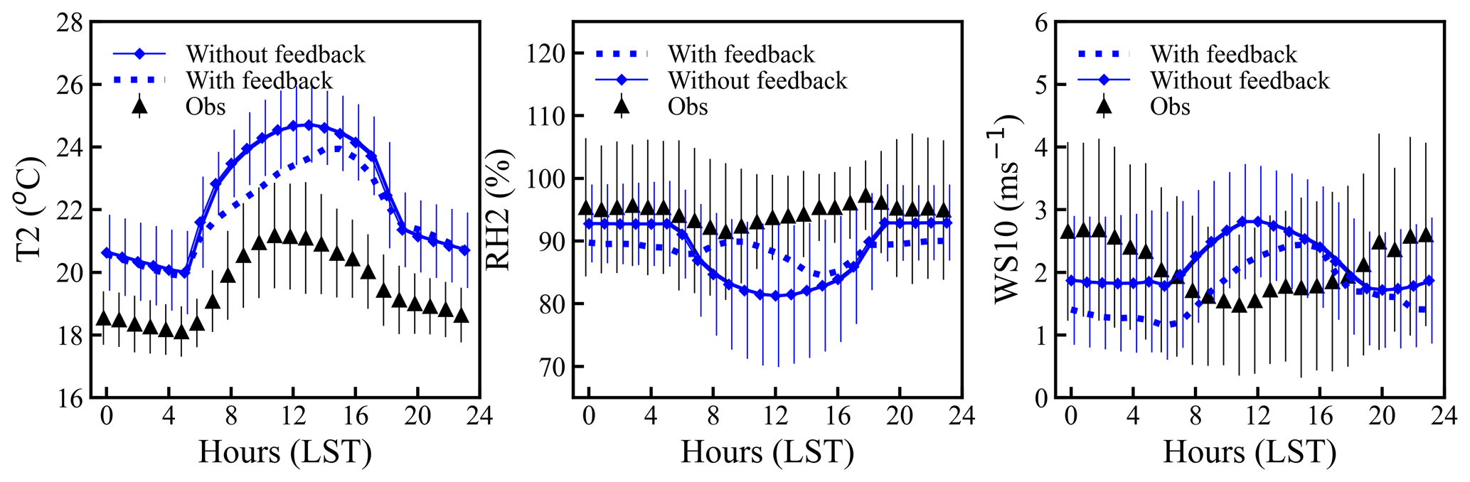
Figure 9Diurnal variation of the T2, RH2, and WS10 from d01 without feedback (WRF-WF) and with feedback (WRF-F). The bars represent the standard deviation and are shown only for domain d01 and observations in order to avoid overlap.
The comparison of mean values (Table 2) shows a decrease in model bias for T2, RH2, and Q2 by 0.5 ∘C, 0.3 %, and 0.2 g kg−1, respectively, due to feedback from finer-resolution simulations. Additionally, correlations are found to show improvements for RH2 and Q2 by 0.15 and 0.12, respectively, due to feedback; hence, the diurnal variation of relative humidity is closer to the observations (Fig. 9). Nevertheless, smaller changes were seen in correlations for WS10 (by 0.05) and T2 (by −0.02) (Fig. S5). Variations in wind speed and direction also show significant improvements, especially in the dominant flow direction, e.g., east, west, and northwest (Fig. S6).
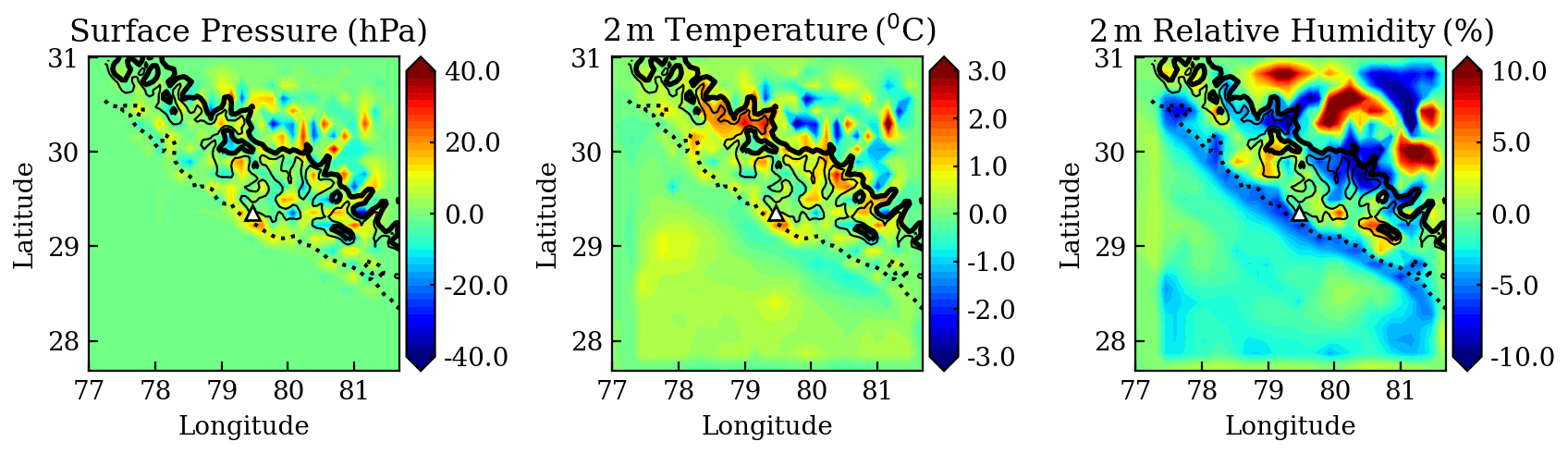
Figure 10The effect of the two-way nesting on d01 is shown. The difference between the simulations with feedback (WRF-F) and without feedback (WRF-WF) is shown for surface pressure, 2 m temperature, and 2 m relative humidity along with three elevation contours at 500 m (dashed), 1500 m (thin solid), and 2000 m (thick solid).
Table 2Comparison of the simulated meteorology for surface pressure (P), 2 m temperature (T2), 2 m relative humidity (RH2), 10 m wind speed (WS10), and 2 m specific humidity (Q2) to the observations in the outermost domain d01 for two model simulations: WRF-WF and WRF-F.
Effects of the feedback on surface pressure, 2 m temperature, and relative humidity in the domain d01 are shown by Fig. 10. Feedback effects are seen to be more pronounced over the mountainous region than over the flat terrain of the IGP. The feedback from the nested domain to the parent domain mostly modifies the meteorology over the mountainous region, as shown by the topography contours in Fig. 10. The analyses of biases and correlations suggest an improvement in the model-simulated pressure, temperature, and humidity through feedback from well-resolved nests. This further underpins the fact that better representations of the Himalaya over local scales can be adopted to simulate meteorology at the regional scale with lower biases over complex terrain in the given domain. Nevertheless, further modeling studies along with more observations are needed to improve the model performance. We extended the efforts to improve the wind speed and direction simulated over the complex topography by implementing a high-resolution (3 s) topographical input in the model to evaluate finer-resolution features over the Himalaya in the following section.
3.5 Inclusion of high-resolution (3 s) SRTM topography
Simulations described in previous sections were performed using the 30 s (∼ 1 km) topographic data from the GMTED2010 (Danielson and Gesch, 2011), which is comparable to the highest resolution of the WRF simulation (d03). In order to evaluate the influences of topographical features on the wind flow at finer scales, the topography input available at very high resolution (3 s or ∼ 90 m) from the Shuttle Radar Topography Mission (SRTM3s) (Farr et al., 2007) has been utilized. However, retaining the same model configuration as earlier, an additional innermost nest d04 having a resolution of ∼ 333 m, as depicted in Fig. 1 (bottom right panel), is included. Simulations with SRTM data at 1 km resolution did not differ significantly from the simulation with a similar resolution using GMTED2010 (GMTED hereafter). For this experiment, model simulation is performed only for September 2011. This simulation is carried out without feedback and compared with the observation to check the effect of implementing high-resolution topography.
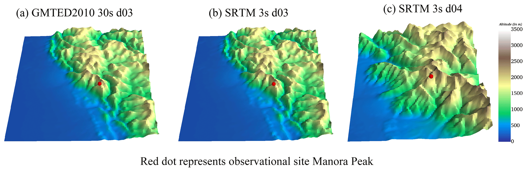
Figure 11The topography from GMTED at 30 s in domain d03 (a), SRTM at 3 s in domain d03 (b), and SRTM at 3 s in domain d04 (c). The model elevations of the observational site in d03 and d04 are 1670 and 1876 m, respectively.
The comparison of the topographic height between GMTED and SRTM3s in Fig. S7 shows that the differences are larger over the mountainous region, which vary from −100 to +100 m. The differences are suppressed within d02 and d03 as the topography input is changed from the GMTED to SRTM3s datasets. The topography in d04 (Fig. 11c) becomes resolved better and is marked by sharp variations of mountain ridges and valleys using the SRTM3s compared to d03, which are smoothed out with GMTED (Fig. 11a) or with SRTM3s interpolated to 1 km (Fig. 11b). After including the SRTM3s topography, the MB value for wind speed in d03 is found to show a slight reduction (∼ 0.04 m s−1). Also, the flow from various directions exhibited an improvement of 1 %–2 % with the use of SRTM3s (Table S2).
In d04, surface pressure is seen to be simulated more realistically (809 hPa), and the dry bias in 2 m relative humidity is improved by ∼ 2 % (Fig. S8 and Table S2). Simulations of diurnal wind variations remain challenging (not shown here) even at the finest resolutions considered (d04) utilizing the updated topographic data (SRTM3s). Further, to understand the effect of SRTM3s data on d04, the wind direction is compared with that in d03 and observations. The variations in winds are analyzed and shown by a wind rose (Fig. 12a–d) and frequency distribution (Fig. 12e–h). The fraction of the northeasterly component in d04 with SRTM3s (5 %) is found to be comparable with observations (6 %), which was overestimated by 19 % (17 %) in d03 with GMTED (SRTM3s). The frequency of the southerlies improves with the increasing resolution of topography and better matches the observations. The observations show the prevalence of northwesterly (19 %), easterly (24 %), westerly (18 %), and southeasterly (20 %) winds, and these are also seen to be the dominant directions in the simulation d04, with the exception of southeasterly winds.
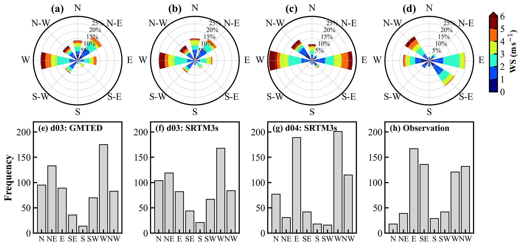
Figure 12Wind roses for (a) d03 using GMTED, (b–c) d03 and d04 using SRTM3s topography data, and (d) surface observations. The corresponding frequency distributions of the wind directions are shown in (e–f). The comparison of the wind speed and direction is shown for the month of September in 2011.
Simulation of the wind directions improved from d03 to d04 by using the SRTM3s topography, except certain wind directions such as southeasterly. An improvement is noticed in simulated surface pressure, 2 m relative humidity, and 10 m wind speed using the SRTM3s topography. Topographical data at different resolutions are found to show RH differences in the range of −1 % to 1 % in d02 and −3 % to 3 % in d03 (Fig. S9). Differences in simulated RH could be associated with the multi-scale orographic variations, which are found to be the key factors in meteorological simulation over complex terrain (e.g., Wang et al., 2020). The effects of the SRTM3s topographic static data have been studied previously over other regions of the world (e.g., Teixeira et al., 2014; De Meij and Vinuesa, 2014). However, the lower daytime wind speed and the transition phases during morning and evening hours still remain a challenge, even after using the high-resolution (333 m × 333 m) nest. Such discrepancies between the model and observations over the Himalayan region are suggested to be associated with still unresolved terrain features, in addition to the influences of input meteorological fields and the model physics on simulated atmospheric flows (e.g., Xue et al., 2014; Vincent and Hahmann, 2015).
This study using the WRF model mainly elucidated upon the various diagnostics it calculates for its multiple domains, the comparison of model results to an intensive field campaign, and downscaling to a sub-kilometer resolution with 3 s resolution SRTM topography data that resolves individual peaks and valleys over the CH region. The effects of spatial resolution on model-simulated meteorology have been examined by combining the WRF model with ground-based and in situ observations, as well as reanalysis datasets. Owing to the highly complex topography of the central Himalaya, model results show strong sensitivity towards the model resolution and adequate representation of terrain features. Model-simulated meteorological profiles do not show much dependency on the resolution, except in the lower atmosphere, which is directly influenced by terrain-induced effects and surface characteristics, emphasizing the need to evaluate various physics schemes over this region. The biases in 2 m temperature, relative humidity, and surface pressure show a decrease on increasing the model resolution, indicating a better-resolved representation of topographical features. Diurnal variations in meteorological parameters also show better agreement on increasing the grid resolution. Although the surface pressure does not show a pronounced diurnal variation, the biases in simulated surface pressure are significantly reduced over fine-resolution simulations. Interpolation of coarser simulations (d01, d02) to the station altitude reduces the bias in surface pressure and temperature, but it suppresses the diurnal variability. The results highlight the significance of accurately representing terrains at finer resolutions (d03). The model is generally not able to reproduce the frequency distribution of the wind direction, except in some of the major components in all the simulations with varying resolutions. The directionality of the simulated winds shows improvements over finer grid resolutions; however, reproducing the diurnal variability still remains a challenge. Biases are stronger typically during daytime and also during transitions of low to high wind conditions and vice versa. This is attributed to the uncertainties in representing the interaction of slope winds with the synoptic mean flow and local circulations, despite an improved representation of terrain features. A sensitivity experiment with domain feedback turned on shows that the feedback process can improve the representation of the CH in simulations covering a larger region of the northern Indian subcontinent. It is suggested that further improvements in the model performance are limited due to the lack of high-resolution topographical biases through input meteorological fields and model physics. Nevertheless, the implementation of a very high-resolution (3 s) topographical input using the SRTM data shows the potential to reduce the biases related to topographical features to some extent.
Observational data from the GVAX campaign are freely available (https://adc.arm.gov/discovery/#v/results/s/fsite::pgh.M, Kotamarthi, 2013). WRF is an open-source and publicly available model, which can be downloaded at http://www2.mmm.ucar.edu/wrf/users/download/get_source.html (Skamarock et al., 2008). A zip file containing (a) namelists for both the preprocessor (WPS) and the WRF (b) 3 s resolution topography input prepared for the pre-processor, along with a README file describing the necessary details to perform the simulations, has been archived at https://doi.org/10.5281/zenodo.3978569 (Singh and Ojha, 2020).
The supplement related to this article is available online at: https://doi.org/10.5194/gmd-14-1427-2021-supplement.
NS and AP designed and supervised the study. JS performed the simulations, assisted by NO and AS. JS, NO, and AS analyzed the model results, and NKK, KR, and SSG contributed to the interpretations. VRK significantly contributed to conceiving and realizing the GVAX campaign. JS and NS wrote the first draft, and all the authors contributed to the paper.
The authors declare that they have no conflict of interest.
We are thankful to the director of ARIES, Nainital. We acknowledge NCAR for the WRF-ARW model, ECMWF for the ERA-Interim reanalysis datasets, and the ARM Climate Research Facility of the U.S. Department of Energy (DOE) for the observations made during the GVAX campaign. Computing resources from the Max Planck Computing and Data Facility (MPCDF) are profoundly acknowledged. Narendra Ojha acknowledges the computing resources Vikram-100 HPC at the Physical Research Laboratory (PRL) and valuable support from Duggirala Pallamraju and Anil Bhardwaj. Constructive comments and suggestions from the anonymous reviewers and the handling editor are gratefully acknowledged.
Jaydeep Singh is the senior research fellow for the ABLN&C:NOBLE project under ISRO-GBP.
The article processing charges for this open-access
publication were covered by the Max Planck Society.
This paper was edited by Juan Antonio Añel and reviewed by three anonymous referees.
Angevine, W. M., Bazile, E., Legain, D., and Pino, D.: Land surface spinup for episodic modeling, Atmos. Chem. Phys., 14, 8165–8172, https://doi.org/10.5194/acp-14-8165-2014, 2014.
Bhutiyani, M. R., Kale, V. S., and Pawar, N. J.: Long-term trends in maximum, minimum and mean annual air temperatures across the Northwestern Himalaya during the twentieth century, Climatic Change, 85, 59–177, https://doi.org/10.1007/s10584-006-9196-1, 2007.
Bonasoni, P., Cristofanelli, P., Marinoni, A., Vuillermoz, E., and Adhikary, B.: Atmospheric pollution in the Hindu Kush-Himalaya region: Evidence and implications for the regional climate, Mt. Res. Dev., 32, 468–479, 2012.
Boyle, J. and Klein, S. A.: Impact of horizontal resolution on climate model forecasts of tropical precipitation and diabatic heating for the TWP-ICE period, J. Geophys. Res.-Atmos., 115, D23113, https://doi.org/10.1029/2010JD014262, 2010.
Cannon, F., Carvalho, L. M. V., Jones, C., Norris, J., Bookhagen, B., and Kiladis, G. N.: Effects of topographic smoothing on the simulation of winter precipitation in High Mountain Asia, J. Geophys. Res.-Atmos., 122, 1456–1474, https://doi.org/10.1002/2016JD026038, 2017.
Caya, D. and Laprise, R.: A semi-implicit semi-Lagrangian regional climate model: The Canadian RCM, Mon. Weather Rev., 127, 341–362, https://doi.org/10.1175/1520-0493(1999)127<0341:ASISLR>2.0.CO;2, 1999.
Chen, F. and Dudhia, J.: Coupling an advanced land surface – hydrology model with the Penn State – NCAR MM5 modeling system. Part I: Model implementation and sensitivity, Mon. Weather Rev., 129, 569–585, https://doi.org/10.1175/1520-0493(2001)129<0569:CAALSH>2.0.CO;2, 2001.
Cheng, W. Y. Y. and Steenburgh, W. J.: Evaluation of surface sensible weather forecasts by the WRF and the Eta Models over the western United States, Weather Forecast., 20, 812–821, https://doi.org/10.1175/WAF885.1, 2005.
Chou, M. D. and Suarez, M. J.: An efficient thermal infrared radiation parameterization for use in general circulation models, NASA Technical Memorandum No. 104606 Vol. 3, NASA, Washington D. C., USA, 85 pp., 1994.
Christensen, J. H., Christensen, O. B., Lopez, P., van Meijgaard, E., and Botzet, M.: The HIRHAM4 regional atmospheric climate model, DMI Scientific report 4, DMI, Copenhagen, Denmark, 51 pp., 1996.
Danielson, J. J. and Gesch, D. B.: Global multi-resolution terrain elevation data 2010 (GMTED2010) (No. 2011-1073), US Geological Survey, Reston, Virginia, USA, 26 pp., 2011.
Dee, D. P., Uppala, S. M., Simmons, A. J., Berrisford, P., Poli, P., Kobayashi, S., Andrae, U., Balmaseda, M. A., Balsamo, G., Bauer, D. P., and Bechtold, P.: The ERA-Interim reanalysis: Configuration and performance of the data assimilation system, Q. J. Roy. Meteor. Soc., 137, 553–597, https://doi.org/10.1002/qj.828, 2011.
Deep, A., Pandey, C. P., Nandan, H., Purohit, K. D., Singh, N., Singh, J., Srivastava, A. K., and Ojha, N.: Evaluation of ambient air quality in Dehradun city during 2011–2014, J. Earth Syst. Sci., 128, 96, https://doi.org/10.1007/s12040-019-1092-y, 2019.
De Meij, A. and Vinuesa, J. F.: Impact of SRTM and Corine Land Cover data on meteorological parameters using WRF, Atmos. Res., 143, 351–370, https://doi.org/10.1016/j.atmosres.2014.03.004, 2014.
Dimri, A. P., Chevuturi, A., Niyogi, D., Thayyen, R. J., Ray, K., Tripathi, S. N., Pandey, A. K., and Mohanty, U. C.: Cloudbursts in Indian Himalayas: a review, Earth-Sci. Rev., 168, 1–23, https://doi.org/10.1016/j.earscirev.2017.03.006, 2017.
Dumka, U. C., Kaskaoutis, D. G., Sagar, R., Chen, J., Singh, N., and Tiwari, S.: First results from light scattering enhancement factor over central Indian Himalayas during GVAX campaign, Sci. Total Environ., 605/606, 124–138, https://doi.org/10.1016/j.scitotenv.2017.06.138, 2017.
Ek, M. B., Mitchell, K. E., Lin, Y., Rogers, E., Grunmann, P., Koren, V., Gayno, G., and Tarpley, J. D.: Implementation of Noah land surface model advances in the National Centers for Environmental Prediction operational mesoscale Eta model, J. Geophys. Res.-Atmos., 108, D228851, https://doi.org/10.1029/2002JD003296, 2003.
Emery, C., Tai, E., and Yarwood, G.: Enhanced meteorological modeling and performance evaluation for two Texas ozone episodes, Technical Report, Texas Natural Resource Conservation Commission, ENVIRON International Corporation, Work Assignment No. 31984-11, ENVIRON International Corporation, Novato, CA, 235 pp., 2001.
Farr, T. G., Rosen, P. A., Caro, E., Crippen, R., Duren, R., Hensley, S., Kobrick, M., Paller, M., Rodriguez, E., Roth, L., and Seal, D.: The shuttle radar topography mission, Rev. Geophys., 45, RG2004, https://doi.org/10.1029/2005RG000183, 2007.
Foley, A. M.: Uncertainty in regional climate modelling: A review, Prog. Phys. Geog., 34, 647–670, https://doi.org/10.1177/0309133310375654, 2010.
Gao, Y., Xu, J., and Chen, D.: Evaluation of WRF mesoscale climate simulations over the Tibetan Plateau during 1979–2011, J. Climate, 28, 2823–2841, https://doi.org/10.1175/JCLI-D-14-00300.1, 2015.
Hanna, S. R. and Yang, R.: Evaluations of Mesoscale Models' Simulations of Near-Surface Winds, Temperature Gradients, and Mixing Depths, J. Appl. Meteorol., 40, 1095–1104, https://doi.org/10.1175/1520-0450(2001)040<1095:EOMMSO>2.0.CO;2, 2001.
Hong, S. Y., Noh, Y., and Dudhia, J.: A new vertical diffusion package with an explicit treatment of entrainment processes, Mon. Weather Rev., 134, 2318–2341, https://doi.org/10.1175/MWR3199.1, 2006.
Jerez, S., López-Romero, J. M., Turco, M., Lorente-Plazas, R., Gómez-Navarro, J. J., Jiménez-Guerrero, P., and Montávez, J. P.: On the Spin-Up Period in WRF Simulations Over Europe: Trade-Offs Between Length and Seasonality, J. Adv. Model. Earth Syst., 12, e2019MS001945, https://doi.org/10.1029/2019MS001945, 2020.
Kain, J. S.: The Kain-Fritsch convective parameterization: an update, J. Appl. Meteorol., 43, 170–181, https://doi.org/10.1175/1520-0450(2004)043<0170:TKCPAU>2.0.CO;2 ,2004.
Kotamarthi, V. R.: Ganges Valley Aerosol Experiment (GVAX) Final Campaign Report DOE/SC-ARM-14-011, available at: https://adc.arm.gov/discovery/#v/results/s/fsite::pgh.M (last access: January 2021), 2013.
Kumar, A., Singh, N., Anshumali, and Solanki, R.: Evaluation and utilization of MODIS and CALIPSO aerosol retrievals over a complex terrain in Himalaya, Remote Sens. Environ., 206, 139–155, https://doi.org/10.1016/j.rse.2017.12.019, 2018.
Kumar, R., Naja, M., Pfister, G. G., Barth, M. C., and Brasseur, G. P.: Simulations over South Asia using the Weather Research and Forecasting model with Chemistry (WRF-Chem): set-up and meteorological evaluation, Geosci. Model Dev., 5, 321–343, https://doi.org/10.5194/gmd-5-321-2012, 2012.
Laprise, R.: Regional climate modelling, J. Comput. Phys., 227, 3641–3666, https://doi.org/10.1016/j.jcp.2006.10.024, 2008.
Lawrence, M. G. and Lelieveld, J.: Atmospheric pollutant outflow from southern Asia: a review, Atmos. Chem. Phys., 10, 11017–11096, https://doi.org/10.5194/acp-10-11017-2010, 2010.
Lee, T. J., Pielke, R. A., Kessler, R. C., and Weaver, J.: Influence of Cold Pools Downstream of Mountain Barriers on Downslope Winds and Flushing, Mon. Weather Rev., 117, 2041–2058, https://doi.org/10.1175/1520-0493(1989)117<2041:IOCPDO>2.0.CO;2, 1989.
Lelieveld, J., Bourtsoukidis, E., Brühl, C., Fischer, H., Fuchs, H., Harder, H., Hofzumahaus, A., Holland, F., Marno, D., Neumaier, M., and Pozzer, A.: The South Asian monsoon – pollution pump and purifier, Science, 361, 270–273, https://doi.org/10.1126/science.aar2501, 2018.
Mar, K. A., Ojha, N., Pozzer, A., and Butler, T. M.: Ozone air quality simulations with WRF-Chem (v3.5.1) over Europe: model evaluation and chemical mechanism comparison, Geosci. Model Dev., 9, 3699–3728, https://doi.org/10.5194/gmd-9-3699-2016, 2016.
Meher, J. K., Das, L., Akhter, J., Benestad, R. E., and Mezghani, A.: Performance of CMIP3 and CMIP5 GCMs to simulate observed rainfall characteristics over the Western Himalayan region, J. Climate, 30, 7777–7799, https://doi.org/10.1175/JCLI-D-16-0774.1, 2017.
Mlawer, E. J., Taubman, S. J., Brown, P. D., Iacono, M. J., and Clough, S. A.: Radiative transfer for inhomogeneous atmospheres: RRTM, a validated correlated-k model for the longwave, J. Geophys. Res.-Atmos., 102, 16663–16682, https://doi.org/10.1029/97JD00237, 1997.
Mues, A., Lauer, A., Lupascu, A., Rupakheti, M., Kuik, F., and Lawrence, M. G.: WRF and WRF-Chem v3.5.1 simulations of meteorology and black carbon concentrations in the Kathmandu Valley, Geosci. Model Dev., 11, 2067–2091, https://doi.org/10.5194/gmd-11-2067-2018, 2018.
Naja, M., Bhardwaj, P., Singh, N., Kumar, P., Kumar, R., Ojha, N., Sagar, R., Satheesh, S. K., Krishna Moorthy, K., and Kotamarthi, V. R.: High-frequency vertical profiling of meteorological parameters using AMF1 facility during RAWEX–GVAX at ARIES, Nainital, Curr. Sci., 111, 132–140, 2016.
Nandargi, S. and Dhar, O. N.: Extreme rainstorm events over the northwest Himalayas during 1875–2010, J. Hydrometeorol., 13, 1383–1388, https://doi.org/10.1175/JHM-D-12-08.1, 2012.
Norris, J., Carvalho, L. M. V., Jones, C., and Cannon, F.: Warming and drying over the central Himalaya caused by an amplification of local mountain circulation, NPJ Clim. Atmos. Sci., 3, 1, https://doi.org/10.1038/s41612-019-0105-5, 2020.
Ojha, N., Naja, M., Singh, K. P., Sarangi, T., Kumar, R., Lal, S., Lawrence, M. G., Butler, T. M., and Chandola, H. C.: Variabilities in ozone at a semi-urban site in the Indo-Gangetic Plain region: Association with the meteorology and regional processes, J. Geophys. Res.-Atmos., 117, D20301, https://doi.org/10.1029/2012JD017716, 2012.
Ojha, N., Pozzer, A., Rauthe-Schöch, A., Baker, A. K., Yoon, J., Brenninkmeijer, C. A. M., and Lelieveld, J.: Ozone and carbon monoxide over India during the summer monsoon: regional emissions and transport, Atmos. Chem. Phys., 16, 3013–3032, https://doi.org/10.5194/acp-16-3013-2016, 2016.
Ojha, N., Girach, I., Sharma, K., Nair, P., Singh, J., Sharma, N., Singh, N., Flemming, J., Inness, A., and Subrahmanyam, K. V.: Surface ozone in the Doon Valley of the Himalayan foothills during spring, Environ. Sci. Poll. Res., 26, 19155–19170, https://doi.org/10.1007/s11356-019-05085-2, 2019.
Pant, G. B., Pradeep Kumar, P., Revadekar, J. V., and Narendra Singh: The Himalaya, in: Climate Change in the Himalayas, Springer Nature, Cham, Switzerland, 39-62 pp., https://doi.org/10.1007/978-3-319-61654-4, 2018.
Pervez, M. S. and Henebry, G. M.: Projections of the Ganges-Brahmaputra precipitation – Downscaled from GCM predictors, J. Hydrol., 517, 120–134, https://doi.org/10.1016/j.jhydrol.2014.05.016, 2014.
Potter, E. R., Orr, A., Willis, I. C., Bannister, D., and Salerno, F.: Dynamical Drivers of the Local Wind Regime in a Himalayan Valley, J. Geophys. Res.-Atmos., 123, 13186–13202, https://doi.org/10.1029/2018JD029427, 2018.
Rupakheti, D., Adhikary, B., Praveen, P. S., Rupakheti, M., Kang, S., Mahata, K. S., Naja, M., Zhang, Q., Panday, A. K., and Lawrence, M. G.: Pre-monsoon air quality over Lumbini, a world heritage site along the Himalayan foothills, Atmos. Chem. Phys., 17, 11041–11063, https://doi.org/10.5194/acp-17-11041-2017, 2017.
Sarangi, T., Naja, M., Ojha, N., Kumar, R., Lal, S., Venkataramani, S., Kumar, A., Sagar, R., and Chandola, H. C.: First simultaneous measurements of ozone, CO, and NOy at a high-altitude regional representative site in the central Himalayas, J. Geophys. Res.-Atmos., 119, 1592–1611, https://doi.org/10.1002/2013JD020631, 2014.
Seck, A., Welty, C., and Maxwell, R. M.: Spin-up behavior and effects of initial conditions for an integrated hydrologic model, Water Resour. Res., 51, 2188–2210, https://doi.org/10.1002/2014WR016371, 2015.
Sharma, A., Ojha, N., Pozzer, A., Mar, K. A., Beig, G., Lelieveld, J., and Gunthe, S. S.: WRF-Chem simulated surface ozone over south Asia during the pre-monsoon: effects of emission inventories and chemical mechanisms, Atmos. Chem. Phys., 17, 14393–14413, https://doi.org/10.5194/acp-17-14393-2017, 2017.
Sharma, S. S. and Ganju, A.: Complexities of avalanche forecasting in Western Himalaya – an overview, Cold Reg. Sci. Technol., 31, 95–102, https://doi.org/10.1016/S0165-232X(99)00034-8, 2000.
Singh, J. and Ojha, N.: Singh_GMD_WRF-ARW v3.8.1, Zenodo, https://doi.org/10.5281/zenodo.3978569, 2020.
Singh, N., Solanki, R., Ojha, N., Janssen, R. H. H., Pozzer, A., and Dhaka, S. K.: Boundary layer evolution over the central Himalayas from radio wind profiler and model simulations, Atmos. Chem. Phys., 16, 10559–10572, https://doi.org/10.5194/acp-16-10559-2016, 2016.
Skamarock, W. C., Klemp, J. B., Dudhia, J., Gill, D. O., Barker, D. M., Wang, W., and Powers, J. G.: A Description of the Advanced Research WRF Version 3, NCAR Technical Note NCAR/TN-475+STR, Boulder, Colorado, USA, 113 pp., https://doi.org/10.5065/D68S4MVH, 2008 (data available at: http://www2.mmm.ucar.edu/wrf/users/download/get_source.html, last access: January 2021).
Solanki, R., Singh, N., Kumar, N. K., Rajeev, K., and Dhaka, S. K.: Time variability of surface-layer characteristics over a mountain ridge in the central Himalayas during the spring season, Bound.-Lay. Meteorol., 158, 453–471, https://doi.org/10.1007/s10546-015-0098-5, 2016.
Solanki, R., Singh, N., Kiran Kumar, N. V. P., Rajeev, K., Imasu, R., and Dhaka, S. K.: Impact of Mountainous Topography on Surface-Layer Parameters During Weak Mean-Flow Conditions, Bound.-Lay. Meteorol., 172, 133–148, https://doi.org/10.1007/s10546-019-00438-3, 2019.
Srivastava, A. K., Soni, V. K., Singh, S., Kanawade, V. P., Singh, N., Tiwari, S., and Attri, S. D.: An early South Asian dust storm during March 2012 and its impacts on Indian Himalayan foothills: A case study, Sci. Total Environ., 493, 526–534, https://doi.org/10.1016/j.scitotenv.2014.06.024, 2014.
Sun, X. B., Ren, G. Y., Shrestha, A. B., Ren, Y. Y., You, Q. L., Zhan, Y. J., Xu, Y., and Rajbhandari, R.: Changes in extreme temperature events over the Hindu Kush Himalaya during 1961–2015, Adv. Clim. Change Res., 8, 157–165, https://doi.org/10.1016/j.accre.2017.07.001, 2017.
Taylor, K. E.: Summarizing multiple aspects of model performance in a single diagram, J. Geophys. Res.-Atmos., 106, 7183–7192, https://doi.org/10.1029/2000JD900719, 2001.
Teixeira, J. C., Carvalho, A. C., Carvalho, M. J., Luna, T., and Rocha, A.: Sensitivity of the WRF model to the lower boundary in an extreme precipitation event – Madeira island case study, Nat. Hazards Earth Syst. Sci., 14, 2009–2025, https://doi.org/10.5194/nhess-14-2009-2014, 2014.
Tewari, M., Chen, F., Wang, W., Dudhia, J., LeMone, M. A., Mitchell, K., Ek, M., Gayno, G., Wegiel, J., and Cuenca, R. H.: Implementation and verification of the unified NOAH land surface model in the WRF model, in: Proceedings of the 20th conference on weather analysis and forecasting/16th conference on numerical weather prediction, Seatle, Washington, USA, 12–16 January, 2004, Article No. 17.5, 6 pp., 2004.
Thompson, G., Rasmussen, R. M., and Manning, K.: Explicit forecasts of winter precipitation using an improved bulk microphysics scheme. Part I: Description and sensitivity analysis, Mon. Weather Rev., 132, 519–542, https://doi.org/10.1175/1520-0493(2004)132<0519:EFOWPU>2.0.CO;2, 2004.
Tiwari, P. R., Kar, S. C., Mohanty, U. C., Dey, S., Sinha, P., and Shekhar, M. S.: Sensitivity of the Himalayan orography representation in simulation of winter precipitation using Regional Climate Model (RegCM) nested in a GCM, Clim. Dynam., 49, 4157–4170, https://doi.org/10.1007/s00382-017-3567-3, 2017.
Tselioudis, G., Douvis, C., and Zerefos, C.: Does dynamical downscaling introduce novel information in climate model simulations of precipitation change over a complex topography region?, Int. J. Climatol., 32, 1572–1578, https://doi.org/10.1002/joc.2360, 2012.
Vincent, C. L. and Hahmann, A. N.: The impact of grid and spectral nudging on the variance of the near-surface wind speed, J. Appl. Meteorol. Climatol., 54, 1021–1038, https://doi.org/10.1175/JAMC-D-14-0047.1, 2015.
Wang, Y., Leung, L. R., McGregor, J. L., Lee, D. K., Wang, W. C., Ding, Y., and Kimura, F.: Regional climate modeling: progress, challenges, and prospects, J. Meteorol. Soc. Jpn., 82, 1599–1628, https://doi.org/10.2151/jmsj.82.1599, 2004.
Wang, Y., Yang, K., Zhou, X., Chen, D., Lu, H., Ouyang, L., Chen, Y., Lazhu, and Wang, B.: Synergy of orographic drag parameterization and high resolution greatly reduces biases of WRF-simulated precipitation in central Himalaya, Clim. Dynam., 54, 1729–1740, https://doi.org/10.1007/s00382-019-05080-w, 2020.
Weisman, M. L., Skamarock, W. C., and Klemp, J. B.: The resolution dependence of explicitly modeled convective systems, Mon. Weather Rev., 125, 527–548, https://doi.org/10.1175/1520-0493(1997)125<0527:TRDOEM>2.0.CO;2, 1997.
Wilby, R. L., Hay, L. E., and Leavesley, G. H.: A comparison of downscaled and raw GCM output: implications for climate change scenarios in the San Juan River basin, Colorado, J. Hydrol., 225, 67–91, https://doi.org/10.1016/S0022-1694(99)00136-5, 1999.
Xue, Y., Janjic, Z., Dudhia, J., Vasic, R., and De Sales, F.: A review on regional dynamical downscaling in intraseasonal to seasonal simulation/prediction and major factors that affect downscaling ability, Atmos. Res., 147/148, 68–85, https://doi.org/10.1016/j.atmosres.2014.05.001, 2014.
Yver, C. E., Graven, H. D., Lucas, D. D., Cameron-Smith, P. J., Keeling, R. F., and Weiss, R. F.: Evaluating transport in the WRF model along the California coast, Atmos. Chem. Phys., 13, 1837–1852, https://doi.org/10.5194/acp-13-1837-2013, 2013.
Zadra, A., Caya, D., Côté, J. E. A. N., Dugas, B., Jones, C., Laprise, R., Winger, K., and Caron, L. P.: The next Canadian regional climate model, Phys. Can., 64, 75–83, 2008.
Zhang, D. L. and Zheng, W. Z.: Diurnal cycles of surface winds and temperatures as simulated by five boundary layer parameterizations, J. Appl. Meteorol., 43, 157–169, https://doi.org/10.1175/1520-0450(2004)043<0157:DCOSWA>2.0.CO;2, 2004.
Zhang, Y., Sartelet, K., Wu, S.-Y., and Seigneur, C.: Application of WRF/Chem-MADRID and WRF/Polyphemus in Europe – Part 1: Model description, evaluation of meteorological predictions, and aerosol–meteorology interactions, Atmos. Chem. Phys., 13, 6807–6843, https://doi.org/10.5194/acp-13-6807-2013, 2013.
Zhou, X., Beljaars, A., Wang, Y., Huang, B., Lin, C., Chen, Y., and Wu, H.: Evaluation of WRF Simulations With Different Selections of Subgrid Orographic Drag Over the Tibetan Plateau, J. Geophys. Res.-Atmos., 122, 9759–9772, https://doi.org/10.1002/2017JD027212, 2017.
Zhou, X., Yang, K., and Wang, Y.: Implementation of a turbulent orographic form drag scheme in WRF and its application to the Tibetan Plateau, Clim. Dynam, 50, 2443–2455, https://doi.org/10.1007/s00382-017-3677-y, 2018.
Zhou, X., Yang, K., Beljaars, A., Li, H., Lin, C., Huang, B., and Wang, Y.: Dynamical impact of parameterized turbulent orographic form drag on the simulation of winter precipitation over the western Tibetan Plateau, Clim. Dynam, 53, 707–720, https://doi.org/10.1007/s00382-019-04628-0, 2019.