Applying a new integrated mass-flux adjustment filter in rapid update cycling of convective-scale data assimilation for the COSMO model (v5.07)

A new integrated mass-flux adjustment filter is introduced, which uses the analyzed integrated mass-flux divergence field to correct the analyzed wind field. The filter has been examined in twin experiments with rapid update cycling using an idealized setup for convective-scale radar data assimilation. It is found that the new filter slightly reduces the accuracy of background and analysis states; however, it preserves the main structure of cold pools and primary mesocyclone properties of supercells. More importantly, it considerably diminishes spurious mass-flux divergence and the high surface pressure tendency, and it thus results in more dynamically balanced analysis states. For the ensuing 3 h forecasts, the experiment that employs the filter becomes more skillful after 1 h. These preliminary results show that the filter is a promising tool to alleviate the imbalance problem caused by data assimilation, especially for convective-scale applications.

1 Introduction

The performance of convective-scale data assimilation has been considerably enhanced in the last decades, greatly due to the usage of Doppler radar observations. Assimilation of radar data has been adopted in the operational mode in more and more meteorological centers (Gustafsson et al., 2018). Although weather radars provide observations in minutes, the typical update frequency at most operational centers is around 1 h. Besides the high computational expense, another reason for this can be the unphysical imbalance arising from rapid update cycling. For instance, Lange and Craig (2014) and Bick et al. (2016) investigated the impact of different update frequencies (5, 15, 30 and 60 min) and found that a higher update frequency results in model states that are closer to radar observations but less physically consistent (indicated by greater surface pressure tendency), and its forecast skills decay faster. In practice, a number of techniques prove to be effective in diminishing the unphysical imbalance and noise produced by data assimilation. The digital filter initialization (DFI; Lynch and Huang, 1992) and the weak digital filter constraint (Gauthier and Thepaut, 2001) are widely used (e.g., at Meteo-France and the Met Office) to damp high-frequency inertia–gravity and acoustic waves. Hydrostatic balancing of analysis increments (Rhodin et al., 2013) is implemented in the Kilometre-scale ENsemble Data Assimilation (KENDA; Schraff et al., 2016) system for the model of COSMO (COnsortium for Small-scale MOdelling; Baldlauf et al., 2011) at the DWD to suppress the noise that is visible in the surface pressure tendency. These temporal filtering and spatial balancing methods are derived for synoptic-scale processes and work successfully for synoptic-scale data assimilation. Currently, they are also often applied in mesoscale and convective-scale data assimilation, but their transferability onto those scales is debatable because the balance constraints may break down at high resolutions (Vetra-Carvalho et al., 2012), and high-frequency waves or unbalanced flow may be associated with mesoscale fronts or convective events. Another popular approach is incremental analysis update (IAU; Bloom et al., 1996; Lei and Whitaker, 2016), which distributes the analysis increments over the assimilation window. IAU has been used for synoptic- and convective-scale data assimilation (He et al., 2020; Milan et al., 2020); however, its performance for very short assimilation windows (i.e., several minutes) has not been investigated. Moreover, Zeng et al. (2017) developed an ensemble Kalman filter (EnKF) that imposes enstrophy conservation by using a strong global constraint and tested it with a 2D shallow-water model that mimics the Northern Hemisphere. It is shown that enstrophy conservation reduces the noise and improves the forecast skills. For the convective scale, Ruckstuhl and Janjić (2018) tested an EnKF-based algorithm that conserves mass with the modified 1D shallow-water model (Würsch and Craig, 2014) and found that mass conservation is effective at suppressing spurious convection. But these methods with strong constraints are very costly in terms of computational time, and essential efforts are still required to make them suitable for numerical weather prediction (NWP) models.

The surface pressure tendency is commonly regarded as a metric for dynamical imbalance. Typically, the surface pressure tendency in the analysis is several times greater than that in the background (e.g., Lange and Craig, 2014; Bick et al., 2016; Lange et al., 2017). Hamrud et al. (2015) introduced the surface pressure tendency as a model diagnostic variable in a global model of the ECMWF (European Centre for Medium-Range Weather Forecasts), and the analyzed surface pressure tendency was used to accordingly adjust the analyzed horizontal wind field, which finally resulted in very small wind increments and more balanced model states. However, this approach is underdetermined because of using one variable (the surface pressure tendency) to correct two components of the horizontal wind. Therefore, some ad hoc assumption must be additionally made. In this work, a similar approach is developed, but the increment of the horizontal wind field from the analyzed integrated mass-flux divergence and vorticity is calculated analytically. We name this new method “the integrated mass-flux adjustment filter” and examine it in a rapid update cycling of convective-scale data assimilation using an idealized setup of the KENDA system for the COSMO model with the data assimilation scheme of the local ensemble transform Kalman filter (LETKF; Hunt et al., 2007).

The paper is organized as follows. Section 2 describes the integrated mass-flux adjustment filter in detail. Section 3 provides a short introduction to the idealized setup of the COSMO-KENDA system and the experimental design. Section 4 gives experimental results, and the last section is devoted to the conclusion and outlook.

2 The integrated mass-flux adjustment filter

When observations are assimilated to correct the model state, shocks can occur, which produces very large surface pressure tendency and fast waves. This can be especially remarkable for the LETKF since it is a local method and does not respect spatial derivatives.

The atmospheric surface pressure is dominated by the hydrostatic pressure:

$$\begin{array}{}\text{(1)}& p_{\mathrm{s}}^{\mathrm{h}}\approx \underset{\mathrm{0}}{\overset{Z_{\mathrm{0}}}{\int }}\mathit{\rho }\left(z\right)g\mathrm{d}z,\end{array}$$

where the superscript “h” is for “hydrostatic”, g is the acceleration of gravity, ρ is the air density, z is the height variable and Z₀ is the height of the model top.

The surface pressure tendency due to changes in the hydrostatic pressure, denoted by $\frac{\mathrm{d}{p}_{\mathrm{s}}^{\mathrm{h}}}{\mathrm{d}t}$, can be computed using mass conservation:

$$\begin{array}{}\text{(2)}& \begin{array}{rl}{\displaystyle \frac{\mathrm{d}{p}_{\mathrm{s}}^{\mathrm{h}}}{\mathrm{d}t}}& =g\underset{\mathrm{0}}{\overset{Z_{\mathrm{0}}}{\int }}{\displaystyle \frac{\partial \mathit{\rho }\left(z\right)}{\partial t}}\mathrm{d}z=-g\underset{\mathrm{0}}{\overset{Z_{\mathrm{0}}}{\int }}{\mathrm{\nabla }}_{\mathrm{H}}\left(\mathit{\rho }\right(z\left)\mathit{u}\right(z\left)\right)\mathrm{d}z\\ & =-g{\mathrm{\nabla }}_{\mathrm{H}}\cdot \underset{\mathrm{0}}{\overset{Z_{\mathrm{0}}}{\int }}\mathit{\rho }\left(z\right)\mathit{u}\left(z\right)\mathrm{d}z=-g{\mathrm{\nabla }}_{\mathrm{H}}\mathit{M},\end{array}\end{array}$$

where $\mathit{u}:=(u,v)$ is the horizontal wind, $\mathit{M}:={\int }_{\mathrm{0}}^{Z_{\mathrm{0}}}\mathit{\rho }\left(z\right)\mathit{u}\left(z\right)\mathrm{d}z$ is the integrated mass flux and the subscript “H” is for “horizontal”. It is clear that surface pressure variations are determined by the divergence of the integrated mass flux. In general, the full surface pressure tendency has a second contribution that originates from the dynamic pressure. This dynamic contribution can be larger than the hydrostatic one when large accelerations are present, like in convective regions.

Equation (2) shows that an assimilation method that artificially increases horizontal derivatives (e.g., the LETKF) is bound to produce large surface pressure tendencies and gravity waves that might degrade the forecast. In order to mitigate this problem, Hamrud et al. (2015) used analysis increments of the surface pressure tendency as a proxy for analysis increments in integrated mass-flux divergence to adjust the analysis increments for the horizontal wind.

The approach of Hamrud et al. (2015) effectively reduces the imbalance in the hydrostatic global model, but it might not be appropriate for convective-scale-resolving models in which the tendencies arising from the dynamic pressure are large. This method is also inaccurate in the sense that one variable (the surface pressure tendency) is used to correct two components of the horizontal wind; therefore, some ad hoc assumption (e.g., proportionality in increments) must be additionally made. In this work, a more advanced post-processing approach is proposed. In analogy to Hamrud et al. (2015), but instead of the surface pressure tendency, we use the fact that we can soundly estimate integrated mass-flux divergence via LETKF directly through cross-correlations. The goal is to search for a horizontal wind field whose integrated mass-flux divergence is equal to the analyzed integrated mass-flux divergence. In the following, this method is explained in detail.

For the sake of brevity, we use the subscripts “a” and “b” to symbolize the analysis and background states and “c” to symbolize the correction term, and we used the superscript “*” to symbolize the final analysis state. Analyses of the integrated mass-flux divergence and vorticity are denoted by ∇_HM_a and ∇_H×M_a, respectively. The integrated mass-flux divergence and vorticity resulting from $u_{\mathrm{a}}^{*}$ and $v_{\mathrm{a}}^{*}$ are denoted by ${\mathrm{\nabla }}_{\mathrm{H}}{\mathit{M}}_{\mathrm{a}}^{u,v*}$ and ${\mathrm{\nabla }}_{\mathrm{H}}\times {\mathit{M}}_{\mathrm{a}}^{u,v*}$, respectively.

We introduce ∇_HM as a model state variable that is updated by the LETKF, in addition to wind and other standard state variables. We set

$$\begin{array}{}\text{(3)}& {\mathrm{\nabla }}_{\mathrm{H}}{\mathit{M}}_{\mathrm{a}}^{u,v*}={\mathrm{\nabla }}_{\mathrm{H}}{\mathit{M}}_{\mathrm{a}}.\end{array}$$

Since Eq. (3) alone is not enough to compute ${\mathit{M}}_{\mathrm{a}}^{u,v*}$, we also introduce ∇_H×M as an updated model state variable and set

$$\begin{array}{}\text{(4)}& {\mathrm{\nabla }}_{\mathrm{H}}\times {\mathit{M}}_{\mathrm{a}}^{u,v*}={\mathrm{\nabla }}_{\mathrm{H}}\times {\mathit{M}}_{\mathrm{a}}.\end{array}$$

Using Eqs. (3) and (4), ${\mathit{M}}_{\mathrm{a}}^{u,v*}$ can then be obtained via the Helmholtz–Hodge decomposition (see Appendix A). Now the aim is to correct the horizontal wind such that the final wind has the integrated mass flux ${\mathit{M}}_{\mathrm{a}}^{u,v*}$. Notice that the filter is based on the integrated mass flux, which is a 2D field; therefore, how to distribute the integrated adjustment in the vertical to correct the wind field is an underdetermined problem, for which we define a vertical profile function f(z). Similar to Hamrud et al. (2015), we assume the corrections should be larger at places where the analysis increments of the wind field are larger, which means

$$\begin{array}{}\text{(5)}& f\left(z\right)=\left|u_{\mathrm{a}}\right(z)-u_{\mathrm{b}}(z\left)\right|+\left|v_{\mathrm{a}}\right(z)-v_{\mathrm{b}}(z\left)\right|.\end{array}$$

Now we introduce a correction term u_c, and it holds that

$$\begin{array}{}\text{(6)}& {\mathit{u}}_{\mathrm{a}}^{*}\left(z\right)={\mathit{u}}_{\mathrm{a}}\left(z\right)+{\mathit{u}}_{\mathrm{c}}f\left(z\right).\end{array}$$

Integrating both sides of Eq. (6) with ρ_a leads to

$$\begin{array}{}\text{(7)}& {\mathit{u}}_{\mathrm{c}}={\displaystyle \frac{{\mathit{M}}_{\mathrm{a}}^{u,v*}-{\mathit{M}}_{\mathrm{a}}}{{\int }_{\mathrm{0}}^{Z_{\mathrm{0}}}{\mathit{\rho }}_{\mathrm{a}}\left(z\right)f\left(z\right)\mathrm{d}z}},\end{array}$$

so u_c can be computed, and finally ${\mathit{u}}_{\mathrm{a}}^{*}$ is computed by Eq. (6).

3 Description of the idealized setup and experimental design

The NWP model used in this work is the COSMO model, coupled with an efficient modular volume-scanning radar operator (EMVORADO; Zeng et al., 2014, 2016). With the one-moment bulk microphysical scheme (Lin et al., 1983; Reinhardt and Seifert, 2006), the COSMO model predicts wind (u, v, w), temperature T, pressure p, and mixing ratios of water vapor q_v, cloud water q_c, cloud ice q_i, rain q_r, snow q_s and graupel q_g. The deep convection is simulated explicitly, while the shallow convection is parameterized through the Tiedtke scheme (Tiedtke, 1989). Periodic boundary conditions are used.

Configurations of the idealized setup are mostly inherited from those in Zeng et al. (2021), such as no orography and periodic boundary conditions. The grid size of the domain is now $\mathrm{200}\times \mathrm{200}\times \mathrm{65}$ with the horizontal resolution of 2 km. The convection is triggered by a warm bubble in an analytical profile. Following Weisman and Klemp (1982), the analytical profile is defined by two parameters, u_∞ and q_v,max; u_∞ is the upper wind in the troposphere, which determines the entire wind profile and scales the wind shear, and q_v,max determines the humidity profile. A higher q_v,max results in stronger instability of the atmosphere.

The nature run (starting at 12:00 UTC) simulates the evolution of a supercell that is described in Fig. 2 by means of the horizontal wind at the height of 1 km, the radar reflectivity composite at the elevation of 0.5^∘ and the supercell detection index of the second type (SDI²; Wicker et al., 2005; Zeng et al., 2021). The SDI² identifies the mesocyclone of a supercell, while a positive (negative) SDI² indicates a cyclonic (anticyclonic) updraft. |SDI²|>0.0003 s⁻¹ is a minimal threshold value for a supercell. A small convective system arises at 13:00 UTC and moves northeastwards. At 14:00 UTC, it splits into two cells; the left-moving one is anticyclonic and the right-moving one is cyclonic. At 15:00 UTC, both cells grow a bit and remain stable until 18:00 UTC.

A radar network of six stations covering the propagation path of storms within the study period (see Fig. 1) and the synthetic radar observations are created by adding Gaussian noise with standard deviation of 1.0m s⁻¹ and 5.0 dBZ to the true radial wind and reflectivity data, respectively. As in many studies (e.g., Aksoy et al., 2009; Zeng et al., 2018, 2019, 2020), to suppress spurious convection, all reflectivities lower than 5 dBZ are set to 5 dBZ and treated as no reflectivity data. Both radial wind and reflectivity (including no reflectivity) data are assimilated. The radar observations are available every 5 min and spatially superobbed to the resolution of 5 km. Since the data assimilation is the LETKF, the localization is done in the observation space; i.e., the weights assigned to observations are scaled by the fifth-order Gaspari–Cohn function (Gaspari and Cohn, 1999), which depends on the vertical and horizontal distances of observations to the analysis grid point. The vertical localization radius varies with the height from 0.0075 to 0.5 in logarithm of pressure, and the horizontal localization radius is set to be 8 km. A diagonal observation error covariance matrix is used.

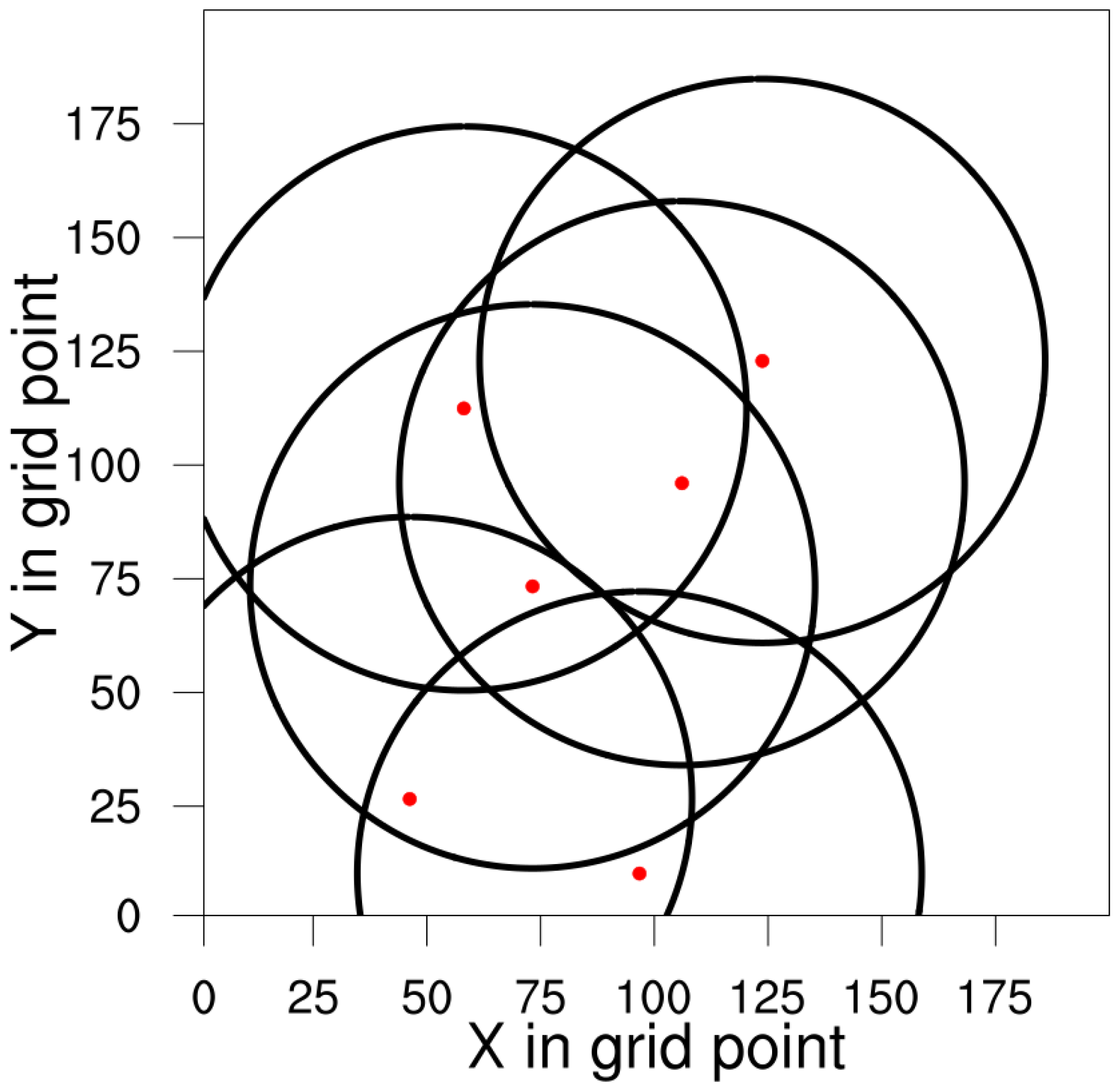
Figure 1 Distribution of the radar network (six radars) expressed by the range of the PPI (plan position indicator) scan at the elevation 0.5^∘.

Figure 2 Nature run: development of the supercell from 13:00 to 18:00 UTC, described by the horizontal wind (vectors; m s⁻¹) at the height of 1 km, the radar reflectivity composite of 0.5^∘ (dotted contour lines for 30 dBZ) and the SDI² (1/s; color shading).

All the prognostic model variables mentioned above are updated. A total of 45 ensemble members are employed, whose initial states differ in the atmospheric profile (i.e., u_∞ and q_v,max) as well as the time and location of the warm bubble (more details can be found in Zeng et al., 2021). Additionally, one deterministic run is initialized by the mean state of the initial ensemble, and the analysis of the deterministic run is computed by applying the Kalman gain for the ensemble mean to the innovation of the deterministic run (Schraff et al., 2016). To maintain sufficient ensemble spread, the method of relaxation to prior perturbations (RTPP; Zhang et al., 2004) is used with a relaxation factor of 0.75 as tuned for the KENDA system (Schraff et al., 2016). The data assimilation cycling period is from 13:00 to 15:00 UTC with the update frequency of 6 min. Ensemble and deterministic forecasts with 3 h of lead time are run starting at 15:00 UTC.

In this work, two twin experiments are conducted, denoted by E_VrZ_6m and E_VrZ_6m_f. The former one is run without the integrated mass-flux adjustment filter (hereafter “filter” for short if not explicitly mentioned), and the latter one is run with the filter.

4 Experimental results

For the investigation of the performance during assimilation cycles, we mainly use the deterministic run instead of the ensemble mean since some small-scale features that we are interested in may be smoothed out in the mean. We calculate the root mean square errors (RMSEs) and spreads, integrated mass-flux divergence, and surface pressure tendency of the background and analysis. Additionally, temperature and moisture deviations in the sub-cloud layer (calculated as deviations of vertical average over 2 km from the horizontal mean, denoted by ΔT and Δq_v, respectively) are used to discuss the structure of cold pools (Seifert and Heus, 2013), and the SDI² is used to compare the ability to reconstruct the mesocyclone of supercells in the analysis, for which the ensemble probabilities from the number of members exceeding a threshold value are computed in a neighborhood manner (Yussouf et al., 2013). To evaluate the forecast skill, grid-point-based ensemble probabilities for the reflectivity composite are provided, and the fractions skill score (FSS; Robert and Lean, 2008) is used. The FSS value varies between 0 and 1, with 1 being a perfect score.

4.1 Assimilation

Figure 3 compares E_VrZ_6m and E_VrZ_6m_f with the nature run in terms of integrated mass-flux divergence and surface pressure tendency fields of the deterministic analysis at 15:00 UTC. Both experiments produce stronger integrated mass-flux divergence fields than the nature run, but E_VrZ_6m_f is considerably better than E_VrZ_6m. Something similar can also be seen for the surface pressure tendency field: the gravity waves are much weaker in E_VrZ_6m_f. It is noticed that the patterns of integrated mass-flux divergence and the surface pressure tendency are comparable in the non-convective regions (this is in line with Eq. 2), and the former one has much stronger signals within the convective regions. Using the same metrics, Fig. 4 further compares the two experiments for the analysis and background at each cycle. It is evident that both result in analyses and backgrounds with larger integrated mass-flux divergence than the nature run, but E_VrZ_6m_f is considerably closer. The surface pressure tendency significantly increases at the analysis step and rapidly decays in the model integration time but does not reach the level of the nature run. E_VrZ_6m_f generates much lower surface pressure tendencies than E_VrZ_6m for both the analysis and background. Overall, it is concluded that the filter effectively reduces the gravity wave noise caused by the data assimilation and thus improves the balance of model states.

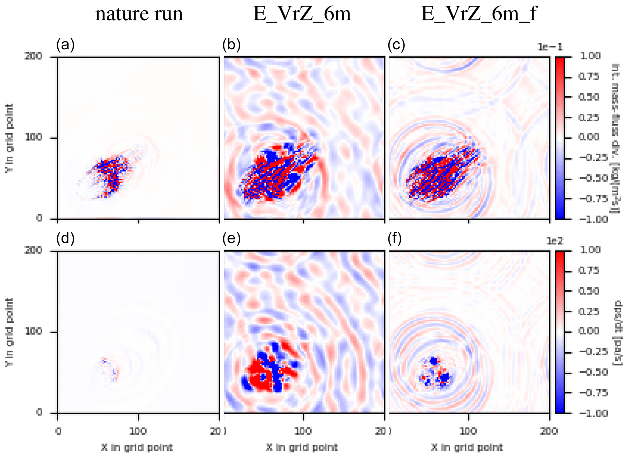
Figure 3 The upper row is for the integrated mass-flux divergence of the nature run (a, d) as well as analyses of E_VrZ_6m (b, e) and E_VrZ_6m_f (c, f) at 15:00 UTC; the second row is for the surface pressure tendency.

Figure 4 Domain-integrated mass-flux divergence of the analysis (indicated by circle) and background at each cycle (a) and domain-averaged surface pressure tendency at the analysis time and at each minute of model integration during the assimilation window (b) for E_VrZ_6m and E_VrZ_6m_f compared with those of the nature run.

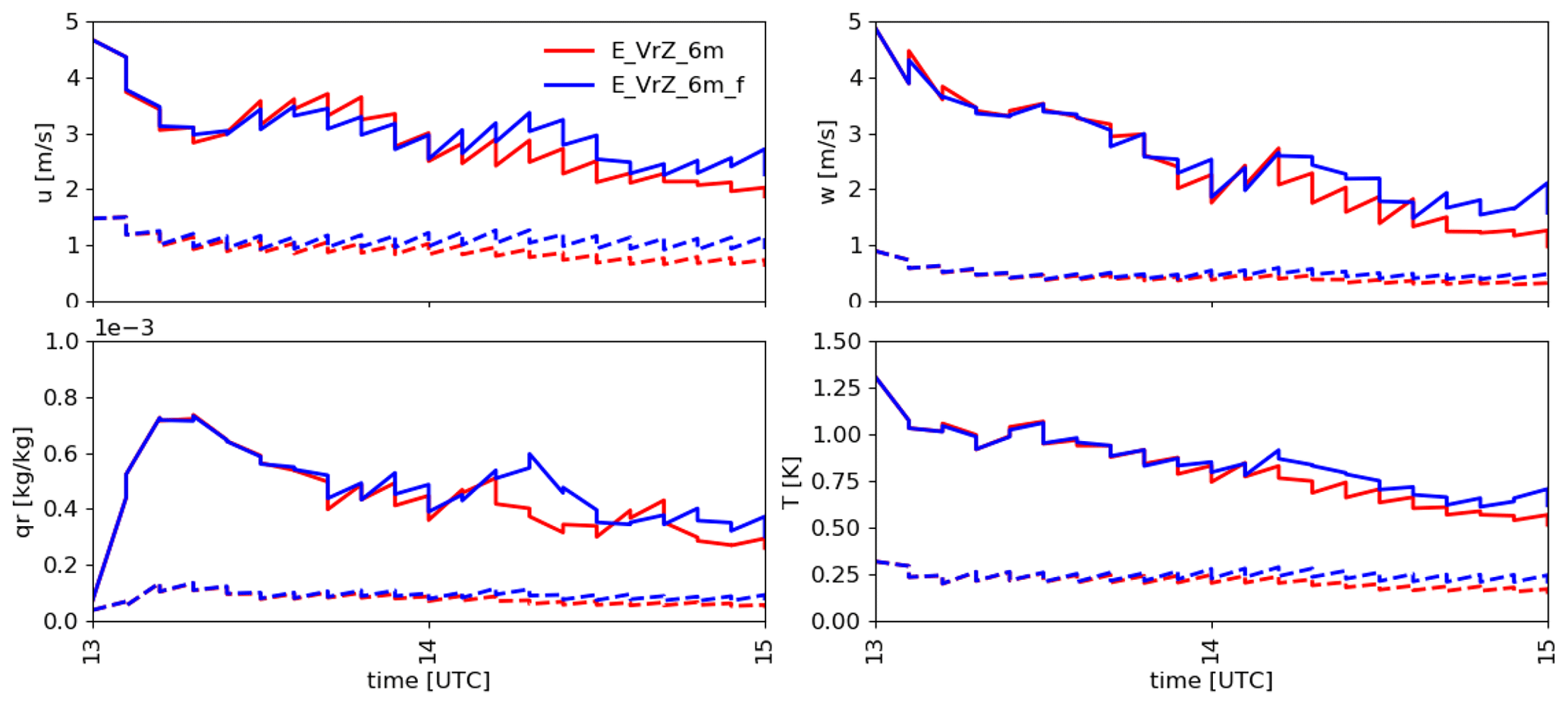
Figure 5 The RMSEs (solid line) and spreads (dashed line) of the deterministic background and analysis (sawtooth pattern) for u, w, q_r and T at each cycle in E_VrZ_6m and E_VrZ_6m_f, averaged over points at which the reflectivity in the nature run is greater than 5 dBZ.

Figure 5 gives the RMSEs and spreads of the deterministic background and analysis for u, w, q_r and T at each cycle. Both E_VrZ_6m and E_VrZ_6m_f exhibit the effectiveness of data assimilation based on decreasing RMSEs, but in general, the former one is associated with slightly smaller RMSEs and spreads for u. This also holds for the other variables. Therefore, the application of the filter causes some loss of analysis accuracy. It is noted that this problem is also often seen by the other filtering methods (e.g., the DFI in Ancell, 2012).

As known, the presence of a cold pool (caused by evaporation of rain and downdrafts) could be important for the development of deep convection (Böing et al., 2012). Figure 6 compares E_VrZ_6m and E_VrZ_6m_f with the nature run in terms of sub-cloud-layer deviations ΔT and Δq_v at 15:00 UTC. The cold pool in E_VrZ_6m is fairly comparable to the truth, although it is generally a bit drier and warmer to different extents in the rear and at some spots on the inside. The cold pool in E_VrZ_6m_f is very similar to that in E_VrZ_6m. Therefore, the cooling and moistening of the sub-cloud layer is reproduced well in both experiments and the filter does not deteriorate the basic structure of the cold pool.

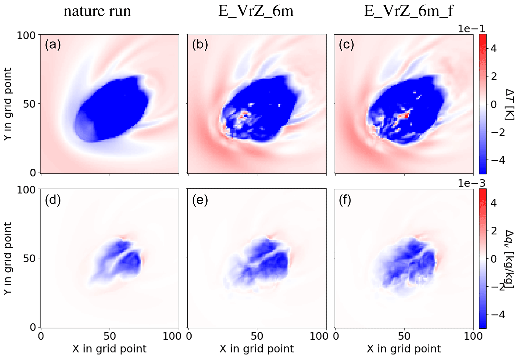
Figure 6 Temperature (a, b, c) and moisture (d, e, f) deviations in the sub-cloud layer for the nature run (a, d) and analyses of E_VrZ_6m (b, e) and E_VrZ_6m_f (c, f) at 15:00 UTC.

In Fig. 7, the SDI² of the deterministic analysis at 15:00 UTC in E_VrZ_6m (left) and E_VrZ_6m_f (right) is given. It is noticed that both experiments capture the major events of mesocyclones well, although some spurious convection exists. For the ensemble probabilities, the good performance of both experiments is also evident; e.g., very high SDI² probabilities (till 100 %) can be seen at locations where SDI²>0.0003 s⁻¹ is present in the nature run, which indicates that the filter preserves the primary characteristics and structures of mesocyclones.

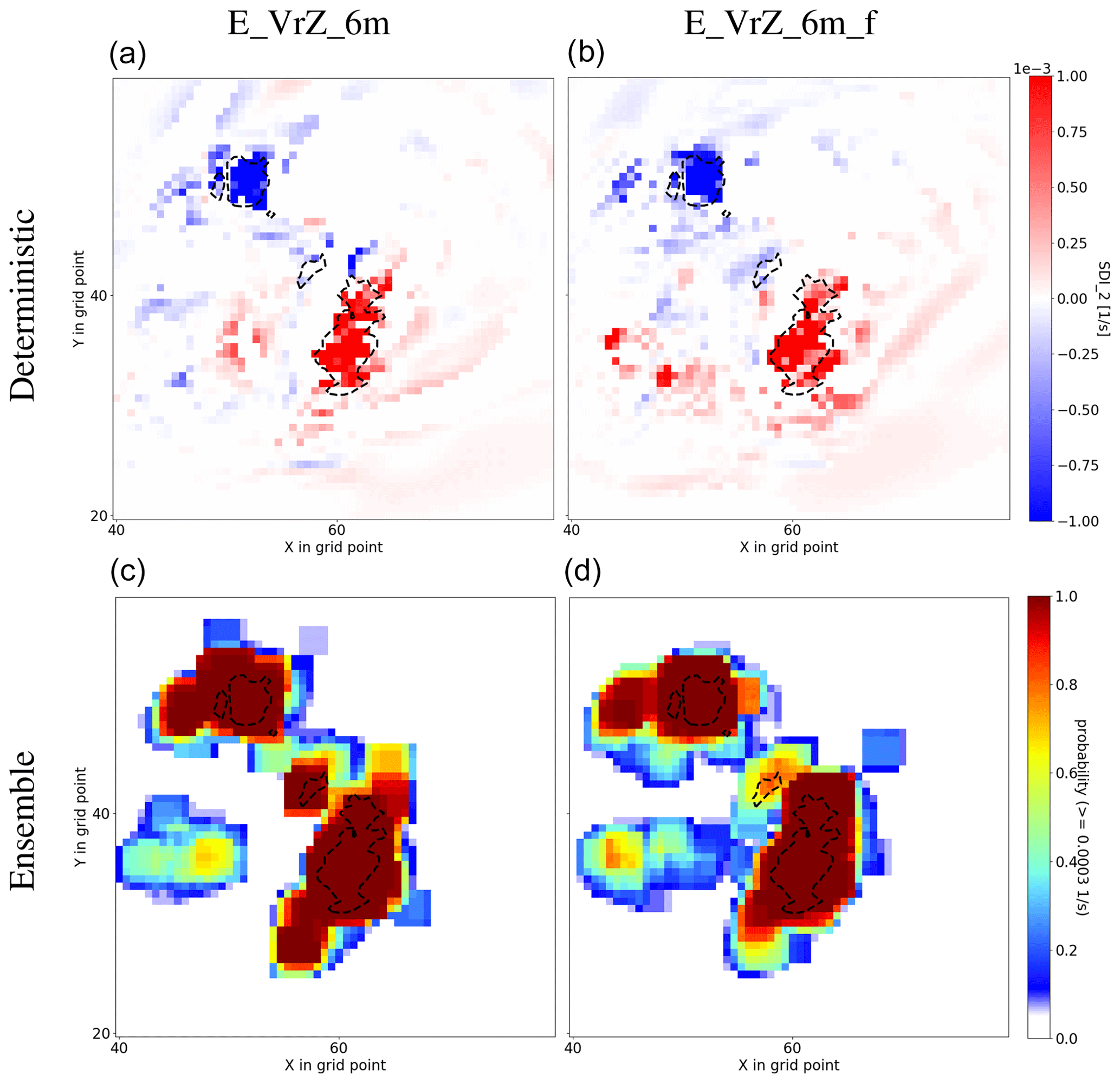
Figure 7 SDI² of the analysis of the deterministic run (a, b) and ensemble (c, d) for E_VrZ_6m (left) and E_VrZ_6m_f (right) at 15:00 UTC. SDI²≥0.0003 s⁻¹ in the nature run is denoted with dashed contour lines. For the ensemble, probabilities exceeding the threshold value of 0.0003 s⁻¹ are calculated using a neighborhood of box length 8 km.

4.2 Forecasting

Figure 8 provides the surface pressure tendency during the 3 h forecast of E_VrZ_6m and E_VrZ_6m_f for the deterministic run. Compared to E_VrZ_6m, the surface pressure tendency of E_VrZ_6m_f is much lower at the initial time, but it somehow increases in the first few minutes, indicating that the filter may introduce some unbalanced modes that are not the solutions of the governing equations of the model and some spin-up time is required, and then it decays rapidly to a steady level close to the nature run in 15 min. Comparatively, the surface pressure tendency of E_VrZ_6m approaches the nature run a bit later in 30 min.

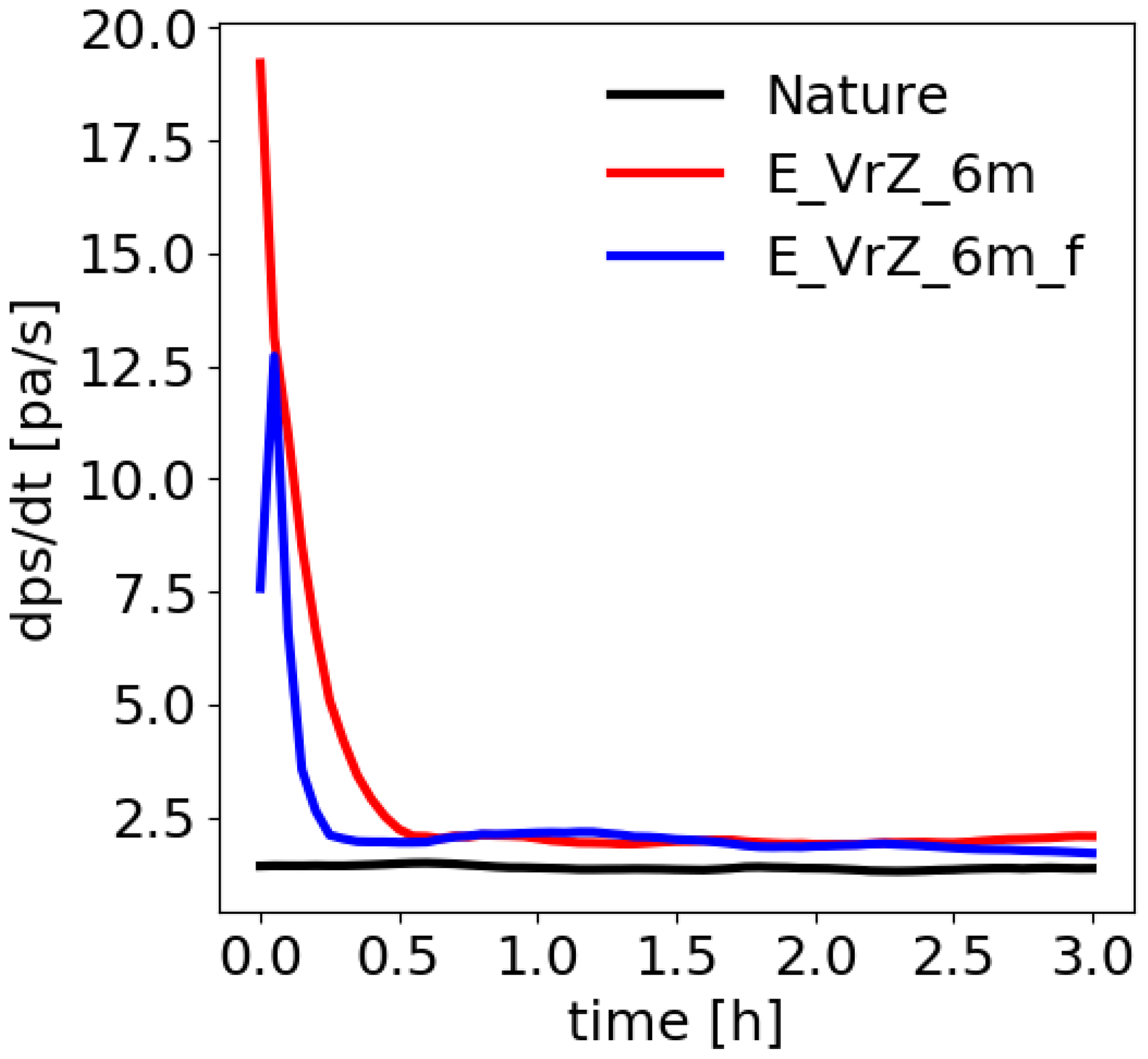
Figure 8 Domain-averaged surface pressure tendency at each minute during the 3 h deterministic forecast starting at 15:00 UTC for the nature run, E_VrZ_6m and E_VrZ_6m_f.

Figure 9 presents deterministic and ensemble forecasts (statistically more robust than the deterministic forecast) by the reflectivity composite at the elevation 0.5^∘. For the deterministic forecast, both E_VrZ_6m and E_VrZ_6m_f represent the storms well but with some spurious convection in the rear; for 1 h of lead time, the right-moving cell is slightly better captured by E_VrZ_6m, but for 2 and 3 h lead times, both cells, especially the right-moving one, are slightly better captured by E_VrZ_6m_f. It is noticed that a considerable amount of spurious convection arises at 3 h of lead time in both experiments. For the ensemble forecast as shown in Fig. 10, both experiments are comparable at the initial time and 1 h of lead time, but for 2 and 3 h lead times, E_VrZ_6m_f outperforms E_VrZ_6m as the former one produces less spurious convection. These results are also confirmed by the FSS in Fig. 11. For the deterministic forecast, E_VrZ_6m is better than E_VrZ_6m_f until 2 h of lead of time, and then E_VrZ_6m_f is better. For the ensemble forecast, E_VrZ_6m_f already becomes superior at 1 h of lead time. Results indicate that the application of the filter reduces the dynamical imbalance of the analyses, which slows down the error growth of model states in free forecasts and thus improves the forecast skills. This is in line with Zeng and Janjić (2016) and Zeng et al. (2017).

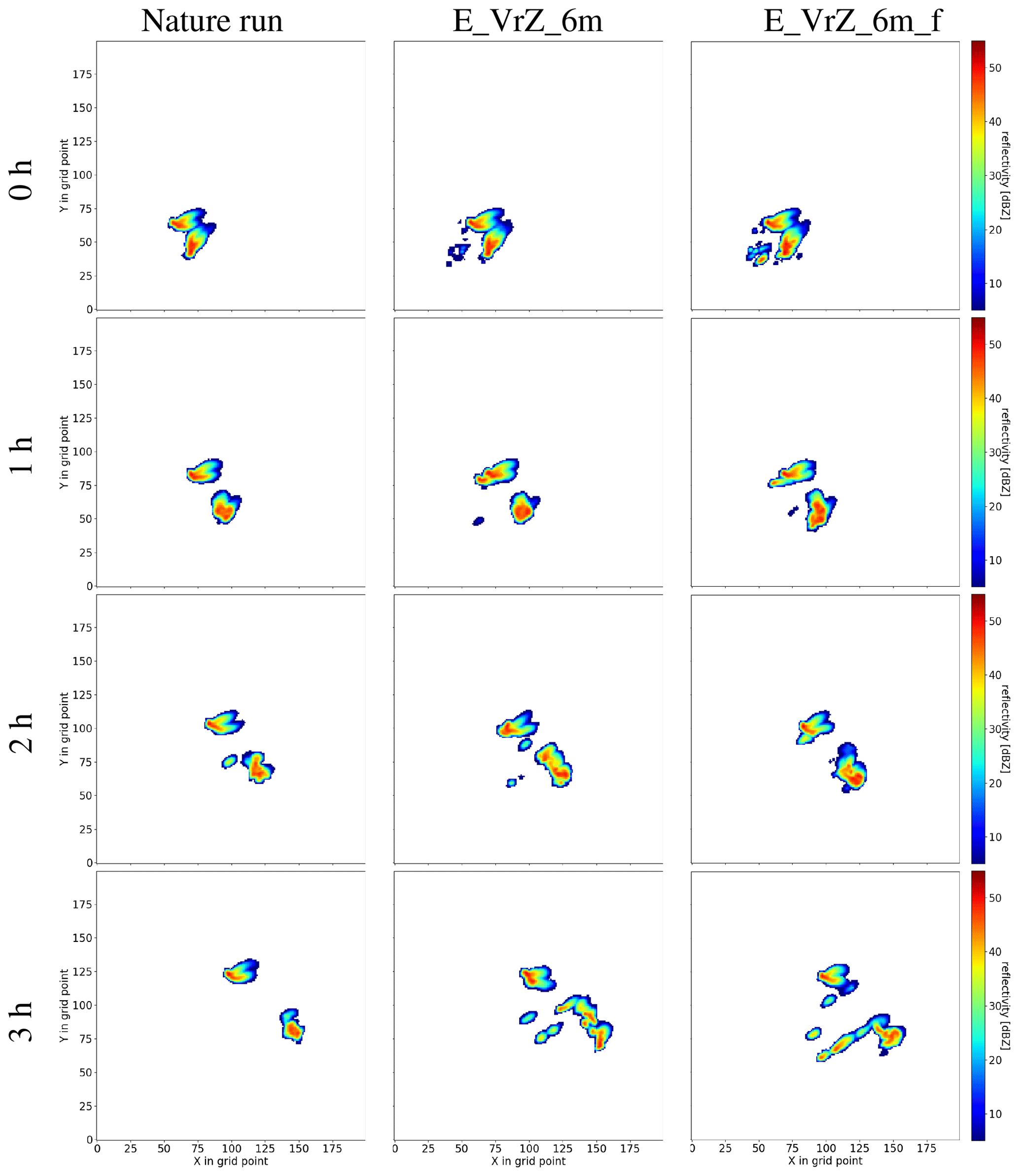
Figure 9 Deterministic forecasts (starting at 15:00 UTC) of E_VrZ_6m (middle) and E_VrZ_6m_f (right) based on the reflectivity composite at the elevation 0.5^∘. The forecasts at the initial times of 1, 2 and 3 h are presented from top to bottom. The left column is the nature run.

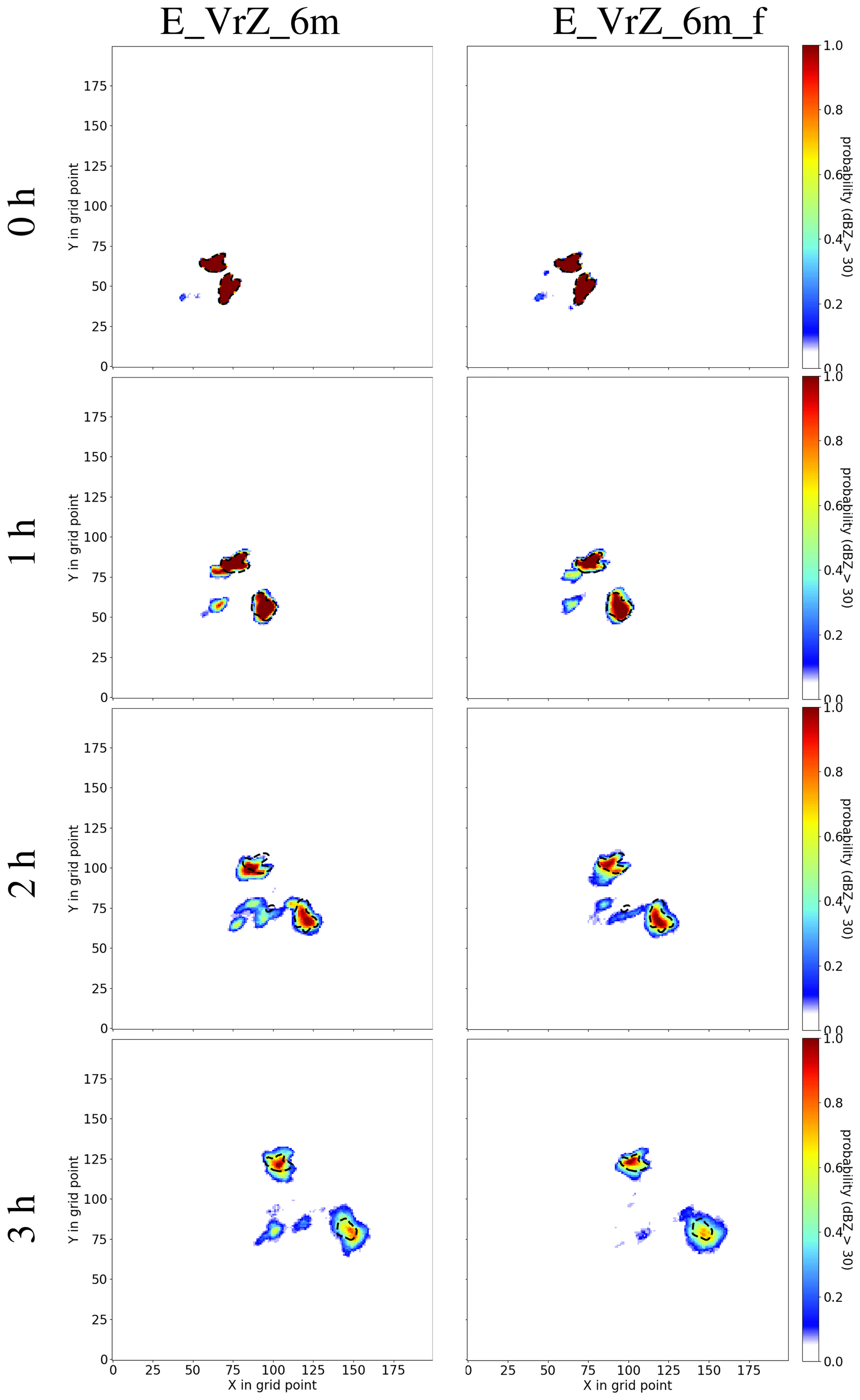
Figure 10 Ensemble forecasts (starting at 15:00 UTC) of E_VrZ_6m (left) and E_VrZ_6m_f (right) based on the grid-point-based probabilities of ensemble members with a reflectivity composite at elevation 0.5^∘ exceeding the threshold value of 30 dBZ. Reflectivity ≥30 dBZ in the nature run is denoted with dashed contour lines. The forecasts at the initial times of 1, 2 and 3 h are presented from top to bottom.

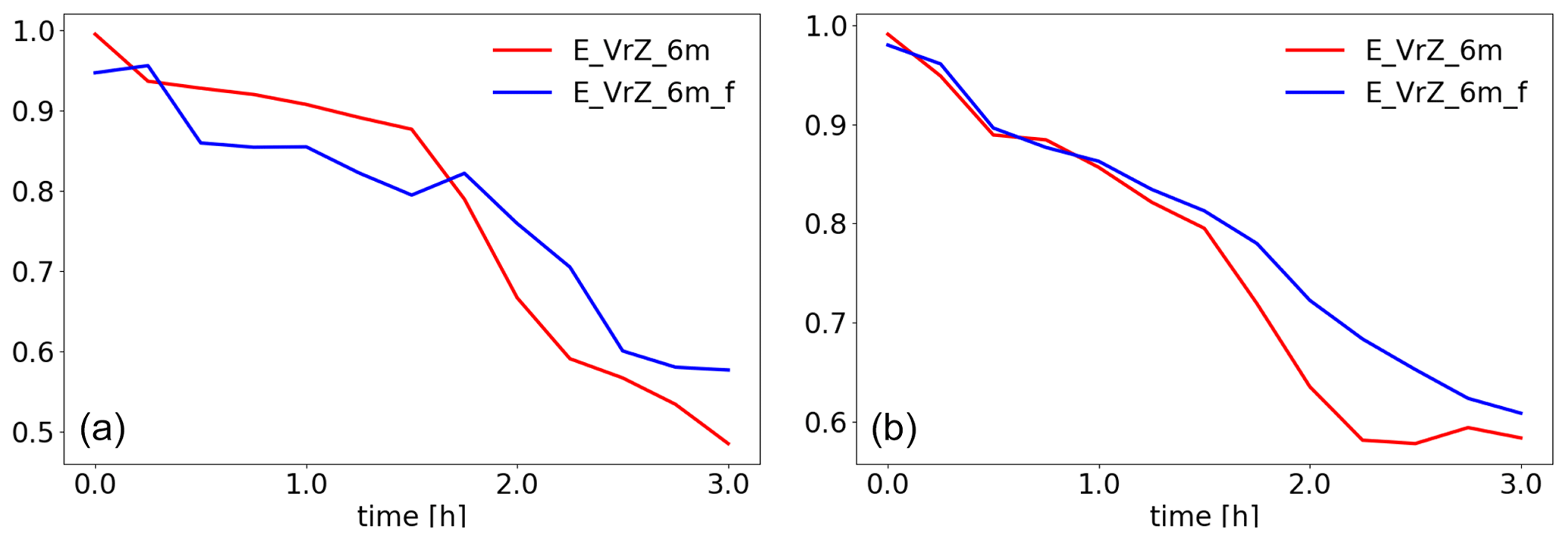
Figure 11 The FSS values of the deterministic (a) and ensemble forecasts (b) starting at 15:00 UTC in E_VrZ_6m and E_VrZ_6m_f based on the reflectivity composite at 0.5^∘ with the threshold value of 30 dBZ and box lengths of 16 km as a function of the forecast lead time up to 3 h (with 15 min outputs). The FSS values of ensemble forecasts are averaged over ensemble members.

5 Summary and outlook

A new integrated mass-flux adjustment filter that uses the analyzed integrated mass-flux divergence field to correct the analyzed wind field has been introduced in this work. The filter has been examined in twin experiments with rapid update cycling (i.e., 6 min) using an idealized setup for convective-scale radar data assimilation. It is found that the new filter slightly reduces the accuracy of background and analysis states; however, it preserves the main structure of cold pools (described by temperature and moisture deviations in the sub-cloud layer) and primary mesocyclone properties of supercells (described the supercell section index). More importantly, it considerably diminishes spurious integrated mass-flux divergence and successfully suppresses the increase in the surface pressure tendency in the analysis. For the ensuing 3 h forecasts, the one that employs the filter becomes more skillful after 1 h. Overall, the filter is a promising tool to alleviate the imbalance problem usually caused by data assimilation.

As seen, the model requires some spin-up time after the application of the filter; this can be attributed to the fact that the filter is currently based on the 2D integrated mass-flux field and the adjustments in the vertical are distributed by a predefined function. In further development, it is reasonable to extend the filter to 3D to get rid of the distribution function; i.e., the wind is corrected by analyzed mass flux at each level individually, which may result in even more balanced wind fields. Furthermore, the filter is a post-processing approach that does not consider the accuracy of model states while reducing the imbalance. An idea that takes both of these aspects into account is to impose the filter as a weak constraint to the cost function of EnKF algorithms. Finally, although the filter has been tested here for convective-scale data assimilation with rapid cycling, it can also be useful for lower update frequencies and synoptic-scale data assimilation. This is worth exploring in the future, as is its applicability in nonidealized data assimilation.

Appendix A

The Helmholtz–Hodge decomposition says that any vector field tangent to the surface of the sphere can be written as the sum

$$\begin{array}{}\text{(A1)}& \mathit{f}={\mathrm{\nabla }}_{\mathrm{H}}\mathit{\varphi }+{\mathrm{\nabla }}_{\mathrm{H}}\times \mathit{\psi },\end{array}$$

where ϕ and ψ are scalar potential functions. In this work, $\mathit{f}={\mathit{M}}_{\mathrm{a}}^{u,v*}$.

Because the divergence of a curl is zero, we obtain the Poisson equation:

$$\begin{array}{}\text{(A2)}& {\mathrm{\nabla }}_{\mathrm{H}}{\mathit{M}}_{\mathrm{a}}^{u,v*}={\mathrm{\nabla }}_{\mathrm{H}}\cdot {\mathrm{\nabla }}_{\mathrm{H}}\mathit{\varphi }={\mathrm{\nabla }}_{\mathrm{H}}^{\mathrm{2}}\mathit{\varphi }.\end{array}$$

Due to Eq. (3), it holds that

$$\begin{array}{}\text{(A3)}& {\mathrm{\nabla }}_{\mathrm{H}}^{\mathrm{2}}\mathit{\varphi }={\mathrm{\nabla }}_{\mathrm{H}}{\mathit{M}}_{\mathrm{a}}.\end{array}$$

Solving the Poisson equation (Eq. A3), we obtain ϕ.

Because the vorticity of a gradient field is zero, we obtain the Poisson equation,

$$\begin{array}{}\text{(A4)}& {\mathrm{\nabla }}_{\mathrm{H}}^{\mathrm{2}}\mathit{\psi }={\mathrm{\nabla }}_{\mathrm{H}}\times {\mathit{M}}_{\mathrm{a}},\end{array}$$

in an analogous way. Solving Eq. (A4), we obtain ψ.

Finally, substituting ϕ and ψ in Eq. (A1), we obtain ${\mathit{M}}_{\mathrm{a}}^{u,v*}$.