Reconstructing climatic modes of variability from proxy records using ClimIndRec version 1.0

Modes of climate variability strongly impact our climate and thus human society. Nevertheless, the statistical properties of these modes remain poorly known due to the short time frame of instrumental measurements. Reconstructing these modes further back in time using statistical learning methods applied to proxy records is useful for improving our understanding of their behaviour. For doing so, several statistical methods exist, among which principal component regression is one of the most widely used in paleoclimatology. Here, we provide the software ClimIndRec to the climate community; it is based on four regression methods (principal component regression, PCR; partial least squares, PLS; elastic net, Enet; random forest, RF) and cross-validation (CV) algorithms, and enables the systematic reconstruction of a given climate index. A prerequisite is that there are proxy records in the database that overlap in time with its observed variations. The relative efficiency of the methods can vary, according to the statistical properties of the mode and the proxy records used. Here, we assess the sensitivity to the reconstruction technique. ClimIndRec is modular as it allows different inputs like the proxy database or the regression method. As an example, it is here applied to the reconstruction of the North Atlantic Oscillation by using the PAGES 2k database. In order to identify the most reliable reconstruction among those given by the different methods, we use the modularity of ClimIndRec to investigate the sensitivity of the methodological setup to other properties such as the number and the nature of the proxy records used as predictors or the targeted reconstruction period. We obtain the best reconstruction of the North Atlantic Oscillation (NAO) using the random forest approach. It shows significant correlation with former reconstructions, but exhibits higher validation scores.

1 Introduction

The interdependent components of the climate system, such as the atmosphere and the ocean, vary at different timescales. The interactions between those components (Mitchell et al., 1966) lead the climate to vary from the hourly to the multidecadal timescales. Preindustrial control simulations of global coupled climate models have evidenced that such a variability is still present without any modulation of the external forcings, which is frequently referred to as internal variability (Hawkins and Sutton, 2009). External factors such as volcanic aerosols (Mignot et al., 2011; Swingedouw et al., 2015; Khodri et al., 2017), anthropogenic aerosols (Evan et al., 2009, 2011; Booth et al., 2012), solar irradiance (Swingedouw et al., 2011; Seidenglanz et al., 2012) and greenhouse gas concentrations (Stocker et al., 2013) also influence the variations and dynamics of the climate system by altering the Earth's radiation balance. By only considering the impact of external forcings which are not due to human activity, we can characterized the so-called natural climate variability.

An unequivocal synchronous rise in both the greenhouse gas concentration in the atmosphere and the global mean temperature has been observed in instrumental measurements (Stocker et al., 2013). However for temperatures, fluctuations around this trend from one decade to another (Kosaka and Xie, 2013; Santer et al., 2014; Swingedouw et al., 2017) highlight the modulating role of natural variability at decadal to multidecadal scales. Improving our knowledge about past natural climate variability and its sources is therefore essential to better understand the potential coming changes in climate.

Physics driving the climate system induce large-scale variations, organized around recurring climate patterns with specific regional impacts and temporal properties. These variations are known as climate modes of variability. Their evolution is usually quantified by an index that can be calculated from a specific observed climate variable. These indices provide an evaluation of the corresponding climate variations and their regional impacts (Hurrell, 1995; Neelin et al., 1998; Trenberth and Shea, 2006). As an example, the North Atlantic Oscillation (NAO) is the leading mode of atmospheric variability in the North Atlantic basin (Hurrell et al., 2003). Generally defined as the sea level pressure (SLP) gradient between the Azores High and the Icelandic Low, the NAO describes large-scale changes of winter atmospheric circulation in the Northern Hemisphere and controls the strength and direction of westerly winds and storm tracks across the Atlantic (Hurrell, 1995). A stronger than normal SLP gradient between the two centres of action induces a northward shift of the eddy-driven jet stream. Such large scale changes in atmospheric circulation lead to precipitation and temperature variations in various regions (North Africa, Eurasia, North America and Greenland; Casado et al., 2013). Moreover, these meteorological impacts have major influences on many ecological processes, including marine biology (Drinkwater et al., 2003) and terrestrial ecosystems (Mysterud et al., 2001). This mode also affects the oceanic convection in the Labrador Sea and the Greenland, Iceland and Norwegian seas through changes in atmospheric heat, freshwater and momentum fluxes (Dickson et al., 1996; Visbeck et al., 2003). These changes may lead in turn to modifications in the Atlantic Meridional Overturning Circulation (AMOC) which then affect poleward heat transport and the related sea surface temperature (SST) pattern over the Atlantic (Trenberth and Fasullo, 2017).

The dynamics of these modes are still not fully understood due to the relatively short duration of the instrumental records, which prevents robust statistical evaluation of their properties (e.g. spectrum, stability of teleconnections, underlying mechanisms). To partly overcome this limitation, reconstructions of climate beyond the period of direct measurements have been performed in numerous studies that combine appropriate statistical methods and information from proxy records. Proxy records provide indirect estimates of past local or regional climate, derived from natural archives coming for instance from sediment cores, speleothems, ice cores or tree rings. According to its nature, each proxy record has a specific temporal resolution, from years to millennia, and can cover a specific period: from hundreds to millions of years. New proxy records are continuously gathered, extending the available datasets and allowing paleoclimatologists to build increasingly consistent reconstructions (PAGES 2K Consortium, 2013, 2017).

Based on the assumption that climate modes such as the NAO affect climate conditions in different locations, some studies have used regression-based methods on temperature and drought-sensitive proxy records to reconstruct the variability of these modes over the last thousand years. Luterbacher et al. (2001) first proposed a partly monthly and seasonal reconstruction of the NAO that extends back to 1500 using the principal component regression (Hotelling, 1957) (PCR) method. Another study reconstructed the SLP fields in Europe covering the same time frame using a PCR approach as well (Luterbacher et al., 2002), and found consistencies with the Luterbacher et al. (2001) NAO reconstruction. Cook et al. (2002) also proposed a complete methodology of nested PCR using annually resolved proxy records bounding the North Atlantic to reconstruct the NAO variability further back to 1400. More recently, Ortega et al. (2015) performed a NAO reconstruction from 1073 to 1969, also based on the PCR, using 48 proxy records that were significantly correlated with the historical NAO index over their common time window. Instead of nesting reconstructions of different sizes, which can lead to inhomogeneities between time windows using different proxy selections, this study used several random calibration/validation samplings of the overlap period of the NAO index and the proxy records to perform individual reconstructions on the same time frame. Regression-based methods have also been used for reconstructing climate modes indices other than NAO, such as for instance El Niño–Southern Oscillation index (Li et al., 2013) and the Atlantic Multidecadal Variability index (Gray et al., 2004; Wang et al., 2017).

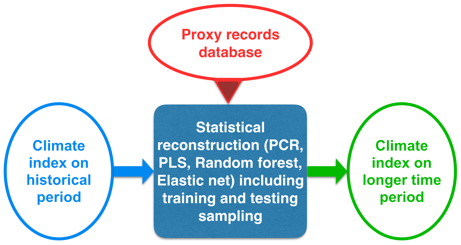
More recent algorithms than PCR provide alternative regression methods that can also be used to reconstruct climate modes, and may possibly further improve the quality and the robustness of these reconstructions. In this paper, we present the computer tool ClimIndRec (Climate Index Reconstruction) version 1.0, which includes multiple statistical approaches, for reconstructing climate modes indices. It is based on four regression methods: PCR (Hotelling, 1957), partial least squares (PLS; Wold et al., 1984), elastic net (Enet; Zou and Hastie, 2005) and random forest (RF; Breiman, 2001). It communicates with a large proxy database that contains various types of proxy records distributed worldwide, which are sensitive to different climate variables. ClimIndRec is thus designed to reconstruct the past variability of different climate modes (Fig. 1). It should be stressed that ClimIndRec will only be useful with climate indices for which there are enough proxy records representing their regional climate imprints, and that have the appropriate time resolution to capture their preferred timescale of variability. Besides the climate modes, ClimIndRec can also be used to reconstruct other kinds of climate time series such as temperature or precipitation in a given location.

Figure 1 Scheme summarizing the main features of ClimIndRec.

Section 2 develops the functioning and the added-value of ClimIndRec for climate time series reconstruction. Section 3 compares the four regression methods by reconstructing the NAO index over the last millennium and investigates the reconstruction sensitivity to methodological choices such as the method used, the learning period or the proxy records selection for regression. Finally, Sect. 4 presents a discussion including some outlooks for the next version of ClimIndRec and the conclusions of this study.

2 Data, notation and methodologies

2.1 General methodology of ClimIndRec

We here compare four models that all consist of regression methods among which the PCR has been used in many paleoclimate studies (Luterbacher et al., 2001, 2002; Cook et al., 2002; Gray et al., 2004; Ortega et al., 2015; Wang et al., 2017). The methods we added (PLS, Enet and RF) aim at exploring alternative approaches to PCR and comparing different reconstructions using relevant metrics. PLS is a similar approach to PCR, where the difference is that the matrix of empirical orthogonal functions (EOFs) is calculated by maximizing the variance of the projected proxies on the EOFs and the targeted climate index instead of the variance of the projected proxies (Wold et al., 1984). Enet belongs to the regularized regression method family not usually used in paleoclimate reconstructions (Zou and Hastie, 2005). It is here investigated in order to find out if this kind of regression approach is relevant for climate index reconstruction. Finally, the RF method is an aggregation of multiple predictors called “regression trees”, which are non-linear regression approaches (Breiman, 2001). The mathematical details for each method are elaborated in Sect. S1 in the Supplement. Given a climate index and proxies, ClimIndRec optimizes a given regression method with cross-validation-based techniques and can thus be extrapolated to other regression-based approaches. Hence, updates of ClimIndRec will be dedicated to propose other regression methods such as adaptive lasso regression (Zou, 2006).

In the case of the reconstruction of climate indices, regression methods seek to establish for each common time step the relationships between the proxies and the climate index to be reconstructed over the period of instrumental measurements. This set of relationships constitutes a statistical model of the considered climate index. The paleo-variations of proxy records are then translated into a climate index in the past using the relationships previously established by the statistical model. Since they all use unknown parameters, they must be optimized to make the reconstruction as robust as possible. In the case of PCR, for example, the number of principal components of the proxies used to regress the climate index directly affects the reconstruction since it modifies the set of predictors. The term “control parameter” is used to design this ensemble of parameters inherent to each method. They are identified for each method in Sect. S1. Their tuning (or optimization) using cross-validation techniques (Stone, 1974; Geisser, 1975) are elaborated later in this section.

Reconstruction of the same climate index obtained from different regression methods may significantly differ. Thus, if the same index is reconstructed using different regression methods that each suggest different interpretations of the past, it may be difficult to compare them directly. A common approach is to separate the observation years (called learning period) in two to evaluate a statistical model. The first period, called the training (or calibration) period, is used to build the model using control parameter tuning, and thus to establish relationships between the climate index and proxies. The proxies of the second period, called the testing (or validation) sample, are then translated into a climate index over the years of observations of this period. The actual values of the climate index can then be compared with the reconstructed climate index over the testing period using a given metric which will be defined in Sect. 2.3.2. It gives a score estimating the model ability to reconstruct the climate index using the first-seen data of proxies. This procedure is called the “hold-out” approach (McCornack, 1959).

The scores obtained for different regression methods for a given training/testing sample might be impacted by the specific sampling. This is overcome by repeating the hold-out approach several times where years of observations between the training and the testing samples are shuffled. An ensemble of scores is obtained, yielding an evaluation of the methods' ability to reconstruct the climate index. The most robust regression model is the one that has the highest scores, as it means this is the most accurate at reconstructing the climate index using the first-seen data of proxies. This most robust regression method is then applied to the whole learning period to build a final model and infer the paleo-variations of the climate index from proxy records. In our study, and by default in ClimIndRec, the determination of the testing samples is performed using a block-style approach over time. This means that the first testing period of a given size encompasses the first time steps of the learning period. This testing period is then shifted by one time step which gives the second testing period of same size, and so on until each time step of the learning period has been used at least once for testing. The reason is that for climate time series, autocorrelation is often large, so that one obtains skills from persistence alone. Thus sampling is usually used with a block-style approach for climate time series.

The reconstruction might also largely differ for a same reconstruction method according to both the proxy records used and the years of observations used. Here, the sources of uncertainties associated with the proxy selection as well as the learning period used can be reduced using the same hold-out approach with evaluation and comparison of optimal sets using scores.

The number of proxy records and the reconstruction period are thus fixed for the different training/testing period sections and the final model, in contrast with some previous studies which used nested approaches (Cook et al., 2002; Wang et al., 2017). We make this choice because the aim of this study is mainly focused on optimizing the methodological approach for the reconstruction and not the reconstruction itself. Nevertheless, ClimIndRec can be used to perform reconstructions on different time windows which can then be aggregated to perform a nested reconstruction, with associated scores for each portion of time.

It should be stressed that the approach of ClimIndRec implicitly assumes that the climate index to be reconstructed is a linear combination of the proxy records. It means assuming that the climate reacts to proxies, while the correct etiological relationship is the other way around (Tingley et al., 2012). Hence, it has to be specified that since climate variations affect proxies variations, we can attempt to estimate past climate fluctuations using statistical methods. Another caveat to highlight is that the proxy records used have their own uncertainties that can come from various sources such as measurement methodologies, dating uncertainties or transfer function used to infer paleoclimate variations from bio/geochemical data. This inevitably leads to an underestimation of the true link between the climate index and the climate variable associated with the proxy record and therefore leads to a biased reconstruction with loss of variance (Isobe et al., 1990). To overcome this issue, previous climate index reconstruction studies (Ortega et al., 2015; Wang et al., 2017) rescaled the variance of the reconstruction according to the observed climate index variance. However it implies that the variance of the climate index is stationary, which might not be true. In this study we thus present the raw reconstructions and the loss of variance will be quantified and specified.

ClimIndRec has been developed using both bash and R scripts. It uses different R packages (presented Table S5 in the Supplement) that can be used independently to blindly perform reconstructions of any climate index. The added-value of ClimIndRec is to integrate the synchronous hold-out approach and cross-validation according to the user inputs (proxy records, regression method, reconstruction period targeted, proxy records pre-selection). It therefore allows several inputs to be tested and provides relevant metrics that can be used to determine the optimal regression model.

2.2 Step-by-step procedure for reconstruction and model evaluation

The general reconstruction and model evaluation procedure follows 12 steps (Fig. 1), applied sequentially as follows:

1. An observational time series representing modulations of the targeted mode of variability is chosen to be used as the predictand.

2. A target time period 𝒯 for the reconstruction is selected.

3. The statistical reconstruction method to be applied is selected.

4. The proxy records that overlap with the selected reconstruction period are extracted to be used as predictors.

5. The common period T between the observed climate index and the selected proxy records is identified and extracted for evaluating the reconstruction method.

6. This common period is split in two, one for training the model (training period), and one for testing it (testing period). This is repeated R times following a block-style approach to perform splits, R depending on the size of the learning period and the size of testing periods determined by the user.

7. The proxy records that have a significant correlation at a given threshold with the climate index over the training period are selected to train the statistical model.

8. Each of the R sets of periods and proxies is calibrated over the training window for all the different sets of control parameters of the given method selected in (3), and the best performing one is identified.

9. The corresponding optimal setup is then applied to extend the reconstruction over the testing period for each member.

10. Validation scores are computed by comparing each of the observation-based testing series and each training sample-based individual reconstruction over the corresponding testing period.

11. The corresponding control parameters are tuned over the whole learning period T and the final model is built.

12. The final reconstruction is obtained by applying the final model to the proxies over the reconstruction period 𝒯.

Thus ClimIndRec provides the final reconstruction with associated uncertainties (Sect. S3) and a vector with R validation scores following different metrics as final outputs.

2.3 Model evaluation and optimization

This section aims to clarify the technical details of the methodology presented in Sect. 2.1 and 2.2. It will thus call on the elements mentioned above.

2.3.1 Data notation

To simplify the mathematical notation, we make the assumption that the proxy record selection and truncation to their common time window with the climate index have already been undertaken (see Sect. 2.2, steps 4 and 5). In this study, it is important that all proxy records are truncated to the same time window to make them mergeable in the same matrix. Each record has to cover at least the chosen reconstruction time window 𝒯 and it is excluded otherwise (Sect. 2.2, step 2). Hence, the proxy records matrix does not contain missing values.

Figure 2 illustrates how the proxy data are organized in the input matrix X. We denote ${\mathbf{X}}^{\mathrm{1}}=({\mathbf{X}}_t^{\mathrm{1}}{)}_{t\in \mathcal{T}},\mathrm{\dots },{\mathbf{X}}^p=({\mathbf{X}}_t^p{)}_{t\in \mathcal{T}}$, where t stands for the time (with N annual time steps), and p is the number of proxy records on the same period 𝒯. X is thus an N×p matrix grouping the individual records: $\mathbf{X}=[{\mathbf{X}}^{\mathrm{1}},\mathrm{\dots },{\mathbf{X}}^p]$. $\mathit{Y}=({\mathit{Y}}_t{)}_{t\in T}$ is the target climate index, defined on the historical time window T called the learning period, that contains n annual time steps. The period where Y is not known is denoted τ, containing m annual time steps (Fig. 2). Thus $\mathcal{T}=T\cup \mathit{\tau }$ is the entire reconstruction period, which contains $N=n+m$ annual time steps. With these notations, the dimensions of the different matrices and vectors are $\mathbf{X}\in {\mathbb{R}}^{N\times p}$; ${\mathbf{X}}_{\left(T\right)}\in {\mathbb{R}}^{n\times p}$; ${\mathbf{X}}_{\left(\mathit{\tau }\right)}\in {\mathbb{R}}^{m\times p}$; Y∈ℝⁿ. The learning set is denoted {X_(T),Y}, and the reconstruction set is denoted {X_(𝒯)}.

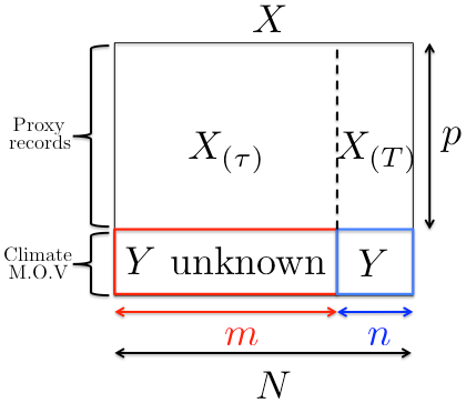
Figure 2 Scheme of the initial data. X and Y are respectively the proxy records matrix and the index of the considered mode of variability. N is the size of the common period of all proxy records. n is the size of the common period of all proxy records and the index of the mode of variability. m is the size of the common period of all proxy records, where the mode of variability is not known. p is the number of proxy records. X_(T) is the sub-matrix of X where the mode of variability is known. X_(τ) is the sub-matrix of X where the mode of variability is not known.

2.3.2 Terms and validation metrics

We denote the chosen reconstruction method by ℳ. Each method is defined by a specific number of control parameters q, contained in the vector denoted θ. We can denote the function ℳ as a function of (i) a set on which the model is built ({X,Y}), (ii) observations of the predictors on the reconstruction period (X_(rec)) and (iii) an control parameter vector (θ):

$$\begin{array}{}\text{(1)}& {\displaystyle }\mathcal{M}:(\left\{\mathbf{X},\mathit{Y}\right\},{\mathbf{X}}_{\left(\mathrm{rec}\right)},\mathit{\theta })\to {\widehat{\mathit{Y}}}_{\mathit{\theta }},\text{(2)}& {\displaystyle }\begin{array}{rl}& (\left\{{\mathbb{R}}^{n\times p},{\mathbb{R}}^n\right\},{\mathbb{R}}^{m\times p},{\mathbb{R}}^s)\to {\mathbb{R}}^m\\ & n,p,m,s\in \mathbb{N}\left(\text{not fixed}\right).\end{array}\end{array}$$

Hence, the ℳ function gives an entire reconstruction of size m∈ℕ, depending on θ.

We introduce S as the score function, or validation metric. This function is an indicator that estimates the quality of a reconstruction $\widehat{\mathit{Y}}$ with respect to the observed values Y_(obs):

$$\begin{array}{}\text{(3)}& {\displaystyle }& {\displaystyle }S:({\mathit{Y}}_{\left(\mathrm{obs}\right)},\widehat{\mathit{Y}})\to s,\text{(4)}& {\displaystyle }& {\displaystyle }({\mathbb{R}}^m,{\mathbb{R}}^m)\to \mathbb{R}.\end{array}$$

In this paper, three kind of validation metrics are used for different tasks. The first is a correlation function, the second is a root mean squared error (RMSE) function and the third is the Nash–Sutcliffe coefficient of efficiency (Nash and Sutcliffe, 1970):

$$\begin{array}{}\text{(5)}& {\displaystyle }{S}_{\mathrm{cor}}({\mathit{Y}}_{\left(\mathrm{obs}\right)},\widehat{\mathit{Y}})=\text{Cor}({\mathit{Y}}_{\left(\mathrm{obs}\right)},\widehat{\mathit{Y}}),\text{(6)}& {\displaystyle }{S}_{\mathrm{RMSE}}({\mathit{Y}}_{\left(\mathrm{obs}\right)},\widehat{\mathit{Y}})=\Vert {\mathit{Y}}_{\left(\mathrm{obs}\right)}-\widehat{\mathit{Y}}\Vert =\sqrt{\sum _{i=\mathrm{1}}^m({\mathit{Y}}_{i\left(\text{obs}\right)}-{\widehat{\mathit{Y}}}_i{)}^{\mathrm{2}}},\text{(7)}& {\displaystyle }\begin{array}{rl}& S_{\mathrm{NSCE}}({\mathit{Y}}_{\left(\mathrm{obs}\right)},\widehat{\mathit{Y}})=\mathrm{1}-{\displaystyle \frac{{\sum }_{i=\mathrm{1}}^m({\mathit{Y}}_{i\left(\text{obs}\right)}-{\widehat{\mathit{Y}}}_i{)}^{\mathrm{2}}}{{\sum }_{i=\mathrm{1}}^m({\mathit{Y}}_{i\left(\mathrm{obs}\right)}-{\stackrel{\mathrm{‾}}{\mathit{Y}}}_{\left(\mathrm{obs}\right)}{)}^{\mathrm{2}}}},\\ & \mathrm{\text{with}}{\stackrel{\mathrm{‾}}{\mathit{Y}}}_{\left(\mathrm{obs}\right)}={\displaystyle \frac{\mathrm{1}}{m}}\sum _{i=\mathrm{1}}^m{\mathit{Y}}_{i\left(\mathrm{obs}\right)}.\end{array}\end{array}$$

S_NSCE is used to validate the reconstruction methods over the testing period, and S_RMSE allows one to determine the optimal control parameters (θ) for the reconstruction. We use S_cor because it is used in the last NAO reconstruction of Ortega et al. (2015), with which we will compare our results. S_NSCE is a metric defined as being between −∞ and 1, where values lower than 0 mean that using the mean over the training period is better than the proposed statistical model (Nash and Sutcliffe, 1970); additional information about this metric is presented in Sect. S2. Here, we will consider that a final reconstruction is robust and reliable when its R NSCE scores are significantly positive at the 99 % confidence level using the Student test. As the possible values of the NSCE score is not symmetric around 0, the best reconstruction is identified as the one that has a higher median of NSCE scores.

2.3.3 Control parameter tuning by cross-validation and final reconstruction

As mentioned above, the initial learning sample is split into R partitions of two subsets: $\left\{T_{\left(\mathrm{train}\right)}^{\left(r\right)},T_{\left(\mathrm{test}\right)}^{\left(r\right)}\right\}$, $\forall \mathrm{1}\le r\le R$ (Sect. 2.2, step 6). For a given method ℳ, R reconstructions are build on the R training samples. $\forall \mathrm{1}\le r\le R$; we denote $\left\{{\mathbf{X}}_{\left(\mathrm{train}\right)}^{\left(r\right)},{\mathit{Y}}_{\left(\mathrm{train}\right)}^{\left(r\right)}\right\}$ as the training set, and $\left\{{\mathbf{X}}_{\left(\mathrm{test}\right)}^{\left(r\right)},{\mathit{Y}}_{\left(\mathrm{test}\right)}^{\left(r\right)}\right\}$ as the test set. At each step, the columns of X, X_(train) and X_(test) are normalized to the mean and the standard deviation of the respective columns of X_(train).

To estimate the optimal set of control parameters θ_opt on a given training set {X_(train),Y_(train)}, we use the K-fold cross-validation (CV) approach (KFCV; Sect. 2.2, steps 8 and 9; Stone, 1974; Geisser, 1975). Cross-validation methods, are in general, widely used as parametrization and model validation techniques (Kohavi, 1995; Browne, 2000; Homrighausen and McDonald, 2014; Zhang and Yang, 2015). Here, it is used as an optimization method to empirically determine an optimal set of control parameters for θ. As presented in Fig. 3, the KFCV splits the observations into a partition of K groups of same sizes (or approximately same sizes if the length of the training set is not divisible by K). $\forall \mathrm{1}\le k\le K$, we denote {X_(k),Y_(k)}, containing only information for the kth drawn sample. Then, $\left\{{\mathbf{X}}_{(-k)},{\mathit{Y}}_{(-k)}\right\}$ is the set containing all the K−1 other sets. For all possible values of θ contained in Θ, we scan the K models based on the sets s ${\left\{{\mathbf{X}}_{(-k)},{\mathit{Y}}_{(-k}\right\}}_{\mathrm{1}\le k\le K}$. The empirical optimal set of control parameters is obtained by minimizing the averaged S_RMSE functions on the K splits by considering all possible combinations of θ (Stone, 1974). Mathematically, the optimal KFCV set of control parameters θ_KF is determined by

$$\begin{array}{}\text{(8)}& \begin{array}{rl}{\mathit{\theta }}_{\mathrm{KF}}& =\arg \underset{\mathit{\theta }\in \mathrm{\Theta }}{min}{\displaystyle \frac{\mathrm{1}}{K}}\sum _{k=\mathrm{1}}^K{S}_{\mathrm{RMSE}}\\ & ({\mathit{Y}}_{\left(k\right)},\mathcal{M}(\left\{{\mathbf{X}}_{(-k)},{\mathit{Y}}_{(-k)}\right\},{\mathbf{X}}_{\left(k\right)},\mathit{\theta }\left)\right).\end{array}\end{array}$$

It should be noted that if dim(θ)>1, then the different control parameters need to be optimized simultaneously, with nested KFCVs.

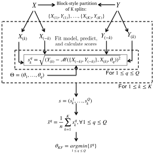
Figure 3 Scheme of a K-fold cross-validation procedure to select the optimal control parameter of a specific learning method ℳ. X is the input set of predictors and Y the corresponding variability mode index. $\forall \mathrm{1}\le i\le n$, {X_(k),Y_(k)} is the kth block-style-based group of observation and $\mathit{\{}{\mathbf{X}}_{(-k)},{\mathit{Y}}_{(-k)}\mathit{\}}$ contains all observations except the ith. $\mathrm{\Theta }=({\mathit{\theta }}_{\mathrm{1}},\mathrm{\dots },{\mathit{\theta }}_Q)$ is the ensemble of possible values of the s control parameters θ∈ℝ^s.

Using this approach, we retain the control parameter vector ${\widehat{\mathit{\theta }}}_{\mathrm{opt}}={\mathit{\theta }}_{\mathrm{KF}}$ for the given method ℳ and a given learning set {X,Y}. KFCV is applied to build a unique optimized reconstruction for every training sets and any given method. Then, for all the corresponding and independent testing periods, the associated testing series ${\mathit{Y}}_{\left(\mathrm{test}\right)}^{\left(r\right)}$ are compared to the individual reconstructions using the S_NSCE function. This way, R NSCE scores are obtained for ℳ. In Sect. 3, the distributions of the NSCE scores will be used as a metric to compare different reconstructions. Figure 4 shows the calculations that gives the NSCE scores for a given method ℳ.

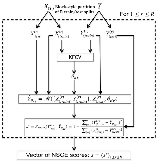
Figure 4 Scheme of the whole procedure for score calculation for a given method ℳ. Y is the index of the chosen mode of variability. X_(T) is the proxy dataset restricted to the period where Y known. $\mathit{\{}{\mathbf{X}}_{\left(\mathrm{train}\right)}^{\left(r\right)},{\mathit{Y}}_{\left(\mathrm{train}\right)}^{\left(r\right)}\mathit{\}}$ is the rth training sample and $\mathit{\{}{\mathbf{X}}_{\left(\mathrm{test}\right)}^{\left(r\right)},{\mathit{Y}}_{\left(\mathrm{test}\right)}^{\left(r\right)}\mathit{\}}$ is the rth testing sample. θ_KF is the empirically optimal set of parameters obtained by applying the KFCV (Fig. 3; Sect. 2.3.3).

It should be stressed that K-fold cross-validation sampling is also implemented following a block-style approach in ClimIndRec for the same reasons than for the hold-out approach. This means that the K groups of observations are constructed along time instead of being randomly split. Also, the choice of K can have implications for the estimation of optimal control parameters. A large K leads to more diverse training samples, thereby bringing more variable estimates of RMSE. On the other hand, a small K leads to a low number of samples used, thereby increasing the bias due to the particular way splits have been made. Additional works have shown that this choice poorly influences the final reconstruction obtained (not shown) so that we decided to set it to K=5 for this study. It is set at K=5 by default in ClimIndRec but it can certainly be changed in order to produce alternative reconstructions.

Once the model has been evaluated, it is launched over the whole learning set {X_(T),Y} with a K-fold cross-validation to optimize the control parameters such as done previously for training samples.

2.4 Data

The assessment of the proposed reconstruction techniques is investigated for the NAO index, as it is probably the mode of variability that has been observed for the longest time period. This index is indeed relatively simple to calculate from the SLP time series as it only requires two locations with instrumental records: one within the centre of action of the Azores anticyclone (typically Gibraltar) and one within the Icelandic Low (typically Reykjavik). The reference NAO index is then calculated as the normalized SLP difference between these two locations. We here use the Jones et al. (1997) index spanning the whole historical period since 1856.

In terms of proxies, we use the state-of-the-art PAGES 2k database (PAGES 2K Consortium, 2017) in its latest 2017 version (hereafter P2k2017). Proxy records with resolutions lower than annual were removed. Even if these proxy records could be interpolated to a finer temporal scale and used for the reconstruction, their use is not recommended as the interpolated time series will present high auto-correlation coefficients, which could inflate the correlations with the NAO and thus their weight in the final reconstruction, potentially leading to spurious results (Hanhijarvi et al., 2013). We added 44 annually resolved proxy records used in Ortega et al. (2015) and not present in P2k2017 (see Table S1). We end up with a database of 554 well-verified and worldwide-distributed annually resolved proxy records.

3 Results

3.1 Methodological sources of uncertainty in the reconstruction

We apply ClimIndRec with the four methods presented above to the reconstruction of the NAO. In the following, each reconstruction is obtained by averaging R individual reconstructions performed for R training/testing splits. R depends on the size of the testing samples relative to the size of the learning period as we perform block-style splits of the data to produce training and testing samples (Sect. 2.1 and 2.2). Here, we set the relative length of the training splits as 80 % of the learning period. NSCE scores are thus produced and stored in a vector of R elements. This vector will thus be used as a quality metric to characterize the methodological uncertainty in the reconstruction. The following actions were undertaken to minimize the reconstruction uncertainty identified in Sect. 2.1, and estimate its sensitivity:

1. pre-selecting the most relevant proxy records,

2. selecting the best learning period.

These two steps are described below, before assessing the reconstruction itself.

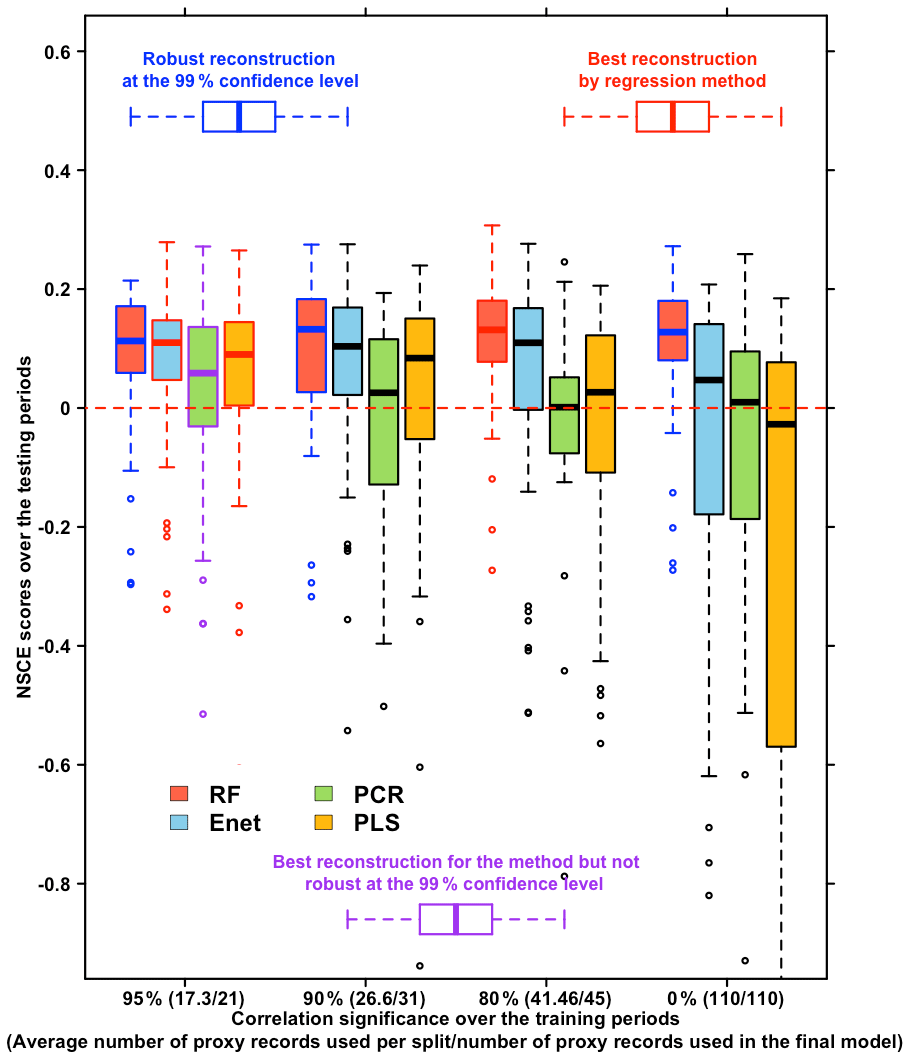
Figure 5 Boxplot of NSCE scores obtained for the four methods and different groups of proxy records by reconstructing the NAO index of the period 1000–1970 with R=50 training/testing samples. Green boxplots are the NSCE scores obtained for the PCR method. Yellow boxplots are the NSCE scores obtained for the PLS method. Red boxplots are the NSCE scores obtained for the RF method. Blue boxplots are the NSCE scores obtained for the Enet method. The first cluster of boxplots is the NSCE scores obtained by using all the available proxy records over the period (110 proxy records). The second cluster of boxplots is the NSCE scores obtained by using only proxy records significantly correlated with the NAO index at the 80 % confidence level over the training periods. The third cluster of boxplots is the NSCE scores obtained by using only proxy records significantly correlated with the NAO index at the 90 % confidence level over the training periods. The fourth cluster of boxplots is the NSCE scores obtained by using only proxy records significantly correlated with the NAO index at the 95 % confidence level over the training periods. Boxplots with blue edges are the scores significantly positive at the 99 % confidence level. Boxplots with red edges correspond to the scores associated with the best reconstruction for each method.

3.1.1 Proxy pre-selection

Among the previous climate reconstruction studies, Ortega et al. (2015) performed a proxy selection over the training periods at the 90 % confidence level using the correlation test from McCarthy et al. (2015) while Cook et al. (2002) and Wang et al. (2017) selected their proxies by focusing on the regions affected by the modes they respectively reconstructed. Here we run four reconstructions of R=50 individual members for each method. These reconstructions are respectively performed with different significance levels for the proxy selection by correlation over the training periods. These levels are 0 % (which means that all the records are used at each training/testing split), 80 %, 90 % and 95 %. The reconstructions are performed for the reconstruction period $\mathcal{T}=\left[\right[\mathrm{1000},\mathrm{1970}\left]\right]$ and the learning period $\mathcal{T}=\left[\right[\mathrm{1856},\mathrm{1970}\left]\right]$ encompassing 110 available proxy records with n=115.

Figure 5 shows that RF method, particularly useful for larger datasets, is more efficient using the proxy records correlated at the 80 % confidence level with med(S_NSCE)=0.15 (med is the median function), even if using proxy records uncorrelated with the NAO or not located in regions affected by NAO variations. On the other hand, the three other regression methods are more adapted when the finest proxy selection (95 %) is applied, as highlighted by Ortega et al. (2015) for the PCR. Figure 5 also evidences that the widely used PCR method and PLS have to be employed cautiously with a statistically based proxy selection over the training periods in further studies. Indeed the reconstructions performed with these methods are only significantly robust at the 99 % confidence level (see Sect. 2.3.2) by using any pre-selection of proxies. Conversely, for the RF and Enet methods, the proxy selection does not affect the statistical robustness of the reconstruction, with reconstructions significantly robust at the 99 % confidence level (see Sect. 2.3.2) for every choice of proxy selection.

Overall, RF gives the best NSCE scores. Nevertheless, it should be stressed that these results have been obtained for a particular learning period (1856–1970). The sensitivity to this is assessed in the next section.

3.1.2 Sensitivity to the learning period

In this section, we keep for each method the optimal selection of proxy records over the training periods (see Sect. 3.1.1). We explore the impact of the reconstruction period. This affects the final reconstruction in two different ways, both related to the final proxy selection, as explained in Sect. 2.1.

We run the reconstruction for 31 periods 𝒯: from 1000–1970 to 1000–2000, with an increment of 1 year. By doing so, the number of available proxy records is not the same for each of the periods (see Fig. 6). Figure 6a shows the NSCE scores obtained for the different reconstruction/learning periods. Using the NSCE metric, we find that the best reconstruction time window is 1000–1972 for PLS and RF methods and 1000–1971 for Enet and PCR methods.

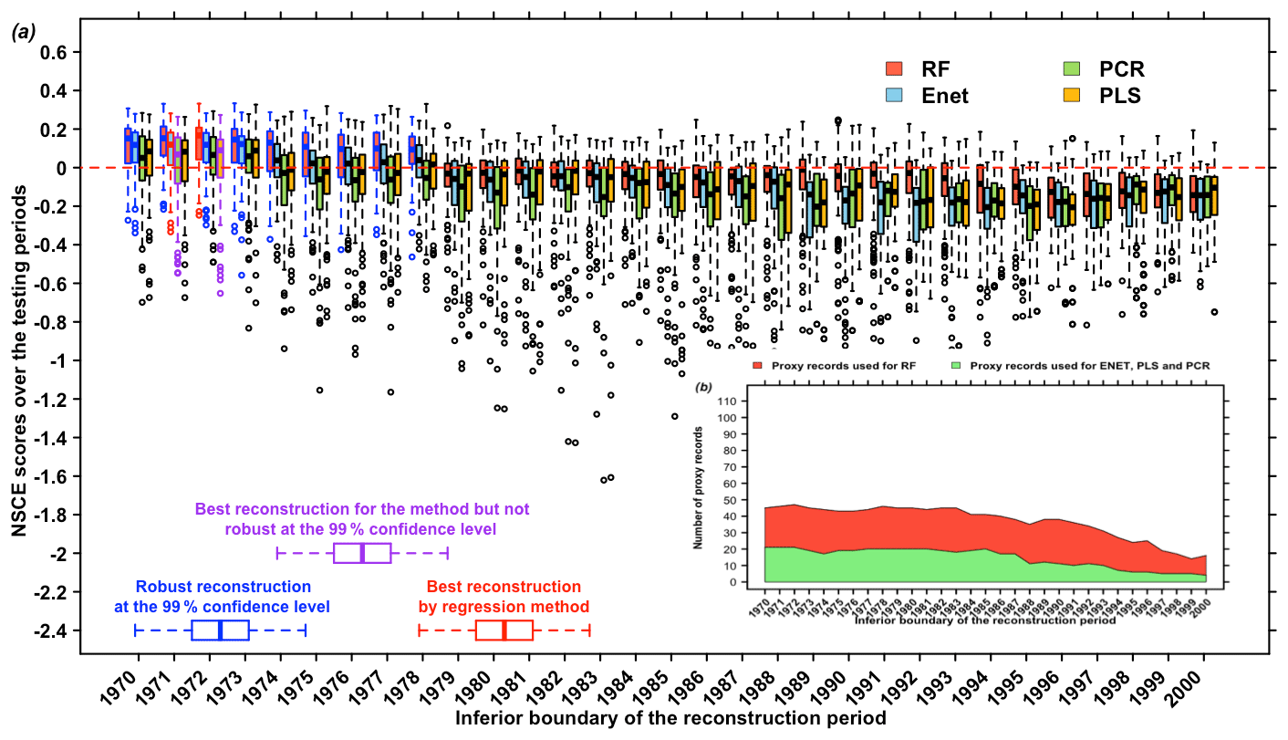
Figure 6 (a) Reconstructions are performed using 31 reconstruction periods for the four methods: from 1000–1970 to 1000–2000 by moving the most recent year by 1 with R=50 training/testing samples. RF reconstructions are performed using the proxy records significantly correlated at the 80 % confidence level with the NAO over the training periods (Sect. 3.1.1). PCR reconstructions are performed by selecting the proxy records significantly correlated at the 95 % confidence level with the NAO over the training periods (Sect. 3.1.1). PLS and Enet reconstructions are performed by selecting the proxy records significantly correlated at the 95 % confidence level with the NAO over the training periods (Sect. 3.1.1). (a) Red boxplots are the NSCE scores obtained using the RF method. Blue boxplots are the NSCE scores obtained using the Enet method. Red green are the NSCE scores obtained using the PCR method. Yellow boxplots are the NSCE scores obtained using the PLS method. Boxplots with blue edges are the significantly positive scores at the 99 % confidence level. Boxplots with red edges correspond to the scores associated with the best reconstruction for each method. (b) Proxy records available/used by reconstruction period. The red area shows the number of records used for RF. The green area shows number of records used for Enet, PCR and PLS for each reconstruction period.

Following the optimal setup for each method from Sect. 3.1.1, RF uses 47 records and the three others use 21 records (Fig. 6b). Among these four optimized reconstructions, which are the final ones of this study, the RF gives the highest NSCE scores with med(S_NSCE)≃0.16 and $S_{\mathrm{NSCE}}\in [-\mathrm{0.4},\mathrm{0.4}]$ (Fig. 6a).

Results show that the four methods are strongly affected by the choice of the reconstruction period. Thus, we recommend determining this period carefully with different simulations in different time windows, following the approach we presented here, easily performable using ClimIndRec. Overall, this study shows that for each optimization, PCR and PLS are less reliable to reconstruct the NAO than RF and Enet (Sect. 3.1.1 and this section).

3.2 Scientific results

We compare and investigate the reconstruction with highest scores for each method following Sect. 3.1. The four optimized reconstructions are obtained by using the full set of proxy records for RF and only using the proxy records significantly correlated at the 95 % confidence level with the NAO index over the learning period for the other methods (see Sect. 3.1.1). RF and Enet reconstructions are performed for the period 1000–1972 while PCR and PLS reconstructions are performed for the period 1000–1970 (Sect. 3.1.2).

3.2.1 Comparison with previous work

Figure 7 shows the different reconstructions of the NAO, including the Ortega et al. (2015) calibration-constrained reconstruction (only proxy-based), and Table 1 exhibits the paired correlations between the five reconstructions. The regression uncertainties (see Sect. S3) are also shown for the four reconstructions of this study in Fig. 7. The normality of the residuals for the four methods has been verified for both the models built over the training samples and the final model as demonstrated in Fig. 9. Table 1 and Fig. 7 shows that the NAO reconstruction based on RF is distinguishable from the four others including Ortega et al. (2015). Indeed its correlation with the other indices ranges between 0.49 and 0.67 (Table 1) while the paired correlations obtained between the others are greater than 0.88. Additionally Fig. 8 shows that the RF reconstruction has a higher correlation with the Jones et al. (1997) NAO index than the other indices: r=0.98 (p<0.01), while the Ortega et al. (2015) reconstruction has a correlation of 0.45 (p<0.01). The RF reconstruction that uses 46 proxy records (22 common proxies with Ortega et al. (2015) presented in Fig. 10) has the best NSCE scores ($\text{med}\left(S_{\mathrm{NSCE}}\right)=\mathrm{0.16};S_{\mathrm{NSCE}}\in [-\mathrm{0.24},\mathrm{0.33}]$; Sect. 3.1.1) and its correlation scores ($\text{med}\left(S_{\mathrm{cor}}\right)\simeq \mathrm{0.43};S_{\mathrm{cor}}\in [\mathrm{0.06},\mathrm{0.63}]$) are significantly higher at the 99 % confidence level than the Ortega et al. (2015) calibration-constrained reconstruction ($S_{\mathrm{cor}}\in [-\mathrm{0.14};\mathrm{0.58}];\text{med}\left(S_{\mathrm{cor}}\right)\simeq \mathrm{0.24}$) and model-constrained reconstruction ($S_{\mathrm{cor}}\in [\mathrm{0.14};\mathrm{0.64}];\text{med}\left(S_{\mathrm{cor}}\right)\simeq \mathrm{0.43}$). We thus statistically verified that the best reconstruction from this study is more robust and reliable than those from Ortega et al. (2015). This improvement in performance may arise from the inclusion of new relevant proxy records into the reconstruction, but also from the use of a new statistical regression method for climate index reconstruction: the RF. Finally, it has to be stressed that the five reconstructions presented in Fig. 7, including Ortega et al. (2015), do not show a predominant positive NAO phase during the Medieval Climate Anomaly, contrary to the hypothesis formulated by Trouet et al. (2009).

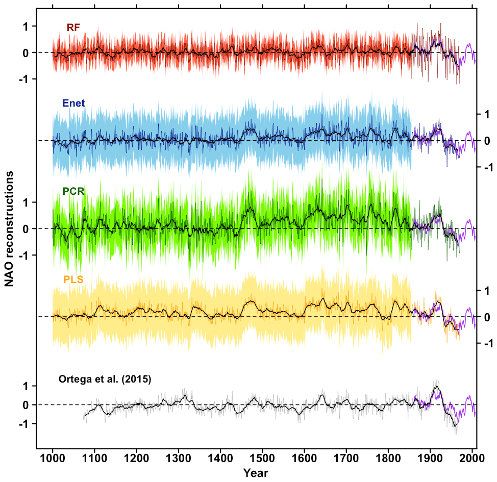
Figure 7 Red line: RF reconstruction for the period 1000–1972 (Sect. 3.1.2), using proxy records significantly correlated at the 80 % confidence level with the NAO over the training periods (Sect. 3.1.1). Blue line: Enet reconstruction for the period 1000–1971 (Sect. 3.1.2) by selecting the proxy records significantly correlated with the NAO index at the 95 % confidence level over the training periods (Sect. 3.1.1). Green line: PCR reconstruction for the period 1000–1971 (Sect. 3.1.2) by selecting the proxy records significantly correlated with the NAO index at the 95 % confidence level over the training periods (Sect. 3.1.1). Orange line: PLS reconstruction for the period 1000–1972 (Sect. 3.1.2) by selecting the proxy records significantly correlated with the NAO index at the 95 % confidence level over the training periods (Sect. 3.1.1). Thin black line: calibration-constrained reconstruction (Ortega et al., 2015). Red area: regression uncertainties (see Sect. S3) for the RF reconstruction. Blue area: regression uncertainties for the Enet reconstruction. Blue area: regression uncertainties for the PCR reconstruction. Orange area: regression uncertainties for the PLS reconstruction. Thick black lines are the corresponding 11-year filtered reconstructions for each method. Purple lines: superposed 11-year filtered NAO index from Jones et al. (1997).

Table 1 Table of correlations between five reconstructions: Ortega et al. (2015) reconstruction; RF reconstruction for the period 1000–1972 using the proxy records significantly correlated with the NAO at the 80 % confidence level; Enet reconstruction for the period 1000–1972 only using the proxy records significantly correlated with the 95 % confidence level; PCR reconstruction for the period 1000–1970 only using the proxy records significantly correlated with the NAO at the 95 % confidence level; PLS reconstruction for the period 1000–1970 only using the proxy records significantly correlated with the NAO at the 95 % confidence level.

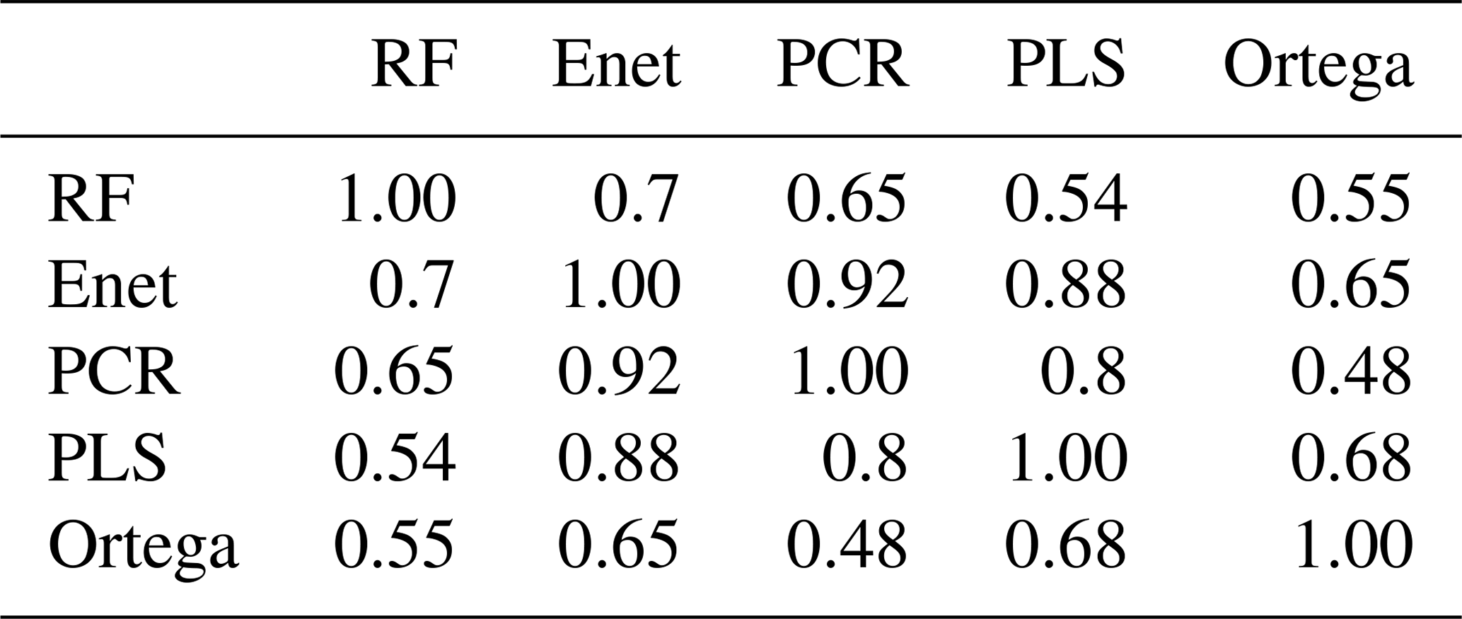
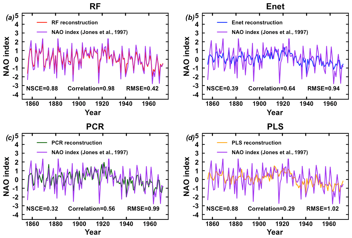
Figure 8 Comparison of reconstructions from this study with the original Jones et al. (1997) NAO index (purple line) over their common period. (a) RF reconstruction. (b) Enet reconstruction. (c) PCR reconstruction. (d) PLS reconstruction. NSCE, RMSE and correlation statistics are provided.

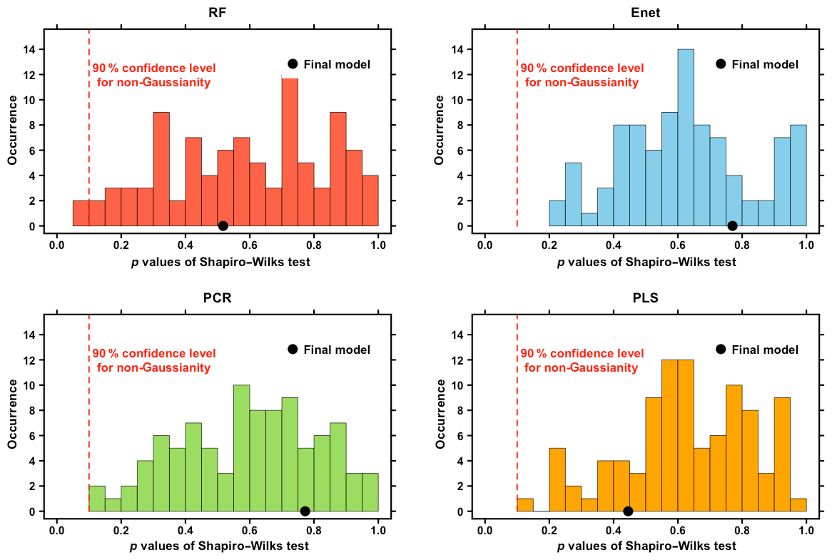
Figure 9 P values obtained from Shapiro–Wilk normality tests on the residuals from each reconstruction of Fig. 7. For panels (a) RF, (b) Enet, (c) PCR and (d) PLS, the repartition of the 50 p values obtained for each training/testing split is presented. Red dashed lines indicate the 90 % confidence level for non-normality. For $\mathrm{0}\le \mathit{\alpha }\le \mathrm{1}$, if the p value ≤α, it means that the residual distribution is significantly non-Gaussian at the 1−α confidence level (see shapiro.test R documentation). Black dots indicate the p values of the residuals obtained for the final models.

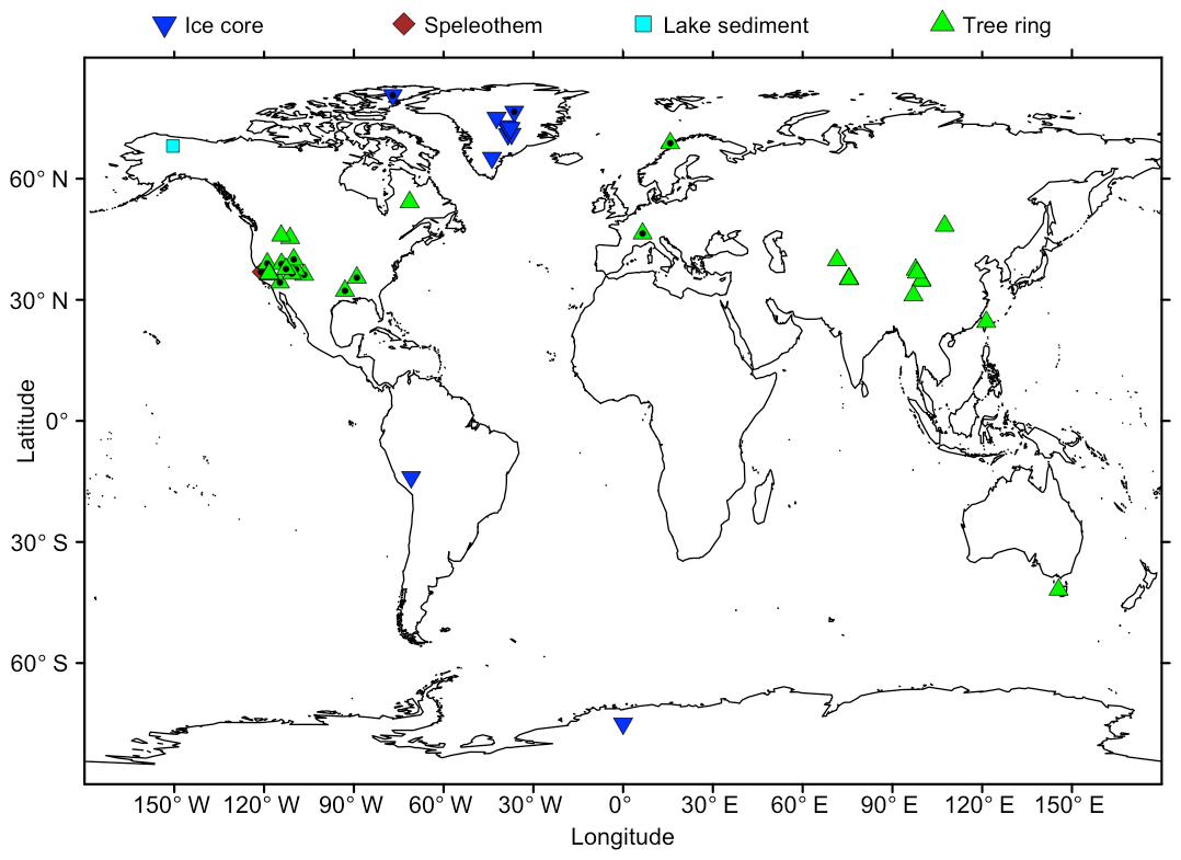
Figure 10 Map of the 46 proxy records used for the reconstruction of the NAO index from Jones et al. (1997) over the time window 1000–1972 using the RF method. Points with a black dot are proxy records also used in Ortega et al. (2015).

3.2.2 Response to external forcing

No significant correlation is found between the NAO reconstruction based on RF method and the total solar irradiance (TSI) reconstruction from Vieira et al. (2011) ($r\simeq -\mathrm{0.11};p>\mathrm{0.18}$). The same is true for the best reconstruction of the other methods (not shown) and Ortega et al. (2015). None of the reconstructions (including Ortega et al., 2015) show clear negative phases during the Maunder and the Spörer minima as suggested by some model simulations (Shindell et al., 2004). In addition, no significant correlation on the pre-industrial era has been found with the CO₂ reconstruction based on a Law Dome (East Antarctica) ice core (Etheridge et al., 1996) (not shown), indicating that the NAO is not linearly associated with CO₂ variations over this time frame.

Ortega et al. (2015) suggested that a positive NAO phase is triggered 2 years after strong volcanic eruptions, a response that is not reproduced over the last millennium by model simulations (Swingedouw et al., 2017). We use the 10 large volcanic eruptions selected in Ortega et al. (2015) and a second selection (see Table S2) of the 11 largest volcanic eruptions from the well-verified reconstruction of Sigl et al. (2015). By using a superposed epoch analysis and the Rao et al. (2019) Monte Carlo approach to calculate significance (see Sect. S4), we find that using the same set of eruptions as Ortega et al. (2015) leads to the same result: a significant positive response of the NAO 2 years after the eruption. However, for RF this result is not significant with its p value of just under 0.1 (Fig. 11). Conversely, by using the 11 largest volcanic eruptions from Sigl et al. (2015), we find a significant response at the 90 % confidence level for PLS, but 1 year after the eruption with a p value of under 0.05 (Fig. 11). For RF, Enet and PCR, the positive NAO response is significant 1 to 3 years after the eruption (Fig. 11). Here again, the significance for the RF composite is smaller than for the other methods while this reconstruction is associated with the highest NSCE scores. Individual response analysis shows that for the RF reconstruction, this result is particularly significant for the two largest eruptions of the millennium (Samalas, 1257, Kuwae, 1458) and not so clear for the nine others (not shown). This result suggests that the positive NAO response might be mainly associated with volcanic eruptions with very large and rare intensities such as the Samalas or Kuwae eruptions and less connected with eruptions of weaker intensities. However, further studies might be useful to verify the statistical robustness of this result, as this kind of event (eruption at least as strong as Kuwae, 1453) is very rare, thus only providing two events for this study.

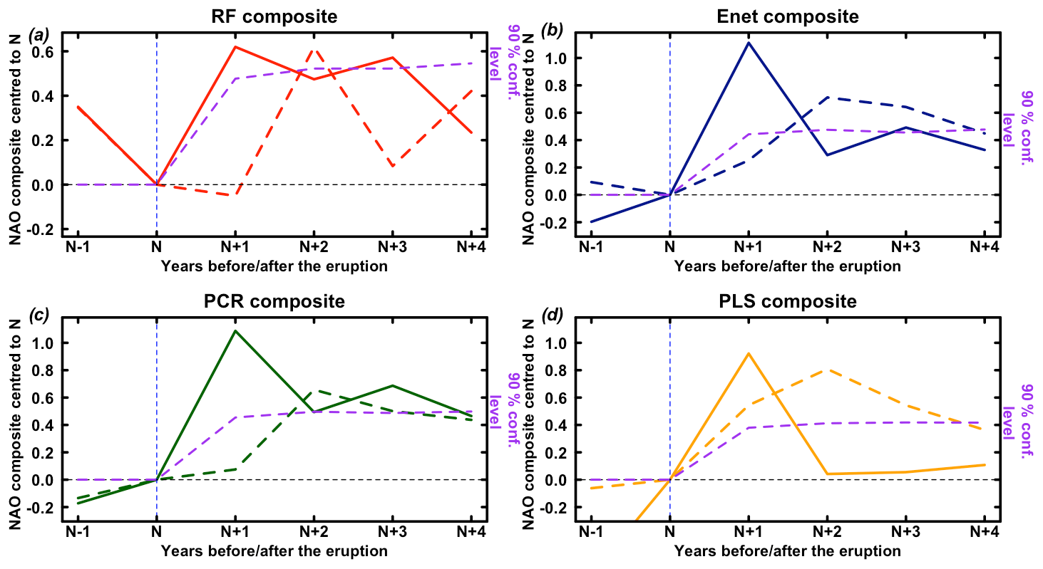
Figure 11 Superposed epoch analysis of the NAO response from 2 years (N−1) before to 5 years after (N+4) the largest volcanic eruptions used by Ortega et al. (2015) (10 eruptions) and the 11 largest from Sigl et al. (2015). All of the composites are centred to their values at the year of the volcanic eruption occurrence. (a) Red line: composite for RF reconstruction response to Sigl et al. (2015) volcanic eruptions. Dashed red line: composite for RF reconstruction response to Ortega et al. (2015) volcanic eruptions. Dashed purple line: Monte Carlo 90 % confidence level (Rao et al., 2019, Sect. S4). (b) Blue line: composite for Enet reconstruction response Sigl et al. (2015) volcanic eruptions. Dashed blue line: composite for Enet reconstruction response to Ortega et al. (2015) volcanic eruptions. Dashed purple line: Monte Carlo 90 % confidence level (Rao et al., 2019, Sect. S4). (c) Green line: composite for PCR reconstruction response Sigl et al. (2015) volcanic eruptions. Dashed green line: composite for PCR reconstruction response to Ortega et al. (2015) volcanic eruptions. Dashed purple line: Monte Carlo 90 % confidence level (Rao et al., 2019, Sect. S4). (d) Orange line: composite for PLS reconstruction response Sigl et al. (2015) volcanic eruptions. Dashed orange line: composite for PLS reconstruction response to Ortega et al. (2015) volcanic eruptions. Dashed purple line: Monte Carlo 90 % confidence level (Rao et al., 2019, Sect. S4).

4 Discussion and conclusion

Discussion, caveats and outlooks

The results presented above regarding the NAO have all been obtained using ClimIndRec. Indeed, they require advanced programming and statistical knowledge to ensure a good estimation of the reliability of the reconstruction performed. This is possible because ClimIndRec offers an integrated package through which parameters and methods can be efficiently tested and compared, together with reliable validation metrics such as the NSCE. Nevertheless, the methodology proposed in ClimIndRec could be further improved in different ways.

ClimIndRec does not deal with missing data in proxy records. This implies selecting exclusively the proxy records that entirely cover the reconstruction period, which thus excludes some existing proxy records. Also, proxy records with gaps are not used in the present version of ClimIndRec as their use in an interpolated version would artificially increase their weight in the reconstruction and thus possibly induce spectral artefacts in the reconstruction (Hanhijarvi et al., 2013). The optimal way to develop a statistical model over the instrumental period is to use as many proxies as possible and as many years of observations as possible. This leads to a paradox since periods that are well covered by observation data are the most recent ones, which are generally less well covered by proxies. However, future versions of ClimIndRec will be dedicated to develop other probabilistic-based reconstruction approaches to deal with missing data such as Bayesian hierarchical models (Tingley and Huybers, 2010a, b, 2013; Tingley, 2012; Cahill et al., 2016) or regularized expectation–maximization algorithms (Schneider, 2001; Mann et al., 2008; Wang et al., 2015). Another point that limits the capacities of ClimIndRec is that it is based on the assumption that teleconnections of the reconstructed mode are stationary in time, while they may depend on the state of the climate system. This is a classical limit for statistical climate reconstructions but it can be evaluated by use of pseudo-proxy methods (e.g. Lehner et al., 2012; Ortega et al., 2015). Regarding this aspect, more complex methods like data assimilation can clearly overcome this weakness by combining model and data. The use of such approaches for the last millennium remains nevertheless very complex primarily because of their computational cost and the lack of data. They are however emerging (e.g. Hakim et al., 2016; Singh et al., 2018). Data assimilation techniques can be very model dependent as highlighted for the ocean over the recent period (Karspeck et al., 2015) so that their reconstruction of a given regional climatic modes can suffer from interference with reconstructions of other aspect of the climate. Thus, dedicated approaches like the ones developed here can be seen as very complementary and may increase our confidence in the reconstructions. Indeed, if different approaches provide very similar results, this can be interpreted as a source of robustness for a given result or reconstruction.

Another caveat concerns the fact that the present version of ClimIndRec does not account for dating uncertainties in proxy records. Future developments of ClimIndRec may allow one to take into account these uncertainties and to provide their estimation along time. For doing so, deeper investigations for each proxy record are needed as these sources of uncertainty are not exhaustively provided in P2k2017. Also, we found that the reconstructions performed by ClimIndRec provide a clear loss of variance over the learning period and the reconstructed period (before 1856; see Table S4). The RF method is the only one that reproduces adequately the NAO amplitude only over the learning period but also provide significant loss of variance over the reconstructed period. This indicates that the loss of variance over the reconstruction period could partly be due to the proxy records themselves and not only to the statistical approach.

A key aspect that has been found within this study is the sensitivity of the results to the validation metric used. Indeed, we also used correlation as the main score for the test period. It appears that this metric was mainly capturing the phasing of the modes in their reconstruction (not shown; Guillot et al., 2015). By using NSCE, we improved the strength of our reconstruction since aspects other than the synchronization were accounted for. This latter metric, which is more classical in prediction evaluation, further highlights that the RF method outperforms most of the others methods, notably the PCR which is a classical method used in paleoclimatology (Cook et al., 2002; Gray et al., 2004; Ortega et al., 2015; Wang et al., 2017). Other metrics of prediction validation exist (e.g. continuous ranked probability score, Gneiting and Raftery, 2007), so a more extensive analysis of the sensitivity of the reconstruction to other metrics for the validation period might be very useful. Thus, the development of other validation metrics in the next versions of ClimIndRec appears an interesting avenue to explore.

5 Conclusions

We have proposed and described here four statistical methods for reconstructing modes of climate variability and have compared them for a particular example: the reconstruction of the NAO. By identifying and minimizing the sources of reconstruction uncertainty due to the method used (Sect. 3.1.1, 3.1.2), the time frame considered (Sect. 3.1.2) and the proxy selection (Sect. 3.1.1), we found the optimal NAO reconstruction. It was obtained for the RF method over the time frame 1000–1972 using the 46 proxy records available for this time frame (Sect. 3.2.1). This method has not been used yet to our knowledge for climate index reconstructions; it clearly outperforms the other methods (Sect. 3.1) and seems thus promising. The reconstruction we obtained is distinguishable from the Ortega et al. (2015) reconstruction but remains significantly correlated with it (r=0.49; p<0.01, over the period 1073–1855).

We have shown that for Enet, PLS and particularly PCR, which is frequently used in paleoclimatology, selecting proxy records with a strong correlation with the index to be reconstructed over the training periods is a good way to improve the NSCE scores, and hence it allows more reliable reconstructions (Sect. 3.1.1). Contrarily, RF gives more reliable reconstructions using the proxy records significantly correlated at the 80 % confidence level with the NAO (Sect. 3.1.1). This may be due to the fact that it has been mainly developed for large datasets (Breiman, 2001). For both cases, gathering new proxy records to the 554 available proxy records collected, may be a reliable source of reconstruction improvement. The inclusion of new NAO-sensitive proxy records in the future may thus lead to better reconstructions. ClimIndRec should allow one to easily perform such new reconstructions.