MOMSO 1.0 – an eddying Southern Ocean model configuration with fairly equilibrated natural carbon

We present a new near-global coupled biogeochemical ocean-circulation model configuration. The configuration features a horizontal discretization with a grid spacing of less than 11 km in the Southern Ocean and gradually coarsens in meridional direction to more than 200 km at 64^∘ N, where the model is bounded by a solid wall. The underlying code framework is the Geophysical Fluid Dynamics Laboratory (GFDL)'s Modular Ocean Model coupled to the Biogeochemistry with Light, Iron, Nutrients and Gases (BLING) ecosystem model of Galbraith et al. (2010). The configuration is unique in that it features both a relatively equilibrated oceanic carbon inventory and an eddying ocean circulation based on a realistic model geometry/bathymetry – a combination that has been precluded by prohibitive computational cost in the past. Results from a simulation with climatological forcing and a sensitivity experiment with increasing winds suggest that the configuration is sufficiently equilibrated to explore Southern Ocean carbon uptake dynamics on decadal timescales. The configuration is dubbed MOMSO, a Modular Ocean Model Southern Ocean configuration.

1 Introduction

The Southern Ocean, also known as the Antarctic Ocean, comprises the southernmost waters of the world oceans. Its southern boundary is set by the Antarctic continent. With regard to its northern boundary to the Atlantic, Pacific and Indian oceans, there is no consensus. One common definition is the location of the Subtropical Front (STF), which separates the relatively saline subtropical waters from the fresher Subantarctic waters. This definition is straightforward because it characterizes the transition from one oceanographic regime to another distinctly different one. However, because the position of the front varies with time, the definition adds complexity to certain analyses such as oceanic inventories. A pragmatic solution is to define a fixed latitude as the northern boundary. We choose 40^∘ S in order to facilitate a comparison with, e.g., Lovenduski et al. (2013) and Dietze et al. (2017).

The atmospheric conditions in the Southern Ocean are characterized by frequent cyclonic storms that travel eastward around the Antarctic continent and high-pressure areas over the poles. This averages to a strong westerly wind belt between 40 and 60^∘ S, and rather weak and irregular polar easterlies from 60^∘ S on southwards. The dominant low-frequency mode of atmospheric variability is summarized by the Southern Annular Mode (Limpasuvan and Hartmann, 1999; Marshall, 2003) which essentially describes the strength and position of the westerly wind belt.

The strong westerly wind belt drives the Antarctic Circumpolar Current (ACC), the “mightiest current in the oceans” (Pickard and Emery, 1990), which is unobstructed by continents. The ACC circumnavigates the globe zonally and thus links the Atlantic, Pacific and Indian oceans. Northward Ekman transport (also driven by the westerlies) drives up- and downwelling (Marshall and Speer, 2012) and is part of a meridional overturning circulation. Among the major processes controlling the net overturning is the so-called “eddy compensation” which largely cancels changes in wind-driven overturning (see Marshall and Radko, 2003; Viebahn and Eden, 2010; Abernathey et al., 2011, 2016; Hallberg and Gnanadesikan, 2006; Thompson et al., 2014; Tamsitt et al., 2017). Further complexity is added by sea ice which modulates air–sea buoyancy fluxes and thus exerts control on convection, a prerequisite for Antarctic Bottom Water (AABW) formation.

Being one of the few places worldwide where deep water (such as AABW) is formed, the Southern Ocean plays a major role in the global carbon budget. Convection events tap into the abyssal ocean and modulate the difference between atmospheric and oceanic CO₂ concentrations which drive net air–sea fluxes. A comprehensive quantitative understanding has not been reached yet, but there is consensus that the variability in the extent to which deep-water masses in the Southern Ocean are isolated from the atmosphere is among the major drivers regulating atmospheric CO₂ variability (e.g., Anderson et al., 2009; van Heuven et al., 2014; Ritter et al., 2017). Consequently, the Southern Ocean has shifted into the limelight of climate research (DeVries et al., 2017; Tamsitt et al., 2017; Langlais et al., 2017, and many more).

To date, the Southern Ocean accounts for almost half of the global oceanic CO₂ uptake from the atmosphere (Takahashi et al., 2012). But there is concern that anticipated climate change (e.g., via changes of atmospheric circulation and sea ice cover) may trigger substantial changes in the Southern Ocean carbon budget (e.g., Heinze et al., 2015; Abernathey et al., 2016) such that the current rate of uptake may well decline in decades to come. Indications for the existence of such potential triggers have been revealed by observation-based atmospheric reanalysis products which show an ongoing strengthening and a poleward shift of the southern westerly winds starting from the 1970s (Thompson and Solomon, 2002).

This observed trend is projected by climate scenarios to intensify (e.g., Simpkins and Karpechko, 2012), and it is straightforward to assume that the associated wind-driven circulation affects biogeochemical dynamics and, eventually, the oceanic carbon budget. A comprehensive understanding of the link between changing winds and oceanic upwelling of carbon-rich deep water (which, in turn, affects surface saturation and net air–sea CO₂ exchange) has, however, not been achieved yet. To this end, the role of mesoscale ocean eddies is especially uncertain: the current generation of coarse-resolution (non-mesoscale-resolving) models suggests that a poleward shift and an intensification of the Southern Ocean westerlies results in a strengthening of the subpolar meridional overturning cell (e.g., Saenko et al., 2005; Hall and Visbeck, 2002; Getzlaff et al., 2016) and, consequently, in increased upwelling of deep water south of the circumpolar flow, which is rich in dissolved inorganic carbon (e.g., Zickfeld et al., 2007; Lenton and Matear, 2007; Lovenduski et al., 2008; Verdy et al., 2007). The net effect here is that changes of the atmospheric circulation reduce the capability of the Southern Ocean to sequester carbon away from the atmosphere. Early on, however, there were indications (e.g., Böning et al., 2008; Hallberg and Gnanadesikan, 2006; Hogg et al., 2008; Screen et al., 2009; Thompson and Solomon, 2002) that this model behavior is a spurious consequence of the underlying eddy parameterization in coarse-resolution models which cannot afford to resolve mesoscale dynamics explicitly. Supporting evidence came from Munday et al. (2014), who showed that mesoscale eddies indeed reduce the sensitivity of oceanic carbon sequestration towards changing wind stress in an idealized model.

To date, we know that very different state-of-the-art approaches to parameterize eddies yield surprisingly similar sensitivities of oceanic carbon inventories to changing winds (Dietze et al., 2017). Further, it has been demonstrated that “the conversion of dense waters back to light waters is sensitive to the degree of parameterization of mesoscale eddies in models” (Spence et al., 2010, 2009). The question, however, as to how a realistic (as opposed to one featuring an idealized geometry) high-resolution coupled biogeochemical ocean-circulation model that actually resolves eddies and carbon dynamics explicitly compares to a coarse-resolution model has not been answered yet. Among the reasons is the prohibitive computational cost that is associated with equilibrating simulated dissolved inorganic carbon concentrations specifically in the deep ocean.

In this model description paper, we present the realistic high-resolution Modular Ocean Model Southern Ocean model configuration (MOMSO 1.0). The configuration features a realistic topography and simulated levels of eddy kinetic energy which do not undercut observed values. The latter suggests that the configuration explicitly resolves a substantial part of mesoscale-related variability rather than relying on parameterizing their effect. MOMSO is designed to explore the sensitivity of the Southern Ocean carbon uptake to atmospheric changes on decadal scales. The configuration is rendered feasible by recent advances in compute hardware and by its similarity to a spun-up coarse-resolution model which delivered the initial conditions for the biogeochemical module. (Note that module refers to the algorithmic entity that calculates the local biogeochemical sources and sinks of the prognostic biogeochemical variables such as nutrients and carbon. The algorithmic entity comprises both the underlying partial differential equations and their approximated representation within the numerical solver.) More specifically, we will showcase that the “level of equilibration” of simulated dissolved inorganic carbon allows us to test the sensitivity of the Southern Ocean carbon budget to anticipated climate change patterns.

In summary, this model description paper aims to (1) describe a new eddying coupled ocean-circulation biogeochemical model configuration of the Southern Ocean and (2) outline research questions for which MOMSO may serve as the base of a tool bench.

The project is dubbed MOMSO, a configuration of the Geophysical Fluid Dynamics Laboratory (GFDL)'s Modular Ocean Model version 4p1 with enhanced resolution in the Southern Ocean. The naming is a homage to the underlying framework, the MOM4p1 release of NOAA's GFDL Modular Ocean Model (Griffies, 2009). The ocean-circulation model is coupled to a sea ice model and the Biogeochemistry with Light, Iron, Nutrients and Gases (BLING) model from Galbraith et al. (2010).

2 Model setup

This model description paper describes simulations with the Modular Ocean Model (MOM), version MOM4p1 coupled to the Sea Ice Simulator (SIS) (Griffies, 2009). The configuration is near global, bounded by Antarctica and 64^∘ N. In the Southern Ocean, the horizontal resolution is higher than 11 km. From 40^∘ S, the meridional grid resolution coarsens towards the north (Fig. 1). There are no open boundaries and there is no tidal forcing.

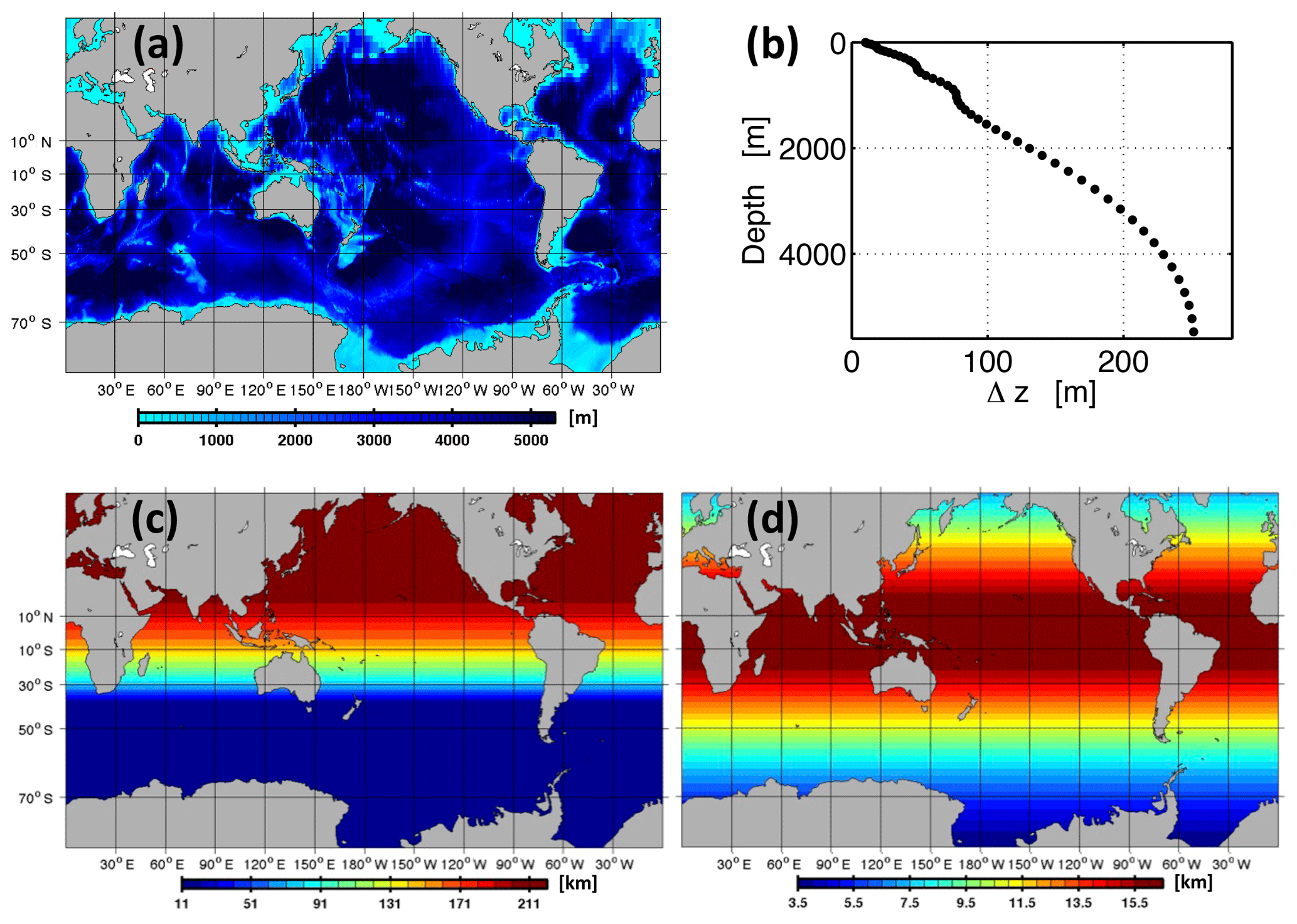
Figure 1 MOMSO model domain and spatial (finite difference) discretization. Panel (a) shows the model bathymetry. Panels (b), (c) and (d) show the vertical, meridional and zonal resolutions, respectively. In total, there are $\mathrm{2400}\times \mathrm{482}\times \mathrm{55}$ grid boxes in zonal, meridional and vertical directions, respectively.

The biogeochemical model BLING (Galbraith et al., 2010) is coupled online to the ocean–sea ice model. Atmospheric CO₂ concentrations are prescribed to a pre-industrial level of 278 ppmv. The respective carbon inventories and fluxes are referred to as “natural carbon”.

2.1 Grid and bathymetry

The underlying bathymetry is ETOPO5 (see Data Announcement 88-MGG-02, Digital relief of the Surface of the Earth. NOAA, National Geophysical Data Center, Boulder, Colorado, 1988). Using a bilinear scheme, the bathymetry is interpolated onto an Arakawa B grid (Arakawa and Lamp, 1977) with 2400×482 tracer grid boxes in the horizontal. The ocean-circulation and sea ice models share the same horizontal grid.

The vertical discretization comprises a total of 55 levels. Figure 1 shows the nominal depth and thickness of each level. The model bathymetry is smoothed with a filter similar to the Shapiro filter (Shapiro, 1970). The filter weights are 0.25, 0.5 and 0.25. The filtering procedure can only decrease the bottom depth; i.e., essentially, it fills rough holes. The filter is applied three times consecutively because we found this to be a good compromise between unnecessary smoothing on the one hand and numerical instabilities introduced by overly steep topography on the other hand in other high-resolution model configurations (Dietze and Kriest, 2012; Dietze et al., 2014). The resulting bathymetry contained lakes which we filled after visual inspection. In addition, we filled narrow inlets which had a width of less than three grid boxes. In total, MOMSO has 42 429 759 wet tracer grid boxes.

Figure 2 Close-up of MOMSO bathymetry in the Drake Passage. The color denotes depths in meters. The red rectangle denotes the area where, from 3250 m down to the bottom, an additional Laplacian horizontal viscosity of 1000 m² s⁻² is applied for stability reasons.

We use the zstar coordinate in the vertical (Stacey et al., 1995; Adcroft and Campin, 2004) which is essentially an extension of the non-linear free-surface method of Campin et al. (2004) to all model levels. The algorithm is well-established for its very accurate conservation of tracers. zstar (z^⋆) is calculated as a function of nominal depth (z), respective water depth (H) and the free sea surface height (η) which varies with time:

$$\begin{array}{}\text{(1)}& z^{\star }=H\left({\displaystyle \frac{z-\mathit{\eta }}{H+\mathit{\eta }}}\right)\end{array}$$

(Eq. 6.6 in Griffies, 2009). The approach overcomes the problem with vanishing surface grid boxes which appears in generic z-level discretization when sea surface height variations are of similar magnitude to the thickness of the uppermost grid box.

2.2 Ocean circulation

MOM4p1 is a z coordinate, free-surface ocean general circulation model which discretizes the ocean's hydrostatic primitive equations on a fixed Eulerian grid. The vertical mixing of momentum and scalars is parameterized by the k-profile parameterization approach of Large et al. (1994) with the same parameters applied in eddy-permitting global configurations of Dietze and Kriest (2012), Dietze and Loeptien (2013), Dietze et al. (2014), and Liu et al. (2010). The relevant parameters are (1) a critical bulk Richardson number of 0.3 and (2) a constant vertical background diffusivity and viscosity of 10⁻⁵ m² s⁻¹. These background values apply also below the surface mixed layer throughout the water column. Both parameterizations of the non-local and the double diffusive (vertical) scalar tracer fluxes are applied.

We apply a state-dependent horizontal Smagorinsky viscosity scheme (Griffies and Hallberg, 2000; Smagorinski, 1963, 1993) to keep friction at the minimal level necessitated by numerical stability. We apply a respective coefficient that sets the scale of the Smagorinsky isotropic viscosity to 0.01. Note that this value is much smaller than the range between 2 and 4 recommended by Griffies and Hallberg (2000) for stability reasons. The rationale behind our choice is to minimize friction which has little physical justification and at the same time has been shown to degrade the performance of ocean-circulation models (e.g., Jochum et al., 2008).

We use the PPM (piecewise parabolic method) advection scheme (Colella and Woodward, 1984) for active tracers because it has been shown to perform well in treating sharp gradients in small-scale circulation (e.g., Carpenter Jr. et al., 1989). For the biogeochemical tracers, we use a flux-limited scheme following Sweby (1984) because we experienced problems in the past with other configurations where negative values occurred for biogeochemical tracers when using non-flux-limited schemes. The choice of two different advection schemes may have repercussions. For example, Lévy et al. (2001) have shown that the choice spuriously affects biogeochemistry in regions of sharp vertical macronutrient gradients such as in oligotrophic regions. We expect that this is not so much an issue in MOMSO because the Southern Ocean vertical nutrient gradients are smoother. Further, we argue that all advection schemes introduce spurious errors (either of diffusive or dispersive nature). These are directly related to the respective property gradient in flow direction. Since all properties (such as temperature, salinity and biogeochemical variables) feature differing gradients, they are affected to a differing degree by the spurious behavior of the advection scheme. Hence, even when using the same advection scheme for all properties, the actual transport of properties is still inconsistent in that they are all affected by differing degrees by spurious errors. This inconsistency can be larger than the inconsistency introduced by switching from one advection scheme to another. Note in this context that we do not apply an explicit horizontal background diffusivity other than the contribution that is implicit to the advection scheme.

Several decades into the spin-up, our configuration became unstable in coarsely resolved places where strong currents met rough topography. This may well have been the result of our very low choice of the Smagorinsky isotropic viscosity (as reviewer 1 suspected). Our fix to the instability problem was to set an additional horizontal isotropic Laplacian viscosity of 600 m² s⁻² from 10^∘ S to 50^∘ N, of 1200 m² s⁻² above 50^∘ N and 1800 m² s⁻² above 60^∘ N outside the Southern Ocean towards the northern boundary of the model domain. This kept the respective oscillations in check. In addition, we added Laplacian viscosity at the exit of the Drake Passage (Fig. 2).

2.3 Sea ice

The ocean component is coupled to a dynamical sea ice module, the GFDL SIS. SIS uses elastic–viscous–plastic rheology adapted from Hunke and Dukowicz (1997). In the standard version, the simulated sea ice impacts sea surface height. This led to a vicious cycle at some places where sea ice attracted ever more sea ice, resulting in unrealistic anomalies in sea surface height and finally in a numerical blow-up of the simulation. Because of the associated computational cost, we did not investigate thoroughly into this but – instead – switched to levitating sea ice by deleting line 1353 in the file ice_model.F90, which reads Ice%p_surf(i,j) = Ice%p_surf(i,j) + grav*x(i,j). Note that this is now also used, e.g., in Hordoir et al. (2019), which is based on the Nucleus for European Modelling of the Ocean (NEMO) framework (Robinson Hordoir, personal communication, 2019).

2.4 Biogeochemistry

In our setup, the ocean–sea ice module is coupled to the BLING ecosystem model of Galbraith et al. (2010). BLING is a prognostic model that, in the basic version, explicitly resolves only four biogeochemical tracers: dissolved inorganic phosphorous, dissolved organic phosphorous, dissolved iron and dissolved oxygen. Here, we use BLING in conjunction with a carbon module that explicitly resolves dissolved inorganic carbon and alkalinity as described, e.g., in Bernadello et al. (2014).

The design idea behind the “reduced-tracer” model BLING is, on the one hand, to minimize the number of prognostic tracers that are actually advected by the ocean-circulation model and, on the other hand, to explicitly resolve the most influential environmental processes that control the net biotic carbon uptake (macro- and micronutrients phosphorous and iron; oxygen which controls heterotrophic respiration). The rationale behind minimizing the number of prognostic tracers is that even simple models (resolving only macronutrients, two phytoplankton species, zooplankton and detritus) are hard to constrain with available observations already (cf. Löptien and Dietze, 2015, 2017, 2019) – a difficulty that increases with the number of tracers. As a favorable side effect, the reduced number of prognostic tracers reduces the computational cost.

2.5 Initial conditions and spin-up procedure

The circulation model starts from rest (i.e., initial velocities are nil) with initial values for temperature and salinity taken from the World Ocean Atlas (WOA) 2009 (Locarnini et al., 2010; Antonov et al., 2009, respectively,). After 20 years of physics-only spin-up, the biogeochemical model is hooked on. In contrast to the physics, we do not use an observational product to initialize the prognostic variables of the biogeochemical model – also because the observations of dissolved iron are so sparse that Orr et al. (2017) suggest not to use them for model initialization. Instead, the initial conditions for the biogeochemical tracers are interpolated from the fully spun-up coarse-resolution configuration used by Dietze et al. (2017) (their “FMCD” simulation). This coarse-resolution configuration is, apart from the spatial discretization (and related parameters in the physical parameterizations of unresolved processes), identical to the MOMSO configuration. A beneficial aspect of this spin-up is that it accelerates the equilibration of the carbon dynamics substantially compared to initializing with an observational products. After a subsequent 60-year spin-up with online biogeochemistry, the model allows already (as we will put forward in Sect. 4) for an investigation of circulation-driven decadal changes of the Southern Ocean carbon budget.

2.6 Boundary conditions and sponges

The boundaries towards the Arctic (i.e., the northern end of the model domain shown in Fig. 1) are closed (i.e., they are represented by solid and flat walls). Temperature and salinity are restored to climatological annual mean estimates (Locarnini et al., 2010; Antonov et al., 2009) in so-called “sponge zones” located in the coarse-resolution domain. The sponge zones along with restoring timescales are shown in Fig. 3. The purpose of these sponges is to ensure realistic deep-water characteristics even though Northern Hemisphere deep-water formation processes are handicapped by the combination of coarse resolution with the absence of eddy parameterizations.

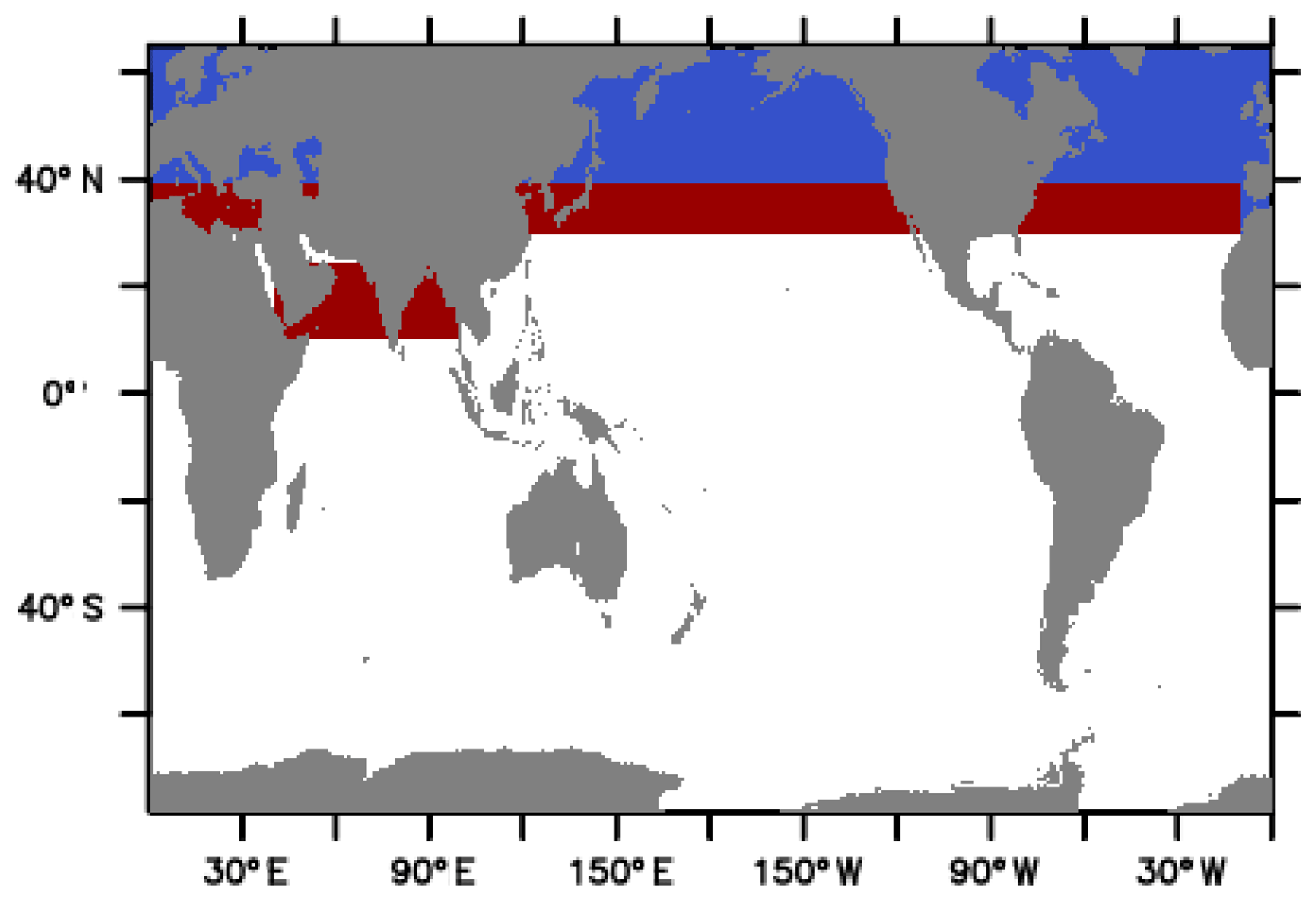
Figure 3 MOMSO domains where temperature and salinity are restored to observed climatological values (Locarnini et al., 2010; Antonov et al., 2009, respectively) throughout the water column. The red and blue patches denote e-folding restoring timescales of 10 and 5 years, respectively.

At the air–sea boundary, we apply climatological atmospheric conditions taken from the Corrected Normal Year Forcing (COREv2; Large and Yeager, 2004). In addition, we apply a surface salinity restoring to climatological values (Antonov et al., 2009) with a timescale of half a year throughout the model domain.

Atmospheric CO₂ concentrations are prescribed to a pre-industrial level of 278 ppmv. Thus, the simulated oceanic carbon is also referred to as “natural carbon”. Biogeochemical air–sea fluxes (of iron) are identical to the ones applied in Galbraith et al. (2010) and Dietze et al. (2017).

This paper refers to output from two simulations dubbed REF and WIND. Both simulations share the same 80-year spin-up described in Sect. 2.5. WIND branches off from REF during the nominal year 1980 and is exposed to ever-increasing wind speeds south of 40^∘ S. The increase is linear at a rate of 14 % in 50 years, consistent with results from a reanalysis of the period 1958 to 2007 (Lovenduski et al., 2013). The rationale behind presenting results from the sensitivity experiment WIND in this model description paper is that they serve as a reference point against which the remaining model drift in REF (which is there since we cannot afford thousands of years of spin-up) can be compared. Based on this comparison, Sect. 4 sketches – very briefly – research questions that may be tackled with MOMSO.

IO-related hardware problems caused data loss such that REF covers the period from 1980 to 2024, while WIND covers 1980 to 2022 only.

Please note that a comprehensive analysis of the sensitivity experiment WIND is beyond the scope of this model description paper. Our major aim here is to show that REF is sufficiently equilibrated so that trends affected by decadal-scale changes in winds can clearly be distinguished against the background trend that is still persistent.

3 Results

In the following, we evaluate our model (simulation REF) by comparing our climatological results from the nominal years 1980–2024 to observational data. One problem is the tradeoff between data coverage and the length of the period the data are representative of. For any given year, the data coverage is insufficient to compile a comprehensive three-dimensional gridded data product. Binning the observational data of several years or even decades into one product closes spatial data gaps, but then this blurs the referencing to an ever-changing (anthropogenically driven) system state. This problem is especially pronounced in the Southern Ocean where in situ data acquisition is complicated by hostile environmental conditions.

The climatological atmospheric boundary conditions which drive our ocean model are representative of the period 1958–2000. Climatological data products are typically biased in that they contain more recent observations, being the result of recent technological advances (such as the development of autonomous platforms). Hence, a model evaluation is not straightforward and it is difficult to define meaningful model–data misfit metrics. Further complexity comes from the fact that misfit metrics must be tailored to the actual application of the model in order to be meaningful.

A potential application for the model configuration presented here is to explore the role of mesoscale features, or eddies, in determining the CO₂ uptake of the Southern Ocean. One hypothesis this model is set up to test is whether spatially unresolved dynamics in IPCC-type coarse-resolution models bias their oceanic carbon uptake sensitivity. In order to come to a meaningful conclusion on this, our high-resolution model has to perform with a fidelity similar or superior to that of IPCC-type coarse-resolution models. In the following, we list and explain our choice of model assessments which we deem relevant in this respect. Wherever applicable, we will follow the approach taken by Sallée et al. (2013a, b), who assessed the performance of CMIP5 models, and Russell et al. (2018), who suggested evaluation metrics for the Southern Ocean in coupled climate models and Earth system models.

Please note that we refrain from using state estimates based on data assimilation such as the Biogeochemical Southern Ocean State Estimate (B-SOSE) (Verdy and Mazloff, 2017) for biogeochemical parameters. On the one hand, these state estimates are especially useful in the Southern Ocean, where observational data are particularly sparse. On the other hand, these estimates rely – especially when observational data are sparse – on the realism of the underlying ocean-circulation biogeochemical model framework. In the case of B-SOSE, the underlying model framework is so similar to our model configuration (high-resolution ocean-circulation model coupled to the biogeochemical model of Galbraith et al., 2010) that we essentially would assess the benefit of the assimilation scheme in fitting observational data rather than assessing our model configuration.

The model–data comparison is divided into the following subsections:

• Ocean circulation (Sect. 3.1), e.g., affects the transport of carbon-rich deepwater to the surface, shapes the locations of fronts and constitutes a major pathway for nutrients that are essential for phytoplankton growth. For the evaluation of surface currents, we use exemplary snapshots showcasing main circulation paths and spatial variability, along with climatological sea surface height which is indicative of the barotropic circulation. More quantitative measures of transport characteristics are provided for the ACC (Drake Passage transport) and the Southern Ocean meridional overturning circulation. Further, we assess the strength of the cyclonic Ross and Weddell polar gyres which are formed by interactions between the ACC and the Antarctic continental shelf. Special emphasis is here on the larger Weddell Gyre. This gyre entrains heat and salt from the ACC and carries them to the Antarctic continental shelves, where deep and bottom waters are produced and thus establish an intermittent connection between the atmosphere (surface ocean) and the deep oceanic carbon (nutrient) pool.

• Eddy kinetic energy (EKE; Sect. 3.2) is an important measure for the mesoscale activity and thus a key proxy for realistically reproduced eddy dynamics. At the surface, the EKE can be derived from the variability of the sea surface height (SSH), a measure that can be directly observed from space by satellite altimetry.

• Surface mixed layer depth (MLD; Sect. 3.3) is determined by (1) the stability of the water column (i.e., the vertical density gradient), (2) wind-induced turbulence which provides energy for eroding the stability and thereby deepens the MLD and (3) air–sea buoyancy fluxes which can, depending on their sign, increase or decrease the stability of the water column and thus shallow or deepen the MLD. The MLD is an important concept or metric because it locates that fraction of the upper water column that is in direct contact with the atmosphere and sets air–sea gradients of temperature and partial pressure of gases (such as carbon dioxide or oxygen). Further, changes in MLD modulate the level of average light levels experienced by phytoplankton: deep MLDs define conditions where phytoplankton spend more time mixed downwards away from the sunlit surface. This reduces phytoplankton growth and associated biotic carbon uptake. Antagonistic to this light deprivation, however, deepening MLDs are typically associated with transports of nutrients (essential for phytoplankton) from depth to the sunlit nutrient-depleted surface.

• Temperatures (Sect. 3.4), which influence the rate of biological turnover, affect the solubility pump of carbon and the density of seawater. Cooling typically results in a reduction of buoyancy and causes convection. Spatial temperature gradients are associated with geostrophic circulation (if they are not salinity compensated). Vertical temperature gradients affect the stability of the water and precondition vertical mixing. The sea surface temperature (SST) can be directly observed from space and therefore is available in an unrivaled (compared to in situ measured properties) spatial and temporal resolution. In contrast, temperature observations at depth are unfortunately much sparser even though deep temperatures determine important processes, e.g., for basal melting, and thus are related to the formation rate of Antarctic Bottom Water (AABW). AABW formation, in turn, affects the solubility and biotic pump of carbon.

• Salinity (Sect. 3.5) is related to the density of seawater. Saltening by brine rejection can cause convection; meltwater, on the other hand, can form buoyant lenses, thus increasing the local stability of the water column which prevents vertical mixing. Spatial salinity gradients are associated with geostrophic circulation (if they are not temperature compensated). Vertical salinity gradients affect the stability of the water column and precondition vertical mixing.

• Sea ice (Sect. 3.6) caps the direct exchange between atmosphere and ocean and thus controls the air–sea gas exchange of CO₂. It also modulates the air–sea buoyancy forcing by, e.g., insulating the surface from heat loss or by brine rejection during ice formation. Further, it shields the surface water from solar irradiance and hampers the assimilation of CO₂ by autotrophic plankton.

• Nutrients (Sect. 3.7) are essential to the growth of autotrophic plankton, and their availability exerts a major control on the biological pump. The most important macronutrient is bioavailable phosphorous (such as phosphate, PO₄), because its availability is essential to all phytoplankton (and cyanobacteria). The distribution of PO₄ is determined by the interplay between the ocean circulation (transporting PO₄ dissolved in seawater) and marine biota which utilize phosphorous to build biomass (typically at the surface) and release PO₄ in the course of degradation of organic material (typically at depth). In addition, we assess simulated iron concentrations since the Southern Ocean is well known for being a site where iron is limiting the growth of autotrophs (e.g., Boyd and Ellwood, 2010). Further, in order to guide the interpretation of simulated PO₄ concentrations at depth, we include a meridional section of dissolved oxygen in this section: oxygen is reset to values close to saturation at the surface, while its sinks in the interior are typically assumed to be linearly linked to interior sources of PO₄ (which is not reset at the surface). Hence, cases where biases in simulated PO₄ concentrations are inconsistent with biases in simulated oxygen concentrations contain information on what exactly is the cause for the simulated biases within the interplay of ocean circulation and biogeochemistry.

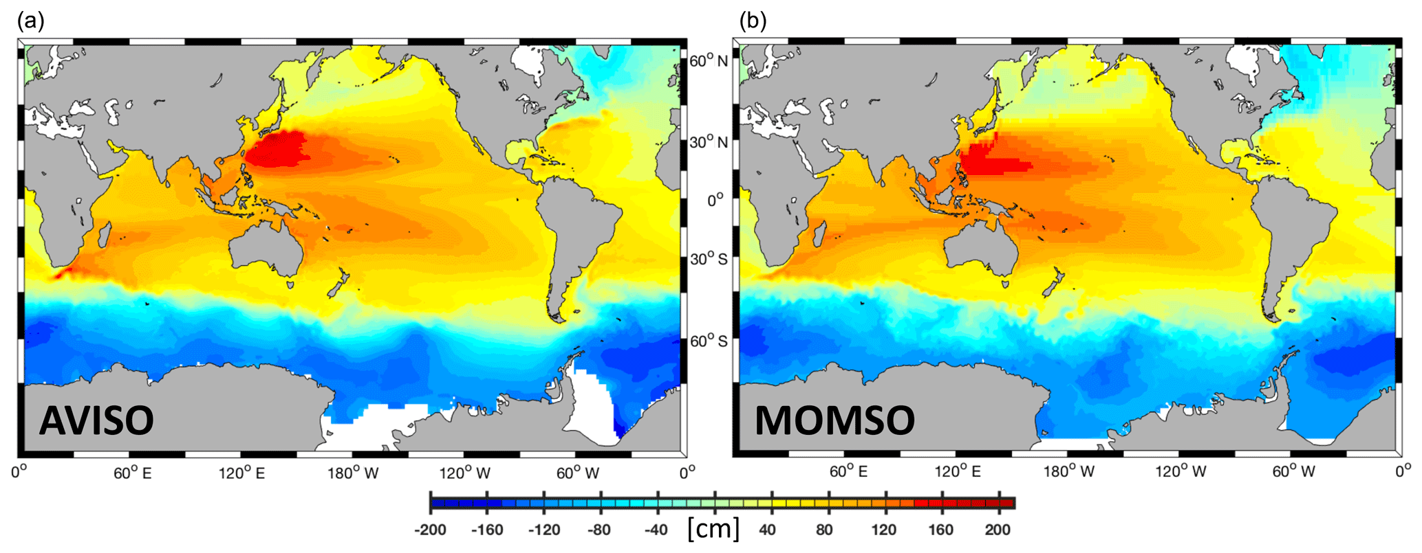
Figure 4 Climatological mean sea surface height in units of centimeters. Panel (a) shows a 1993 to 1998 climatological average observed from space (Maps of Absolute Geostrophic Current (MADT) Aviso data). Panel (b) shows a 6-year average (nominal years 1993 to 1998) simulated with the reference simulation. The white patches in panels (a) and (b) indicate missing data and (spurious) model land mask, respectively.

3.1 Ocean circulation

Figure 4 shows simulated climatological SSH, along with an estimate based on observations from space (Maps of Absolute Geostrophic Current (MADT) Aviso). The model captures the main features of the global barotropic circulation, even in the coarsely resolved domain north of 40^∘ S, such as in the subtropical gyres in both hemispheres north and south of the Equator (positive SSH anomalies) and in the subpolar gyres around 50 and 60^∘ N in the Pacific and Atlantic (negative SSH anomalies), respectively. Further, as indicated by the transition from yellow to blue in the Southern Ocean in Fig. 4, the model reproduces the northern boundary of the Antarctic Circumpolar Current (ACC), also referred to as the northern edge of the Subantarctic Front (SAF).

A quantitative numerical comparison of observed (Aviso) and simulated climatologic surface speeds yields a spatial correlation of 0.6 in the high-resolution domain south of 40^∘ N. The spatial variance in the speed of simulated surface currents is typically 30 % higher than the observational estimate and the respective simulated mean is 20 % higher than in the observations. Apparently, a (yet-to-be-quantified) fraction of this misfit is attributable to errors in the estimates from space (cf. Fratantoni, 2001).

Figure 5 shows exemplary snapshots of the surface velocities as observed from space (Fig. 5a, MADT Aviso) and simulated (Fig. 5b, MOMSO). The boundary conditions of the model are not identical to the atmospheric boundary conditions on that specific day, and the highly non-linear characteristics of eddy dynamics render an “eddy-to-eddy” similarity without data assimilation impossible. So the purpose of Fig. 5 is to demonstrate the similarity of patterns and the major transport pathways in the high-resolution domain south of 40^∘ N. The close-up into the Agulhas retroflection zone (Fig. 6), which is located right in the transition zone from very high to very coarse resolution (see Fig. 1c), highlights that the realism of simulated patterns is sustained right up into the transition to coarser, non-eddy-resolving resolution.

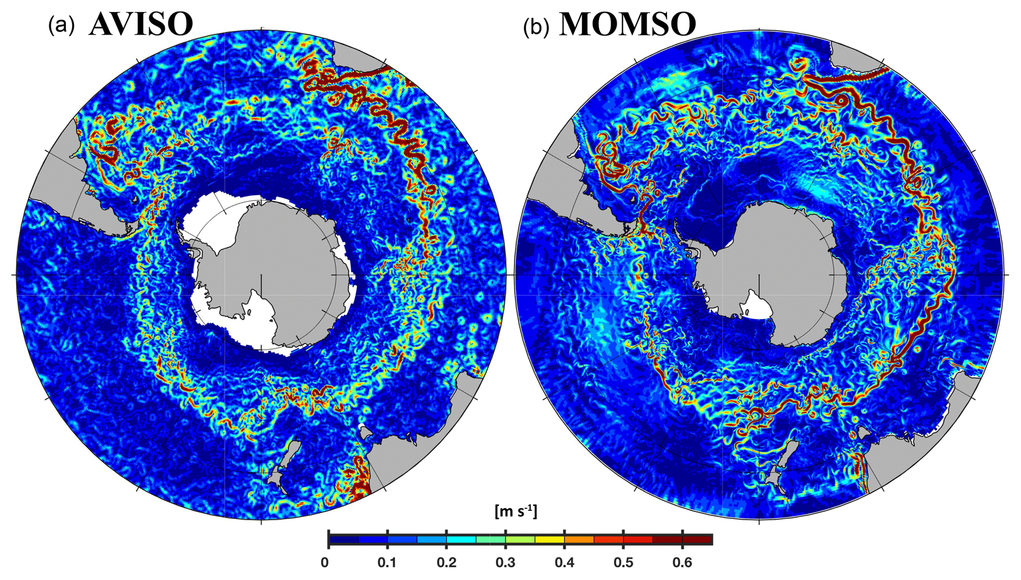
Figure 5 Magnitude of surface velocities. Panels (a) and (b) show typical snapshots as observed from space (Aviso, 3 May 1995) and as simulated (MOMSO, 3 May of nominal year 2020), respectively.

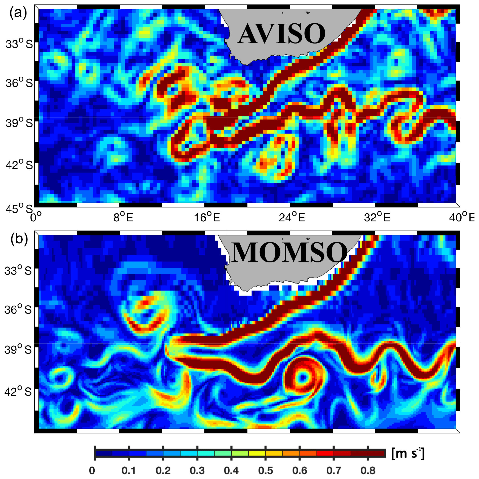
Figure 6 Magnitude of surface velocities. Panels (a) and (b) show typical snapshots as observed from space (Aviso, 3 May 1995) and as simulated (MOMSO, 3 May of nominal year 2020), respectively. This is a close-up from Fig. 5, focusing on those latitudes where the meridional resolution transitions from eddy permitting in the south to eddy prohibiting in the north.

Figure 7 features the simulated transport through the Drake Passage. (Here, we refer to the reference simulation only; simulation WIND is discussed in Sect. 4.) The simulated Drake Passage transport averages to 99 Sv (nominal years 1980–2023). This is biased low compared to available observational estimates that range from 110 to 170 Sv (Withworth, 1983 for 1979; Cunningham et al., 2003 for 1993–2000; Chidichima et al., 2014 for 2007–2011). Note that similar biases have been reported in other high-resolution configurations and may, according to Dufour et al. (2015), be related to a deficient representation of the overflow of dense waters formed along the Antarctic coasts. If so, the ACC bias may well be endemic to z-level models which struggle to represent complex topography (in comparison to more elaborate numerical approaches, e.g., finite elements). A comprehensive investigation is beyond the scope of this paper. But, still, the problem is an intriguing one – especially since, historically, (coarse-resolution) models started out from an opposing bias dubbed “Hidaka's dilemma” (Hidaka and Tsuchiya, 1953), where an excessive ACC transport could only by application of unrealistically high friction be fenced into realistic bounds.

Figure 7 Simulated volume transport of the Antarctic Circumpolar Current through the Drake Passage in units of 10⁶ m³ s⁻¹. The black (red) line refers to the reference (increasing wind) simulation.

In terms of Eulerian meridional overturning in the Southern Ocean, our model values are consistent with the Southern Ocean state estimate of Mazloff et al. (2010): Mazloff et al. (2010) find a surface meridional overturning cell across 32^∘ S of 12±12 Sv and an abyssal cell of 13±6 Sv. We find a climatological mean value for the upper cell of 12±4 and 8±3 Sv for the lower cell. Please note that more elaborate measures such as the physically more meaningful overturning calculated on density coordinates or its approximation given by the residual mean streamfunction (cf. McIntosh and McDougall, 1996; Viebahn and Eden, 2010) are beyond the scope of this paper (which is intended to serve as a model description only).

In terms of transports of the Weddell and Ross gyres, our simulation is slightly biased high. In the Weddell Gyre, we simulate 70 Sv, while published estimates range from 40±8 Sv (Southern Ocean state estimate; Mazloff et al., 2010) to 56±10 Sv (recent SODA estimate Yongliang et al., 2016), 55.9±9.8 and 61–66 Sv (Schröder and Fahrbach, 1999). In the Ross Gyre, we simulate 35 Sv, while published estimates range from 20±5 Sv (Mazloff et al., 2010) to 15–30 Sv (Chu and Fan, 2007) and 37±6 Sv (Yongliang et al., 2016).

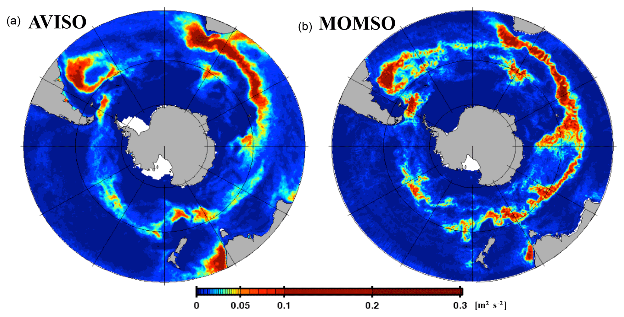
Figure 8 Eddy kinetic energy. Panel (a) is calculated from 1993–1998 satellite altimetry (Maps of Sea Level Anomalies and Geostrophic Velocity Anomalies (MSLA) Aviso data) observations. Panel (b) corresponds to a 6-year average (nominal years 1993 to 1998) calculated from daily averaged surface velocities from the reference simulation. The white patches in the left and right panels indicate missing data and (spurious) model land mask, respectively.

3.2 Eddy kinetic energy and sea surface height

Figure 8 shows that the simulated climatological EKE reproduces the amplitudes and spatial pattern observed from space (Maps of Sea Level Anomalies and Geostrophic Velocity Anomalies (MSLA) Aviso data) as can be expected from high-resolution configurations (e.g., Delworth et al., 2012; Barnier et al., 2006). This applies especially in the high-resolution region south of 40^∘ S, where typical deviations in simulated EKE are rather small (<0.03 m² s⁻²) compared to the maximum values found in the ACC (>0.3 m² s⁻²; cf. Fig. 9). The correlation coefficient between simulated and observed EKE patterns is 0.7. The simulated EKE features 7 % more spatial variance and an average of 8 % more energy within the high-resolution domain south of 40^∘ S. By averaging all simulated values with their immediate spatial neighbors two times consecutively, the simulated variance levels become more similar to observed values and the respective correlation increases to 0.71. We interpret this as an indication that the model resolution is higher than the effective spatial resolution of the MSLA Aviso data. This may also explain why simulated EKE amplitudes are generally higher than estimates from space (cf. Fratantoni, 2001).

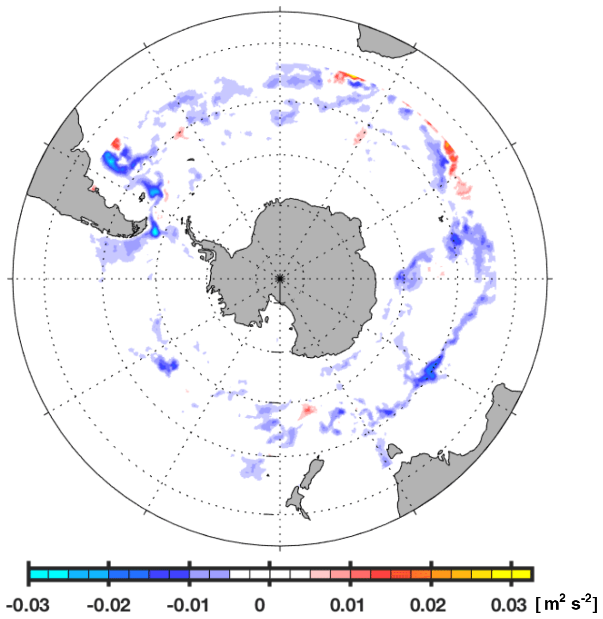
Figure 9 Difference between observed and simulated eddy kinetic energy. Blue colors denote regions where the observed levels calculated from 1993–1998 satellite altimetry (MSLA Aviso data) observations are lower than simulated levels. The region outside the high-resolution nest (north of 40^∘ S) is masked by a white patch.

We conclude that we found no evidence of an underestimation of simulated mesoscale activity. This, in turn, implies that our combination of spatial resolution and (parameterization of) friction in the Southern Ocean is suitable to allow for investigations into eddy-driven processes.

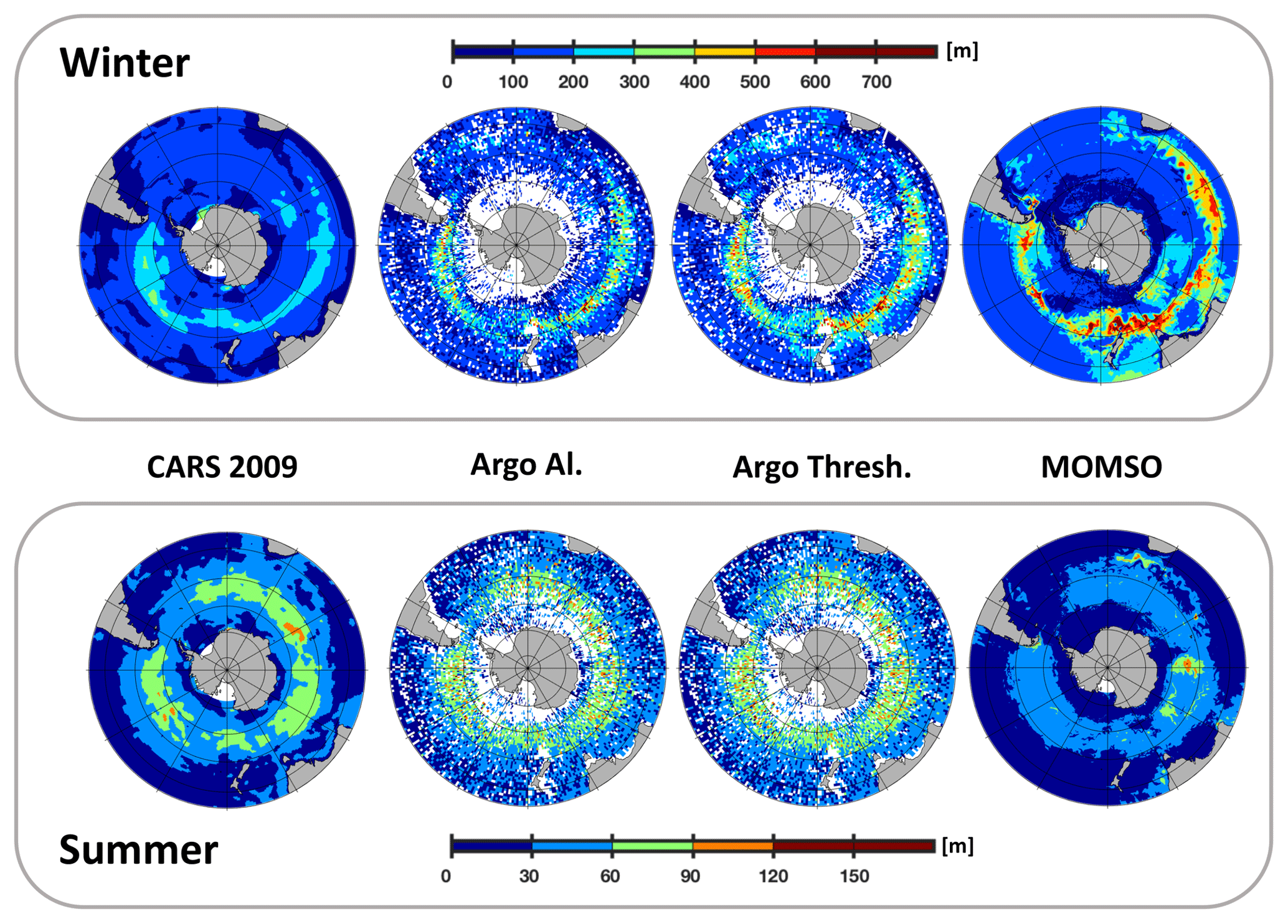
Figure 10 Surface mixed layer depth in units of meters. The upper (lower) line refers to austral winter (summer). The columns refer to (observed) CARS 2009 climatology based on Condie and Dunn (2006), Argo Al. and Argo Thresh. computed from (observed) profiles of Argo floats using two different methods by Holte et al. (2017) and our simulation (MOMSO). White patches in Argo Al. and Argo Thresh. denote missing data.

3.3 Surface mixed layer depth

MLD is a concept that locates that fraction of the upper water column that is well mixed. MLD is typically derived from vertical profiles of temperature and salinity rather than from direct measurements of mixing intensity (i.e., turbulence). As a consequence, algorithms calculating MLDs struggle with distinguishing between identifying actively mixed layers and those which have been actively mixed in the past but are no longer fed by energy fueling actual turbulence and associated mixing. The first three columns of Fig. 10 provide a comparison between contemporary (in the sense that they are still used in current peer-reviewed literature) databases and algorithms to compute MLD: CARS 2009 distributed by CSIRO http://www.marine.csiro.au/~dunn/cars2009/ (last access: 1 November 2019) and introduced by Condie and Dunn (2006) is predominantly based on historical conductivity–temperature–depth (CTD) observations, while both Argo Al. and Argo Thresh. are based on observations from Argo floats. The difference between Argo Al. and Argo Thresh. is the algorithm used to derive MLDs in Holte et al. (2017). We find a high correlation between the different algorithms Argo Al. and Argo Thresh. in the region south of 40^∘ S (0.98 and 0.91 in summer and winter, respectively). The correlation from one database to another (i.e., Argo vs. CARS 2009) is much lower (≈0.7 for both winter and summer – irrespective of algorithm). Argo Thresh. is closest to our simulated pattern (fourth row in Fig. 10), and we find correlations of 0.5 and 0.6 in summer and winter, respectively.

In summary (cf. winter statistics in Fig. 11), we find that the average of variance in simulated MLDs is higher than in the observations and that the differences in correlation from one MLD product to another are comparable to our model–observation misfit. In terms of bias, we find that our simulated winter MLD is, on average, 18 m deeper than Argo Thresh. This is a major improvement compared to (coarse-resolution and fully coupled) CMIP5 models which feature similar correlations but winter mixed layer depths biased low by typically 50–100 m (Sallée et al., 2013a, their Fig. 4a).

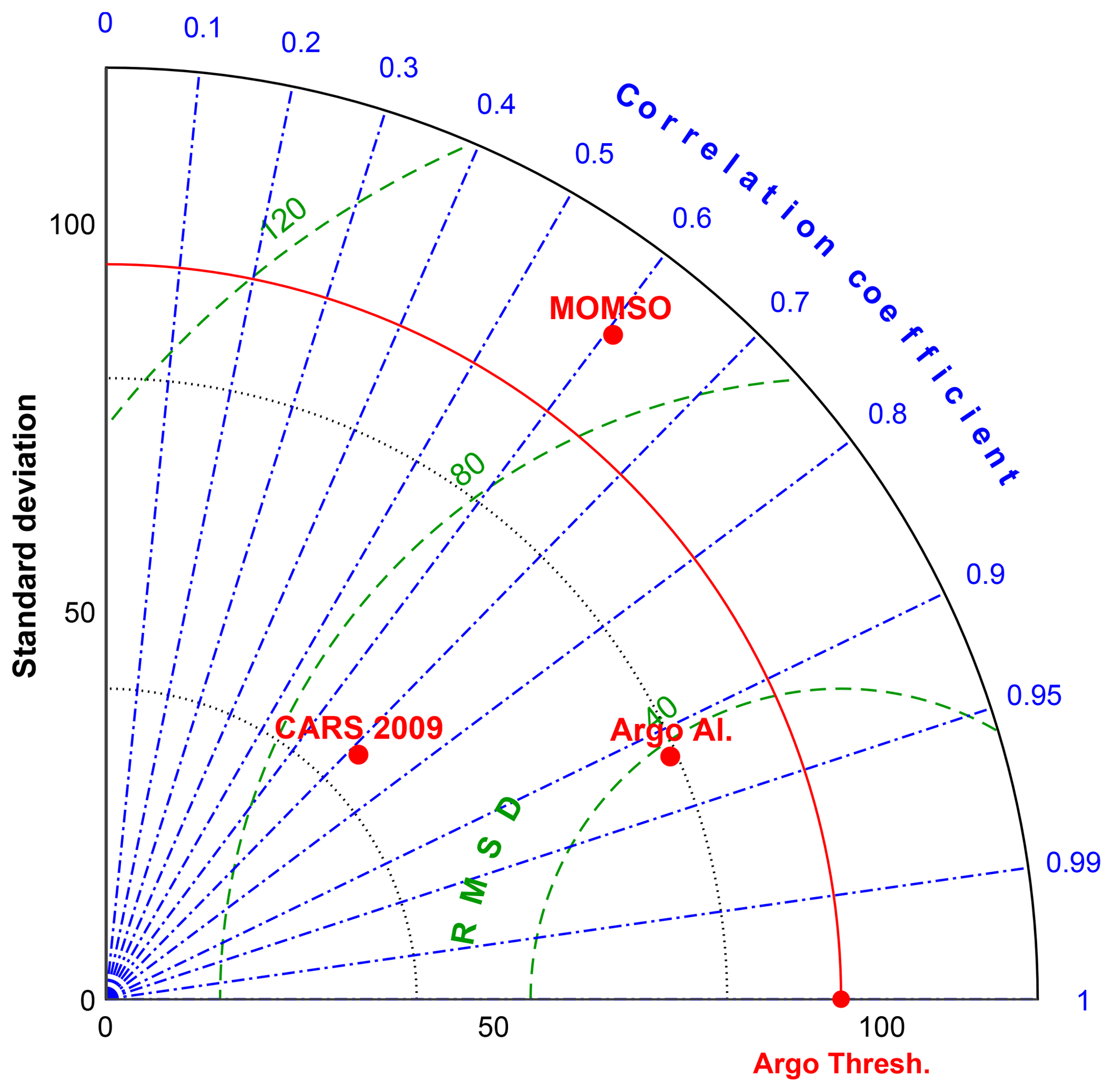
Figure 11 Taylor diagram of surface mixed layer depth in austral winter referred to as Argo Thresh. observational data compiled by Holte et al. (2017). The units for the standard deviation and root mean square deviations are meters. Argo Al. refers also to observational data compiled by Holte et al. (2017) but based on a different algorithm. CARS 2009 is a climatology based on observations compiled by Condie and Dunn (2006), and MOMSO refers to the high-resolution reference simulation presented in this study.

3.4 Temperature

Figure 12 shows a comparison of the simulated SST with WOA09 (Locarnini et al., 2010) and Argo-float-based (Roemmich and Gilson, 2009) observations. The overall pattern is well reproduced – an exception being a local high bias of about 3 ^∘C close to the Antarctic coast (between 120 and 160^∘ E). Averaged over the Southern Ocean (Fig. 13), the simulated SSTs are within the observational range (although at the lower edge) of the years 1960 to 2010 (Fig. 14 calculated from HadISST; Rayner et al., 2003).

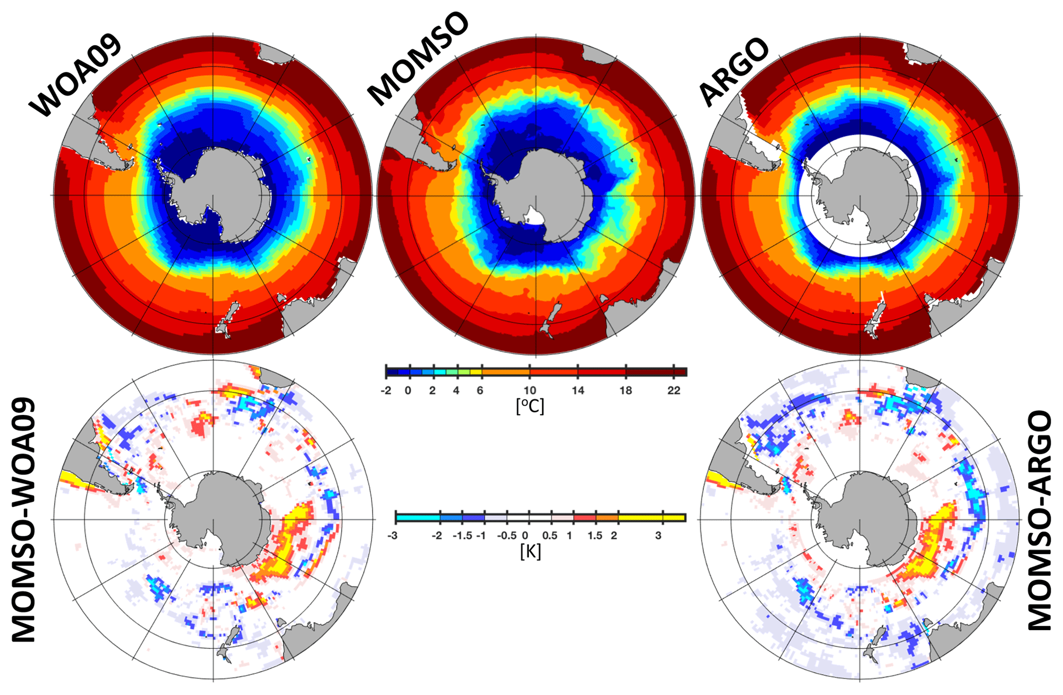
Figure 12 Climatological mean sea surface temperature. WOA09 and Argo (2004–2017 period) refer to observations compiled by Locarnini et al. (2010) and Roemmich and Gilson (2009), respectively. MOMSO refers to an average over the nominal 1993–1998 period of the reference simulation. The upper (lower) panels show sea surface temperature (differences).

Figure 15 summarizes the fidelity of simulated temperatures in the interior. Following Sallée et al. (2013b) and their density-based water mass criteria, we discuss the five major water masses (subtropical water, mode water, intermediate water, circumpolar deep water, bottom water) separately:

• With subtropical water (TW), MOMSO features a slight cold bias at the surface (less than 0.5 ^∘C) and a warm bias of ≈1 ^∘C in the interior (Fig. 15). This is apparently very good when compared against the 2.7^∘ warm bias in the CMIP5 models (Sallée et al., 2013b). There are, however, indications that the 2.7^∘ bias is a consequence of biased air–sea heat fluxes in the Southern Hemisphere in the coupled models rather than the consequence of an unrealistic oceanic circulation.

• The subduction of surface waters is dominated by mode water (MW) in the Southern Ocean. Hence, MW is an important agent in sequestering anthropogenic carbon away from the atmosphere. MOMSO's MW is too warm by ≈1 ^∘C, which compares favorably to the much larger bias of an ensemble mean bias of 3.5 ^∘C in CMIP5 models (Sallée et al., 2013b).

• Intermediate water (IW) is a denser type of MW which ventilates the thermocline and is sequestered away from the atmosphere longer than MW because it protrudes deeper into the water column. MOMSO's IW is biased warm by ≈1.1 ^∘C (Fig. 15), which compares favorably against the 3.5 ^∘C warm bias in CMIP5 models (Sallée et al., 2013b).

• During its formation at the surface, circumpolar deep water (CDW) taps into the abyssal waters rich in natural carbon. Hence, it plays a key role for the oceanic sequestration of natural carbon dioxide (e.g., Le Quéré et al., 2009). MOMSO overestimates the CDW temperature by ≈1 ^∘C. This is substantially more than the 0.4 ^∘C overestimation of the CMIP5 ensemble mean but still within the envelope of the ensemble, which peaks at an overestimation of 1.5 ^∘C (Sallée et al., 2013b).

• MOMSO overestimates Antarctic Bottom Water (BW) temperatures by 1 ^∘C, while the CMIP5 ensemble mean compares more favorably with an underestimation of only 0.4 ^∘C. These biases are consistent with MOMSO featuring too much sea ice coverage which caps the ocean from the cooling atmosphere (cf. Sect. 3.6). Likewise, CMIP5 models tend to underestimate sea ice coverage (Turner et al., 2013), which may overly expose the ocean to the cooling atmosphere and thereby cause the respective cold bias in BW temperature.

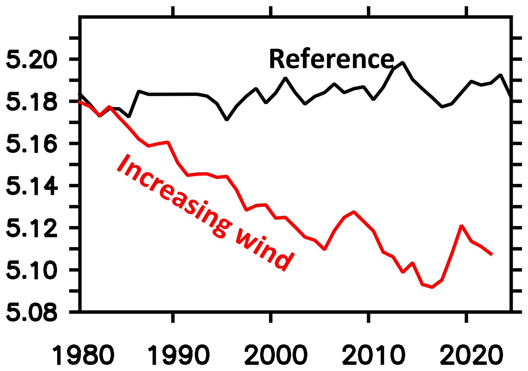
Figure 13 Simulated sea surface temperature averaged over the Southern Ocean (i.e., south of 40^∘ S). The black (red) line refers to the reference (increasing wind) simulation.

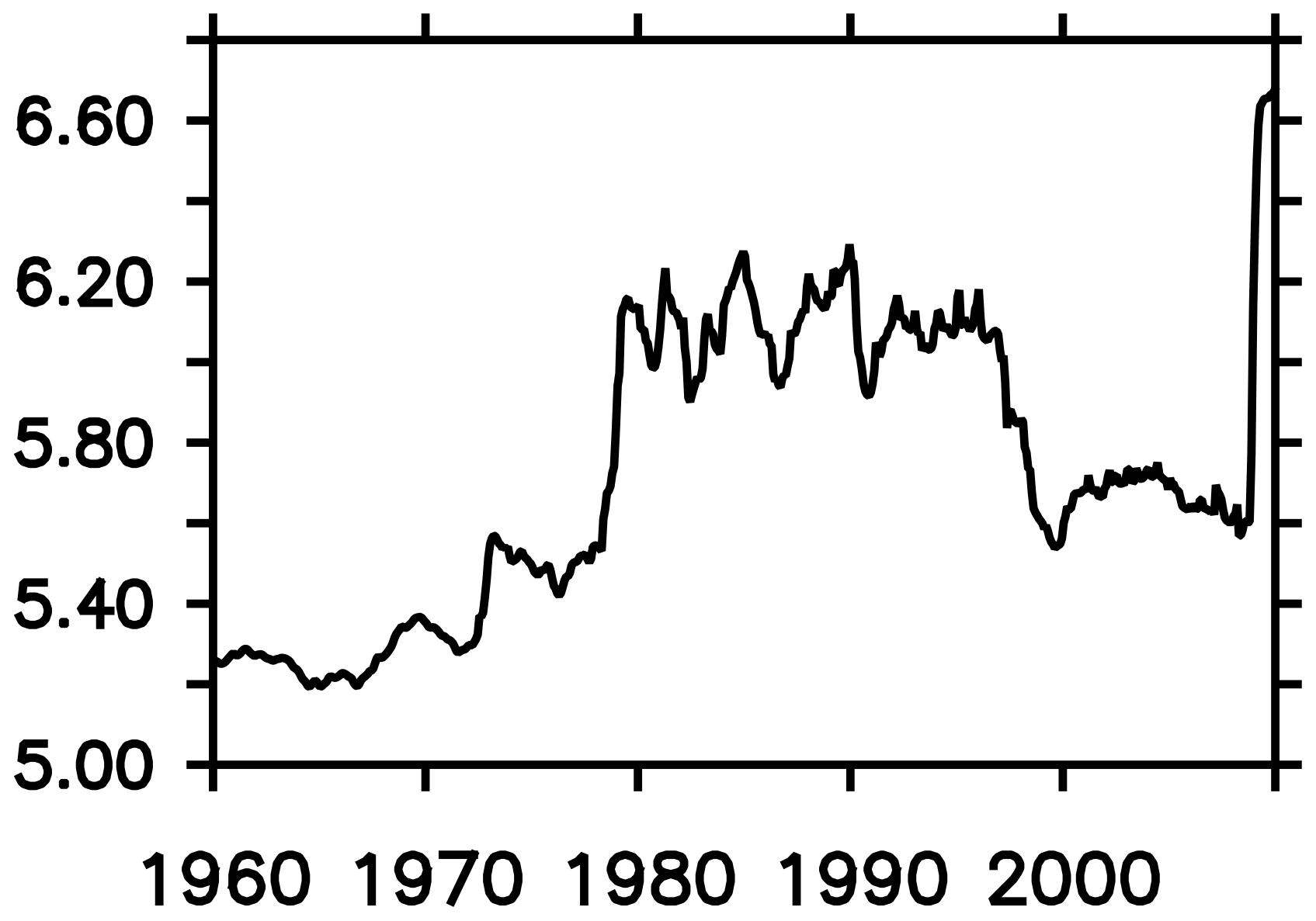
Figure 14 Observational estimate of annual mean sea surface temperatures south of 40^∘ S calculated from HadISST (Rayner et al., 2003).

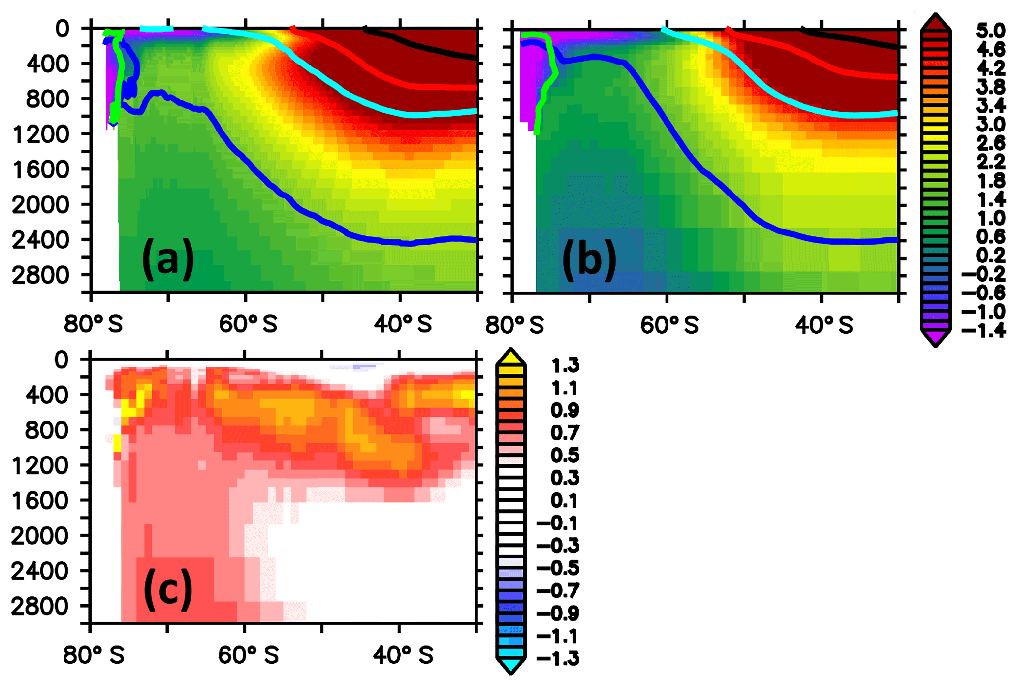
Figure 15 Zonally averaged meridional section of temperature in units of ^∘C. Panel (a) refers to simulated concentrations averaged over the nominal 1993–1998 period of the reference simulation; (b) refers to observed climatological values (WOA09); (c) refers to the difference between simulated and observed values, with blue colors denoting simulated temperatures that are biased low. The thick black, red, cyan, blue and green contours refer to mean densities (Sallée et al., 2013b, their Table 2) of subtropical water, mode water, intermediate water, circumpolar deep water and bottom water, respectively.

3.5 Salinity

Figure 16 shows a comparison of the simulated climatological mean sea surface salinity (SSS) with three observation-based products (WOA09, Antonov et al., 2009; Argo, Roemmich and Gilson, 2009; and SMOS, Köhler et al., 2015). Within the spatially highly resolved Southern Ocean, the simulated sea surface salinity is in good agreement with the observations. Towards the north, where the resolution coarsens, the model fidelity disintegrates; particularly in the Atlantic and Indian sectors, the model is biased low.

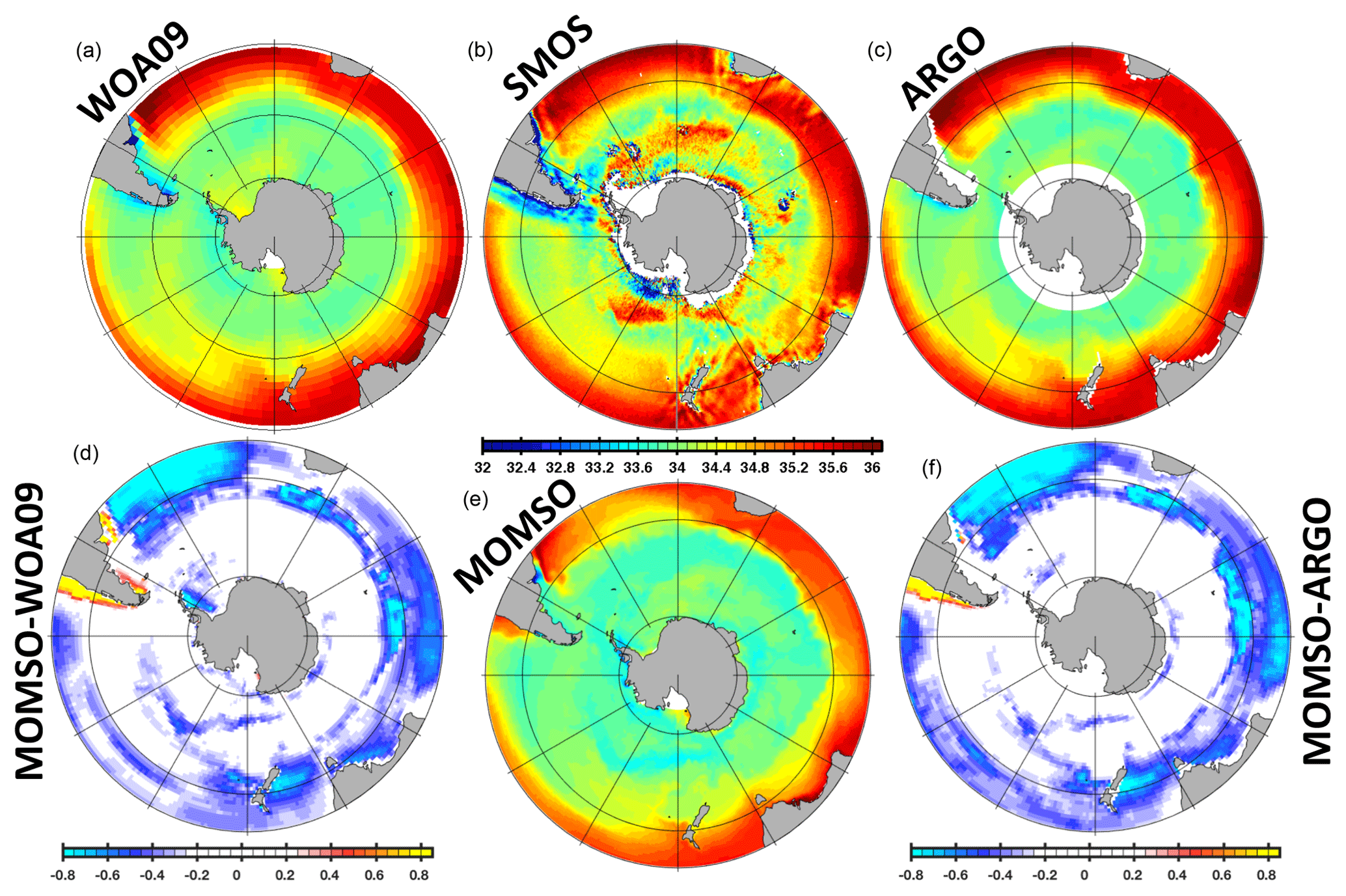
Figure 16 Climatological mean sea surface salinity in psu. WOA09, Argo (2004–2017 period) and SMOS in the upper panels refer to observations compiled by Antonov et al. (2009), Roemmich and Gilson (2009) and Köhler et al. (2015), respectively. MOMSO in the lower panel refers to an average over the nominal 1993–1998 period of the reference simulation. MOMSO-WOA09 and MOMSO-Argo refer to sea surface salinity differences between the reference simulation and respective observations.

Averaged over the Southern Ocean, the simulated SSS is biased low (compare reference in Fig. 17) compared to recent observational estimates during 2005–2017 (Fig. 18). Figure 17 suggests that increasing winds can increase simulated SSSs up to observed values. This could be interpreted as a mismatch between the climatological forcing (representing the years 1958–2000) and the observation period. (Please note that a comprehensive analysis is beyond the scope of this model description paper.) Figure 17 suggests further that the surface salinity restoration (cf. Sect. 2.6) is weak enough to allow for substantial SSS dynamics in response to, e.g., increasing winds.

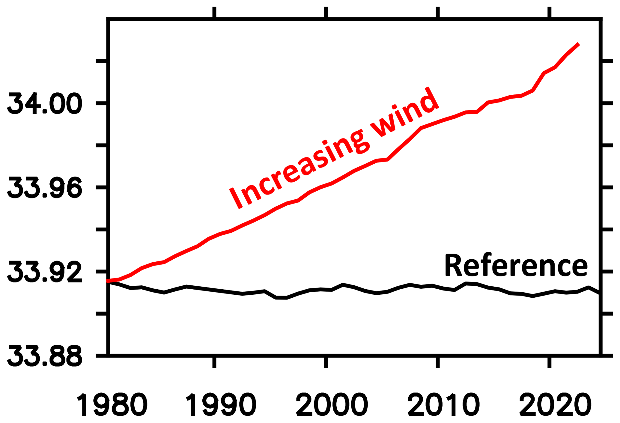
Figure 17 Simulated sea surface salinity averaged over the Southern Ocean (i.e., south of 40^∘ S) for the nominal years 1980–2024. The black (red) line refers to the reference (increasing wind) simulation.

Figure 19 summarizes the fidelity of simulated salinities in the interior. Following Sallée et al. (2013b) and their density-based water mass criteria, we discuss the five major water masses (subtropical water, mode water, intermediate water, circumpolar deep water, bottom water) separately:

• For TW, MOMSO is biased low by 0.5 at the surface, and this makes the simulated TW too light in comparison with WOA09 observations. Sallée et al. (2013b) find a smaller ensemble mean bias of 0.2 in the CMIP5 models which is – in contrast to MOMSO – enhanced, in terms of biasing the density towards smaller values, by a 2.7 ^∘C warm bias.

• For MW, MOMSO is biased low by 0.1 at the surface and high by 0.1 in the interior. This is in line with the overall poor performance of CMIP5 models in representing the MW (Sallée et al., 2013b). Coincidentally, the ensemble mean over all the CMIP5 models averages to a very small fresh bias of 0.02.

• For IW, MOMSO is, again, biased low by 0.1 at the surface and high by 0.1 in the interior. This dampens the equatorward protruding of IW's salinity-minimum signature. Compared against the high bias of only 0.008 in the ensemble mean over all the CMIP5 models, MOMSO's bias appears substantial. Compared, however, against individual CMIP5 models whose characteristics vary widely (Sallée et al., 2013b), MOMSO is comparable (i.e., within the envelope spanned by the CMIP5 models).

• For CDW, MOMSO is biased high by 0.07 south of 75 ^∘S at the surface and less than 0.02 equatorwards. These small biases are well within the range set by the CMIP5 models and of the same order of magnitude as the bias of 0.02 of the CMIP5 ensemble.

• For BW, MOMSO's bias is identical to the high bias of 0.06 in the CMIP5 ensemble mean (Sallée et al., 2013b) and much better than the up-to-0.5 biases of many individual CMIP5 members. The bias is consistent with the bias in sea ice: an overestimated ice production releases too much brine and shields the ocean from atmospheric cooling. This drives spuriously elevated salinities and temperatures.

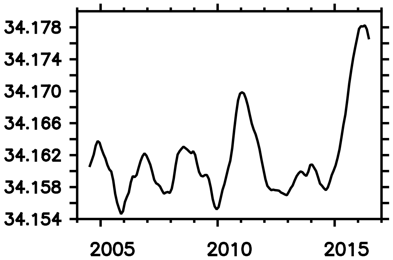
Figure 18 Observed sea surface salinity averaged over the Southern Ocean (i.e., south of 40^∘ S) based on Argo data (Roemmich and Gilson, 2009).

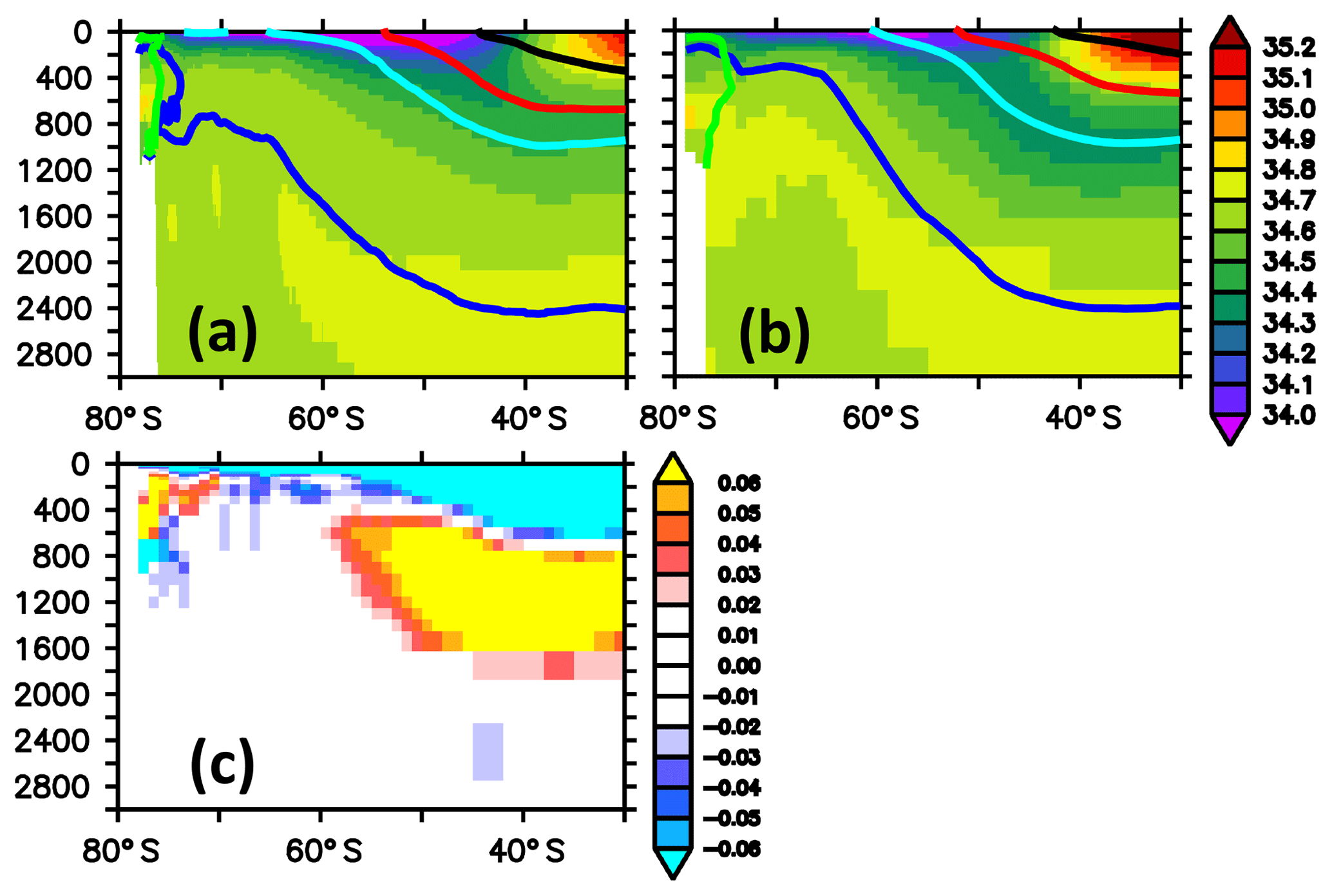
Figure 19 Zonally averaged meridional section of salinity. Panel (a) refers to simulated salinities averaged over the nominal 1993–1998 period of the reference simulation. Panel (b) refers to observed climatological salinities (WOA09). Panel (c) refers to the difference between simulated and observed values, with blue colors denoting simulated salinities that are biased low. The thick black, red, cyan, blue and green contours refer to mean densities (Sallée et al., 2013b, their Table 2) of subtropical water, mode water, intermediate water, circumpolar deep water and bottom water, respectively.

3.6 Sea ice

Figure 20 shows a comparison of the simulated number of sea-ice-covered months per year with an observation estimate (HadISST; Rayner et al., 2003). Overall, the agreement is good, with the following two exceptions: (1) in the Weddell and Ross seas, the period of ice coverage is underestimated by 2 months. We speculate that this triggers elevated air–sea momentum fluxes and, eventually, biases the respective gyre strengths high (cf. Sect. 3.1). (2) Overall, the simulated ice extent is biased high (compare Fig. 21, black line, to Fig. 22). Following Russell et al. (2018) we compare the data, in addition, against the fractional sea ice coverage obtained from the National Snow and Ice Data Center (NSIDC; ftp://sidads.colorado.edu/ pub/DATASETS/NOAA/G02202_v2/, last access: 1 September 2019). The comparison in Fig. 23 confirms the impression that the model overestimates sea ice coverage. Figure 21 suggests that increasing the wind speeds to levels that are more representative of the time period of observations shown in Fig. 22 alleviates this model bias. In addition, Fig. 23 reveals that the model bias features a seasonality with underestimation in January until March and an overestimation of ice coverage from May to December. Ranked against the current generation of IPCC models, MOMSO fits well into the envelope of the ensemble reported by Turner et al. (2013).

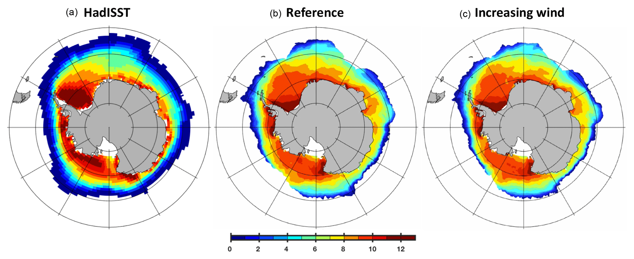
Figure 20 Ice-covered months in a year. Panel (a) refers to a 1980–2000 average based on the HadISST observational estimate (Rayner et al., 2003). Panels (b) and (c) refer to the nominal year 2022 of the reference and increasing wind simulations, respectively.

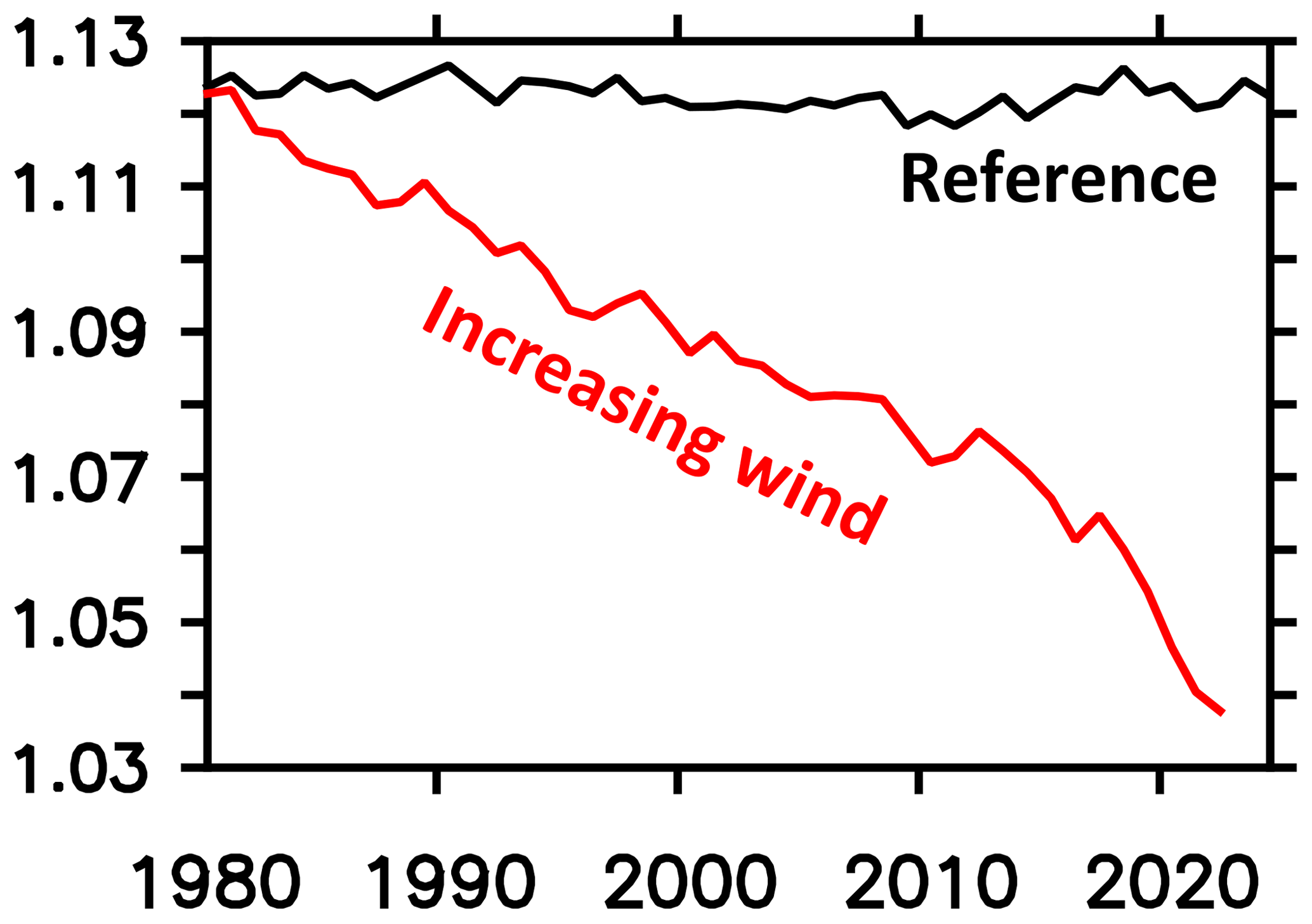
Figure 21 Simulated annual mean sea ice cover south of 40^∘ S in units of 10⁷ km². The black (red) line refers to the reference (increasing wind) simulation.

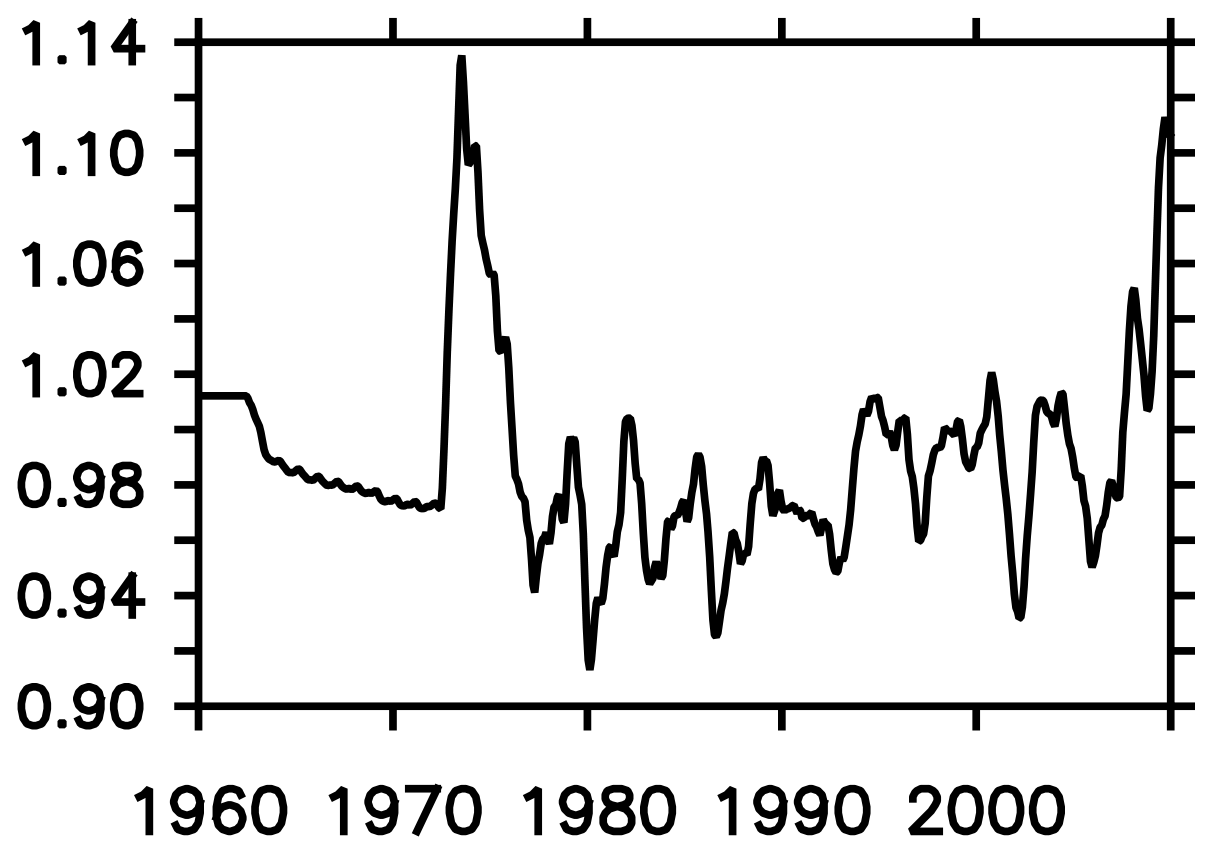
Figure 22 Observational estimate of annual mean sea ice cover south of 40^∘ S in units of 10⁷ km² calculated from HadISST (Rayner et al., 2003).

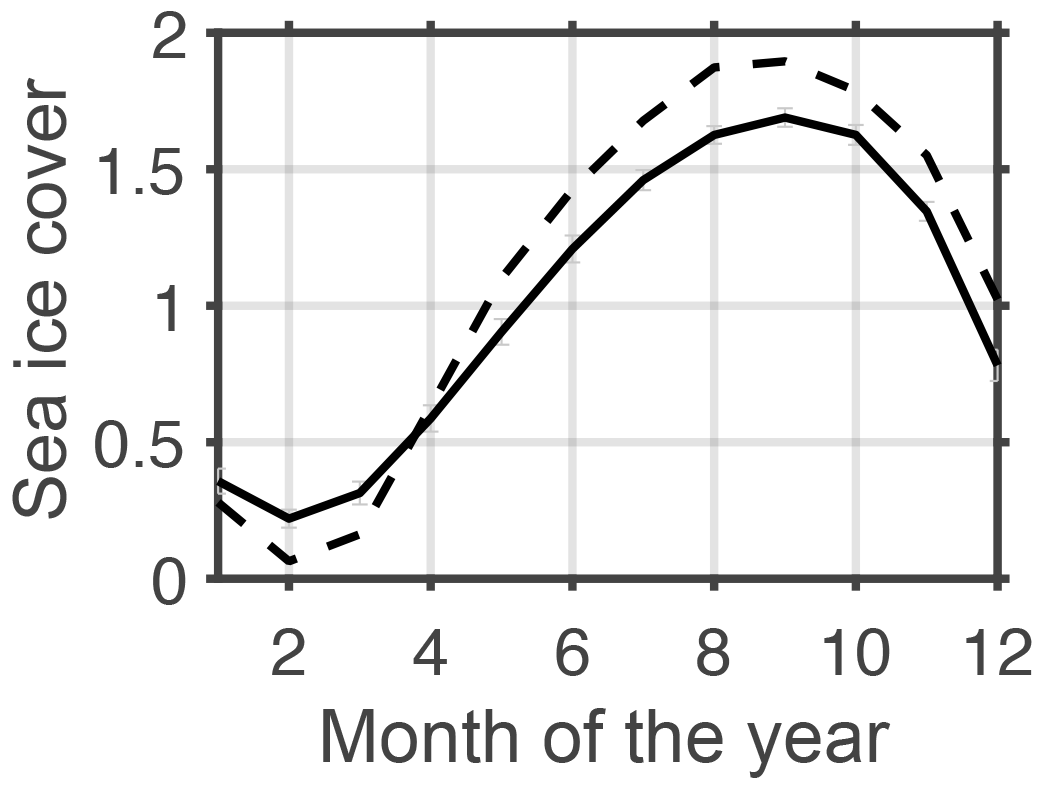
Figure 23 Simulated (dashed line, reference simulation) and observed (solid line, reanalysis from NSIDC) climatological annual cycle of sea ice cover south of 40^∘ S in units of 10⁷ km².

3.7 Nutrients

Simulated Southern Ocean PO₄ surface concentrations are biased low, locally down to 0.6 mmol P m⁻³ (Fig. 24a, c). The reason is not straightforward to identify because it could be associated with a deficient physical module, a deficient biogeochemical module or both. In the following, we will present an indication that the problem is associated with a deficient formulation of iron limitation, argue why the formulation of light limitation is unlikely to be the main problem and put the model–data misfit into perspective.

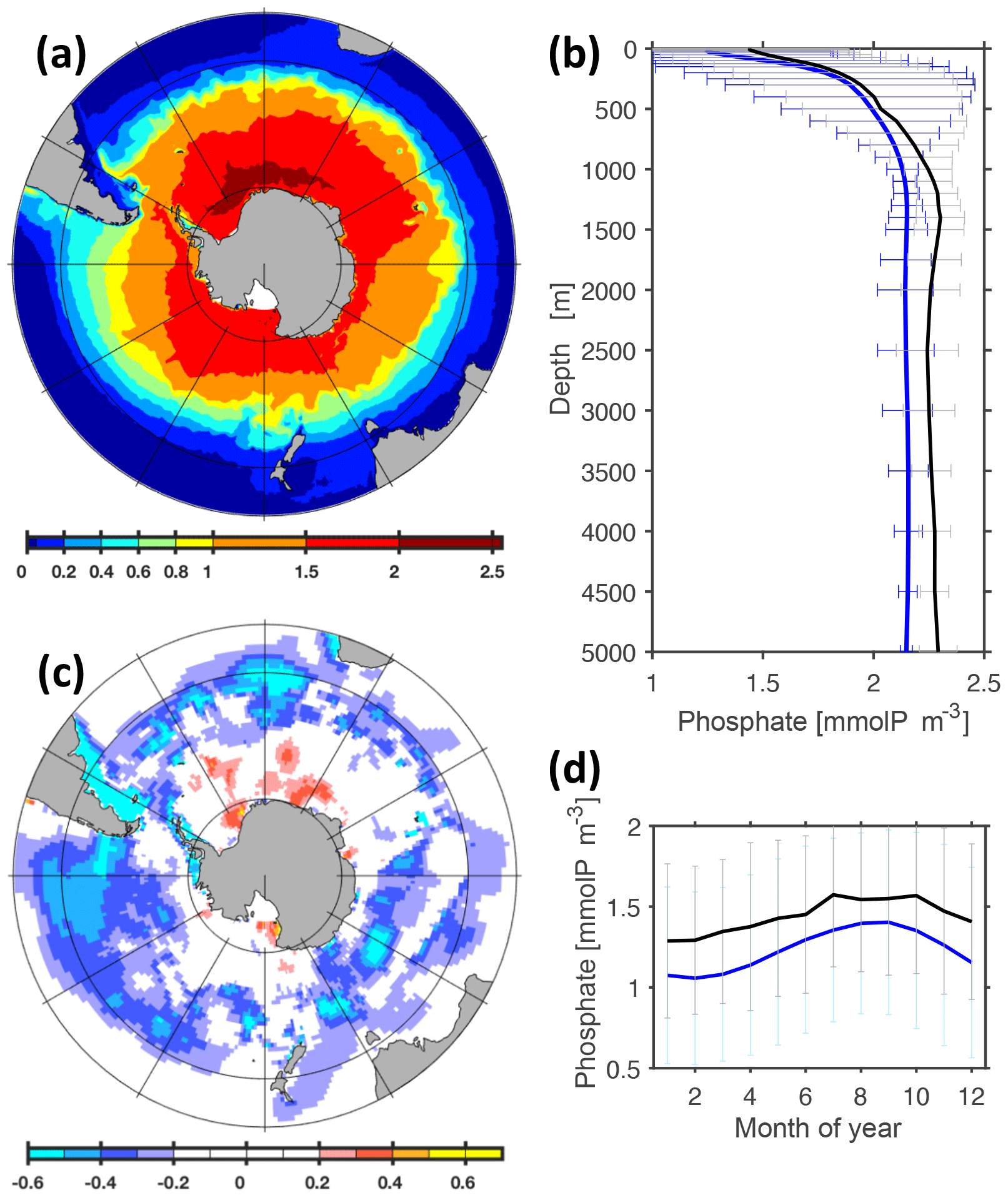
Figure 24 Comparison of simulated and observed phosphate concentrations. Panel (a) refers to simulated surface phosphate concentrations (reference simulation, averaged over nominal years 1993 to 1998). The color bar denotes phosphate concentrations in units of mmol P m⁻³. Panel (b) shows simulated (blue line) and observed (black line) phosphate concentrations averaged horizontally in the Southern Ocean (i.e., south of 40^∘ S), along with their respective spatial standard deviations (grey and blue horizontal bars). Panel (c) shows the difference between simulated and observed (Garcia et al., 2010) surface concentrations. Panel (d) shows the simulated (blue line) and observed (black line) seasonal cycle of dissolved phosphate concentration at the surface calculated as monthly means averaged over the Southern Ocean.

Southern Ocean uptake of PO₄ in the sunlit surface by autotrophic phytoplankton is known to be limited by the availability of light and the availability of the micronutrient iron. Figure 25 features a comparison of simulated iron concentrations with observations. Even though the spatial and temporal coverage of iron measurements is still sparse, the emerging pattern is one where the simulated biotic iron drawdown at the surface appears to be too strong. Surface iron concentrations are biased low, just like the PO₄ concentrations, and they appear so throughout an annual cycle. Such deficient model behavior can be caused by insufficient throttling of phytoplankton growth by both iron and light limitation. Looking closer at seasonal model–data misfits, however, suggests that a deficient iron limitation is more likely to be the cause: the dependency of growth (and associated micro- and macronutrient drawdown at the surface) is known to be a highly non-linear function of environmental drivers. We find that the bias in surface PO₄ concentrations is almost constant over the course of a seasonal cycle (Fig. 24d), even though the photosynthetically available radiation varies dramatically from season to season in the respective latitudes (also because radiation experienced by phytoplankton cells dispersed in surface waters is a function of the seasonally varying surface mixed layer depth). By chance, this could be the result of non-linear forcing modulating a deficient non-linear formulation of PO₄ limitation such that the model bias stays constant over a wide range of environmental conditions (here seasons). But this is unlikely. Looking into the seasonal bias of simulated iron concentrations (Fig. 25d), we find that it varies substantially from season to season compared to the respective PO₄ variability (Fig. 24d) – just as is expected when a deficient non-linear model formulation is exposed to substantial variations in driving environmental conditions.

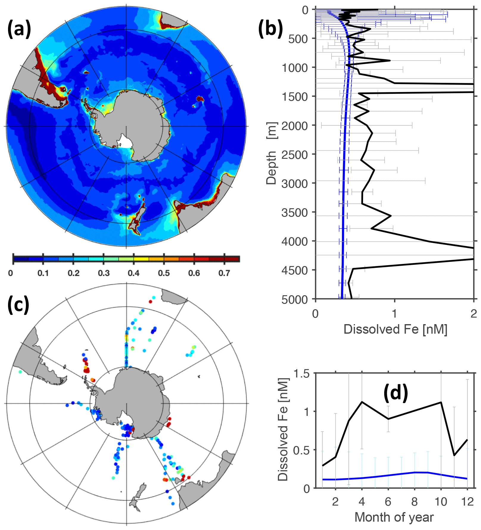
Figure 25 Comparison of simulated with observed dissolved iron concentrations. Panel (a) refers to simulated surface iron concentrations (reference simulation, averaged over nominal years 1993 to 1998). The color bar denotes iron concentrations in units of nM Fe. Panel (b) shows simulated (blue line) and observed (black line) concentrations averaged horizontally in the Southern Ocean (i.e., south of 40^∘ S), along with their respective spatial standard deviations (grey and blue horizontal bars). Panel (c) refers to observed surface iron concentrations (compiled by Tagliabue et al., 2012, and Mawji et al., 2014). (The color bar matches panel a.) Panel (d) depicts the simulated (blue line) and observed (black line) seasonal cycles of dissolved iron concentration at the surface calculated as monthly means averaged over the Southern Ocean.

The distribution of PO₄ and dissolved oxygen in the interior (cf. Figs. 26 and 27) is consistent with an overly vivid biological pump that is not throttled enough by iron limitation: a prolonged overestimated biological production drives an overly high export of organic matter to depth (cf. spurious PO₄ maximum around 400 m depth south of 60^∘ S). Once in the thermocline, this PO₄ is exported equatorwards and leaves the Southern Ocean (e.g., Marinov et al., 2006). Becoming part of the meridional overturning circulation, this excess PO₄ will return to the Southern Ocean at the surface. Because of insufficient iron limitation, the excess will be used up and exported to depth into, e.g., the Subantarctic Mode Water which leaves the Southern Ocean before it reaches higher latitudes. By this spurious mechanism, the Southern Ocean loses PO₄ to the rest of the world's ocean.

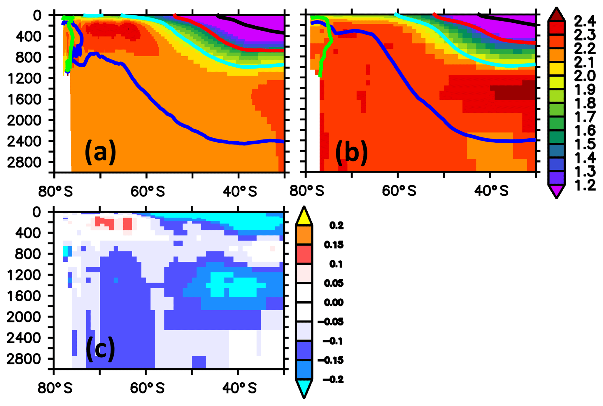
Figure 26 Zonally averaged meridional section of phosphate concentration in units of mmol P m⁻³. Panel (a) refers to simulated concentrations averaged over the nominal 1993–1998 period of the reference simulation; (b) refers to observed climatological concentrations (WOA09); (c) refers to the difference between simulated and observed concentrations, with blue colors denoting modeled concentrations that are biased low. The thick black, red, cyan, blue and green contours refer to mean densities (Sallée et al., 2013b, their Table 2) of subtropical water, mode water, intermediate water, circumpolar deep water and bottom water, respectively.

Figure 27 Zonally averaged meridional section of dissolved oxygen concentration in units of mmol O₂ m⁻³. Panel (a) refers to simulated concentrations averaged over the nominal 1993–1998 period of the reference simulation; (b) refers to observed climatological concentrations (WOA09); (c) refers to the difference between simulated and observed concentrations, with blue colors denoting modeled concentrations that are biased low. The thick black, red, cyan, blue and green contours refer to mean densities (Sallée et al., 2013b, their Table 2) of subtropical water, mode water, intermediate water, circumpolar deep water and bottom water, respectively.

The simulated patterns of dissolved oxygen bias in Fig. 27 are consistent with an overly efficient biological pump which strips the surface waters of PO₄ on their way from the world's ocean to higher latitudes, exports them to depth where they are remineralized and imprints a spurious oxygen deficit. Superimposed onto this, as a rough calculation suggests, is a negative bias of the order of 5 mmol O₂ m⁻³ caused by the temperature bias via the temperature dependence of oxygen solubility. Note that a more comprehensive analysis is beyond the scope of this model description which is intended to describe the configuration rather than evaluate it.

Figure 28 summarizes the model's fidelity in reproducing observed patterns of biogeochemical: ranked against the very similar, albeit coarser, non-eddying reference configuration used in Dietze et al. (2017) and UVic (here, referring to the reference version used in Löptien and Dietze, 2019, which is based on Keller et al., 2012), MOMSO appears to perform in a very similar manner.

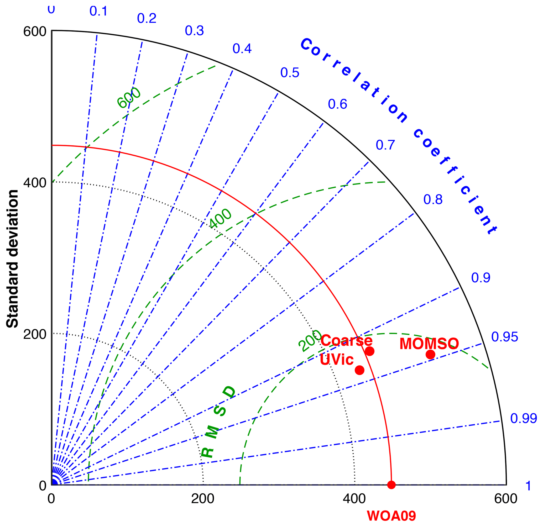
Figure 28 Taylor diagram of simulated phosphate concentration referenced to Southern Ocean WOA09 annual mean climatology (Garcia et al., 2010). The units for the standard deviation and root mean square deviations are µmol P m⁻³. “Coarse” refers to the very similar albeit coarser, non-eddying reference configuration used in Dietze et al. (2017) and “UVic” refers to the non-eddying Earth system model used, e.g., in climate engineering assessments (cf. reference version in Löptien and Dietze, 2019; Keller et al., 2012).

3.8 Computational cost

Initial development, testing and spin-up of the physical configuration was carried out on two 32-core workstations, based on a 6320 AMD Opteron (Abu Dhabi) (8-core CPU, 2.80 GHz, 16 MB L3 cache, DDR3 1600) interconnected with a QDR InfiniBand. As of 2013, the system cost ≈ EUR 10 000. The fully coupled ocean-circulation biogeochemical model has been run at a supercomputing center (project shk00027 at the Norddeutscher Verbund für Hoch- und Höchstleistungsrechnen, HLRN). Figure 29 documents excellent parallel performance up to 500 tasks – a setting which optimized our throughput on the machine/queueing system. On 500 Intel Xeon CPU E5-2670 cores (Sandy Bridge), it takes 10 h to simulate 1 year. Referring to pricing published by HLRN in 2018, this amounts to ≈ EUR 250 per integrated model year. We use compiler settings that optimize for maximum computational efficiency. They violate computational reproducibility (cf. Intel Fortran compiler option -fp-model and summary by Corden and Kreitzer, 2018). A description of the associated computational uncertainty is provided in Sect. 3.8 of Dietze et al. (2014), which uses the same code (applied to a different domain).

4 Research questions

The purpose of this section is to outline research questions for which MOMSO may serve as a tool. MOMSO is (to our knowledge) unique in that it (1) features a high spatial resolution in the Southern Ocean which allows an eddying circulation in combination with (2) a biogeochemistry that is sufficiently equilibrated such that the remaining trend is small enough to allows for studying decadal signals in SO carbon uptake; and (3) it is a “free-forward-in-time-running” model in a sense that (projected or hindcasted) anomalies to air–sea fluxes can be applied easily (as opposed to in data-assimilated or inverse models where this can be difficult). In the following, we sketch – very roughly – two ideas.

4.1 Wind-induced changes in Southern Ocean carbon uptake: parameterizing versus resolving the effects of eddies

Winds have been changing in the past decades over the Southern Ocean and they are anticipated to do so in the future. Lovenduski et al. (2013) estimate a linear increase at a rate of 14 % in 50 years throughout the period 1958 to 2007. Dietze et al. (2017) find in a coarse-resolution model that such a trend in winds is associated with a decreasing trend in Southern Ocean natural carbon uptake between 4.2 and 5.4 PgC 1000⁻¹ yr⁻² – depending on the choice of the underlying eddy parameterization. An open question is how these estimates compare against a model configuration that is actually resolving the eddying circulation rather than just parameterizing it. The main problem preventing an answer to this question so far has been the computational expense associated with running the carbon dynamics of a realistic eddying coupled ocean-circulation biogeochemical model into equilibrium.

MOMSO is identical to the coarse-resolution configurations used in Dietze et al. (2017), with the only difference being the higher spatial resolution and eddying circulation. Figures 13, 17, 30 and 31 show that the forcing of MOMSO with wind anomalies corresponding to a linear increase at a rate of 14 % in 50 years, as estimated by Lovenduski et al. (2013), drives trends in sea surface temperatures, sea surface salinities and the Eulerian overturning which are clearly distinguishable from the remaining model drift. In line with these clearly detectable trends in physical properties in response to increasing winds, Fig. 32 reveals that the associated trend in the oceanic uptake of natural carbon is also clearly detectable: the remaining drift in the MOMSO reference simulation is 1.0 PgC 1000⁻¹ yr⁻², allowing for a clear detection of the effect of increasing winds in simulation WIND which yields a substantially larger decline of 5.0 PgC 1000⁻¹ yr⁻².

Putting the simulated Southern Ocean carbon uptake in response to increasing winds into perspective, we find that MOMSO yields a drift-corrected 5 PgC 1000⁻¹ yr⁻² − 1 PgC 1000⁻¹ yr⁻²) = 4 PgC 1000⁻¹ yr⁻². Using the same code framework and exact same biogeochemical module (but much coarser spatial resolution), Dietze et al. (2017) find between 4.2 and 5.4 PgC 1000⁻¹ yr⁻² depending on the underlying eddy parameterization. So this is an indication that contemporary eddy parameterizations may provide results very similar to high-resolution eddying configurations.

Further investigations, which are beyond the scope of this sketch of a potential application of MOMSO, must include an in-depth analysis of eddy compensation, which is capable of canceling changes in wind-driven overturning (cf. Marshall and Radko, 2003; Viebahn and Eden, 2010; Abernathey et al., 2011, 2016; Hallberg and Gnanadesikan, 2006; Thompson et al., 2014; Tamsitt et al., 2017).

4.2 Wind-induced anomalies in Antarctic continental shelf bottom water temperatures

The realistic seabed temperatures (shown in Fig. 33), in combination with its biogeochemical module, provide a starting point which – with further development – may be suited to explore the following feedback loop with MOMSO: atmospherically driven changes in ocean-circulation drive additional heat supply which leads to basal melting. The buoyant lens of meltwater may, for one, suppress the AABW formation (Williams et al., 2016). This, in turn, affects oceanic carbon sequestration. Second, the meltwater carries bioavailable iron to the Southern Ocean – which affects oceanic primary productivity and the associated export of organic carbon to depth (Grotti et al., 2005; Lannuzel et al., 2008, 2010; Raiswell et al., 2008; Smith et al., 2007; Smith and Nelson, 1986; van der Merwe et al., 2009).

Figure 34 shows that the simulated Antarctic continental shelf bottom water (ASBW) changes its temperature in response to a linear wind increase (at rate of 14 % in 50 years, as estimated by Lovenduski et al., 2013). The magnitude of ASBW temperature is distinguishable from the persisting model drift in the reference simulation (cf. Fig. 34a, b) and simulated magnitudes are similar to recent observational estimates by Schmidtko et al. (2014) (cf. Fig. 34b, c). The sign, however, is reversed, which suggests that observed changes of ASBW temperatures cannot be attributed to the recent increases in wind strength alone. In any case, Fig. 34 suggests that the equilibration of the model has set in sufficiently so that model responses to decadal forcing variability are detectable.

5 Summary and conclusions

We set out to develop a near-global coupled ocean-circulation biogeochemical model which explicitly resolves effects of mesoscale eddy dynamics on the uptake of carbon in the Southern Ocean – in contrast to relying on respective eddy parameterizations. The setup is dubbed MOMSO, with MOM referring to the underlying framework (GFDL's Modular Ocean Model version MOM4p1) and SO referring to the Southern Ocean. We use the biogeochemical carbon module BLING developed by Galbraith et al. (2010).

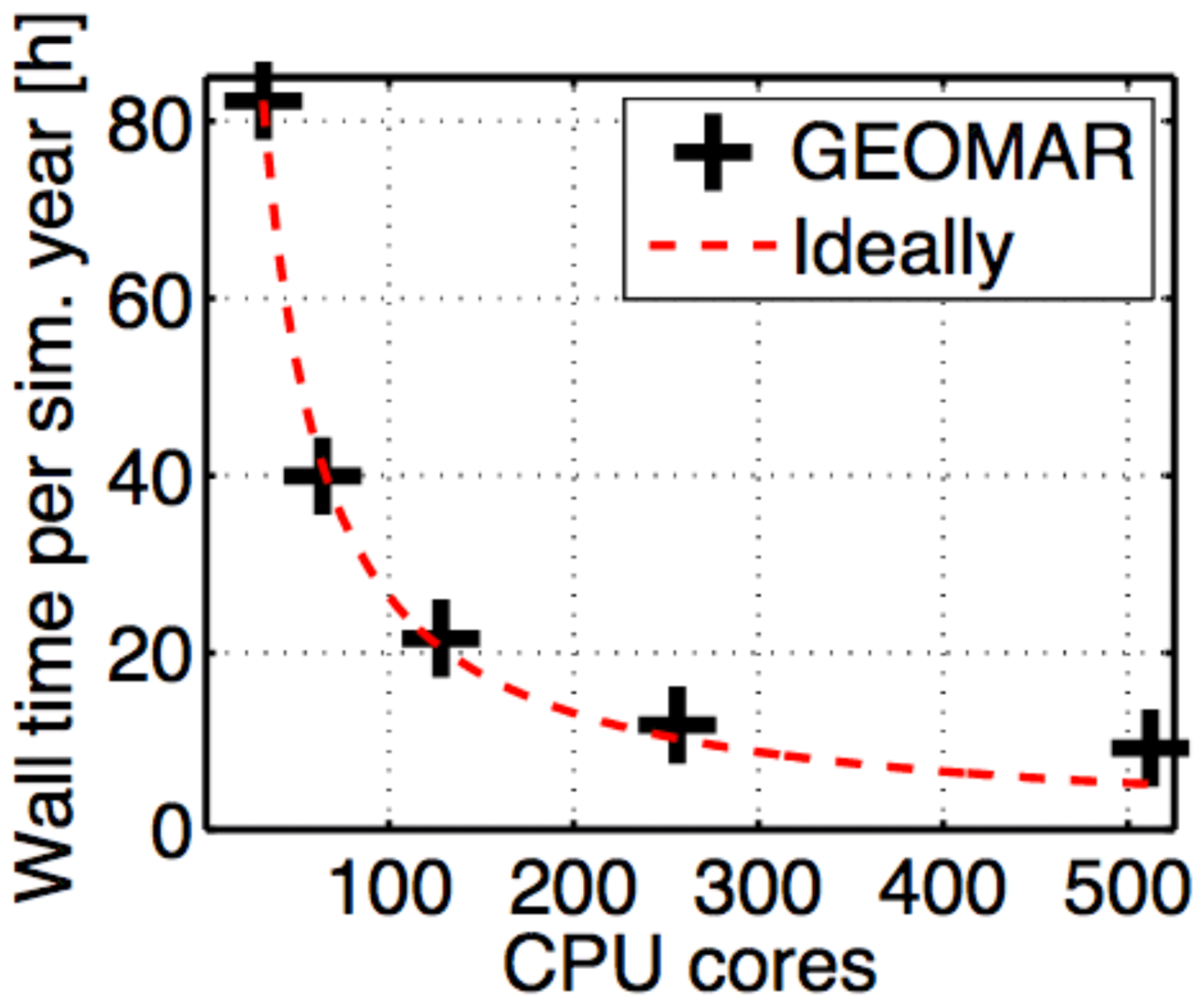
Figure 29 Computational performance as a function of CPU cores put to work simultaneously. On 500 Intel Xeon CPU E5-2670 cores, it takes 10 h to simulate 1 year.

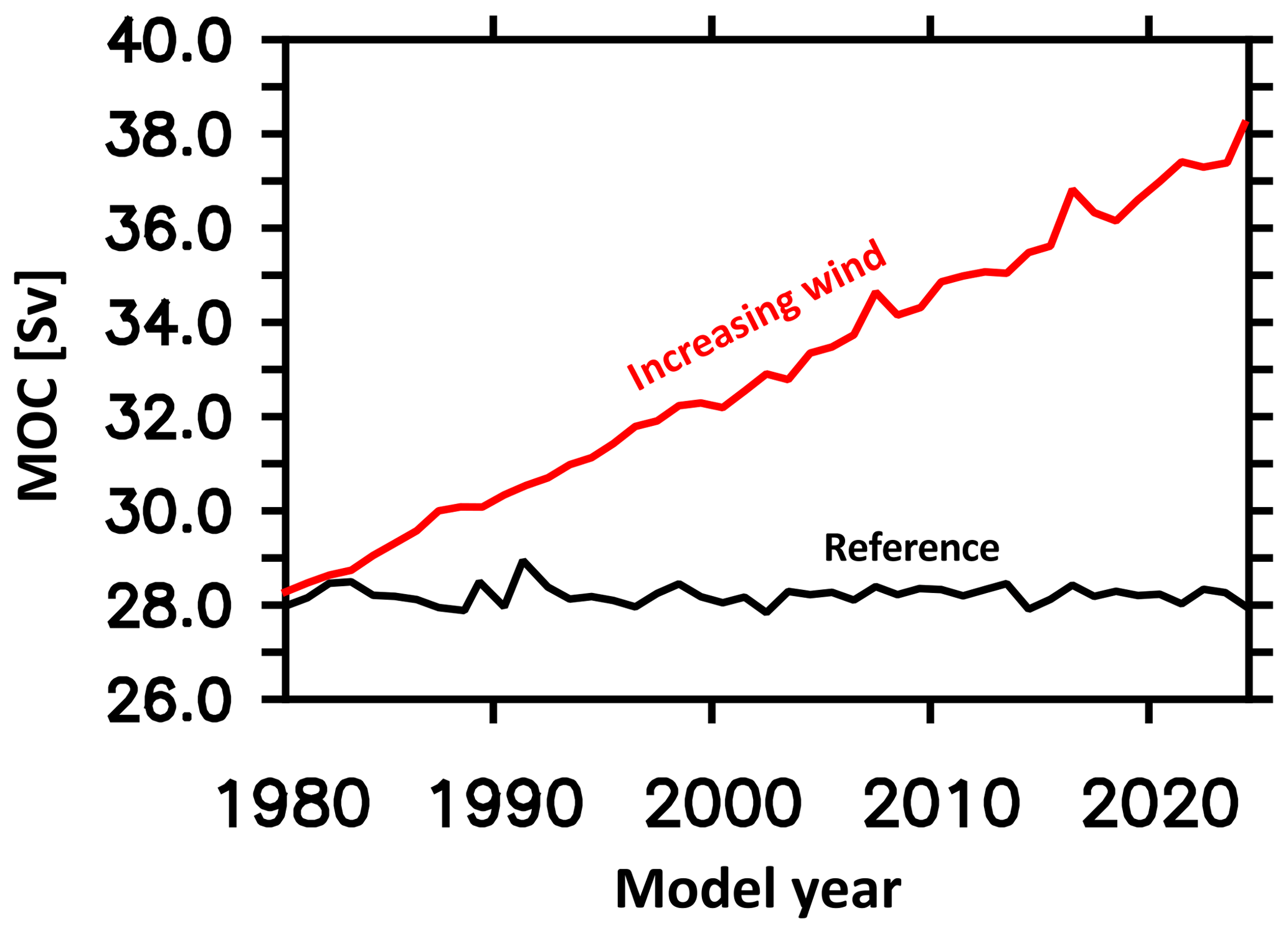
Figure 30 Maximum Southern Ocean Eulerian meridional overturning circulation south of 40^∘ S in units of 10⁶ m³ s⁻¹. The black (red) line refers to the reference (increasing wind) simulation.

Overall, we find in a climatological simulation (REF) an eddying surface circulation that is in reasonable agreement with observations from space. Further, simulated temperatures and sea surface salinity show a close agreement with observations. Sea ice cover is biased high but is still in the range of observed values during particularly cold winters. A remaining caveat is a low bias in the Drake Passage (99 Sv compared to observational estimates ranging from 110 to 170 Sv). This may be associated with locally enhanced viscosity over rough topography at the exit of the Drake Passage (cf. Fig. 2) which has been necessitated by numerical stability. (Whether this is associated with our very low choice of the Smagorinsky isotropic viscosity and/or the lack of biharmonic viscosity/diffusion as suggested by reviewer 1 still warrants investigation.)

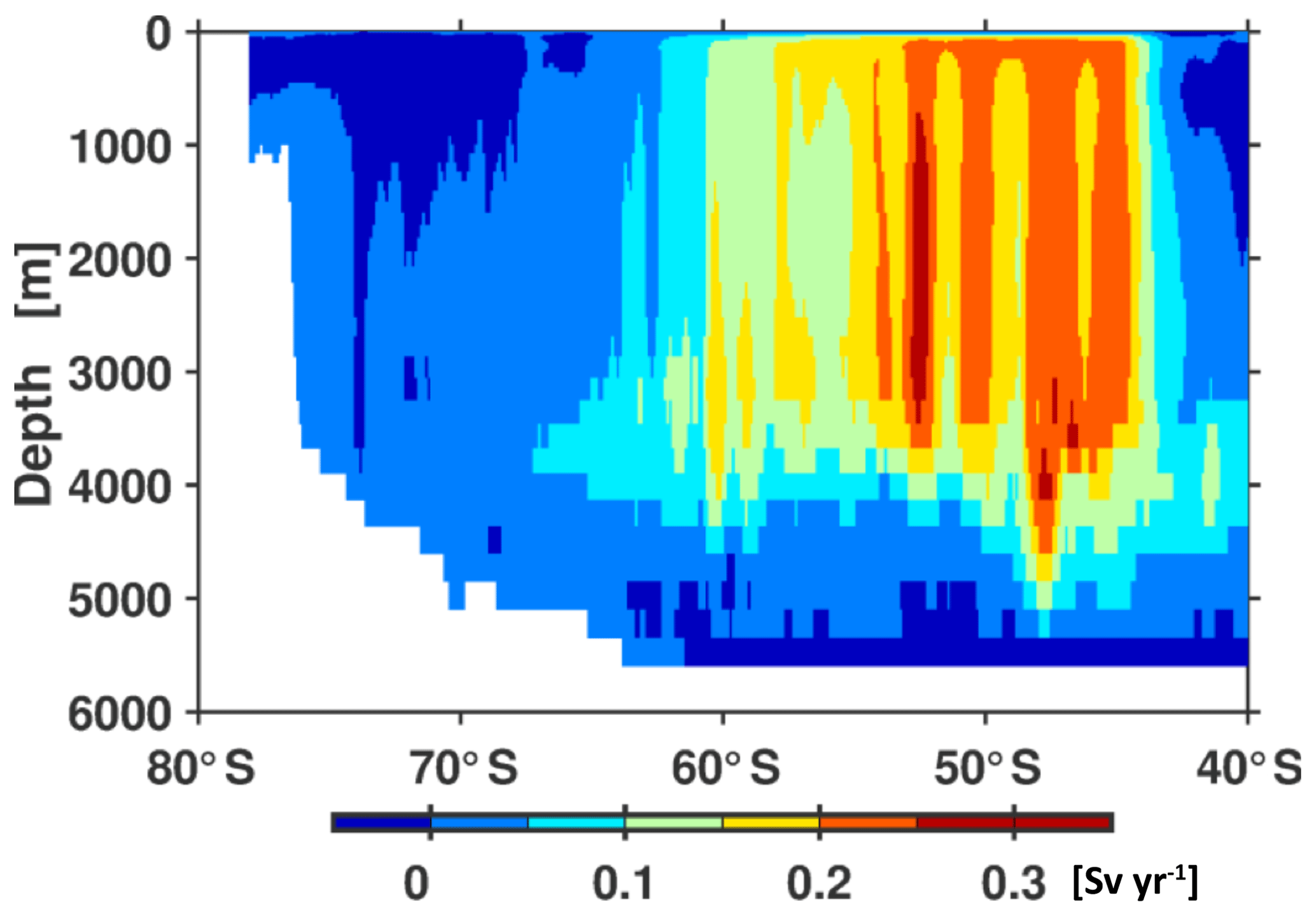
Figure 31 Simulated linear trend of Southern Ocean Eulerian meridional overturning circulation effected by increasing winds during nominal years 1980 to 2024 in units of 10⁶ m³ s⁻¹ yr⁻¹. Positive values denote increasing overturning.

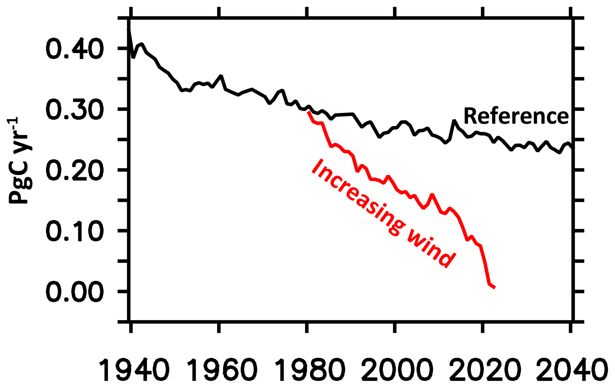
Figure 32 Simulated oceanic uptake of natural carbon south of 40^∘ S. The black (red) line refers to the reference (increasing wind) simulation.

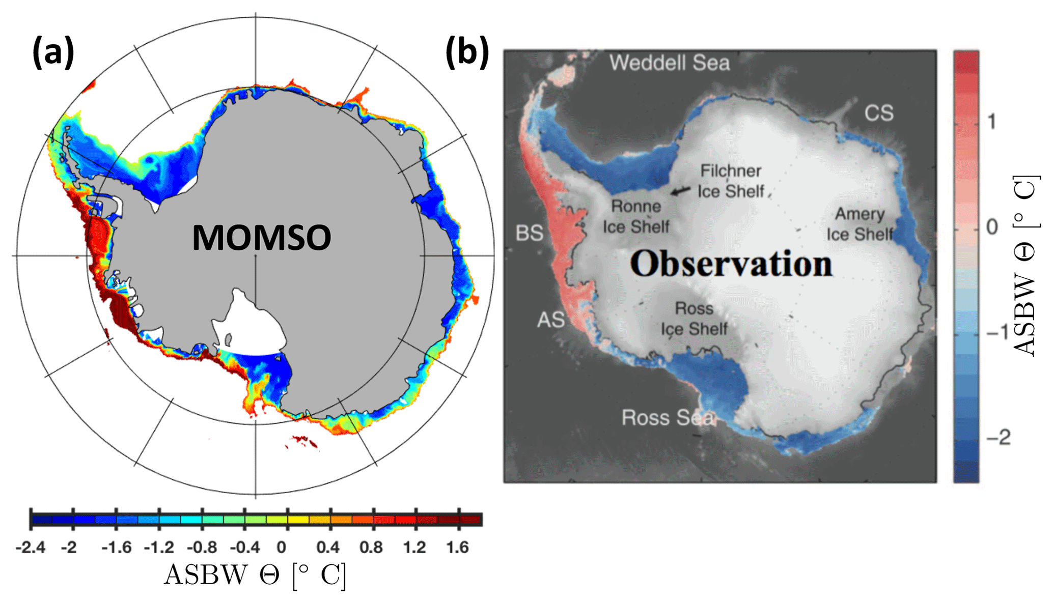
Figure 33 Temperature of ASBW at the seabed for depths shallower than 1500 m. Panels (a) and (b) refer to the simulated 1993–1998 climatology and observations reproduced from Schmidtko et al. (2014), respectively.

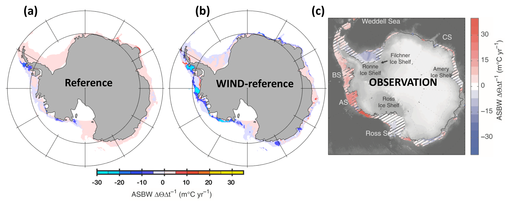
Figure 34 Temporal trend in the temperature of the ASBW at the seabed for depths shallower than 1500 m. Panel (a) refers to the drift that is still persistent in the reference simulation during nominal years 1980–2024. Panel (b) refers to the trend in simulation in the simulation with increasing winds corrected by the drift that still persists in the reference. Panel (c) refers to an observational estimate reproduced from Schmidtko et al. (2014).

The simulated biogeochemistry is also biased. Surface PO₄ concentrations are too low in the Southern Ocean, which is indicative of a deficient formulation of the limitation of phytoplankton growth. Seasonally varying biases in simulated surface iron concentrations suggest that the problem is associated with an up-to-date, incomprehensive quantitative understanding of iron dynamics. The model performance with respect to biogeochemistry is, however, similar to what the state of the art is in coarse-resolution models.

MOMSO is a step forward in the field of eddying coupled ocean-circulation biogeochemical carbon modeling in that it allows to investigate the effects of decadal changes in atmospheric boundary conditions on the oceanic carbon uptake with an eddy-resolving model that features a realistic geometry and topography. Previous attempts have been hindered by the computational cost that is associated with running simulations into a semi-equilibrated state which features trends considerably lower than the climate signals (as affected by prescribed anomalies in boundary conditions) under investigation. To this end, MOMSO benefitted from (1) an ever-increasing ease of access to computing power that is associated with Moore's law and (2) the fortunate coincidence that the spun-up coarse-resolution restart from Dietze et al. (2017) was close enough to the equilibrated high-resolution state of MOMSO such that it provided a relatively equilibrated starting point.

In this model description paper, we showcased that the remaining drift in MOMSO's Southern Ocean carbon uptake is substantially lower than changes driven by typical decadal variability of atmospheric variations. We illustrate that the respective sensitivity experiment is suitable for a comparison to coarser-resolution model versions and present a first impression in Fig. 32. Similarly, we find that the drift in simulated temperatures of the ASBW is small enough to allow to link atmospheric decadal variability to oceanic temperature variations at the boundary to ice shelves around Antarctica.

We illustrate that the respective sensitivity experiment is suitable for a comparison to coarser-resolution model versions and present a first impression in Fig. 25.

On a final note, the computational cost associated with integrating MOMSO is substantial. With present-day hardware, full spin-ups are in the five-figure Euro range so that extensive tuning of the biogeochemical model, which still features some substantial misfits to observations, is uneconomical. Starting from the already spun-up state presented here, however, is in the reasonable range of EUR 2500 per decade. The corresponding energy needs (operation only) are of the order of 1000 kWh per decade. Using a carbon intensity of 450 gCO₂ kWh⁻¹ (e.g., Moro and Lonza, 2018), this yields an emission of around 0.5 t of CO₂ per simulated decade.