TITAM (v1.0): the Time-Independent Tracking Algorithm for Medicanes

This work aims at presenting TITAM, a time-independent tracking algorithm specifically suited for medicanes. In the last decades, the study of medicanes has been repeatedly addressed given their potential to damage coastal zones. Their hazardous associated meteorological conditions have converted them to a major threat. Even though medicane similarities to tropical cyclones have been widely studied in terms of genesis mechanisms and structure, the fact that the former appear in baroclinic environments, as well as the limited extension of the Mediterranean basin, makes them prone to maintaining their warm-cored and symmetric structure for short time periods. Thus, the usage of a measure for the warm-core nature of the cyclone, namely the Hart conditions, is a key factor for successful identification of a medicane. Furthermore, given their relatively small spatial extent, medicanes tend to appear embedded in or to coexist with larger lows. Hence, the implementation of a time-independent methodology, avoiding the search for a medicane based on its location at previous time steps, seems to be fundamental when facing situations of cyclone coexistence. The examples selected showcase how the algorithm presented throughout this paper is useful and robust for the tracking of medicanes. This methodology satisfies the requirements expected for a tracking method of this nature, namely the capacity to track multiple simultaneous cyclones, the ability to track a medicane in the presence of an intense trough inside the domain, the potential to separate the medicane from other similar structures by handling the intermittent loss of structure, and the capability to isolate and follow the medicane center regardless of other cyclones that could be present in the domain. The complete TITAM package, including preprocessing and post-processing tools, is available as free software extensively documented and prepared for its deployment. As a final remark, this algorithm sheds some light on medicane understanding regarding medicane structure, warm-core nature, and the existence of tilting.

1 Introduction

Cyclones can be broadly classified in terms of their thermal character as cold-core or warm-core (Hart, 2003). Those developing in middle and high latitudes are cold-core and obtain their energy from the baroclinic instability typical of these latitudes. Instead, warm-core cyclones develop in tropical and subtropical zones and, according to the latest theories (Zhang and Emanuel, 2016; Emanuel, 1986), are powered by enthalpy fluxes and maintained by self-induced heat transfer from the ocean (WISHE theory); “self-induced” makes reference to winds associated with the cyclone. However, this conceptual framework, which considers two completely different types of storms, is a major simplification of real cyclones. Actual storms have a variable degree of similarity between these two idealized models, and indeed they evolve by changing their thermal structure during their lifetime (Hart, 2003).

One particular type of storm is a medicane (from Mediterranean hurricanes), which does not perfectly fit either of these two idealized models. Medicanes are meteorological mesoscale systems formed in the Mediterranean basin, where baroclinicity provides the necessary atmospheric instability for the formation of cyclones. Under certain circumstances, the environment favors the tropical transition of a storm, creating a spiral band of clouds around a well-defined cloud-free eye, while showing thermal symmetry and a warm core. The “tropical-like” term is introduced to account for the fact that, although they share similar mechanisms with tropical cyclones, they develop beyond the tropics (Homar et al., 2003; Gaertner et al., 2018).

According to the classical theory of tropical cyclone formation, a sea surface temperature (SST) above 26 ^∘C (Palmén, 1948; Emanuel, 2003; Tous and Romero, 2013) is necessary for tropical cyclogenesis. In the absence of baroclinicity, a high SST is needed so that the lapse rate forces the atmosphere to be unstable enough for convection (Stull, 2017, chap. 16). However, the intrusion of a cold cutoff trough in upper levels, which causes cool air temperatures at high altitude, can trigger convection and lead to tropical cyclogenesis even when waters are not warm enough (McTaggart-Cowan et al., 2015). Hence, the fact that the presence of Mediterranean tropical-like cyclones is associated with cold-air intrusions explains why they can form even when the SST is below 26 ^∘C (Miglietta et al., 2011).

Midlatitude cyclones with tropical characteristics and actual tropical cyclones show similar but slightly different characteristics. Their main similarities are their appearance in satellite images, showing an eye in their structure, and their dynamical and thermodynamic features: a warm-core anomaly decreasing with altitude, weak vertical wind shear, strong rotation around the pressure minimum (high low-level vorticity), and convective cells organized in rainbands extending from the eye wall (Miglietta and Rotunno, 2019). The largest differences in medicanes and tropical storms pertain to the intensity and duration. Medicane lifetime is restricted to a few days due to the limited extent of the Mediterranean Sea, and they attain their tropical character only for a short period, while retaining extratropical features for most of their lifetime; the horizontal extent is generally confined to a few hundred kilometers and the intensity rarely exceeds Category 1 of the Saffir–Simpson scale (Miglietta et al., 2011; Miglietta and Rotunno, 2019). Thus, while tropical cyclones can reach a radius of 1000 km, 910 hPa minimum central sea level pressure (SLP), and 295 km h⁻¹ maximum 1 min sustained winds (Anthes et al., 2006; Shen et al., 2006), their Mediterranean counterparts show a smaller radius (up to 150 km) (Tous and Romero, 2013), a less intense central SLP minimum (980 hPa), and slower winds (gusts of about 180 km h⁻¹) (Nastos et al., 2015; Miglietta et al., 2013).

In the literature, detection and tracking methods for tropical cyclones are extensive. Some of them serve as a good base for the development of a medicane tracking algorithm, especially those applying a time-independent methodology. Hodges (1994) presented a first work on an automated tracking method with general application to a wide range of geophysical fields. It is based on an identification of feature points by segmentation of structures and a further decomposition and analysis of the different structure points. The tracking part is based on former works (Salari and Sethi, 1990; Sethi and Jain, 1987) and consists of a constrained optimization of a cost function to determine the correspondence between the found feature points. Blender et al. (1997) succeeded in introducing a time-independent tracking method with few constrictions in order to allow maximum applicability, including a further discussion on its validity for different spatial and temporal resolutions of the model data (Blender and Schubert, 2000). Vitart et al. (1997) also introduced an objective procedure for tracking model-generated tropical storms similar to the one described by Murray and Simmonds (1991) using a time-independent approach. The same basic two-step methodology introduced in these works has been described in later works. Included among these is the one by Bosler et al. (2016), which addresses the issue of measuring distances at high latitudes by using geodesic distance instead of geometric distance between points. Also included in this set is one contribution by Wernli and Schwierz (2006), in which, in addition to a tracking algorithm, a new method for identifying cyclones and their extent is presented, being particularly useful for cyclonic climatological studies. Ullrich and Zarzycki (2017) argue that “uncertainties associated with objective tracking criteria should be addressed with an ensemble of detection thresholds and variables, whereas blind application of singular tracking formulations should be avoided”, and they provide a tool for tracking tropical and extratropical cyclones, along with easterly waves. Kleppek et al. (2008) employ “the standard method for midlatitudes” (Blender et al., 1997) and add the relative vorticity at 850 hPa to the center identification variables to address the difficulty of tropical cyclones not being detected during genesis, decay, or landfall stages. Other related works include the following: Raible et al. (2008), which presents a comparison of detection and tracking methods (Blender et al., 1997; Wernli and Schwierz, 2006; Murray and Simmonds, 1991) for extratropical cyclones employing different reanalyses; Zhao et al. (2009), adapting the earlier work by Vitart et al. (1997) and applying it to a climatology of global hurricanes in a 50 km resolution GCM; and Horn et al. (2014), who study the dependence of a simulated tropical cyclone in climate model data on three tracking schemes (Walsh et al., 2007; Zhao et al., 2009; Camargo and Zebiak, 2002). The contribution by Hanley and Caballero (2012) is also worth mentioning, who succeed in the implementation of a novel method for recognizing “multicenter cyclones”, which is one of the main objectives of the present work, and even properly handling cyclone merger and splitting events; however, this method seems to rely solely on SLP, an important caveat when the objective is the isolation of warm-core cyclonic systems. In general, although these methods are useful for tropical cyclones, with some of them even being designed for a more general cyclone range, the particular case of medicanes shows important drawbacks, namely their coexistence with close extratropical lows, their temporal loss of the warm-core nature due to vertical tilting, and their weak character when compared to genuine tropical cyclones.

Despite their similarities to tropical cyclones, there seems to be no agreement on the best algorithm to be used for the tracking of medicanes (Tous and Romero, 2013; Picornell et al., 2014). Concerning medicane tracking methods, some of them are designed to select a first track point and calculate its movement direction from the different meteorological fields, along with some conditions that should be satisfied. This approach directly limits the applicability of the method, as it is affected by a strong dependence on the initial tracking time (Hart, 2003). Thus, a time-independent tracking method seems necessary for medicanes.

An additional problem is related to the detection of simultaneous storms. While very uncommon, particularly when the considered domain is carefully chosen, the real coexistence in time of two medicanes inside a domain could happen, and the ability to capture more than one medicane may then be of utmost importance. Indeed, searching for two medicanes is technically the same as searching for two low-pressure areas, and then the ability to handle multiple structures becomes essential to avoid the risk of systematically tracking the one with the lowest pressure instead of the one being a medicane. The Hart parameters (Hart, 2003), which will be explained later, are derived variables used to characterize the thermal nature of the cyclone by means of the Hart conditions, used herein to find warm-core structures.

Thus, without overlooking the advantages of making progress toward a precise medicane definition or the study of their genesis and maintenance in terms of dynamical and thermodynamical mechanisms, the main efforts of this work have been aimed at developing a tracking algorithm allowing the coexistence of multiple storms of this nature. In this way, even in the absence of an optimal medicane definition, the flexibility provided by a parameter-oriented methodology favors the detection of this type of storm within a reasonable range of the parameters leading to that definition. As a previous step to introducing the designed algorithm, a brief review on the existing methods for tracking cyclones that are suitable for medicanes is carried out below and summarized in Table 1.

Alpert et al. (1990)Picornell et al. (2001)Hart (2003)Suzuki-Parker (2012)Marchok (2002)Cavicchia and von Storch (2012)Zahn and von Storch (2008b)Sinclair (1994)Walsh et al. (2014)

Table 1 Summary of some cyclone tracking methods usually applied to medicanes.

Picornell et al. (2001) introduce a widely used methodology for mesocyclone detection and tracking based on four steps: they first locate all the pressure-relative minima as potential cyclones in each analysis, then filter them by imposing a minimum pressure gradient of 0.5 hPa∕100 km along at least six of the eight directions. Another filter based on the distance between two potential cyclones is applied too, taking the one with the largest circulation in the case that they are closer than four grid points. Finally, they apply a methodology to calculate the track based on the hypothesis that the 700 hPa level is the steering level of the movement of a cyclone (Gill, 1982), thereby considering the wind at that level to determine the direction in which the cyclone will preferably move. The methodology described in Alpert et al. (1990), based on a search for the track oriented within an ellipse whose major axis is defined by the 700 mb wind vector, is then extended with the definition of two additional elliptical areas in which the search for a storm center in the following time steps is performed. A disadvantage of this approach when applied to medicane detection lies in the selection of a single point as the medicane center before checking the warm–cold nature of the cyclone. As we demonstrate below with an example, there may be a little tilting in the medicane structure, leading to a displacement between the points fulfilling the Hart conditions, detailed in Sect. 3.3.1, and the points showing the minimum surface pressure or cyclonic vorticity. If this were the case, then the track could suffer from an artifact loss of the tropical cyclonic nature when trying to impose the Hart conditions to the minimum pressure point of a tilted structure. This is also discussed in Hart (2003), along with the convenience of using either mean sea level pressure (MSLP) or vorticity for the identification of the cyclone center.

The methodology introduced by Hart (2003) has been widely applied in the years since its publication. It consists of making a time-dependent track by finding a first track point and identifying the consecutive track points through a series of conditions based on center spatial and temporal displacement. Despite the difficulties that this method may face, its simplicity makes it very useful, and it has been used in this work as detailed below. In the same work, a phase space based on a set of parameters is proposed to determine the thermal nature of a cyclone. These parameters are thoroughly revisited in this contribution and have great significance in the proposed method.

In a similar approach, Suzuki-Parker (2012) develop a tracking procedure dependent on the previous time step. The authors introduce previous filters by imposing thresholds in the 850 hPa wind speed, cyclonic relative vorticity, and horizontal temperature anomalies.

Nevertheless, algorithms based on the search for a new track point depending on the previous point show important disadvantages for the purpose of tracking multiple cyclones at a time. Regardless of the criteria used to confine the search area for the next point, they are designed to find one single cyclone path and show a strong dependence on the first chosen time step. In fact, this problem is clearly stated in Hart (2003), wherein the reader is warned about this possible effect. The problem of tracking a cyclone by using its location in the previous time step is illustrated below through an example.

There are more advanced tracking methods, such as the one suggested by Marchok (2002) based on Barnes interpolation of seven different fields, namely the SLP, 700 and 850 hPa relative vorticities, 700 and 850 hPa geopotential heights, and two secondary parameters (minimum wind speed at 700 and 850 hPa). This method has been implemented in the operational NCEP (National Centers for Environmental Prediction, operated by NOAA) cyclone tracking software.

Cavicchia and von Storch (2012) apply a tracking methodology based on previous works (Zahn and von Storch, 2008b, 200a) and on the identification of the pressure minima as potential centers as well as the subsequent clustering relying on the distance between them. This method is very close to the one presented here in the concept of finding center candidates as independent entities, but it shows a disadvantage: the pressure minimum, as shown below, is not always the best choice for the medicane center. A different field is introduced here with the purpose of preventing this pitfall. Additional factors are considered to filter the center candidates, such as the Hart conditions and the symmetry of the geopotential height gradient.

Sinclair (1994) analyzes the limitations and benefits of using either SLP or vorticity for tracking. As detailed below, both parameters are indeed used by the method we propose in this work to isolate the potential medicane centers.

Walsh et al. (2014) use both SLP and cyclonic vorticity to find medicane centers. Afterwards, temperature anomalies in the center are calculated to study the warm-core nature of the cyclone. However, in the same way as in the previously mentioned methods, the selection of a single point could produce gaps in the tracks. This effect is acknowledged in their text and could be diminished by the multicandidate selection and clustering method proposed here.

Here a new methodology for tracking medicanes is presented. It overcomes the drawbacks of previous methods. This new methodology does not need an initial state of the medicane, is able to identify various simultaneous structures, and prevents the aforementioned loss of structure. Also, its parallel performance (see Appendix C for details) enables its application to long-term simulations.

2 Preprocessing: building the input data

The total tracking procedure consists of a first step for preparing the input data, a second step with the execution of the algorithm, and a final post-processing of the output data provided by the algorithm.

The input data for the algorithm consist of files containing temporal series of a number of meteorological fields. The mandatory 2D and 3D fields are SLP, 10 m wind horizontal components (U10, V10), and geopotential height (Z) for at least the 900, 800, 700, 600, 500, 400, and 300 hPa levels.

The input provided by the user must be compliant with the specifications given in Appendix B regarding the input format, the internal name of the variables and dimensions, the physical units, and the order of the matrices. Note that the algorithm package includes a preprocessor for Weather Research and Forecasting (WRF) model output called “pinterpy” (more details in Appendix B).

3 Medicane tracking algorithm

TITAM is rather complex and consists of several steps, so the main components are briefly outlined here, while the details of each part are thoughtfully described into the following subsections (Fig. 1). Overall, the algorithm can be divided in two main blocks: the detection of the cyclone (medicane) centers in each time step (red box in Fig. 1) and the creation of a track by joining the centers through the time domain (D).

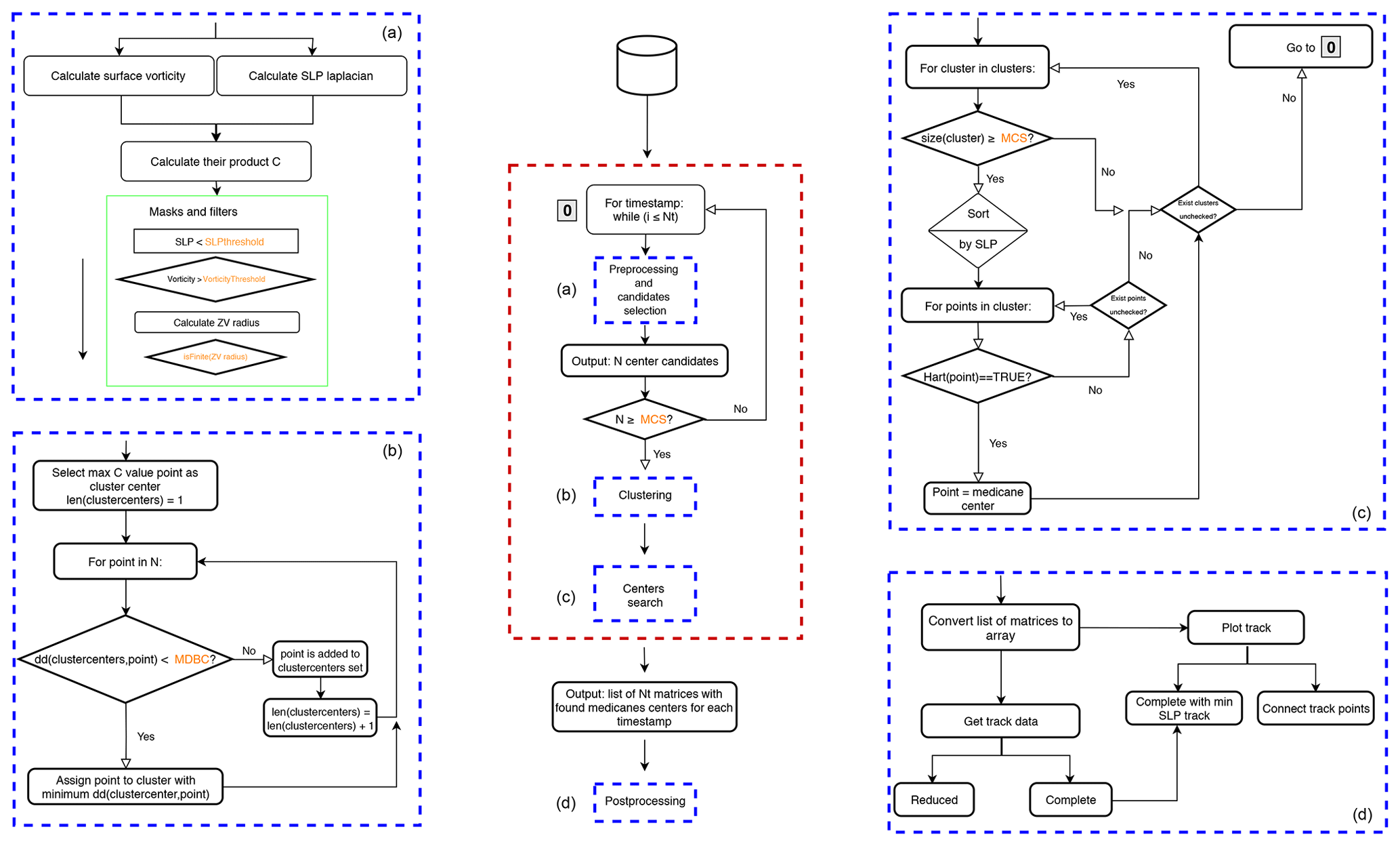
Figure 1 Flowchart describing the algorithmic implementation for the proposed medicane detection methodology TITAM (for the medicane detection part). MCS and MDBC correspond to the MinPointsNumberInCluster and SLPminsClustersMinIBdistance algorithm parameters, respectively.

The detection block consists of three main steps. In the first part, (A) the algorithm makes a first selection of the potential candidates for medicane centers. Once the candidates are selected, (B) they are grouped using an ad hoc clustering method. Each group eventually leads to a potential cyclone. Finally, (C) the algorithm searches for a center of the cyclone by verifying the thermal conditions for being a medicane, i.e., the Hart conditions, explained below. The search for centers is carried out for each time step separately and regardless of their location in the previous step. This allows us to benefit from a key feature of the algorithm: time independence. It enables a straightforward parallelization in the code implementation (see Appendix C for details).

In the second block (D), the points resulting from the procedure above, which are not yet connected in space or time, get linked following a set of rules. The details are given in Sect. 3.4.

3.1 Searching for center candidates (A)

3.1.1 Filtering by cyclonic potential, SLP, and vorticity

The first step is to define a diagnosed field acting as an indicator of areas with high vorticity and revealing a minimum in the pressure field, i.e., those prone to cyclonic activity. The selected variables are 10 m relative vorticity and SLP Laplacian. Using the product of these two fields emerges as a good strategy for finding the candidate points. This magnitude brings out all the points being SLP minima with high cyclonic character. This diagnosed field, hereafter referred as cyclonic potential C, is thus defined as

$$\begin{array}{}\text{(1)}& \mathbf{C}={\mathrm{\nabla }}^{\mathrm{2}}\left(\mathbf{SLP}\right)\cdot {\left(\mathbf{\nabla }\times {\mathit{v}}_{\mathrm{10}}\right)}_z,\end{array}$$

where the dot represents a Hadamard product, and the z subscript means that only the z component of the surface wind curl (i.e., the surface vorticity) is considered. Given this definition, a high positive value of C at a given point reveals the cyclonic nature of the flow around it. The definition of C is motivated by the relationship between the geostrophic relative vorticity and the Laplacian of the pressure field obtained within the context of the quasi-geostrophic theory; this is

$$\begin{array}{}\text{(2)}& {\mathit{\xi }}_{\mathrm{g}}={\displaystyle \frac{\mathrm{1}}{{\mathit{\rho }}_{\mathrm{0}}f}}{\mathrm{\nabla }}_{\mathrm{h}}^{{}^{\mathrm{2}}}p,\end{array}$$

where ξ_g is the geostrophic relative vorticity, ρ₀ and f are constants, and ∇_h is the horizontal gradient operator at a fixed height (Holton and Hakim, 2012). Hence, the product represented by C would be redundant if the 10 m wind field was well represented by the geostrophic wind approximation at the surface level. Nevertheless, for a medicane, large surface effects are present and the surface wind is thus not well represented by the geostrophic approximation. Indeed, from this point of view this product is expected to have a greater benefit with respect to using the SLP alone in those cases in which SLP perturbations occur due to orographic factors.

Once C is calculated, this field is successively 1–2–1 smoothed N times (see parameter SmoothingPasses in Appendix A). This filter is necessary because of the noisy character of the SLP Laplacian in high-resolution data. The next step is to filter out all the grid points with an SLP value above a certain threshold (see parameter SLPThreshold in Appendix A), and those with a C value above the threshold marked by a given percentile (99.9 by default; see parameter ProductQuantileLowerLimit in Appendix A) are retained. On the other hand, a review of the vorticity values exhibited in the different medicane simulations suggests that a lower threshold of 1 rad h⁻¹ is enough to filter out the situations in which no medicanes are present (see parameter VorticityThreshold in Appendix A). Therefore, points with lower cyclonic potential are removed following the above criteria. Note that, with the provided definition of vorticity, it is dependent on the horizontal grid spacing, and henceforth the provided default value for the vorticity threshold may not be suitable for cases with different horizontal grid spacings.

3.1.2 Symmetry and radius

The next step consists of applying a filter to remove candidates for the cyclone center based on the symmetric structure and radius of the medicane. Any point not satisfying both conditions is discarded as a center candidate. The horizontal domain of a cyclone is defined as the area of positive vorticity around the cyclone center, bounded by the zero-vorticity line (Picornell et al., 2001; Radinovic, 1997). This domain, which should be quasi-symmetric in the case of a medicane, is used to define the medicane effective radius (MER). The zero-vorticity radius is defined as the distance from the candidate point to the points at which vorticity changes its sign from positive to negative (see parameter CalculateZeroVortRadiusThreshold in Appendix A). In our case it is calculated for eight angular directions (every π∕4 radians). The MER is then estimated as the mean of the eight zero-vorticity radiuses. This calculation is conditioned by the number of points considered for performing the sign change search over each direction, which is equivalent to the maximum distance tested (see parameter CalculateZeroVortRadiusDistance in Appendix A).

Conditionally (see parameter IfCheckZeroVortSymm in Appendix A), we can check the symmetry of the zero-vorticity line. Firstly, we impose the requirement that the zero-vorticity radius must exist for a minimum number of the eight directions tested (see parameter ZeroVortRadiusMinSymmDirs in Appendix A). Next we define the asymmetry coefficient A_c as the maximum difference of the eight calculated radiuses. The candidate point is rejected as such if A_c>A_p, where A_p is an algorithm parameter (see parameter ZeroVortRadiusMaxAllowedAsymm in Appendix A). Finally, to keep the candidate point, we impose the calculated MER to be in a range of possible radiuses: maximum MER_H and minimum MER_L (see parameters ZeroVortRadiusUpperLimit and ZeroVortRadiusLowerLimit in Appendix A). These parameters must be set by the user based on the typical observed values for MERs. The points discarded by this filter are mainly orographic artifacts that tend to appear due to orography-induced vorticity. Note that this condition of symmetry of the zero-vorticity radius is similar to that of the SLP gradient in multiple directions used by other authors (e.g., Picornell et al., 2001; González Alemán, 2019; Cavicchia and von Storch, 2012). The main difference lies in the fact that they impose a lower limit for the SLP gradient in the different directions but do not check the difference in magnitude across gradients.

A consistent calculation of this zero-vorticity radius is of great importance, as it will serve as the radius to calculate the Hart parameters for the points held as center candidates after the filters. Defining a variable radius that depends on the situation rather than a constant unique value is a flexible solution that overcomes the problem of dealing with very different structures in the same domain (Cioni et al., 2016; Picornell et al., 2014; Chaboureau et al., 2012; Miglietta et al., 2011).

3.2 Grouping potential centers (B)

As previously mentioned, the advantage of allowing multiple center candidates is the possibility of finding a medicane center being neither the absolute SLP minimum nor the point with a maximum value of C, as those could not fulfill the thermal structure of warm-core cyclones. On the other hand, the algorithm should ideally have the ability to find multiple concurrent cyclones. To achieve these requirements, we separate the center candidates into different clusters. Note that the number of points passing the previous filters must be above the number of points marked by the parameter MinPointsNumberInCluster.

The cluster classification is built upon a distance d_c that marks the minimum separation distance between two cluster representative points (see parameter SLPminsClustersMinIBdistance in Appendix A). This parameter should be set taking into account the common range within which a medicane radius usually lies. The clustering method is a reduced k-means clustering without iterative calculation, in which the number of groups (see parameter MaxNumberOfDifferentClusters in Appendix A) is computed as the number of center candidates separated by more than the distance d_c from the other candidates. The cluster centers are selected by C value: the point with the highest 𝒞 is selected as the center; the second one is selected as the center if the distance is higher than SLPminsClustersMinIBdistance, and so on. Imposing an upper limit for the number of clusters prevents the inclusion of clusters not being real medicane candidates in large domains, especially if the values selected for the previous filters were not tight enough.

The final task of the grouping method is to filter out all the points belonging to clusters formed by fewer than a minimum number of points (see parameter MinPointsNumberInCluster in Appendix A). These clusters are considered to be too small to constitute a medicane structure, and hence their points are discarded as center candidates.

3.3 Identification of warm-core structures (C)

The final list of center candidates is composed of points that pass all the filters and conditions, showing a high cyclonic character and a high symmetry in the zero-vorticity line enclosing the medicane domain, as well as pertaining to a cluster made up of enough candidates to be considered a medicane structure.

3.3.1 Hart conditions

The thermal nature of a cyclone is customarily studied through the so-called Hart parameters (Hart, 2003). Based on these parameters, the Hart conditions are described regarding the existence of a thermal symmetry around the center and the warm-core character of the cyclone nucleus. These two features define the nature of a tropical cyclone. The former is evaluated by means of a symmetry parameter B, defined as

$$\begin{array}{}\text{(3)}& B=h\left(\stackrel{\mathrm{‾}}{{\mathbf{Z}}_{\text{600\hspace{0.17em}hPa}}-Z_{\text{900\hspace{0.17em}hPa}}}{|}_R-\stackrel{\mathrm{‾}}{{\mathbf{Z}}_{\text{600\hspace{0.17em}hPa}}-Z_{\text{900\hspace{0.17em}hPa}}}{|}_L\right),\end{array}$$

where $h=+\mathrm{1}$ for the Northern Hemisphere, and −1 for the southern one. B, measured in meters, relates to the thermal symmetry around the core of the cyclone, with warm-core cyclones being highly symmetric. The horizontal bar denotes a spatial average over all the points on a specific side of a circle with its center in the cyclone center and radius R_B. The MER value is used for R_B in this algorithm.

Hart (2003) states that a threshold of 10 m marks the existence of thermal symmetry. However, in the case of nonsymmetric systems, there is a strong dependence on the section used to divide the circle. Hence, even though the original definition of B is based on a single left–right section over the cyclone motion, the proposed method in this paper is more general and flexible, allowing the calculation of a mean B parameter over four different directions to remove the possibility of the cyclone motion direction being a privileged one. This is necessary to cope with the structure of medicanes, which is not as clearly symmetric as in the case of tropical cyclones.

Some studies (see, e.g., Picornell et al., 2014) have discussed the radius over which this spatial average should be performed and the pressure levels that define the layer thicknesses. The original radius value suggested by Hart (2003) is 500 km, but a lower value must be set for medicanes taking into account their smaller size with respect to tropical cyclones.

The warm-core nature of a cyclone is directly related, by the thermal wind relation, to the shear of the layer thickness. Therefore, Hart (2003) defines a modified thermal wind as

$$\begin{array}{}\text{(4)}& {\displaystyle }-\left|V_{{\mathrm{T}}_{\mathrm{L}}}\right|={\displaystyle \frac{\partial \left(\frac{\mathrm{\Delta }Z}{d}\right)}{\partial \ln p}}{|}_{\text{900\hspace{0.17em}hPa}}^{\text{600\hspace{0.17em}hPa}},\text{(5)}& {\displaystyle }-\left|V_{{\mathrm{T}}_{\mathrm{U}}}\right|={\displaystyle \frac{\partial \left(\frac{\mathrm{\Delta }Z}{d}\right)}{\partial \ln p}}{|}_{\text{600\hspace{0.17em}hPa}}^{\text{300\hspace{0.17em}hPa}},\end{array}$$

where the L and U subscripts denote the lower and upper tropospheric layers, respectively, and d accounts for the different distances between the geopotential extrema inside a pressure level for the different pressure levels. There is an open question about the appropriate values of the pressure levels limiting the upper troposphere and lower tropospheric layers when studying medicanes. Here the same levels as in Hart (2003) are used; 900 hPa is selected as the lower troposphere limit and 300 hPa as the level close to the tropopause. The 600 hPa level divides the 900–300 hPa layer in two atmospheric layers with equal mass. As defined here, the thermal wind is in fact a dimensionless scaled thermal wind.

As described by Hart (2003), the existence of a warm-core cyclone directly results in both $-\left|V_{{\mathrm{T}}_{\mathrm{L}}}\right|$ and $-\left|V_{{\mathrm{T}}_{\mathrm{U}}}\right|$ being positive, the former usually being greater in magnitude than the latter one. These three conditions are thus imposed as part of the algorithm at each center candidate to ensure the warm core of the environment around these points before selecting them as actual medicane centers.

3.3.2 Hart checking for the identification of a warm-core structure

The Hart parameters provide a phase space for an objective classification of cyclones according to their thermal structure into tropical and extratropical cyclones. It is a common practice (see, e.g., Miglietta et al., 2011; Cioni et al., 2016) to analyze the phase space of the cyclone after having identified its track. However, it could be the case that we defined a center for the system and used it to define the tracking of the storms, but it turned out that this grid point does not fulfill the specific requirement of being the center of a warm-core storm. To prevent this behavior, which is not uncommon in storms within which the thermal character is not so strongly defined as in the case of tropical cyclones (we illustrate this with an example in Sect. 4.1), we reverse the order: checking the Hart conditions before selecting a point as the medicane center.

If the parameter IfCheckHartParamsConditions is set to false, then the point with the minimum SLP value of each cluster will be selected as the center. Otherwise, the Hart conditions are checked over the cluster points to select the center. For the Hart checking of the points, multiple parameters can be tuned (see Appendix A) regarding the Hart conditions to check (HartConditionsTocheck), the pressure levels related to the Hart parameter calculations (Blowerpressurelevel, Bupperpressurelevel, LTWlowerpressurelevel, LTWupperpressurelevel, UTWlowerpressurelevel and UTWupperpressurelevel), or their thresholds (Bthreshold). In particular, the B parameter calculation is slightly different from that proposed by Hart (2003) and is extended to check the layer thickness symmetry in multiple directions, relying on the parameters Bmultiplemeasure and Bdirections (see Appendix A).

Thus, for each cluster, its center candidates are sorted by the SLP value. Hart conditions are calculated for each point until one of them fulfills the Hart conditions. Either this happens, or all the points inside a cluster are Hart-checked without any point meeting the Hart conditions; the same procedure is applied to the next cluster until no clusters are left.

3.4 Post-processing: building the track (D)

Once the medicane centers have been identified for each time step according to the criteria explained in the former section, the next algorithm component connects such points to generate the cyclone track. The reconstruction of the cyclone path from disjointed points is based on the connection of two medicane centers found at different time steps. Define two parameters, namely the maximum spatial separation (D_max, in kilometers) and the maximum temporal separation (DT_max, in time steps) between two points to be connected. Let $M_t^{\mathrm{c}}$ be the location of the medicane center at time t and $M_{t^{\prime }}^{\mathrm{c}}$ the location at time t^′: if $t^{\prime }-t\le {\mathrm{DT}}_{max}$ and $M_{t^{\prime }}^{\mathrm{c}}-M_t^{\mathrm{c}}\le D_{max}$, then $M_t^{\mathrm{c}}$ and $M_{t^{\prime }}^{\mathrm{c}}$ are connected. In the case of DT_max being higher than one time step, two points $M_t^{\mathrm{c}}$ and $M_{t^{\prime }=t+{\mathrm{DT}}_{max}}^{\mathrm{c}}$ are connected if the following is true: $\textcolor{red}{}i,i\in \mathbb{N}$, $i<{\mathrm{DT}}_{max}$: $M_{t+i}^{\mathrm{c}}-M_t^{\mathrm{c}}\le D_{max}$. This prevents a point from being connected at the same time with multiple previous centers if DT_max is chosen to be greater than one time step.

This connected track can be overlaid on a map with the correct projection corresponding to that of the input data by using the plotting tool provided in this package, as described in Appendix D. In addition, multiple measures of the medicane size and intensity along its path can be obtained by means of another tool (getmedicanestrackdata) contained in this package (see Appendix D for further information).

4 Testing the algorithm

In this section, four examples of the application of the algorithm are put forth to showcase its properties and capabilities. First, we will show how the algorithm works step by step for a canonical case: the Rolf medicane. The second example verifies the suitability of the algorithm to differentiate between tropical and extratropical cyclones. The third example will show the advantages of not using the minimum pressure as a monitoring method as well as the independence of the initial tracking time. The last example shows the ability of the algorithm to distinguish and track two simultaneous medicanes.

Most of the shown examples consist of experiments performed with the Weather Research and Forecasting (WRF) model driven by ERA-Interim reanalysis data. Details about the simulations carried out can be found in Appendix E.

4.1 The case of the Rolf medicane

This case study represents a canonical medicane event, the Rolf medicane. It is the longest‐lasting and probably the most intense medicane ever recorded in terms of wind speed (Kerkmann and Bachmeier, 2011; Dafis et al., 2018) and will therefore serve as a good test bed (Ricchi et al., 2017) for presenting a step-by-step review of the algorithm. The data analyzed come from a numerical simulation at 9 km of grid spacing (see Appendix E for details). The simulated period extends from 5 to 11 November 2011 with hourly temporal resolution.

Figure 2c shows an example of the cyclonic potential field C used in the first place to select the candidate points for a given time (7 November 2011, 23:00 UTC). The SLP Laplacian (panel a) is noisy and mostly driven by orography, while wind curl (panel b) is highly prone to suffer from orographic effects. The cyclonic potential C (panel c) significantly reduces noise, and its smoothing results in a clearer picture of the potential medicane locations.

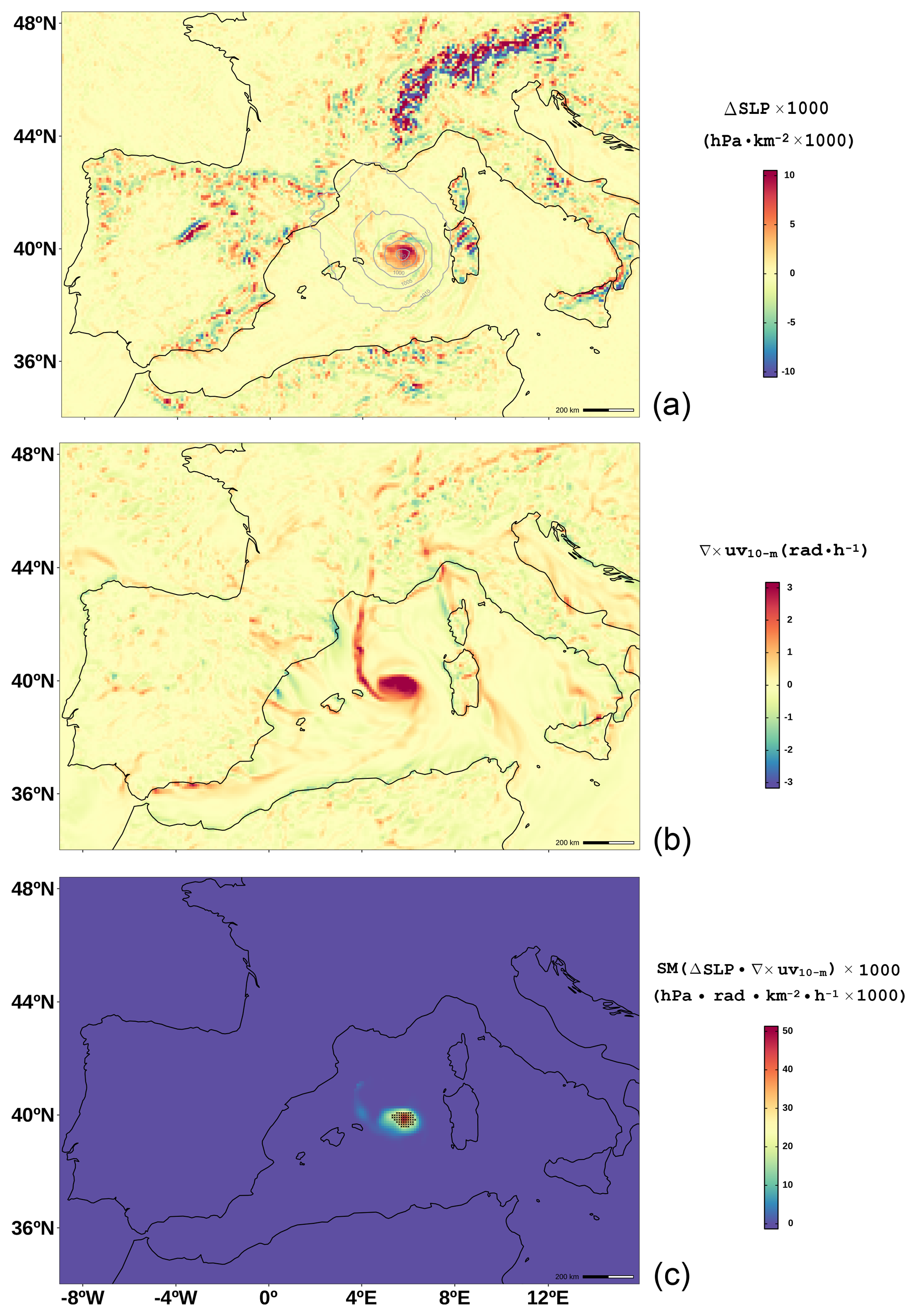
Figure 2 Three fields derived from the Rolf simulation with 9 km of grid spacing (see Appendix E). The SLP Laplacian is shown in colors along with SLP contours colored in grey (a); the 10 m wind curl and cyclonic potential C are presented in panels (b) and (c), respectively. Black crosses in (b) represent points selected as center candidates before checking the Hart conditions.

Once the cyclonic potential is calculated, the center candidates are selected by imposing the conditions described in Sect. 3.1.1 and 3.1.2 (the default values for all the parameters are used; see Appendix A). The points selected as center candidates (56) are represented in Fig. 2c with black crosses. Note that, given the intensity and well-defined symmetric shape of the medicane, all the points selected by the percentile are inside the medicane domain, and none are filtered out by the conditions. In this case, given the small domain extent, all the points are grouped within a single cluster. Finally, the centers inside the cluster are reordered by SLP value, and the Hart parameters are calculated until a center is found.

As discussed above, the medicane center selected does not necessarily coincide with the SLP minimum. This is particularly true when the SLP minimum does not satisfy the Hart conditions or any of the conditions imposed before. This is clearly illustrated in Fig. 3, where the bottom panel represents the fulfillment of the Hart conditions by the SLP minimum (not the absolute one but that inside the zero-vorticity domain, which is selected as the medicane center if it fulfills the Hart conditions) and the center selected by the algorithm. A filled circle indicates that the point meets the Hart conditions, and its color is related to the SLP value. The other symbols indicate the Hart condition imposed by the SLP minimum point when it does not coincide with the medicane center found by the algorithm. Top panels represent the Hart phase space plots for both sets of data. As expected, the algorithm classifies many more time steps as medicanes than those obtained by using only the SLP minimum. Furthermore, from the top panels we can conclude that, most of the time, it is the symmetry condition for the geopotential height thickness preventing the SLP minimum point from fulfilling the Hart conditions and hence from being selected as the medicane center.

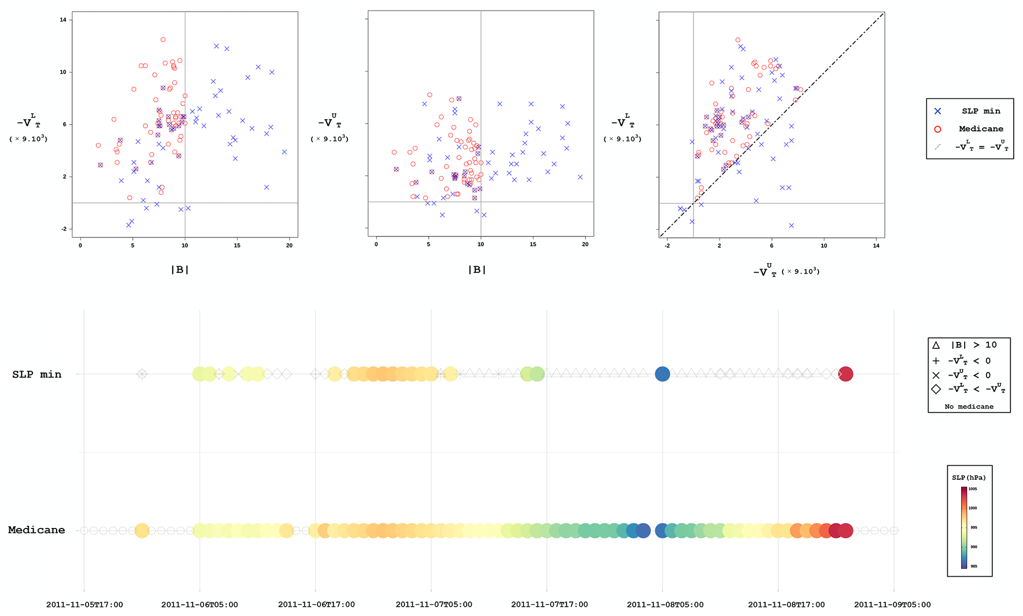
Figure 3 SLP minima and medicane centers for the Rolf medicane. In the top panels are the Hart phase space plots for points of SLP minimum (blue crosses) and centers detected by the algorithm (red circles). The bottom plot shows the temporal scheme of the detected centers and the SLP minimum track. Symbols indicate the Hart condition(s) not satisfied by the SLP minimum.

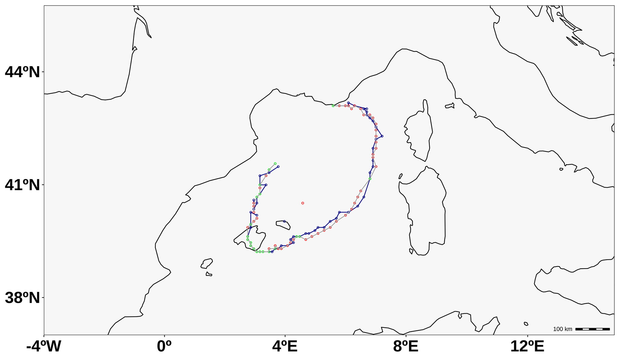
Figure 4 Rolf medicane tracks. The blue line represents the track calculated from the medicane centers found by the algorithm; the grey line is the one calculated with the SLP minimum. Green dots represent the points at which the SLP minimum fulfills the Hart conditions and is selected as the medicane center. The red dots represent the SLP minimum when there is no coincidence with the medicane center detected by the algorithm (blue points).

In addition, Fig. 4 shows the complete trajectory of the Rolf medicane as tracked by the algorithm presented here, along with the SLP relative minimum found at each time step in the proximity of the medicane center. This track is the result of passing the complete algorithm to the simulation with the default values of the parameters, as presented in Appendix A. When there is no coincidence between the SLP minimum and the found center for the medicane, marked in blue, it means that the SLP minimum does not fulfill the Hart conditions and is colored in red. Conversely, a green dot marks the SLP minimum for the time steps in which it fulfills the Hart conditions and is selected as the medicane center.

Therefore, we conclude that the center of the medicane does not coincide with the SLP minimum for the conditions imposed (see table in Appendix A for further detail) for a large portion of the time steps. Hence, tracking the SLP minimum and checking the Hart conditions after the tracking method would result in a loss of the medicane character for a majority of time steps. In this sense, the obtained tracking is almost point-by-point connected (a medicane is found in almost every time step) and thus more robust. This behavior can be attributed to the tilting of the medicane core. In Fig. 5, we compare the medicane structure for two different time steps. The structure is represented (panels a and c) by the cross section of the equivalent potential temperature θ_e (colors), the SLP (dashed grey line), and the geopotential height thickness (Z₆₀₀−Z₉₀₀) scaled to the zero–one interval (unity-based normalization). Figure 5b and d correspond to a spatial latitude–longitude projection of the SLP (colors) and the geopotential height 600–900 hPa layer thickness (dashed contours). In the first case, corresponding to 7 November 2011, 13:00 UTC (Fig. 5a, b), the relative SLP minimum among the points of the medicane activity area is within the highest (Z₆₀₀−Z₉₀₀) layer thickness isoline (right), which is the medicane center coincident with the point showing the lowest SLP value. In addition, the cross section reveals a perfect correspondence between the SLP minimum and layer thickness maximum, as well as great symmetry of θ_e around the vertical axis traced through the medicane center. This is related to a non-tilted medicane core.

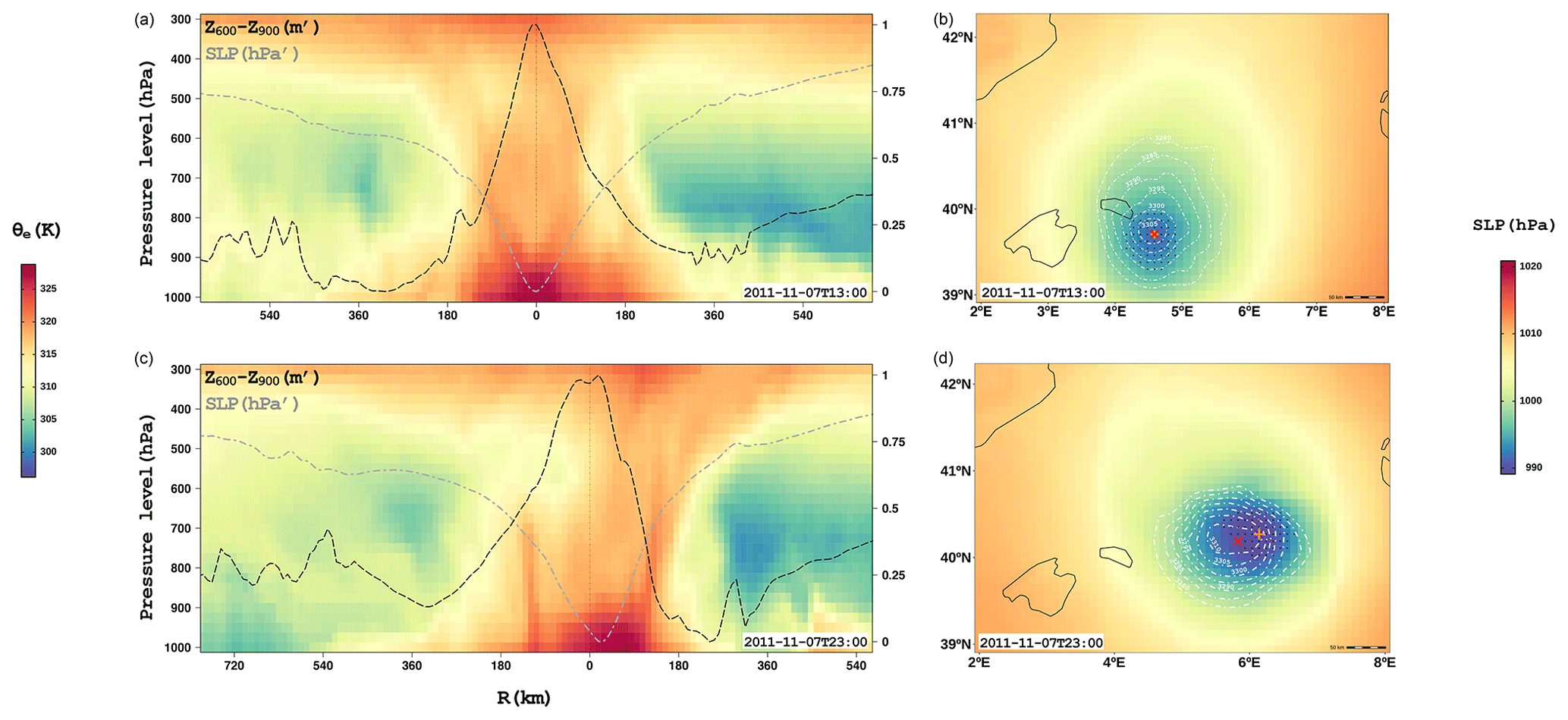
Figure 5 Depiction of the thermal structure of the Rolf medicane structure at two different time steps (a, b: 7 November 2011, 13:00 UTC; c, d: 7 November 2011, 23:00 UTC) by means of a zonal cross section (along the line of latitude passing through the medicane center found by the algorithm) of the equivalent potential temperature (colors in a, c) and a contour plot of Z₆₀₀−Z₉₀₀ along with the SLP field in colors (b, d). In (a, c), the SLP (black dotted curve) and Z₆₀₀−Z₉₀₀ (grey dotted curve) are also presented, both scaled to the zero–one interval (unity-based normalization). A vertical line indicates the longitudinal position of the center found by the algorithm. In (b) and (d), dashed white lines show contours of the geopotential height thickness for the 900–600 hPa layer every 5 m starting from 3280 m. Additionally, the orange plus symbol specifies the position of the SLP minimum, while the red cross denotes the position of the medicane center selected by the algorithm.

Conversely, in the second case, corresponding to 7 November 2011, 23:00 UTC (Fig. 5c, d), the medicane center detected by the algorithm is not coincident with the SLP minimum. The SLP minimum is almost out of the highest thickness contour and is 30 km away from the medicane center (about 30 % of the medicane radius). The value of the Hart B parameter for the medicane center (dotted black vertical line) is 9 m, while for the SLP minimum at the same latitude of the actual medicane center it is 20 m. Note that the medicane center is coincident with the maximum value of thickness. For this time step, the θ_e vertical pattern does not show symmetry around the axis but a tilting of the medicane core.

Therefore, the high capacity of our algorithm to detect medicanes is mainly based on the ability to recognize situations in which the medicane presents a slightly tilted structure. This tilting is not present in tropical cyclones and is what leads medicanes to easily lose their structure, thus encumbering the task of medicane tracking.

4.2 A deeper low in the domain

Considering the way the algorithm was conceived and developed, it should be able to isolate medicane structures even in the presence of a deeper low in the domain. In order to verify this ability, a simulation of the Rolf medicane is run with a domain extending to high latitudes, where the development of deep lows is very common. To reduce the computational cost of the simulation and to test the algorithm with fields of coarser grid spacings, this simulation is run at 27 km (see details in Appendix E).

Figure 6a shows the SLP field for the whole domain on 7 November 2011, 12:00 UTC. The synoptic situation is characterized by a deep extratropical cyclone located in the North Atlantic with a pressure center lower than 980 hPa. Simultaneously in the western Mediterranean Sea, a potential medicane (Rolf) appears with a pressure center around 1000 hPa. Figure 6b shows the cyclonic potential C for the same time step. In this first algorithm step we see how both cyclones are isolated, highlighting the medicane structure. High vorticity values are also present associated with the cold front in the Atlantic low. In the second step (Fig. 7a), the quantile filter (black crosses) and the vorticity threshold filter (red crosses) are applied. In the next step (Fig. 7b), the points with the required zero-vorticity radius symmetry are selected (blue crosses). Therefore, at this point we have two clusters with several medicane center candidates, whose representative points (highest C value points) are represented as large red plus symbols (one for the Atlantic low and one for the Mediterranean low) in Fig. 7b.

Figure 6 SLP (a) and scaled smoothed cyclonic potential C C (b) for the Rolf simulation at 27 km of grid spacing. for both fields corresponds to 7 November 2011, 12:00 UTC.

Figure 7 Scaled smoothed cyclonic potential C for the Rolf simulation at 27 km of grid spacing on 7 November 2011, 12:00 UTC, along with the points selected by the algorithm as potential medicane center candidates. (a) Candidates after the quantile filter (black crosses) and after the vorticity threshold filter (red crosses). (b) Candidates after the symmetry filter (blue crosses), cluster representative points (red plus symbols), and medicane center selected by the algorithm (green plus symbol).

Finally, the algorithm results for this time step show how there is no point fulfilling the Hart conditions in the Atlantic low, while it correctly finds a medicane center in the Mediterranean low (green plus in Fig. 7b). Therefore, the algorithm successfully achieves the desired isolation of the medicane despite the presence of a deeper low within the domain. The final track obtained is presented in Fig. 8 (blue line). The domain is cropped to the western Mediterranean area given that no medicane center is found by the algorithm for the Atlantic low. In addition, the ability of the algorithm to assimilate and handle several sources of data is also illustrated. The track of the medicane from the ERA5 reanalysis as calculated by the algorithm over a similar spatial domain is also presented (Fig. 8, dark red line).

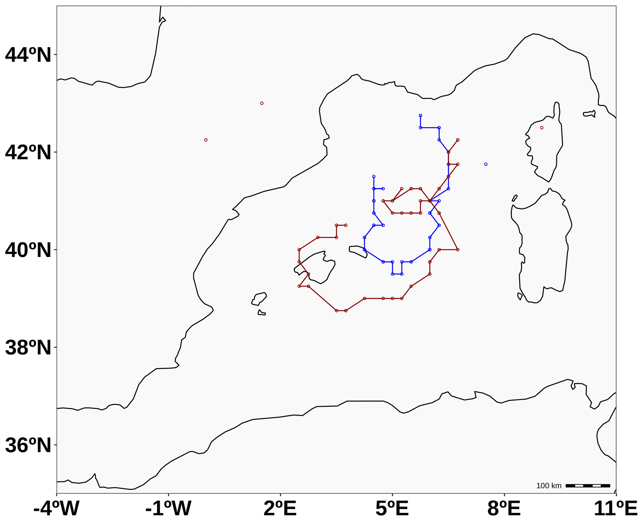
Figure 8 Rolf medicane tracking from the WRF simulation at 27 km (blue track) and from ERA5 reanalysis data (dark red track) at 0.25^∘ of grid spacing cropped to the western Mediterranean area (see green box in Fig. E1). ERA5 data are used in hourly resolution in order to get a precise track. The values of the algorithm parameters for these two simulations are the default ones, as indicated in Appendix A. However, for the B threshold, B_threshold=20 m is used instead of 10 m provided that ERA5 shows a less intense medicane than the numerical simulations performed with the WRF model, and thus the medicane structure is not so well defined, leading to a higher asymmetry. Changing the B parameter in the algorithm for the detection of medicanes in reanalysis data serves as a test for the algorithm flexibility and sensitivity to the different namelist parameters.

4.3 Medicane independence from the low pressure center

As previously stated, an important drawback of algorithms based on the search for new track points depending on previous ones lies in its strong dependence on the selection of the first time step, regardless of the criteria used to confine the search area for the subsequent point.

To illustrate this problematic situation, we select a 9 km WRF simulation of the Celeno medicane (see Appendix E for details). The simulation reproduces the generation of the medicane. Although the obtained track does not fit the one reported by former studies (Pytharoulis et al., 1999; Lagouvardos et al., 1999), this simulation still seems valid for testing the algorithm.

The meteorological situation is characterized by an eastward-moving extratropical cyclone (see Fig. 9) detected on 13 January 1995 at 08:00 UTC and traveling until 14 January 1995 at 09:00 UTC as far as the north of the Libyan coast. During the morning of 14 January 1995 a strong cyclogenetic character appears within an area around the Ionian Sea (see Fig. 9), emerging as a medicane on 14 January 1995 at 14:00 UTC that travels first to the west and then turns to the southeast. Finally, the medicane reverses into an extratropical cyclone traveling throughout the eastern Mediterranean Sea.

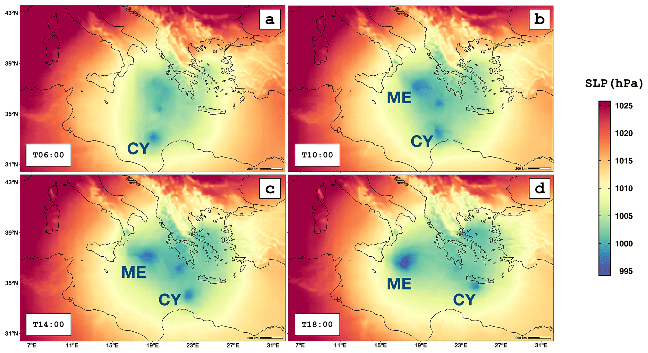
Figure 9 SLP field on 14 January 1995 at 06:00 UTC (a), 10:00 UTC (b), 14:00 UTC (c), and 18:00 UTC (d). The SLP minimum of the extratropical cyclone center is labeled CY, while the medicane is marked with the ME label.

Therefore, the model reproduces a situation in which two main lows coexist in the domain for a few hours (Fig. 9). Using a time-dependent algorithm, if it started tracking in the time step shown in panel (a), the initial point would correspond to the minimum SLP (labeled CY). Tracking this point would lead to following one low that will not satisfy the warm-core conditions of being the medicane (with the ME label) located 400 km away from the actual cyclone (panel d). Then, while the former is more intense in terms of SLP minimum, it is the latter one that fulfills the conditions of being a medicane. The algorithm does not follow the synoptic low (CY) since it does not satisfy other conditions such as symmetry (Fig. 10).

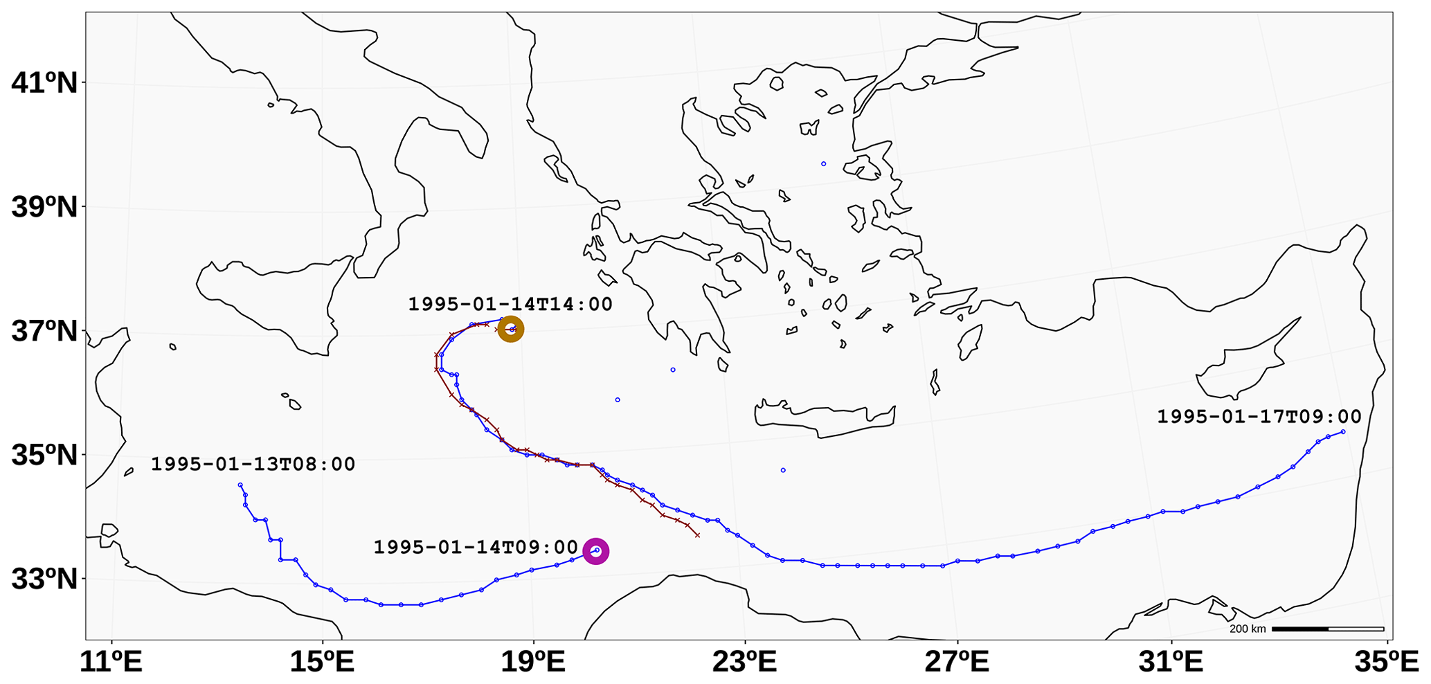
Figure 10 Tracks of cyclones between 12 and 18 January 1995. The dark red line corresponds to the medicane track, and blue lines represent the tracks calculated excluding the Hart condition check in the algorithm namelist. Thus, the blue lines are the complete cyclone tracks during their entire lifetime, while the dark red line is the track of the cyclone when the conditions for being a medicane are fulfilled. The purple circle represents the last point at which an existing low-pressure center fulfills the filters (except the Hart conditions), while the gold one is the first location of another cyclone, which appears 5 h after the extinction of the previous one and ends having a medicane structure (dark red line). The synoptic low (labeled CY in Fig. 9) is not tracked from 14 January 1995, 09:00 UTC, forward since it does not satisfy the symmetry condition, among others.

This example shows how a time-independent method provides the algorithm with the capability to track several lows, which in certain circumstances is necessary to permit a correct detection of the medicane.

4.4 Coexistence of two simultaneous medicanes

One remarkable feature of this algorithm is its ability to capture several simultaneous warm-core structures. In this section we present the application of the algorithm to a 9 km WRF simulation of the Leucosia medicane event. The simulation period was 19–28 January 1982. More details about the experiment can be found in Appendix E. Although there is no evidence that this event showed two simultaneous medicanes (Ernst and Matson, 1983; Reed et al., 2001), the simulation reproduces them. Therefore, it serves as a particularly interesting trial for the algorithm, given that the algorithm implementation allows the parameter tuning to search for other types of cyclones more likely to coexist in the same domain.

The simulation reproduces the formation of two coexisting medicanes during a period of 24 h. Figure 11 presents the tracks detected by the algorithm for the whole simulated period and the SLP field for a time when both warm-core structures coexist. The track located at the north of Libya corresponds to the documented tropical-like cyclone event Leucosia, which maintained its medicane characteristics from early 25 to mid-26 January. Another tropical-like cyclone coexisted with Leucosia for 24 h starting on 25 January 1982, 04:00 UTC, and faded after reaching the Apulia region of the Italian Peninsula.

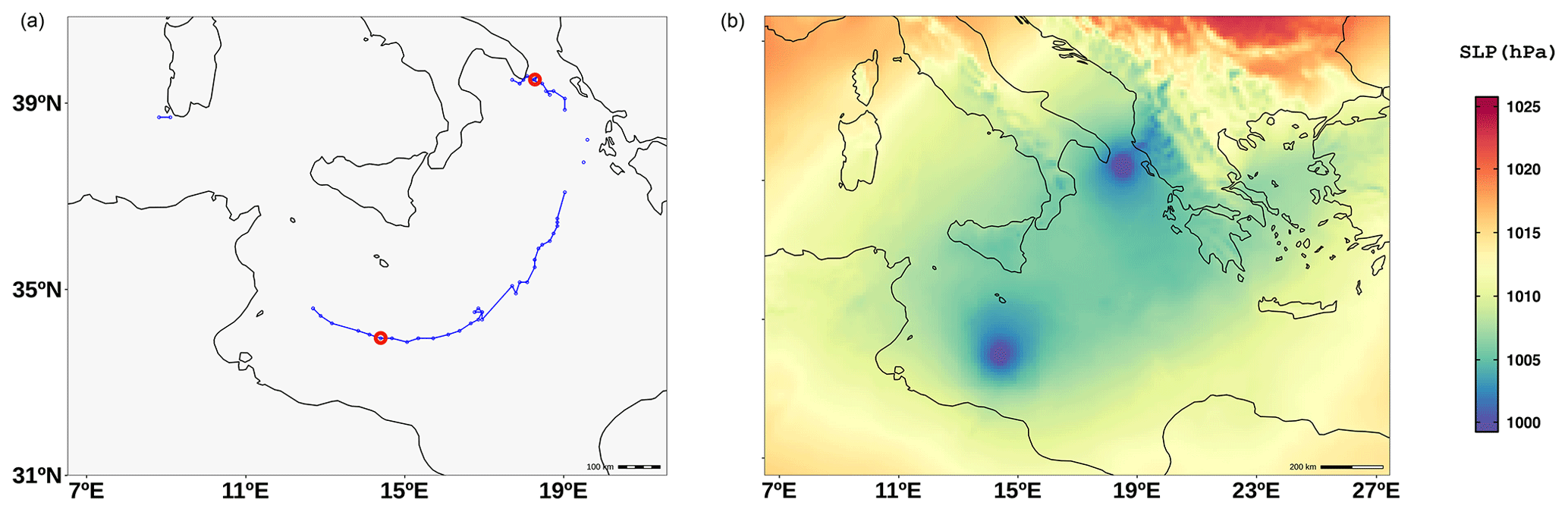
Figure 11 Tracks and SLP field for the Leucosia medicane simulation. Blue circles represent the medicane centers found in successive time steps (a). The two red circles correspond to the location of the two medicanes on 25 January 1982, 12:00 UTC. Panel (b) shows the SLP (hPa) for that time.

While this situation may not seem likely, the interesting point here is that the algorithm is prepared to avoid the Hart conditions and track regular cyclones. Since, unlike two medicanes, the coexistence of two cyclones in general is a very common event, we remark here on the ability of the algorithm to track simultaneous storms.

5 Conclusions

In this work, a new algorithm specifically suited for medicane tracking has been presented. The algorithm is robust and capable of detecting and tracking them even in adverse conditions, such as the existence of larger or more intense systems within the domain, the coexistence of multiple tropical-like systems, or the existence of complex orographic effects. This algorithm implements a time-independent methodology whose search methodology does not rely on previous time steps, hence the time independence. Although it is especially suited for medicanes, it also provides the possibility of an easy modification of the cyclone definition parameters to make it useful for the detection of different cyclone types.

The algorithm is mainly based on a cyclonic potential field C, and the method applies successive filters over all grid points on each time stamp, leading to a final list of center candidates. After grouping them to allow the existence of multiple cyclones in the same domain, the Hart conditions are used to select a single center within each cluster of candidates, i.e., for each medicane structure. Eventually, the found centers are connected over time and space, and a complete medicane track is obtained as the main product of the algorithm. The computational efficiency and time-saving performance have been key factors taken into account for the development of this algorithm. Consequently, it should be suitable for further medicane climatological studies.

The selected examples showcase how the algorithm presented throughout this paper is useful and robust for the tracking of medicanes. The tracking algorithm allows for the detection of these storms even in the weakest phases of the weakest events, differentiating this type of storm from midlatitude cyclones. This methodology satisfies the requirements expected for a tracking method of this nature, namely the capacity to track multiple simultaneous cyclones, the ability to track a medicane in the presence of an intense trough inside the domain, the potential to separate the medicane from other similar structures by handling the intermittent loss of structure, and the capability to isolate and follow the medicane center regardless of other cyclones that could be present in the domain.

The use of TITAM for the automated detection of other types of cyclones, or even for the detection of medicanes at early or late stages, can be easily achieved by modifying the Hart condition module within the algorithm namelist. When ignoring the Hart conditions, the selected center represents the point with the lowest SLP value among the points with the highest C value fulfilling the zero-vorticity radius symmetry condition. This is virtually equivalent to tracking the SLP minimum along its motion, as long as it fulfills the zero-vorticity radius symmetry condition. Despite its complexity due to the existence of multiple parameters, the namelist-oriented implementation provides it with the flexibility needed to apply it to the tracking of other kinds of cyclones. Thus, it is an extensible tool that can be used for the automated identification of medicanes and other types of cyclones (tropical and extratropical) in large datasets such as in regional climate change experiments. The complete TITAM package is available as free software extensively documented and prepared for its deployment (see “Code availability”).

As a final remark, this algorithm sheds some light on medicane understanding regarding medicane structure, warm-core nature, and the existence of tilting.

Appendix A: Algorithm parameter description and default values

Parameter	Definition	Default value
InitTime	Initial time step for the medicane search. No medicanes will be found for time stamps before this one. If the string “initial” is used, the first time stamp in the input file will be used as the initial time step.	initial
FinalTime	Final time step for the medicane search. No medicanes will be found for time stamps after this one. If the string “final” is used, the last time stamp in the input file will be used as the initial time step.	final
Resolution	Spatial horizontal grid spacing of the NetCDF (km). Resolution is assumed to be the same in both directions. Future versions of the algorithm will support different grid spacings for both longitudinal and latitudinal dimensions for large grids in non-regular projections. It has no default value, so the string RR is used and, if not changed, will generate an error, as it is expecting a number.	RR
TimestepDt	Temporal resolution of the NetCDF (in hours). The default value is 1 h between NetCDF time stamps.	1 h
LonDimName	Name of the longitude dimension in the NetCDF. It takes the name west_east for wrf-python output and “lon” for ERA5 and ERA-Interim reanalysis data.	west_east
LonVarName	Name of the longitude variable in the NetCDF. It takes the name XLONG for wrf-python output and “lon” for ERA5 and ERA-Interim reanalysis data.	XLONG
LatDimName	Name of the latitude dimension in the NetCDF. It takes the name south_north for wrf-python output, and “lat” for ERA5 and ERA-Interim reanalysis data.	south_north
LatVarName	Name of the latitude variable in the NetCDF. It takes the name XLAT for wrf-python output and “lat” for ERA5 and ERA-Interim reanalysis data.	XLAT
TimeDimName	Name of the time dimension in the NetCDF. It takes the name “Time” for wrf-python output and “time” for ERA5 and ERA-Interim reanalysis data.	Time
PressureVertLevelDimName	Name of the vertical level dimension for 3D variables in the NetCDF. It takes the name interp_level for wrf-python output and “plev” for ERA5 and ERA-Interim reanalysis data.	interp_level
SLPVarName	Name of the SLP variable in the outputfile-slp.nc NetCDF. It takes the name “slp” for wrf-python output and “var151” for ERA5 and ERA-Interim reanalysis data.	slp
U10VarName	Name of the 10 m wind U variable in the outputfile-uvmet10-U.nc NetCDF. It takes the name “uvmet10” for wrf-python output and “var165” for ERA5 and ERA-Interim reanalysis data.	uvmet10
V10VarName	Name of the 10 m wind V variable in the outputfile-uvmet10-V.nc NetCDF. It takes the name “uvmet10” for wrf-python output and “var166” for ERA5 and ERA-Interim reanalysis data.	uvmet10

Parameter	Definition	Default value
ZVarName	Name of the geopotential height variable in the outputfile-z.nc NetCDF. It takes the name “height” for wrf-python output and “var129” for ERA5 and ERA-Interim reanalysis data.	height
SmoothingPasses	Number of passes of the 1–2–1 smoothing of the product field. This product is the result of a pointwise multiplication of the SLP Laplacian and the 10 m wind rotational (vorticity at 10 m – surface level). The number of passes is the number of times that smoothing is sequentially performed. The default value is 5; a value above 3 is recommended.	5
SLPThreshold	Threshold for the first filter. It is an SLP minimum value, which should be fulfilled by every point being a center candidate. Defaults to 1005 hPa, which is expected to be exceeded on a medicane center.	1005 hPa
ProductQuantileLowerLimit	Parameter of the second filter. It represents the quantile lower limit applied to the product field, above which all points are selected as center candidates. This is not a necessary filter from a physical view, but it is a critical one for computational reasons. If not applied, we would have to calculate the Hart parameters for each grid point, which is highly expensive. Defaults to 0.999 (99.9 percentile). This means that, in a 200×200 grid, only 40 points are selected as center candidates.	0.999
VorticityThreshold	Threshold for the third filter. It is a vorticity minimum value, which should be exceeded by every point being a center candidate. This filter is applied to the center candidates selected by the above quantile and performs as an efficiency filter, avoiding the calculation of the Hart parameters in conditions with a lack of vorticity in the domain, which is related to the absence of cyclonic activity. Defaults to 1 rad h−1, a number obtained by means of our own ad hoc numerical study of typical vorticity values in the presence or absence of medicanes.	1 rad h−1
CalculateZeroVortRadiusThreshold	Measure to calculate the variable radius, which will be used in the calculation of Z-gradient symmetry and Hart parameters. The options are “zero” and “mean”. If zero is chosen, the radius is calculated as the mean radial distance from the center to the zero-vorticity line. If mean is chosen, it is the distance to the contour of the vorticity mean domain value. Defaults to zero.	zero
CalculateZeroVortRadiusDistance	The length of the lines along which the vorticity sign changes (if the threshold is zero) or the mean value (if the threshold is the mean) is searched in eight directions. Determines the maximum size of the structures allowed in the domain, since if no critical point (zero or mean vorticity) is found on any of the directions, the point is discarded. Defaults to 300 km.	300 km

Parameter	Definition	Default value
IfCheckZeroVortSymm	Whether to apply the zero-vorticity symmetry filter based on asking the contour of zero-vorticity around the center candidate to be axisymmetric. It is calculated by taking eight directions and getting the distance at which the vorticity changes its sign. If this sign change is not reached in the number of points requested (see previous parameter), then it is set to Inf – 1e10 –. This filter is dependent on the fact that tropical cyclones, and therefore medicanes, must have a closed circulation. Defaults to TRUE.	TRUE
ZeroVortRadiusMaxAllowedAsymm	Maximum asymmetry (km) allowed for the zero-vorticity radius calculation. This means that a center candidate is discarded if the difference between any pair of the eight calculated distances is higher than this allowed asymmetry value. The lower this parameter value, the more restrictive the symmetry condition imposed. Defaults to 300 km.	300 km
ZeroVortRadiusMinSymmDirs	Minimum number of directions (out of eight) that should be “non Inf”. In other words, the minimum number of directions in which a sign change should be found within the distance specified in the previous parameter. The higher the number of directions, the more symmetry is requested. This prevents the method from failing in cases of spiraling vorticity fields, for which a large enough spiral arm matching the calculation direction could lead to constant signed vorticity values. Defaults to six directions (out of eight).	6
ZeroVortRadiusUpperLimit	Upper limit for the zero-vorticity radius. If a center candidate is calculated with a zero-vorticity radius above this upper limit, it is discarded as a medicane center candidate. Medicane outer radius typical values are between 100 and 300 km. A nonrestrictive default value of 1000 km is used.	1000 km
ZeroVortRadiusLowerLimit	Lower limit for the zero-vorticity radius. If a center candidate is calculated with a zero-vorticity radius below this lower limit, it is discarded as a medicane center candidate. Medicane outer radius typical values are between 100 and 300 km. Default value is 80 km.	80 km
SLPminsClustersMinIBdistance	The minimum distance between two points to be considered to belong to different clusters and thus to be candidates for two different medicane centers. This parameter should be directly related to the mean size of the cyclone for which we are searching. Default value is 300 km, given that medicanes are usually between 100 and 200 km in radius.	300 km

Parameter	Definition	Default value
MaxNumberOfDifferentClusters	Maximum number of different cyclones that can be found in the analyzed domain at a given time step (i.e., the maximum allowed number of concurrent cyclones). If all restrictions are removed, the filters are ignored, and the Hart conditions not checked, we would be searching for cyclones, and in domains that are large enough, a huge number of cyclones could appear. This is the motivation for the inclusion of this parameter. In the case of exceedance, the centers that will be found are the ones with higher product value, which means those with a greater cyclonic nature. Defaults to 50, a limit that is high enough when looking for medicanes and using all the filters, but it could be surpassed for certain combinations of these parameters.	50
MinPointsNumberInCluster	Filter to remove center candidates. Once the center candidates are split into clusters that are farther than a certain distance from any other cluster, all the groups that contain fewer than a certain number of points are discarded. This number represents the minimum number of points that a group must have to be considered a potential cyclone center. This is a filter oriented to remove orographic artifacts that, given their singular placement, can have high wind curl values and a positive value of the Laplacian (interpolation effects may lead to artifacts in the SLP surface, showing low values in orographic systems). However, these critical points are usually isolated and hence removed with this filtering. Defaults to five points inside the cluster. Its value should be consistent with the number of points selected by the quantile filter.	5
IfCheckHartParamsConditions	The Hart parameters are three parameters stated by Hart in 2003 conceived to define the tropical nature of a cyclone in an objective manner. He defined a parameter B, directly related to the thermal symmetry of the cyclone, and two parameters of thermal wind in the lower and upper troposphere, showing a deep connection with the warm-core nature of the system. From these three parameters, four conditions should be fulfilled by a tropical cyclone. Default value is TRUE and then Hart conditions are checked.	TRUE
HartConditionsTocheck	The Hart conditions are (1) B<Bthreshold – m – (see parameter Bthreshold); (2) $-V_{\mathrm{T}}^{\mathrm{L}}>\mathrm{0}$; (3) $-V_{\mathrm{T}}^{\mathrm{U}}>\mathrm{0}$; (4) $-V_{\mathrm{T}}^{\mathrm{L}}>-V_{\mathrm{T}}^{\mathrm{U}}$. If Hart conditions are checked, i.e., if the previous parameter is set to TRUE, any condition can be removed and will not necessarily be TRUE for a point to be considered a medicane. Defaults to $\mathrm{1},\mathrm{2},\mathrm{3}$, and 4, and all the conditions are checked.	$\mathrm{1},\mathrm{2},\mathrm{3},\mathrm{4}$
Blowerpressurelevel	Lower pressure level for the calculation of the B parameter (Hart, 2003). Defaults to 900 hPa.	900 hPa
Bupperpressurelevel	Upper pressure level for the calculation of the B parameter. Defaults to 600 hPa.	600 hPa
Bmultiplemeasure	If multiple directions are used to calculate a more constrained B parameter, this is the measure to use. Defaults to “max”.	max

Parameter	Definition	Default value
Bdirections	Number of directions to be used in the calculation of the more restrictive B parameter. The maximum allowed is four directions, and at least two directions are recommended. Defaults to four directions.	4
Bthreshold	Threshold – in meters – of the thermal symmetry parameter B. It represents the maximum allowed thermal asymmetry in the thickness of the geopotential height layer between the left and the right side of a circle centered in the point checked divided by a vector in the direction of motion of the cyclone. Hart recommends a value of 10 m for tropical cyclones. Although this may be too strong of a limitation for medicanes, whose symmetry is not as well defined as in the former ones, a default value of 10 m is used for the threshold of B.	10 m
LTWlowerpressurelevel	Lower pressure level for the calculation of the $V_{\mathrm{T}}^{\mathrm{L}}$ (lower tropospheric thermal wind) parameter. Defaults to 900 hPa.	900 hPa
LTWupperpressurelevel	Upper pressure level for the calculation of the $V_{\mathrm{T}}^{\mathrm{L}}$ (lower tropospheric thermal wind) parameter. Defaults to 600 hPa.	600 hPa
UTWlowerpressurelevel	Lower pressure level for the calculation of the $V_{\mathrm{T}}^{\mathrm{U}}$ (upper tropospheric thermal wind) parameter. Defaults to 600 hPa.	600 hPa
UTWupperpressurelevel	Upper pressure level for the calculation of the $V_{\mathrm{T}}^{\mathrm{U}}$ (upper tropospheric thermal wind) parameter. Defaults to 300 hPa.	300 hPa

Appendix B: Algorithm input specifications

As mentioned in Sect. 2, the input data for the algorithm described in this paper consist of multiple NetCDF (.nc) files containing temporal series of certain meteorological fields. The mandatory 2D and 3D fields are sea level pressure (SLP), 10 m wind horizontal components (U10, V10), and geopotential height (Z) for at least the 900, 800, 700, 600, 500, 400, and 300 hPa levels. Note that the more vertical levels there are, the more precise the Hart thermal wind parameter calculation will be (a minimum of 20 vertical levels is recommended for obtaining trustworthy results). The requested units for the fields are hectopascals (hPa) for SLP, meters for geopotential height, and kilometers per hour (km h⁻¹) for both 10 m wind horizontal components.

If a WRF output file is to be used as input data for the algorithm, then the use of the provided pinterpy package is strongly recommended (https://doi.org/10.5281/zenodo.3874416, Pravia-Sarabia et al., 2020). In the namelist file interp-namelist, the input file name must be changed to the WRF output file containing all the time steps (the ncrcat command for NetCDF Operators (NCO) tools is referred to for the task of temporal merging). Detailed instructions on the requested Python version and libraries for a successful running can be found in the README.md file (https://doi.org/10.5281/zenodo.3874416, Pravia-Sarabia et al., 2020), while specific pinterpy usage instructions and a detailed description of the namelist parameters can be found in the README.interp-namelist file inside the pinterpy package (https://doi.org/ 10.5281/zenodo.3874416, Pravia-Sarabia et al., 2020).

In the case of using input data different from WRF output, the metadata must be closely inspected and the following parameters must be set accordingly in the FindMedicanes.namelist file: LonDimName, LonVarName, LatDimName, LatVarName, TimeDimName, PressureVertLevelDimName, SLPVarName, U10VarName, V10VarName, and ZVarName. The vertical levels in the geopotential height 3D field do not need to follow a specific order, and both increasing and decreasing sortings are allowed and automatically detected.

Appendix C: Technical notes on the algorithm deployment and multicore performance

The algorithm execution requires prior installation of the R environment with the “ncdf4” and “oce” libraries. Details on the recommended R version and the oce library installation process can be found in the README.md file (https://doi.org/10.5281/zenodo.3874416, Pravia-Sarabia et al., 2020).

As mentioned in Sects. 1 and 3, multicore parallel computing is supported and encouraged. The libraries for each and doParallel are requested for this type of execution. If these libraries are not installed or will not be required (single core run), the flag for the number of cores, 1, needs to be used as a second argument when running the algorithm, with the first argument being the input file or folder. See further details in the README.md file (https://doi.org/10.5281/zenodo.3874416, Pravia-Sarabia et al., 2020).

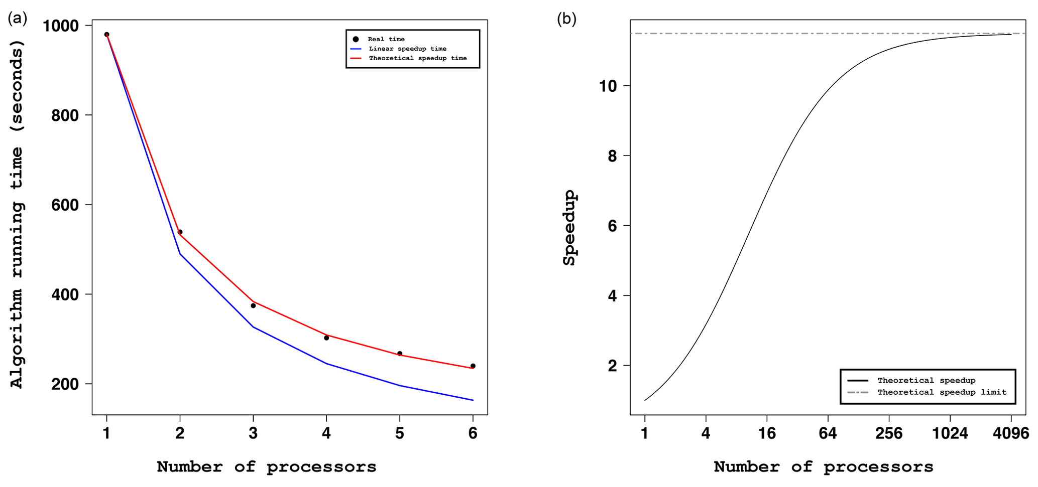
Figure C1 Parallel performance of the tracking algorithm. (a) The experimental execution times of the algorithm (black dots) as a function of the number of processors for the parallel computing. The red curve represents the fit of Amdahl's law to the data (P=0.087); in blue is the “linear speedup” theoretical curve (P=0). (b) The adjusted Amdahl's law curve (P=0.087) versus the number of processors (solid black line), asymptotically reaching 𝒮=11.5 (dashed grey line).

Regarding the parallelization implemented in the algorithm, we test its performance by means of different algorithm executions over the Rolf simulation with 27 km of grid spacing (described in Appendix E and analyzed in Sect. 4.2). Figure C1a shows the execution times for the different runs of the algorithm, changing the number of processors for the calculation (black dots).

In computer science, Amdahl's law (Amdahl, 1967) defines the speedup achieved when increasing the number of processors that compute in parallel as a function of the proportion of the code that must be processed serially (P). It is often expressed as

$$\begin{array}{}\text{(C1)}& \mathcal{S}={\displaystyle \frac{\mathrm{1}}{P+\frac{\mathrm{1}-P}{N}}},\end{array}$$

where 𝒮 is the speedup, P the nonparallelizable proportion of code, and N the number of processors. In the particular case of a fully parallelizable code (P=0), there is a “linear speedup” when increasing the number of processors (blue line in Fig. C1a). In this same plot, an adjustment of a theoretical curve (red line) following Amdahl's law to our execution times (black dots) shows that for the particular case of the Rolf simulation at 27 km, P=0.087, which means that 91.5 % of the code is run in parallel. Figure C1b shows the theoretical speedup curve obeying Amdahl's law for P=0.087 with an increasing number of processors, reaching an asymptote at $\mathcal{S}=\mathrm{1}/\mathrm{0.087}\simeq \mathrm{11.5}$ for N→∞.

Appendix D: Post-processing tools included in the package

An additional tool is provided to extract further information on the medicane size and intensity. Provided with the RData file, which is the output of the medicane tracking algorithm, the getmedicanestrackdata bash script diagnoses additional variables from the found medicane centers. In the “reduced” mode, only longitude, latitude, and the SLP value of the medicane center are calculated. The “complete” method extends to other variables, such as the minimum SLP value inside the zero-vorticity radius, its position, and the 10 m maximum wind speed inside the medicane domain, which allows for the classification of the medicane category in terms of its intensity as defined on the Saffir–Simpson scale. Detailed information about this post-processing tool can be found in the README.md file (https://doi.org/10.5281/zenodo.3874416, Pravia-Sarabia et al., 2020).

Moreover, in Sect. 3.4 we defined the rules to connect two found medicane centers. Once the isolated points are connected, our next step is to create a plot with the calculated medicane track. To this end, an auxiliary plotting script is provided; see the README.md file for detailed instructions on its usage (https://doi.org/10.5281/zenodo.3874416, Pravia-Sarabia et al., 2020). Based on the more generic plotting function MatrixPlot.R (https://doi.org/10.5281/zenodo.3874416, Pravia-Sarabia et al., 2020), the plotmedicanestrack bash script produces a pdf receiving an RData file (output of the tracking algorithm) and the NetCDF files as input data.

It is also important to highlight that the function to plot the calculated medicane tracking expects either a regular grid in long–lat projection or an irregular one in a Lambert projection. Please note that this post-processing tool is not prepared to receive input data expressed in any other projection, although the tracking algorithm will run successfully. If the input data are neither WRF output nor long–lat projected data, lines 49 to 62 of the PlotTrack.R file (https://doi.org/10.5281/zenodo.3874416, Pravia-Sarabia et al., 2020) must be commented out and the CRS (Coordinate Reference System) must be set in proj4string notation according to the projection of the data in order to get an output map properly projected.

Appendix E: Review of the utilized WRF simulations

Given the relatively small horizontal extent of medicanes, fine grid spacing fields are needed to correctly interpret their thermal properties and dynamics. To achieve this high resolution, dynamical downscaling is often employed by means of so-called RCMs (regional climate models). For this study we produce the necessary meteorological fields for initial and boundary conditions by downscaling the ERA-Interim reanalysis with the WRF model (Skamarock et al., 2008). This model is highly sensitive to the domain configuration and set of parameterizations that determine how the dynamics as well as the physical and chemical mechanisms (in the case of the WRF-Chem coupled model) are solved. However, given that this work focuses on the algorithm rather than on the ability of the model to accurately reproduce medicane characteristics, we have kept the model configuration fixed to one that is physically consistent with the medicane main features and fostering processes.

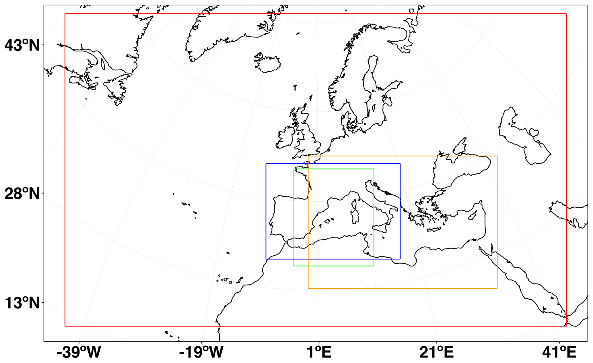
Figure E1 Spatial domains covered by the WRF simulations described above. Domains correspond to the following simulations: Rolf at 27 km (red), Rolf at 9 km (blue), and Celeno and Leucosia at 9 km (orange). Additionally, the green box covers the spatial area selected to run the algorithm on ERA5 data.

No physics suite (WRF preconfiguration of a set of well-tested physics parameterizations as a suite) is used for the model run. The chosen parameterizations lead to the following physical configurations of the model: the Morrison et al. (2009) second-moment microphysical scheme is used (mp_physics=10), and prognostic cloud droplet number is included in the Morrison microphysics scheme (progn=1). Radiation is parameterized with the Rapid Radiative Transfer Model for GCMs (RRTMG) by Mlawer et al. (1997) for both shortwave and longwave radiation, solved every 30 min. Additionally, the selected option for the surface layer parameterization is solved with the MM5 scheme based on the similarity theory by Monin and Obukhov (1954), while the Unified NOAH LSM option is used for the land surface calculation (Mitchell, 2005). The number of soil layers in land surface model is thus four. The Yonsei University scheme is employed for the boundary layer (Hong et al., 2006), solved every time step (bldt=0). For the cumulus physics, the Grell 3D ensemble (cu_physics=5; cudt=0) is chosen to parameterize convection (Grell and Dévényi, 2002). Heat and moisture fluxes from the surface are activated (isfflx=1), as is the cloud effect to the optical depth in radiation (icloud=1). Conversely, snow-cover effects are deactivated (ifsnow=0). Land use and soil category data come from WPS∕geogrid but with dominant categories recomputed (surface_input_source=1). Un urban canopy model is not considered (sf_urban_physics=0), and the topographic surface wind correction from Jiménez and Dudhia (2012) is turned on. Both feedback from the parameterized convection to the radiation schemes and SST update (every 6 h, coinciding with boundary condition updates) are also turned on.

As explained throughout the text, we have selected a number of historical events that cover a range of structures which serve as a test bed for the description and evaluation of the tracking algorithm. In particular, four different events have been simulated for the sake of the algorithm testing.

• First is the simulation of the Rolf medicane with 9 km of grid spacing. This event spans the period from 5 to 10 November 2011 with hourly resolution. This 9 km inner domain (blue bounding box in Fig. E1) is nested to a larger domain, which includes the Iberian Peninsula, Balearic Islands, and the territory of Italy with a coarser grid spacing of 27 km. The large domain is run with spectral nudging to ERA-Interim global data for wavelengths above 1000 km.

• Second is the simulation of the Rolf medicane with 27 km of grid spacing and hourly temporal resolution. Like the previous case, it includes the time range from 5 to 10 November 2011. A single large domain of 27 km is included, which covers the eastern Atlantic and Mediterranean areas, as well as latitudes from the north of Africa to Greenland (red bounding box in Fig. E1). This domain is also run with spectral nudging to ERA-Interim global data for wavelengths above 1000 km.

• Third is the simulation of the Celeno medicane between 12 and 18 January 1995 run with 9 km of grid spacing and hourly temporal resolution. This simulation is based on a first large domain of 27 km including all the Mediterranean basin with a nested domain of 9 km covering the eastern Mediterranean area (orange bounding box in Fig. E1). The coarser-resolution domain is run with spectral nudging to ERA-Interim global data for wavelengths above 1000 km.

• Fourth is the simulation of the Leucosia medicane from 19 to 28 January 1982 with hourly resolution in a small domain with 9 km of grid spacing (orange bounding box in Fig. E1) nested to a larger 27 km domain limited to the Mediterranean area. The large domain is run with spectral nudging to ERA-Interim global data for wavelengths above 1000 km.