New strategies for vertical transport in chemistry transport models: application to the case of the Mount Etna eruption on 18 March 2012 with CHIMERE v2017r4

Excessive numerical diffusion is one of the major limitations in the representation of long-range transport by chemistry transport models. In the present study, we focus on excessive diffusion in the vertical direction, which has been shown to be a major issue, and we explore three possible ways of addressing this problem: increasing the vertical resolution, using an advection scheme with anti-diffusive properties and more accurately representing the vertical wind. This study was carried out using the CHIMERE chemistry transport model for the 18 March 2012 eruption of Mount Etna, which released about 3 kt of sulfur dioxide into the atmosphere in a plume that was observed by satellite instruments (the Infrared Atmospheric Sounding Interferometer instrument, IASI, and the Ozone Monitoring Instrument, OMI) for several days. The change from the classical Van Leer (1977) scheme to the Després and Lagoutière (1999) anti-diffusive scheme in the vertical direction was shown to provide the largest improvement to model outputs in terms of preserving the thin plume emitted by the volcano. To a lesser extent, the improved representation of the vertical wind field was also shown to reduce plume dispersion. Both of these changes helped to reduce vertical diffusion in the model as much as a brute-force approach (increasing vertical resolution).

1 Introduction

Among many other uses, such as the operational forecast of air quality, chemistry transport models (CTMs) have been used successfully in the past to represent the long-range transport of polluted plumes from different types of sources (e.g., mineral dust, volcanic eruptions and biomass burning). The CHIMERE¹ CTM (Mailler et al., 2017) has previously been used to assess the possible impact of the 2010 Eyjafjallajökull's eruption on air quality (Colette et al., 2011). Ash transport from this eruption has been modeled and compared to lidar (light detection and ranging) vertical profiles, showing that the CHIMERE model correctly represents the advection of this volcanic plume from its source in Iceland to the lidar facility located in Palaiseau (France), thousands of kilometers away. The altitude, location and timing of the plume was represented correctly, but the authors have shown that their simulation presented a strongly overestimated vertical spread of the plume. Similar studies focusing on volcanic plume dispersion, such as Boichu et al. (2013), have highlighted overestimations of plume diffusion from the 2010 Eyjafjallajökull event. Several parameters can influence the evolution of the modeled plume: the emission fluxes and time profile, the injection height and vertical profile, chemical processes involving the considered species, the wind field, numerical advection schemes and the vertical resolution. Boichu et al. (2015) focused on the volcanic plume dispersion sensitivity to the injection altitude, combining CHIMERE and the Infrared Atmospheric Sounding Interferometer (IASI) instrument for a case involving a moderate-intensity eruption of Mount Etna in April 2011. The eruption presented an emission profile centered at 7000 m a.s.l., with weaker emissions at 4000 m a.s.l. These authors found a strong sensitivity of model outputs to the injection altitude. In Mailler et al. (2017), advection of the volcanic SO₂ plume emitted by a major eruption of the Puyehue Cordón Caulle volcano (Chile) is simulated with the CHIMERE model and compared to satellite measurements as well as to analyses provided by Klüser et al. (2013). This work shows that, after about 1 week of simulation, circumpolar transport of the plume is represented correctly and the final position of the leading edge of the plume is simulated in a reasonable way, but plume dilution is excessive compared with the observed shape and concentration of the plume.

Most CTMs have been built as offline models that are forced by meteorological fields, in particular wind and air density, taken from a forcing meteorological model – typically global forecast data such as outputs from the IFS (Integrated Forecast System) or GFS (Global Forecast System), data from operational forecast centers or data generated by the modellers themselves from a locally run meteorological model. These meteorological data, after interpolation in time and space onto the CTM grid, are used to drive advection within the CTM. However, the grid type, grid structure, transport schemes and time discretization are generally different in the CTM compared with their formulations in the forcing models, resulting in mass–wind inconsistencies: once interpolated onto the CTM grid, the mass and wind fields no longer obey the continuity equation (Jöckel et al., 2001). While theoretical pathways exist to mitigate this problem (Jöckel et al., 2001), this issue has historically been solved practically in regional CTMs by reconstructing the vertical wind from the density field and the horizontal mass flux divergence in order to artificially enforce the verification of the continuity equation at the expense of the realism of the vertical mass fluxes, in particular in the free troposphere (as described in Emery et al., 2011). This approach is justified by the fact that, in the lowest atmospheric layers, the reconstructed vertical mass flux is not very different from the real mass flux from the forcing model and by the fact that this explicitly resolved vertical transport is usually dominated by mixing inside the planetary boundary layer (PBL). Therefore, it has long been thought that this approach generates few if any problems, as the main purpose of regional CTMs is to provide a reliable forecast of the concentration of pollutants within the PBL. This historic focus on the PBL has also led to the habit of chemistry transport modellers to use very loose vertical resolution in the free troposphere. Emery et al. (2011) described the side effects of such an approach in two of the most commonly used CTMs (the Comprehensive Air-quality Model with extensions, CAMx, and the Community Multiscale Air Quality model, CMAQ). They showed that the oversimplification of vertical transport in the free troposphere can not only be detrimental to the representation of transport in the free troposphere itself but also defeats its own purpose: the focus on obtaining a correct representation of pollutant concentrations in the PBL. They also showed that the oversimplified representation of vertical transport and vertical mass fluxes in the free troposphere spuriously increases vertical transport of stratospheric ozone into the troposphere, resulting in degraded scores for the forecast and analysis of the ozone concentration in the PBL, particularly over complex and elevated terrain (springtime in the US in the case of Emery et al., 2011). To solve this problem, the authors tried different approaches. While trying to reduce spurious vertical velocities by applying mass filters, smoother and desmoother filters, or divergence minimizers to the forcing velocity field either provides little improvement or introduces numerical artifacts, improvement of the vertical transport scheme and an increase in the vertical number of layers in the free troposphere did cause substantial improvement regarding the excessive transport of stratospheric ozone into the stratosphere.

Apart from this mass–wind inconsistency issue, and more specifically for the representation of polluted plumes that are transported over a long range, Zhuang et al. (2018) showed that the correct representation of the long-range transport of polluted plumes in the free troposphere is severely limited by the insufficient vertical resolution. They showed, through dimensional and theoretical arguments, that if Δx is not at least several hundred times Δz, the representation of the long-range transport of plumes in the free troposphere is hindered primarily by this coarse vertical resolution. Increasing the horizontal resolution under these conditions does not provide substantial added value in terms of reducing the numerical diffusion of the plume. As the $\frac{\mathrm{\Delta }x}{\mathrm{\Delta }z}$ in typical chemistry transport models is around or below 20 (with a horizontal resolution of, e.g., 20 km for continental-scale studies and a vertical resolution of, e.g., 1 km), these authors claim that no major improvement will be achieved in the representation of long-range-transported plumes unless the vertical resolution is refined drastically compared with current typical configurations. However, they did not examine the use of anti-dissipative transport schemes, which are a possibility to reduce vertical diffusion without dramatically increasing vertical resolution. For a more detailed discussion of the theoretical ground of this relationship between horizontal and vertical discussion, the reader is referred to Zhuang et al. (2018).

In the present study, three options have been tested in terms of the accuracy of the representation of the long-range advection of thin layers. One option is to use the Després and Lagoutière (1999) anti-diffusive advection scheme for vertical transport, the second option is to use realistic vertical mass fluxes instead of reconstructed vertical mass fluxes and the third option is the refinement of the vertical resolution. We chose the Mount Etna volcanic eruption on 18 March 2012 to evaluate the impact of these new strategies for vertical transport. This volcano is well monitored and, therefore, allows for detailed model inputs and correlative data to be gathered. This eruption was relatively strong; thus, the resulting volcanic plume was distinctly observed and followed by satellite instruments, permitting the comparison of modeled and observed plumes at different stages of plume evolution over more that 2 d. Moreover, Mount Etna's volcanic activity is monitored continuously to estimate SO₂ fluxes and plume injection heights (Salerno et al., 2009; Mastin et al., 2009; Sellitto et al., 2016; Salerno et al., 2018). Volcanic gases and aerosols are also subject to numerous physical and chemical evolution processes, such as sulfate production or cloud condensation nuclei activation, which have been recently studied (Sellitto et al., 2017; Guermazi et al., 2019; Pianezze et al., 2019) but are not accounted for in this study.

The paper is structured as follows: Sect. 2 presents the CHIMERE model configuration for these simulations, including a detailed presentation of the transport formulation and its discretization in the CHIMERE model, adaptation of the Després and Lagoutière (1999) scheme to the CHIMERE framework and presentation of the method for compensation for mass–wind inconsistencies that permits us to use realistic vertical mass fluxes instead of reconstructed mass fluxes. Also in this section, we discuss the satellite data that we used as a comparison point for our model outputs, the different settings of the performed sensitivity tests and the SO₂ emission fluxes that we used. In Sect. 3, the eruption injection altitude impact on plume transport is first investigated and compared to the plume transport constructed from satellite-based instruments. In addition, the sensitivity to the vertical injection profile was evaluated. Then, the dispersion and trajectory of the simulated plumes was discussed and compared to the available data, with a focus on the impact of the various tested parameters on plume dispersion (the vertical wind representation, the vertical advection scheme and the number of vertical levels).

2 Material and methods

2.1 CHIMERE simulations

The simulations were performed using a development version of the CHIMERE model (v2017r4; Menut et al., 2013; Mailler et al., 2017) including the new developments presented in Sect. 2.2. The simulations were performed with no chemistry, and an inert gaseous tracer with the molar mass of SO₂ was emitted at the location of the Mount Etna volcano, using the fluxes and injection heights that are presented below. No boundary conditions were used for SO₂ in our simulations. The oxidation of SO₂ and the subsequent formation of sulfate or sulfuric acid were not represented. Simulations ran for 120 h starting on 18 March, 00:00 UTC. The CHIMERE model was forced using WRF v.3.7.1 (Weather Research and Forecasting Skamarock et al., 2008), with an update of the forcing meteorological variables every 20 min using the WRF-CHIMERE online simulation framework (Briant et al., 2017). The WRF model was run with 33 vertical levels from the surface to 55 hPa (28 levels are in the 1013–150 hPa range). The horizontal grid is the same as the CHIMERE grid, with a 5 km resolution. The meteorological boundary conditions were taken from the Centers for Environmental Prediction (NCEP) GFS dataset at a 0.25^∘ resolution (NCEP, 2015), which was also used for the spectral nudging of the WRF simulation. The CHIMERE simulation domain is identical to the WRF simulation domain, with 799×399 cells at a 5 km resolution. The geometry of the domain, which has a Lambert-conformal projection, is shown in Fig. 1. The top of model is placed at 150 hPa, with either 20, 50 or 99 vertical layers to evaluate the impact of vertical resolution on the volcanic plume. Even though a higher model top would have been useful for the study of this plume, 150 hPa is a typical top-of-model value for CTMs that do not include stratospheric chemistry, as is the case for the CHIMERE model. Also, this relatively low top-of-model value permits the user to examine the occurrence of spurious mass fluxes through the top of model which, as found by Emery et al. (2011), is of relevance not only for long-range transport but also for ozone forecast at ground level.

The discretization of the vertical levels is as described in Mailler et al. (2017), with vertical levels of exponentially increasing thickness from the surface to 850 hPa and evenly spaced (in pressure coordinates) from 850 hPa. The vertical coordinate depends on the ground-level pressure, with finer vertical levels over elevated ground. The reader is referred to Mailler et al. (2017) (their Sect. 3.1) for the detailed description of the vertical discretization of the CHIMERE model.

Horizontal advection in the CHIMERE model was represented using the classical Van Leer (1977) second-order slope-limited transport scheme.

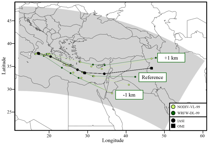
Figure 1 Satellite trajectory of the Mount Etna volcanic plume (black line) built by combining information from the IASI and OMI instruments, and the CHIMERE-simulated trajectory depending on the SO₂ injection altitude of emissions (light and dark green lines denote NODIV-VL-99 and WRFW-DL-99, respectively). The gray area represents the CHIMERE simulation domain, and the white triangle indicates Mount Etna's location.

2.2 Discretization of transport

The total concentration for all species combined is represented using C (number of gas particles per unit volume; $\mathrm{molec}.{\mathrm{m}}^{-\mathrm{3}}$; corresponding to air density), the concentration of a particular species s is denoted as C_s (number of molecules of species s per unit volume; $\mathrm{molec}.{\mathrm{m}}^{-\mathrm{3}}$) and the mixing ratio for species s is denoted as ${\mathit{\alpha }}_s=\frac{C_s}{C}$. The continuity equation for the motion of air is as follows:

$$\begin{array}{}\text{(1)}& {\displaystyle \frac{\partial C}{\partial t}}+\mathrm{\nabla }\left(\mathbf{\Phi }\right)=\mathrm{0},\end{array}$$

where Φ=Cu is the flux of air molecules.

In the following equations, i,j and k are the indices for the two horizontal directions and the vertical direction, respectively, and F_k+½ is the mass flux through the top of layer k, which is positively oriented for upward fluxes. Similarly the horizontal mass fluxes through lateral cell boundaries, which are positively oriented towards increasing i and j values, are denoted as $F_{i+\frac{\mathrm{1}}{\mathrm{2}},j,k}$ and $F_{i,j,k}$, respectively. The mass flux components need to verify the discretized form of Eq. (1):

$$\begin{array}{}\text{(2)}& \begin{array}{rl}{\displaystyle \frac{\partial C_{i,j,k}}{\partial t}}& +\left(F_{i,j,k+\frac{\mathrm{1}}{\mathrm{2}}}-F_{i,j,k-\frac{\mathrm{1}}{\mathrm{2}}}\right)+\left(F_{i+\frac{\mathrm{1}}{\mathrm{2}},j,k}-F_{i-\frac{\mathrm{1}}{\mathrm{2}},j,k}\right)\\ & +\left(F_{i,j+\frac{\mathrm{1}}{\mathrm{2}},k}-F_{i,j-\frac{\mathrm{1}}{\mathrm{2}},k}\right)=\mathrm{0}\end{array}\end{array}$$

The continuity equation for species s is as follows:

$$\begin{array}{}\text{(3)}& {\displaystyle \frac{\partial C_s}{\partial t}}+\mathrm{\nabla }\left({\mathbf{\Phi }}_s\right)=\mathrm{0},\end{array}$$

or equivalently

$$\begin{array}{}\text{(4)}& {\displaystyle \frac{\partial C_s}{\partial t}}+\mathrm{\nabla }\left({\mathit{\alpha }}_s\mathbf{\Phi }\right)=\mathrm{0}\end{array}$$

In CHIMERE, Eq. (4) is discretized as follows:

$$\begin{array}{}\text{(5)}& \begin{array}{rl}{\displaystyle \frac{\partial C_{s,i,j,k}}{\partial t}}+& \left({\overline{\mathit{\alpha }}}_{i,j,k+\frac{\mathrm{1}}{\mathrm{2}}}{F}_{i,j,k+\frac{\mathrm{1}}{\mathrm{2}}}-{\overline{\mathit{\alpha }}}_{i,j,k-\frac{\mathrm{1}}{\mathrm{2}}}{F}_{i,j,k-\frac{\mathrm{1}}{\mathrm{2}}}\right)\\ +& \left({\overline{\mathit{\alpha }}}_{i+\frac{\mathrm{1}}{\mathrm{2}},j,k}{F}_{i+\frac{\mathrm{1}}{\mathrm{2}},j,k}-{\overline{\mathit{\alpha }}}_{i-\frac{\mathrm{1}}{\mathrm{2}},j,k}{F}_{i-\frac{\mathrm{1}}{\mathrm{2}},j,k}\right)\\ +& \left({\overline{\mathit{\alpha }}}_{i,j+\frac{\mathrm{1}}{\mathrm{2}},k}{F}_{i,j+\frac{\mathrm{1}}{\mathrm{2}},k}-{\overline{\mathit{\alpha }}}_{i,j-\frac{\mathrm{1}}{\mathrm{2}},k}{F}_{i,j-\frac{\mathrm{1}}{\mathrm{2}},k}\right)=\mathrm{0},\end{array}\end{array}$$

where $\overline{\mathit{\alpha }}$ are the reconstituted values of the mixing ratio α on the facet indicated by the indices (${\overline{\mathit{\alpha }}}_{i,j,k+\frac{\mathrm{1}}{\mathrm{2}}}$ for the top facet of cell $i,j,k$, etc.). If the mass flux values F are such that Eq. (2) is exactly verified, Eq. (5) ensures that the mixing ratios α_s are not affected by mass–wind discrepancies: in particular, a species with an initially uniform mixing ratio will maintain it after transport is applied. This is why it is so critical for Eq. (2) to be verified exactly in chemistry transport models.

Equation (5) raises two important questions:

1. How should the interpolated mixing ratios ${\overline{\mathit{\alpha }}}_s$ be expressed (which is the task of the transport scheme)?

2. How should the exact verification of Eq. (2) be enforced to ensure the absence of mass–wind inconsistencies?

2.2.1 Vertical wind strategy

In CHIMERE, as in most other chemistry transport models (Emery et al., 2011), with the notable exception of chemistry transport modules that are embedded within a meteorological model and use the same grid and time step, as is most notably the case with WRF-Chem (Grell et al., 2005), the model does not have access to mass flux components $F_{i\pm \frac{\mathrm{1}}{\mathrm{2}},j\pm \frac{\mathrm{1}}{\mathrm{2}},k\pm \frac{\mathrm{1}}{\mathrm{2}}}$ and a density field C that verifies Eq. (2). This is a big problem when it comes to advecting species mixing ratios, as the fact that the CTM is able to transport species with Eq. (5) while maintaining the uniformity of initially uniform mixing ratios critically depends on this property (as we have seen above). Usually, chemistry transport models rely on the typical outputs of meteorological models, namely the instantaneous values of winds at the meteorological model cell boundaries, and instantaneous values of density. From these variables, it is possible to evaluate the mass fluxes through the CTM cell boundaries, obtaining interpolated mass flux values that are close to the “real” mass flux values from the model. We denote these values as ${\stackrel{\mathrm{̃}}{F}}_{i\pm \frac{\mathrm{1}}{\mathrm{2}},i\pm \frac{\mathrm{1}}{\mathrm{2}},i\pm \frac{\mathrm{1}}{\mathrm{2}}}$ and ${\stackrel{\mathrm{̃}}{C}}_{i,j,k}$.

With these interpolated values and after discretization in time is also performed, Eq. (2) is not verified, and it is turned into

$$\begin{array}{}\text{(6)}& \begin{array}{rl}{\displaystyle \frac{\partial {\stackrel{\mathrm{̃}}{C}}_{i,j,k}}{\partial t}}& +\left({\stackrel{\mathrm{̃}}{F}}_{i,j,k+\frac{\mathrm{1}}{\mathrm{2}}}-{\stackrel{\mathrm{̃}}{F}}_{i,j,k-\frac{\mathrm{1}}{\mathrm{2}}}\right)+\left({\stackrel{\mathrm{̃}}{F}}_{i+\frac{\mathrm{1}}{\mathrm{2}},j,k}-{\stackrel{\mathrm{̃}}{F}}_{i-\frac{\mathrm{1}}{\mathrm{2}},j,k}\right)\\ & +\left({\stackrel{\mathrm{̃}}{F}}_{i,j+\frac{\mathrm{1}}{\mathrm{2}},k}-{\stackrel{\mathrm{̃}}{F}}_{i,j-\frac{\mathrm{1}}{\mathrm{2}},k}\right)=-{\mathit{\epsilon }}_{i,j,k},\end{array}\end{array}$$

where ${\mathit{\epsilon }}_{i,j,k}$ is a spurious matter creation term due to mass–wind inconsistencies in the interpolated density and mass flux values from the meteorological model. ${\mathit{\epsilon }}_{i,j,k}$ depends on the resolution of the meteorological model (which is identical for all of our simulations) and on the resolution of the chemistry transport model; thus, this error term, which essentially traduces divergence errors due to interpolation, depends on the vertical resolution of the model. It is identical between simulations that have the exact same number of domains. Choosing interpolation strategies that reduce this error term is a promising path to mitigating excessive vertical diffusion, as discussed in Emery et al. (2011), but this is not investigated here.

As discussed above, the wind in CHIMERE is normally reconstructed from the bottom to the top of the model in order to prevent mass–wind inconsistency issues.

To enforce Eq. (2), reconstructed vertical fluxes ${\stackrel{\mathrm{‾}}{F}}_{i,j,k+\frac{\mathrm{1}}{\mathrm{2}}}$ are produced from the following constraints:

$$\begin{array}{}\text{(7a)}& {\displaystyle }{\stackrel{\mathrm{‾}}{F}}_{i,j,\frac{\mathrm{1}}{\mathrm{2}}}=\mathrm{0}\text{(7b)}& {\displaystyle }\begin{array}{rl}{\stackrel{\mathrm{‾}}{F}}_{i,j,k+\frac{\mathrm{1}}{\mathrm{2}}}& ={\stackrel{\mathrm{‾}}{F}}_{i,j,k-\frac{\mathrm{1}}{\mathrm{2}}}+\left({\stackrel{\mathrm{̃}}{F}}_{i-\frac{\mathrm{1}}{\mathrm{2}},j,k}-{\stackrel{\mathrm{̃}}{F}}_{i+\frac{\mathrm{1}}{\mathrm{2}},j,k}\right)\\ & +\left({\stackrel{\mathrm{̃}}{F}}_{i,j-\frac{\mathrm{1}}{\mathrm{2}},k}-{\stackrel{\mathrm{̃}}{F}}_{i,j+\frac{\mathrm{1}}{\mathrm{2}},k}\right)-{\displaystyle \frac{\partial {\stackrel{\mathrm{̃}}{C}}_{i,j,k}}{\partial t}}\end{array}\end{array}$$

Equation (7a) gives the boundary condition to the vertical mass flux reconstruction (no incoming mass flux of air comes from the ground surface). Equation (7b) ensures that, in each CTM cell and over one CTM time step, Eq. (2) is strictly verified (in the form of Eq. 7b) and Eq. (5) can be integrated using the interpolated horizontal fluxes ${\stackrel{\mathrm{̃}}{F}}_{i\pm \frac{\mathrm{1}}{\mathrm{2}},j\pm \frac{\mathrm{1}}{\mathrm{2}},k}$ and the reconstructed vertical fluxes ${\stackrel{\mathrm{‾}}{F}}_{i,j,k\pm \frac{\mathrm{1}}{\mathrm{2}}}$. This traditional approach will be labeled “NODIV” (for NO DIVergence) hereinafter.

In this study, we introduce and test a new approach that permits the user to bypass the need for a reconstructed vertical mass flux and work directly with the interpolated vertical mass fluxes ${\stackrel{\mathrm{̃}}{F}}_{i,j,k+\frac{\mathrm{1}}{\mathrm{2}}}$ while still maintaining the conservation of uniform mixing ratios. To explain this approach, we need to expand Eq. (5) as follows:

$$\begin{array}{}\text{(8)}& \begin{array}{rl}{\displaystyle \frac{\partial C_{s,i,j,k}}{\partial t}}+& \left(\mathit{\delta }{\overline{\mathit{\alpha }}}_{i,j,k+\frac{\mathrm{1}}{\mathrm{2}}}{\stackrel{\mathrm{̃}}{F}}_{i,j,k+\frac{\mathrm{1}}{\mathrm{2}}}-\mathit{\delta }{\overline{\mathit{\alpha }}}_{i,j,k-\frac{\mathrm{1}}{\mathrm{2}}}{\stackrel{\mathrm{̃}}{F}}_{i,j,k-\frac{\mathrm{1}}{\mathrm{2}}}\right)\\ & +\left(\mathit{\delta }{\overline{\mathit{\alpha }}}_{i+\frac{\mathrm{1}}{\mathrm{2}},j,k}{\stackrel{\mathrm{̃}}{F}}_{i+\frac{\mathrm{1}}{\mathrm{2}},j,k}-\mathit{\delta }{\overline{\mathit{\alpha }}}_{i-\frac{\mathrm{1}}{\mathrm{2}},j,k}{\stackrel{\mathrm{̃}}{F}}_{i-\frac{\mathrm{1}}{\mathrm{2}},j,k}\right)\\ & +\left(\mathit{\delta }{\overline{\mathit{\alpha }}}_{i,j+\frac{\mathrm{1}}{\mathrm{2}},k}{\stackrel{\mathrm{̃}}{F}}_{i,j+\frac{\mathrm{1}}{\mathrm{2}},k}-\mathit{\delta }{\overline{\mathit{\alpha }}}_{i,j-\frac{\mathrm{1}}{\mathrm{2}},k}{\stackrel{\mathrm{̃}}{F}}_{i,j-\frac{\mathrm{1}}{\mathrm{2}},k}\right)\\ & +{\mathit{\alpha }}_{i,j,k}\left[\left({\stackrel{\mathrm{̃}}{F}}_{i,j,k+\frac{\mathrm{1}}{\mathrm{2}}}-{\stackrel{\mathrm{̃}}{F}}_{i,j,k-\frac{\mathrm{1}}{\mathrm{2}}}\right)\right.\\ & +\left({\stackrel{\mathrm{̃}}{F}}_{i+\frac{\mathrm{1}}{\mathrm{2}},j,k}-{\stackrel{\mathrm{̃}}{F}}_{i-\frac{\mathrm{1}}{\mathrm{2}},j,k}\right)\\ & \left.+\left({\stackrel{\mathrm{̃}}{F}}_{i,j+\frac{\mathrm{1}}{\mathrm{2}},k}-{\stackrel{\mathrm{̃}}{F}}_{i,j-\frac{\mathrm{1}}{\mathrm{2}},k}\right)\right]=\mathrm{0},\end{array}\end{array}$$

where $\mathit{\delta }{\overline{\mathit{\alpha }}}_{i,j,k+\frac{\mathrm{1}}{\mathrm{2}}}={\overline{\mathit{\alpha }}}_{i,j,k+\frac{\mathrm{1}}{\mathrm{2}}}-{\mathit{\alpha }}_{i,j,k}$, and analogous definitions are used for the other $\mathit{\delta }\overline{\mathit{\alpha }}$ terms. Injecting Eq. (6) into Eq. (8) we obtain the following:

$$\begin{array}{}\text{(9)}& \begin{array}{rl}{\displaystyle \frac{\partial {\mathit{\alpha }}_{s,i,j,k}{\stackrel{\mathrm{̃}}{C}}_{i,j,k}}{\partial t}}+& \left(\mathit{\delta }{\overline{\mathit{\alpha }}}_{i,j,k+\frac{\mathrm{1}}{\mathrm{2}}}{\stackrel{\mathrm{̃}}{F}}_{i,j,k+\frac{\mathrm{1}}{\mathrm{2}}}-\mathit{\delta }{\overline{\mathit{\alpha }}}_{i,j,k-\frac{\mathrm{1}}{\mathrm{2}}}{\stackrel{\mathrm{̃}}{F}}_{i,j,k-\frac{\mathrm{1}}{\mathrm{2}}}\right)\\ +& \left(\mathit{\delta }{\overline{\mathit{\alpha }}}_{i+\frac{\mathrm{1}}{\mathrm{2}},j,k}{\stackrel{\mathrm{̃}}{F}}_{i+\frac{\mathrm{1}}{\mathrm{2}},j,k}-\mathit{\delta }{\overline{\mathit{\alpha }}}_{i-\frac{\mathrm{1}}{\mathrm{2}},j,k}{\stackrel{\mathrm{̃}}{F}}_{i-\frac{\mathrm{1}}{\mathrm{2}},j,k}\right)\\ +& \left(\mathit{\delta }{\overline{\mathit{\alpha }}}_{i,j+\frac{\mathrm{1}}{\mathrm{2}},k}{\stackrel{\mathrm{̃}}{F}}_{i,j+\frac{\mathrm{1}}{\mathrm{2}},k}-\mathit{\delta }{\overline{\mathit{\alpha }}}_{i,j-\frac{\mathrm{1}}{\mathrm{2}},k}{\stackrel{\mathrm{̃}}{F}}_{i,j-\frac{\mathrm{1}}{\mathrm{2}},k}\right)\\ -& {\mathit{\alpha }}_{s,i,j,k}\left[{\displaystyle \frac{\partial {\stackrel{\mathrm{̃}}{C}}_{i,j,k}}{\partial t}}+{\mathit{\epsilon }}_{i,j,k}\right]=\mathrm{0}\end{array}\end{array}$$

After simplification, this becomes

$$\begin{array}{}\text{(10)}& \begin{array}{rl}{\stackrel{\mathrm{̃}}{C}}_{i,j,k}{\displaystyle \frac{\partial {\mathit{\alpha }}_{s,i,j,k}}{\partial t}}+& \left(\mathit{\delta }{\overline{\mathit{\alpha }}}_{i,j,k+\frac{\mathrm{1}}{\mathrm{2}}}{\stackrel{\mathrm{̃}}{F}}_{i,j,k+\frac{\mathrm{1}}{\mathrm{2}}}-\mathit{\delta }{\overline{\mathit{\alpha }}}_{i,j,k-\frac{\mathrm{1}}{\mathrm{2}}}{\stackrel{\mathrm{̃}}{F}}_{i,j,k-\frac{\mathrm{1}}{\mathrm{2}}}\right)\\ +& \left(\mathit{\delta }{\overline{\mathit{\alpha }}}_{i+\frac{\mathrm{1}}{\mathrm{2}},j,k}{\stackrel{\mathrm{̃}}{F}}_{i+\frac{\mathrm{1}}{\mathrm{2}},j,k}-\mathit{\delta }{\overline{\mathit{\alpha }}}_{i-\frac{\mathrm{1}}{\mathrm{2}},j,k}{\stackrel{\mathrm{̃}}{F}}_{i-\frac{\mathrm{1}}{\mathrm{2}},j,k}\right)\\ +& \left(\mathit{\delta }{\overline{\mathit{\alpha }}}_{i,j+\frac{\mathrm{1}}{\mathrm{2}},k}{\stackrel{\mathrm{̃}}{F}}_{i,j+\frac{\mathrm{1}}{\mathrm{2}},k}-\mathit{\delta }{\overline{\mathit{\alpha }}}_{i,j-\frac{\mathrm{1}}{\mathrm{2}},k}{\stackrel{\mathrm{̃}}{F}}_{i,j-\frac{\mathrm{1}}{\mathrm{2}},k}\right)\\ -& {\mathit{\alpha }}_{s,i,j,k}{\mathit{\epsilon }}_{i,j,k}=\mathrm{0}\end{array}\end{array}$$

From Eq. (10), it can be observed that if the mixing ratio ${\mathit{\alpha }}_{i,j,k}=\frac{C_{s,i,j,k}}{{\stackrel{\mathrm{̃}}{C}}_{i,j,k}}$ is initially uniform, all of the $\mathit{\delta }\overline{\mathit{\alpha }}$ terms vanish. Here, the mixing ratio uniformity will be maintained after integrating Eq. (8) if, and only if, the mass–wind inconsistency term ${\mathit{\epsilon }}_{i,j,k}$ is zero. This is already well known, but with this formulation we can obtain a modified version of Eq. (5) that will enforce mixing ratio preservation even if the mass–wind inconsistency term ${\mathit{\epsilon }}_{i,j,k}$ is not zero:

$$\begin{array}{}\text{(11)}& \begin{array}{rl}{\displaystyle \frac{\partial C_{s,i,j,k}}{\partial t}}+& \left({\overline{\mathit{\alpha }}}_{i,j,k+\frac{\mathrm{1}}{\mathrm{2}}}{\stackrel{\mathrm{̃}}{F}}_{i,j,k+\frac{\mathrm{1}}{\mathrm{2}}}-{\overline{\mathit{\alpha }}}_{i,j,k-\frac{\mathrm{1}}{\mathrm{2}}}{\stackrel{\mathrm{̃}}{F}}_{i,j,k-\frac{\mathrm{1}}{\mathrm{2}}}\right)\\ +& \left({\overline{\mathit{\alpha }}}_{i+\frac{\mathrm{1}}{\mathrm{2}},j,k}{\stackrel{\mathrm{̃}}{F}}_{i+\frac{\mathrm{1}}{\mathrm{2}},j,k}-{\overline{\mathit{\alpha }}}_{i-\frac{\mathrm{1}}{\mathrm{2}},j,k}{F}_{i-\frac{\mathrm{1}}{\mathrm{2}},j,k}\right)\\ +& \left({\overline{\mathit{\alpha }}}_{i,j+\frac{\mathrm{1}}{\mathrm{2}},k}{\stackrel{\mathrm{̃}}{F}}_{i,j+\frac{\mathrm{1}}{\mathrm{2}},k}-{\overline{\mathit{\alpha }}}_{i,j-\frac{\mathrm{1}}{\mathrm{2}},k}{\stackrel{\mathrm{̃}}{F}}_{i,j-\frac{\mathrm{1}}{\mathrm{2}},k}\right)\\ & +C_{s,i,j,k}{\displaystyle \frac{{\mathit{\epsilon }}_{i,j,k}}{{\stackrel{\mathrm{̃}}{C}}_{i,j,k}}}=\mathrm{0}\end{array}\end{array}$$

Equation (11) will be solved in the simulation labeled WRFW, with mass fluxes directly interpolated from the meteorological model winds in the three directions. It must be noted that mass conservation is not enforced by this equation: the additional term $C_{s,i,j,k}\frac{{\mathit{\epsilon }}_{i,j,k}}{{\stackrel{\mathrm{̃}}{C}}_{i,j,k}}$ is an artificial mass production or loss term that breaks the conservation of total mass of species s over the entire domain. If we summarize this part, the NODIV simulation (classical approach) enforces tracer mass conservation and tracer mixing ratio conservation. This is obtained at the expense of unrealistic vertical transport, as mass–wind consistency is, in this approach, enforced by artificially modifying the vertical mass fluxes. However, this reconstructed wind is significantly different from WRF input data while reaching the upper troposphere (Fig. S1 in the Supplement), and this approach induces excessive transport across the tropopause. Vertical wind distribution comparisons between WRFW and NODIV strategies (Fig. S1 in the Supplement) show that more vertical diffusion is expected in the NODIV strategy in the upper troposphere. The WRFW approach that we propose here, in comparison, permits mixing ratio conservation and the use of realistic vertical mass fluxes at the expense of mass conservation. While nonconservation of mass is obviously a significant drawback for a transport strategy, we will quantify the problem of nonconservation of mass as well as the issues introduced by the artificial reconstruction of vertical mass fluxes in the representation of vertical transport in the NODIV approach (Fig. 3).

2.2.2 Vertical advection scheme

After discretizing the advection equation for species s in the form of Eq. (5), the point of the vertical transport scheme is to estimate the reconstructed mixing ratios ${\overline{\mathit{\alpha }}}_{i,j,k+\frac{\mathrm{1}}{\mathrm{2}}}$, for k varying between one and the number of vertical levels nz. The most simple way of doing so is the Godunov donor-cell scheme, simply evaluating ${\overline{\mathit{\alpha }}}_{s,i,j,k+\frac{\mathrm{1}}{\mathrm{2}}}$ as

$$\begin{array}{}\text{(12)}& {\displaystyle }{\overline{\mathit{\alpha }}}_{s,i,j,k+\frac{\mathrm{1}}{\mathrm{2}}}={\mathit{\alpha }}_{s,i,j,k}\mathrm{if}{\mathrm{F}}_{\mathrm{i},\mathrm{j},\mathrm{k}+\frac{\mathrm{1}}{\mathrm{2}}}>\mathrm{0}\text{(13)}& {\displaystyle }{\overline{\mathit{\alpha }}}_{s,i,j,k+\frac{\mathrm{1}}{\mathrm{2}}}={\mathit{\alpha }}_{s,i,j,k+\mathrm{1}}\mathrm{if}{\mathrm{F}}_{\mathrm{i},\mathrm{j},\mathrm{k}+\frac{\mathrm{1}}{\mathrm{2}}}<\mathrm{0}\end{array}$$

This first-order scheme is mass conservative but extremely diffusive. Therefore, it is important to find more accurate ways of estimating ${\overline{\mathit{\alpha }}}_{s,i,j,k+\frac{\mathrm{1}}{\mathrm{2}}}$.

The Van Leer (1977) scheme

The second-order slope-limited scheme of Van Leer (1977) brought to our notation yields the following expression of ${\overline{\mathit{\alpha }}}_{s,k+\frac{\mathrm{1}}{\mathrm{2}}}$ (for $F_{i,j,k+\frac{\mathrm{1}}{\mathrm{2}}}>\mathrm{0}$):

$$\begin{array}{}\text{(14)}& \begin{array}{rl}{\overline{\mathit{\alpha }}}_{s,k+\frac{\mathrm{1}}{\mathrm{2}}}& ={\mathit{\alpha }}_{s,k}+{\displaystyle \frac{\mathrm{1}-\mathit{\nu }}{\mathrm{2}}}\mathrm{sign}\left({\mathit{\alpha }}_{s,k+\mathrm{1}}-{\mathit{\alpha }}_{s,k}\right)\mathrm{Min}({\displaystyle \frac{\mathrm{1}}{\mathrm{2}}}\left|{\mathit{\alpha }}_{s,k+\mathrm{1}}\right.\\ & \left.-{\mathit{\alpha }}_{s,k-\mathrm{1}}\right|,\mathrm{2}\left|{\mathit{\alpha }}_{s,k+\mathrm{1}}-{\mathit{\alpha }}_{s,k}\right|,\mathrm{2}\left|{\mathit{\alpha }}_{s,k}-{\mathit{\alpha }}_{s,k-\mathrm{1}}\right|),\end{array}\end{array}$$

where $\mathit{\nu }=\frac{F_{i,j,k+\frac{\mathrm{1}}{\mathrm{2}}}}{{\mathit{\rho }}_{i,j,k}{V}_{i,j,k}}$ is the Courant number for the donor cell $i,j,k$, with $V_{i,j,k}$ being its volume: if ν>1, more mass leaves the cell than the mass that was initially present, and the Courant–Friedrichs–Lewy condition is violated, yielding numerical instability. Equation (14) is not applied in the case of a local extremum ($\left({\mathit{\alpha }}_{s,k}-{\mathit{\alpha }}_{s,k-\mathrm{1}}\right)\left({\mathit{\alpha }}_{s,k+\mathrm{1}}-{\mathit{\alpha }}_{s,k}\right)\le \mathrm{0}$). In this case, ${\overline{\mathit{\alpha }}}_{s,k+\frac{\mathrm{1}}{\mathrm{2}}}={\mathit{\alpha }}_{s,k}$ is imposed, and the scheme falls back to the simple Godunov donor-cell formulation (Eq. 12). This second-order scheme has been used for decades in chemistry transport modeling, as it is a good tradeoff between reasonably weak diffusion, at least compared with simpler schemes such as the Godunov donor-cell scheme, and it is computationally cheaper than higher-order schemes such as the piecewise parabolic method (Colella and Woodward, 1984).

The Després and Lagoutière (1999) scheme

The scheme of Després and Lagoutière (1999) is defined by their Eqs. (2) to (4). If $F_{i,j,k+\frac{\mathrm{1}}{\mathrm{2}}}>\mathrm{0}$, these equations brought to our notation, adapted to the flux form of Eq. (5) and ignoring the i,j indices to shorten the expression, give the following:

$$\begin{array}{}\text{(15)}& \begin{array}{rl}{\overline{\mathit{\alpha }}}_{s,k+\frac{\mathrm{1}}{\mathrm{2}}}& ={\mathit{\alpha }}_{s,k}+{\displaystyle \frac{\mathrm{1}-\mathit{\nu }}{\mathrm{2}}}\mathrm{Max}\\ & \left[\mathrm{0},\mathrm{Min}\left({\displaystyle \frac{\mathrm{2}}{\mathit{\nu }}}{\displaystyle \frac{{\mathit{\alpha }}_{s,k}-{\mathit{\alpha }}_{s,k-\mathrm{1}}}{{\mathit{\alpha }}_{s,k+\mathrm{1}}-{\mathit{\alpha }}_{s,k}}},{\displaystyle \frac{\mathrm{2}}{\mathrm{1}-\mathit{\nu }}}\right)\right]\\ & \times \left({\mathit{\alpha }}_{s,k+\mathrm{1}}-{\mathit{\alpha }}_{s,k}\right),\end{array}\end{array}$$

with the same notation as for the Van Leer (1977) scheme (above). As above, Eq. (15) is not applied in the case of a local extremum ($\left({\mathit{\alpha }}_{s,k}-{\mathit{\alpha }}_{s,k-\mathrm{1}}\right)\left({\mathit{\alpha }}_{s,k+\mathrm{1}}-{\mathit{\alpha }}_{s,k}\right)\le \mathrm{0}$). In this case, ${\overline{\mathit{\alpha }}}_{s,k+\frac{\mathrm{1}}{\mathrm{2}}}={\mathit{\alpha }}_{s,k}$ is imposed, and the scheme falls back to the simple Godunov donor-cell formulation (Eq. 12). As stated by its authors, this scheme is anti-diffusive. Unlike other schemes, such as the Van Leer (1977) scheme described above, two unusual choices have been made by the authors in order to minimize diffusion by the advection scheme:

• their scheme is accurate only to the first order,

• the scheme is linearly unstable, but nonlinearly stable (their Theorem 1).

The authors' idea was to make the interpolated value ${\overline{\mathit{\alpha }}}_{s,k+\frac{\mathrm{1}}{\mathrm{2}}}$ as close as possible to the downstream value (${\mathit{\alpha }}_{s,k+\mathrm{1}}$ if the flux is upward). This property is desirable because it is the key property in order to reduce numerical diffusion as much as mathematically possible while still maintaining the scheme stability. The authors present 1D case studies with their scheme obtaining extremely interesting results: fields that are initially concentrated on one single cell do not occupy more than three cells even after a long advection time (their Fig. 2); sharp gradients are very well preserved (their Fig. 1); and, more unexpectedly due to its anti-diffusive character, the scheme also performs well in maintaining the shape of concentration fields with an initially smooth concentration gradient. After extensive testing, these authors also suggested (their Conjecture 1) that convergence of the simulated values towards exact values occurs, even if the time step is reduced before the space step: in simpler terms, this means that the scheme performs very well even at small Courant–Friedrichs–Levy values, which is a property that is not shared by most advection schemes.

Table 1 List of the various model parameters tested, allowing for a total of 12 distinct simulations to be performed.

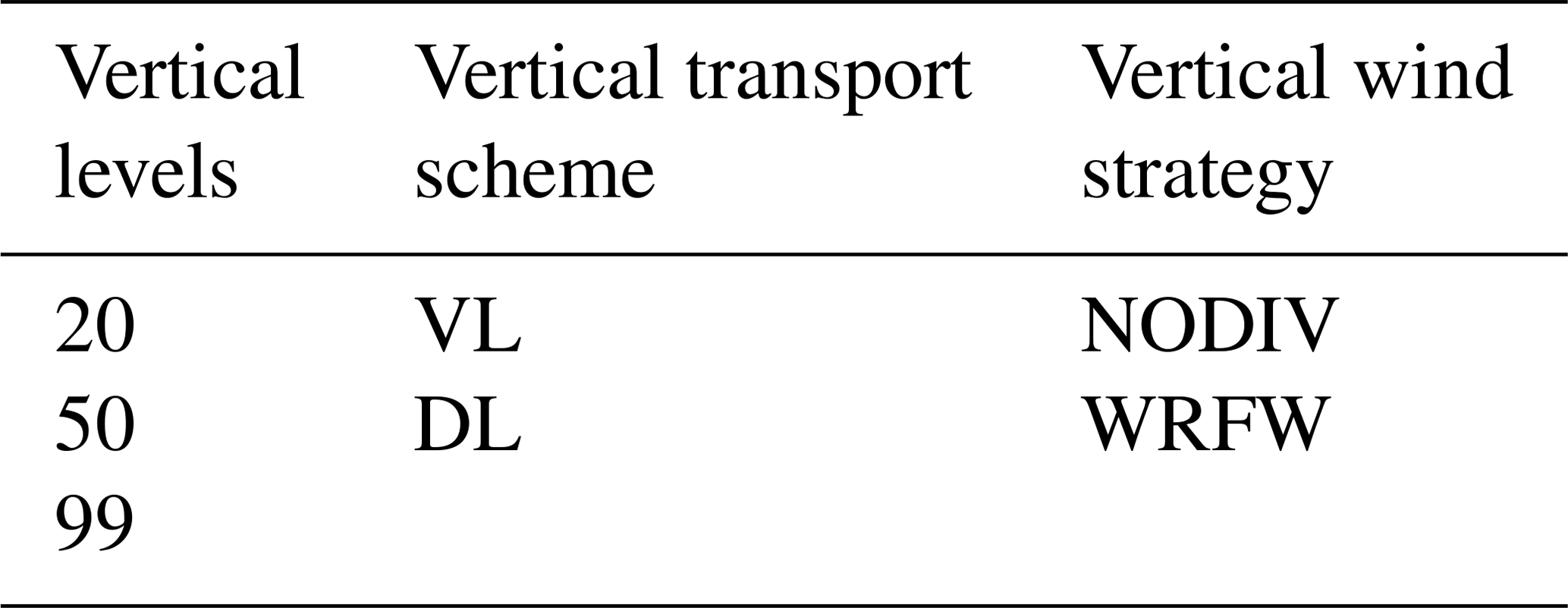
2.2.3 Model parameters tested

The various possible parameter combinations between the vertical flux (NODIV for reconstructed vertical fluxes and WRFW for interpolated vertical mass flux), the vertical transport scheme (VL for Van Leer, 1977 and DL for Després and Lagoutière, 1999) and the number of vertical levels (20, 50 and 99) are summarized in Table 1. Following all of the possible combinations between these parameters, 12 simulations were performed.

2.3 SO₂ emissions from the 18 March 2012 eruption of Mount Etna

The time and altitude profiles for the injection of SO₂ into the atmosphere (Table 2) were obtained using SO₂ flux measurement data from the ground-based DOAS FLAME (Differential Optical Absorption Spectroscopy FLux Automatic MEasurements) scanning network (e.g., Salerno et al., 2018). This method accurately measures SO₂ fluxes during passive degassing and effusive and explosive eruptive activity using a plume height inverted by an empirical relationship between the plume height and wind speed (Salerno et al., 2009). In explosive paroxysmal events, as in the case in this study, the plume is ejected to higher altitudes, and this linear height–wind relationship can not be used. Mass flux is retrieved in post-processing using the plume height estimated by visual camera and/or satellite retrieval.

On 18 March 2012, between 06:00 and 15:00 UTC, a total SO₂ emission of 2.94 kt was reported using this method. A total of 91 % of this mass was released within 2 h at an altitude of around 12 km. In CHIMERE, emissions were distributed into a single model cell based on altitude injection. Two alternates cases were tested, considering −1 and +1 km for all of the injection heights defined in Table 2.

Table 2 SO₂ hourly flux (kg s⁻¹) estimates used as input for the CHIMERE model.

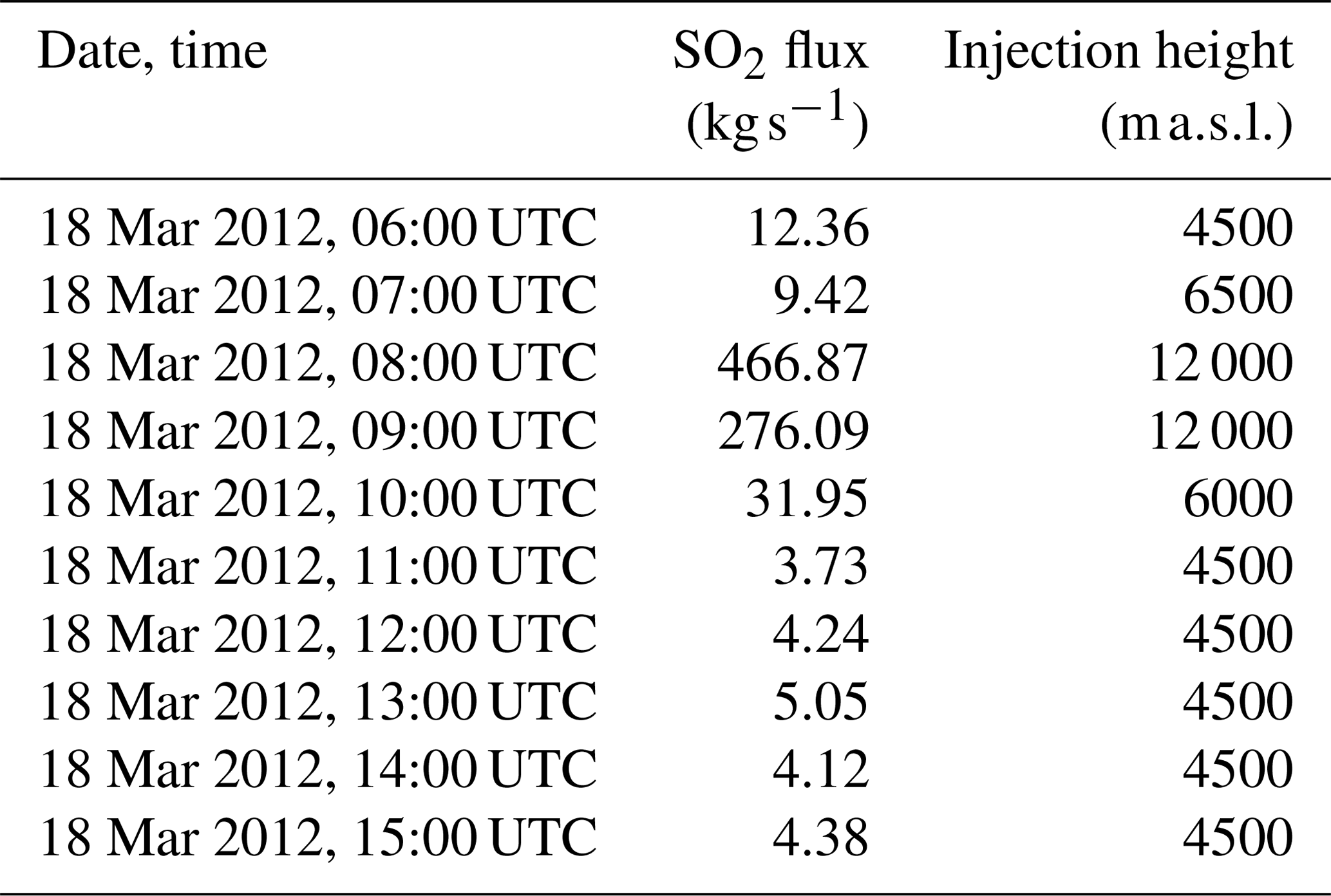
Table 3 IASI and OMI soundings list. λ_OBS,i (longitude) and Φ_OBS,i (latitude) represent the plume's column with the highest SO₂ content coordinates. λ_thr,i is the limit longitude that has been set as limit between the eastern and western plumes in Sect. 3.5.

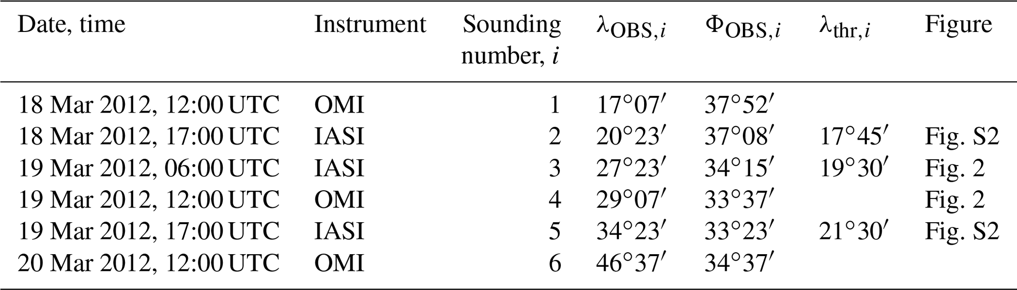
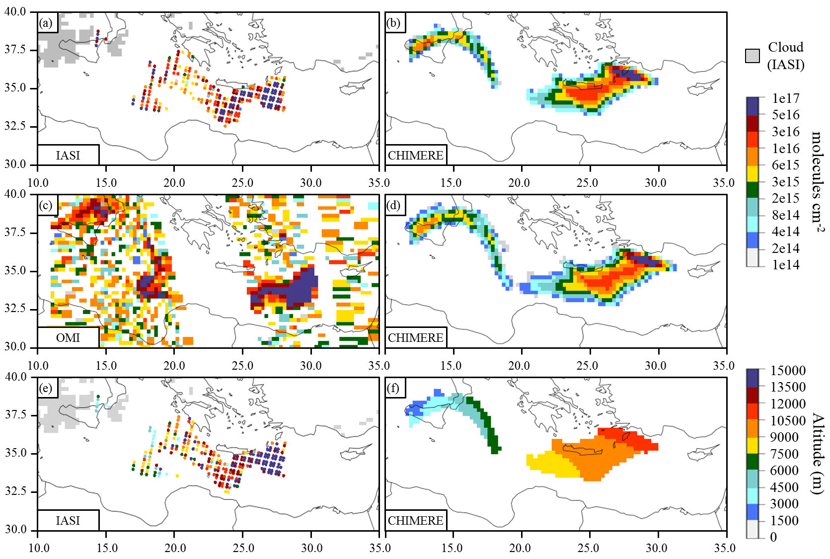
Figure 2 The IASI SO₂ plume (a), the OMI SO₂ plume (c), and the respective IASI and OMI soundings for 19 March 2012 at 06:00 and 12:00 UTC (3 and 4 in Table 3). The CHIMERE SO₂ plume (b, d), in molecules per square centimeter ($\mathrm{molec}.{\mathrm{cm}}^{-\mathrm{2}}$), corresponding to the IASI and OMI soundings. The IASI SO₂ altitude (e) and the CHIMERE SO₂ maximum concentrations' altitudes (f), in meters (m), for 19 March 2012 at 06:00 UTC. In this example, the CHIMERE simulation WRFW-DL-20 is displayed. CHIMERE and OMI data are represented on OMI's 0.25^∘ × 0.25^∘ resolution grid. Clouds are based on Advanced Very High Resolution Radiometer (AVHRR) data for IASI. A log scale is used to better visualized CHIMERE simulations, but values under 3×10¹⁵ (∼0.1 DU) are below satellite detection limits.

2.4 The IASI and OMI instruments

To evaluate the numerical parameters tested in our simulations, satellite-based information was used to evaluate the SO₂ plume's transport and vertical distribution. SO₂ column observations were provided by the Infrared Atmospheric Sounding Interferometer instrument (IASI) onboard the Metop-A European satellite and the Ozone Monitoring Instrument (OMI) onboard the Aura NASA satellite (Levelt et al., 2006; McCormick et al., 2013). The IASI instrument operates between 3.7 and 15.5 µm, including SO₂ ν₁ (around 8.7 µm) and ν₃ (7.3 µm) bands (Carboni et al., 2012). The IASI scheme (Carboni et al., 2012, 2016) provides the SO₂ total column content and plume altitude. This product is shown in Fig. 2 along with OMI SO₂ columns and CHIMERE outputs. In our analysis, we used IASI retrievals from 18 March at 17:00 UTC (Fig. S2), 19 March at 06:00 UTC (Fig. 2) and 19 March at 17:00 UTC (Fig. S3). OMI data were obtained from the NASA Giovanni platform². OMI data were provided with a 0.25^∘ × 0.25^∘ resolution and daily coverage at 12:00 UTC for 18, 19 and 20 March over the studied area. All instruments soundings are given in Table 3.

3 Results and discussion

3.1 Impact of the injection altitude on plume transport

Alternative injection height scenarios were tested, which entailed either lifting or lowering the injection height at all times by 1 km, thereby lifting maximum injection heights up to 13 km or lowering minimum injection heights down to 11 km, respectively, compared with the 12 km level in the reference simulation. These tests have shown that plume trajectories are strongly sensitive to this parameter (Fig. 1), which is an effect of wind shear. For each satellite sounding, the coordinates of the model column with the strongest vertically integrated SO₂ content ($\mathrm{molec}.{\mathrm{SO}}_{\mathrm{2}}{\mathrm{cm}}^{-\mathrm{2}}$) were selected and were considered as SO₂ plume centroids. With the three available IASI soundings and the three available OMI soundings, this gives six points on the satellite-retrieved Mount Etna plume trajectory that range from Sicily to western Iran. The IASI and OMI centroids and the constructed plume trajectory are displayed in black in Fig. 4.

The simulation and satellite plumes' initial positions do not correspond to the Mount Etna location because the first OMI sounding is at 12:00 UTC on 18 March, 6 h after the beginning of the eruption. Compared with the trajectory reconstituted from OMI and IASI observations, the plume injected at 11 km seems to be transported too far towards the south, whereas the plume injected at 13 km appears to be shifted to the north compared with observations. This observation is largely independent of the model parameters (NODIV-VL-99 and WRFW-DL-99 are shown in Fig. 1), suggesting that the configuration with the maximum injection height at 12 km is the best configuration. Therefore, only this choice of injection height was retained for the rest of the study.

In addition, the sensitivity to injection vertical profile has been investigated using three options:

• injection to a unique altitude,

• injection with a full width at half maximum of 100 m, (Boichu et al., 2015)

• injection with a full width at half maximum of 300 m.

The tests were conducted with a 20-, 50- and 99-vertical-level resolution. These sensitivity tests showed little difference between the various cases, even at the 99-vertical-level resolution, with plumes close to trajectories and vertical diffusion. Injection at a unique altitude – consequently in a unique cell – was conserved and used to perform and evaluate the vertical diffusion strategies.

3.2 Evaluation of SO₂ dispersion with a similar vertical extent at injection

To evaluate the impact that the schemes and vertical resolution would have with a similar vertical extent at injection, new simulations were conducted that imposed an identical vertical distribution at the initial time (vertically spreading the emitted mass over the same thickness in the 50- and 99-level simulations as it had in the 20-level simulation). Simulations were conducted for 20, 50 and 99 vertical levels for the respective WRFW-DL and NODIV-VL parameters, resulting in a total of six simulations. The results are displayed in Fig. S5 in the Supplement. It can be seen in Fig. S5 (left) that all plumes have the same initial volume regardless of vertical resolution, which was not the case in the previous example (cf. Fig. 8a). With a larger vertical extent of the plume at injection, the volumes are higher than in the “unique cell injection” cases, but the resolution and transport scheme influence the evolution of plume in the same way (considering its volume). Figure S5 (right) shows the evolution of the SO₂ highest column vertical profile, similar to Fig. 7. This new set of experiments show that, even when getting rid of the initial distortion due to sharper injection profiles in the simulations with the most refined vertical distributions, the increase in plume volume is much slower in the 99-level simulations than in the 20-level simulations. The final volume is about 4 times smaller in the 99-level simulations compared with their 20-level counterparts. A similar factor is obtained for the volume reduction by changing the strategy from VL-NODIV to DL-REALW. In total, the final plume volume in the worst-case NODIV-VL-20 simulation is about 20 times larger than final plume volume in the best-case WRFW-DL-99 simulation. Figure S5 (right panel) shows that the WRFW-DL-99 simulation is able to reproduce plume thinning under the effect of wind shear, with the plume getting thinner at the end the simulation than it was at the beginning.

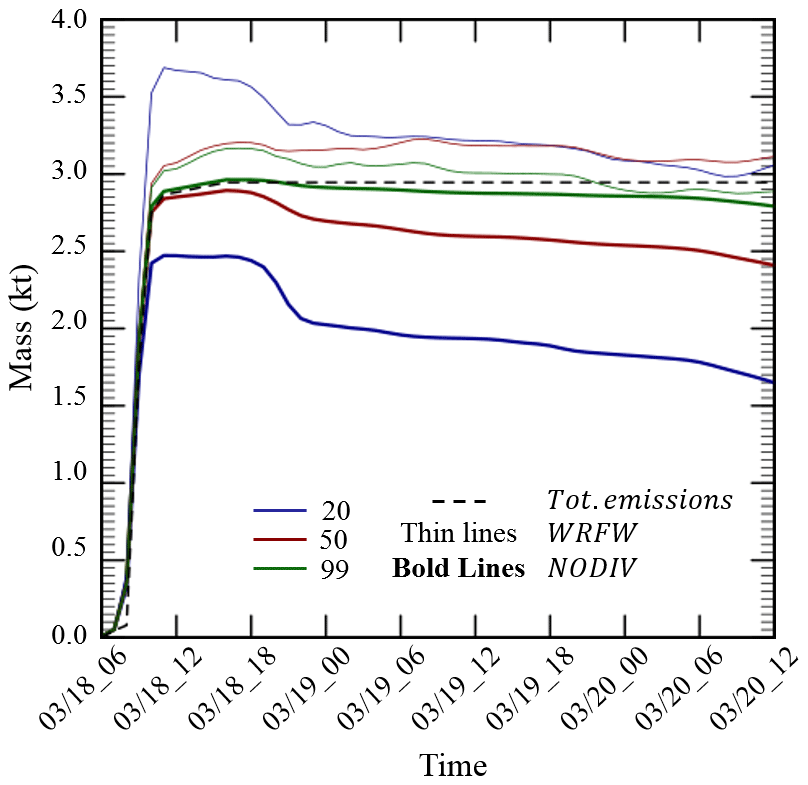
Figure 3 The SO₂ mass evolution in model domain (kilotons). The line color indicates the vertical level configuration, and the line thickness indicates the vertical wind strategy considered. The dotted line represents the cumulative SO₂ mass emitted during the Mount Etna eruption.

3.3 Mass conservation

Figure 3 shows the evolution of the total mass of tracer inside the simulation domain as a function of time. Several features from this figure require comment.

In the simulations with the reconstituted non-divergent wind field, substantial mass leak through the top of model can be observed as soon as the injection starts in the 20-level simulation (in which injection is carried out in the highest model level): the mass of tracer present in the domain never exceeds 85 % of the emitted mass. For the simulation with 50 vertical levels, this phenomenon is also visible. Another strong episode of mass leak through model top occurs in the simulations with 20 and 50 vertical levels and with reconstructed wind fields from 18 March at 18:00 UTC to 19 March at 00:00 UTC. This episodes causes an additional drop in tracer mass of 20 % in the simulation with 20 levels and 5 % in the simulation with 50 vertical levels. This leak episode also affects the simulation with 20 vertical levels and with interpolated wind fields, reducing the tracer mass concentration by about 10 % from 18 March at 18:00 UTC to 19 March at 00:00 UTC. In these three simulations (20 and 50 levels with non-divergent winds and 20 levels with interpolated winds), a continuous decreasing trend in tracer mass is observed throughout the simulation. This drop is directly attributable to leak through model top, as the tracer plume is far away from the horizontal boundaries of the domain.

As could be expected, the simulations with the WRFW wind strategy, due to the additional term in Eq. (11), do not enforce mass conservation. In theory, the additional term, designed to ensure mixing ratio conservation in spite of mass–wind inconsistencies, can result into either an artificial increase or an artificial decrease in simulated tracer mass. In the three simulations that are shown in Fig. 3, the amount of tracer present in the domain just after the end of the eruption overshoots the expected mass – by 20 % in the simulation with 20 vertical levels and by 10 % in the two simulations with a larger number of levels. No physical process can explain this overshoot, and it is directly attributable to the choice of lifting the mass conservation constraint in the formulation of transport in order to permit the use of a realistic wind field. If we take 19 March at 00:00 UTC as a reference time at which the eruption is terminated, the first strong event of leak through model top is also terminated, and we can observe that the mass evolution in all three WRFW simulations undergoes small variations from one hour to the next but remains confined to very narrow ranges: 3.3 to 3 kt for the simulation with 20 vertical levels, with a decreasing trend attributable to leakage through model top; 3.1 to 3.25 for the simulation with 50 levels; and 2.9 to 3.1 kt for the simulation with 99 vertical levels. The fact that these variations in total mass become marginal in this latter part of plume advection, when the plume is spread over a large geographic areas, reflects the fact that numerical errors in the evaluation of divergence mechanically tend to compensate for each other between neighboring cells so that their global impact on a plume that is dispersed over many cells is small.

3.4 Horizontal transport evaluation with the OMI and IASI instruments

In this section, we aim to determine how the various parameters tested (Table 1) have influenced the plume trajectory. The plume trajectories from simulations were constructed following the same methodology as described above for satellite data, using the corresponding satellite sounding time step and retaining the coordinates of the model column with the strongest vertically integrated SO₂ content. The trajectories of all 12 simulations are shown in Fig. 4a, with a color code that is aimed at highlighting the impact of the number of vertical levels on the diffusion. Figure 4b allows for the comparison of the influence of the vertical transport schemes (VL or DL), and Fig. 4c allows for the comparison of the influence of the various vertical wind strategies (NODIV or WRFW).

It can be observed that no significant differences between the vertical transport schemes nor the vertical wind strategy are found for the various 20-vertical-level simulations, except for the NODIV-VL-20 simulation which strongly diverges and split into two different plumes at OMI's last sounding. For the 50- and 99-vertical-level simulations, more differences are found, which are mainly controlled by the choice of vertical transport schemes (VL or DL). As for NODIV-VL-20, the NODIV-VL-50 simulation presents a split into two distinct SO₂ plumes for OMI's last sounding.

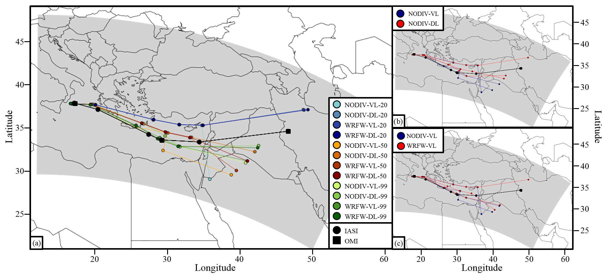
Figure 4 Mount Etna volcanic plume transport over the Mediterranean Sea after the 18 March 2012 eruption. The satellite trajectory (black line) was built by combining information from the IASI and OMI instruments. (a) Transport for all simulations, (b) plume transport highlighted according to the vertical scheme and (c) plume transport highlighted according to the vertical wind strategy. The points along the trajectories correspond to those listed in Table 3.

To conduct a more quantitative and synthetic analysis of the deviation between the observations and the model outputs, the geographic distance between the satellite observation centroids and the simulations centroids was calculated for every sounding. This calculation provided a satellite–model difference time series for each simulation. To better estimate the impact of the tested parameters, gap means were then calculated according to the simulations' parameters in order to separately evaluate the impact of each parameter choice on the accuracy of plume simulation. Results are displayed in Fig. 5a. A general mean value for each time series was calculated and is shown in Fig. 5a (last points on the time axis). As expected, gaps between the satellite and model centroids generally increase with time.

It can be seen that the DL vertical scheme has better agreement with the observations than the VL vertical scheme, with a respective mean gap of 189 and 316 km – with the NODIV wind strategy option fixed. The WRFW wind strategy also shows better agreement with soundings than the NODIV strategy, with a respective mean gap 230 and 316 km – with the VL vertical scheme fixed.

To complete the centroids' gap analysis, agreement between satellite measurements and model simulations in the zonal and meridional displacements of the centroids was calculated, as expressed in Eq. (16) for a given simulation (SIM):

$$\begin{array}{}\text{(16)}& \begin{array}{rl}& {\mathrm{\Delta }}_{(i,i-\mathrm{1}),\mathrm{SIM}}\left(\mathrm{km}\right)=\\ & R\sqrt{\begin{array}{c}{\cos }^{\mathrm{2}}\mathrm{\Phi }{\left(\mathrm{\Delta }{\mathit{\lambda }}_{\mathrm{SIM},(i,i-\mathrm{1})}-\mathrm{\Delta }{\mathit{\lambda }}_{\mathrm{OBS},(i,i-\mathrm{1})}\right)}^{\mathrm{2}}\\ +(\mathrm{\Delta }{\mathrm{\Phi }}_{\mathrm{OBS},(i,i-\mathrm{1})}-\mathrm{\Delta }{\mathrm{\Phi }}_{\mathrm{SIM},(i,i-\mathrm{1})}{)}^{\mathrm{2}}\end{array}},\end{array}\end{array}$$

where $\mathrm{\Delta }{\mathit{\lambda }}_{\mathrm{SIM},(i,i-\mathrm{1})}={\mathit{\lambda }}_{\mathrm{SIM},i}-{\mathit{\lambda }}_{\mathrm{SIM},i-\mathrm{1}}$, and $\mathrm{\Delta }{\mathit{\lambda }}_{\mathrm{OBS},(i,i-\mathrm{1})}={\mathit{\lambda }}_{\mathrm{OBS},i}-{\mathit{\lambda }}_{\mathrm{OBS},i-\mathrm{1}}$.

Here, i refers to sounding numbers (Table 3), λ_OBS,i and Φ_OBS,i refer to the geographic coordinates of the observed centroid for sounding i at time t_i (Table 3), λ_SIM,i and Φ_SIM,i refer to the coordinates of the simulated centroid, and R is the Earth's radius. In this case, we focus on the displacement of the plume between two successive observation points. The intention of Eq. (16) is to build an index that not only qualifies the distance between the observed and modeled trajectories but also the realism of the displacements followed between two successive satellite snapshots, giving penalties to simulations that would oscillate erratically around the observed trajectory and bonuses to simulations that would follow a realistic trajectory, although slightly shifted towards either side. Results are displayed in Fig. 5b, and a mean value for each time series has once again been calculated and is displayed in Fig. 5b (last boxes). It can be observed (as in the previous indicator case) that the DL vertical scheme and WRFW vertical wind strategy provide better results than the opposing VL and NODIV parameters, respectively. It can also be clearly seen for both criteria that the 99-vertical-level option shows the best results to both centroid position and trajectory comparisons to the satellite compared with the 50- or 20-vertical-level options.

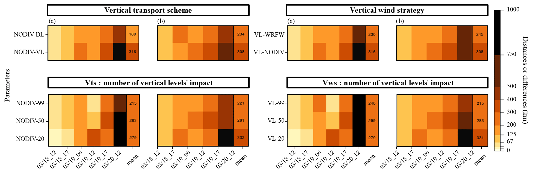
Figure 5 The left column shows the impact of the vertical transport scheme. The right column shows the impact of the vertical wind strategy. (a) Gap between the satellites and CHIMERE SO₂ plume centroids. (b) Differences between the SO₂ plume centroids' trajectories. To produce this figure, differences (in km) between the model and satellite plumes' centroids were calculated for each simulation, and the impact of each parameter was then evaluated by calculating the mean between the simulation and satellite differences. For instance, “NODIV-DL” (first line, left column) is the mean between “NODIV-DL-20”, “NODIV-DL-50” and “NODIV-DL-99”; “NODIV-99” (third line, left column) is the mean between “NODIV-DL-99” and “NODIV-VL-99”.

3.5 Comparison of the simulated plume vertical structure with the IASI-retrieved structure

IASI observations also provide the estimated altitude of the SO₂ plume for each pixel with a valid SO₂ retrieval (Fig. 2e), along with the corresponding uncertainty. For each of the three available IASI soundings (numbers 2, 3 and 5 in Table 3), we extracted the plume altitude and its associated uncertainty for the pixel with the highest SO₂ content. Comparison of this plume altitude with the same calculation made on the plume simulated by CHIMERE is shown in Fig. S4 (in the Supplement). For the first available IASI sounding, it can be observed that the concentration maximum altitude for CHIMERE soon after the Mount Etna eruption is consistent with the IASI altitude and is found within IASI uncertainties (12 100 m ± 900 m). Along with the trajectories shown in Fig. 1, this is an indication that the highest emission altitude of 12 km in Table 2 is realistic.

In the IASI dataset, a bimodal altitude distribution is observed, indicating the coexistence of two separate sub-plumes during this eruption: one located to the east at higher altitude and another located to the west at lower altitude (Fig. 2). This has also been observed in “AEROIASI-Sulphates” soundings in Sellitto et al. (2017) and Guermazi et al. (2019). This partition is due to the sharp separation between emissions at very high altitudes (≃12 km) and emissions below ≃7.5 km (Table 2) and to the fact that at the Mount Etna latitudinal wind shear is generally strong with steady westerly winds in the higher troposphere and more variable winds in the lower troposphere. As most of the SO₂ is emitted around ≃12 km (Table 2), most of the SO₂ mass is found in the eastern plume. From each available IASI observation of the plume (soundings 2, 3 and 5 in Table 2), a transitional longitude that separates the western plume from the eastern plume has been identified. These longitudes are given in Table 2 and can be compared to Figs. S2 and S3. The same longitudes have been used to separate the eastern and western plumes in the CHIMERE simulations. Figure 6 compares the altitude distribution between the CHIMERE simulations and IASI retrievals – 20-vertical-level simulations have been removed, because the coarse altitude resolution does not permit a useful representation of the maximum concentration's altitude distribution (see Fig. S4 in the Supplement). The altitude distribution median values are extremely close between CHIMERE simulations and IASI soundings for both plumes. The various parameters tested did not significantly changed the altitude distribution median but impacted altitude distributions' widths, which have been slightly tightened for the 99 vertical levels, the DL vertical transport scheme and the WRFW vertical wind strategy.

The IASI dataset also provides error range estimates along with the retrieved plume altitude. These error range estimates have a median of around 1000 m in the western plume and 5000 m in the eastern plume, the latter of which is much higher aloft. These uncertainties help to understand the wide distribution obtained from satellite measurements. It is also worth noting that this dataset provides plume altitude but does not provide any information on plume thickness. Therefore, comparison between the left and right panels in Fig. 2 does not represent the compared plume thickness between the model and observation values but rather the compared variability of plume height. Unfortunately, due to the relatively large uncertainties affecting the retrieved altitudes, no conclusion can be made on this point either. With all of these limitations, Fig. 2 proves that model simulations represent the general structure of the plume, with an elevated eastern plume and a low western plume, and that the median altitudes of both these plumes are very comparable to the median of the satellite-based altitudes.

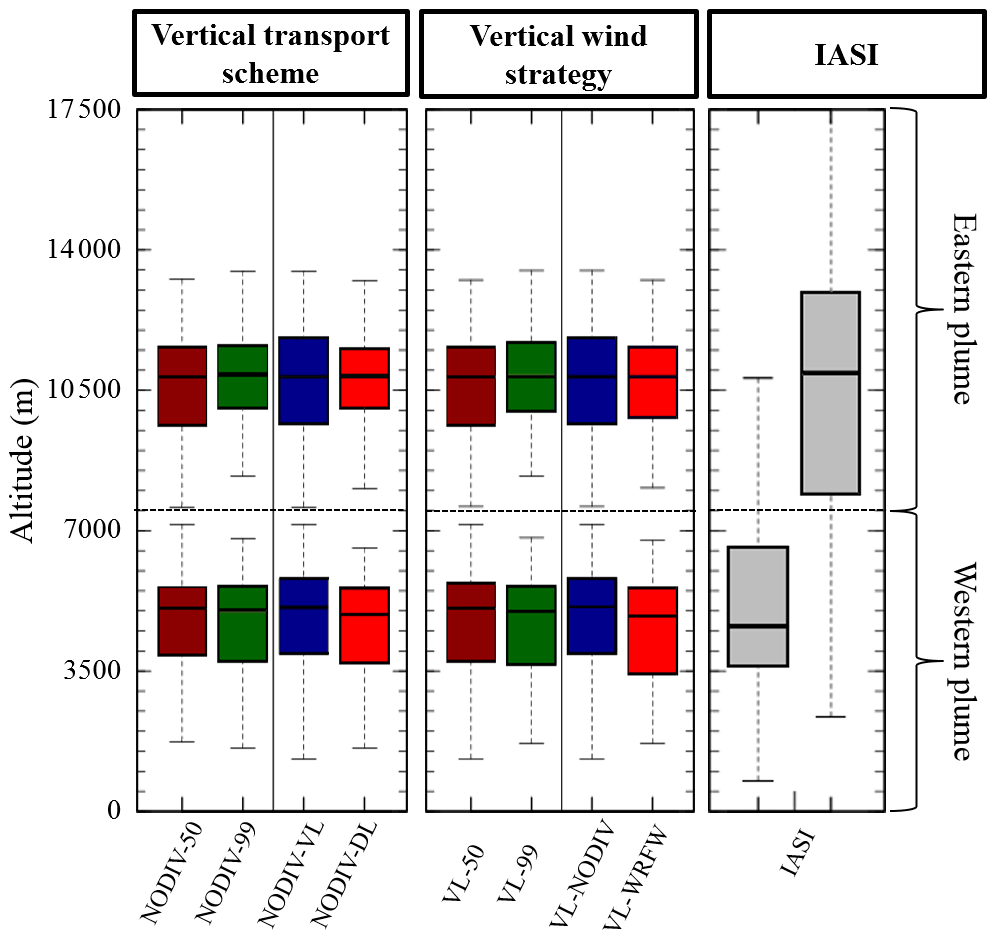
Figure 6 The SO₂ plume maximum concentration's altitude distributions for IASI measurements and CHIMERE model simulations for the different configurations tested. The extents of the whiskers correspond to the distribution's 10th and 90th percentiles.

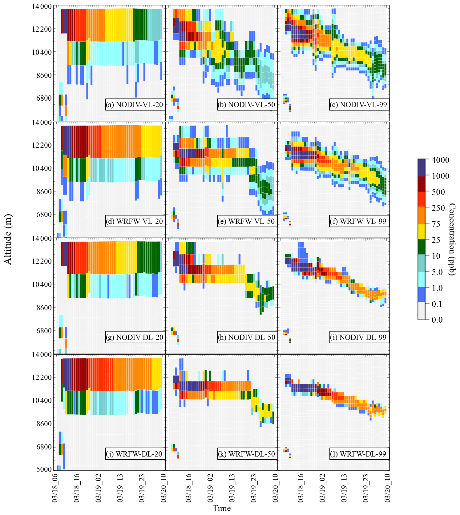
Figure 7 Evolution of the SO₂ vertical profile (in ppb), corresponding to the maximum column for each step after the Mount Etna eruption, for each of the tested model configurations. The top row shows NODIV-VL, the second row shows NODIV-DL, the third row shows WRFW-VL and the fourth row shows WRFW-DL. The left column presents the 20-vertical-level simulations, the center column presents the 50-vertical-level simulations and the right column presents the 99-vertical-level simulations. WRFW simulations values have been corrected to fit NODIV strategy masses.

3.6 Impact of the model configuration on SO₂ vertical diffusion

To directly evaluate the impact of the various model configurations on SO₂ vertical diffusion, the time evolution of the SO₂ vertical profile for the model column with the strongest SO₂ content at each hourly model output steps is shown in Fig. 7. These results display the following:

• 20 vertical levels are clearly insufficient to correctly reproduce even the main features of the plume advection in this case, as no evolution of the plume altitude can be seen at such a coarse vertical resolution, and the plume seems to be strongly leaking through the top of model, which is not the case with 50 or 99 vertical levels.

• WRFW-DL-99 is the simulation that diffuses the plume the least.

• Using an anti-diffusive advection scheme permits the user to reduce diffusion almost as strongly as increasing the number of levels; for example, the NODIV-DL-50 simulation preserves the maximum concentration of SO₂ in the plume and the thin plume structure as well as simulation NODIV-VL-99, with a calculation cost divided by 2 due to the reduced number of vertical levels. Therefore, the use of an anti-diffusive advection scheme is a very attractive means of reducing numerical diffusion in the vertical direction without increasing the computational cost of the simulation.

• Using the realistic WRFW vertical wind instead of the vertically reconstructed NODIV wind also reduces numerical diffusion and avoids intermittent leaks of the tracer through the upper model boundary, as can be seen, for example, by a comparison between the NODIV-VL-20 and WRFW-VL-20 simulations.

• Combining an anti-diffusive advection scheme, the use of real vertical wind and the largest number of levels systematically permits the user to reduce plume diffusion. Qualitatively, the impact of the anti-diffusive transport scheme on reducing vertical diffusion seems to be more pronounced than that of using real vertical winds instead of reconstructed winds: it can be seen from Fig. 7 that plumes in the third row, which use the Després and Lagoutière (1999) scheme and reconstructed vertical winds, are systematically less diffused than their counterparts in the second row, which use the Van Leer (1977) scheme and realistic vertical winds.

• Examination of the four simulations with 99 vertical levels shows that the Després and Lagoutière (1999) scheme preserves much higher maximal concentrations in the plume: at the last simulation step, both simulations using the DL99 scheme exhibit maximum SO₂ concentrations in the 75–250 ppb range, whereas both simulations with the Van Leer (1977) scheme have maximal concentrations in the 10–25 ppb range a little over 48 h after the eruption; thus, all other things being equal, choosing the Després and Lagoutière (1999) anti-diffusive transport scheme allows the simulated concentration to be at least 4 times as strong as with the classical Van Leer (1977) scheme.

3.7 Parameters' impact on SO₂ dispersion

In the aim to evaluate the SO₂ overall diffusion (vertical and horizontal) following the abovementioned Mount Etna eruption, we compared the minimum volume in which 50 % of SO₂ mass can be found for each time step and for each simulation. Volume evolution is represented in Fig. 8a. The 20-level simulations present the highest volume occupied, and the 99-level simulations present the lowest volume occupied. The simulation that restricts diffusion the most is WRFW-DL-99, and the simulation that least efficiently contains the plume is NODIV-VL-20.

To assess the impact of the applied vertical scheme or vertical wind strategy, the volume ratio evolution between the VL and DL vertical scheme for each number of vertical levels has been calculated – with the wind strategy fixed (NODIV). Likewise, the volume ratio evolution between the NODIV and WRFW wind strategy for each vertical levels number was calculated – with the vertical scheme fixed (VL). The volume ratio evolution is summarized in Fig. 8b. It appears that the DL vertical transport scheme strongly reduces diffusion compared with VL, as the volume ratios ${\mathrm{Vol}}_{\mathrm{NODIV}-\mathrm{VL}}/{\mathrm{Vol}}_{\mathrm{NODIV}-\mathrm{DL}}$ increase with time for the three-vertical-level configuration. Results are less clear for the vertical wind strategy, as the volume ratios ${\mathrm{Vol}}_{\mathrm{NODIV}-\mathrm{VL}}/{\mathrm{Vol}}_{\mathrm{WRFW}-\mathrm{VL}}$ slightly increase in most cases, with a stronger effect in the 20-vertical-level case. Finally, we observe that the combination of WRFW and the DL parametrization consequently reduced the atmospheric diffusion, so that the plume volume for WRFW-DL-20 is quite similar to the NODIV-VL-99 case: using a realistic vertical wind field and an anti-diffusive scheme is, for this criterion, as efficient as refining the model vertical resolution by a factor of 5.

As discussed in Zhuang et al. (2018) and Eastham and Jacob (2017), reducing the vertical diffusion has a direct impact on reducing the horizontal diffusion as well. Figure S6 shows integrated SO₂ columns for six model configurations 48 h after the eruption. Here, we can observe that, in terms of maximum value of integrated SO₂ column, WRFW-DL-50 produces a maximum value that is slightly stronger than NODIV-VL-99, with strikingly similar horizontal structures. Moreover, in spite of the fact that 20 vertical layers are clearly not sufficient to reproduce the plume, we can see that, if we take the 99-level simulations as reference points, the output of the WRFW-DL-20 is clearly better than NODIV-VL-20 in terms of horizontal structure and maximal column values, which is visible in many aspects such as the orientation of the low-level plume from southeastern Italy to the Aegean Sea and north–south from the Aegean Sea to eastern Libya as well as stronger maximal values of the SO₂ columns in the main part of the plume above the Middle East. This qualitative comparison is in line with the results of Zhuang et al. (2018) and Eastham and Jacob (2017) in the fact that improving the vertical resolution will also substantially reduce the horizontal spread in the simulated plumes. We also calculated the minimum area containing more than 50 % of the SO₂ mass (Fig. S7), showing that the WRFW-DL simulations concentrate 50 % of the plume mass in an area at least twice as small as their NODIV-VL counterparts.

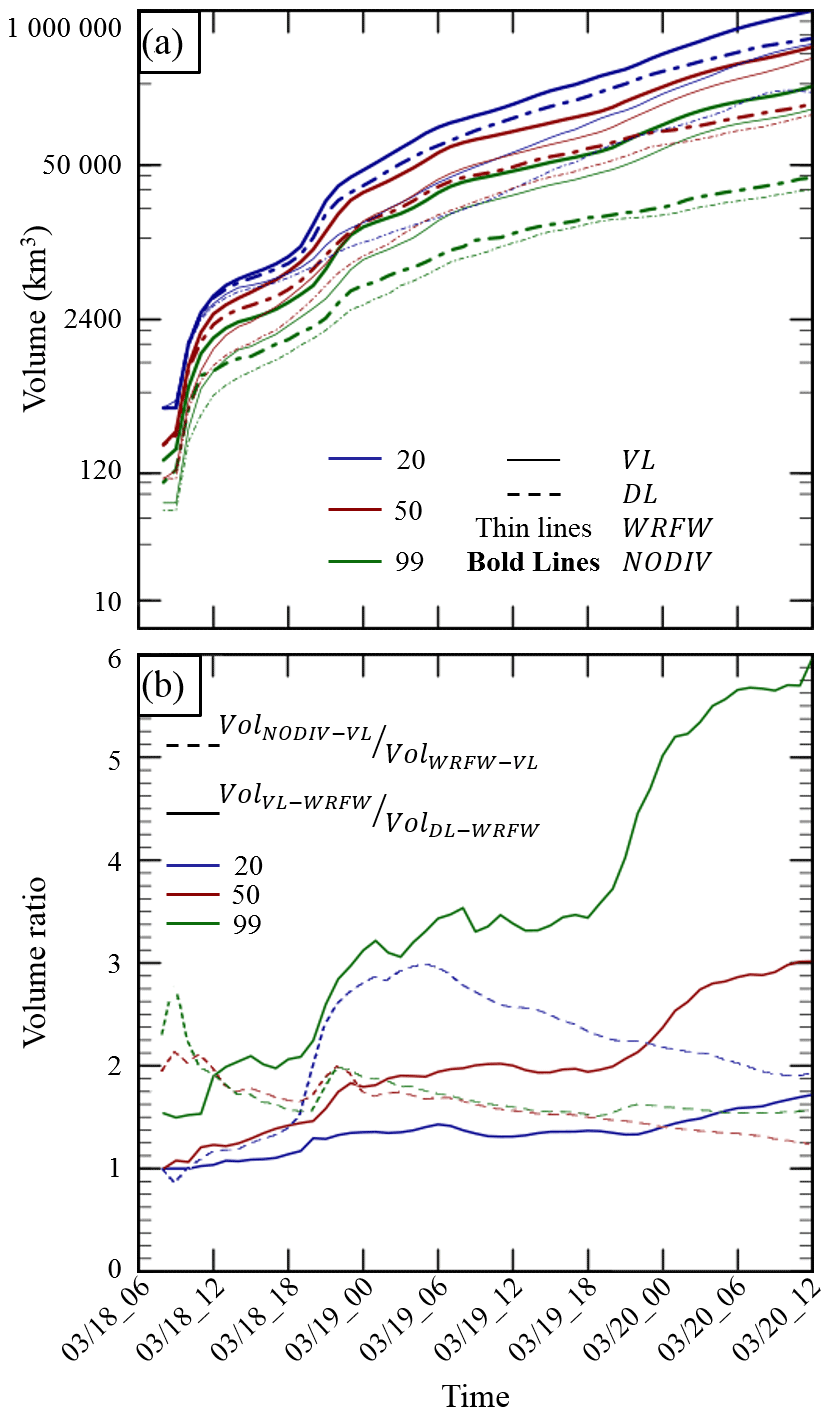
Figure 8 (a) Minimum volume evolution calculated for 50 % of the SO₂ total mass in the atmosphere. (b) Volume ratio evolution by parameters.

4 Conclusion

The Mount Etna eruption on 18 March 2012 was modeled using the CHIMERE chemistry transport model with the aim of proposing and testing strategies to improve the representation of atmospheric vertical diffusion which has previously been described in multiple studies (e.g., Colette et al., 2011; Boichu et al., 2015; Mailler et al., 2017) as over-diffusing, inducing an excessive spread of the simulated plumes. First, the sensitivity to the plume injection height and profile was evaluated by following the plume trajectory with satellite retrievals. In these tests, it appeared that the trajectory is highly sensitive to the injection altitude. The intermediate option (injection at 12 km) was retained, and tests and comparisons were made with this injection altitude. No significant impact of the plume injection profile was observed, and the most simple case of a unique altitude emission was retained.

In order to reduce the excessive spread of the plume in the vertical direction due to numerical diffusion, three possible approaches were tested: increasing the number of levels (20-, 50- and 99-level simulations were performed); using the anti-diffusive scheme of Després and Lagoutière (1999) instead of the classical Van Leer (1977) second-order slope-limited scheme; and using realistic vertical winds instead of vertically reconstructed vertical winds, as it is usually done in CTMs (Emery et al., 2011), at the expense of tracer mass conservation. Our results show that (as expected and as already shown in earlier studies) 20 vertical levels are clearly not sufficient to usefully represent any property of vertical transport or dispersion for this plume and that increasing the number of vertical layers to 50 or 99 provides significant added value in all respects: horizontal trajectories are improved compared with satellite measurements, vertical diffusion is reduced and maximal concentrations are better preserved. The use of the Després and Lagoutière (1999) anti-diffusive transport scheme instead of the Van Leer (1977) scheme is also very effective. To our knowledge, this scheme has never been used in chemistry transport studies, and we show here that this strategy has very strong potential with respect to preventing simulations from being affected by excessive vertical diffusion without dramatically increasing the number of vertical levels. In our simulations, using the Després and Lagoutière (1999) scheme with 50 levels only led to performances that are comparable to those obtained with the Van Leer (1977) scheme and 99 levels (compare Fig. 7c to h or Fig. 7f to k). With an equivalent number of vertical levels, maximum concentrations in the plume after slightly more that 48 h of atmospheric transport are about 4 times as strong in a simulation with the Després and Lagoutière (1999) scheme as in the same simulation with the Van Leer (1977) scheme. In addition, increasing the vertical resolution might give a false appearance of accuracy to the result when the plume injection altitude is not known with good precision. Finally, it has been shown that using realistic vertical winds instead of reconstructed vertical winds also improves the horizontal trajectories of the plume, when compared to satellite observations, and reduces plume diffusion in terms of the minimum volume containing at least half of the plume mass. It needs to be recalled here that this strategy does not guarantee mass tracer conservation. Even though its impact in this respect has been shown to be quite minor in our study, except in the simulations with 20 vertical levels where it generated an initial excess in tracer mass of about 15 %, this characteristic needs to be kept in mind, accounted for and monitored by potential users of this strategy.

These different strategies need to be further studied in different cases to determine whether they can be generalized in CTMs in order to reduce vertical diffusion issues for all pollutants and all kinds of problems, or if they are useful only for the long-distance transport of inert plumes as we simulated here. For example, how does the Després and Lagoutière (1999) scheme perform in preserving smooth gradients, transitions between the PBL and the free troposphere, or gradients in ozone concentrations at the tropopause? Regarding the use of realistic vertical wind fluxes interpolated from meteorological outputs, does it help reduce excessive ozone transport through the tropopause as identified by Emery et al. (2011)? Can this method be generalized to the general chemistry transport modeling of the troposphere in spite of the mass conservation issues that are intrinsic to this method?

This study is a call to reopen the issue of limiting vertical mass diffusion in Eulerian CTMs: complementary to Zhuang et al. (2018), who emphasized the need for sufficient vertical resolution, which is confirmed by the present study, we propose two new approaches to solve this long-standing problem, including anti-diffusive transport schemes and better representation of vertical mass fluxes throughout the troposphere. Our results show that these new approaches to the vertical direction also permit the reduction of horizontal diffusion and that this reduction can be achieved not only by increasing vertical resolution, as shown by these authors, but also by using the Després and Lagoutière (1999) transport scheme as an alternative to classical schemes.