Harmonization of global land use change and management for the period 850–2100 (LUH2) for CMIP6

Human land use activities have resulted in large changes to the biogeochemical and biophysical properties of the Earth's surface, with consequences for climate and other ecosystem services. In the future, land use activities are likely to expand and/or intensify further to meet growing demands for food, fiber, and energy. As part of the World Climate Research Program Coupled Model Intercomparison Project (CMIP6), the international community has developed the next generation of advanced Earth system models (ESMs) to estimate the combined effects of human activities (e.g., land use and fossil fuel emissions) on the carbon–climate system. A new set of historical data based on the History of the Global Environment database (HYDE), and multiple alternative scenarios of the future (2015–2100) from Integrated Assessment Model (IAM) teams, is required as input for these models. With most ESM simulations for CMIP6 now completed, it is important to document the land use patterns used by those simulations. Here we present results from the Land-Use Harmonization 2 (LUH2) project, which smoothly connects updated historical reconstructions of land use with eight new future projections in the format required for ESMs. The harmonization strategy estimates the fractional land use patterns, underlying land use transitions, key agricultural management information, and resulting secondary lands annually, while minimizing the differences between the end of the historical reconstruction and IAM initial conditions and preserving changes depicted by the IAMs in the future. The new approach builds on a similar effort from CMIP5 and is now provided at higher resolution ($\mathrm{0.25}{}^{\circ }\times \mathrm{0.25}$^∘) over a longer time domain (850–2100, with extensions to 2300) with more detail (including multiple crop and pasture types and associated management practices) using more input datasets (including Landsat remote sensing data) and updated algorithms (wood harvest and shifting cultivation); it is assessed via a new diagnostic package. The new LUH2 products contain > 50 times the information content of the datasets used in CMIP5 and are designed to enable new and improved estimates of the combined effects of land use on the global carbon–climate system.

1 Introduction

Over the past several centuries to millennia, human land use activities have grown and intensified to provide food, feed, energy, and fiber to support an expanding human population. These same land use activities have also resulted in large changes to the underlying biogeophysical properties of the Earth's surface, with impacts on climate, biogeochemical cycling, and habitat for biodiversity. In the future, land use activities are likely to expand and/or intensify further to meet future demands for food, feed, energy, and fiber. What have been the effects of land use activities on the climate system? What will be the impacts on climate of future land use scenarios? Addressing these questions requires an integrated set of historical land use data, integrated assessment models of the future, and climate models. To be most useful, requisite land use data must be global in addition to spatially, temporally, and conceptually consistent from the past through to the future and in a format that is usable by Earth system models (ESMs).

Previously, in preparation for the Fifth Assessment Report (AR5) of the Intergovernmental Panel on Climate Change (IPCC) and as part of CMIP5, the Land-Use Harmonization (LUH1) project provided harmonized land use data for the years 1500–2100 at $\mathrm{0.5}{}^{\circ }\times \mathrm{0.5}{}^{\circ }$ resolution (Hurtt et al., 2011). These data served as required land use forcing for CMIP5 climate model experiments and have been used in numerous related studies to assess the effects of land use change on carbon and climate (Brovkin et al., 2013; Jones et al., 2011; Shevliakova et al., 2009, 2013). They have also been extended for use in uncoupled Dynamic Global Vegetation Model (DGVM) modeling studies (e.g., TRENDY, Sitch et al., 2015) and as input to the Global Carbon Project (Le Quéré et al., 2014, 2015a, b) and other studies (Jones et al., 2013; Di Vittorio et al., 2014, 2018; Collins et al., 2015; Arneth et al., 2017; Thornton et al., 2017)

Now, as part of the World Climate Research Program Coupled Model Intercomparison Project (CMIP6; Eyring et al., 2016), the international research community has developed the next generation of advanced ESMs able to estimate the combined effects of human activities (e.g., land use and fossil fuel emissions) on the carbon–climate system. In addition, a set of historical data based on the History of the Global Environment database (HYDE) (Klein Goldewijk et al., 2017), and multiple alternative scenarios of the future (2015–2100), developed by Integrated Assessment Model (IAM) teams (Riahi et al., 2017), including global land use projections (Popp et al., 2017), have been developed as drivers for these models. The goal of the Land-Use Harmonization (LUH2) project is to prepare a new harmonized set of land use scenarios that smoothly connects the historical reconstructions of land use with eight future projections in the format required for ESMs. This ambitious land use harmonization strategy estimates the fractional land use patterns, underlying land use transitions, and key agricultural management information annually for the time period 850–2100 at $\mathrm{0.25}{}^{\circ }\times \mathrm{0.25}{}^{\circ }$ resolution, while minimizing the differences at the transition between the historical reconstruction ending conditions and IAM initial conditions, as well as working to preserve changes depicted by the IAMs in the future to create a consistent set of IAM simulations specifically for this project. The resulting data products are a required input for multiple CMIP6 model experiments, including the historical all-forcing experiment, and related model intercomparison project experiments like PaleoMIP (Junclaus et al., 2017), ScenarioMIP (O'Neill et al., 2016), and LUMIP (Lawrence et al., 2016). Extensions are also provided for 2100–2300 as input to climate stabilization experiments. To bracket the ranges of uncertainty in the historical reconstruction, two alternative scenarios (“low” and “high”) are provided in addition to the “baseline” historical scenario.

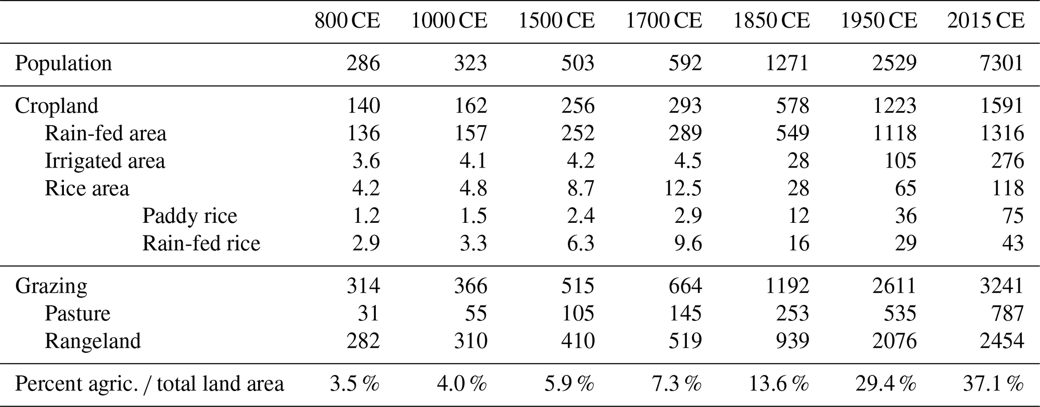
Table 1 Historical global population (millions) and land use estimates (million of hectares) from HYDE 3.2 (Klein Goldewijk et al., 2017).

2 Methods

Like its predecessors, the Global Land-Use Model (Hurtt et al., 2006, 2011), GLM2 (the model underlying the LUH2 dataset), computes subgrid-scale land use states and corresponding transition rates using an accounting-based method that tracks the fractional state of the land surface in each grid cell as a function of the land surface at the previous time step and a transition matrix. This can be represented using the following matrix equation:

$$\begin{array}{}\text{(1)}& \begin{array}{rl}\mathit{l}& (x,t+\mathrm{1})=\mathbf{A}(x,t)\mathit{l}(x,t)\\ & x=(\mathrm{1},\mathrm{\dots },N),t=(t_{\mathrm{0}},\mathrm{\dots },t_f),\end{array}\end{array}$$

where l(x,t) is a vector giving the fractions of grid cell area in each land use category in a grid cell x and time t, and A(x,t) is a matrix giving the land use transition rates between N land use categories in grid cell x and time t. Each element, a_ij(x,t), of the matrix A(x,t) gives the rate at which land use type j was converted to land use type i between t and t+1.

$$\begin{array}{}\text{(2)}& \begin{array}{rl}\mathbf{A}& (x,t)=\left[\begin{array}{ccc}{a}_{\mathrm{11}}(x,t)& \mathrm{\cdots }& a_{\mathrm{1}n}(x,t)\\ \mathrm{⋮}& a_{ij}(x,t)& \mathrm{⋮}\\ a_{n\mathrm{1}}(x,t)& \mathrm{\cdots }& a_{nn}(x,t)\end{array}\right]\\ & (i,j=\mathrm{1}\mathrm{\dots }N)\end{array}\end{array}$$

GLM2 was adapted and extended from GLM1 to track a larger list of 12 subgrid-scale land use types (four “natural land” types, five crop types, two pasture types, and urban) and key management information (i.e., fraction irrigated, fraction flooded, fraction biofuel, and rate of industrial N fertilizer application) related to agriculture. The vector m(x,t) gives the cropland management information for grid cell x at time t, and the state of the full system is therefore described by both the vectors l(x,t) and m(x,t).

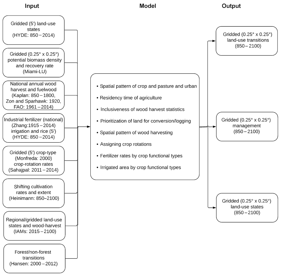
GLM2 was used to solve Eq. (1) and associated values of A(x,t) and m(x,t) annually for every $\mathrm{0.25}{}^{\circ }\times \mathrm{0.25}{}^{\circ }$ terrestrial grid cell globally for 850–2100 (with extensions to 2300). In the process, the framework was used to determine on the order of 10¹⁰ unknowns. Since this was a large and underdetermined system, the approach was to solve the system for every grid cell at each time step by constraining with inputs, including (i) land use maps, (ii) crop type and rotation rates, (iii) shifting cultivation rates, (iv) agriculture management, (v) wood harvest, (vi) forest transitions, and (vii) potential biomass and biomass recovery rates. Because these inputs do not uniquely constrain the system, additional assumptions were made, including (viii) the priority of primary (not harvested, cut, or converted since 850 CE) or secondary land for wood harvesting and agricultural conversion, (ix) the inclusiveness in wood harvest statistics of wood cut in conversion of forest to agricultural use, and (x) the spatial pattern of wood harvest. These model inputs, constraints, and assumptions that are used to compute the state of the system and the associated values of A(x,t) are described in the following sections. The model input–output is illustrated in Fig. 1 and described below.

Figure 1 Schematic diagram of major model inputs, decisions, and outputs.

2.1 Historical maps of land use

Historical maps of land use were based on the History of the Global Environment database (HYDE). HYDE provides long-term historical, spatially explicit time series on a 5 arcmin resolution of population estimates as well as land use reconstructions covering the Holocene period, defined here as 10 000 BCE until the present (Table 1). It is an effort to quantify the agricultural expansion of humankind over time. In principle, HYDE uses a simple approach of combining historical population estimates with assumptions on the trajectory of historical land use per capita. Allocation of land use patterns is steered at the present day by satellite information and UN FAO agricultural land use data (FAO, 2020a), and this is gradually replaced towards the past by a combination of spatially explicit maps such as climate, soil, slope, and neighborhood of rivers and lakes. The latest version (3.2; Klein Goldewijk et al., 2017) presents land use categories such as built-up area, managed pastures and more extensive rangelands, cropland excluding rice, and rice as a separate crop because of its relevancy for greenhouse gas emissions. A distinction was made between irrigated and rain-fed cropland (both for other crops and rice). Besides the baseline reconstruction, two alternative historical land use reconstructions were provided based on uncertainties. For a full description of the methodology, see Klein Goldewijk et al. (2017).

The version of the HYDE 3.2 dataset used for the baseline LUH2 historical product was the 2016_beta_release version, and the version used for the high and low scenarios was the 2017_beta_release_000 version. Data were provided at 5^′ spatial resolution every 100 years from 800 to 1700, every 10 years from 1700 to 2000, and then annually from 2000 to 2015. These data were aggregated to $\mathrm{0.25}{}^{\circ }\times \mathrm{0.25}{}^{\circ }$ resolution and converted from the absolute area of each grid cell to grid cell fractional area. Data were then linearly interpolated in time to produce annual maps of the fraction of each 0.25^∘ grid cell occupied by each of the following land use types: cropland, managed pasture, rangelands, and urban. The ice and water fractions of each grid cell were also taken from the HYDE dataset and were assumed constant over time. By subtracting the land use, ice, and water fractions from each grid cell, the fractions of each grid cell occupied by natural vegetation (either primary or secondary forest or non-forest) were also determined. The HYDE 3.2 dataset also includes a global map that assigns a country code to each terrestrial grid cell at 5^′ resolution. This map served as a basis to generate a similar map at 0.25^∘ resolution, consistent with the 0.25^∘ maps of land use data. In this map every grid cell with an ice ∕ water fraction less than 1.0 was assigned a country code, resulting in a global map containing 199 countries.

2.2 Historical maps of crop types and crop rotations

The cropland fraction of each grid cell, along with transitions to and from cropland, is further subdivided into five different crop functional types (CFTs): C₃ annuals, C₄ annuals, C₃ perennials, C₄ perennials, and C₃ nitrogen fixers. For the years 850 to 2015 the CFT fractions of total cropland are primarily based on data from Monfreda et al. (2008), which provide global maps of harvested areas of 175 different crops at 5 min spatial resolution for the year 2000. For use in the LUH2 methodology, these maps were aggregated into five CFT classes at 0.25^∘ spatial resolution and then normalized so that all CFT fractions sum to 1 in each grid cell. For grid cells that do not have crop-type data from Monfreda et al. (2008), national crop-type data from the FAO (FAO, 2020a) are used instead (i.e., by aggregating the 169 FAO crop types into the five CFT classes represented in LUH, averaging over all years of FAO data from 1961 to 2013, then assigning the normalized national CFT fractions to any grid cells within each country that did not have Monfreda data). The resulting map of CFT fractions is used for all years 850–2015 to subdivide the gridded cropland fraction and cropland-related transitions into CFT fractions and CFT-related transitions by multiplying the cropland fraction of each grid cell (and the cropland-related transitions to and from each grid cell) by the CFT fraction map. Note that this process includes the inherent assumption that the fraction of a grid cell that was harvested for a crop type (i.e., the Monfreda et al. data, 2008) was roughly correlated with the fraction of the total cropland area that was occupied by that crop type.

For the years 2015–2100, we first identify one or two CFTs in the IAM data that have the greatest global area increase over the 85-year period. We then attempt to follow the gridded changes in the fraction of cropland occupied by those CFTs by first assigning as much of the cropland expansion transitions as possible to the expansion of those one or two CFTs and then, when needed, adding transitions between CFTs to reassign area from CFTs with lower rates of increase (or even reductions) of area in the IAM data to the CFTs with large global increases in area. The result of this process is typically that the global area changes of CFTs in LUH2 tend to follow global area changes of CFTs in the IAM data, not just for the CFTs with the largest area changes, but for others as well. When there were no CFTs with significant changes over the 2015–2100 period, the contemporary CFT ratios were used to disaggregate total cropland area into CFT fractions for all years 2015–2100.

Crop rotations, or the practice of growing a sequence of crops on an agricultural field within or across growing seasons, is a key component of agricultural management and has impacts on overall crop yields, nutrient cycling, fertilizer and water usage, water quality, and biodiversity (Bullock, 1992). An example of such a crop rotation is the corn–soybean–corn rotation practiced extensively in the US Midwest. We generated a national-scale crop rotation dataset for the US to quantify rates of transition from one crop functional type to another and applied those rates to the crop functional types in LUH2. We use the USDA Cropland Data Layer (CDL; Sahajpal et al., 2014) to quantify unique crop rotations for the US from 2012 to 2014 (Sahajpal et al., 2014). Assuming a crop rotation span of 3 years and nearly 100 unique crops in the CDL, we could potentially have 10⁶ unique crop rotations. Empirically, there are close to 100 000 unique crop rotations in the US for that time period. However, by aggregating different crop types to the crop functional types in LUH2 and merging similar rotations, we estimated transition rates between different crop functional types in LUH2 and applied them after all other transitions between land use types had been computed.

2.3 Historical data on agriculture management activities

Historical information on crop management activities included data on irrigation, flooded agriculture, and industrial nitrogen fertilizer application rates. Data on irrigated area and area of flooded rice were obtained from HYDE. The irrigated fraction of each crop type was computed during the historical period by dividing the HYDE 3.2 irrigated fraction of each grid cell by the HYDE 3.2 cropland fraction of each grid cell. This fraction is then used as the irrigated fraction of each crop subtype.

The fraction of C₃ annuals flooded for rice is computed in the historical period by dividing the HYDE 3.2 flooded fraction of each grid cell by the C₃ annual fraction of each grid cell (rice is the only C₃ annual considered to be flooded in our dataset; non-flooded rice is not explicitly represented here but would be included in the non-flooded C₃ annual fraction).

For industrial nitrogen fertilizers, we used a recent global compilation of N fertilizer use for 1961–2011 (Zhang et al., 2015) based on FAOSTAT (FAO, 2020b) as our base dataset. Countries without fertilizer data reported in Zhang et al. (2015) were assigned regional mean values based on the regional grouping of countries defined in Zhang et al. (2015). Fertilizer use between 1915 and 1960 was hindcast using global synthetic N fertilizer use totals from Smil (2001) and was forecast from 2012 to 2015 using an estimate of global industrial N fertilizer use based on data from the International Fertilizer Association (IFA, 2015). Decadal mean N fertilizer rates by crop and country were computed from the Zhang et al. (2015) data and were assigned to the mid-decade year (e.g., the 1961–1970 mean was assigned to 1965). To generate country fertilizer application rates for 2015, which we did not compute as a decadal mean, we assumed that the fertilization rate since 2005 has changed with the same scaling factor across all countries and crop types (as in Zhang et al., 2015). Using the harvested area in 2015 from HYDE 3.2 (see Sect. 2.1), the fertilization rate for country j and crop k in 2015 is determined by

$$R_{j,k,\mathrm{2015}}=R_{j,k,\mathrm{2005}}\cdot (F_{\text{2015,IFA}}/A_{\mathrm{2015}})/(F_{\mathrm{2005}}/A_{\mathrm{2005}}),$$

where $R_{j,k,t}$ is the N fertilization rate by crop type (j) for each country (k) by year (t) (kg N ha⁻¹ yr⁻¹), and A_t is the global total crop area in year t from HYDE 3.2; F_2015,IFA is the global N fertilizer application in 2015 estimated by applying the trend in 2006–2012 from the IFA data to extrapolate to 2015 from 2012, yielding F_2015,IFA=115 Tg N yr⁻¹, and F₂₀₀₅ is the global total N fertilizer application estimated as the product of the N fertilizer application rate in 2005 computed from Zhang et al. (2015) and LUH2 cropland area (F₂₀₀₅=94 Tg N, the mean of 2001–2010, as above).

Fertilizer application rates were hindcast from the 1960s to rates for 1950, 1930, and 1915. Synthetic N fertilizer rates in 1915 (and earlier) are set to 0.0 kg N km⁻² for all countries and crop types, as this was when the Haber–Bosch industrial process was invented. Using global N consumption data from Smil (2001) for 1950 (F_1950,Smil=3.7 Tg N yr⁻¹) and 1930 (F_1930,Smil=1.0 Tg N yr⁻¹), as well as crop area from LUH2 ($A_{j,k,t}$, see Sect. 2.1), the synthetic N rates by crop and country ($R_{j,k,t}$) were estimated for 1950, 1930, and 1915 as follows:

$$\begin{array}{rl}& R_{j,k,\mathrm{1950}}=R_{j,k,\mathrm{1965}}\cdot \left(F_{\text{1950,Smil}}\right)/\mathrm{\Sigma }[R_{j,k,\mathrm{1965}}\cdot A_{j,k,\mathrm{1950}}],\\ & R_{j,k,\mathrm{1930}}=R_{j,k,\mathrm{1965}}\cdot \left(F_{\text{1930,Smil}}\right)/\mathrm{\Sigma }[R_{j,k,\mathrm{1965}}\cdot A_{j,k,\mathrm{1930}}],\\ & R_{j,k,\mathrm{1915}}=\mathrm{0},\end{array}$$

where the sum is over all countries (j index) and crops (k index). Finally, we generated annual synthetic N fertilizer rate values by country, crop, functional type, and year ($R_{j,k,t}$) by linearly interpolating between values for 1915, 1930, 1950, 1965, 1975, 1985, 1995, 2005, and 2015.

2.4 Rates of shifting cultivation

We considered shifting cultivation to be a specific land use sequence of clearing, agricultural use typically for 1 to several years, and subsequent abandonment of land to forest (or other natural vegetation) regeneration for 3 years to several decades (“fallow”). While likely widespread in the early millennia of agriculture (Olofsson and Hickler, 2007), more recently it has been restricted to the tropics (Ruthenberg, 1980). We use the recent analysis of the past, present, and future extent of shifting cultivation (Heinimann et al., 2017) to constrain its occurrence in LUH2. Heinimann et al. (2017) based their analysis on the early global map of the distribution of “primitive subsistence agriculture” (Butler, 1980), a visual inspection of the distribution of shifting cultivation based on the 2000–2014 Global Forest Change (GFC) dataset (Hansen et al., 2013) coupled with high-resolution satellite imagery, and an extensive expert survey on regional trends in shifting cultivation, querying lead authors of scientific publications on shifting cultivation over the past decade (Heinimann et al., 2017).

Heinimann et al. (2017) estimated the current area under shifting cultivation (cultivated + fallow) to be about 280 Mha, distributed extensively and heterogeneously across central and tropical South America, tropical Africa, and tropical Southeast Asia (see Fig. 5 in Heinimann et al., 2017). For each $\mathrm{1}{}^{\circ }\times \mathrm{1}{}^{\circ }$ grid cell with detected signs of shifting cultivation, they also estimated its level of occurrence, including both active and fallow cropland, aggregated into five classes of the total land area in each grid cell: none (< 1 %), very low (1 %–9 %), low (10 %–19 %), moderate (20 %–39 %), or high (≥ 40 %). They project significant declines in shifting cultivation extent through the 21st century, with losses by the end of the century of more than 80 % in Africa and Latin America and 100 % in Asia, with extent at $\mathrm{1}{}^{\circ }\times \mathrm{1}{}^{\circ }$ in remaining areas projected to be low or very low (see Fig. 7 in Heinimann et al., 2017).

We created annual LUH2 shifting cultivation maps by linearly interpolating between the assumed shifting cultivation rates in 1850 and the expert-opinion-based rates of 2010 (Heinimann et al., 2017). The 1850 shifting cultivation rates were assumed to fall in the high category of 70 %. The future shifting cultivation rates were similarly computed by linearly interpolating between the 2010 and the assumed 2100 rates from the expert opinion survey of Heinimann et al. (2017). For LUH2, shifting cultivation involved cropland only (grazing land was included as part of shifting cultivation in LUH1 but not in LUH2). For all grid cells, we used the mid-range of shifting cultivation occurrence (e.g., 5 % for “very low”, 15 % for “low”, 30 % for “moderate”, and 70 % for “high”) and assumed that these fractions also applied to the fraction of cropland involved in shifting cultivation. We also assumed that the residence time for a patch of cropland involved in shifting cultivation was only 1 year. At each time step in our model, we then abandoned the Heinimann et al. (2017) prescribed percentage of total cropland area in the grid cell (e.g., cropland to secondary land) and cleared the same area from natural vegetation (e.g., forest to cropland), with a prioritization of clearing secondary land first unless the available secondary land was less than 10 times the cropland area involved in shifting cultivation (based on an assumption of a 10-year fallow period). The global area of shifting cultivation activity tends to track global changes in cropland area from HYDE 3.2 (Klein Goldewijk et al., 2017, or see Sect. 2.1) and global future cropland area changes from IAMs, although this relationship between cropland area and shifting cultivation area declines over time due to the extent of shifting cultivation declining significantly, especially through the 21st century.

2.5 Historical statistics on wood harvest

Historical wood harvest in LUH2 is based on national statistics and partitioned into fuelwood and non-fuelwood for 199 countries based on a 1990 country list from HYDE 3.2 (Klein Goldewijk et al., 2017). These national wood harvest statistics are used to solve Eq. (1) and assigned to individual grid cells using the methodology described in Sect. 2.10 and 2.11. For the years 1961–2015 the LUH2 wood harvest data are based on FAO national wood harvest volume data (FAO, 2020c) for both coniferous and non-coniferous round wood, which is combined with wood density values of 0.225 Mg C m⁻³ for coniferous wood and 0.325 Mg C m⁻³ for non-coniferous wood (Houghton and Hackler, 2000) to convert volume statistics to mass of carbon harvested. Harvest rates were hindcast to 1920 by interpolating from mean FAO per capita harvest rates from 1961 to 1965 using national population totals from HYDE 3.2 (see Sect. 2.1), as well as national per capita fuelwood (“firewood”) and timber (“sawtimber”) wood harvest totals from 1920 (Zon and Sparhawk, 1923). Note that the Zon and Sparhawk totals for timber consumption include volume of wood for construction, industry, and pulp; so, with firewood, it should be roughly comparable to FAO “total roundwood”.

For the years prior to 1920, national annual per capita wood harvest rates were computed in three different ways for low, baseline, and high LUH2 scenarios, and they use the same national population data from HYDE 3.2 to compute the total national wood harvest (Mg C) per year for each scenario. For the low wood harvest scenario, the national annual per capita wood harvest rates from Zon and Sparhawk (1923) were held constant for all years from 850 to 1920. However, prior to the fossil fuel era, global mean per capita wood harvest was likely significantly higher than in 1920, so for the high scenario we used a national per capita wood harvest demand reconstruction for “fuelwood” and “durable wood” from Kaplan et al. (2017) for the period 850–1800. Per capita wood harvest rates then transitioned linearly from 1800 rates to the 1920 rates of Zon and Sparhawk (1923) to mimic the global shift in energy sources from biomass towards fossil fuels (Smil, 2003). These high and low wood harvest scenarios represented two different extremes in terms of cumulative wood harvested and total area of forests removed. In addition, the high scenario is significantly higher than the LUH1 wood harvest reconstruction. To provide a scenario somewhere between these two extremes, we also generated a baseline wood harvest scenario in which we modified the Kaplan national wood harvest rates from 850 to 1800 by national-scale factors. These scale factors are defined as twice the contemporary FAO national per capita wood harvest rates divided by the national per capita wood harvest rates in 1800 from the Kaplan data, and this definition was determined from analysis of the global time series figure of historical biofuel consumption (Smil, 2003), which shows current global per capita biofuel consumption of around 6 GJ per capita and around 21 GJ per capita in 1800. Reducing the Kaplan wood harvest rates via these scale factors does not imply that the original Kaplan rates are too high; rather, the Kaplan data are likely to be capturing types of wood harvest and related processes that our model does not currently simulate. For years between 1800 and 1920 we linearly interpolate between the modified year 1800 rates from Kaplan and the Zon and Sparhawk (1923) rates in 1920.

For the low and baseline scenarios, the reconstructed national wood harvest data were increased by a slash fraction of 30 % (as in LUH1; Hurtt et al., 2011) to account for non-harvested losses from forests that occur during the wood harvesting process. For the high scenario, we do not add a slash fraction to the data for the years 850–1800 since it is assumed this is already included in the Kaplan data (Kaplan et al., 2017). In this scenario, the slash fraction is linearly increased from 0 % to 30 % during 1800 to 1920 and held constant thereafter.

All national wood harvest totals from FAO and Zon and Sparhawk are assumed to represent the amount of wood produced by each country. In contrast, the data from Kaplan represent the wood harvest demand from each country, although it is assumed that during the years 850–1800 there was limited wood trade in most parts of the world, and hence demand would equal production. In Europe, however, international wood trade occurred during 850–1800 (Kaplan et al., 2017). So, for European countries only, if the available national biomass is not sufficient to meet the national wood harvest demand in a particular year, we seek the unmet demand from other European countries (i.e., increase the wood harvest production in other countries) proportional to the available biomass in each country. From 1500 to 2005, the global cumulative total wood harvest in the baseline scenario was 190 Pg C, including slash (Fig. 2), compared with 142 and 381 Pg C in the low and high scenarios, respectively.

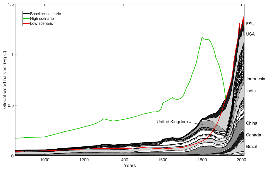
Figure 2 Annual national wood harvest (Pg C yr⁻¹) for 850–2015 for the low, baseline, and high scenarios (FSU: former Soviet Union). Integrated total wood harvest in the baseline scenario was 259 Pg C (including slash).

2.6 Historical maps of forest transitions

The spatial patterns of forest transitions, particularly those related to wood harvesting, were constrained by the Landsat-based gridded forest loss observations from Hansen et al. (2013). This product consists of global 30m grids of tree canopy cover for the year 2000 and gross forest cover loss and gain for the 2000–2012 time interval mapped using the entire global Landsat data archive (although only the forest loss data were used within LUH2). Within this dataset, forest was defined using a single tree canopy cover threshold to match the global forest extent provided by the FAO FRA report (FAO, 2000). Cumulative forest area was estimated by summing pixels with different tree canopy cover. Then the threshold was selected that most closely enabled a match to the total world forest cover for the year 2000, which is 4085 million ha, according to FAO data. A threshold of 28 % tree canopy cover produced 100.5 % of the FAO forest area. This threshold was used to define forest area for the year 2000 at 30 m spatial resolution. Gross forest cover loss was reported only within areas covered with forest in the year 2000. Gross forest cover gain was mapped independently outside areas forested in the year 2000 and represents a gain of tree canopy cover to 30 % or higher from non-forest state. The global maps of forest extent and change were then aggregated to the same spatial resolution and format as the LUH1 datasets ($\mathrm{0.5}{}^{\circ }\times \mathrm{0.5}{}^{\circ }$ fractional). To aggregate the data to the 0.5^∘ grid, the area of each class was computed within each grid cell, and then the class area percent of total cell area was calculated. The 0.5^∘ product shows percent forest cover for the year 2000 and percent gross forest cover loss and gain during the 2000–2012 time interval. The 0.5^∘ product was later downscaled to 0.25^∘ for consistency with the new LUH2 spatial resolution. A very simple downscaling method was employed that kept the fraction of forest area (or forest loss) equal within each 0.25^∘ grid cell inside the 0.5^∘ grid cell.

The resulting map of forest loss was used within LUH2 as part of the algorithm for determining the spatial pattern of forest loss from wood harvesting. However, it should be noted that the Landsat-based forest loss maps differ from the LUH2 forest loss maps in multiple ways, including definitions of “forest” (i.e., tree canopy cover vs. biomass density), whether or not a single grid cell can contain both forest and non-forest (LUH2 grid cells are either potentially forested or potentially non-forested), and whether or not the forest loss includes natural disturbances such as fires (LUH2 forest loss results only from land-use-related changes). As a result, the match between these products is not perfect, and the Landsat-based forest loss data are used as a guide to improve the LUH2 forest loss patterns rather than a hard constraint on those patterns.

2.7 Biomass density and recovery rates

To discriminate forested land from non-forested land and to convert quantities of harvested wood in biomass units into harvested area, information was needed on the historical distribution of forests and aboveground carbon stocks. As no complete global, gridded, historical record of these quantities was available, a simple empirically based global terrestrial model was used to provide a consistent set of both global forest cover and carbon stocks. Estimates of ecosystem properties were based on an updated version of the MIAMI-LU ecosystem model (Hurtt et al., 2002, 2006, 2011). Miami-LU was driven by the empirically based Miami model of net primary production (Leith, 1972), which has integrated sub-models of plant mortality and disturbance. The model tracked subgrid heterogeneity resulting from land use changes in a manner similar to the more advanced Ecosystem Demography (ED) model (Hurtt et al., 1998, 2002; Moorcroft et al., 2001).

Figure 3 Global potential aboveground biomass (AGB; kg C m⁻²) as estimated by the Miami-LU model. Land is considered to be potential forest if the potential biomass density is > 2 kg C m⁻² (after Hurtt et al., 2006, 2011).

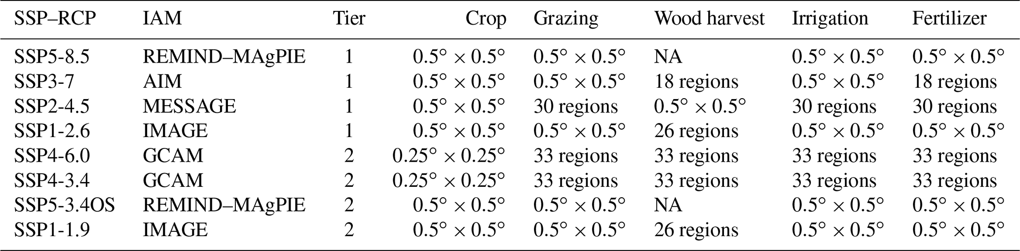
Table 2 Properties of SSPs used in this analysis. SSP and RCP refer to Shared Socioeconomic Pathway and Representative Concentration Pathway, respectively, and Tier refers to the ScenarioMIP Tier (O'Neill et al., 2016).

Miami-LU was run globally at $\mathrm{0.5}{}^{\circ }\times \mathrm{0.5}{}^{\circ }$ resolution for a spin-up period of 500 years using data from the Multi-Scale Synthesis and Terrestrial Model Intercomparison Project (MsTMIP) (Wei et al., 2014). These data are a combination of climatologies from the Climate Research Unit and National Centers for Environmental Protection, and they have a global $\mathrm{0.5}{}^{\circ }\times \mathrm{0.5}{}^{\circ }$ climatology with a 6-hourly daily time step from 1901 to 2010. MIAMI-LU outputs were subsequently downscaled to $\mathrm{0.25}{}^{\circ }\times \mathrm{0.25}{}^{\circ }$ resolution to match the remaining LUH2 inputs (downscaling simply assigned all $\mathrm{0.25}{}^{\circ }\times \mathrm{0.25}{}^{\circ }$ grid cells the same fraction value as the $\mathrm{0.5}{}^{\circ }\times \mathrm{0.5}{}^{\circ }$ grid cell they were contained within). Aggregated globally, the net primary production (NPP) estimate from Miami-LU was 63 Pg C yr⁻¹. This fell within a range of NPP estimates from various global biogeochemical models, ranging from 40 to 81 Pg C yr⁻¹ (Cramer et al., 1999). Miami-LU estimated a global stock of potential plant carbon of 718 Pg C (Fig. 3). This fell within a range spanning 557 Pg C (Kucharik et al., 2000) to 923 Pg C (Sitch et al., 2003), with a more recent estimate of 772 Pg C (Pan et al., 2013). The total potential aboveground carbon stock was 563 Pg C. To differentiate forest from non-forest areas, a definition based on potential aboveground standing stock of 2 kg C m⁻² was used (Hurtt et al., 2002, 2006, 2011). Each grid cell was thus identified as potential forest or potential non-forest based on potential biomass, providing a static map that is used for the entire time period from 850 to 2100. Using this definition, 48.8×10⁶ km² of the land surface was classified as potential forest. For comparison, potential forest area based on the BIOME model was estimated at 60×10⁶ km² (Klein Goldewijk, 2001). Finally, Miami-LU was also used to estimate the recovery of carbon stocks on secondary lands by tracking the mean age of secondary land in each grid cell, although this does not explicitly account for the full age distribution or the potential effects of land degradation, management, or pollution that may have occurred.

2.8 Future land use, wood harvest, and management from integrated assessment models

For 2015–2100, we use land use and wood harvest information from eight different marker SSP–RCP scenarios derived from five different Integrated Assessment Models (Riahi et al., 2017). These marker scenarios were prioritized as input to CMIP6 climate model simulations by ScenarioMIP. They are fully described elsewhere (O'Neill et al., 2016; Riahi et al., 2017), and their main features are summarized below and in Table 2 in the order described in O'Neill et al. (2016).

2.8.1 SSP5-8.5 REMIND–MAgPIE

The scenario SSP5-8.5 is based on the REMIND–MAgPIE SSP5 baseline scenario, which has a radiative forcing close to RCP8.5 (Kriegler et al., 2017). SSP5 is characterized by rapid and resource-intensive development and material-intensive consumption patterns, whereas technological progress, including agricultural productivity, is high. In consequence, the SSP5-RCP8.5 scenario exhibits very high levels of fossil fuel use, up to a doubling of global food demand, and up to a tripling of greenhouse gas (GHG) emissions over the course of the century, marking the upper end of the emission scenario literature. The REMIND–MAgPIE integrated assessment modeling framework consists of the Regionalized Model of Investment and Development (REMIND) and the Model of Agricultural Production and its Impacts on the Environment (MAgPIE). REMIND (Luderer et al., 2015) is a global multiregional energy–economy general equilibrium model linking a macroeconomic growth model with a bottom-up engineering-based energy model. MAgPIE (Popp et al., 2014) is a global multiregional partial equilibrium model of the land use sector, which accounts for spatially explicit biophysical constraints derived by the vegetation, hydrology, and crop growth model LPJmL (Müller and Robertson, 2014; Bondeau et al., 2007; Bodirsky et al., 2012). Land use decisions in MAgPIE are modeled at a spatially explicit level (Lotze-Campen et al., 2008). REMIND and MAgPIE are coupled by exchange of price and quantity information on bioenergy and GHG emissions (Popp et al., 2011; Kriegler et al., 2017). As an outcome of the strongly increasing food and feed demand as well as highly intensified future livestock production systems relying on concentrates rather than roughage feed (Weindl et al., 2017), the SSP5-RCP8.5 scenario shows strong expansion of global cropland into pasture and forest land, with an increase of about 300 Mha (20 %) between 2010 and 2100.

2.8.2 SSP3-7 AIM

SSP3-7.0 is a simulation derived from the SSP3 baseline scenario (Fujimori et al., 2017), which has a radiative forcing close to 7.0 W m⁻². SSP3-7.0 was simulated using the Asia-Pacific Integrated assessment Model/Computable General Equilibrium model (AIM/CGE; Fujimori et al., 2014, 2012) combined with a land use allocation model (Hasegawa et al., 2017). AIM/CGE is a global integrated assessment model coupling representations of economy, energy systems, land, and climate. AIM/CGE is a recursive dynamic general equilibrium model that adjusts prices until the supply and demand for energy, industrial, agriculture, and forest commodities as well as all the other goods and services equilibrate. AIM/CGE includes 17 regions and 42 industrial classifications including 10 agricultural sectors. The land system is divided into nine agroecological zones. Land use and land cover were further downscaled to 0.5×0.5 grids using the land allocation approach developed by Hasegawa et al. (2017). SSP3 is a world of regional rivalry in which countries increasingly focus on domestic and regional issues. Economic development is slow, consumption is material-intensive, and population growth is low in industrialized and high in developing countries. Land use change is hardly regulated. Agricultural land intensification is low, especially due to very limited transfer of new agricultural technologies to developing countries. Unhealthy diets with high animal shares and high food waste prevail. A regionalized world leads to reduced trade flows for agricultural goods. The SSP3-RCP7.0 scenario includes strong expansion of global crop and pasture land, with increases of 40 % and 7 % from 2010 to 2100, respectively, resulting in large-scale deforestation.

2.8.3 SSP2-4.5 MESSAGE

SSP2-4.5 is a low stabilization scenario that stabilizes radiative forcing at 4.5 W m⁻² (∼ 650 ppm CO₂ equivalent) before 2100 without ever exceeding that value. RCP4.5 is simulated in a structure of interlinked disciplinary and sectorial models referred to as the IIASA Integrated Assessment Modelling (IAM) framework (Riahi et al., 2007; Fricko et al., 2017). Within the framework, land use dynamics are modeled with the Global Biosphere Management Model (GLOBIOM), which is a recursive-dynamic partial-equilibrium model (Havlík et al., 2011). GLOBIOM includes a bottom-up representation of the agricultural, forestry, and bioenergy sector, which allows for the inclusion of detailed grid cell information on biophysical constraints and technological costs, as well as a rich set of environmental parameters, including comprehensive AFOLU (agriculture, forestry, and other land use) GHG emission accounts and irrigation water use. For spatially explicit projections of the change in afforestation, deforestation, forest management, and their related CO₂ emissions, GLOBIOM is coupled with the G4M model (Kindermann et al., 2006, 2008; Gusti, 2010). These models are linked to the MESSAGE energy system model (Messner and Strubegger, 1995; Riahi et al., 2012), while air pollution implications are derived with the help of the GAINS model. An important feature of RCP4.5 is the initial decrease in forest by about 43 million ha from 2000 to 2050 (comparable to the reference scenario), with a subsequent increase in forest by about 331 million ha from 2050 to 2100.

2.8.4 SSP1-2.6 IMAGE

The SSP1-2.6 scenario is developed using the IMAGE 3.0 integrated assessment model (Stehfest et al., 2014). IMAGE is a model framework describing the future agriculture system and energy system, as well the changes in future land cover, the carbon and hydrological cycle, and climate change. While most socioeconomic processes are described at the level of 26 regions, environmental processes are modeled on a grid basis (30 or 5 arcmin). The LPJmL model is hard-coupled to IMAGE on a yearly basis (Mueller et al., 2016) and calculates for crop and grassland productivity, natural vegetation dynamics, hydrology, and the carbon cycle. The SSP1-RCP2.6 is derived from the SSP1 baseline scenario, which projects a future under a green growth paradigm (van Vuuren et al., 2017). The SSP1 scenario is characterized by moderate population growth leveling off by mid-century and by high economic growth and technological improvements including agricultural productivity. In addition, SSP1 describes an environmentally aware world concerned with limiting biodiversity loss and reduced appetite for animal product consumption. Mitigation policy is added to the SSP1 baseline scenario to achieve a maximum warming of 2 ^∘C, consistent with the RCP2.6 scenario (van Vuuren et al., 2011). Important policies from the land use perspective are increased bioenergy use in combination with carbon capture and storage, avoided deforestation policy to reduce deforestation, and restoration of degraded forests (Doelman et al., 2018).

In SSP1-2.6, the combination of socioeconomic trends and climate policy results in substantial reductions in total agricultural land. At the same time, large areas are dedicated to bioenergy production, and forest area also increases (Doelman et al., 2018; Popp et al., 2017).

2.8.5 SSP4-6.0 GCAM

SSP4-6.0 is a simulation derived from the SSP4 baseline (Calvin et al., 2017), with a modest climate policy imposed to limit 2100 radiative forcing to 6.0 W m⁻². SSP4-6.0 was simulated using the Global Change Assessment Model (GCAM; Wise et al., 2014). GCAM is a global integrated assessment model coupling representations of energy, water, land, economy, and climate. GCAM is a market-equilibrium model that adjusts prices until the supply and demand for energy, agriculture, and forest commodities equilibrate. GCAM subdivides the world into 32 economic regions. The land system is further subdivided into as many as 18 agroecological zones, resulting in 283 agriculture and land use regions. Land use and land cover were further downscaled to a $\mathrm{0.5}{}^{\circ }\times \mathrm{0.5}{}^{\circ }$ grid using the approach developed by West et al. (2014) and implemented globally in Le Page et al. (2016). SSP4 is a world of inequality, both within and across regions. High-income regions continue to prosper, with increased demand for energy and food. Technological progress, including agricultural productivity, is high. Low-income regions, however, stagnate; increases in total consumption are due to increased population and not increased wealth. Agricultural productivity growth is low. Environmental policies, including reduced deforestation, reforestation, and afforestation programs, are present in high- and medium-income countries only. The SSP4-60 scenario includes modest expansion of global crop and pasture land, with increases of 14 % and 9 % from 2010 to 2100, respectively. The modest climate policy encourages afforestation in the high- and medium-income regions where environmental policies are strong, resulting in a global increase in forest cover of 3 % between 2010 and 2100.

2.8.6 SSP4-3.4 GCAM

The SSP4-3.4 scenario starts from the same baseline as SSP4-60 but includes a more stringent mitigation policy limiting radiative forcing to 3.4 W m⁻² in 2100. SSP4-3.4 was also simulated with GCAM (described above). Limiting 2100 radiative forcing to 3.4 W m⁻² requires a much larger carbon price, exceeding USD 1000 per ton of CO₂ (2005 USD) in 2100, than SSP4-60. This increased carbon price has substantial effects on energy and land use. In particular, ∼ 1200 million ha of land is allocated to the production of bioenergy, resulting in a large increase in total cropland area (80 % increase between 2010 and 2100). Forest cover increases in the high- and medium-income regions as the result of afforestation policies but decreases in the low-income regions as the result of agricultural land expansion. The net effect is that global forest cover increases through mid-century before returning to 2010 levels at the end of the century.

2.8.7 SSP5-3.4OS REMIND–MAgPIE

The SSP5-3.4OS scenario starts from the baseline SSP5-RCP8.5 but includes mitigation policy limiting radiative forcing to 3.4 W m⁻² in 2100. SSP5-RCP3.4OS was also simulated with REMIND–MAgPIE (described above) (Kriegler et al., 2017). This scenario is supposed to follow SSP5-8.5, an unmitigated baseline scenario, through 2040 but includes after 2040 strong mitigation action to rapidly reduce CO₂ emissions to zero around 2070 and to net negative levels thereafter. In consequence, the SSP5-RCP3.4OS pathway shows even stronger cropland expansion compared to the SSP5-RCP8.5 scenario, mainly due large-scale deployment of second-generation bioenergy crops after 2040. Globally, cropland in the SSP5-RCP3.4OS pathway increases by about 800 Mha (50 %) between 2010 and 2100, mainly at the cost of pasture area.

2.8.8 SSP1-1.9 IMAGE

SSP1-1.9 parallels SSP1-2.6 in all aspects but reaches a lower radiative forcing target, namely 1.9 instead of 2.6 W m⁻². Like SSP1-2.6, SSP1-1.9 is also derived from the IMAGE 3.0 integrated assessment model (Stehfest et al., 2014). IMAGE is a model framework describing the future agriculture system and energy system, as well the changes in future land cover, the carbon and hydrological cycle, and climate change, as described above. SSP1-1.9 is based on the SSP1 baseline scenario. As also described above, SSP1 projects a future under a green growth paradigm, with moderate population growth and fast economic growth and technological improvements (van Vuuren et al., 2017). In terms of land use, SSP1 describes a world that is environmentally aware and aims at limiting biodiversity loss and environmental impacts of food consumption. Mitigation policy is added to the SSP1 baseline scenario to limit warming to 1.9 W m⁻² (Rogelj et al., 2018; Doelman et al., 2018). As for SSP1-2.6, important policies from the land use perspective are increased bioenergy use in combination with carbon capture and storage, avoided deforestation policy to reduce deforestation, and restoration of degraded forests (Doelman et al., 2018).

2.9 Harmonization of LUH2 inputs

Harmonization of inputs involved minimizing the difference between the end of the historical reconstruction and the beginning of future projections, as well as preserving as much information on the future from IAMs as possible. Five different IAMs provide future land use, wood harvest, and management data using a variety of variables and units at different spatial and temporal resolutions (Table 2). Prior to harmonization, inconsistencies in definitions, resolutions, and other factors resulted in significant discrepancies. The spread of global cropland values from the IAMs in 2010 was 5 % of the historical reconstruction values in that year, and the spread of global pasture values from the IAMs in 2010 was 23 % of the historical values. Gridded values had even larger discrepancies, differing by as much as 100 % from the historical values. After harmonization, these inconsistencies were eliminated by design of the harmonization methodology. Since some IAMs did not simulate built-up area or urban spread, and for consistency of urban land definitions across all scenarios, the IMAGE model provided land use inputs for built-up area in all scenarios (Doelman et al., 2018). Also, since the REMIND–MAgPIE model did not compute wood harvest amounts, these were provided for the SSP5-8.5 and SSP5-3.4OS scenarios from analogous scenarios computed by GCAM.

The first step in harmonizing inputs was to convert the IAM data into a standardized format for comparison with the historical product. Future land use data were aggregated into the fractions of each grid cell occupied by total cropland, total grazing land (the sum of managed pasture and rangeland), urban land, and natural vegetation (the sum of primary and secondary forest and non-forest) annually at $\mathrm{0.25}{}^{\circ }\times \mathrm{0.25}{}^{\circ }$ resolution. Future data on irrigation and flooded areas were standardized into national totals. Future wood harvest data were standardized into a total national wood harvest demand in megagrams of carbon per year (Mg C yr⁻¹), as was the fuelwood component of that national wood harvest, either by aggregating gridded wood harvest data into national totals or by disaggregating regional wood harvest data using the ratio of national to regional wood harvest from the end of the historical period (i.e., 2015). Wood harvest data that were provided in volume units (m³) were converted to biomass (Mg C) using a conversion factor of 0.2688 Mg C m⁻³. A 30 % slash fraction was added to the wood harvest scenarios. Future fertilizer rates were standardized into national fertilizer application rates in kilograms of nitrogen per hectare per year (kg N ha⁻¹ yr⁻¹) per crop functional type. For future scenarios with only regional data, all countries within a region were assigned the same regional rates. When gridded future fertilizer application rates were available these were also used in LUH2 and were standardized into annual rates per crop type (kg N ha⁻¹ yr⁻¹) at $\mathrm{0.25}{}^{\circ }\times \mathrm{0.25}{}^{\circ }$ resolution. For SSP4-3.4 and SSP4-6.0 (both from GCAM), the fertilizer rates for the GCAM crop types misccrop and palmfruit were used as estimates of fertilizer rates for C₃ perennials, sugarcrop and biomass rates were used as estimates for C₄ perennial rates, oilcrop and misccrop rates were used for C₃ nitrogen-fixing crops, rice and wheat were used for C₃ annuals, and corn was used for C₄ annuals.

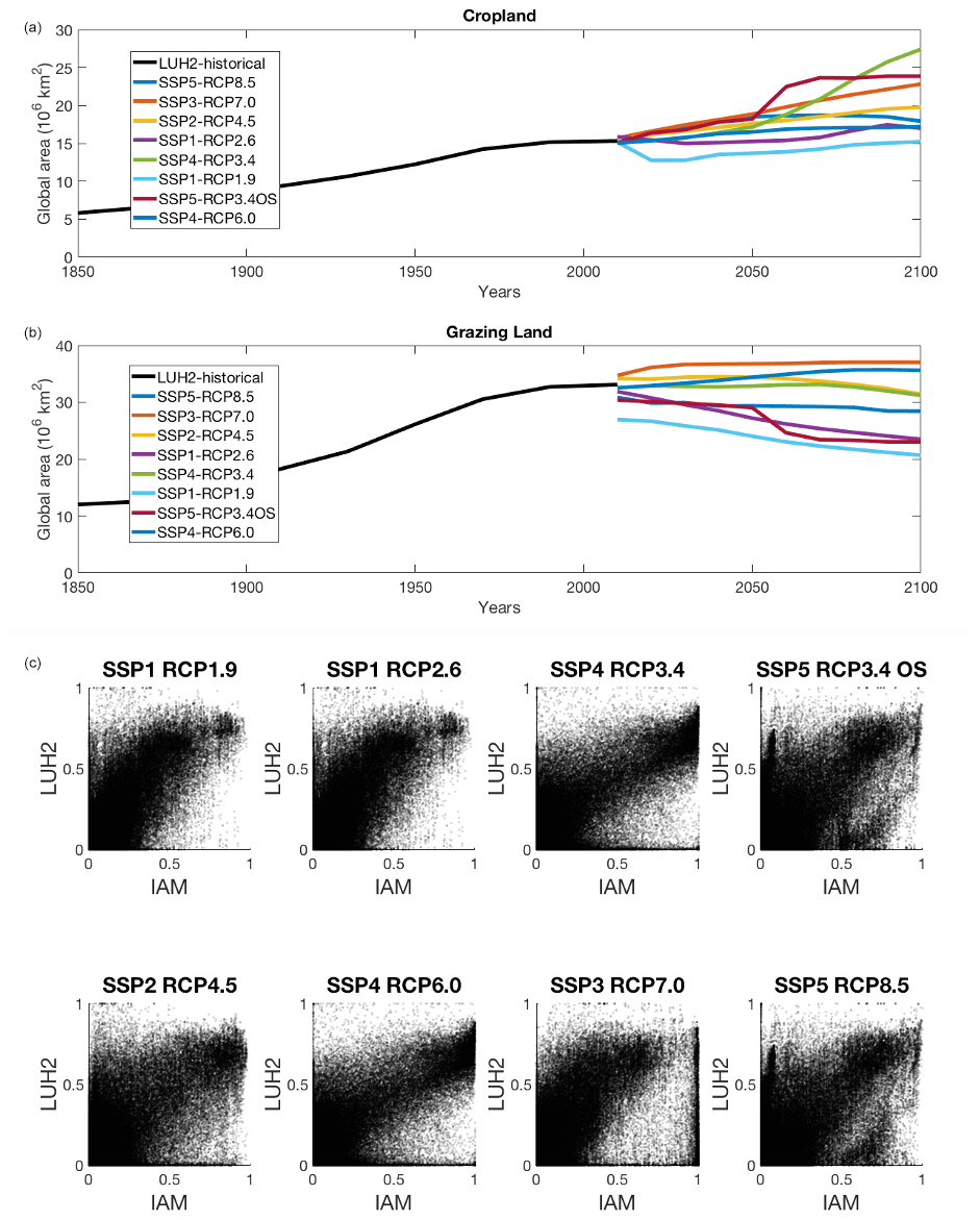
Figure 4 Pre-harmonization (a) global cropland, (b) global grazing land, and (c) 0.25^∘ grid cell comparison of 2015 crop fraction of grid cell areas (excluding water and ice): IAM (x axis), LUH2 (y axis).

Although the IAM land use data were generally in good agreement with end-of-historical-period values at the global scale, there were still significant differences both globally and spatially, particularly for pasture, which has less consistent definitions across models (Fig. 4). To address this issue, we applied IAM-based annual changes in land use sequentially to the spatial pattern of land use at the end of the historical reconstruction. Annual future changes in cropland, grazing land, and urban land were computed and aggregated to $\mathrm{2}{}^{\circ }\times \mathrm{2}{}^{\circ }$. These changes were then applied to the 2^∘ aggregated cropland, grazing land, and urban land from the previous time step, starting with the end of the historical period (i.e., 2015). When it was not possible to apply the annual change within a 2^∘ grid cell due to lack of available land to expand into or lack of cropland, grazing, or urban land to abandon, the unmet changes were applied in neighboring 2^∘ grid cells, starting with immediate neighbors and then radiating outward. The harmonized grids of cropland, grazing land, and urban land were then disaggregated into $\mathrm{0.25}{}^{\circ }\times \mathrm{0.25}{}^{\circ }$ grids according to the following method: when disaggregating decreases, the percentage change in each land use state was computed and then applied to all underlying 0.25^∘ land use fractions; for increases in cropland, grazing, or urban land, the needed change was applied across all underlying 0.25^∘ grid cells and was weighted by available land in each grid cell. Figure 5 shows how well the IAM 2015–2100 changes in cropland and pasture fractions are retained in the harmonized data, which increases markedly with decreased spatial resolution. For wood harvest, analogous methods were applied.

After the harmonization of total cropland, grazing land, and urban land, cropland and grazing areas were further disaggregated into underlying subtypes. Assignment of future crop functional types were based on fixed contemporary Monfreda–FAO proportions and adjusted to match IAM-specific information as needed. For grazing land, a pasture–rangeland mask was generated for 2015 (and held constant for all years) to subdivide future total grazing land into the two grazing subtypes. For new grid cells projected to be converted to grazing land in the future, national ratios were used.

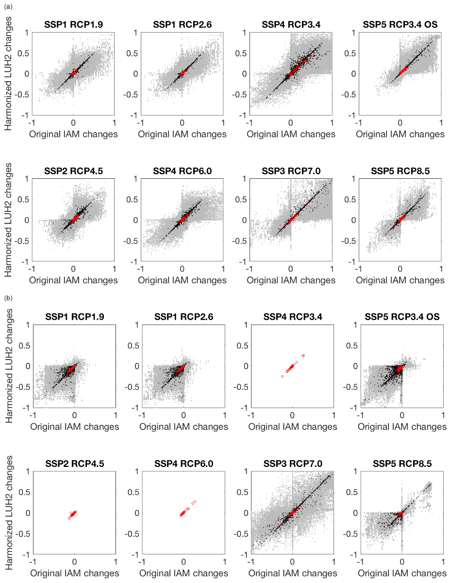
Figure 5 Post-harmonization comparison of projected changes for 2015–2100 at multiple scales: 0.25^∘ (grey), 2^∘ (black), and regional (red) as a fraction of total area. Original IAM change (x axis) and harmonized change (y axis) for (a) cropland and (b) grazing land. Note that for SSP4-RCP3.4, SSP2-RCP4.5, and SSP4-RCP6.0, pasture was only reported by IAMs as regional totals, so LUH2 comparisons at 0.25^∘ and 2^∘ are not possible.

Next, management data were harmonized by applying analogous algorithms to sequentially apply projected changes in managed area and rates to the pattern at the end of the historical reconstruction. Annual changes in national irrigated areas were computed and then applied to the previous year's gridded irrigation fractions for all crop types, first increasing irrigated area on grid cells with existing irrigation, and then adding any additional needed irrigated area equally to all nonirrigated cropland grid cells within each country. Annual national percentage change in flooded area was computed, and this percentage change was applied to all grid cells that have a nonzero flooded fraction in the previous time step. Any resulting fractions that are greater than 1 are reset to 1. Finally, annual national percentage changes in fertilizer rates per crop type are computed. These national percentage changes are applied to the previous year's gridded fertilizer rates for all grid cells within each country. In an effort to ensure that the final (year 2100) gridded fertilizer rates closely approximate the future IAM fertilizer rates, there are a few exceptions to this method, which are based on simple assumptions that aim to keep the LUH2 rates from remaining too low or becoming too large when compared to the IAM gridded rates. First, the gridded fertilizer rates are held between 0 and 500 kg N ha⁻¹ yr⁻¹. Then, for grid cells with fertilizer rates below 1 kg N ha⁻¹ yr⁻¹ in the previous time step and with an increasing national percentage change in fertilizer rates, the actual gridded IAM fertilizer rates for the next time step are used instead of the computed LUH2 rates. Also, if gridded fertilizer rates increase between time steps and are above the gridded IAM fertilizer rates, the gridded fertilizer rates for the next time step are held constant at the current LUH2 gridded rates. Finally, if the gridded LUH2 fertilizer rates are less than 80 % of the IAM gridded fertilizer rates and the national percentage change in fertilizer rates is positive, a small additional increase (1 % of the total current difference between IAM gridded rates and LUH2 gridded rates) is added to the LUH2 fertilizer rates.

2.10 Additional major factors

2.10.1 Inclusiveness of wood harvest

Since it is not always known whether or not the wood cut on land cleared for agriculture is counted in national wood harvest statistics, assumptions are made in LUH2 about the amount of biomass from land clearing that is included towards meeting national wood harvest demands. The need to use wood from cleared land for fuel or wood products was probably higher in the past than it is now. To that end, we assumed that all wood on land cleared for agriculture prior to 1850 was counted towards meeting the national wood harvest estimates and additional wood harvest was only conducted when the land cleared for agriculture did not provide enough wood to meet the estimates. We also assumed that after 1920 none of the wood from cleared land was counted toward meeting national wood harvest numbers and wood harvest demand was met only through explicit wood harvesting activities. Between 1850 and 1920 a fraction of the wood from cleared land was used to meet wood harvest demands, starting from 100 % of wood from cleared lands in 1850 and decreasing linearly to 0 % in 1920. If this fraction of wood from cleared lands was not enough to meet national wood harvest demands, additional explicit wood harvest was conducted to meet national totals.

2.10.2 Priority of land conversion

When converting natural land to agriculture or using it for wood harvest, a decision must be made about whether to prioritize the use of primary or secondary land. The cumulative effect of these decisions has a large impact on the resulting secondary land area, age, and biomass in each grid cell, as well as in aggregate at the regional and global scale. Although the decision of which natural vegetation type to prioritize is undoubtedly variable in space and time, for the sake of simplicity we have chosen a single priority rule for each land use transition type, as follows. For urban expansion, secondary was prioritized. After all secondary land is used, further urban land use demand (if any) was met on primary land. For expansion of cropland and grazing land, both primary and secondary land were used in relative proportion to their availability in each grid cell. For example, if primary land and secondary land occupied 10 % and 90 % of natural vegetation in a grid cell, respectively, then 10 % of the converted natural vegetation would be taken from primary land, and 90 % of the converted natural vegetation land would be taken from secondary land. For shifting cultivation, secondary land was prioritized unless the secondary land area was less than 10 times the cropland area in a grid cell, in which case primary land was prioritized. For wood harvesting, the priority was to take wood from both primary and secondary land in relative proportion to the amount of available biomass in each land type.

2.11 Methodology for calculating land use transitions

2.11.1 Determining agriculture land use transitions

Following Hurtt et al. (2011), a bookkeeping approach was used to calculate annual land use transition rates between five aggregate land use types – cropland, grazing land, urban, primary, and secondary. To determine these, the annual change in urban area in each grid cell was first computed from either the HYDE data (for the historical period) or IAM data (for the future period) and applied proportionally to the cropland, grazing land, and secondary land use categories within the grid cell. If there was not enough land available between cropland, grazing land, and secondary land for a given urban land use increase, the remaining area needed was taken from the primary land within the grid cell. Next, minimum transition rates were calculated between the remaining three land use types (cropland, grazing land, and other; other was defined as the sum of primary and secondary) based on the gridded annual input data on land use patterns from HYDE or the IAMs (adjusted for the transitions into and out of those types associated with urban land use change computed in the previous step). With only three land use types, unique minimum transitions (i.e., solutions to Eq. 1) could be easily determined. Additional transitions associated with shifting cultivation and wood harvest were then determined. In cases of shifting cultivation, land use transitions from cropland to other and other to cropland were both increased by the abandonment rate of agricultural land. Transitions from other were then partitioned into transitions from primary and secondary based on availability and the previously described shifting cultivation algorithm. All transitions from cropland or grazing land to other were defined as transitions to secondary. The amount of wood cut in converting land to agriculture was determined by overlaying these transitions with estimates of biomass density.

After computing transitions between the five aggregate land use types, the transitions to and from both primary and secondary were further subdivided into transitions to and from primary forest, primary non-forest, secondary forest, and secondary non-forest based on the underlying map of potential forest (grid cells with potential biomass density greater than 2 kg C m⁻² were designated as potentially forested). In addition, the transitions to and from grazing land were subdivided into transitions to and from managed pasture and rangeland based on the annual gridded input data from HYDE. The HYDE maps of managed pasture and rangeland for the year 2015 were also used to subdivide grazing land into the underlying grazing subtypes for all years in the future period (2015–2100). Transitions to and from total cropland in each grid cell were further subdivided into transitions to and from each of the five crop functional types (CFTs) using the data and methodology described in the section entitled “Historical maps of crop types and crop rotations”.

2.11.2 Determining area cleared by wood harvest

Since the spatial patterns of wood harvest within each country are not generally known (especially for years outside the period of satellite observations), several assumptions were used to spatially allocate the reconstructed national annual wood harvest demands to individual grid cells within each country and to convert the biomass harvested to an area cleared per grid cell. As a first step, within each country and at each time step, a fraction of the biomass cleared from agricultural land expansion is subtracted from the national wood harvest demand, as described in the preceding section on the inclusiveness of wood harvest data. After wood from agricultural clearing has been subtracted, the remaining national wood demand is then explicitly harvested, first from grid cells with available primary forest and/or mature secondary forest, then from grid cells with young secondary forest, and finally from non-forested land (both primary and secondary). Mature secondary forests are defined using an average probability of harvest vs. biomass function parameterized from detailed age-specific harvesting algorithms previously developed and applied in the US (Hurtt et al., 2002, 2006). Note that since the natural vegetation definitions are based on a mean biomass density, wood harvesting from non-forested land can imply either harvesting vegetation, such as shrubland, that is tree-based albeit with a mean biomass density below that of a forest or harvesting isolated trees within other low-biomass-density vegetation such as grasslands.

Within the group of grid cells containing primary forest and/or mature secondary forest in each country, the first cells to be harvested are all those with a “significant human presence” (SHP), followed by all neighboring cells and radiating outwards, taking only the fraction of biomass needed until the demand has been satisfied or the available biomass exhausted. The use of proximity to an SHP in this algorithm is based on the assumption that proximity to an SHP implies proximity to transportation infrastructure (accessibility) or local markets. Prior to the year 1900, grid cells with an SHP are defined as those grid cells having cropland, managed pasture, secondary land, or urban land area. Grid cells that have Landsat-observed forest loss of at least 10 % of the cell's land area during the period 2000–2012 are gradually included in the definition of SHP between the years 1900 and 2000 until both the land-use-based and Landsat-based definitions of SHP are given equal weighting between 2000 and 2015. The contribution of Landsat-based forest loss to SHP then decreases again between 2015 and 2100.

When harvesting wood from a grid cell chosen using these methods, if only a fraction of the biomass in a grid cell is needed, wood is harvested from both primary forest and secondary mature forest (or from primary non-forest and secondary non-forest) in proportion to their available biomass. Wood harvested from primary land provides an area-based transition of “primary to secondary”, whereas wood harvested from secondary land provides an age (and biomass) resetting–reduction transition of “secondary to secondary”, with the resulting secondary mean age and secondary mean biomass density tracked in the “secma” and “secmb” variables, respectively. To calculate these transitions in area units, the wood harvest biomass was converted using the carbon density of land affected (Hurtt et al., 2006).

In addition to their use in the definition of SHP, the Landsat forest loss data are also used in two additional ways to further constrain the spatial pattern of wood harvesting. First, primary forest and mature secondary forest land that will experience a Landsat-observed forest loss during the period 2000–2012 are protected from wood harvest between the years 1950 and 2000 so that they are available for harvesting during the period 2000–2012. Second, during the years 2000–2012, the Landsat forest loss data are used to constrain the spatial pattern of wood harvest by checking whether the annualized gridded forest loss from the Landsat data has already been met within LUH2. Inclusion of Landsat-based forest loss data in the LUH2 algorithm generates a significant improvement in the match between satellite observations of forest loss and the LUH2 representation of forest loss between the years 2000 and 2012 (Fig. 6).

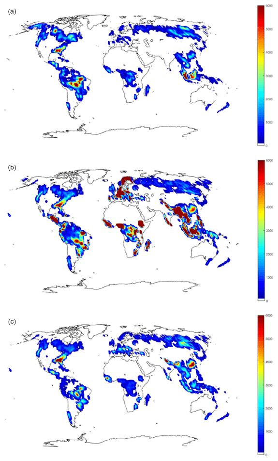
Figure 6 Forest loss 2000–2012: (a) Landsat forest loss (Hansen et al. 2013), (b) LUH2 forest loss without Landsat constraint, and (c) LUH2 forest loss with Landsat constraint.

For European countries that are unable to meet their national wood harvest demand with the available biomass, the unmet wood harvest from each country is reassigned to other European countries (including the former USSR) proportional to available biomass, and the spatial pattern of this additional wood harvest is then allocated using the same rules as outlined above. This is done to model the known trade in wood that was occurring between European countries, even in the early years of our historical simulation (Kaplan et al., 2017).

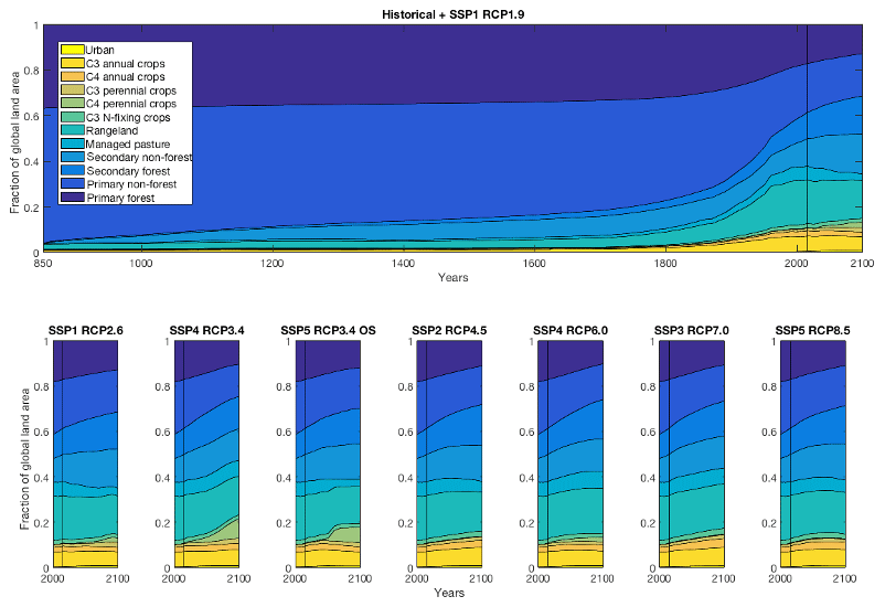
Figure 7 Harmonized global land use area fractions 850–2015 (baseline historical) and 2015–2100 for the eight future scenarios.

2.12 Added tree cover

While it is primarily a land use dataset, LUH2 also provides a simple estimate of forest cover change. For IAM future scenarios with positive forest cover gain (SSP1-2.6, SSP2-4.5, SSP1-1.9), an algorithm was developed to match the spatial pattern of forest gain from IAMs, preserve existing harmonized land use transitions, and be implemented relatively easily in ESMs. For each scenario, a supplementary file was created with a data variable called added_tree_cover. The variable specifies the added tree cover that needs to be planted in each grid cell each year to better represent the corresponding IAM added tree cover estimates. For the other IAM scenarios that are not affected by this issue, added_tree_cover values are set to zero. To produce these datasets, the spatial patterns of differences in forest cover between LUH2 and each corresponding IAM were computed annually for 2015–2100. For each year and each grid cell, if the difference could be met on LUH2 classified non-forest land, that difference was noted as added_tree_cover in the new file. If the gain could not be met on the non-forest area, the change was applied to nearby cells up to four grid cells away.

2.13 Extensions 2100–2300

In addition to the eight future scenarios for the period 2015–2100, the LUH2 dataset also includes extensions for the years 2100–2300 for three of the harmonized future land use forcing datasets for use in long-term climate stabilization experiments. By design, in these extensions, all land use states and management variables are held constant at year 2100 values for the years 2100–2300. As a result, almost all transitions between land use states are set to zero, with the exception of crop rotations and shifting cultivation, which continue at their year 2100 rates, and wood harvest, which uses the year 2099 national wood harvest demands for all years from 2100 to 2299. These extensions to future scenarios are available for SSP1-2.6, SSP5-3.4OS, and SSP5-8.5.

Table 3 Diagnostic table of historical data.

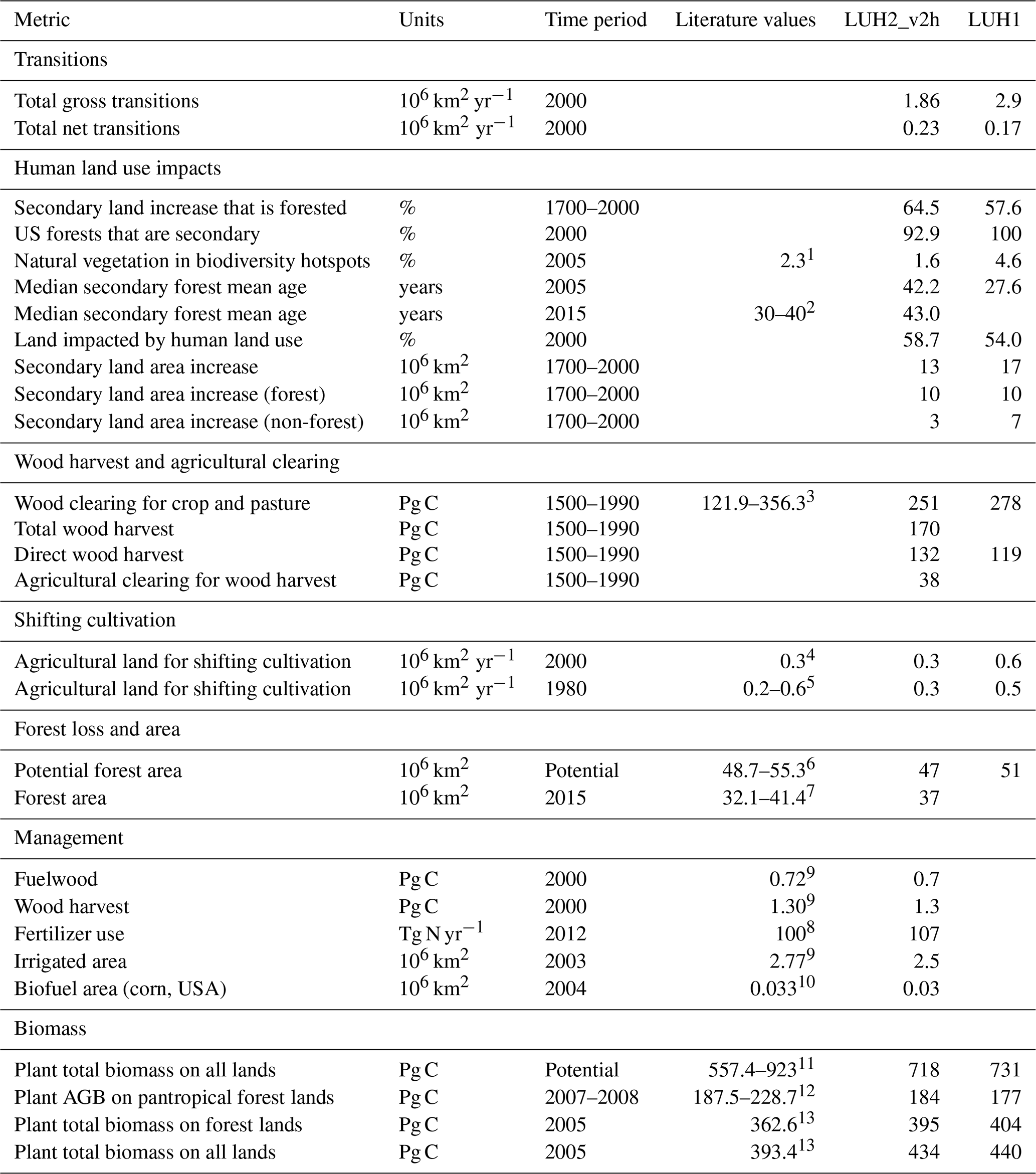
References: ¹ Mittermeier et al. (2005); ² Poulter et al., NACP (2013); ³ Direct wood harvest LUH1, Kaplan low–high case (see text); ⁴ Heinimann et al. (2017); ⁵Rojstaczer et al. (2001); ⁶ Pongratz et al. (2008); Ramankutty and Foley (1999); ⁷ Sexton et al. (2016); ⁸ Zhang (2015); ⁹ FAO (2020c); ¹⁰ Searchinger et al. (2008); ¹¹ Kucharik (2000); Sitch (2003); Pan (2013); ¹² Saatchi et al. (2011); Baccini et al. (2012); Avitabile et al. (2016); ¹³ Pan (2013).

3 Results

3.1 Aggregate results

The annual gridded land use states are aggregated to annual global values by multiplying the grid cell land use fractions by the grid cell area and summing over all grid cells (Fig. 7). The 12 land use states represented in the LUH2 dataset can be further aggregated into the five broader land use categories of total cropland (the sum of all five crop types), total grazing land (the sum of managed pasture and rangeland), primary land (the sum of primary forest and primary non-forest), secondary land (the sum of secondary forest and secondary non-forest), and urban land. Historically, the area of cropland increased at an accelerating rate from 1.7×10⁶ km² in 850 to 4.3×10⁶ km² in 1800 and 15.9×10⁶ km² by 2015 (Fig. 7). Grazing lands increased more rapidly from 3.3×10⁶ km² in 850 to 9.2×10⁶ km² in 1800 and to 32.8×10⁶ km² by 2015. Urban increased from 0 in 850 to 0.6×10⁶ km² by 2015. See also HYDE 3.2 on the historic trends of cropland and pasture (Klein Goldewijk et al., 2017). During the historical period (850–2015 CE), primary land area decreased from 125×10⁶ to 50.1×10⁶ km² (44 % of which is forested), while secondary land increased from 0 to 30.4×10⁶ km² (approximately 49 % of which is forested); note that by definition LUH2 initializes secondary land area to zero in 850 CE. The new land use history reconstruction derived here generally compared favorably to prior reconstructions (Hurtt et al., 2006, 2011) and other references across a range of important diagnostics (Table 3), albeit at higher spatial resolution and with more process detail.

Table 4 Harmonized scenarios of future land use: global land use state areas in the year 2100 across all future scenarios (10⁶ km²).

Table 5 Diagnostic table of future land use.

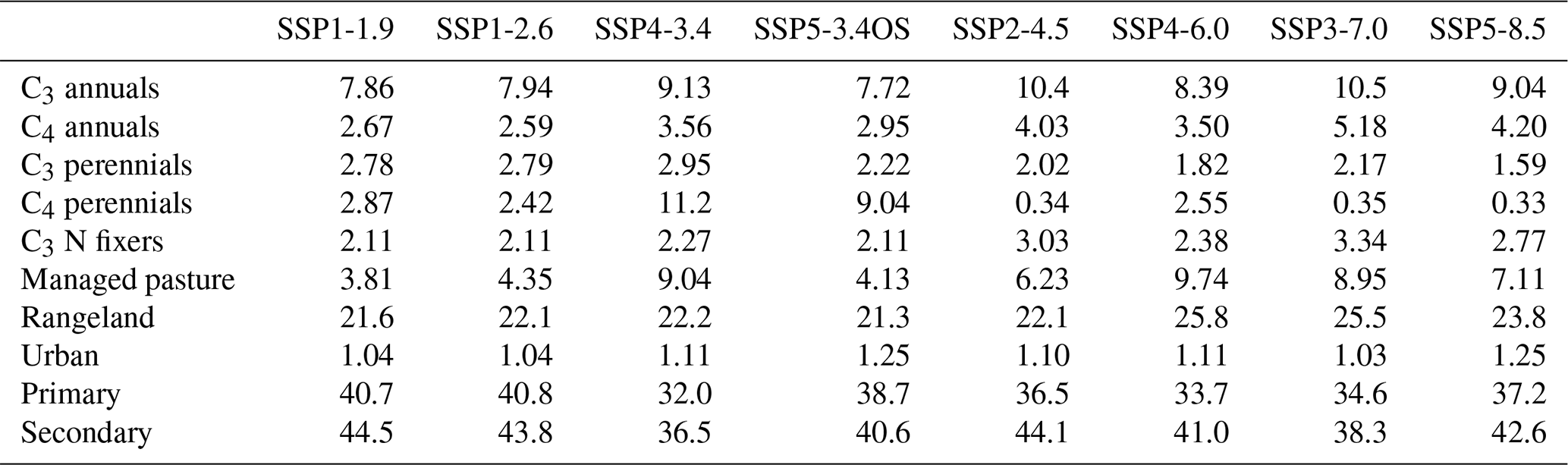
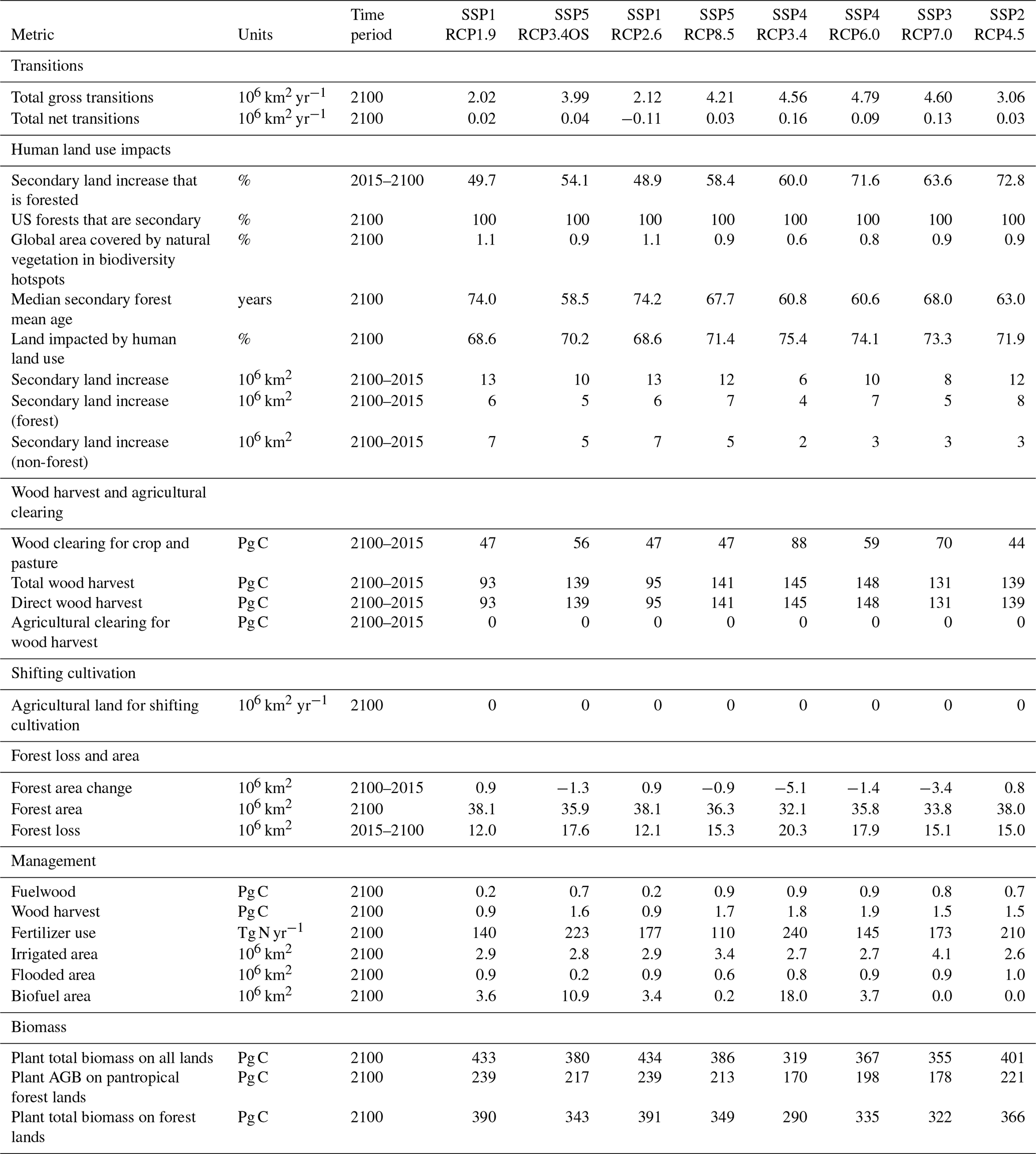
For the future, all eight scenarios projected increases in global cropland area, while six projected grazing land decreases (SSP4-RCP6.0 from GCAM and SSP3-RCP7.0 from AIM projected grazing land increases). The global and regional trends of agriculture and land use in these eight projections are described in detail in Popp et al. (2017), and underlying drivers of these land use dynamics have been identified in Stehfest et al. (2019). For nonagricultural land, six out of eight scenarios projected large increases in wood harvesting, which contributed to large increases in secondary area and corresponding reductions in primary area by 2100. In 2100 global cropland ranged from 17.8×10⁶ km² (SSP1-RCP2.6 from IMAGE) to 29.1×10⁶ km² (SSP4-RCP3.4 from GCAM). As shown in Table 4 and Fig. 15 (panel a), for six out of eight scenarios the dominant crop functional type in 2100 was C₃ annuals, with C₄ perennials (for biofuels) as the dominant crop functional type in 2100 for the remaining two scenarios (SSP4-RCP3.4 from GCAM and SSP5-RCP3.4OS from REMIND–MAgPIE). Global grazing land in 2100 ranged from 25.4×10⁶ to 35.5×10⁶ km², with the majority of that coming from rangeland (Table 4). Secondary land in 2100 ranged from 36.5×10⁶ to 44.5×10⁶ km² (Table 4). In all cases, approximately half of all secondary land was forested, and the estimated mean age of secondary forest ranged from 58 to 74 years. Added tree cover data layers were computed to match the forest tree cover gains of the SSP1-2.6, SSP2-4.5, and SSP1-1.9 scenarios and were able to capture > 80 % of the global afforestation signal in the IAM scenarios. Extensions to the year 2300 were computed for the SSP1-2.6, SSP5-3.4OS, and SSP5-8.5 scenarios and by design did not change the gridded or global cropland, grazing land, or urban land areas. However, due to wood harvesting and shifting cultivation continuing at their end-of-century rates, the area of secondary vegetation continued to grow, and the area of primary vegetation continued to decline in these extensions. By 2300 the global secondary vegetation area in these extension scenarios ranged between 46.3×10⁶ and 51.2×10⁶ km², while the global primary vegetation area ranged between 28.6×10⁶ and 33.0×10⁶ km².

Gross transitions (the sum of the absolute value of all land use transitions) are a measure of all land use change activity. In general, the annual gross transitions tend to increase through time, beginning at 2×10⁵ km² in 850 and increasing to 1.86×10⁶ km² in 2000 (Table 3). The differences between the historical period low, baseline, and high scenarios in LUH2 (computed using three different HYDE land use reconstructions and three different national wood harvest reconstructions) prior to 1920 are primarily due to the differences in rates of wood harvest between those three scenarios. After 1920 the three LUH2 historical scenarios share the same wood harvest reconstruction and their associated gross transitions are very similar. In the future scenarios, gross transitions mostly increased and by 2100 ranged from 2.0×10⁶ to 4.8×10⁶ km² (Table 5).

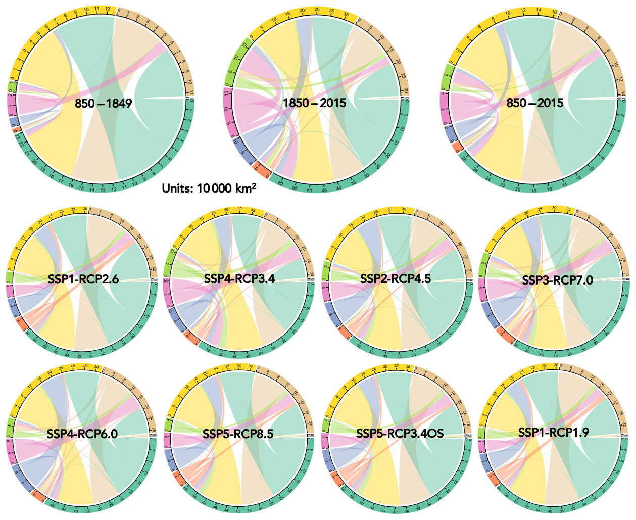
Figure 8 Global land use transitions by time period and by future scenario. Each color represents transitions from a specific land use type to the other land use types: dark green for cropland, orange for managed pasture, blue for primary forest, pink for primary non-forest, light green for rangeland, yellow for secondary forest, brown for secondary non-forest, and grey for urban.

Net transitions measure only the net changes into land use (excluding wood harvest on secondary forests, shifting cultivation, and other agricultural land abandonment that is offset by land conversions to agriculture). Net transitions increase from 2×10⁴ km² in 850 to 2.3×10⁵ km² in 2000 (Table 3). The net transitions across all three historical LUH2 scenarios (low, baseline, and high) are very similar at most time points. The LUH2 historical scenario shows a significant reduction in transitions to pasture around 1950–1960, with implications for carbon investigated separately (Ma et al., 2020). In the future, net transitions range from $-\mathrm{1.1}\times {\mathrm{10}}^{\mathrm{5}}$ to 1.6×10⁵ km² in 2100 (Table 5).

To visualize the magnitudes of transitions between variables, we present chord diagrams indicating the average net transitions occurring annually for 850–1849, 1850–2015, 850–2015, and 2015–2099 for all future scenarios amongst all the major land use categories (Fig. 8). Each arc in a chord diagram represents the average annual area transitioning from one land use to another. The color of the arc represents the land use category from which transition to a different category occurs. For example, in Fig. 8 the arc in light green represents the transition from cropland to other categories. Transitions involving croplands and secondary forest lands dominate land use transitions in all three historical scenarios. The dominant land use transition is secondary forest lands to croplands, and it ranges from nearly 6×10⁴ km² yr⁻¹ in the low historical scenario to 8×10⁴ km² yr⁻¹ in the baseline scenario and 1×10⁵ km² yr⁻¹ in the high scenario when averaged from 850 to 2015. Cropland abandonment activities are also significant, with nearly 1×10⁵, 1.4×10⁵, and 1.7×10⁵ km² of croplands transitioning annually to secondary lands (both forested and non-forested) in the low, baseline, and high LUH2 historical scenarios, respectively (averaged over the entire historical period). On an annual basis, the transitions to and from croplands and secondary lands are generally the same in all three LUH2 historical scenarios.

LUH2 historical results were compared to multiple diagnostics (Table 3). Almost all metrics are within or very close to published reference ranges. These metrics show that 65 % of the secondary land increase between 1700 and 2000 is forested, and 93 % of US forests in the year 2000 are on secondary land. Global natural vegetation in biodiversity hotspots in the year 2005 is estimated as 1.6 % of the land surface (compared with the reference value of 2.3 %). The mean age of secondary land can be calculated for each grid cell and aggregated to a global mean age. For the first several hundred years of the simulation the global mean secondary age grew with time due to primary land being used for land conversion and wood harvesting more often than secondary land (which was initialized to have zero area). Around 1700–1800, existing secondary land was used more often for new land conversions and wood harvesting, and the global mean secondary age started to decrease with time. The median age of secondary forests in the year 2005 is 42 years and is 43 years in the year 2015 (compared with the reference range of 30–40 years). The high scenario had the highest secondary mean age because it had a larger secondary land area, which allows secondary land to be used less frequently for wood harvesting and land conversions. Conversely, the low scenario had a lower secondary mean age than the baseline scenario. The overall land area impacted by human land use in the year 2000 is 59 % of the land surface. The global area of secondary land increase between 1700 and 2000 is estimated as 13.2×10⁶ km², with 10.4×10⁶ km² of that area forested and 2.8×10⁶ km² non-forested.

Cumulative clearing for cropland and pasture between the years 1500 and 1990 resulted in 251 Pg C of wood being removed (compared with a reference range of 121.9 to 356.3 Pg C). Total wood harvest over this period was 170 Pg C, 132 Pg C of which was from direct wood harvest and 38 Pg C was included from agricultural clearing. In the year 2000, an estimated 0.32×10⁶ km² of agricultural land was involved in shifting cultivation (compared with a reference value of 0.3×10⁶ km²). Potential forest area was 47×10⁶ km² compared to a reference value of 52×10⁶ km², and in the year 2015 global forest area was estimated at 37×10⁶ km² compared with a reference range of 32–41×10⁶ km². In the year 2000 global wood harvest was 1.29 Pg C, 0.71 Pg C of which was for fuelwood. Global synthetic fertilizer usage in the year 2012 was 106.6 Tg N yr⁻¹ (compared with a reference value of 100 Pg C), and the global area of irrigated cropland in 2003 was 2.51×10⁶ km² (compared with a reference value of 2.77×10⁶ km²). In 2004, the area of cropland (primarily corn) used for biofuels was 0.03×10⁶ km² compared to the reference value of 0.033×10⁶ km². Total potential plant biomass on all lands was 718 Pg C (compared with a reference range between 557 and 923 Pg C), while total plant biomass in 2005 was 434 Pg C (compared with a reference value of 393 Pg C). Plant aboveground biomass on pantropical forested lands between the years 2007 and 2008 was 184 Pg C (compared with a reference range between 188 and 229 Pg C), and total plant biomass on forested lands in 2005 was 395 (compared with a reference value of 363 Pg C). In addition, the cumulative loss of aboveground biomass resulting from land use transitions (i.e., the sum of all losses) is an important metric of the gross effects of land use on the terrestrial carbon cycle and rose from 0 Pg C in 850 to 5.6×10⁴ Pg C in 2015. Similarly, the cumulative net loss in aboveground biomass is the difference between the estimated aboveground biomass, including land use, and the estimated biomass of potential vegetation; it includes both the losses of aboveground biomass due to land use and the gains due to regrowth. During the historical period the global cumulative net loss of aboveground biomass carbon increases monotonically from nearly zero in 850 to around 310 Pg C in 2015. The low, baseline, and high historical scenarios all give similar global estimates of this metric; the high scenario gives the highest estimates, which is presumably due to the high historical wood harvest in this scenario.

Table 6 Regional results for 1700–2000 (historical period).

In the future scenarios secondary land increases between 6.0 % and 13.27 % across the years 2015 to 2100, with between 48.9 % and 72.8 % of that increase being on potentially forested land (Table 5). The median age of secondary forest in the year 2100 ranges between 58 and 74 years. The global area covered by natural vegetation in the biodiversity hotspots ranges between 0.57 % and 1.08 % of the land surface. Wood clearing for cropland and pastures across the years 2015 to 2100 removes between 44 and 88 Pg C of aboveground biomass, whereas direct wood harvest removes between 93 and 148 Pg C of aboveground biomass. Global wood harvest in the year 2100 ranged between 0.9 and 1.87 Pg C, the fuelwood component of which was between 0.15 and 0.88 Pg C. Total forest area change between 2015 and 2100 ranged from a decrease of 5.1×10⁶ km² to an increase of 3.42×10⁶ km², resulting in a global forest area in 2100 of between 32.1 and 38.1×10⁶ km². Global fertilizer use in the year 2100 ranged between 110 and 240 Tg N yr⁻¹, while the global irrigated area in 2100 ranged between 2.6 and 4.1×10⁶ km². Land flooded for rice in 2100 ranged from 0.23 to 0.96×10⁶ km², and cropland used for growing biofuels in 2100 ranged from 0 to 18×10⁶ km². Total biomass of natural vegetation on forested lands in 2100 ranged between 290 and 391 Pg C, between 170 and 239 Pg C of which is aboveground biomass on pantropical forested lands. In 2100, the global cumulative net loss of aboveground biomass carbon ranges widely across scenarios from 320 to 385 Pg C.

3.2 Spatiotemporal patterns of land use transitions, secondary area, and secondary age

Regional results for the historical period, averaged for each century, are shown in Table 6. In each region or continent, secondary land, gross transitions, and net transitions all tended to increase with time. Secondary land, along with both gross and net transitions, was highest in Eurasia and Africa. Mean regional secondary land area was 8.47×10⁶ km² in Eurasia and 6.01×10⁶ km² in Africa in the 1700s and increased to 12.4×10⁶ km² and 6.82×10⁶ km² in Eurasia and Africa, respectively, in the 1900s. Gross transitions peaked in Eurasia in the 1800s at 660×10⁶ km² yr⁻¹, while net transitions peaked in Eurasia in the 1900s at 121×10⁶ km² yr⁻¹. After 1700, secondary age tended to decrease with time for most regions, although it has held relatively constant over the last 3 centuries for both Africa and Oceania. The range of secondary mean age in the 1900s was between 52 and 289 years. In 1850 there are large areas of cropland in the eastern USA, Europe, India, and China, as well as large areas of primary land worldwide with the exception of Europe, northern Africa, and the Middle East (Fig. 9). By 2015 cropland areas have expanded throughout Africa and the Americas as well, primary land is lost in large areas of the eastern USA, Africa, Europe, India, and China, and the mean secondary age is lower in most locations (Fig. 10).

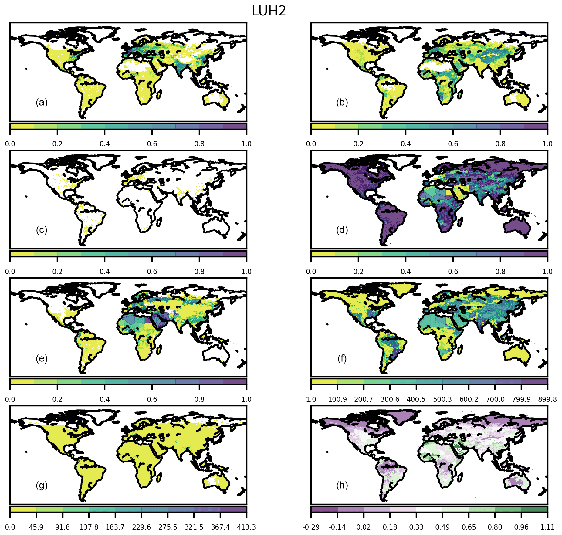
Figure 9 Maps for the year 1850 showing the following: (a) the fraction of each grid cell occupied by cropland; (b) the fraction of each grid cell occupied by pasture; (c) the fraction of each grid cell occupied by urban land; (d) the fraction of each grid cell occupied by primary vegetation; (e) the fraction of each grid cell occupied by secondary vegetation; (f) the mean age (in years) of secondary lands in each half-degree grid cell; (g) the mean gross transitions (km² yr⁻¹) over a 20-year interval for each grid cell; and (h) the mean net transitions (km² yr⁻¹) over a 20-year interval for each grid cell.

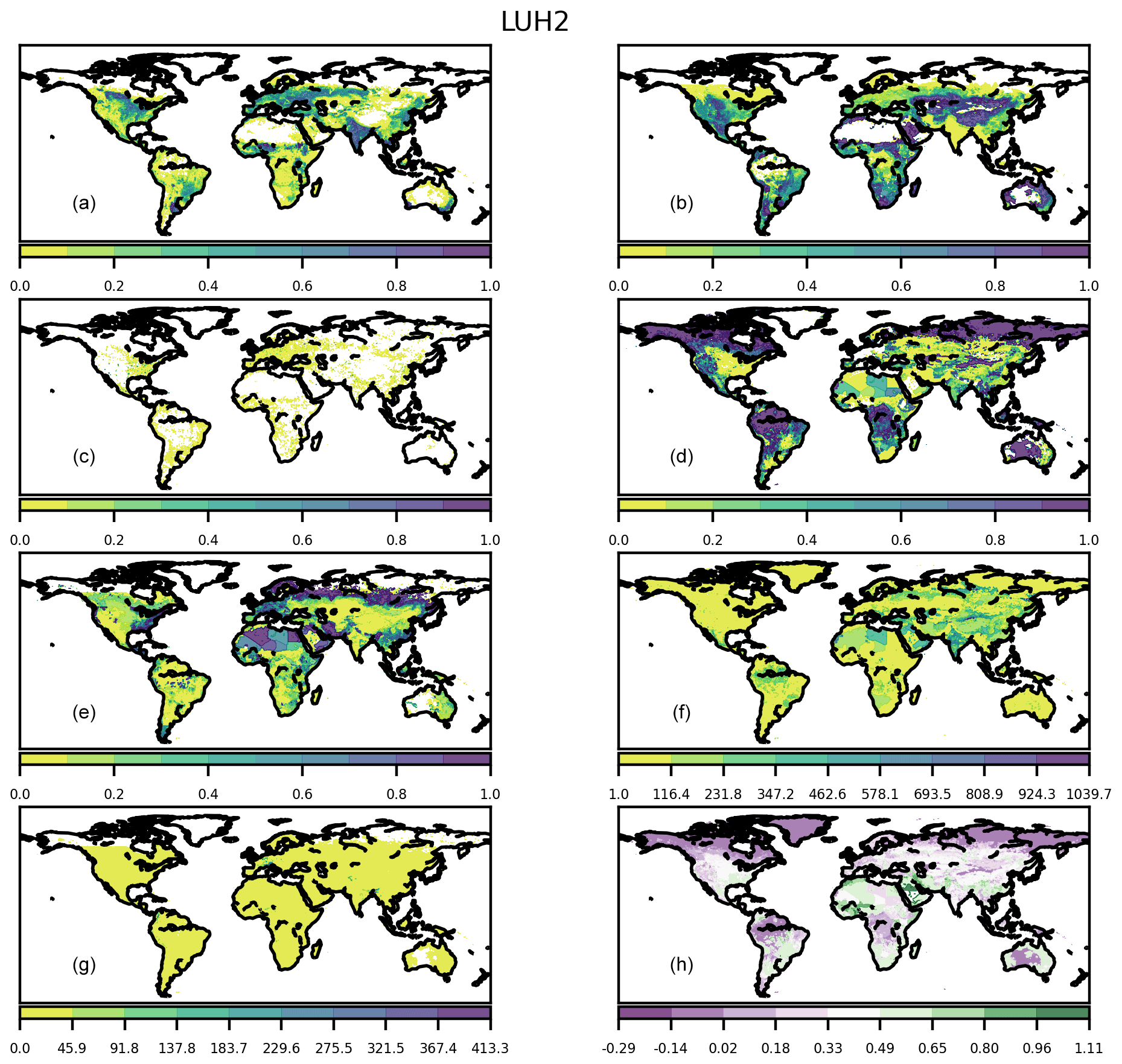
Figure 10 Maps for the year 2015 showing the following: (a) the fraction of each grid cell occupied by cropland; (b) the fraction of each grid cell occupied by pasture; (c) the fraction of each grid cell occupied by urban land; (d) the fraction of each grid cell occupied by primary vegetation; (e) the fraction of each grid cell occupied by secondary vegetation; (f) the mean age (in years) of secondary lands in each half-degree grid cell; (g) the mean gross transitions (km² yr⁻¹) over a 20-year interval for each grid cell; and (h) the mean net transitions (km² yr⁻¹) over a 20-year interval for each grid cell.

Table 7 Regional results averaged over the years 2000–2099.

Regional results are also averaged for the period 2000–2099 for each future scenario (Table 7). Across all scenarios, there were only small differences in regional secondary areas (3.8–4.5×10⁶ km² for North America, 2.0–3.0×10⁶ km² for South America, 17–18×10⁶ km² for Eurasia, 9.2–11×10⁶ km² for Africa, and 0.7–0.87×10⁶ km² for Oceania), with SSP1-1.9 having the highest secondary area on each continent. Secondary land area was highest in Eurasia and Africa for all scenarios. Regional secondary age also did not vary significantly across scenarios; the SSP5-8.5 scenario had the highest secondary age for all regions except Oceania (67 years for North America, 49 years for South America, 209 years for Eurasia, 70 years for Africa, and 50 years for Oceania), and the SSP4-3.4 scenario had the lowest secondary age for most regions (60 years for North America, 45 years for South America, 197 years for Eurasia, 69 years for Africa, and 48 years for Oceania). Secondary age was highest in Eurasia for all scenarios. Gross transitions were highest in Eurasia in seven out of eight scenarios (with Africa the second highest) and highest in Africa in one scenario (with Eurasia the second highest). The highest overall rate of gross transitions was 1936×10⁶ km² yr⁻¹ in Eurasia in the SSP5-3.4OS scenario, but comparable rates of gross transitions were also observed in Eurasia and/or Africa in the SSP4-3.4, SSP4-6.0, SSP3-7.0, and SSP5-8.5 scenarios. Net transitions were largest in Africa in all scenarios (between 34 and 143×10⁶ km² yr⁻¹) and lowest in Oceania in seven out of eight scenarios (and negative in six of those), with South America having the lowest net transitions in the remaining scenario. The SSP4-3.4, SSP4-6.0, and SSP3-7.0 scenarios had the highest rates of net transitions overall at 143×10⁶, 133×10⁶, and 133×10⁶ km² yr⁻¹, respectively.

Large-scale spatial patterns are similar across most scenarios in the year 2100 (Figs. 11–14), with the trends of increased cropland area in South America, continued loss of primary land worldwide and particularly in Africa, and continued reduction of mean secondary age. Analogous mapped results for Tier 2 scenarios are provided in the Appendix.

3.3 Land use management

During the historical period, the use of synthetic nitrogen-based fertilizer on croplands was zero until the early 20th century. After 1950 fertilizer usage started increasing rapidly, and by 2015 global synthetic nitrogen fertilizer usage was 112 Tg N yr⁻¹ (4150 Tg N cumulatively from 1915 to 2015; none prior to 1915), with the majority of this being applied in cropland-dominated locations including North America, Europe, India, China, and Southeast Asia. The eight harmonized future scenarios show a range of potential nitrogen futures; all except one scenario (the SSP5-8.5, which does increase but then falls again to close to current year values) project an increase in global nitrogen fertilizer usage. The range of harmonized global nitrogen fertilizer values in 2100 is between 110 and 240 Tg N yr⁻¹, with the total cumulative use of synthetic nitrogen fertilizer from 2015 to 2100 between 9840 and 14 800 Tg N (Fig. 15b).

Figure 11 Maps for the year 2100 for the SSP5-RCP8.5 scenario showing the following: (a) the fraction of each grid cell occupied by cropland; (b) the fraction of each grid cell occupied by pasture; (c) the fraction of each grid cell occupied by urban land; (d) the fraction of each grid cell occupied by primary vegetation; (e) the fraction of each grid cell occupied by secondary vegetation; (f) the mean age (in years) of secondary lands in each half-degree grid cell; (g) the mean gross transitions (km² yr⁻¹) over a 20-year interval for each grid cell; and (h) the mean net transitions (km² yr⁻¹) over a 20-year interval for each grid cell.

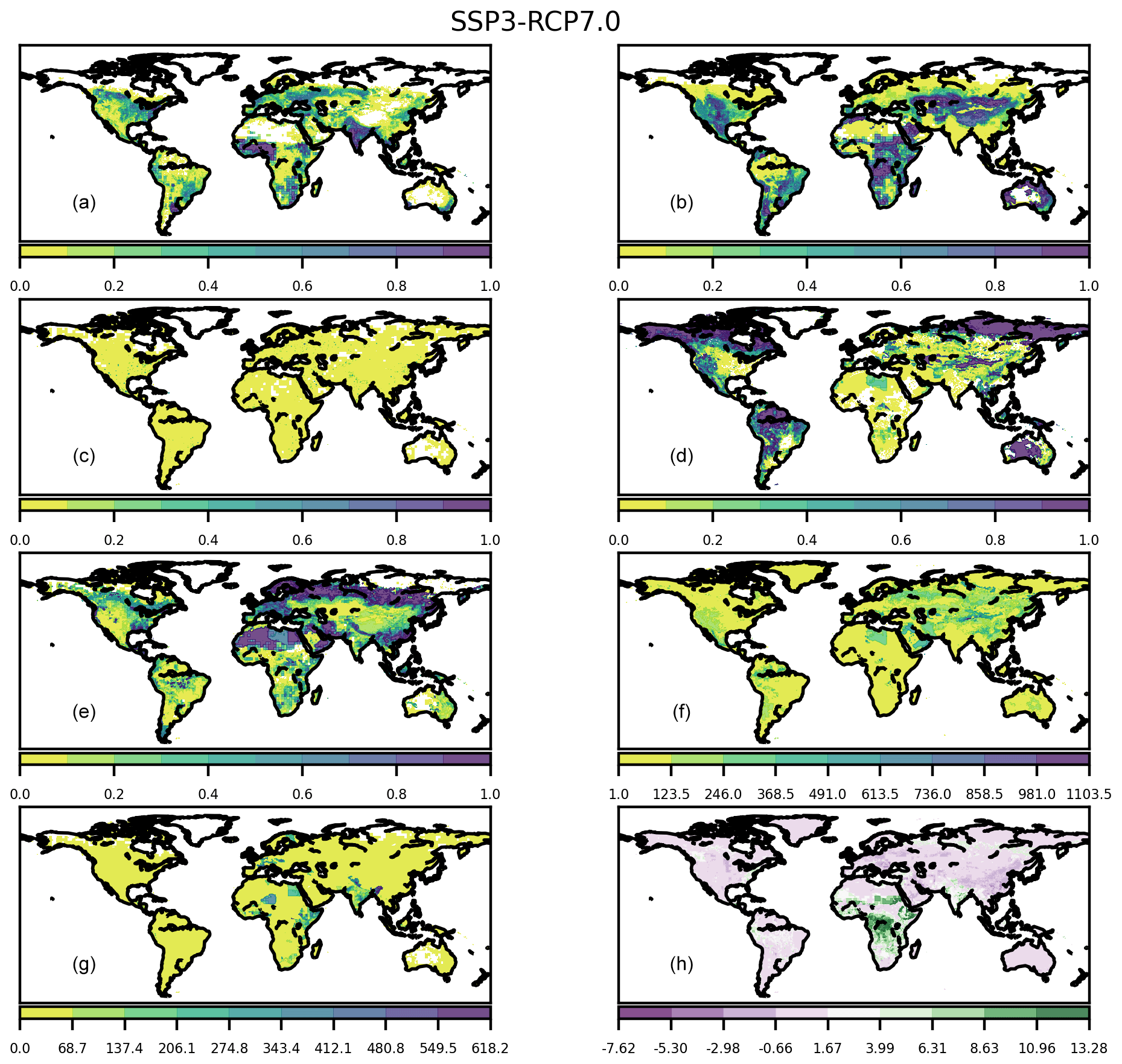
Figure 12 Maps for the year 2100 for the SSP3-RCP7.0 scenario showing the following: (a) the fraction of each grid cell occupied by cropland; (b) the fraction of each grid cell occupied by pasture; (c) the fraction of each grid cell occupied by urban land; (d) the fraction of each grid cell occupied by primary vegetation; (e) the fraction of each grid cell occupied by secondary vegetation; (f) the mean age (in years) of secondary lands in each half-degree grid cell; (g) the mean gross transitions (km² yr⁻¹) over a 20-year interval for each grid cell; and (h) the mean net transitions (km² yr⁻¹) over a 20-year interval for each grid cell.

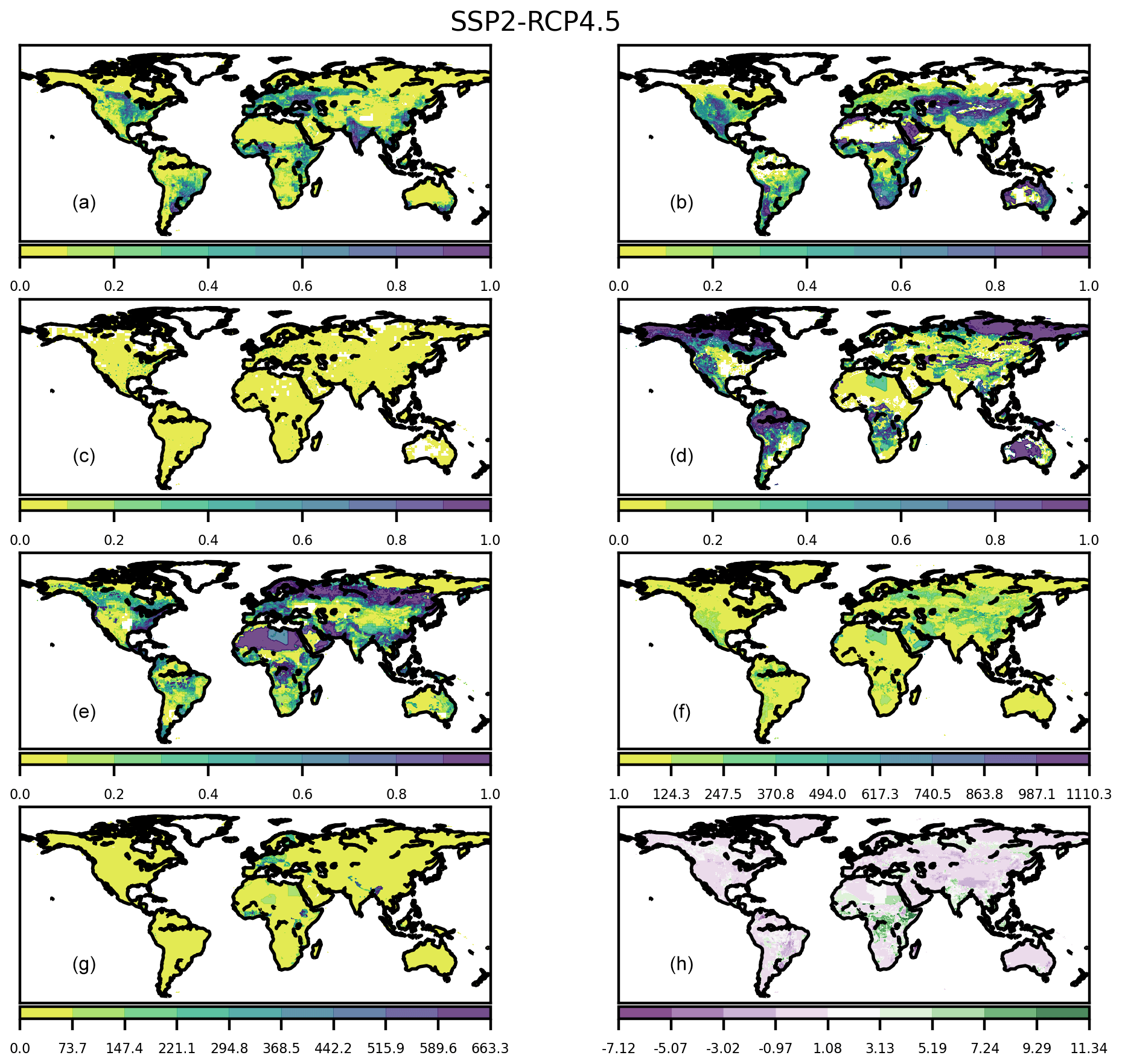
Figure 13 Maps for the year 2100 for the SSP2-RCP4.5 scenario showing the following: (a) the fraction of each grid cell occupied by cropland; (b) the fraction of each grid cell occupied by pasture; (c) the fraction of each grid cell occupied by urban land; (d) the fraction of each grid cell occupied by primary vegetation; (e) the fraction of each grid cell occupied by secondary vegetation; (f) the mean age (in years) of secondary lands in each half-degree grid cell; (g) the mean gross transitions (km² yr⁻¹) over a 20-year interval for each grid cell; and (h) the mean net transitions (km² yr⁻¹) over a 20-year interval for each grid cell.

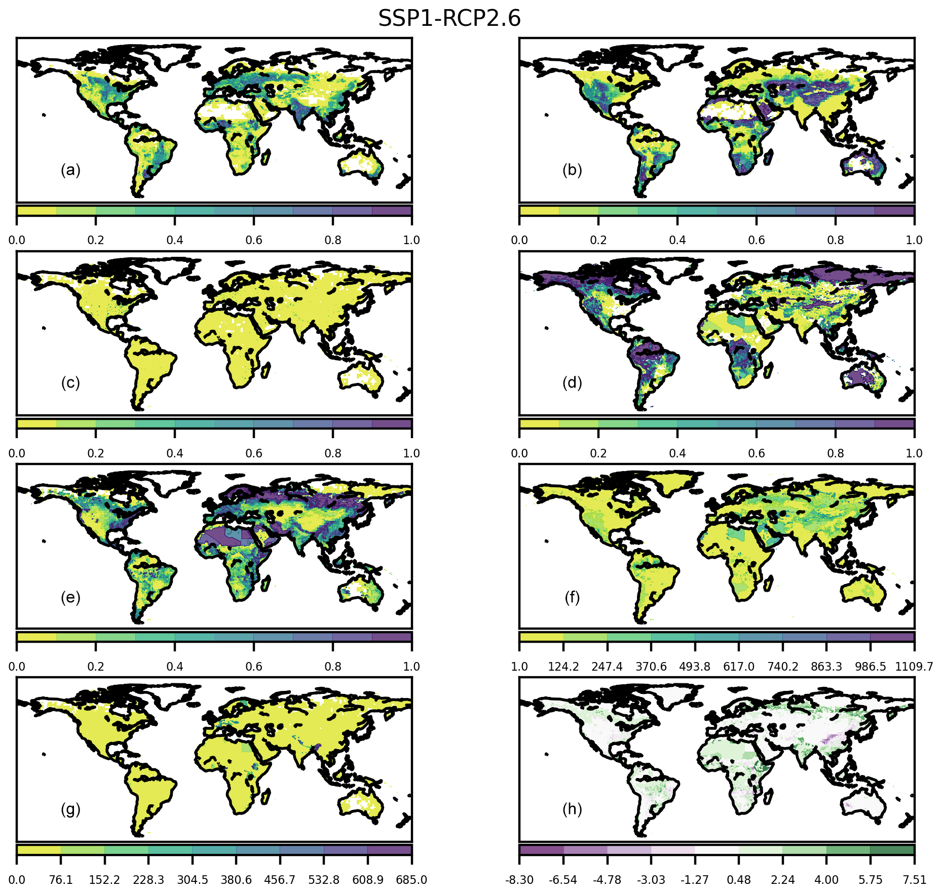
Figure 14 Maps for the year 2100 for the SSP1-RCP2.6 scenario showing the following: (a) the fraction of each grid cell occupied by cropland; (b) the fraction of each grid cell occupied by pasture; (c) the fraction of each grid cell occupied by urban land; (d) the fraction of each grid cell occupied by primary vegetation; (e) the fraction of each grid cell occupied by secondary vegetation; (f) the mean age (in years) of secondary lands in each half-degree grid cell; (g) the mean gross transitions (km² yr⁻¹) over a 20-year interval for each grid cell; and (h) the mean net transitions (km² yr⁻¹) over a 20-year interval for each grid cell.

Figure 15 Time series of harmonized management variables.

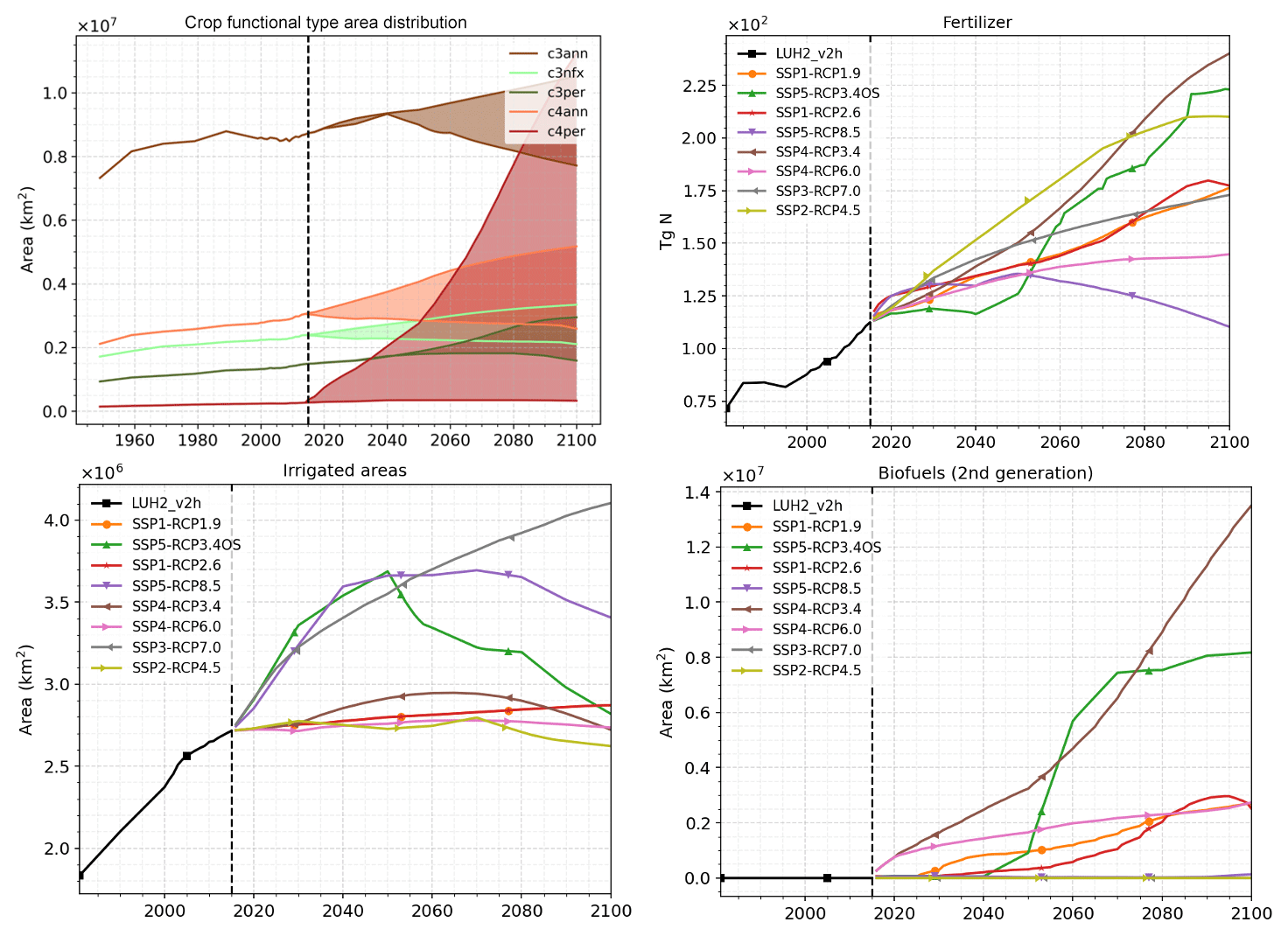
The global area of irrigated cropland increased steadily throughout the historical period and was around 2.7 million km² in 2015. The spatial patterns of this irrigated area show that the majority of global irrigation occurs in India and China, with other significant areas in the USA, Europe, the Middle East, and Southeast Asia. Six out of eight future scenarios project the global irrigated area to remain steady or even decrease slightly, whereas two future scenarios (SSP3-7.0 and SSP5-8.5) show large increases in global irrigated area. The range of values across all future scenarios in 2100 is between 2.6 and 4.1 million km² (Fig. 15c).

The global use of cropland area for purpose-grown biofuels was very low prior to the year 2000 when a small amount of first-generation biofuel production began (such as corn or sugarcane). In the future scenarios the fraction of cropland area grown for first-generation biofuels was held constant, although underlying changes in cropland area resulted in some small increases or decreases in the total area of first-generation biofuels. Second-generation biofuel area (such as miscanthus or switchgrass) expanded in each of the future scenarios, assumed to start from zero in 2015. Five of the eight scenarios (SSP1-1.9, SSP1-2.6, SSP4-3.4, SSP5-3.4OS, and SSP4-6.0) all showed significant increases in the area of second-generation biofuels, while the remaining three scenarios have very little growth in this land management type. By the year 2100, global areas of biofuel crops ranged between 0 and 18 million km², and maps of the spatial distribution of total biofuel area (both first- and second-generation biofuels) show the dominant locations to be the USA, Europe, China, non-Amazonian Brazil, and Argentina. Large expansion of secondary biofuels primarily occurred in Southeast Asia, eastern Europe, the former USSR, and the Middle East (Fig. 15d).

4 Discussion

Land use is essential for meeting human needs for food, fuel, fiber, and shelter, but it also affects the biogeochemistry, biogeophysics, biodiversity, and climate of the Earth. Quantitatively understanding the effects of land use activities on the Earth system requires that the best information on land use be incorporated into the best Earth system models. The strategy described here (LUH2) builds on the approach for harmonizing land use patterns and transitions in CMIP5 (LUH1; Hurtt et al., 2011). This new version is completely updated with new inputs and includes higher spatial resolution (0.25^∘ vs. 0.5^∘), increased detail (12 states vs. 5 and all associated transitions), added management layers, new future scenarios (8 vs. 4), and a longer time domain (850–2100 vs. 1500–2100) – in all more than a 50-fold increase in data from its predecessor. As such, it is designed to facilitate more complete and more consistent treatments of how land use changes influence the Earth system in the past, present, and future.

In comparison to LUH1 (Hurtt et al., 2011), the LUH2 land use history is spatially, temporally, and thematically richer than the previous reconstruction. While not strictly comparable for these reasons, comparing the two products to each other and across a wide range of diagnostics reveals some important quantitative similarities and differences. Historically, the globally aggregated magnitudes of key land use states (i.e., cropland, grazing area) and key land cover variables (forest area and biomass) are generally quite similar (< 10 % difference) over periods of overlap. Larger differences between these datasets are found in the transitions, resulting secondary lands, and spatial patterns of land use activities: contemporary global gross transitions are reduced by ∼ 35 %, contemporary net transitions increased by ∼ 35 %, and estimated primary forest in biodiversity hotspots much closer to independent estimates relative to LUH1 (Jantz et al., 2015). Considering the past, LUH2 begins in 850 CE, 650 years earlier that LUH1. Considering the future, the set of eight future scenarios included in LUH2 doubles that of LUH1, expanding the range of land use forcing that can be considered and including additional cases. Like LUH1, LUH2 also includes extensions to 2100–2300 with no net change in forcing over the interval. LUH2 also includes new added tree cover data to better reflect the changes in tree cover projected by IAMs in afforestation scenarios.

Since management was a new input in LUH2, we do not have comparable values from LUH1. However, the estimates from LUH2 for key management variables are close to empirical estimates and reflect major alterations of nutrient and water cycles, with implications for climate. For example, the ∼ 100 Tg N yr⁻¹ of industrial fertilizer use and irrigated area of ∼ 2.5 million km² by 2000 indicate major human impacts on the functioning of agroecosystems in addition to a general land cover change metric. The inclusion of these activities here as part of the global harmonized dataset is intended to facilitate their inclusion in future global climate assessments, harmonized and together with other concurring land use changes.

These LUH2 datasets are part of the official CMIP6 input4MIPs data collection and are required forcing datasets for Diagnostic, Evaluation, and Clarification of Klima (DECK) and historical climate simulations (Meehl et al., 2014; Eyring et al., 2016). The data are also required for several of the CMIP6-MIP experiments including ScenarioMIP (O'Neill et al., 2016), LUMIP (Lawrence et al., 2016), PMIP (Junclaus et al., 2017), and others. ScenarioMIP defined the set of future scenarios for consideration and organized the official climate–model experiment to quantify the effects of future scenarios of anthropogenic forcing on climate. LUMIP organized the set of model experiments focused on quantifying the effect of land use forcing per se on climate. PMIP is organized to study the historical climate. The central use of these data in the DECK and across a range of important MIPs enhances consistency across CMIP6.

These datasets have also been adopted as required forcing for a range of other international studies including ISIMIP (Frieler et al., 2017), the Global Carbon Project (Le Quéré et al., 2016, 2018a, b; Friedlingstein et al., 2019), and IPBES (Kim et al. 2018). The LUH2 datasets are regularly employed by the TRENDY modeling group in the annual carbon budget estimates of the Global Carbon Project using a simple linear interpolation to update to the year of current budget (Le Quéré et al., 2016, 2018a, b; Friedlingstein et al., 2019). The Global Carbon Project also provides a comparison of land use and land use change emissions with quasi-independent data from two “bookkeeping” models, one of which uses FAO statistics directly and the other uses the LUH2 data. The bookkeeping and process-based model estimates of emissions tend to show high agreement, although in the last 3 years they have begun to diverge (Friedlingstein et al., 2019). This standardization of land use forcing across the breadth of CMIP6 studies and other international assessments has the promise to facilitate maximum consistency in the treatment of land use across the range of interdisciplinary foci and spatial–temporal domains of studies.

Application of the LUH2 data in ESMs, LSMs, DGVMs, and biodiversity models depends on the model type for various aspects. For models with their own vegetation cover different from LUH2, the conversion of forest and non-forest vegetation to agriculture needs to be handled. For conversion into grazing land, managed pasture should always trigger the removal of natural vegetation, while rangeland should only trigger the removal of natural vegetation in forested areas (Ma et al., 2020). A general discussion of transition and conversion challenges in the various models has been described in Prestele et al. (2017).

LUH2 preserves the land use patterns of HYDE 3.2. For gridded land use, HYDE 3.2 took into account the ESA-CCI land cover products (Klein Goldewijk et al., 2017). However, on a national scale, HYDE 3.2 is consistent with FAO land use data (FAO, 2020a) and other statistical databases; differences to satellite-based land cover products cannot be avoided and can be large (Li et al., 2019).

The LUH2 dataset was developed to provide globally consistent and coherent gridded land use for more than a millennium, spanning the past and future, as a necessary input for Earth system model simulations for CMIP6. The requirement of global consistency through time means that it did not always incorporate all of the best local, regional, or national historical data available. For this reason, it may not necessarily be the optimal dataset for a local or regional analysis of land use impacts on biogeochemistry or biodiversity.

Looking ahead, ongoing CMIP6 and several other international activities will be engaged in using LUH2 data as input to studies of global climate, carbon, biodiversity, and other assessments. These data products are intended to meet current needs of models and also provide new variables that most models do not yet include but that may be important. Examples of these features include transitions, introduced in LUH1 and now a growing feature of many models, and now management variables. Model development will need to continue to advance to utilize these features. Meanwhile, advances need to proceed for the next generation of land use harmonization, which should build on these advances and include additional data constraints, more process detail, and a focus on reducing uncertainty of the most sensitive features. This should be part of a larger effort to develop a robust process to provide the best forcing datasets for future global assessments.

Appendix A: Mapped patterns of Tier 2 scenarios

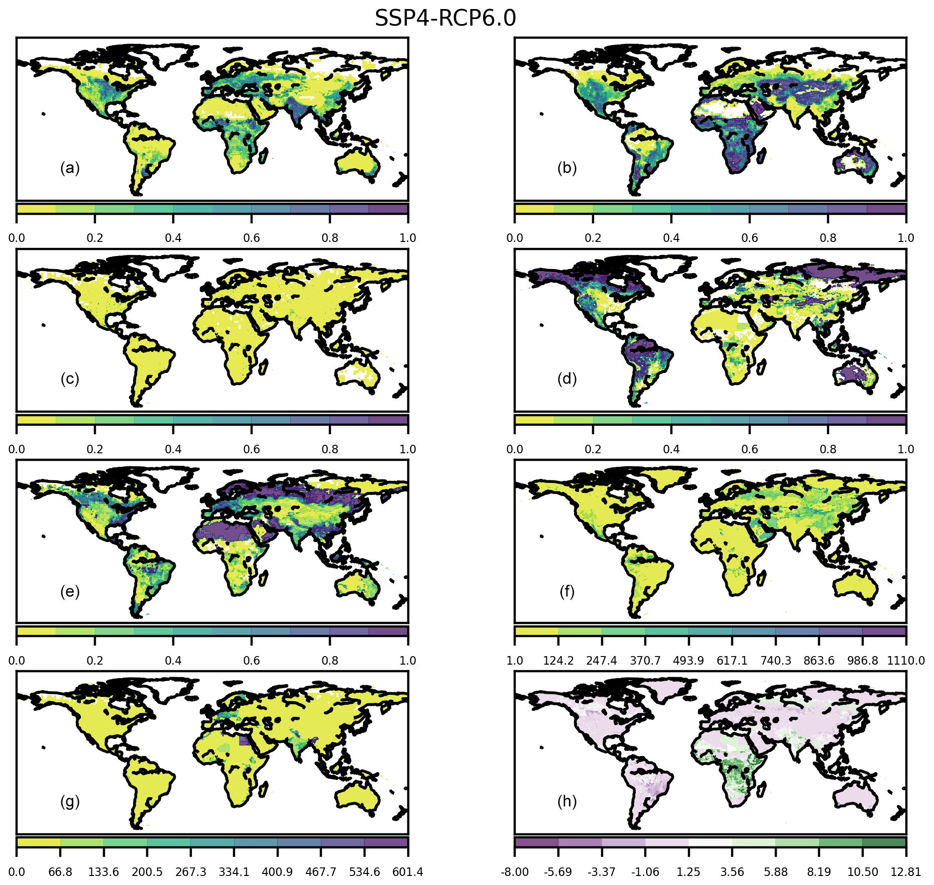
Figure A1 Maps for the year 2100 for the SSP4-RCP6.0 scenario showing the following: (a) the fraction of each grid cell occupied by cropland; (b) the fraction of each grid cell occupied by pasture; (c) the fraction of each grid cell occupied by urban land; (d) the fraction of each grid cell occupied by primary vegetation; (e) the fraction of each grid cell occupied by secondary vegetation; (f) the mean age (in years) of secondary lands in each half-degree grid cell; (g) the mean gross transitions (km² yr⁻¹) over a 20-year interval for each grid cell; and (h) the mean net transitions (km² yr⁻¹) over a 20-year interval for each grid cell.

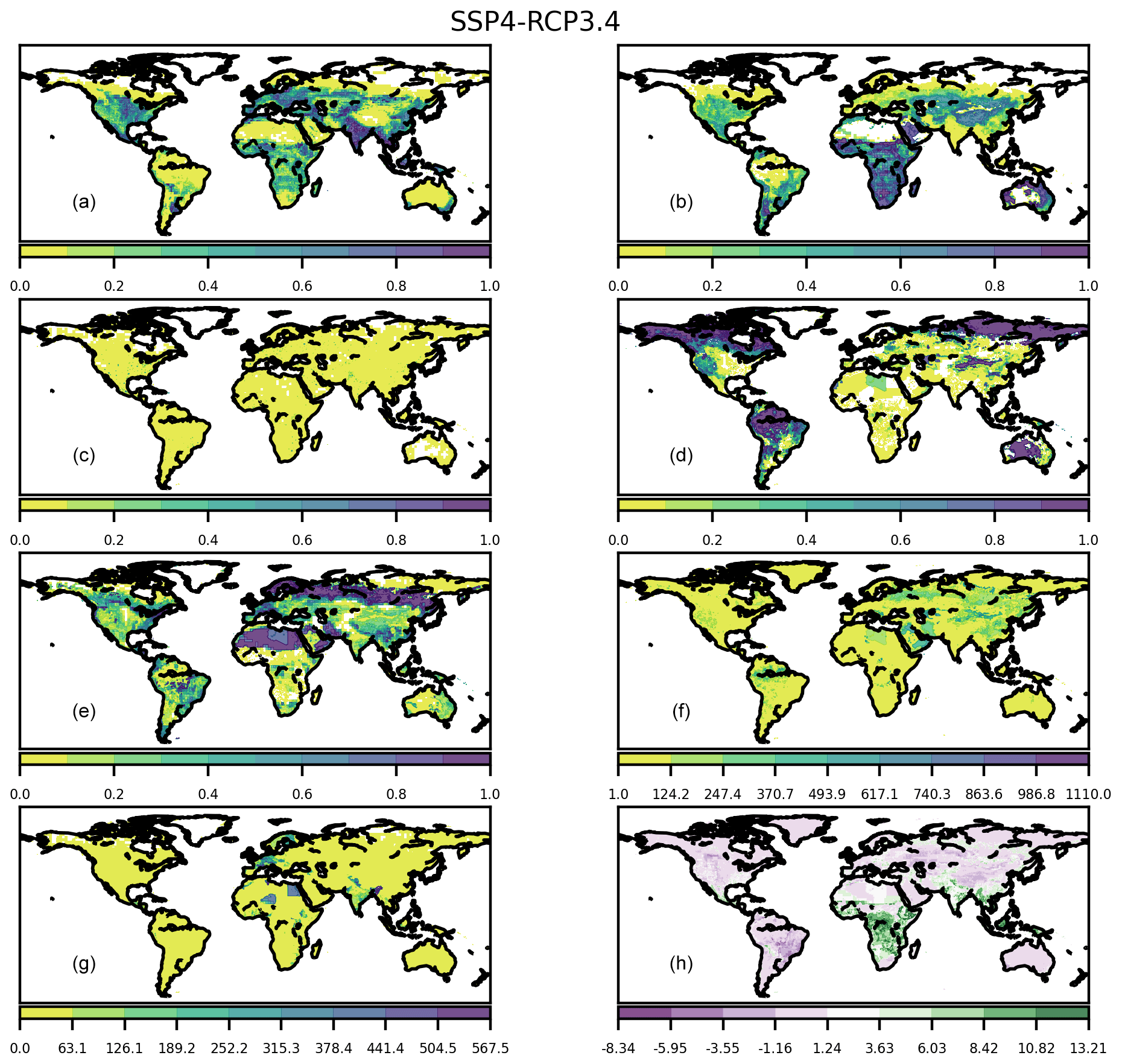
Figure A2 Maps for the year 2100 for the SSP4-RCP3.4 scenario showing the following: (a) the fraction of each grid cell occupied by cropland; (b) the fraction of each grid cell occupied by pasture; (c) the fraction of each grid cell occupied by urban land; (d) the fraction of each grid cell occupied by primary vegetation; (e) the fraction of each grid cell occupied by secondary vegetation; (f) the mean age (in years) of secondary lands in each half-degree grid cell; (g) the mean gross transitions (km² yr⁻¹) over a 20-year interval for each grid cell; and (h) the mean net transitions (km² yr⁻¹) over a 20-year interval for each grid cell.

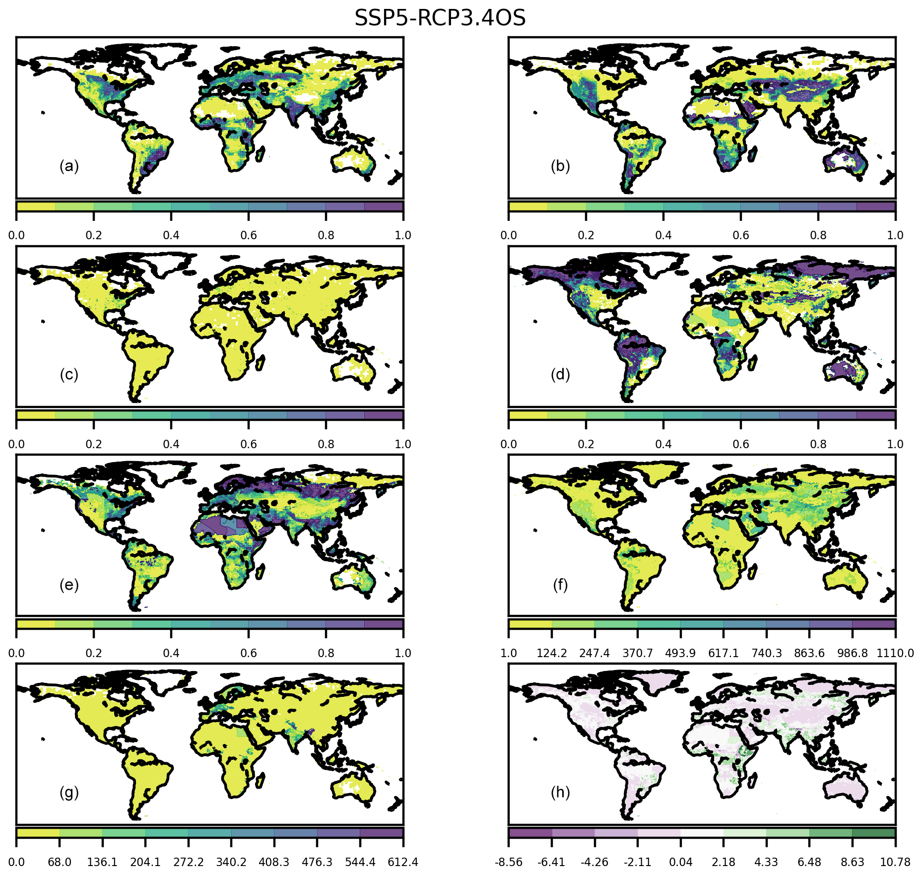
Figure A3 Maps for the year 2100 for the SSP5-RCP3.4OS scenario showing the following: (a) fraction of each grid cell occupied by cropland; (b) the fraction of each grid cell occupied by pasture; (c) the fraction of each grid cell occupied by urban land; (d) the fraction of each grid cell occupied by primary vegetation; (e) the fraction of each grid cell occupied by secondary vegetation; (f) the mean age (in years) of secondary lands in each half-degree grid cell; (g) the mean gross transitions (km² yr⁻¹) over a 20-year interval for each grid cell; and (h) the mean net transitions (km² yr⁻¹) over a 20-year interval for each grid cell.

Figure A4 Maps for the year 2100 for the SSP1-RCP1.9 scenario showing the following: (a) the fraction of each grid cell occupied by cropland; (b) the fraction of each grid cell occupied by pasture; (c) the fraction of each grid cell occupied by urban land; (d) the fraction of each grid cell occupied by primary vegetation; (e) the fraction of each grid cell occupied by secondary vegetation; (f) the mean age (in years) of secondary lands in each half-degree grid cell; (g) the mean gross transitions (km² yr⁻¹) over a 20-year interval for each grid cell; and (h) the mean net transitions (km² yr⁻¹) over a 20-year interval for each grid cell.