the Creative Commons Attribution 4.0 License.
the Creative Commons Attribution 4.0 License.
 | 19 Oct 2020
A multi-isotope model for simulating soil organic carbon cycling in eroding landscapes (WATEM_C v1.0)
Zhengang Wang
Kristof Van Oost
There is increasing recognition that lateral soil organic carbon (SOC) fluxes due to erosion have imposed an important impact on the global C cycling. Field and experimental studies have been conducted to investigate this topic. It is useful to have a modeling tool that takes into account various soil properties and has flexible resolution and scale options so that it can be widely used to study relevant processes and evaluate the effect of soil erosion on SOC cycling. This study presents a model that is capable of simulating SOC cycling in landscapes that are subjected to erosion. It considers all three C isotopes (12C, 13C and 14C) with flexible time steps and a detailed vertical solution of the soil profile. The model also represents radionuclide cycling in soils that can assist in constraining the lateral and vertical redistribution of soil particles within landscapes. The model gives a three-dimensional representation of soil properties including 137Cs activity, SOC stock, and δ13C and Δ14C values. Using the same C cycling processes in stable, eroding and depositional areas, our model is able to reproduce the observed spatial and vertical patterns of C contents, δ13C values, and Δ14C values. This indicates that at the field scale with a similar C decomposition rate, physical soil redistribution is the main cause of the spatial variability of these C metrics.
- Article
(4800 KB) - Full-text XML
- BibTeX
- EndNote


Soil organic carbon (SOC) is the largest organic C pool on land, with approximately 1550 Pg C in the upper meter of soil (Lal, 2008). This is about 2 times the C in the atmosphere (ca. 760 Pg C). The annual C flux between soil and the atmosphere is ca. 60 Pg C, which makes atmospheric CO2 sensitive to SOC cycling. SOC stock is a balance between input fluxes and output fluxes, which is controlled by various factors such as soil structure, soil parent material, soil pH, climate, and land use and management. Climate is an important controlling factor on SOC cycling as it is closely related to the rate of both C input and decomposition (e.g., Cox et al., 2000; Davidson and Janssens, 2006). The terrestrial net primary production and SOC decomposition rate generally decrease with increasing temperature (Koven et al., 2017). Globally, SOC stock decreases with increasing temperature (Jobbágy and Jackson, 2000). Land use is another important factor because different vegetation supplies SOC to the soil at different rates (Mahowald et al., 2017; Maia et al., 2010). The stable isotopic composition of SOC is affected by factors such as vegetation type (C3 vegetation versus C4 vegetation) and the Suess effect (Tans et al., 1979). Also, SOC can be enriched in 13C during the processes of SOC degradation due to preferential mineralization of 12C (Natelhoffer and Fry, 1988).
Recent studies have shown that lateral soil redistribution by erosion could also impose an important impact on SOC stock and soil–atmosphere C exchange (Chappell et al., 2016; Doetterl et al., 2016). During erosion events, soil aggregates are broken by raindrops and overland flow, which can enhance SOC decomposition (Van Hemelryck et al., 2011). In the eroding region, SOC in the topsoil is removed by erosion, resulting in depletion of SOC. SOC is added to soil minerals that are moved upwards from below due to soil erosion by inputs from plants (Harden et al., 1999). SOC deposited in depositional settings is buried to depth, and the buried SOC is well preserved (Van Oost et al., 2012). This lateral redistribution of SOC and the consequent disturbance of SOC cycling of both eroding and depositional regions result in spatial variability in SOC stocks and properties. It has been found that eroding sites are depleted of SOC compared to stable sites, while depositional sites are enriched in SOC compared to stable sites in agricultural fields (Li et al., 2007; Van Oost et al., 2005; Yoo et al., 2005). Soil redistribution could lead to differences in SOC stability between eroding and depositional areas. Berhe et al. (2008) found that SOC decomposes at faster rates in eroding areas compared to depositional areas using signatures of 14C. Wang et al. (2014) reported that SOC mineralization rates in eroding soil profiles are higher than those of depositional soil profiles from results of laboratory soil incubation. Radioactive C isotopes such as 14C give information on the SOC turnover time, and it is a useful tool to investigate long-term SOC cycling (Trumbore, 2009). SOC redistribution has been found to have an effect on SOC radioactive C isotope composition, with eroding areas more negative compared to depositional areas (Berhe et al., 2008).
Apart from the empirical studies mentioned above, various models have been developed to simulate soil erosion and SOC cycling. At the event scale, there are models simulating processes such as rainfall detachment, sediment entrainment and sediment transport (e.g., Hairsine and Rose, 1992a, b). Some models separate sediments into different grain sizes, and these models are suitable for simulating size selectivity in erosion and deposition (Nearing, 1989; Van Oost et al., 2004). These models are further modified to simulate the selectivity of SOC in erosion and deposition (Wilken et al., 2017). Models based on USLE (Universal Soil Loss Equation) utilize annual mean precipitation as model input to simulate long-term soil erosion (Renard et al., 1997). Given that atmospheric fallouts of 137Cs are closely adsorbed on soil particles, 137Cs inventories in soils are widely used to evaluate erosion rates (Gaspar et al., 2013; Quine et al., 1997). Soil erosion models have further added processes of 137Cs deposition, decay and redistribution associated with soil particles so that they can be calibrated using observed 137Cs data (Van Oost et al., 2003).
C turnover models have been developed under the condition of stable landscapes (i.e., free of erosion and deposition) to explore the effects of climate, land use and soil environment on SOC cycling. The decomposition of C is often represented by a first-order kinetic rate. Because SOC is a complex of different components, it is often represented by various pools with respect to C input and decomposition rates in models such as CENTURY (Parton et al., 1987), ICBM (Andren and Katterer, 1997) and RothC (Coleman and Jenkinson, 1995). C fractions obtained in laboratories have been related to C pools in models and have been used to calibrate model parameters to investigate the turnover of various C pools (Skjemstad et al., 2004; Wang et al., 2015a; Zimmermann et al., 2007).
These multiple-pool C models were further integrated with soil erosion models to make them applicable in eroding landscapes. For instance, a study adding erosion processes to the CENTURY model has been used to investigate the balance between the lateral SOC loss by erosion and in situ replacement of lost SOC by photosynthesis in eroding areas, and it has been found that proper management is important to maintain the dynamic replacement of lost C (Harden et al., 1999). At the depositional areas, Wang et al. (2015b) calibrated a profile-scale model integrating erosion and SOC cycling processes using observed SOC content and long-term depositional rate, and it was found that sedimentation rate plays an important role in determining burial efficiency of SOC in colluvial settings. Models have also been developed to investigate the relationships between erosion, crop productivity and SOC cycling (Bouchoms et al., 2019). At the field scale, models that combine SOC redistribution by erosion and SOC dynamics are now able to reproduce the spatial heterogeneity of SOC stock in fields under land uses with eroding areas depleted of SOC and depositional areas enriched in SOC (Liu et al., 2003; Rosenbloom et al., 2001, 2006; Van Oost et al., 2005; Yoo et al., 2005).
Carbon isotopes have also been included in SOC cycling models to constrain model parameters or explore controlling factors. Baisden et al. (2002) used C and N isotopes to simulate the turnover and transport of SOC along soil depth and showed that hydrological conditions had an important role in controlling the vertical transport of SOC. Also, an SOC cycling model integrating C isotope discrimination was utilized to explore the effects of SOC decomposition and physical mixing on the formation of the vertical increase in δ13C values with the soil depth (Acton et al., 2013). Ahrens et al. (2014) used 14C signatures to constrain model parameters of a multi-pool SOC model using the Bayesian method, and the model was further applied to quantify the contribution of sorption, dissolved organic carbon transport and microbial interactions in determining the Δ14C values of soil profiles (Ahrens et al., 2015). Although field studies have identified the effects of soil redistribution on the profile of SOC isotopes (Berhe et al., 2008), relevant models are not developed yet. SOC models including C isotopes applicable in eroding landscapes would be helpful to fully understand the C isotope profiles as well as the spatial variability of SOC isotopic composition at the landscape scale.
Here, we integrate SOC and soil erosion models and present a model tool that is capable of simulating SOC dynamics in an eroding landscape. The objectives of this modeling tool are the following: (i) it should be a multiple C pool model that is able to represent the complexity of SOC and to be related to the measurable SOC fractions; (ii) it should include various C isotopes so that it could not only represent these C metrics but also use them to constrain the model; and (iii) it should be flexible in terms of spatial and temporal scales so that it would be applicable in various cases regarding spatial and temporal settings.
2.1 Study sites and field data
The first study site is located in the Belgian loam belt. The study area has a temperate climate with average annual precipitation of 750–800 mm and a mean annual temperature of approximately 9.5 ∘C. Soils in the study area are mainly loess-derived Luvisols with a high silt content (>70 %) and relatively low clay (<15 %) and sand (<20 %) contents (Beuselinck et al., 2000). Arable lands with wheat, maize, sugar beet and potato are the main land use type of the study area. Soil samples were collected from cropland fields with rolling topography, from which soil cores were taken on plateau (with no erosion), convex slope (with erosion) and concave slope (with deposition) areas. SOC contents were measured with a vario MAX CN Macro elemental analyzer (Elementar Analysensysteme GmbH, Germany), while δ13C was measured with an ANCA 20-20 GSL mass spectrometer (Sercon Ltd, UK). The inorganic C was removed from soil samples using the HCl fumigation method proposed by Harris et al. (2001).
This study also used published SOC and Δ14C data in Berhe et al. (2008) to evaluate the developed model. The data were collected at Tennessee Valley in Marin County, northern California (37.9∘ N latitude, 122.6∘ W longitude). The climate at Tennessee Valley is Mediterranean, with a mean annual precipitation of 1050 mm and a mean annual temperature of 14 ∘C. The dominant vegetation cover in the study area is represented by Mediterranean grasses and a coastal shrub (Baccharis pilularis, coyote brush). Soils at Tennessee Valley are derived from chert, greenstone and greywacke sandstone bedrock of the Franciscan assemblage. Soil profiles at the position of plateau (no erosion), convex slope (erosion), concave slope (deposition) and valley (deposition) areas were sampled along a slope. C content was measured with a Carlo Erba elemental analyzer, while the radiocarbon content was measured using accelerator mass spectrometry (AMS) following the methods of Trumbore et al. (1989).
2.2 WATEM_C
Here we present WATEM_C that simulates the redistribution of eroded soil and associated C within the catchment and its effects on the dynamics of SOC. The soil redistribution by water erosion is based on WATEM (Water And Tillage Erosion Model; Van Oost et al., 2000), while the simulation of C dynamics is based on a three-pool C model (Wang et al., 2015a). All three C isotopes (12C, 13C and 14C) are included in our model. Soil advection and diffusion through the soil profile are also included in the model. The model uses a flexible time step and vertical resolution of the soil profile so that it can be applied in various settings.
2.2.1 Water erosion
The RUSLE (Revised Universal Soil Loss Equation) (Renard et al., 1997) is used to simulate the long-term potential water erosion (Epot; kg m−2 yr−1):
where R is the rainfall erosivity (MJ mm ha−1 h−1 yr−1), K is soil erodibility (kg h MJ−1 mm−1), L and S are slope length and steep factors, and C and P are factors for cover management and support practices.
The local erosion rate is considered to be equal to the potential erosion rate if the potential erosion rate does not exceed the local transport capacity. The local transport capacity (Tc; kg m−1 yr−1) is calculated as
where ktc is the transport capacity coefficient (m). In a grid cell, if its sediment inflow exceeds its local transport capacity, the amount of material transported through the grid equals the local transport capacity, while the remainder is deposited in the grid.
A routing algorithm was applied to transfer the mobilized sediments towards the catchment outlet. First, the grids of the study area were sorted in descending order based on the digital elevation model (DEM). Then, after comparing the local transport capacity of a grid cell with the incoming sediment and the locally produced sediment (Van Oost et al., 2000), sediments were routed downslope. Prediction of the flow direction was based on Takken et al. (2001).
The mobilization of SOC or 137Cs by erosion (Cero, kg m−2 yr−1) is estimated as
where Ctop is the content of a carbon isotope or 137Cs in the topsoil layer (%), Rero is the local erosion rate (kg m−2 yr−1) and ERero is the C enrichment ratio in the eroded sediments that equals the ratio of C content in the eroded sediments to that in the source soils.
The deposited SOC or 137Cs (Cdepo, kg m−2 yr−1) can be calculated as
where Csed is the content of a C isotope or 137Cs in the transported sediments (%), Rdepo is the local deposition rate (kg m−2 yr−1) and ERdepo is the C enrichment ratio in the deposited sediments that equals the ratio of the C content in the deposited sediments to that in the bulk transported sediments reaching the depositional sites.
The enrichment ratios of SOC or 137Cs in the mobilized sediments at the erosion sites or in the deposited sediments at the deposited sites are found to be closely related to the local erosion or deposition rates (Schiettecatte et al., 2008; Wang et al., 2010). Thus, the enrichment ratios of SOC or 137Cs in the mobilized and deposited sediments are calculated as
where a, b and d are coefficients.
2.2.2 Soil C turnover
In our model, the three C isotopes (12C, 13C and 14C) are distinguished. As called in the CENTURY model (Parton et al., 1987), each C isotope is divided into three pools that are referred to as active, slow and passive pools. The decomposition of these C pools is described using the following differential equations.
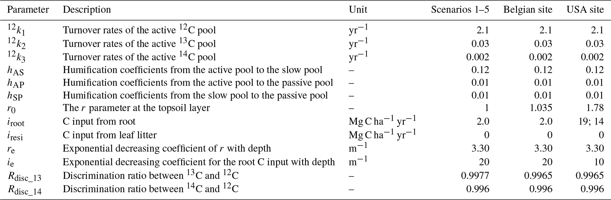
Here, nA(z,t), nS(z,t) and nP(z,t) (%) are the contents of the active, slow and passive pools of C isotope n at depth z (m) and time t (year), respectively; ni(z) (Mg C yr−1) is the input of C isotope n at depth z (m); hAS is the humification coefficient from the active pool to the slow pool, hAP from the active pool to the passive pool, and hSP from the slow pool to the passive pool, respectively; r(z) is a coefficient modifying the variation of the C mineralization rate, which denotes the effect of local environmental factors (temperature, humidity, aeration, etc.) at depth z (m); and nk1, nk2 and nk3 (yr−1) are the turnover rates at the reference condition (i.e., r(z)=1) of the active, slow and passive pools of C isotope n, respectively.
12C is preferentially lost through microbial respiration compared to 13C and 14C due to its lower atomic weight (Natelhoffer and Fry, 1988). We used a discrimination ratio to denote the difference in mineralization between isotopes, and thus the decomposition rate of a 13C pool (13km, yr−1) can be calculated as
where Rdisc_13 is the discrimination ratio between 13C and 12C, and 12km is the decomposition rate of the corresponding 12C pool.
Similarly, the decomposition rate of a 14C pool (14km, yr−1) can be calculated as
where Rdisc_14 is the discrimination ratio between 14C and 12C.
The r parameter represents the effect of environmental factors affecting C respiration at a given depth, and it is calculated as
where r0 is the value of the r parameter at the topsoil layer, and re (m−1) is an exponential decreasing coefficient.
The input of the C isotopes from plant roots decreases exponentially with depth (Gerwitz and Page, 1974; Van Oost et al., 2005):
where ni0 is the input of C isotope n at the topsoil layer (Mg C yr−1), ni(z) (Mg C yr−1) is the input of C isotope n at depth z (m) and ie (m−1) is an exponential decreasing coefficient.
The δ13C values are expressed in terms of per mill (‰) deviation:
where (13C∕12C)Sample is the abundance ratio of 13C to 12C of the soil sample, and (13C∕12C)PDB is the ratio of the Pee Dee Belemnite (PDB) as the original standard.
Thus, the 13C input can be calculated as
where 13i is the 13C input (Mg C ha−1 yr−1) from plants, 12i is the 12C input from plants and δ13C(t) is the δ13C value of C input at time t (year).
We use the atmospheric Δ14C record as a proxy for the isotopic ratio of C input via root and leaf litter input (Hua and Barbetti, 2004). In this paper, the following definition of Δ14C (‰) is used (Stuiver and Polach, 1977):
where (14C∕12C)Sample denotes the 14C :12C ratio of the sample, and AABS denotes the 14C :12C ratio of the standard. AABS is set to be (Karlen et al., 1965; Stuiver, 1980).
The 14C input can then be calculated as
where 14i is 14C input (Mg C ha−1 yr−1) from plants, and is the atmospheric Δ14C signal at time t (year).
2.2.3 Soil profile evolution due to erosion
In the model, soil profiles are represented as a series of soil layers with equal depths. Given that C input and SOC decomposition rate are related to soil depth, SOC cycling is simulated in each layer independently. Because erosion and deposition change the depth of soil profiles, the model updates the depth of soil profiles and the carbon content of each soil layer every time step. At the eroding locations, soils are removed from the top layer and the soil profile is truncated by the amount of eroded soil. In the meantime, SOC is also lost with the local C enrichment ratio. To keep the soil layer with fixed thickness, soils and associated SOC from soil layers below are incorporated into the upper soil layer at the erosion rate. At the depositional locations, because the top layer is buried by the deposited sediments at the deposition rate, soils and associated SOC are moved downward. For all the soil profiles, the component pools of each C isotope of every layer are updated by homogeneously mixing the component materials every time step.
2.2.4 Advection and diffusion
The vertical transport of mineral and organic components of soil is a complex phenomenon driven by a number of distinct mechanisms such as bioturbation (Jagercikova et al., 2017; Johnson et al., 2014) and chemical mobilization (Taylor et al., 2012). We use the advection–diffusion equation to model vertical transport:
where F(z,t) is the concentration of a soil constituent (such as a C isotope pool or 137Cs) at depth z (m) at time t (year), v(z) (m yr−1) is the advection term at depth z (m) and K(z) (m yr−1) is a diffusion-type mixing coefficient at depth z (m).
K and v are both depth-dependent and are represented using a sigmoidal scaling function:
where vd (m−1) is the depth attenuation of advection, ct (m) is a constant that is set to 0.15 m and v0 (m yr−1) is the value of v at the topsoil layer.
Kd (m−1) is the depth attenuation of diffusion, and K0 (m yr−1) is the value of K at the topsoil layer.
2.2.5 137Cs dynamics
137Cs is an artificial nuclear radioactive isotope from nuclear tests and reactor incidents. The 137Cs in the soil mainly originates from bomb experiments between 1950 and 1970. It falls from the atmosphere primarily in association with precipitation and is rapidly adsorbed to soils by clay materials. As the fallout is well constrained, 137Cs has been widely used for tracing the movement of soil and sediment particles in erosion studies (Ritchie and McHenry, 1990). WATEM_C reads the values of the local 137Cs fallout. The model then simulates the redistribution of 137Cs by soil erosion and deposition at the land surface associated with soil particles (Eqs. 1–6). The model also simulates the downward movement of 137Cs in the soil profile by advection and diffusion (Eq. 18). The decay of 137Cs (half-life of 30.23 year) is also represented in the model:
where Cs(z,T) (%) is 137Cs content at soil depth z (m) at time t (year), Rp (equal to 0.977) is the fraction of 137Cs preserved after decay of 1 year and T (year) is the time step of the model iteration.
2.2.6 Model implementation
In order to make the model applicable at various temporal and spatial resolutions, the time step of model iteration and the vertical resolution of the soil profile were not fixed but modifiable as parts of the model input parameters. Given the long-term temporal iteration in SOC cycling processes and the possible large spatial regions where the model may apply, the model was developed using a computation-efficient language (Pascal). The compiled executable file can then be called in other environments such as R (R Development Core Team, 2011), for which the preparation of the input maps is easier. In our model, the default values of the input parameters were given, and at the same time users are allowed to assign custom values to the input parameters in the R environment when calling the executable file. The description and relevant parameters regarding SOC cycling used in this study are listed in Table 1. For the initialization of the 137Cs profile, the model first checked if the beginning year of the model simulation was earlier than the beginning of 137Cs fallout. If earlier, the initial 137Cs profile was set to be zero; if not earlier, the model was run from the beginning of 137Cs fallout to the beginning year of the model simulation with relevant parameter values of soil advection and diffusion to generate the initial 137Cs profile. For the initialization of C profiles, the initial profile of each C pool was set to be the equilibrium C profile under specific conditions to ensure that the initial C profile was realistic for the study site, i.e., the C profile that made the C input equal to the C mineralization, which was determined by model parameters such as C inputs, C turnover rates and humification coefficients. The model had input parameters of the initial δ13C and Δ14C values of the top and bottom soil layers, and the profiles of δ13C and Δ14C values were then generated by a liner interpolation based on the values of the top and bottom soil layers. The model was then run for a parameter-defined period to get the profiles to reach equilibrium.
2.2.7 Model application
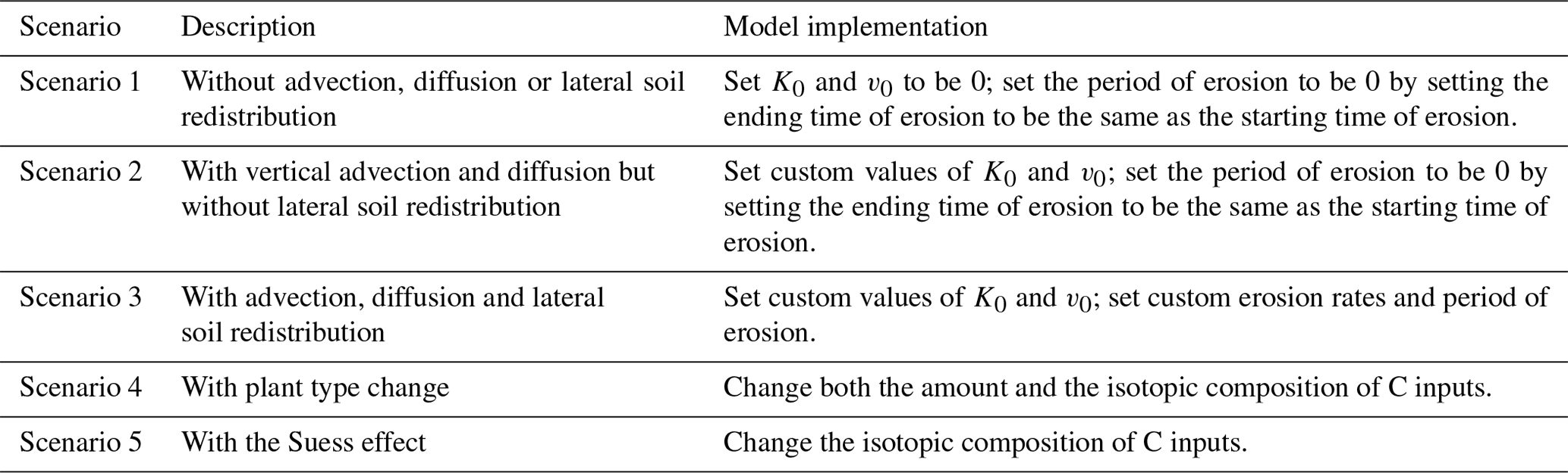
Five model scenarios was tested in this study (Table 2). A set of three scenarios was assumed in order to investigate the effect of advection and diffusion as well as lateral soil redistribution by erosion on the spatial and vertical distribution of SOC and δ13C and Δ14C values at the landscape scale. Scenario 1 is a scenario without advection, diffusion or lateral soil redistribution. Scenario 2 is a scenario with vertical advection and diffusion but without lateral soil redistribution. Scenario 3 is a scenario with advection, diffusion and lateral soil redistribution. In order to investigate the effect of plant type change and the Suess effect on the δ13C values of soil profiles, the model was applied in another set of three scenarios. Given that advection and diffusion are common in soils, we used the scenario with only advection and diffusion as the reference scenario, i.e., Scenario 2 defined above. The other two scenarios are Scenario 4 with plant type change and Scenario 5 with the Suess effect.
The model was also evaluated using observed C, δ13C and Δ14C soil profiles. Given that an important objective of this study is to investigate the effects of vertical soil advection and diffusion as well as lateral soil redistribution on the profiles of C, δ13C and Δ14C, the model was optimized for parameters of K0, v0 and the soil redistribution rate, while the other model parameters were set to be realistic values. For the study site in Belgium, the soil redistribution rates varied between soil profiles due to their locations on the hillslope, while the other parameters were set to be the same among soil profiles. For the study site in the USA, the soil redistribution rates varied between soil profiles. As noted by Berhe et al. (2008), the grass types vary between slope positions. Also, the top C contents showed great differences between profiles (Fig. 1a). Therefore, the C inputs were set to be different between soil profiles. The other parameters were set to be the same among soil profiles for the study site in the USA. The period of erosion was set to be 100 years. The model calibration was performed by comparing the agreement of the simulations and observations, which included both C contents and C isotopic composition (δ13C values were available at the Belgian study site, while Δ14C data were available at the USA study site). A weight factor was introduced to make sure that both the C content and C isotopic composition played equivalent roles in the model calibration.
MRMSE is the modified root mean square error of the model, SCj (%) is the simulated C content of sample j, OCj (%) is the observed C content of sample j, Cj is the number of C content observation, SDC (%) is the standard deviation of the observed C contents of all the samples, SIj (‰) is the simulated isotopic composition of sample j, OIj (‰) is the observed C isotopic composition of sample j, Ij is the number of the observed C isotopic composition of all the samples and SDI (‰) is the standard deviation of the observed C isotopic composition of all the samples.
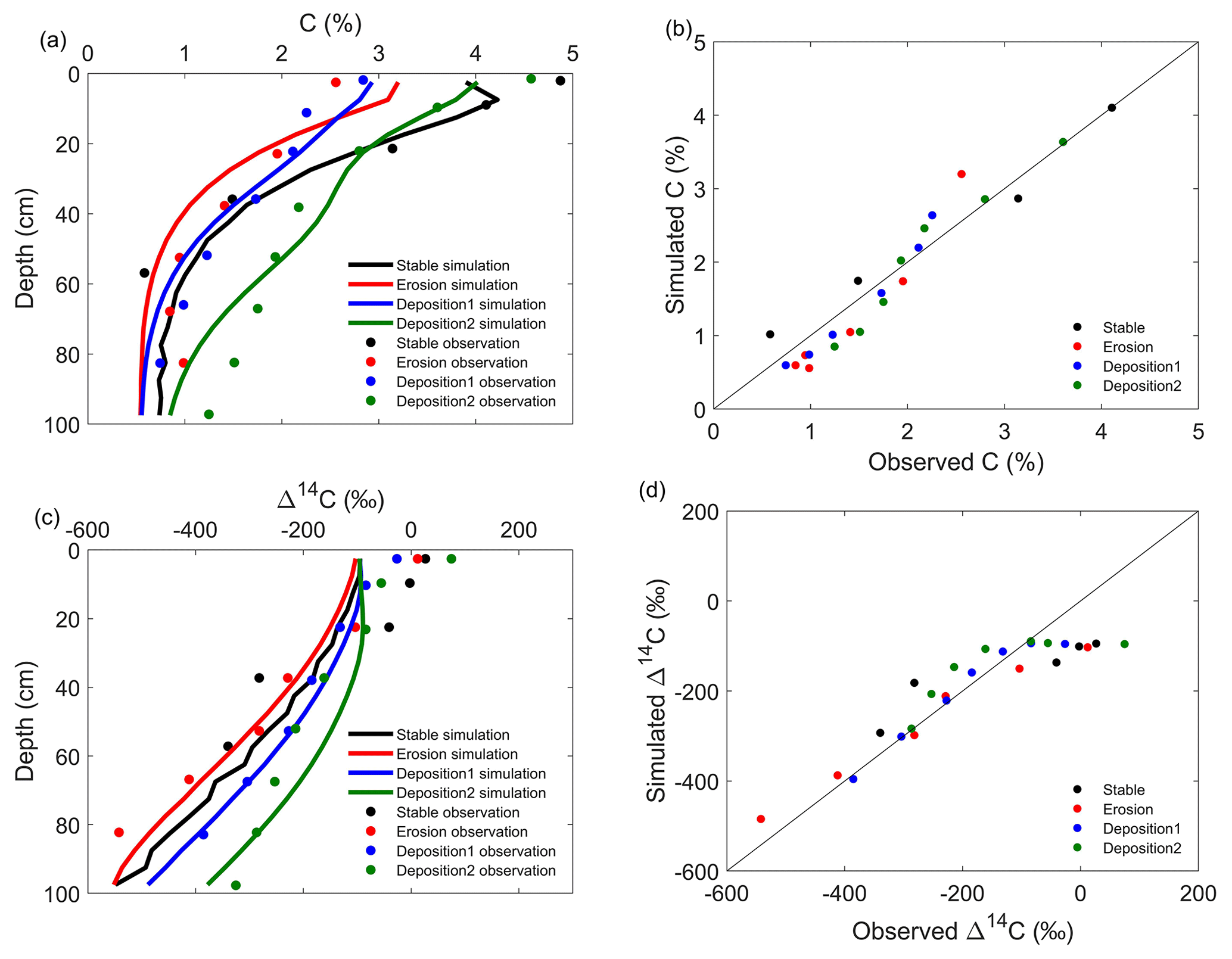
Figure 1Observed and simulated C content and Δ14C values of stable, erosion and depositional areas at the USA study site. Observed and simulated C contents in the format of profiles (a) and 1 : 1 lines (b); observed and simulated Δ14C values in the format of profiles (c) and 1 : 1 lines (d).
In order to quantify the effects of C decomposition, vertical soil advection and diffusion, and lateral soil redistribution on the C, δ13C and Δ14C profiles, comparisons were performed between the reference profiles (i.e., profiles under the condition of Scenario 1) and profiles under a given condition of SOC decomposition, vertical soil advection and diffusion, and lateral soil redistribution using root mean square error (RMSE):
where SVi is the simulated value of C content or C isotopic composition of soil layer i, OVi is the observed value of C content or C isotopic composition of soil layer i, and n is the number of soil layers.
The Fourier amplitude sensitivity test (FAST) (Cukier et al., 1973, 1975) was applied using simulations obtained in a Monte Carlo approach to assess the contribution associated with relevant parameters. The FAST method is based on the analysis of variance (ANOVA) decomposition, which quantifies the relative contribution of only one given parameter to the total variance of the model output. Eight parameters of the model relevant to C decomposition (r0 and re), soil advection and diffusion (K0, Kd, v0 and vd), and soil redistribution (soil redistribution rate and erosion time) were tested in 10 000 Monte Carlo scenarios. The values of these parameters were derived from a random distribution within a realistic range (r0: 0.5–1.5; re: 2.6–4 m−1; K0: 0.005–0.1 m yr−1; Kd: 0.005–0.015 m−1; v0: 0.01–0.02 m yr−1; vd: 0.005–0.015; soil redistribution rate: −1 to 1 mm yr−1; erosion time: 1–100 years) for each Monte Carlo scenario. No correlations among these input parameters were assumed for sample generation. The FAST was performed using the MATLAB package developed by Cannavo (2012).
3.1 Model calibration
The optimal parameter values obtained after model calibration are reported in Tables 3 and 4. The model simultaneously simulated both the observed C content and C isotopic composition profiles well, with the MRMSE being 2.26 and 4.46 for the Belgian and the USA study sites, respectively (Figs. 1 and 2). The model not only reproduced the horizontal difference of the C, δ13C and Δ14C profiles between soil profiles well, but the vertical patterns of these profiles were also well represented by the model, except the model underestimated the Δ14C values at the topsoil layers (Fig. 1c).
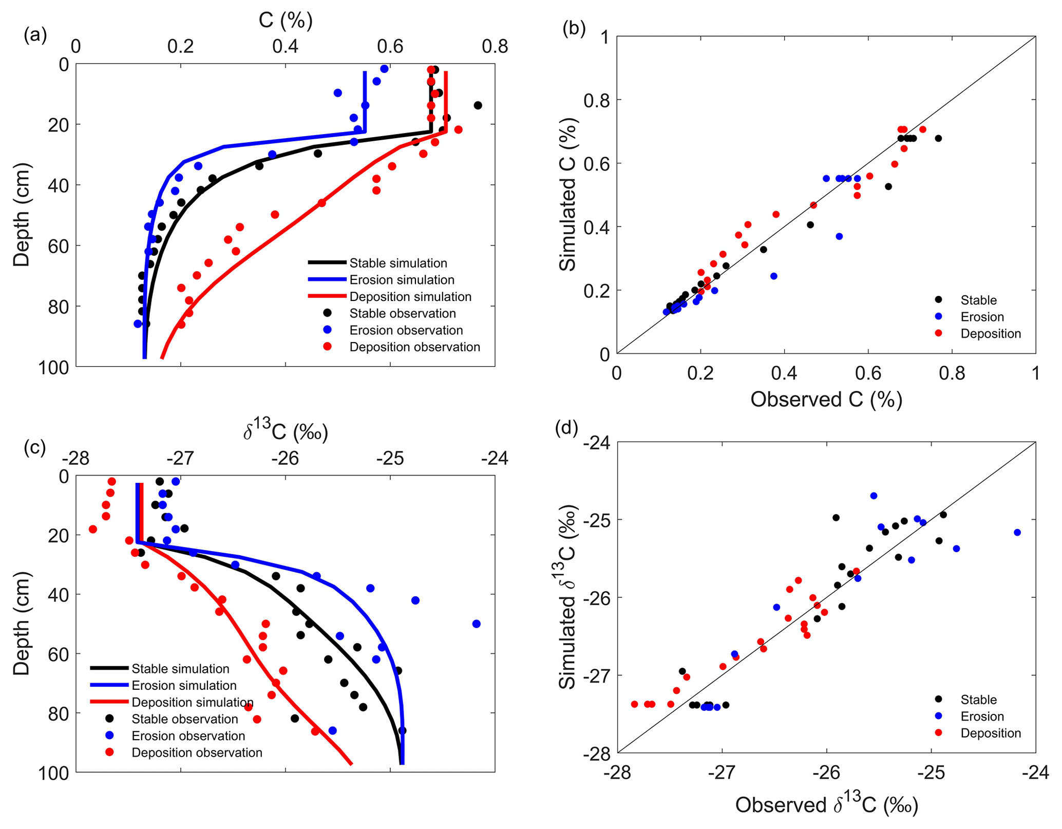
Figure 2Observed and simulated C content and δ13C values of stable, erosion and depositional areas at the Belgian study site. Observed and simulated C contents in the format of profiles (a) and 1 : 1 lines (b); observed and simulated δ13C values in the format of profiles (c) and 1 : 1 lines (d).
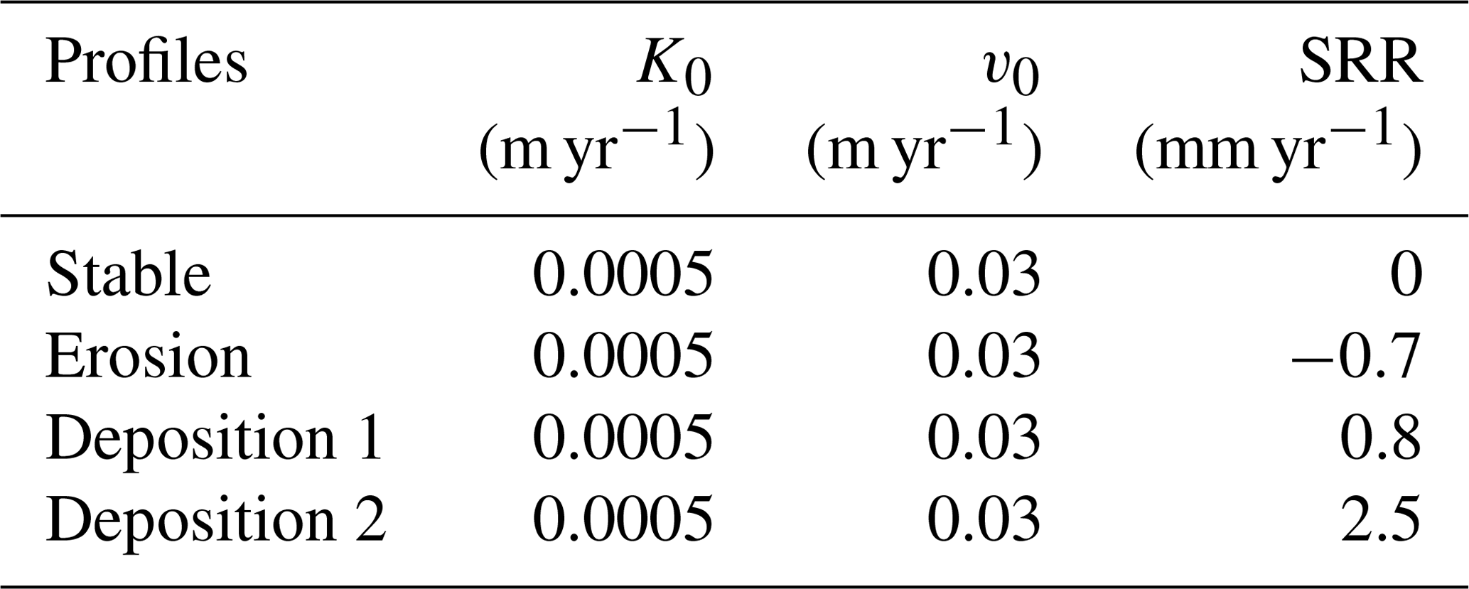
Table 3Calibrated optimal parameter values for the Belgian study site. Kd and vd were set to be 0.01 m−1 in the model calibration. The parameter values for SOC cycling are listed in Table 1. SRR indicates the soil redistribution rate.

Table 4Calibrated optimal parameter values for the USA study site. Kd and vd were set to be 0.01 m−1 in the model calibration. The parameter values for SOC cycling are listed in Table 1. SRR indicates the soil redistribution rate.
3.2 SOC
Our model is able to reproduce the general pattern of the SOC profile for decreasing SOC content with depth in all scenarios despite rates of advection, diffusion, erosion or deposition (Fig. 3). In Scenario 2, higher rates of soil advection and diffusion result in more SOC transferred to depth, and therefore the difference in SOC content between top layers and bottom layers is smaller under the condition of higher soil advection and diffusion rates compared to SOC profiles with lower advection and diffusion rates (Fig. 3b). In Scenario 3, eroding soil profiles contain less SOC compared to the stable soil profiles free of erosion and deposition, while soil profiles at the depositional area are enriched in SOC compared to the stable soil profile (Fig. 3c).
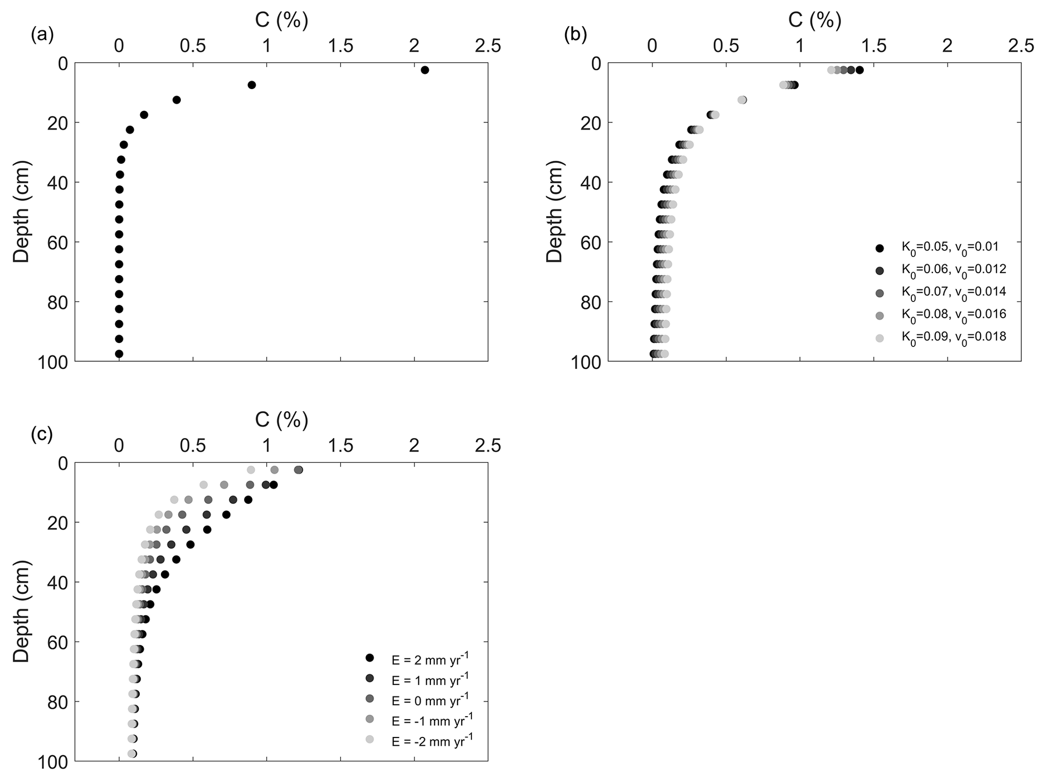
Figure 3The simulated C content profiles in (a) Scenario 1, (b) Scenario 2 and (c) Scenario 3. See Sect. 2.2.7 and Table 2 for descriptions of the scenarios. In (b), K0 (m yr−1) is the diffusion coefficient at the topsoil layer and v0 (m yr−1) is the advection term at the topsoil layer (Eq. 18). In (c), E indicates the soil redistribution rates, with negative values indicating erosion and positive values indicating deposition. K0 and v0 were set to be 0.09 m yr−1 and 0.018 m yr−1, respectively. In (b) and (c), both Kd and vd (depth attenuation of diffusion and advection) were set to be 0.01 m−1.
3.3 δ13C values
In Scenario 1, the δ13C profile shows no variation with depth (Fig. 4a). In Scenario 2, the δ13C profile decreases with depth (Fig. 4b). The δ13C values of the soil profile with higher soil advection and diffusion rates are more negative than that with lower soil advection and diffusion rates (Fig. 4b). In Scenario 3, the δ13C values of the eroding profile are less negative than those of the stable soil profile, while soil profiles at the depositional area have more negative δ13C values compared to the stable soil profile (Fig. 4c). Our simulation shows that δ13C values increase significantly when the vegetation is converted from C3 vegetation to C4 vegetation (Fig. 5). When the Suess effect is considered, the δ13C values are lower than in scenarios that do not consider the Suess effect (Fig. 5).
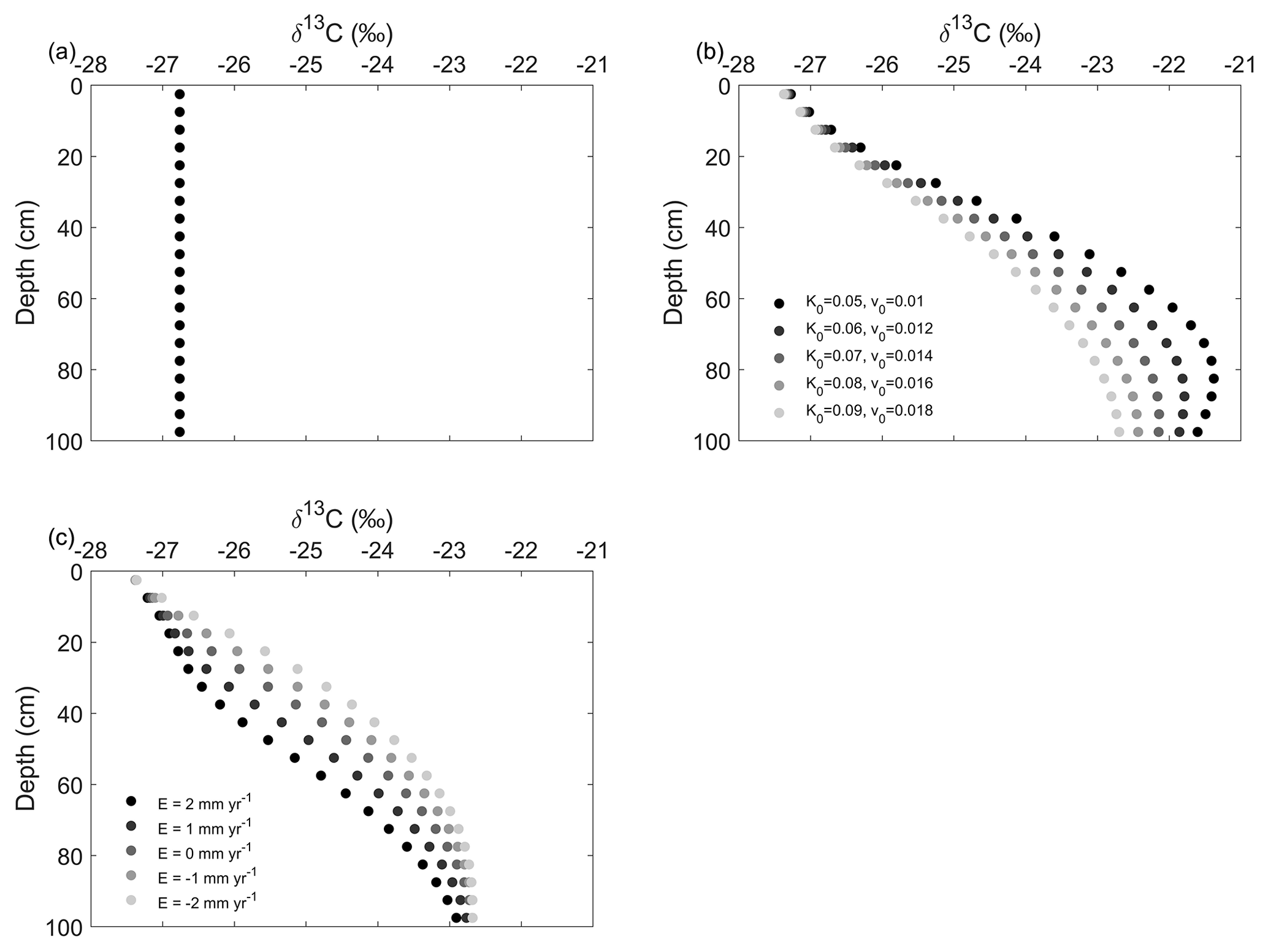
Figure 4The simulated δ13C profiles in (a) Scenario 1, (b) Scenario 2 and (c) Scenario 3. See Sect. 2.2.7 and Table 2 for descriptions of the scenarios. In (b), K0 (m yr−1) is the diffusion coefficient at the topsoil layer and v0 (m yr−1) is the advection term at the topsoil layer (Eq. 18). In (c), E indicates the soil redistribution rates, with negative values indicating erosion and positive values indicating deposition. K0 and v0 were set to be 0.09 and 0.018 m yr−1, respectively. In (b) and (c), both Kd and vd (depth attenuation of diffusion and advection) were set to be 0.01 m−1.

Figure 5Effects of plant type change and the Suess effect on the δ13C profiles. In the reference C3 plant scenario, the δ13C value of C inputs was set to be −26 ‰; in the Suess effect scenario, the δ13C value of C inputs decreased from −26 ‰ to −28.5 ‰ gradually. In the scenario of conversion from C3 plants to C4 plants, the δ13C value of C inputs was set to be −13 ‰ after vegetation change.
3.4 Δ14C values
Our model is able to reproduce the general pattern of decreasing Δ14C values with depth in all scenarios despite rates of soil advection, diffusion, erosion or deposition (Fig. 6). In Scenario 2, soil profiles with higher rates of advection and diffusion have higher Δ14C values compared to profiles with lower vertical transfer rates (Fig. 6b). In Scenario 3, eroding soil profiles have lower Δ14C values compared to the stable soil profiles, while soil profiles at the depositional area are enriched in 14C compared to the stable soil profile (Fig. 6c).

Figure 6The simulated Δ14C profiles in (a) Scenario 1, (b) Scenario 2 and (c) Scenario 3. See Sect. 2.2.7 and Table 2 for descriptions of the scenarios. In (b), K0 (m yr−1) is the diffusion coefficient at the topsoil layer and v0 (m yr−1) is the advection term at the topsoil layer (Eq. 18). In (c), E indicates the soil redistribution rates, with negative values indicating erosion and positive values indicating deposition. K0 and v0 were set to be 0.09 and 0.018 m yr−1, respectively. In (b) and (c), both Kd and vd (depth attenuation of diffusion and advection) were set to be 0.01 m−1.
3.5 Factors controlling C, δ13C and Δ14C profiles
C decomposition played the primary role in controlling the C, δ13C and Δ14C profiles, with the parameter r0 accounting for the major variance of the difference between reference profiles and Monte Carlo scenario profiles (Fig. 7). Soil advection and diffusion played a secondary role in controlling the C, δ13C and Δ14C profiles relative to C decomposition, with parameters K0 and r0 contributing more to the variance of the difference between reference profiles and Monte Carlo scenario profiles than parameters Kd and vd. Similarly, soil redistribution played a relatively secondary role compared to C decomposition, with the soil redistribution rate contributing more to the variance of the difference between reference profiles and Monte Carlo scenario profiles than the erosion time. For the C profile, the difference between reference profiles and Monte Carlo scenario profiles was mainly caused by parameter r0, while for the δ13C profile, both r0 and re played important roles. However, for the Δ14C profiles, r0, K0, v0 and the soil redistribution rate all accounted for more than 15 % of the variance of the difference between reference profiles and Monte Carlo scenario profiles.
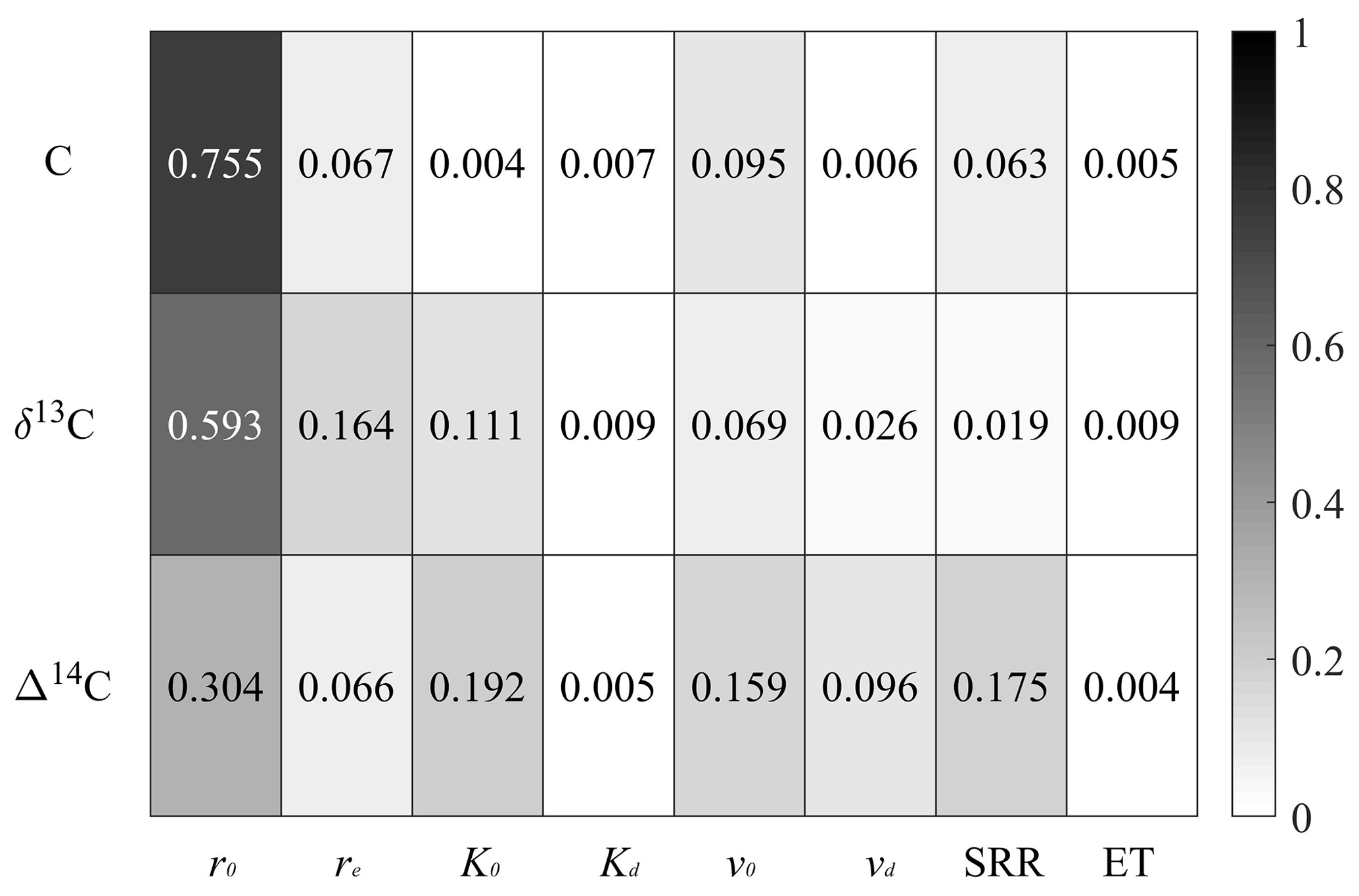
Figure 7The matrix of the proportion of variance of the difference between reference profiles and Monte Carlo scenario profiles caused by model parameters as indicated by the FAST coefficients. SRR indicates the soil redistribution rate, and ET indicates erosion time.
3.6 Spatial variability of soil properties
The model is able to generate a reasonable pattern of soil redistribution, with erosion occurring in upland areas and deposition occurring in footslope areas or valleys (Fig. 8b). Soil redistribution results in higher 137Cs inventories in depositional areas than eroding areas (Fig. 8c). The model is also able to generate the spatial variability of SOC stock and properties induced by erosion. The depositional area is enriched in SOC compared with the eroding area (Fig. 8d and e). SOC in the depositional area has lower δ13C values (Fig. 8f and g) and higher Δ14C values (Fig. 8h and i) compared to the eroding area.
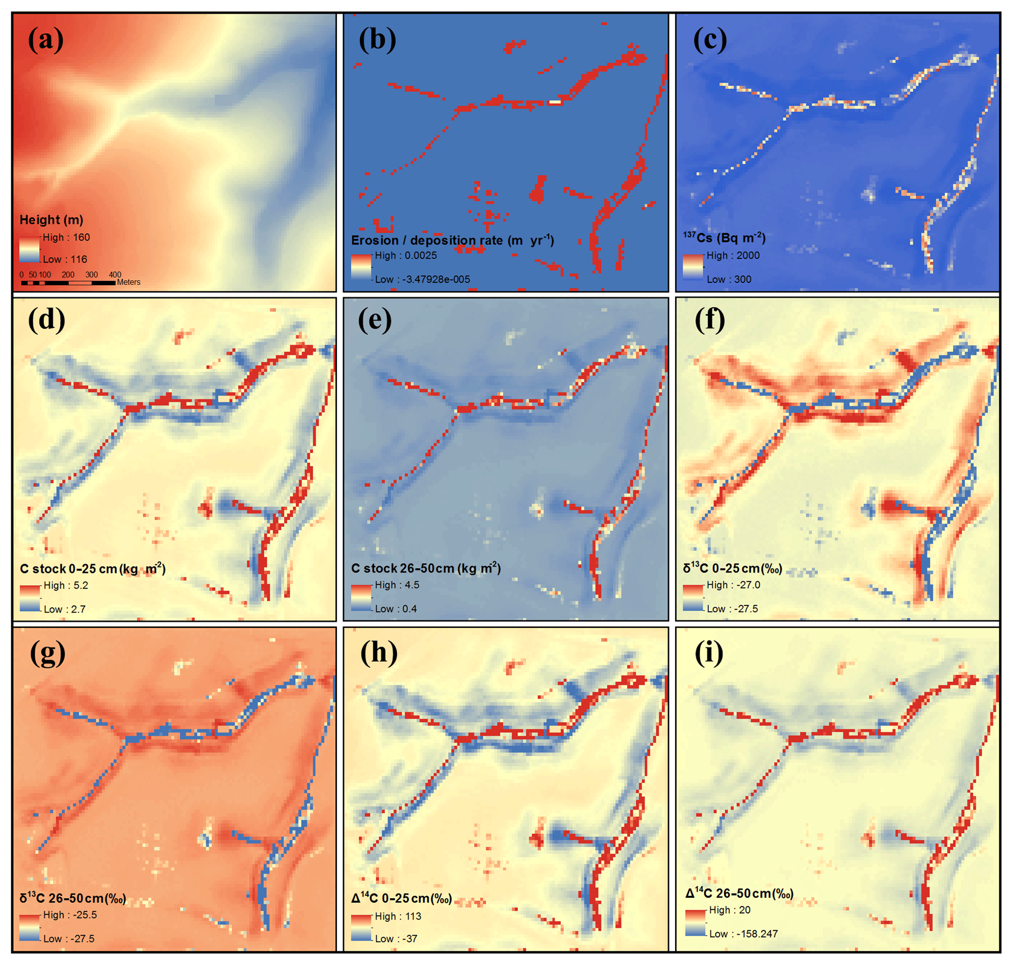
Figure 8Model simulations of erosion and erosion-induced spatial variability of SOC stock and isotopic compositions. (a) DEM (digital elevation model) of the field, (b) erosion and deposition rates (positive values indicate deposition and negative values indicate erosion), (c) 137Cs inventory, (d) C stock of topsoil (0–25 cm), (e) C stock of subsoil (26–50 cm), (f) δ13C values of topsoil (0–25 cm), (g) δ13C values of subsoil (26–50 cm), (h) Δ14C values of topsoil (0–25 cm), and (i) Δ14C values of subsoil (26–50 cm).
In Scenario 1, the shape of the SOC profile is determined by the vertical patterns of SOC input and decomposition rates, both of which decrease with depth. The fact that the basic shape of the SOC profile can be well represented in Scenario 1 shows that the pattern of C input and decomposition rates is the primary controlling factor on the SOC profile, while other factors such as advection, diffusion, erosion or deposition are relatively secondary (Fig. 3a). It is natural that higher rates of advection and diffusion would result in more SOC transferred to deep layers (Fig. 3b). Given that it is less favorable for SOC to be mineralized in deep layers, the transferred SOC by advection and diffusion to depth would be better preserved. Simulations in Scenario 2 show that SOC stock in the top 1 m under the condition of high advection and diffusion rates (K0=0.09, v0=0.018) is ca. 14 % higher than that under the condition of low advection and diffusion rates (K0=0.05, v0=0.01). Our model can not only reproduce the vertical pattern of SOC distribution in the soil profile, but it can also reproduce the spatial variability of SOC stock due to soil redistribution. The simulations under Scenario 3 are consistent with observations that soil erosion results in spatial variability of SOC stock (Van Oost et al., 2005; VandenBygaart et al., 2012; Yoo et al., 2005). This model assumes the same C input at both the eroding and depositional areas, and therefore in eroding areas, this C input in combination with the decreased heterotrophic respiration rate caused by the decreased SOC stock by erosion result in the replacement of lost SOC at the eroding areas (Harden et al., 1999). Also, SOC buried in the depositional area is partially mineralized over a long period (Van Oost et al., 2012; Wang et al., 2015b). Although offset by the two processes discussed above, soil erosion results in observations that eroding areas are depleted of SOC compared to depositional areas (Van Oost et al., 2005; VandenBygaart et al., 2012; Yoo et al., 2005). In Scenario 1, each soil layer is independent from other soil layers; i.e., there is no mass flux between soil layers due to the neglection of advection, diffusion and soil redistribution. In this case, each soil layer has its C input and decomposition rates, which results in the vertical decrease in both 12C and 13C with soil depth. The δ13C value of each soil layer is therefore determined by the discrimination ratio between 13C and 12C. If this discrimination ratio is the same between soil layers as implemented in this model, the equilibrium δ13C profile would be vertically constant (Fig. 4a). Due to the fact that the condition of no soil advection and diffusion is not realistic, a vertically constant δ13C profile with depth is rarely reported. When vertical advection and diffusion are considered as in Scenario 2, the transferred SOC from upper layers is isotopically heavier due to degradation compared to fresh input from plants. This results in an increase in δ13C values with soil depth (Fig. 4b). Our simulation shows that vertical soil advection and diffusion can be one of the main causes of the widely observed increase in δ13C profiles with depth (Fig. 2). The effect of soil advection and diffusion on the vertical variation of δ13C values is more profound in soil profiles with high soil advection and diffusion rates. Because erosion and deposition will truncate or bury the original δ13C profiles, this results in the eroding soil profile having higher δ13C values compared to the stable soil profile, while the soil profiles at the depositional sites will have lower δ13C values in comparison to the stable soil profile (Fig. 4c). This is consistent with the observations made in the croplands in Belgium (Fig. 2). Also, this discrepancy will be more distinct when the erosion or deposition rates become higher. Our simulation shows that soil redistribution by erosion can also cause spatial variability of δ13C values on eroding land.
Our model is able to reproduce the widely observed decrease in Δ14C values with depth in soil profiles (Fig. 4). Also, the model can capture the signal of bomb carbon, with Δ14C values at the surface layer being positive. In Scenario 1, with no mass fluxes between soil layers, the Δ14C value is mainly a metric for the turnover rate or residence time of SOC in each layer. The simulated vertical decrease in Δ14C values is attributed to the vertical variation of environmental conditions that become less favorable for C mineralization. As discussed for δ13C profiles, at the same depth the soil profile with low soil advection and diffusion rates contains more degraded and old SOC than the profile with high soil advection and diffusion rates, and therefore the soil profile with low soil advection and diffusion rates has more negative Δ14C values (Fig. 6b). Similar to δ13C profiles, erosion and deposition also have a truncation or burial effect on the Δ14C profiles, and this results in differences in Δ14C values between disturbed soil profiles and stable soil profiles at the same soil depth. Therefore, the eroding soil profiles have more negative Δ14C values compared to the stable soil profiles, while the profiles at the depositional sites have less negative Δ14C values than the stable soil profiles (Fig. 6c). Our simulation is consistent with observations from an eroding hillslope in northern California by Berhe et al. (2008) (Fig. 1). The causes of more negative Δ14C values in eroding soil profiles are mainly attributed to the exposure of old SOC from depth, while the observed less negative Δ14C values in depositional profiles are due to the burial of young SOC from eroding areas.
WATEM_C focuses on the catchment scale, which allows it to account for processes of both erosion and deposition. It is a spatially distributed model with parcel maps denoting various land use types. Also, it allows accounting for soil conservation measurements, which enables the model to investigate anthropogenic effects (such as land use and management) on erosion and SOC cycling. Compared to previous models, the model presented here is more comprehensive. It includes SOC cycling processes and the redistribution of soil and associated SOC by erosion. It is a three-pool C model that discriminates C isotopes (12C, 13C and 14C). Thus, it can not only give a three-dimensional representation of C, but also C properties such as δ13C and Δ14C values (Fig. 8). Our model calibration results show that vertical soil advection and diffusion as well as lateral soil redistribution can explain the vertical pattern of C, δ13C and Δ14C profiles as well as their spatial variabilities. FAST shows that C content and C isotopic composition at a given soil depth have different sensitivities to factors such as C decomposition rate, vertical soil advection and diffusion rates, and lateral soil redistribution rates (Fig. 7). The C content is directly related to the C decomposition rate, and thus it is mainly controlled by in situ C decomposition rather than vertical soil advection and diffusion or lateral soil redistribution. The effect of C decomposition on δ13C and Δ14C values is not so dominating as on C content, and vertical and lateral soil redistribution also play important roles in determining the δ13C and Δ14C profiles. The default values of most of the parameters was set in the executable file generated in Pascal, but they can be assigned to custom values before running the executable file in R. This allows the model to be applied in various scenarios of different erosion rates, advection and diffusion rates, or vegetation types by setting relevant parameter values. The model is programmed in a computational efficiency language (Pascal), which makes it suitable to include more C pools and isotopes. Also, the vertical resolution of the soil profile and the temporal resolution of the model iteration is set to be flexible in our model. Users can modify these parameters based on their requirements or circumstances. The arrangement that the model can be called in R makes it easier to prepare various input maps and to proceed with the output of the model. However, it requires users to have experience coding in R. The model is designed to simulate only one period with temporally varying inputs on 137Cs fallout as well as 13C and 14C input. For cases of temporal variations such as C input or erosion caused by land use change, the current version of the model is not able to represent these processes.
This paper presents a model (WATEM_C) that is capable of simulating SOC dynamics on an eroding landscape. It allows tracking the redistribution of soils and associated 137Cs and SOC within the catchment. The model captures the soil profile evolution due to erosion and deposition. The SOC dynamics were simulated using a three-pool C cycling model. All three C isotopes (12C, 13C and 14C) are considered in the model and are discriminated with different cycling rates. The model uses a flexible time step and vertical solution of the soil profile. It gives a three-dimensional representation of soil properties such as 137Cs activity, SOC stock, δ13C values and Δ14C values. Model calibration shows that the model is able to reproduce the observed spatial pattern of SOC stock: eroding soil profiles are depleted of SOC compared to the stable soil profile, while the depositional soil profile is more enriched in SOC than the stable soil profile. Our simulation is consistent with the observation that the δ13C values of the eroding profile are less negative than those of the stable soil profile, while soil profiles at the depositional area have more negative δ13C values compared to the stable soil profile. Our model reproduces the observation that eroding soil profiles have lower Δ14C values compared to stable soil profiles, while soil profiles at the depositional area are enriched in 14C compared to the stable soil profile. The fact that the spatial patterns of these SOC metrics can be reproduced using the same C cycling processes indicates that physical soil redistribution is the main cause of these spatial variabilities and that our model captures the most important processes and mechanisms in SOC cycling on an eroding landscape. FAST shows that C content is mainly controlled by in situ C decomposition, while δ13C and Δ14C are also to a large extent affected by processes of vertical soil advection and diffusion as well as lateral soil redistribution. We envisage WATEM_C to be a useful tool in simulating the SOC cycling in eroding landscapes, with wide coverage of various soil properties and flexible choices of resolution options and scenario settings.
The source codes are provided through a GitHub repository at https://github.com/wangzhg33/Watem_C (last access: 18 August 2020). A manual on Watem_C, data used to conduct model evaluation experiments and examples of using the model are included in the archive files available at https://doi.org/10.5281/zenodo.3988484 (Wang et al., 2020).
All the authors were involved in the design of the model. ZW further developed WATEM_C based on WATEM by KVO. ZW, JQ and KVO wrote the paper together.
The authors declare that they have no conflict of interest.
This research has been supported by BELSPO (IUAP, contract P7-24) and the Natural Science Foundation of China (grant nos. 41871014, 41771216, and 41971031).
This paper was edited by Sandra Arndt and reviewed by two anonymous referees.
Acton, P., Fox, J., Campbell, E., Rowe, H., and Wilkinson, M.: Carbon isotopes for estimating soil decomposition and physical mixing in well-drained forest soils, J. Geophys. Res.-Biogeo., 118, 1532–1545, 2013.
Ahrens, B., Reichstein, M., Borken, W., Muhr, J., Trumbore, S. E., and Wutzler, T.: Bayesian calibration of a soil organic carbon model using Δ14C measurements of soil organic carbon and heterotrophic respiration as joint constraints, Biogeosciences, 11, 2147–2168, https://doi.org/10.5194/bg-11-2147-2014, 2014.
Ahrens, B., Braakhekke, M. C., Guggenberger, G., Schrumpf, M., and Reichstein, M.: Contribution of sorption, DOC transport and microbial interactions to the 14C age of a soil organic carbon profile: Insights from a calibrated process model, Soil Biol. Biochem., 88, 390–402, 2015.
Andren, O. and Katterer, T.: ICBM: The introductory carbon balance model for exploration of soil carbon balances, Ecol. Appl., 7, 1226–1236, 1997.
Baisden, W. T., Amundson, R., Brenner, D. L., Cook, A. C., Kendall, C., and Harden, J. W.: A multiisotope C and N modeling analysis of soil organic matter turnover and transport as a function of soil depth in a California annual grassland soil chronosequence, Global Biogeochem. Cy., 16, 82-1–82-26, 2002.
Berhe, A. A., Harden, J. W., Torn, M. S., and Harte, J.: Linking soil organic matter dynamics and erosion-induced terrestrial carbon sequestration at different landform positions, J. Geophys. Res.-Biogeo., 113, G04039, https://doi.org/10.1029/2008JG000751, 2008.
Beuselinck, L., Steegen, A., Govers, G., Nachtergaele, J., Takken, I., and Poesen, J.: Characteristics of sediment deposits formed by intense rainfall events in small catchments in the Belgian Loam Belt, Geomorphology, 32, 69–82, 2000.
Bouchoms, S., Wang, Z., Vanacker, V., and Van Oost, K.: Evaluating the effects of soil erosion and productivity decline on soil carbon dynamics using a model-based approach, SOIL, 5, 367–382, https://doi.org/10.5194/soil-5-367-2019, 2019.
Cannavo, F.: Sensitivity analysis for volcanic source modeling quality assessment and model selection, Comput. Geosci., 44, 52–59, 2012.
Chappell, A., Baldock, J., and Sanderman, J.: The global significance of omitting soil erosion from soil organic carbon cycling schemes, Nat. Clim. Change, 6, 187–191, 2016.
Coleman, K. and Jenkinson, D. S.: ROTHC-26.3 A model for the turnover of carbon in soil: Model description and user guide, Lawes Agricultural Trust, Harpenden, 1995.
Cox, P. M., Betts, R. A., Jones, C. D., Spall, S. A., and Totterdell, I. J.: Acceleration of global warming due to carbon-cycle feedbacks in a coupled climate model, Nature, 408, 184–187, 2000.
Cukier, R. I., Fortuin, C. M., Shuler, K. E., Petschek, A. G., and Schaibly, J. H.: Study of the sensitivity of coupled reaction systems to uncertainties in rate coefficients. I. Theory, J. Chem. Phys., 59, 3873–3878, 1973.
Cukier, R. I., Schaibly, J. H., and Shuler, K. E.: Study of the sensitivity of coupled reaction systems to uncertainties in rate coefficients. III. Analysis of the approximations, J. Chem. Phys., 63, 1140–1149, 1975.
Davidson, E. A. and Janssens, I. A.: Temperature sensitivity of soil carbon decomposition and feedbacks to climate change, Nature, 440, 165–173, 2006.
Doetterl, S., Berhe, A. A., Nadeu, E., Wang, Z., Sommer, M., and Fiener, P.: Erosion, deposition and soil carbon: A review of process-level controls, experimental tools and models to address C cycling in dynamic landscapes, Earth-Sci. Rev., 154, 102–122, 2016.
Gaspar, L., Navas, A., Walling, D. E., Machín, J., and Gómez Arozamena, J.: Using 137Cs and 210Pbex to assess soil redistribution on slopes at different temporal scales, Catena, 102, 46–54, 2013.
Gerwitz, A. and Page, E. R.: An empirical mathematical model to describe plant root systems, J. Appl. Ecol., 11, 773–781, 1974.
Hairsine, P. B. and Rose, C. W.: Modeling water erosion due to overland flow using physical principles: 1. Sheet flow, Water Resour. Res., 28, 237–243, 1992a.
Hairsine, P. B. and Rose, C. W.: Modeling water erosion due to overland flow using physical principles: 2. Rill flow, Water Resour. Res., 28, 245–250, 1992b.
Harden, J. W., Sharpe, J. M., Parton, W. J., Ojima, D. S., Fries, T. L., Huntington, T. G., and Dabney, S. M.: Dynamic replacement and loss of soil carbon on eroding cropland, Global Biogeochem. Cy., 13, 885–901, 1999.
Harris, D., Horwath, W. R., and van Kessel, C.: Acid fumigation of soils to remove carbonates prior to total organic carbon or carbon-13 isotopic analysis, Soil Sci. Soc. Am. J., 65, 1853–1856, 2001.
Hua, Q. and Barbetti, M.: Review of tropospheric bomb 14C data for carbon cycle modeling and age calibration purposes, Radiocarbon, 46, 1273–1298, 2004.
Jagercikova, M., Cornu, S., Bourlès, D., Evrard, O., Hatté, C., and Balesdent, J.: Quantification of vertical solid matter transfers in soils during pedogenesis by a multi-tracer approach, J. Soils Sediments, 17, 408–422, 2017.
Jobbágy, E. G. and Jackson, R. B.: The vertical distribution of soil organic carbon and its relation to climate and vegetation, Ecol. Appl., 10, 423–436, 2000.
Johnson, M. O., Mudd, S. M., Pillans, B., Spooner, N. A., Keith Fifield, L., Kirkby, M. J., and Gloor, M.: Quantifying the rate and depth dependence of bioturbation based on optically-stimulated luminescence (OSL) dates and meteoric 10Be, Earth Surf. Proc. Land., 39, 1188–1196, 2014.
Karlen, I., Olsson, I. U., Kallberg, P., and Kilicci, S.: Absolute determination of the activity of two 14C dating standards, Arkiv Geofysik, 4, 465–471, 1965.
Koven, C. D., Hugelius, G., Lawrence, D. M., and Wieder, W. R.: Higher climatological temperature sensitivity of soil carbon in cold than warm climates, Nat. Clim. Change, 7, 817–822, 2017.
Lal, R.: Carbon sequestration, Philos. T. Roy. Soc. B, 363, 815–830, 2008.
Li, Y., Zhang, Q. W., Reicosky, D. C., Lindstrom, M. J., Bai, L. Y., and Li, L.: Changes in soil organic carbon induced by tillage and water erosion on a steep cultivated hillslope in the Chinese Loess Plateau from 1898–1954 and 1954–1998, J. Geophys. Res.-Biogeo., 112, G01021, https://doi.org/10.1029/2005JG000107, 2007.
Liu, S., Bliss, N., Sundquist, E., and Huntington, T. G.: Modeling carbon dynamics in vegetation and soil under the impact of soil erosion and deposition, Global Biogeochem. Cy., 17, 1074, https://doi.org/10.1029/2002GB002010, 2003.
Mahowald, N. M., Randerson, J. T., Lindsay, K., Munoz, E., Doney, S. C., Lawrence, P., Schlunegger, S., Ward, D. S., Lawrence, D., and Hoffman, F. M.: Interactions between land use change and carbon cycle feedbacks, Global Biogeochem. Cy., 31, 96–113, 2017.
Maia, S. M. F., Ogle, S. M., Cerri, C. E. P., and Cerri, C. C.: Soil organic carbon stock change due to land use activity along the agricultural frontier of the southwestern Amazon, Brazil, between 1970 and 2002, Glob. Change Biol., 16, 2775–2788, 2010.
Natelhoffer, K. J. and Fry, B.: Controls On Natural Nitrogen-15 And Carbon-13 Abundances In Forest Soil Organic Matter, Soil Sci. Soc. Am. J., 52, 1633–1640, 1988.
Nearing, M. A.: A process-based soil erosion model for USDA-water erosion prediction project technology, T. ASAE, 32, 1587–1593, https://doi.org/10.13031/2013.31195, 1989.
Parton, W. J., Schimel, D. S., Cole, C. V., and Ojima, D. S.: Analysis of Factors Controlling Soil Organic Matter Levels in Great Plains Grasslands, Soil Sci. Soc. Am. J., 51, 1173–1179, 1987.
Quine, T. A., Govers, G., Walling, D. E., Zhang, X., Desmet, P. J. J., Zhang, Y., and Vandaele, K.: Erosion processes and landform evolution on agricultural land – new perspectives from caesium-137 measurements and topographic-based erosion modelling, Earth Surf. Proc. Land., 22, 799–816, 1997.
R Development Core Team: R: A Language and Environment for Statistical Computing, R Foundation for Statistical Computing, Vienna, available at: https://www.R-project.org/ (last access: 15 October 2020), 2011.
Renard, K. G., Foster, G. R., Weesies, G. A., McCool, D. K., and Yoder, D. C.: Predicting soil erosion by water: a guide to conservation planning with the Revised Universal Soil Loss Equation (RUSLE), Agriculture Handbook No. 703, USDA-ARS, Washington, DC, 1997.
Ritchie, J. C. and McHenry, J. R.: Application of Radioactive Fallout Cesium-137 for Measuring Soil Erosion and Sediment Accumulation Rates and Patterns: A Review, J. Environ. Qual., 19, 215–233, 1990.
Rosenbloom, N. A., Doney, S. C., and Schimel, D. S.: Geomorphic evolution of soil texture and organic matter in eroding landscapes, Global Biogeochem. Cy., 15, 365–381, 2001.
Rosenbloom, N. A., Harden, J. W., Neff, J. C., and Schimel, D. S.: Geomorphic control of landscape carbon accumulation, J. Geophys. Res.-Biogeo., 111, G01004, https://doi.org/10.1029/2005JG000077, 2006.
Schiettecatte, W., Gabriels, D., Cornelis, W. M., and Hofman, G.: Enrichment of organic carbon in sediment transport by interrill and rill erosion processes, Soil Sci. Soc. Am. J., 72, 50–55, 2008.
Skjemstad, J. O., Spouncer, L. R., Cowie, B., and Swift, R. S.: Calibration of the Rothamsted organic carbon turnover model (RothC ver. 26.3), using measurable soil organic carbon pools, Soil Res., 42, 79–88, 2004.
Stuiver, M.: Workshop on 14C data reporting, Radiocarbon, 22, 964–966, 1980.
Stuiver, M. and Polach, H. A.: Reporting of 14C data – discussion, Radiocarbon, 19, 355–363, 1977.
Takken, I., Govers, G., Steegen, A., Nachtergaele, J., and Guérif, J.: The prediction of runoff flow directions on tilled fields, J. Hydrol., 248, 1–13, 2001.
Tans, P. P., De Jong, A. F. M., and Mook, W. G.: Natural atmospheric 14C variation and the Suess effect, Nature, 280, 826–828, 1979.
Taylor, A., Blake, W. H., Couldrick, L., and Keith-Roach, M. J.: Sorption behaviour of beryllium-7 and implications for its use as a sediment tracer, Geoderma, 187–188, 16–23, 2012.
Trumbore, S.: Radiocarbon and soil carbon dynamics, Annu. Rev. Earth Planet. Sc., 37, 47–66, 2009.
Trumbore, S. E., Vogel, J. S., and Southon, J. R.: AMS 14C measurements of fractionated soil organic matter: an approach to deciphering the soil carbon cycle, Radiocarbon, 31, 644–654, 1989.
VandenBygaart, A. J., Kroetsch, D., Gregorich, E. G., and Lobb, D.: Soil C erosion and burial in cropland, Glob. Change Biol., 18, 1441–1452, 2012.
Van Hemelryck, H., Govers, G., Van Oost, K., and Merckx, R.: Evaluating the impact of soil redistribution on the in situ mineralization of soil organic carbon, Earth Surf. Proc. Land., 36, 427–438, 2011.
Van Oost, K., Govers, G., and Desmet, P.: Evaluating the effects of changes in landscape structure on soil erosion by water and tillage, Landscape Ecol., 15, 577–589, 2000.
Van Oost, K., Govers, G., and Van Muysen, W.: A process-based conversion model for caesium-137 derived erosion rates on agricultural land: An integrated spatial approach, Earth Surf. Proc. Land., 28, 187–207, 2003.
Van Oost, K., Beuselinck, L., Hairsine, P. B., and Govers, G.: Spatial evaluation of a multi-class sediment transport and deposition model, Earth Surf. Proc. Land., 29, 1027–1044, 2004.
Van Oost, K., Govers, G., Quine, T. A., Heckrath, G., Olesen, J. E., De Gryze, S., and Merckx, R.: Landscape-scale modeling of carbon cycling under the impact of soil redistribution: The role of tillage erosion, Global Biogeochem. Cy., 19, GB4014, https://doi.org/10.1029/2005GB002471, 2005.
Van Oost, K., Verstraeten, G., Doetterl, S., Notebaert, B., Wiaux, F., Broothaerts, N., and Six, J.: Legacy of human-induced C erosion and burial on soil–atmosphere C exchange, P. Natl. Acad. Sci. USA, 109, 19492–19497, 2012.
Wang, Z., Govers, G., Steegen, A., Clymans, W., Van den Putte, A., Langhans, C., Merckx, R., and Van Oost, K.: Catchment-scale carbon redistribution and delivery by water erosion in an intensively cultivated area, Geomorphology, 124, 65–74, 2010.
Wang, Z., Van Oost, K., Lang, A., Quine, T., Clymans, W., Merckx, R., Notebaert, B., and Govers, G.: The fate of buried organic carbon in colluvial soils: a long-term perspective, Biogeosciences, 11, 873–883, https://doi.org/10.5194/bg-11-873-2014, 2014.
Wang, Z., Doetterl, S., Vanclooster, M., van Wesemael, B., and Van Oost, K.: Constraining a coupled erosion and soil organic carbon model using hillslope-scale patterns of carbon stocks and pool composition, J. Geophys. Res.-Biogeo., 120, 452–465, https://doi.org/10.1002/2014JG002768, 2015a.
Wang, Z., Van Oost, K., and Govers, G.: Predicting the long-term fate of buried organic carbon in colluvial soils, Global Biogeochem. Cy., 29, 65–79, 2015b.
Wang, Z., Qiu, J., and Van Oost, K.: A multi-isotope model for simulating soil organic carbon cycling in eroding landscapes (WATEM_C v1.0), Zenodo, https://doi.org/10.5281/zenodo.3988484, 2020.
Wilken, F., Fiener, P., and Van Oost, K.: Modelling a century of soil redistribution processes and carbon delivery from small watersheds using a multi-class sediment transport model, Earth Surf. Dynam., 5, 113–124, https://doi.org/10.5194/esurf-5-113-2017, 2017.
Yoo, K., Amundson, R., Heimsath, A. M., and Dietrich, W. E.: Erosion of upland hillslope soil organic carbon: Coupling field measurements with a sediment transport model, Global Biogeochem. Cy., 19, Gb3003, https://doi.org/10.1029/2004GB002271, 2005.
Zimmermann, M., Leifeld, J., Schmidt, M. W. I., Smith, P., and Fuhrer, J.: Measured soil organic matter fractions can be related to pools in the RothC model, Eur. J. Soil Sci., 58, 658–667, 2007.