the Creative Commons Attribution 4.0 License.
the Creative Commons Attribution 4.0 License.
 | 19 Oct 2020
Introducing LAB60: A 1∕60° NEMO 3.6 numerical simulation of the Labrador Sea
Clark Pennelly
Paul G. Myers
A high-resolution coupled ocean–sea ice model is set up within the Labrador Sea. With a horizontal resolution of 1∕60∘, this simulation is capable of resolving the multitude of eddies that transport heat and freshwater into the interior of the Labrador Sea. These fluxes strongly govern the overall stratification, deep convection, restratification, and production of Labrador Sea Water. Our regional configuration spans the full North Atlantic and Arctic; however, high resolution is only applied in smaller nested domains within the North Atlantic and Labrador Sea. Using nesting reduces computational costs and allows for a long simulation from 2002 to the near present. Three passive tracers are also included: Greenland runoff, Labrador Sea Water produced during convection, and Irminger Water that enters the Labrador Sea along Greenland. We describe the configuration setup and compare it against similarly forced lower-resolution simulations to better describe how horizontal resolution impacts the representation of the Labrador Sea in the model.
- Article
(14488 KB) - Full-text XML
-
Supplement
(253 KB) - BibTeX
- EndNote


The Labrador Sea, between Canada and Greenland, plays a crucial role in the climate system. Situated between the Canadian Arctic and the North Atlantic, multiple current systems influence this deep basin. Cold and fresh Arctic water flows south through Fram Strait along Greenland (de Steur et al., 2009), producing the East Greenland Current (EGC). The EGC flows to the southern tip of Greenland, merging with warm and salty Irminger Water to become the West Greenland Current (WGC) before flowing northward along the western coast (Fratantoni and Pickart, 2007). The WGC flows cyclonically around the Labrador Sea as well as into Baffin Bay. Significant amounts of freshwater are supplied to this current system from both Davis Strait (Cuny et al., 2005; Curry et al., 2011, 2014) and Hudson Strait (Straneo and Saucier, 2008) as it travels around the Labrador Sea. The current system is called the Labrador Current where it merges with the outflow from Hudson Strait (Lazier and Wright, 1993). The Labrador Current travels southward along the eastern coast of North America and eventually leaves the Labrador Sea.
Numerous eddies are generated throughout the Labrador Sea, both from high lateral density gradients that exist during the convection season (Frajka-Williams et al., 2014) and from baroclinic and barotropic instabilities that occur within the boundary currents (Chanut et al., 2008; Gelderloos et al., 2011). The continental slope along the west coast of Greenland has a pronounced change in topography that induces instability of the current system, generating eddies (de Jong et al., 2016). These eddies, known as Irminger rings, contain a significant amount of freshwater at the surface as well as subsurface heat. Irminger rings (15–30 km radius) typically travel southwestward into the interior of the Labrador Sea and have a life span of up to 2 years (Lilly et al., 2003). Eddies generated along the Labrador Coast also contain a significant amount of freshwater (Schmidt and Send, 2007; McGeehan and Maslowski, 2011; Pennelly et al., 2019). Regardless of where they are produced, these boundary current eddies often export their properties towards the center of the basin (Pennelly et al., 2019), influencing the deep convection that occurs. Convective eddies are generated from baroclinic instability that arises from large horizontal density gradients during the convective season (Marshall and Schott, 1999). Convective eddies are much smaller with a radius between 5 and 18 km (Lilly et al., 2003). These eddies are less studied than the other eddy types, partly due to a lack of observations (Lilly et al., 2003) as well as their small size, which requires high-resolution models to adequately resolve. Research into the role of each of the above eddies and their role in restratifying the Labrador Sea is still ongoing; there is no consensus regarding which eddy may be more important, although many have narrowed it down to Irminger rings and convective eddies (Chanut et al., 2008; Gelderloos et al., 2011; Rieck et al., 2019).
Deep convection is a rather rare occurrence and is only known to occur at a few places in the ocean. The reason that so few places exist is the stringent criteria that must be met to produce deep convection: weak stratification that can be enhanced via isopycnal doming as a result of cyclonic circulation as well as intense air–sea buoyancy loss (Lab Sea Group, 1998; Marshall and Schott, 1999). Cyclonic circulation and the lateral input of salty Irminger Water helps keep the Labrador Sea weakly stratified. Furthermore, the Labrador Sea experiences strong heat loss during the winter period due to the very cold midlatitude cyclones that frequent the region (Schulze et al., 2016). The overlying cold and dry air forces a significant flux of heat from the ocean to the atmosphere. This loss of heat promotes an increase in the density of the surface layer, overturning the weakly stratified water column such that the mixed layer can exceed a depth of 2000 m (Yashayaev, 2007), producing a thick uniform water mass known as Labrador Sea Water (LSW).
Once the convective winter ends, the Labrador Sea quickly restratifies itself within 2–3 months (Lilly et al., 1999), primarily due to large horizontal density gradients that form convective eddies (Lilly et al., 2003; Rieck et al., 2019) as a result of the deep convection period (Frajka-Williams et al., 2014). The boundary currents continuously shed eddies with relatively buoyant water towards the interior Labrador Sea (Straneo, 2006), increasing stratification. This occurs along the west Greenland and Labrador coasts, although research suggests that the former supplies more freshwater (Myers, 2005; Schmidt and Send, 2007; McGeehan and Maslowski, 2011; Pennelly et al., 2019).
LSW is exported out of the Labrador Sea primarily by the Deep Western Boundary Current (Kieke et al., 2009), although it also spreads eastward at a slower rate. While LSW is the lightest component within the Deep Western Boundary Current, it is one of the water masses that make up the lower limb of the Atlantic Meridional Overturning Circulation (AMOC). As the overturning circulation transports a significant amount of heat and dissolved gases between the Equator and the polar regions, changes in the production of deepwater can influence the overturning circulation and, ultimately, the climate (Bryden et al., 2005). With polar amplification driven by the positive ice–albedo feedback loop, additional freshwater from melted ice enters the EGC and WGC (Bamber et al., 2012). The Labrador Sea is experiencing an increase in freshwater that could be capable of capping convection and preventing LSW from being formed, ultimately reducing the AMOC strength (Böning et al., 2016). However, a nonlocal increase in the surface freshwater flux may promote AMOC strengthening (Cael and Jansen, 2020) or compensate for the local effects of additional freshwater (Latif et al., 2000). Long climate simulations allow for investigation into any AMOC regime shifts that shorter, higher-resolution simulations may miss. With such different conclusions, freshwater's influence on the AMOC is not fully known and may vary in different convection regions.
While satellite altimetry provides a wealth of information, including sea surface height anomalies, geostrophic currents, and waves, hydrographic cruises within the Labrador Sea are often limited to the restratification period when the Labrador Sea is more hospitable for scientific operations. Argo floats, autonomous drifting profilers that can sample down to 2000 m, have become a popular instrument to acquire in situ data. However, they still lack coverage within the Labrador Sea which can experience deep convection below their sampling depth (Yashayaev, 2007). Numerical modeling is a useful tool to explore this data-sparse region, although it has its limits. Simulations within the Labrador Sea often experience a drift in model data, producing a Labrador Sea that slowly increases in salinity and, thus, density (Treguier et al., 2005; Rattan et al., 2010). Coarse-resolution simulations suffer even further, often overproducing the spatial area of deep convection (Courtois et al., 2017), primarily as a result of not resolving important small-scale features including eddies. These eddies supply the Labrador Sea with significant heat (Gelderloos et al., 2011) and freshwater fluxes (Hátún et al., 2007), which both strongly impact the stratification, convection, and production of deep water. Increased horizontal resolution helps produce these eddies and their important fluxes into the interior of the Labrador Sea, but numerical drift is still present within high-resolution simulations, albeit with reduced severity (Marzocchi et al., 2015).
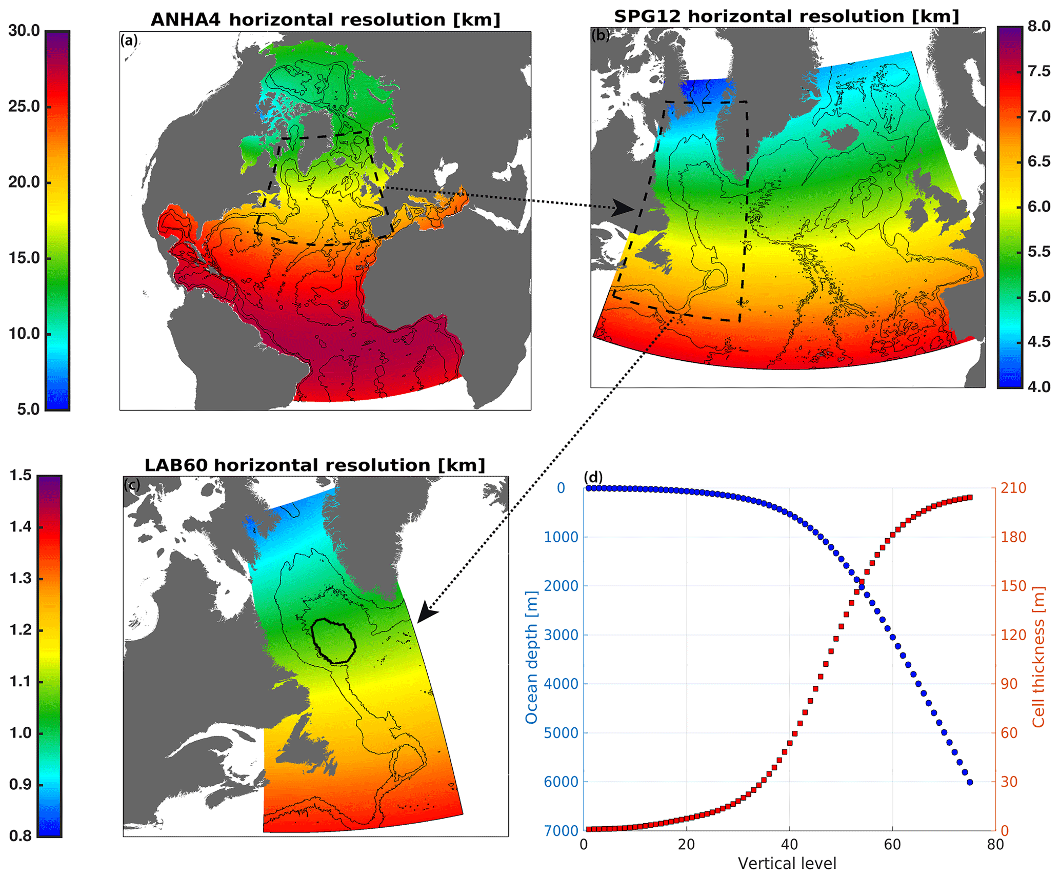
Figure 1Domain setup for the (a) ANHA4 parent domain, (b) the SPG12 nest, and (c) the LAB60 nest. The horizontal grid resolution, in kilometers, is identified by color. All domains share identical vertical grid structure (d). The thick black contour in panel (c) identifies a region of interest where calculations of LSW's density, thickness, and mixed layer depth are determined. The 1000, 3000, and 5000 m isobaths are shown via the thin black contours.
Numerous high-resolution simulations have been carried out within the North Atlantic. VIKING20X (Rieck et al., 2019) and its predecessor VIKING20 are global 1∕4∘ simulations that have a high-resolution 1∕20∘ nest. VIKING20X is a multi-decade simulation that is capable of resolving eddies within the Labrador Sea. However, simulations with a 1∕20∘ horizontal resolution may not resolve sub-mesoscale processes (Su et al., 2018) that can impact stratification by carrying heat and freshwater; thus, a higher resolution is needed. The 1∕50∘ HYCOM (Chassignet and Xu, 2017), 1∕60∘ NATL60 (Fresnay et al., 2018), and eNATL60 (Julien Le Sommer et al., unpublished data) provide great insights into the importance of resolving eddies. However, computational expense with such high-resolution simulations is very high, both in computer time and operational costs. This often forces higher-resolution simulations to have a reduced length (perhaps only a few years). The Labrador Sea experiences significant interannual variability (Fischer et al., 2010), and such short simulations may completely miss any connection between LSW production and changes in the AMOC. As such, any high-resolution simulation that is capable of resolving the fine-scale features within the Labrador Sea should be carried out for many years to further understand the climate system. Resolving the full North Atlantic at high resolution (1∕60∘) and carrying out a simulation for longer than 10 years would currently be extremely expensive; the above 1∕60∘ simulations are 5 or so years in length. However, one can incorporate nested domains to increase horizontal resolution with a relatively minor increase in computational cost.
To simulate the Labrador Sea as accurately as possible, we set up a complex numerical configuration that achieves very high resolution within the Labrador Sea while keeping computational costs low such that we will produce over 15 years of simulated data. This simulation will be kept up to the near present (lagged a few months depending on the availability of forcing data). The high resolution allows for explicit representation of eddies which are crucial to controlling the stratification within the region. We will first describe the model configuration in detail and then compare it with similarly forced lower-resolution simulations to understand how changes in horizontal resolution impact model results in the Labrador Sea.
Table 1Domain settings for the ANHA4 parent domain, the SPG12 nested domain, and the LAB60 nested domain. Other settings that are invariant to the domain are shown in Table 2.

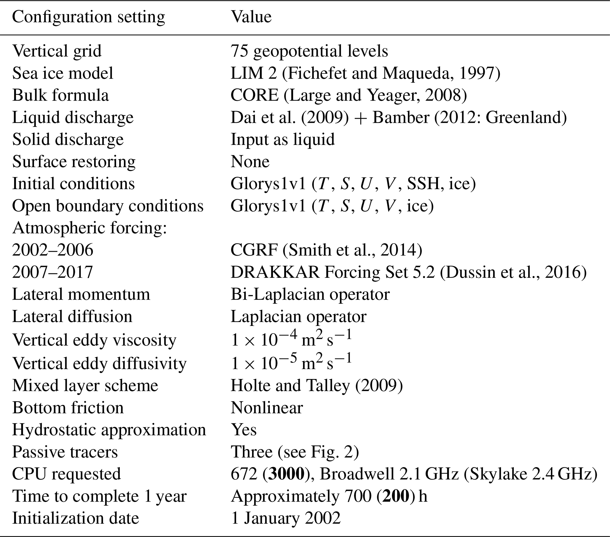
The numerical model used for our high-resolution simulation is the Nucleus for European Modelling of the Ocean (NEMO; Madec, 2008), version 3.6, which is coupled to a sea ice model, LIM2 (Fichefet and Maqueda, 1997). The 1∕4∘ Arctic Northern Hemisphere Atlantic configuration (ANHA4; Fig. 1a) is used and includes a double nest via the Adaptive Grid Refinement in Fortran package (AGRIF; Debreu et al., 2008). The AGRIF software allows for high-resolution nests to communicate along their boundaries, passing information back and forth between domains. The parent ANHA4 domain extends from the Bering Strait, through the Arctic and North Atlantic, to 20∘ S in the South Atlantic. The parent domain's nest uses a spatial and temporal refinement factor of 3, bringing the resolution to 1∕12∘ and the time step to 240 s (Table 1) in the North Atlantic subpolar gyre domain (SPG12; Fig. 1b). An ANHA4 configuration with an SPG12 nest has been evaluated before by investigating how model resolution influences Labrador Sea Water formation (Garcia-Quintana et al., 2019) as well as eddy formation and eddy fluxes in the North Atlantic Current (Müller et al., 2017, 2019). Another nest is implemented within the SPG12 domain, using a spatial and temporal refinement of 5, increasing the horizontal resolution from 1∕12∘ to 1∕60∘ and reducing the time step to 48 s within the Labrador Sea (LAB60; Fig. 1c). All nests allow two-way communication such that the parent domain supplies boundary conditions while the daughter domain returns interpolated values to all associated parent grid points. All domains have different horizontal grid spacing, but they share the same vertical grid which is set to 75 geopotential levels (Fig. 1d) using partial steps (Barnier et al., 2006). This simulation involves three domains (ANHA4, SPG12, and LAB60), although we primarily discuss what occurs within the 1∕60∘ nest.
Table 2Model configuration settings that are identical between all three domains. Bold values indicate values that were changed when we migrated LAB60 from the Graham cluster to Niagara. The abbreviations used in the table are as follows: T is temperature; S is salinity; U and V are the zonal and meridional ocean velocity, respectively; and SSH is the sea surface hight.
A total variance dissipation scheme (Zalesak, 1979) was used in all domains to calculate horizontal advection. A Laplacian operator was used to compute lateral diffusion in all domains, whereas a bi-Laplacian operator was used for lateral momentum mixing. As some model parameters are grid-scale dependent, Table 1 displays these settings. As lateral boundary conditions have been shown to be very important for producing Irminger rings in high-resolution simulations (Rieck et al. 2019), we used no-slip lateral boundary conditions within the LAB60 domain whereas the other domains had free-slip conditions. Model mixed layer depths were calculated via the vertical gradient in temperature and salinity (Holte and Talley, 2009) instead of via a 0.01 kg m−3 change in potential density between the surface and the bottom of the mixed layer; the latter method can produce deeper mixed layers than observations suggest (Courtois et al., 2017). Settings not listed in Table 1 indicate that all domains have an identical value or option; some of these important settings are shown in Table 2.
Model bathymetry was interpolated from the 1∕60∘ ETOPO GEBCO dataset (Amante and Eakins, 2009) to each domain's grid, and bathymetric smoothing was carried out along nest boundaries in order to conserve volume where the parent domain supplies boundary conditions to the daughter domain. All domains were initialized from GLORYS1v1 (Ferry et al., 2010), a global reanalysis ocean simulation, at the beginning of 2002. Monthly open boundary conditions – 3-D T (temperature), S (salinity), U (zonal ocean velocity), V (meridional ocean velocity), and 2-D SSH (sea surface hight) and ice values – across the Bering Strait and 20∘ S were supplied to the ANHA4 domain. These boundary conditions were linearly interpolated from monthly values, overriding the values within the boundary without the use of a sponge layer. Runoff was supplied via Dai et al. (2009), and we also included Greenland runoff as estimated from a surface mass balance model (Bamber et al., 2012). Without an iceberg model functioning with the AGRIF software, we treated all solid runoff as a liquid, thereby capturing the full freshwater mass at the cost of accuracy in the spatial and temporal placement of freshwater emitted from icebergs.
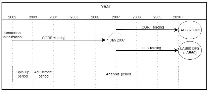
Figure 2Diagram showing the multiple periods of the LAB60 simulation. The original simulation was initialized with CGRF atmospheric forcing in 2002, although a branch swapping to DFS occurred at the start of 2007. This DFS branch is what is primarily presented in this study.
Precipitation, shortwave radiation, downward longwave radiation, 2 m specific humidity, 2 m temperature, and 10 m meridional and 10 m zonal winds originally were supplied from the Canadian Meteorological Centre's Global Deterministic Prediction System's Reforecast product (CGRF; Smith et al., 2014). While the reforecasts had high temporal (hourly) and spatial resolution (33 km in the Labrador Sea), we found the air–sea fluxes were slightly too weak to sustain deep convection after 2010. Rather than completely starting over, we switched the atmospheric forcing in 2007 (Fig. 2) when LAB60's mixed layer was still similar to observations. Starting on 1 January 2007, we used the DRAKKAR Forcing Set 5.2 (DFS; Dussin et al., 2016). DFS supplies data at 3 h increments for wind, temperature, and humidity, whereas precipitation and radiation are daily. DFS has a spatial resolution that is approximately 45 km within the Labrador Sea. Our own analysis of the CGRF data showed a 2002–2015 average yearly heat loss of 47 W m−2 from the interior Labrador Sea, whereas DFS removed 53 W m−2 (Clark Pennelly and Paul G. Myers, personal communication, 2020). Increasing the horizontal resolution likely increased the horizontal buoyancy fluxes and rendered the CGRF's air–sea heat loss, which was appropriate in our ANHA4 and ANHA12 configurations, inadequate. The decision to swap to DFS was based on its greater heat loss, which promotes a better mixed layer depth throughout the Labrador Sea; however, a different forcing product will eventually be needed, as DFS does not currently extend past 2017. Figure S1 in the Supplement depicts the difference in the mixed layer depth between the LAB60 simulation forced by CGRF, when forced with CGRF through 2007 and then forced by DFS, as well as what ARGO observations suggest. The weaker air–sea heat loss as forced by the CGRF product leaves the mixed layer with little interannual variability; this does not compare well with observations.
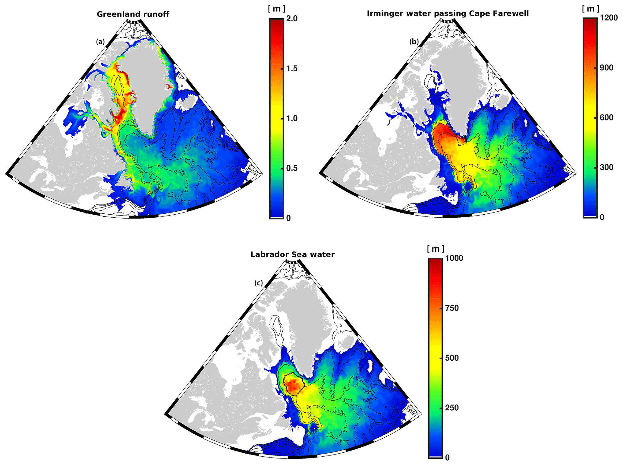
Figure 3The three passive tracers used within our LAB60 simulation with the source regions indicated by thick black lines: (a) Greenland runoff, (b) Irminger Water (T > 3.5 ∘C S > 34.88) that flows west past Cape Farewell, and (c) Labrador Sea Water (σθ > 27.68 kg m−3) produced each convective season. Images are from the simulation date 1 January 2010. Bathymetric contours are every 1000 m. Units are the thickness, in meters, of the tracer. Note that as all three domains are included in this figure, the spatial resolution changes within each subfigure.
Early testing showed that adding passive tracers increases the computational resources required by about 20% per passive tracer. To keep the simulation from requiring too many resources, we limited LAB60 to three passive tracers:
-
liquid runoff from Greenland;
-
Irminger Water (T > 3.5 ∘C, S > 34.88) that flows westward past Cape Farewell (Fig. 3b); and
-
Labrador Sea Water (σθ > 27.68 kg m−3) formed within the mixed layer of the Labrador Sea (Fig. 3c).
Runoff from Greenland was included due to the importance of Greenland's freshwater contribution to changes within the Labrador Sea. Water mass definitions for Irminger Water and Labrador Sea Water were selected based on previous studies (i.e., Kieke et al., 2006; Myers et al., 2007). Note that there is no maximum density criteria given to our Labrador Sea Water tracer – the tracer is formed throughout the water column until it reaches the bottom of the mixed layer. Figure 3 illustrates both the source regions and the tracer extent as of 1 January 2010. Although these water masses have been studied before (Kieke et al., 2006; Myers et al., 2007; Böning et al., 2016), there has been no attempt to use them as passive tracers at a resolution higher than 1∕20∘ (Böning et al., 2016).
The LAB60 simulation originally started on the Graham cluster of Compute Canada. Other high-resolution simulations often use thousands of computer processors, but our simulation could not run on more than 672 CPUs on this cluster as it would stall during domain construction. The years 2002–2007 were carried out on Graham, after which a new allocation on a different high performance Compute Canada cluster, Niagara, became available to us. The LAB60 simulation did not suffer from the same issue on Niagara as it did on Graham, and we were able to use many more processors. Initial testing found a substantial increase in the number of days simulated per job submission when the number of CPUs was increased from 672 to 3000; tests using 4000 CPUs showed no further improvement. Thus, we carried out the remainder of the LAB60 simulation using 3000 CPUs. Each job submission required around 22 h to carry out, providing 40 d of model output. The real time to finish each 40 d submission naturally varied across the year, increasing during winter; this was attributed to the sea ice model.
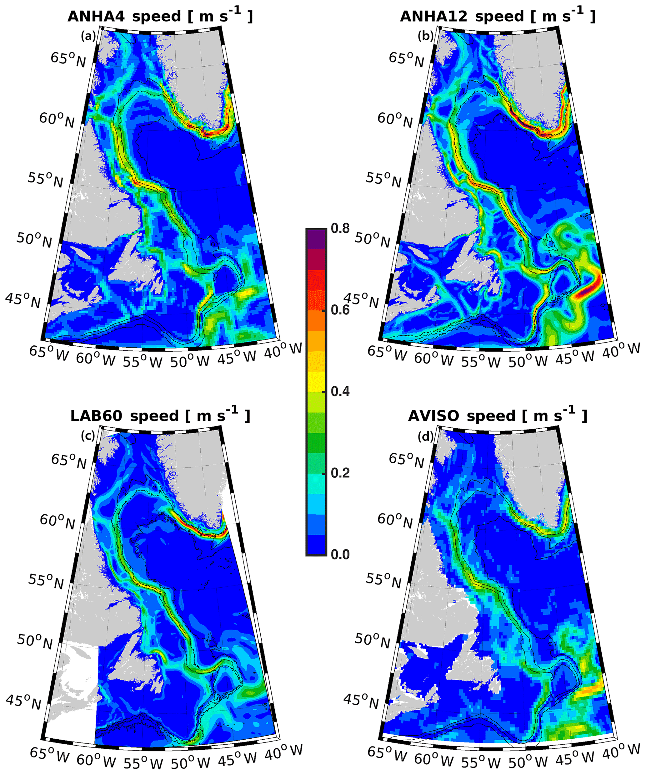
Figure 4Top 50 m average speed (2004–2013) for (a) ANHA4, (b) ANHA12, (c) LAB60, and (d) from AVISO observations. The 1000, 2000, and 3000 m isobaths are shown by the black contour lines.
A spin-up period (Fig. 2) was required as the model quickly became unstable and crashed. We attributed this to the interpolation of the 1∕12∘ GLORYS1v1 data onto the LAB60 grid; the resulting data were not smooth enough and numerical noise was generated, leading to model failure. To reduce this noise, a gradual spin-up procedure took place. First, we kept the numerical time step very low (2 s in LAB60) when the model was initialized. We also set the 1∕60∘ nests' eddy viscosity and diffusivity values to be equal to those within the SPG12 nest. We then gradually increased the time step and reduced the viscosity and diffusivity values over the first year (2002) to the parameter values in Table 1. Other than also increasing the time step to stay in line with LAB60, no other values were changed across the coarser ANHA4 and SPG12 domains. To allow LAB60 to adjust to the final settings, we consider the year 2003 to be an adjustment year (Fig. 2).
To assess the validity of LAB60, model results were compared with AVISO satellite data (https://www.aviso.altimetry.fr/, last access: 9 November 2018), specifically U∕V geostrophic velocities, which are derived from the sea surface height. Argo profiler data (http://www.argo.net/, last access: 6 February 2019) were also used to assess the mixed layer. Bottle data from cruise 18HUD20080520, accessed from CCHDO (https://cchdo.ucsd.edu/cruise/18HU20080520, last access: 10 April 2018) on 10 April 2018 were used to compare observations across the AR7W section.
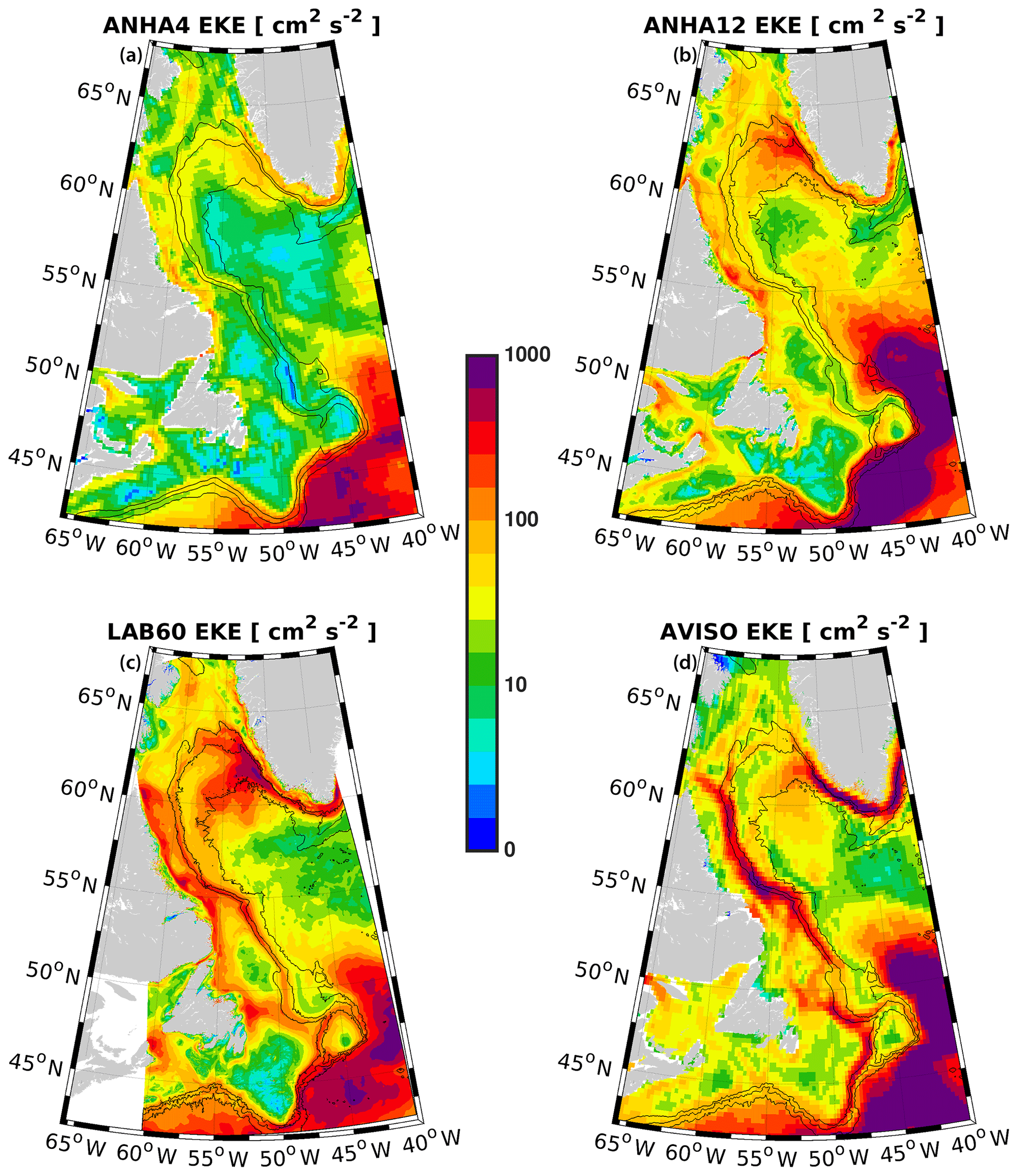
Figure 5Eddy kinetic energy (EKE), as calculated from geostrophic velocities resulting from the sea level height anomaly, are shown for (a) ANHA4, (b) ANHA12, and (c) our LAB60 simulation, from 2004 to 2013. Observations via AVISO are identified in panel (d). The 1000, 2000, and 3000 m isobaths are shown by the black contour lines. A log scale was used for clarity.
To understand what is gained by resolving the Labrador Sea at 1∕60∘, we compare the output of our LAB60 simulation with similarly forced ANHA simulations at both 1∕4∘ (ANHA4) and 1∕12∘ (ANHA12). The large-scale circulation (top 50 m) is shown for our three simulations (Fig. 4) as well as for AVISO geostrophic velocities. All simulations have higher speed within the West Greenland Current (ANHA4: up to 0.8 m s−1; ANHA12: 0.8 m s−1; LAB60: 0.6 m s−1; AVISO: 0.4 m s−1) and the Labrador Current (ANHA4: up to 0.6 m s−1; ANHA12: 0.6 m s−1; LAB60: 0.4 m s−1; AVISO: 0.4 m s−1), as altimetry observations suggest slower speeds here. However, Lin et al. (2018) found a maximum speed of up to 0.74 m s−1 along the west coast of Greenland. Both the ANHA4 and ANHA12 configurations have larger values further up the western coast of Greenland and connecting the West Greenland Current and the Labrador Current; these features do not occur in LAB60 or the observations. As LAB60 and the observations have a lower average speed within these boundary currents, we suspect that all configurations have some large differences in eddy activity, particularly where these boundary currents occur.
Eddy kinetic energy (EKE: ); Fig. 5) was calculated from the geostrophic velocity anomaly based on the sea level anomaly (SLA) from the 2004 to 2013 mean state:
where g is the gravitational constant, f is the Coriolis parameter, and Δy and Δx are model grid length. Overbars indicate the 2004–2013 mean value, and primed variables indicate a deviation from the mean state. AVISO observations were already supplied as geostrophic velocities.
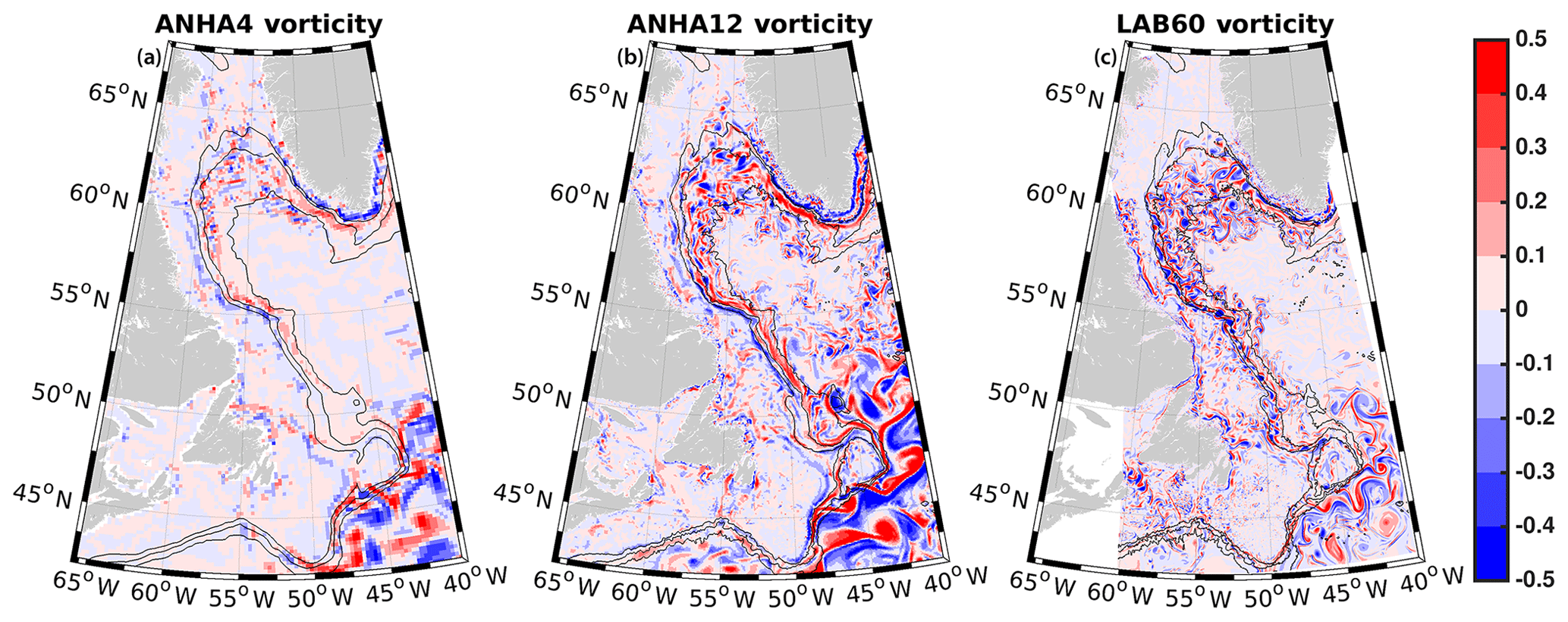
Figure 6Top 50 m relative vorticity, normalized by the planetary vorticity, as simulated by (a) ANHA4, (b) ANHA12, and (c) LAB60 on 16 March 2008. The 1000, 2000, and 3000 m isobaths are shown by the black contour lines.
High EKE levels can be found along the west coast of Greenland (Fig. 5), extending into the interior of the basin around 62∘ N, as well as along the Labrador coast's shelf break. The path extending from the west coast of Greenland is mostly due to Irminger rings which leave this coast and travel westward (Chanut et al., 2008). While the EKE extending from western Greenland enters the interior of the Labrador Sea, the EKE that stems from the Labrador coast does not penetrate far into the interior. The ANHA4 simulation has a low EKE along the west coast of Greenland (around 100 cm2 s−2) and along the Labrador Coast's shelf break (10–30 cm2 s−2). The ANHA12 simulation shows improvement, with a much higher EKE extending from west Greenland (100–300 cm2 s−2); however, the EKE does not quite extend into the interior of the Labrador Sea but instead remains in the northern Labrador Sea. Furthermore, there is additional EKE along the Labrador shelf break (30–50 cm2 s−2) compared with ANHA4. The LAB60 simulation shows further improvement, as the EKE signature from the western Greenland coast is greater (100–1000 cm2 s−2) and now enters into the interior of the Labrador Sea. A notable increase in EKE also occurs along the Labrador shelf break (100–200 cm2 s−2) and within the interior Labrador Sea (10–100 cm2 s−2). LAB60 matches well with observations along the western coast of Greenland and the Labrador shelf break (both above 1000 cm2 s−2) as well as the interior Labrador Sea (10–100 cm2 s−2). LAB60's higher interior EKE may be partially from convective eddies that are formed during the wintertime. However, LAB60 has a lower EKE within the northwest corner, where ANHA4, ANHA12, and the observations exceed 1000 cm2 s−2 over a wide area. LAB60 matches the spatial distribution, albeit with reduced EKE.
The differences in the EKE field between these configurations identify that each simulation is resolving features of varying spatial scales. The ANHA4 simulation, with low EKE within the Labrador Sea, does not adequately resolve eddies in this region, as illustrated by a snapshot of normalized model relative vorticity (Fig. 6). However, the larger-scale meanders within the North Atlantic Current are visible. ANHA12 shows a greater degree of mesoscale features (50 to 500 km), although distinct eddies within the Labrador Sea are also not resolved. LAB60 resolves eddies along both the west coast of Greenland and the Labrador Coast. Video 1 in the Supplement shows LAB60's normalized relative vorticity.
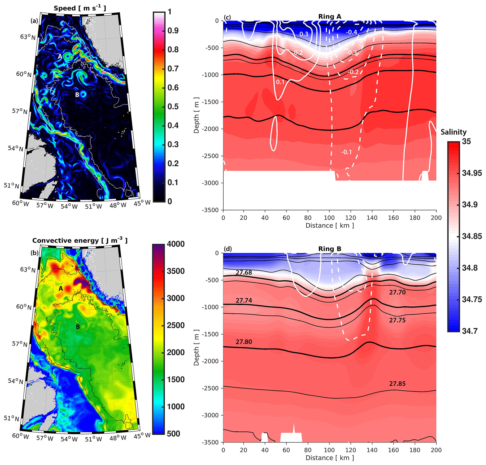
Figure 7LAB60 snapshot (26 July 2007) of the surface speed (a) and convective energy (b) within the Labrador Sea. Two Irminger rings are identified by their age using letters: Ring A is a young Irminger ring, whereas Ring B is comparatively older. An east–west cross section through each of these Irminger rings is shown in panels (c) and (d), respectively, where colors indicate salinity, black contours indicate potential density using a contour interval of 0.05 kg m−3, and white contours indicate meridional velocity where the southern flow is dashed and the northern flow is solid, using a contour interval of 0.1 m s−1. Thick black contours indicate the potential density classification of upper Labrador Sea Water (σθ = 27.68 to 27.74 kg m−3) and classical Labrador Sea Water (σθ = 27.74 to 27.80 kg m−3).
A few Irminger rings are shown in Fig. 7, which provides a snapshot in time from 26 July 2007. A newly spawned ring (Fig. 7c) shows very strong surface speeds (up 0.6 m s−1 for Ring A; Fig. 7a), whereas older eddies to the south have reduced speeds (up to 0.3 m s−1 for Ring B; Fig. 7a). To investigate the stratification strength, we calculate the amount of energy needed to produce a neutrally stratified column extending down to some reference depth, h. This proxy, called convective energy, is given by the following equation:
where g is the gravitational constant; Area is the total surface area over our region of interest (Fig. 1c); h is the reference depth (2000 m used in this study); ρθ(z) and ρθ(h) are the potential density at each grid cell and the potential density of the grid cell at the reference depth, respectively; and A is the surface area of each grid cell. A strongly stratified column of water corresponds to a high convective energy value. A snapshot of convective energy (Fig. 7b) shows that most of these eddies have substantially higher values compared with the background Labrador Sea, suggesting that the cool and fresh WGC water and the warm and salty Irminger Water keep these eddies strongly stratified. However, these eddies age within the Labrador Sea, and while a new eddy has strong stratification (> 3000 J m−3), an eddy that has evolved over many months (Fig. 7d) has weaker stratification (about 2000 J m−3). Older eddies may have very weak stratification as they may have experienced two convective winter periods of buoyancy removal. This has been noted before, as Lilly et al. (2003) found aged Irminger rings with a mixed layer that surpassed 1000 m.

Figure 8Convective energy (CE), the strength of stratification down to a reference depth of 2000 m, is shown for (a) ANHA4, (b) ANHA12, and (c) LAB60. Convective energy was averaged from 2004 to 2013. Values where the depth of the seafloor was less than 2000 m were removed to preserve clarity. Bathymetric contours (black lines) are shown every 500 m.
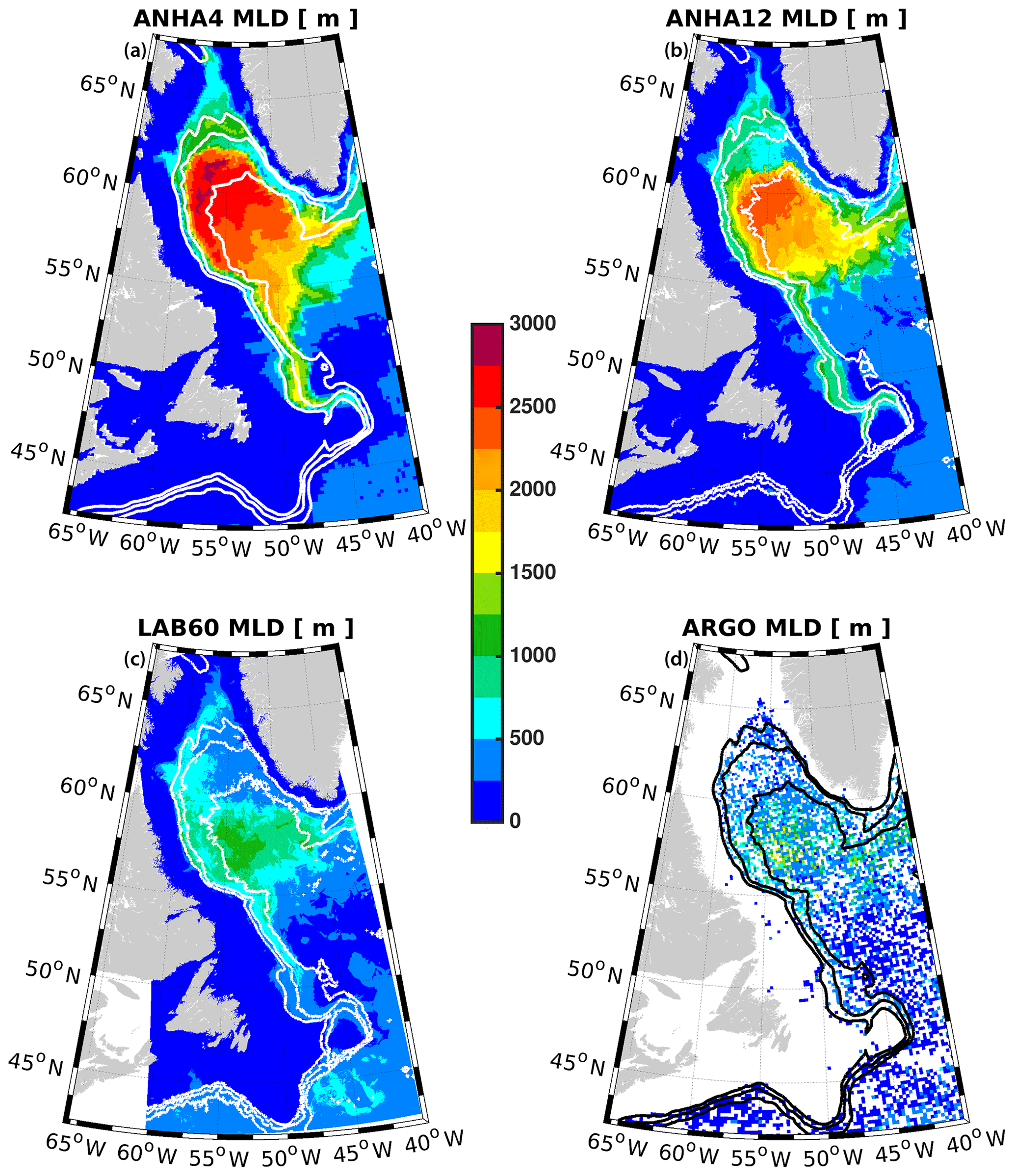
Figure 9Maximum mixed layer depth for (a) ANHA4, (b) ANHA12, (c) LAB60, and (d) ARGO observations, where available, from 2004 through to the end of 2013. For clarity, the ARGO data were placed on the same grid as ANHA4. The 1000, 2000, and 3000 m isobaths are shown using the white and black contours
These differences in resolving the mesoscale (50 to 500 km) and sub-mesoscale (< 50 km) processes within each simulation produced significant changes within the Labrador Sea, as seen from modeled convective energy values averaged from 2004 to 2013 (Fig. 8). Resolving few eddies, the ANHA4 simulation's interior Labrador Sea lacks the buoyancy flux and remains very weakly stratified across a wide region. The ANHA12 simulation partially resolves some mesoscale features and eddy fluxes from the Greenland coast, which supplies buoyancy to the Northern Labrador Sea and has higher convective energy. Furthermore, the spatial extent of the weakly stratified region has shrunk and resides primarily within the Labrador Sea, as opposed to ANHA4 which spills out of the basin. LAB60, which is fully capable of resolving buoyant eddies from the Greenland and Labrador coast, as well as convective eddies, has a much stronger degree of stratification in the interior region. A visible path of strong stratification appears around 60∘ N along this coastline, eventually extending away from the coastline around 62∘ N. This path is consistent with the general path that simulated Irminger rings take (Chanut et al., 2008). Video 2 in the Supplement shows the convective energy of the LAB60 simulation from 2004 through to the end of 2013.
The ANHA4 simulation experiences weaker stratification in the Labrador Sea than ANHA12 and LAB60, driving a deeper maximum mixed layer that also covers a larger spatial extent (Fig. 9). However, the maximum mixed layer depth as simulated by ANHA4 and ANHA12 greatly exceed what Argo observations suggest (Fig. 9d). ANHA12 has higher EKE within the WGC, supplying more buoyancy to the northern portion of the Labrador Sea, reducing both the vertical extent of the mixed layer and the spatial extent where the mixed layer is deeper than 1000 m. LAB60 has higher EKE than ANHA12, and the vertical and spatial extent of deep mixing is reduced even further. LAB60's mixed layer is far more similar to what ARGO observations imply, suggesting that the additional eddy fluxes are fairly accurate. The evolution of LAB60's mixed layer depth is shown in Video 3 in the Supplement from 2004 through to the end of 2013.
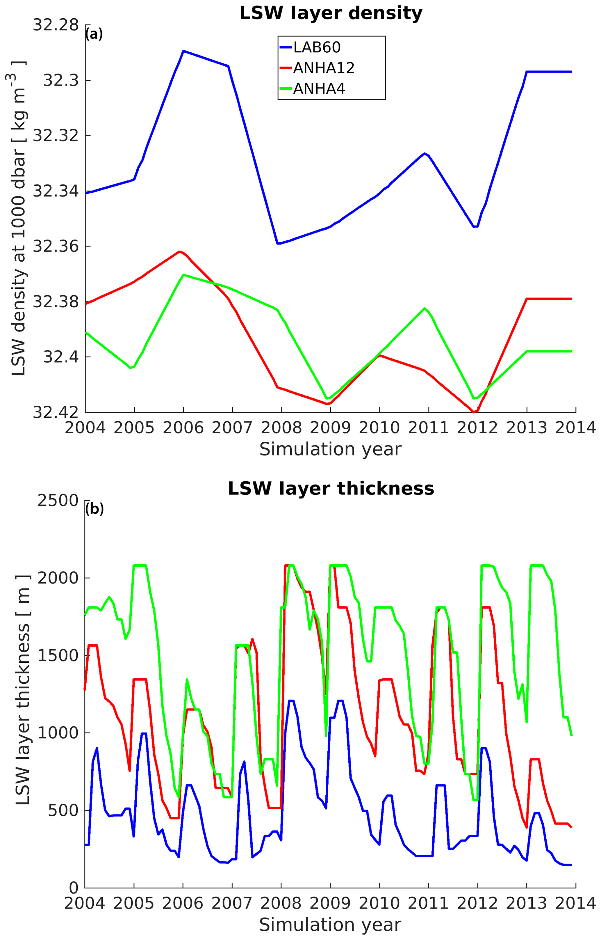
Figure 10Labrador Sea Water (LSW) density (a) and thickness (b) for the LAB60, ANHA12, and ANHA4 configurations. LSW density was determined from the thickest layer where a 0.001 kg m−3 change in potential density (ref: 1000 dbar) occurred within the black polygon outlines in Fig. 1c. The LSW layer was then calculated between this density and one that was 0.02 kg m−3 less dense.
After the bottom of the mixed layer returns to the near surface, a newly formed LSW mass is left behind. To account for density drift, we allow the LSW classification to evolve in time, unlike our LSW passive tracer. We calculated LSW density and thickness by binning by the potential density, referenced to 1000 dbar, with bin lengths of 0.001 kg m−3. This was carried out within the black outlined polygon in Fig. 1c for each daily output file per year. The density bin that had the thickest layer across the year was set as the maximum density of LSW for that year. The minimum density was set to be 0.02 kg m−3 less than the maximum density. Linear interpolation occurred between years to allow for a gradual shift in density to prevent staircase patterns from emerging. Large differences in both the density and the thickness are present between the simulations shown in Fig. 10. The ANHA4 and ANHA12 simulations have similar density values of LSW, whereas the LAB60 simulation is less dense. While the interannual variability matches fairly well across all configurations, the density values suggested by LAB60 are closer to ARGO observations (32.34 to 32.36 kg m−3; Yashayaev and Loder, 2016) during the same time period. We suspect that the denser LSW formed by ANHA4 and ANHA12 is primarily attributed to the lack of buoyancy coming from Greenland. As similar air–sea heat losses should occur in all three configurations, the weaker stratification of ANHA4 and ANHA12 indicates that deep mixing is more likely producing not only a denser LSW layer but also a thicker one. Yashayaev and Loder (2016) also investigated the thickness of LSW (their Fig. 8), and while our simulations do not quite capture the same interannual variability and amplitude suggested in their analysis using ARGO profilers, LAB60 is far more accurate than the lower-resolution configurations.
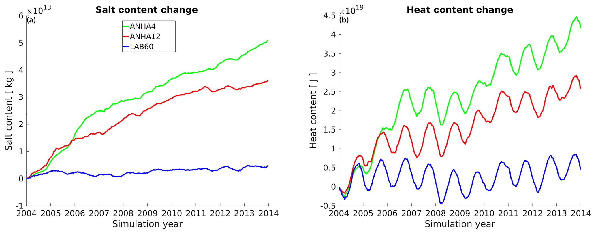
Figure 11Numerical salt (a) and heat (b) drift in our three simulations as they evolve from 1 January 2004. The salt and heat content is calculated over the full ocean column within the polygon in Fig. 1c.
All simulations encounter some degree of numerical drift within the Labrador Sea (Fig. 11), judging from the salt and heat content change as calculated between the surface and seafloor within the polygon in Fig. 1 from 2004. ANHA4 experiences the largest drift in both salt and heat, helping us to understand why LSW is so dense in this simulation. ANHA12 also experiences drift, although it is slightly less severe. LAB60 has a small but gradual increase in both salt and heat content, although it is difficult to state if this is drift or simply interannual to decadal variability. Regardless of the cause, LAB60's change in both heat and salt content is very minimal compared with the lower-resolution simulations.
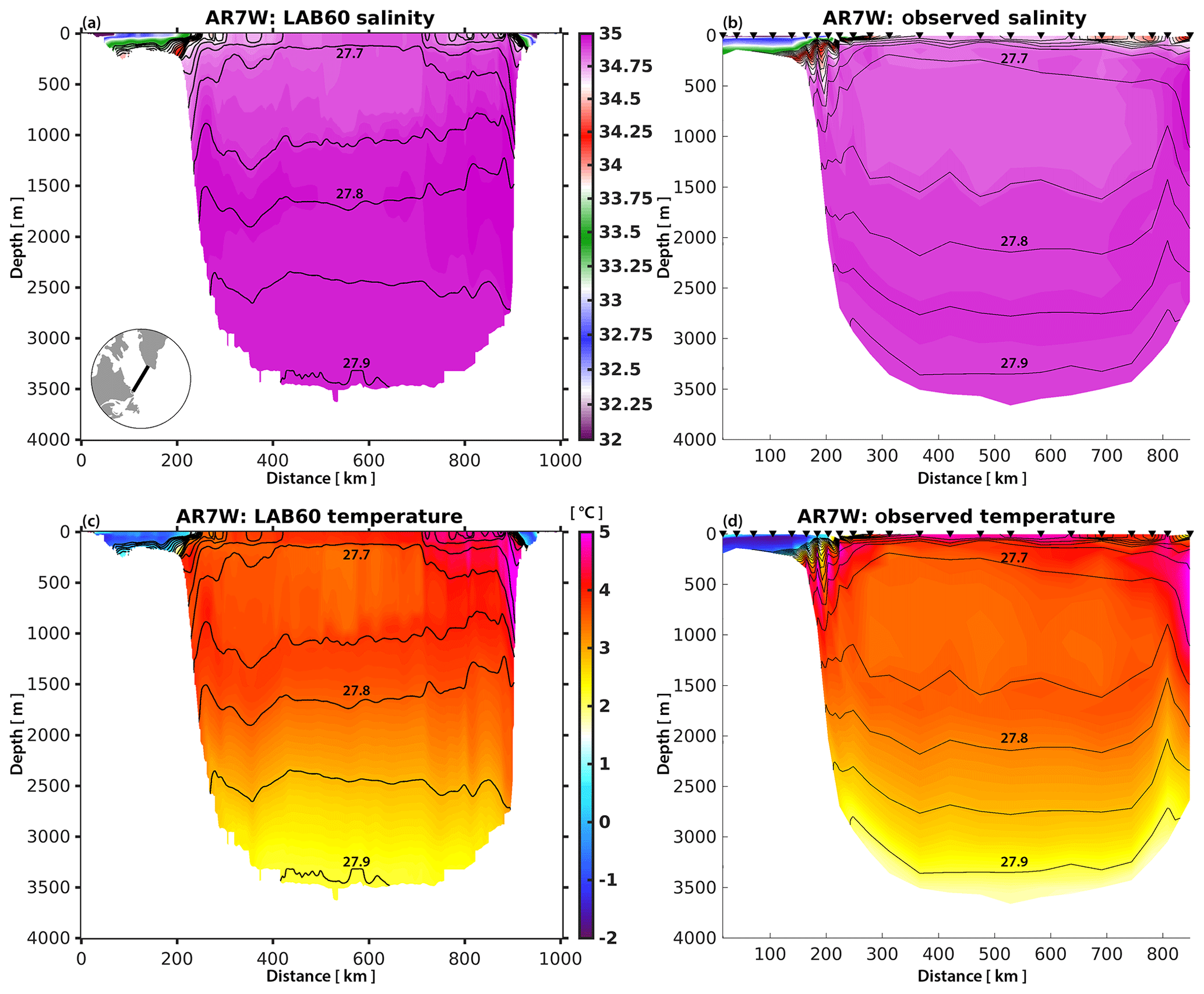
Figure 12Salinity (a, b) and temperature (c, d) section across AR7W as determined by the LAB60 simulation (a, c) and observations (b, d) from May 2008. Downward triangles identify collection sites across the AR7W transit carried out by the CCGS Hudson. The potential density (black contours) isopycnal interval is 0.05 kg m−3.
When compared with bottle data collected during a single hydrographic cruise across Atlantic Repeat Hydrography Line 7 West (AR7W; Fig. 12), LAB60 is slightly warmer (about 0.25 ∘C) and saltier (about 0.05 kg m−3) throughout the interior. This causes LAB60 to be slightly denser with isopycnals residing higher than observations during this cruise suggest. Observations were not carried out above Greenland's continental slope, although they show some presence of the warm core of the WGC which the model captures. Salinity values close to the Labrador coast compare well, whereas LAB60 is slightly warmer (about 0.5 ∘C) above the continental shelf.
The three passive tracers implemented within the full LAB60 configuration (Fig. 3) show where Greenland runoff, Irminger Water, and Labrador Sea Water travel to. These tracers were selected because they either contain a significant amount of buoyant water compared with the Labrador Sea or are produced via convection in the Labrador Sea. From this image on 1 January 2010, we see that a large portion of Greenland's runoff (Fig. 3a) resides within Baffin Bay and along the Labrador Coast. Some of this tracer is present where the ocean depth is greater than 2000 m. A few Irminger rings are identifiable, due to their thicker freshwater cap, in water deeper than 3000 m. Little exchange with the interior basin appears to occur along the Labrador Current until the vicinity of Flemish Cap, after which a significant portion of the tracer propagates eastward. Video 4 in the Supplement shows the evolution of this tracer from 2004 through to the end of 2013.
Irminger Water (T > 3.5 ∘C, S > 34.88; Fig. 3b), which flows west past Cape Farewell, enters the interior Labrador Sea in the greatest amounts where the seafloor is at a depth between 2000 and 3000 m. Similar to the findings above, individual Irminger rings are visible and contain a larger amount of Irminger Water than the surrounding water. This water mass also flows along the Labrador Coast until it is in the vicinity of Flemish Cap. Video 5 in the Supplement shows the evolution of this tracer from 2004 through the end of 2013.
Our Labrador Sea Water tracer (Fig. 3c) is traced where the mixed layer produces water with a potential density above 1027.68 kg m−3 within the black contour identified in the figure. This definition differs from our method of classifying LSW, as we did not implement any Fortran code to detect and compensate for density drift in our simulation and instead stuck to a strict density classification for this tracer. As this image was made at the start of the convection season, the current deep patch is a freshly produced layer that reaches a depth of up to 800 m. After forming, LSW spreads southward along the Labrador shelf break as well as to the southeast. Video 6 in the Supplement shows the evolution of this tracer from 2004 through to the end of 2013.
We describe a more than 10-year-long, high-resolution simulation that achieves a 1∕60∘ horizontal resolution in the Labrador Sea via two nests inside a regional configuration, resolving mesoscale and sub-mesoscale processes that strongly impact the deep convection which occurs here. We show that lower-resolution simulations fail to resolve the key processes that strongly control the production of Labrador Sea Water, which is an important water mass within the Atlantic Meridional Overturning Circulation. While the NATL60 and eNATL60 simulations were designed with the Surface Water and Ocean Topography (SWOT) altimetry satellite mission in mind (NATL60 website: https://meom-group.github.io/swot-natl60/virtual-ocean.html, last access: 14 October 2020), their integration period, like many other high-resolution simulations, is a handful of years. LAB60, although covering a much smaller region, could be a valuable asset to many users who require a lengthy period of high-resolution model output. We have also included three passive tracers that are often excluded in simulations at this resolution. Our three passive tracers highlight regions where each water mass enters the interior region of the Labrador Sea, demonstrating the pathways of buoyant Greenland melt and Irminger Water. Furthermore, we trace Labrador Sea Water, which is formed during the convective winter period.
We show that LAB60 has greater EKE than our lower-resolution simulation, resolving eddy fluxes including Irminger rings, boundary current eddies, and likely convective eddies as indicated by greater EKE within the interior. Boundary current eddies still appear relatively disconnected from the interior basin, adding further support to the fact that these eddies have limited influence on convection and restratification (Rieck et al., 2019). We offer no additional support regarding the relative importance of Irminger rings and convective eddies on controlling deep convection; this is currently being investigated for a later publication. Model drift appears to be very low, which is a large improvement over the ANHA4 and ANHA12 configurations. The drift might produce slightly denser LSW than the observations suggest; however, LAB60's density is much more accurate than ANHA4 and ANHA12. The boundaries of LAB60, supplied by the inner SPG12 nest, may influence the high-resolution nest. We note that the North Atlantic Current, which is close to the boundary, has less EKE and vorticity than the ANHA4 and ANHA12 simulations. Conversely, the WGC close to the eastern nested boundary has multiple jets that have been noted in hydrographic data (Robert Pickart, personal communication, 2020). Boundary communication is always a concern in nested simulations, and LAB60 is no different. More investigation will reveal any potential boundary issues, but our results indicate no further areas of potential concern thus far.
Others have investigated the Labrador Sea using numerical simulations with different resolutions. Böning et al. (2016) traced Greenland meltwater with the 1∕20∘ VIKING20 and 1∕4∘ ORCA025 simulations, noting that more meltwater entered the interior Labrador Sea at a higher resolution partially as a result of greater WGC eddy fluxes but not from the Labrador coast. The minor amount of eddy fluxes from the Labrador coast has been previously noted, even at lower resolution (1/3∘; Myers, 2005). Steadily increasing horizontal resolution has not changed this for the Labrador coast so far, although the opposite is true for the WGC. LAB60 shows a clear increase in EKE and likely greater eddy fluxes from the WGC into the interior of the Labrador Sea.
We have many ambitious research topics that we plan to use LAB60 to investigate. This includes (but is not limited to) the variability and structure of the West Greenland Coastal Current, Labrador Sea Water production, and the role of both Irminger rings and convective eddies in controlling stratification in the Labrador Sea. This lengthy high-resolution simulation with three passive tracers will provide valuable information for many numerical studies within the Labrador Sea for years to come.
The Fortran code used to carry out the LAB60 simulation can be accessed from the NEMO version 3.6 repository (https://forge.ipsl.jussieu.fr/nemo/browser/NEMO/releases/release-3.6, last access: 14 October 2020). A few Fortran files were modified to handle our passive tracers. The complete Fortran files as well as the CPP keys, namelists, and associated files can be found on Zenodo (https://doi.org/10.5281/zenodo.3762748, Pennelly, 2020). The initial and boundary conditions, atmospheric forcing, and numerical output were too large to host on a repository and are instead hosted on our lab's servers as well as the Compute Canada Niagara server. These data can be obtained upon request from the corresponding author.
All videos were made by Clark Pennelly in 2020. The DOIs and titles are given below. All videos are hosted by ERA (Education and Research Archive) at the University of Alberta.
Supplemental Video 1: normalized relative vorticity of the LAB60 simulation, from 1 January 2004 through 31 December 2013. Note that a few days are missing due to corrupted output files. DOI: https://doi.org/10.7939/r3-2yts-nw62 (Pennelly and Myers, 2020a).
Supplemental Video 2: convective energy of the LAB60 simulation, with a reference depth of 2000 m. Video takes place from 1 January 2004 through 31 December 2013. Units are in joules per cubic meter (J m−3). Note that a few days are missing due to corrupted output files. DOI: https://doi.org/10.7939/r3-nen0-g831 (Pennelly and Myers, 2020b).
Supplemental Video 3: mixed layer depth (MLD), in meters, of the LAB60 simulation from 1 January 2004 through 31 December 2013. A red contour line shows where the ice concentration is 10 %. A black contour line shows where the MLD exceeds 1000 m. Note that a few days are missing due to corrupted output files. DOI: https://doi.org/10.7939/r3-m6rk-h867 (Pennelly and Myers, 2020c).
Supplemental Video 4: Greenland melt passive tracer, in meters, of the LAB60 simulation. Video takes place from 1 January 2004 though 31 December 2013. Note that a few days are missing due to corrupted output files. DOI: https://doi.org/10.7939/r3-43mg-db88 (Pennelly and Myers, 2020d).
Supplemental Video 5: Irminger Water passive tracer, in meters, of the LAB60 simulation. Video takes place from 1 January 2004 through 31 December 2013. Note that a few days are missing due to corrupted output files. DOI: https://doi.org/10.7939/r3-zwkr-0w35 (Pennelly and Myers, 2020e).
Supplemental Video 6: Labrador Sea Water tracer, in meters, of the LAB60 simulation. Video takes place from 1 January 2004 through 31 December 2013. Note that a few days are missing due to corrupted output files. DOI: https://doi.org/10.7939/r3-7295-ks15 (Pennelly and Myers, 2020f).
The supplement related to this article is available online at: https://doi.org/10.5194/gmd-13-4959-2020-supplement.
PM designed the layout of the LAB60 configuration, which included the region of interest, the numerical length, and the forcing and initial conditions supplied, and supervised CP. CP produced the configuration, modified the Fortran code, set up the configuration on the high-performance computing systems, carried out the simulation, and performed the analysis. The paper was prepared by CP with contributions from PM.
The authors declare that they have no conflict of interest.
The authors would like to thank the NEMO development team and the DRAKKAR group for providing the model code and continuous guidance. We express our thanks to WestGrid and Compute Canada (http://www.computecanada.ca, last access: 14 October 2020) for the computational resources used to carry out our numerical simulations and for archiving the experiments. We would like to thank Nathan Grivault for his help with migrating our configuration between computing clusters and Charlene Feucher for her help with ARGO data.
This research has been supported by the Natural Sciences and Engineering Research Council of Canada (grant nos. RGPCC 433898 and RGPIN 04357).
This paper was edited by Qiang Wang and reviewed by Jan Klaus Rieck and one anonymous referee.
Amante, C. and Eakins, B. W.: ETOPO1 1 Arc-minute global relief model: procedures data sources and analysis. NOAA Technical Memorandum NESDIS, NGDC-24 19, National Oceananic and Atmospheric Administration, Boulder Colorado, USA, 2009.
Bamber, J., van den Broeke, M., Ettema, J., Lenaerts, J., and Rignot, E.: Recent large increases in freshwater fluxes from Greenland into the North Atlantic, Geophys. Res. Lett., 39, 19, https://doi.org/10.1029/2012GL052552, 2012.
Barnier, B., Madec, G., Penduff, T., Molines, J-M., Treguier, A-M., Le Sommer, J., Beckmann, A., Biastoch, A., Böning, C., Dengg, J., Derval, C., Durand, E., Gulev, S., Remy, R., Talandier, C., Theetten, S., Maltrud, M., Mcclean, J., and De Cuevas, B.: Impact of partial steps and momentum advection schemes in a global ocean circulation model at eddy permitting resolution, Ocean Dynam., 56, 543–567, 2006.
Böning, C. W., Behrens, E., Biastoch, A., Getzlaff, K., and Bamber, J. L.: Emerging impact of Greenland meltwater on deepwater formation in the North Atlantic Ocean, Nat. Geosci., 97, 523–528, https://doi.org/10.1038/ngeo2740, 2016.
Bryden, H. L., Longworth, H. R., and Cunningham, S. A.: Slowing of the Atlantic meridional overturning circulation at 25∘ N, Nature, 438, 655–657, https://doi.org/10.1038/nature04385, 2005.
Cael, B. B. and Jansen, M. F.: On freshwater fluxes and the Atlantic meridional overturning circulation, Limnol. Oceanogr., 5, 185–192, 2020.
Chanut, J., Barnier, B., Large, W., Debreu, L., Penduff, T., Molines, J. M., and Mathiot, P.: Mesoscale eddies in the Labrador Sea and their contribution to convection and restratification, J. Phys. Oceanogr., 28, 1617–1643, 2008.
Chassignet, E. P. and Xu, X.: Impact of horizontal resolution (1∕12 to 1∕50) on Gulf Stream separation, penetration, and variability, J. Phys. Oceanogr., 47, 1999–2021, 2017.
Courtois, P., Hu, X., Pennelly, C., Spence, P., and Myers, P. G.: Mixed layer depth calculation in deep convection regions in ocean numerical models, Ocean Model., 120, 60–78, 2017.
Cuny, J., Rhines, P. B., and Kwok, R.: Davis Strait volume, freshwater and heat fluxes, Deep-Sea Res. Pt. I, 52.3, 519–542, 2005.
Curry, B., Lee, C. M., and Petrie, B.: Volume, freshwater, and heat fluxes through Davis Strait, 2004–05, J. Phys. Oceanogr., 41, 429–436, 2011.
Curry, B., Lee, C. M., Petrie, B., Moritz, R. E., and Kwok, R.: Multiyear volume, liquid freshwater, and sea ice transports through Davis Strait, 2004–10, J. Phys. Oceanogr., 44, 1244–1266, 2014.
Dai, A., Qian, T., Trenberth, K. E., and Milliman, J. D.: Changes in continental freshwater discharge from 1948 to 2004, J. Climate, 22, 2773–2792, 2009.
Debreu, L., Vouland, C., and Blayo, E.: AGRIF: Adaptive grid refinement in Fortran, Comput. Geosci., 34, 8–13, 2008.
De Jong, M. F., Bower, A. S., and Furey, H. H.: Seasonal and interannual variations of Irminger Ring formation and boundary-interior heat exchange, J. Phys. Oceanogr., 46, 1717–1734, 2016.
De Steur, L., Hansen, E., Gerdes, R., Karcher, M., Fahrbach, E., and Holfort, J.: Freshwater fluxes in the East Greenland Current: A decade of observations, Geophys. Res. Lett., 36, 23, https://doi.org/10.1029/2009GL041278, 2009.
Dussin, R., Barnier, B., and Brodeau, L.: The making of Drakkar forcing set DFS5, LGGE, Grenoble, France, 2016.
Ferry, N., Parent, L., Garric, G., Barnier, B., and Jourdain, N. C.: Mercator global eddy permitting ocean reanalysis GLORYS1V1: Description and results, Mercator – Ocean Quarterly Newsletter, 36, 15–27, 2010.
Fichefet, T. and Maqueda, M. A. M.: Sensitivity of a global sea ice model to the treatment of ice thermodynamics and dynamics, J. Geophys. Res.-Oceans, 102, 12609–12646, 1997.
Fischer, J., Visbek, M., Zantopp, R., and Nunes, N.: Interannual to decadal variability of outflow from the Labrador Sea, Geophys. Res. Lett., 37, 24, https://doi.org/10.1029/2010GL045321, 2010.
Frajka-Williams, E., Rhines, P. B., and Eriksen, C. C.: Horizontal stratification during deep convection in the Labrador Sea, J. Phys. Oceanogr., 44, 220–228, 2014.
Fratantoni, P. S. and Pickart, R. S.: The Western North Atlantic Shelfbreak Current System in Summer, J. Phys. Oceanogr., 37, 2509–2533, 2007.
Fresnay, S., Ponte, A. L., Le Gentil, S., and Le Sommer, J.: Reconstruction of the 3-D dynamics from surface variable in a high-resolution simulation of the North Atlantic, J. Geophys. Res.-Oceans, 123, 1612–1630, 2018.
Garcia-Quintana, Y., Courtois, P., Hu, X., Pennelly, C., Kieke, D., and Myers, P. G.: Sensitivity of Labrador Sea Water formation to changes in model resolution, atmospheric forcing, and freshwater input, J. Geophys. Res.-Oceans, 124, 2126–2152, 2019.
Gelderloos, R., Katsman, C. A., and Drijfhout, S. S.: Assessing the roles of three eddy types in restratifying the Labrador Sea after deep convection, J. Phys. Oceanogr., 41, 2102–2119, 2011.
Hátún, H., Eriksen, C. C., and Rhines, P. B.: Buoyant eddies entering the Labrador Sea observed with gliders and altimetry, J. Phys. Oceanogr., 37, 2838–2854, 2007.
Holte, J. and Talley, L.: A new algorithm for finding mixed layer depths with applications to Argo data and Subantarctic Mode Water formation, J. Atmos. Ocean. Tech., 26, 1920–1939, 2009.
Kieke, D., Rhein, M., Stramma, L., Smethie, W., LeBel, D. A., and Zenk, W.: Changes in the CFC inventories and formation rates of Upper Labrador Sea Water, 1997–2001, J. Phys. Oceanogr., 36, 64–86, 2006.
Kieke, D., Klein, B., Stramma, L., Rhein, M., and Koltermann, K. P.: Variability and propagation of Labrador Sea Water in the southern subpolar North Atlantic, Deep-Sea Res. Pt. I, 56, 1656–1674, 2009.
Lab Sea Group: The Labrador Sea deep convection experiment, B. Am. Meteorol. Soc., 79, 2033–2058, 1998.
Large, W. G. and Yeager, S. G.: The global climatology of an interannually varying air-sea flux data set, Clim. Dynam., 33, 341–364, 2008.
Latif, M., Roechner, E., Mikolajewicz, U., and Voss, R.: Tropical stabilization of the thermohaline circulation in a greenhouse warming simulation, J. Climate, 13, 1809–1813, 2000.
Lazier, J. R. N. and Wright, D. G.: Annual velocity variations in the Labrador Current, J. Phys. Oceanogr., 23, 659–678, 1993.
Lilly, J. M., Rhines, P. B., Visbeck, M., Davis, R., Lazier, J. R. N., Schott, F., and Farmer, D.: Observing deep convection in the Labrador Sea during winter 1994/95, J. Phys. Oceanogr., 29, 2065–2098, 1999.
Lilly, J. M., Rhines, P. B., Schott, F., Lavender, K., Lazier, J., Send, U., and D'Asaro, E.: Observations of the Labrador Sea eddy field, Prog. Oceanogr., 59, 75–176, 2003.
Lin, P., Pickart, R. S., Torres, D. J., and Pacini, A.: Evolution of the freshwater coastal current at the southern tip of Greenland, J. Phys. Oceanogr., 48, 2127–2140. 2018.
Madec, G.: Note du Pôle de modélisation, Institut Pierre-Simon Laplace (IPSL), France, No 27, ISSN No 1288–1619, 2008.
Marshall, J. and Schott, F.: Open-ocean convection: Observations, theory, and models, Rev. Geophys., 37, 1–64, 1999.
Marzocchi, A., Hurshi, J. J. M., Holiday, N. P., Cunningham, S. A., Blaker, A. T., and Coward, A. C.: The North Atlantic subpolar circulation in an eddy-resolving global ocean model, J. Marine Syst., 142, 126–143, 2015.
McGeehan, I. and Maslowski, W.: Impact of shelf-basin freshwater transport on deep convection in the western Labrador Sea, J. Phys. Oceanogr., 41, 2187–2210, 2011.
Müller, V., Kieke, D., Myers, P. G., Pennelly, C., and Mertens, C.: Temperature flux carried by individual eddies across 47∘ in the Atlantic Ocean, J. Geophys. Res.-Oceans, 122, 2441–2464, 2017.
Müller, V., Kieke, D., Myers, P. G., Pennelly, C., Steinfeldt, R., and Stendardo, I.: Heat and freshwater transport by mesoscale eddies in the southern subpolar North Atlantic, J. Geophys. Res.-Oceans, 124, 5565–5585, 2019.
Myers, P.: Impact of freshwater from the Canadian Arctic Archipelago on Labrador Sea water formation, Geophys. Res. Lett., 32, 6, https://doi.org/10.1029/2004GL022082, 2005.
Myers, P. G., Josey, S. A., Wheler, B., and Kulan, N.: Interdecadal variability in Labrador Sea precipitation minus evaporation and salinity, Prog. Oceanogr., 73, 341–357, 2007.
Pennelly, C.: A 1∕60 degree NEMO configuration within the Labrador Sea: LAB60, Zenodo, https://doi.org/10.5281/zenodo.3762748, 2020.
Pennelly, C. and Myers, P. G.: Relative vorticity of the LAB60 ocean sea-ice simulation: 2004-2013, ERA, https://doi.org/10.7939/r3-2yts-nw62, 2020a.
Pennelly, C. and Myers, P. G.: Stratification strength of the LAB60 ocean sea-ice simulation: 2004-2013, ERA, https://doi.org/10.7939/r3-nen0-g831, 2020b.
Pennelly, C. and Myers, P. G.: Mixed layer depth of the LAB60 ocean sea-ice simulation: 2004-2013, ERA, https://doi.org/10.7939/r3-m6rk-h867, 2020c.
Pennelly, C. and Myers, P. G.: Greenland runoff tracer of the LAB60 ocean sea-ice simulation: 2004-2013, ERA, https://doi.org/10.7939/r3-43mg-db88, 2020d.
Pennelly, C. and Myers, P. G.: Irminger Water tracer of the LAB60 ocean sea-ice simulation: 2004-2013, ERA, https://doi.org/10.7939/r3-zwkr-0w35, 2020e.
Pennelly, C. and Myers, P. G.: Labrador Sea Water tracer of the LAB60 ocean sea-ice simulation: 2004-2013, ERA, https://doi.org/10.7939/r3-7295-ks15, 2020f.
Pennelly, C. Hu, X., and Myers, P. G.: Cross-isobath freshwater exchange within the North Atlantic Subpolar Gyre, J. Geophys. Res.-Oceans, 124, 6831–6853, 2019.
Rattan, S., Myers, P. G., Treguier, A. M., Theetten, S., Biastoch, A., and Böning, C.: Towards an understanding of Labrador Sea salinity drift in eddy-permitting simulations, Ocean Model., 35, 77–88, 2010.
Rieck, J. K., Böning, C. W., and Getzlaff, K.: The nature of eddy kinetic energy in the Labrador Sea: Different types of mesoscale eddies, their temporal variability, and impact on deep convection, J. Phys. Oceanogr., 49, 2075–2094, 2019.
Schmidt, S. and Send, U.: Origin and composition of seasonal Labrador Sea freshwater, J. Phys. Oceanogr., 37, 1445–1454, 2007.
Schulze, L. M., Pickart, R. S., and Moore, G. W. K.: Atmospheric forcing during active convection in the Labrador Sea and its impact on mixed-layer-depths, J. Geophys. Res.-Oceans, 121, 6978–6992, 2016.
Smith, G. C., Roy, F., Mann, P., Dupont, F., Brasnett, B., Lemieux, J. F., Laroche, S., and Bélair, S.: A new atmospheric dataset for forcing ice-ocean models: Evaluation of reforecasts using the Canadian global deterministic prediction system, Q. J. Roy. Meteor. Soc., 140, 881–894, 2014.
Straneo, F.: Heat and freshwater transport through the central Labrador Sea, J. Phys. Oceanogr., 36, 606–628, 2006.
Straneo, F. and Saucier, F.: The arctic-subarctic exchange through Hudson Strait. Arctic-Subarctic Ocean Fluxes, Springer, Dordrecht, 249–261, 2008.
Su, Z., Wang, J., Klein, P., Thompson, A. F., and Menemenlis, D.: Ocean submesoscales as a key component of the global heat budget, Nat. Commun., 9, 1–8, 2018.
Tréquier, A. M., Theetten, S., Chassignet, E. P., Penduff, T., Smith, R., Talley, L., Beismann, J. O., and Böning, C.: The North Atlantic subpolar gyre in four high-resolution models, J. Phys. Oceanogr., 35, 757–774, 2005.
Yashayaev, I.: Hydrographic changes in the Labrador Sea, 1960–2005, Prog. Oceanogr., 73, 242–276, 2007.
Yashayaev, I. and Loder, J. W.: Recurrent replenishment of Labrador Sea Water and associated decadal-scale variability, J. Geophys. Res.-Oceans, 121, 8095–8814, 2016.
Zalesak, S. T.: Fully multidimensional flux-corrected transport algorithms for fluids, J. Comput. Phys., 31, 335–362, 1979.