the Creative Commons Attribution 4.0 License.
the Creative Commons Attribution 4.0 License.
 | 28 Sep 2020
Simulating the forest fire plume dispersion, chemistry, and aerosol formation using SAM-ASP version 1.0
Chantelle R. Lonsdale
Matthew J. Alvarado
Anna L. Hodshire
Emily Ramnarine
Jeffrey R. Pierce
Biomass burning is a major source of trace gases and aerosols that can ultimately impact health, air quality, and climate. Global and regional-scale three-dimensional Eulerian chemical transport models (CTMs) use estimates of the primary emissions from fires and can unphysically mix them across large-scale grid boxes, leading to incorrect estimates of the impact of biomass burning events. On the other hand, plume-scale process models allow for explicit simulation and examination of the chemical and physical transformations of trace gases and aerosols within biomass burning smoke plumes, and they may be used to develop parameterizations of this aging process for coarser grid-scale models. Here we describe the coupled SAM-ASP plume-scale process model, which consists of coupling the large-eddy simulation model, the System for Atmospheric Modelling (SAM), with the detailed gas and aerosol chemistry model, the Aerosol Simulation Program (ASP). We find that the SAM-ASP version 1.0 model is able to correctly simulate the dilution of CO in a California chaparral smoke plume, as well as the chemical loss of NOx, HONO, and NH3 within the plume, the formation of PAN and O3, the loss of OA, and the change in the size distribution of aerosols as compared to measurements and previous single-box model results. The newly coupled model is able to capture the cross-plume vertical and horizontal concentration gradients as the fire plume evolves downwind of the emission source. The integration and evaluation of SAM-ASP version 1.0 presented here will support the development of parameterizations of near-source biomass burning chemistry that can be used to more accurately simulate biomass burning chemical and physical transformations of trace gases and aerosols within coarser grid-scale CTMs.
- Article
(1100 KB) - Full-text XML
- BibTeX
- EndNote


Outdoor biomass burning – including wildfires, prescribed fires, and agricultural fires – is a major source of trace gases and aerosols that impact health, air quality, and climate. These health- and climate-relevant primary emissions from biomass burning include species deemed as hazardous air pollutants (HAPs), such as benzene, formaldehyde, and acetaldehyde, which themselves can cause acute health effects (Wentworth et al., 2018). In addition to the pollutants directly emitted by fires, chemistry in smoke plumes can produce ozone (O3), which can negatively impact human health (U.S. EPA, 2013) as well as affect vegetation, water quality, soil, and the ecosystems that they support (European Environmental Agency, 2018). O3 formation can occur due to the emission of nitrogen dioxide (NO2), HONO, and volatile organic compounds (VOCs) and the presence of sunlight (Baylon et al., 2018), with enhanced photolysis rates occurring most predominantly during midday, when photolysis rates are fastest. In 2012, the estimated median contribution of fires to maximum daily 8 h average (MDA8) O3 in Texas during the month of June was 2 ppbv, with maximum impacts of over 40 ppbv (McDonald-Buller et al., 2015). The long-range transport of fire emissions has also been found to contribute to elevated peak O3 values in Europe (Ordóñez et al., 2010). Large uncertainties exist, however, in quantifying O3 production, which stems from uncertainties in fire emissions, combustion efficiency, meteorological patterns, chemical and photochemical reactions, and the effects of aerosols on plume chemistry and photolysis rates. Aerosols have been shown to both increase O3 formation (e.g., scattering particles can increase photolysis rates) as well as decrease O3 (absorbing aerosol and black carbon-containing aerosol can reduce photolysis rates) (Baylon et al., 2018). Hence, the aerosol composition and size distribution, which varies within and between plumes (Collier et al., 2016), and the location of the aerosol within the plume (Alvarado et al., 2015) impact O3 production. The presence of clouds also impacts photolysis rates and O3 production (Flynn et al., 2010). All of these factors remain highly variable and uncertain between different plumes.
Biomass burning also emits particulate matter (PM) that impacts air quality, health, and climate. PM impacts the climate directly by scattering or absorbing incoming solar radiation (e.g., Boucher et al., 2013) and indirectly by altering the properties of clouds (e.g., Pierce et al., 2007; Spracklen et al., 2011) with both effects depending on the particle size, mass, and composition (Petters and Kreidenweis, 2007; Seinfeld and Pandis, 2016). Bond et al. (2013) estimated that biomass burning emits about one-third of total global primary carbonaceous aerosol emissions (black carbon (BC) and organic aerosol (OA), with the size, mixing state, and chemical composition of the particles uncertain. A complex evolution of various organic trace gas and aerosol compounds occurs as smoke ages, with all compounds containing a wide variety of volatility and reactivity that determine the ultimate partitioning into the gas or particle state, thus determining the size, mixing state, and ultimately chemical composition of the evolving plume. Hodshire et al. (2019a) reviewed the wide-ranging results from laboratory and field studies of smoke plume aging, which show that measured net OA production or loss is dependent on the fuel and burning conditions, plume dispersion rates, and oxidant species and concentrations; however, no complete theory currently exists that can predict how OA will evolve in different plumes. Further understanding of the magnitude and extent of both the primary and secondary components of biomass burning emissions is thus required to fully understand the global impacts.
Over the last few decades, air quality regulations have resulted in a decrease in PM concentrations in the United States, as PM2.5 is a regulated pollutant under the Clean Air Act National Ambient Air Quality Standards (NAAQS). McClure and Jaffe (2018), however, analyzed PM2.5 measurements made at IMPROVE sites and found a positive trend in the 98th quantile of PM2.5 in the northwest and a negative trend in the rest of the US, attributing the increase to wildfires in the northwest, similar to positive trends in MODIS aerosol optical depth (AOD). They determined that wildfires are causing the increase in PM2.5 at the 98th quantile in the northwest, which could offset anthropogenic reductions in the region. O'Dell et al. (2019) and Knorr et al. (2017) combined surface observations and satellite-based smoke plume estimates and the GEOS-Chem chemical transport model (CTM) to identify trends in summertime smoke, non-smoke, and total PM2.5 across the US. They estimated that future PM emissions from biomass burning may exceed anthropogenic emission levels, including in densely populated areas in the eastern Europe–Russia–central-Asia region. The growing relative importance of biomass burning as a source of pollution increases the need to understand in-plume chemistry and physics.
Three-dimensional (3D) Eulerian CTMs take estimates of the primary emissions from fires and unphysically mix them across large-scale grid boxes, which can lead to incorrect estimates of the ultimate impact of fires on health, air quality, and climate (e.g., Alvarado et al., 2009; Sakamoto et al., 2016; Ramnarine et al., 2019; Hodshire et al., 2019b). Thus, in order to accurately predict biomass burning effects on air quality and climate in regional and global models, a sub-grid-scale representation of aged biomass burning trace gas and aerosol evolution is required. Regarding the impact of coarse-model mixing on O3, Baker (2015) found that the 3D Eulerian Community Multiscale Air Quality Model (CMAQ) tended to overestimate the impact of fires on individual hourly O3 measurements at US Environmental Protection Agency (EPA) Clean Air Status Trends Network (CASTNET) monitoring sites near fires by up to 40 ppbv and underestimate it further downwind by up to 20 ppbv. This behavior is consistent with an incorrect treatment of the sub-grid-scale, near-source O3 and NOy chemistry, where the model underestimates the loss of NOx (NO+NO2) near the source due to the formation of inorganic and organic nitrates, thus overestimating O3 formation near the source. This same error leads to an underestimate of the amount of peroxy nitrates formed near the source, which then leads to an underestimate of O3 formation downwind when the peroxy nitrates decompose, regenerating NOx (Alvarado et al., 2010).
Similarly, the unphysical mixing of biomass burning emissions into large-scale grid boxes can lead to incorrect estimates of OA concentrations and the aerosol size distribution (e.g., Alvarado et al., 2009; Sakamoto et al., 2016; Bian et al., 2017; Hodshire et al., 2019b; Konovalov et al., 2019). The net change in OA mass in a smoke plume as it dilutes and ages is determined from the balance between initial emissions, secondary organic aerosol (SOA) production, and evaporation of both primary organic aerosol (POA) and SOA (Bian et al., 2017; Hodshire et al., 2019b). Unphysically diluting biomass burning emissions leads to unphysical evaporation of the POA and reduces the rates of chemical SOA formation and more of the formed SOA remaining in the gas phase in the 3D Eulerian CTMs. Similarly, the unphysical dilution reduces the aerosol number concentration, reducing coagulation rates, while the more diluted smoke will not reach the high concentrations needed to nucleate new particles. As the evolution of the aerosol size distribution in smoke plumes is primarily controlled by OA mass changes, coagulation, and nucleation, 3D Eulerian CTMs will have difficulty accurately simulation the aerosol size distribution changes without parameterizing these sub-grid-scale processes.
The initial aerosol size, number, and mass in biomass burning smoke plumes can vary with fuel type (Janhäll et al., 2010) (e.g., Boreal versus Savannah) and combustion condition (Hosseini et al., 2010) and are leading uncertainties in the predictions of PM in regional and global models (Lee et al., 2013). These inputs are often based on spatially sparse, point measurements taken at only one stage in the atmospheric lifetime of a biomass burning plume with some measurements representing fresh emissions and some representing aged emissions (Pierce et al., 2007; Janhäll et al., 2010; Akagi et al., 2011; Hodshire et al., 2019a). These sparse inputs do not account for many of the non-linear physical and chemical changes that take place within a smoke plume near the fire, with the coarse grid scales of regional and global models (tens to hundreds of kilometers) too large to resolve near-source smoke plume chemical and physical evolution. By accounting for sub-grid aerosol processes that occur in biomass burning plumes, such as coagulation and condensation or evaporation of organic species, the biomass burning impact on aerosol number concentration and size distribution can be better simulated (Ramnarine et al., 2019). In order to resolve aerosol processes in biomass burning plumes, regional and global models thus require grid-scale-appropriate, aged aerosol emissions size distributions to accurately simulate the health and climate effects of biomass burning aerosols in global and regional atmospheric models. Additionally, in order to better characterize the chemical processes in biomass burning plumes, an improved understanding of the oxidant and radical concentrations, photolysis rates, and parameterizations of reaction rates for different classifications of smoke is needed (Hodshire et al., 2019a).
Several types of models have been used to simulate the dispersion and transport of smoke plumes, including box models, Gaussian plume models, Lagrangian puff and particle dispersion models (e.g., CALPUFF, SCIPUFF, HYSPLIT, FLEXPART), and 3D Eulerian models (e.g., Goodrick et al., 2013, and the references therein). A smaller number of models have included the gas (e.g., Mason et al., 2001) and aerosol (e.g., Trentmann et al., 2003) chemistry of these plumes, and a smaller number still have tried to predict how the aerosol size distribution changes within the smoke plume (e.g., Sakamoto et al., 2016; Hodshire et al., 2019b). As an initial attempt to represent sub-grid plume chemistry and physics in coarse-grid models, Lonsdale et al. (2015) developed a parameterization of trace gas and aerosol formation in biomass burning plumes using the Aerosol Simulation Program (ASP; Alvarado et al., 2015) as a box model. ASP simulates the gas-phase, aerosol-phase, and heterogeneous chemistry of young biomass burning smoke plumes, including the formation of O3 and secondary inorganic and organic aerosol. The ASP box model parameterization included predicted normalized excess mixing ratios (NEMRs; Akagi et al., 2011) of O3, NOx, PAN, and other trace gases and aerosol species in terms of the fuel type, temperature, latitude, day of year, and starting hour of fire emission. Separate parameterizations were built for each fuel type, which included savannah, tropical forest, temperate forest, and boreal forest. McDonald-Buller et al. (2015) used a subset of this ASP-based parameterization to adjust the chemistry of biomass burning in the Comprehensive Air Quality Model with Extensions (CAMx) and found that this approach reduced the median impact of biomass burning on MDA8 O3 in Texas by 0.3 ppbv or 15 %. However, because the parameterization was fit to the ASP box model, it did not include cross-plume gradients in trace gas and aerosol concentrations, which may be important for accurately simulating non-linear chemistry and partitioning (Garofalo et al., 2019; Hodshire et al., 2019b; Bian et al., 2017). To account for non-linear cross-plume dilution effects, Sakamoto et al. (2016) used the large-eddy simulation (LES) cloud-resolving model, the System for Atmospheric Modelling (SAM; Khairoutdinov and Randall, 2003; Stevens et al., 2012), coupled with the TwO Moment Aerosol Sectional (TOMAS) microphysics module to parameterize the coagulation of aerosols in biomass burning plumes (Sakamoto et al., 2015, 2016). This parameterization was used in Ramnarine et al. (2019) to investigate the impact of sub-grid coagulation on radiative forcing. However, while the SAM-TOMAS model used by Sakamoto et al. (2016) resolved plume gradients, their study did not include chemistry and phase partition. There remains a need for a modeling system that resolves plume gradients while simulating the chemical and physical processes relevant for air quality and climate.
To address the need for a dispersion-resolving model with online chemistry, partitioning, and microphysics that can help answer the biomass burning questions described above, we have developed an integrated model of ASP (Sect. 2.1) coupled with the SAM model (Sect. 2.2). We have evaluated the performance of the new model, SAM-ASP v1.0 described in Sect. 2.3, in simulating the measurements of CO, O3, NOy, and aerosols for the Williams fire in California (Sects. 3 and 4). This integrated model is able to simulate both the detailed chemistry and the horizontal and vertical dispersion affecting the near-source evolution of biomass burning gas and aerosol chemistry and physics. Model code and inputs are publicly available as described in Sect. 6.
2.1 Aerosol Simulation Program v2.1
ASP (Alvarado, 2008; Alvarado and Prinn, 2009; Alvarado et al., 2009, 2015, 2016) is a Fortran model that reads in the parameters for the chemical mechanism, aerosol thermodynamics, and other inputs from heavily documented ASCII files. Reading these inputs from ASCII files makes the model highly flexible. These files are read once at the beginning of the simulation and the results are stored in memory to increase computational speed. ASP v2.1 is coded as a box model with options for a plume-like configuration (with parameterized dilution) or a smog-chamber configuration and can be called as a subroutine within larger models (e.g., Alvarado et al., 2009) when the appropriate input flags are set.
ASP uses a sectional aerosol size distribution representation (with the number of size bins adjustable at runtime) and includes modules to calculate aerosol thermodynamics, gas-to-aerosol mass transfer (condensation or evaporation), coagulation of aerosol particles, and aerosol optical properties. ASP has been extensively used to study the chemical and physical transformations of gases and particles within young biomass burning smoke plumes (less than 24 h) (Alvarado and Prinn, 2009; Alvarado et al., 2009, 2010, 2015) and the optical properties of smoke aerosol (Alvarado and Prinn, 2009; Alvarado et al., 2009, 2015, 2016). For example, Alvarado and Prinn (2009) used ASP v1.0 to investigate the aging of biomass burning aerosol from African savannah fires sampled during the SAFARI-2000 campaign (Hobbs et al., 2003). ASP v1.0 simulated the growth of the aerosol size distributions in this smoke plume and showed that coagulation only had a minor impact on the biomass burning aerosol growth in the first hour after emission. They also showed that the aerosol single-scattering albedo increased in the first hour of aging from 0.87 to 0.90 and that the change in total aerosol light scattering with humidification decreased with aging, consistent with SAFARI-2000 studies of Magi and Hobbs (2003) and Reid et al. (2005). Alvarado et al. (2015) evaluated ASP v2.1 simulations for a fire in California (Williams fire; Akagi et al., 2012) and showed that ASP could accurately simulate most of the observed species (e.g., OA, O3, NOx, OH) using reasonable assumptions about the chemistry of the unidentified organic compounds. This method provides a chemically realistic way for determining the average chemistry of the thousands of organic compounds in the smoke plume, where an approach based on attempting to simulate the oxidation chemistry of each of these compounds would be computationally intractable even if all the parameters were known. The modules of the latest version of the ASP model (ASP v2.1; Alvarado et al., 2015, 2016) used in SAM-ASP v1.0 are briefly described below.
2.1.1 Gas-phase chemistry
The gas-phase chemistry within ASP v2.1 is described in detail in Alvarado et al. (2015). The chemical mechanism is integrated using a Gear-algorithm type solver. The ASP v2.1 gas-phase chemical mechanism includes 1608 reactions between 621 species. All gas-phase chemistry for organic compounds containing four carbons or less has been “unlumped,” i.e., the chemistry for each individual organic compound is explicitly resolved. This was done by following the reactions of the Leeds Master Chemical Mechanism (MCM) v3.2 (http://mcm.leeds.ac.uk/MCM/, last access: June 2012; Jenkin et al., 1997, 2003; Saunders et al., 2003; Bloss et al., 2005) for these species. The chemical mechanism of isoprene within ASP v2.1 follows the Paulot et al. (2009a, b) isoprene scheme, as implemented in GEOS-Chem and including corrections based on more recent studies (e.g., Crounse et al., 2011, 2012). The (lumped) chemistry for all other organic compounds in ASP v2.1 follows the Regional Atmospheric Chemistry Mechanism (RACM) v2 (Goliff et al., 2013).
Like most organic compounds, semi-volatile organic compounds (SVOCs) will react with OH. Most mechanisms for this chemistry (e.g., Dzepina et al., 2009) parameterize this chemistry by assuming that the SVOCs react with OH to form a lower-volatility SVOC, as in the reaction
where μ is the relative mass gain due to oxidation (e.g., via O addition), kOH is the reaction rate with OH, and n is the “volatility shift” or by how many factors of 10 to lower the C* of the product with each OH reaction. This simplified chemistry can be extended to account for the fact that the SVOCs could fragment during oxidation, leading to higher-volatility products:
where α is the fraction of SVOCi that fragments into SVOCi+1 and VOCj. Shrivastava et al. (2013) used a similar approach to show that adding SVOC fragmentation to WRF-Chem simulations of the Mexico City Plateau improved the model's ability to simulate the observed concentrations of SOA. However, the highly simplified chemistry of Reactions (R1) or (R2) is not appropriate for situations where reactions with the SVOC compounds are a potentially significant sink of OH, such as in a concentrated smoke plume. Thus in ASP v2.1, the average, lumped chemistry of the SVOCs is instead parameterized in a more realistic manner for a generic organic species, following the idea of “mechanistic reactivity” (e.g., Seinfeld and Pandis, 2016). After reaction with OH SVOCs produce peroxy radicals (RO2), which can react with NO to form NO2 and HO2, thereby regenerating OH and forming O3. Reactions (R3) and (R4) show this more general chemical mechanism for the SVOCs:
where is assumed to be based on the reaction rate for the peroxy radicals from long-chain alkanes and alkenes with NO in RACM2 (Goliff et al., 2013). We can see that χ−β is the number of NOx lost (implicitly via the addition of a nitrate group to the product SVOCs), 1−δ is the number of HOx lost, and β+δ is the number of O3 made per reaction (by subsequent reactions of NO2 and HO2 to generate O3). For example, the values for long-chain alkanes (HC8) in the RACM2 mechanism (Goliff et al., 2013) would be χ=1, δ=0.63, and β=0.74, such that 0.26 NOx and 0.37 HOx are lost and 1.37 O3 is formed per reaction. Note that the mechanism of Reactions (R3) and (R4) is still highly simplified: we assume that reaction of SVOC with OH always produces an RO2 radical and that the RO2 produced does not react with HO2 or another RO2. Also note that Reactions (R3) and (R4) represent the average chemistry of the unknown species collectively and may not apply to any individual species in that mixture. Based on the results of Alvarado et al. (2015), we used an OH reaction rate of for Reaction (R3), and values of μ=1.075, α=0.5, n=1, χ=1, δ=0.6, and β=0.5 as the defaults in ASP v2.1.
2.1.2 Aerosol size distribution, thermodynamics, and gas-particle mass transfer
The aerosol size distribution in ASP is represented using a moving-center sectional approach (Jacobson, 2002). The current ASP SOA formation module is the semi-empirical Volatility Basis Set (VBS) model of Robinson et al. (2007) linked to the RACM2 chemical mechanism following the approach of Ahmadov et al. (2012), with the semi-volatile and intermediate-volatility organic compound (S/IVOC) chemistry expanded and optimized for biomass burning following the results of Alvarado et al. (2015), with the saturation concentration, C*, ranging from to 1.0×10⁶ µg m−3 at 300 K with nine bins in total.
Equilibrium concentrations both within the aerosol phase and between the gas and aerosol phase are calculated using the mass flux iteration (MFI) method to solve for the gas- and aerosol-phase concentrations at equilibrium for a given reaction (Sect. 17.11 of Jacobson, 2005). Mass transfer between the gas and aerosol phases is calculated in ASP using a hybrid scheme, where the condensation of H2SO4 follows the flux-limited condensation equations, while the kinetic condensation or evaporation of organic species are calculated using a Gear algorithm (due to the stiff nature or kinetic OA partitioning across volatilities and particle sizes). However, NH3, HNO3, and HCl are assumed to be in equilibrium (Alvarado and Prinn, 2009). Aerosol coagulation is calculated using a semi-implicit scheme (Jacobson, 2005) with a Brownian coagulation kernel.
2.1.3 Aerosol optical properties
ASP v2.1 (Alvarado et al., 2015, 2016) uses spectrally varying complex refractive indices for all aerosol components based on Hess et al. (1998). The refractive index of the inorganic aqueous solution (if present) is calculated using the molar refraction approach of Tang (1997). ASP v2.1 includes four BC mixing-rule options for the calculating absorption and scattering coefficients: (1) a volume-average dielectric constant mixing rule with BC internally mixed with other species; (2) a core-shell mixing rule, where a spherical, internally mixed BC core is surrounded by a spherical shell of all other aerosol components; (3) the Maxwell Garnett mixing rule (Maxwell Garnett, 1904) with BC internally mixed with other species; and (4) an external mixture of BC and the other aerosol components. Mie calculations of aerosol optical properties for each bin of the size distribution are performed within ASP using the publicly available program DMiLay, which is based on the work of Toon and Ackerman (1981). Only the core-shell parameters were used in this study.
2.2 SAM
The SAM v6.10.10 model is a Fortran code that has been used to study aerosol–cloud–precipitation interactions in stratiform and convective clouds (Ovchinnikov et al., 2014; Fan et al., 2009). The standard SAM model (Khairoutdinov and Randall, 2003, http://rossby.msrc.sunysb.edu/~marat/SAM.html, last access: 23 September 2020) includes different options of detailed cloud microphysics, as well as coupled radiation and land-surface models. SAM is able to resolve boundary layer eddies, while parameterizing smaller-scale turbulence and microphysics for the LES (vs. cloud-resolving) model option. The dynamical framework of the model is based on the LES model of Khairoutdinov and Kogan (1999). Besides using the anelastic equations of motion in place of the Boussinesq equations of the LES version, SAM uses a different set of prognostic thermodynamic variables and employs a different microphysics scheme. The computer code was designed to run efficiently on parallel computers using the Message Passing Interface (MPI) protocol. The detailed description of the model equations is given in Appendix A of Khairoutdinov and Randall (2003).
The prognostic thermodynamical variables of the model are the liquid water or ice moist static energy, total non-precipitating water (vapor + cloud water + cloud ice), and total precipitating water (rain + snow + graupel). The liquid water or ice moist static energy is, by definition, conserved during the moist adiabatic processes including the freezing or melting of precipitation. The cloud condensate (cloud water + cloud ice) is diagnosed using the so-called “all-or-nothing” approach, so that no supersaturation of water vapor is allowed. Despite being called a non-precipitating water substance, the cloud ice is actually allowed to have a non-negligible terminal velocity. The partitioning of the diagnosed cloud condensate and the total precipitating water into the hydrometeor mixing ratios is done on every time step as a function of temperature. The diagnosed hydrometeor mixing ratios are then used to compute the water sedimentation and hydrometeor conversion rates.
The finite-difference representation of the model equations uses a fully staggered Arakawa C-type grid with stretched vertical and uniform horizontal grids. The advection of momentum is computed with the second-order finite differences in the flux form with kinetic energy conservation. The equations of motion are integrated using the third-order Adams–Bashforth scheme with a variable time step. All prognostic scalars, including the chemical tracers of ASP v2.1, are advected using a fully three-dimensional positive definite and monotonic scheme of Smolarkiewicz and Grabowski (1990). The subgrid-scale model employs the so-called 1.5-order closure based on a prognostic subgrid-scale turbulent kinetic energy. The model uses periodic lateral boundaries and a rigid lid at the top of the domain. To reduce gravity wave reflection and buildup, the Newtonian damping is applied to all prognostic variables in the upper third of the model domain. The surface fluxes are computed using Monin–Obukhov similarity. SAM can be driven by reanalysis data that include large-scale forcings, initial sounding profile, radiation heating rates, and surface fluxes. SAM has the ability to add a large amount of modeled tracer species to the cloud-resolving model simulation but does not contain aerosol and chemistry packages.
The SAM model is flexible with different choices for advection scheme, turbulence parameterization, radiation, and cloud microphysics. The configuration used in SAM-ASP v2.1 includes the use of a positive definite monotonic advection scheme with a non-oscillatory option, the 1.5-order turbulent kinetic energy (TKE) closure for sub-grid-scale turbulence, the microphysics scheme of Morrison et al. (2005), and the CAM radiation code.
2.3 Model coupling
We coupled ASP v2.1 to the SAM v6.10.10 model to resolve dispersing biomass burning plumes with detailed chemistry and aerosol physics. The resulting Fortran code uses all of the same numerical solvers as the individual ASP and SAM models, which are discussed above. The SAM model has previously been coupled with the TOMAS microphysics module to reproduce observed dispersion and new particle formation in coal-fired power-plant plumes (Lonsdale et al., 2012; Stevens et al., 2012) and to study the coagulation of aerosols in biomass burning plumes (Sakamoto et al., 2016). The coupling of SAM-ASP v1.0 was performed similarly to the coupling of SAM and TOMAS described in Stevens et al. (2012) and the coupling of ASP to the Cloud Resolving Model (CRM6) described in Alvarado et al. (2009). SAM was updated to transport over 600 gas-phase chemical species calculated in ASP and the 840 aerosol parameters (number concentrations for each bin and mass concentrations for each aerosol species in each bin) and to simulate the emission of the fire smoke by making substantial changes to the tracers.f90 subroutine of SAM. While the number of chemical species and number of size bins is flexible in ASP v2.1 and read in from ASCII input files, these values are hard-coded into the coupled SAM-ASP v1.0 model. There is no coupling of the ASP aerosols with the SAM cloud microphysics scheme in SAM-ASP v1.0.
The tracers.f90 subroutine of SAM was also modified to communicate the solar zenith angle and initialize gas and aerosol tracer concentrations based on SAM meteorological parameters. The coupling takes place via a new ASP subroutine called within tracers.90 in SAM, called SAM_wrapper, which collects the current gas and aerosol concentrations and other parameters and passes them into ASP via the routines in ASP/StepASP.f90. StepASP.f90 performs unit conversions, passes the information into the ASP v2.1 box model, and then calculates the gas-phase chemistry (including heterogeneous chemistry), aerosol thermodynamics, and aerosol coagulation using the routines of ASP v2.1 described in Sect. 2.1, which are documented in Alvarado (2008) and Alvarado et al. (2015).
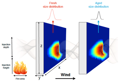
Figure 1Schematic of the 2D Lagrangian wall configuration of SAM-TOMAS and SAM-ASP v1.0. Reproduced from Sakamoto et al. (2016).
In this project, SAM was configured as a moving, 2D Lagrangian wall oriented normal to the mean wind direction in the layer of smoke injection (between 1200 and 1360 m in our example case shown here) as in Fig. 1, reproduced from Sakamoto et al. (2016). Note that wind shear in the meteorological dataset used for boundary conditions also impacts the coupled model – the downwind (x) direction is determined once and from then on the dynamics occur in this 2D plane based on the boundary condition forcing and the model advection and turbulence schemes. Stevens and Pierce (2014) showed that this 2D model configuration does well in simulating SO2 and NOx dispersion in power-plant plumes as compared to airborne measurements.
Photolysis rates are calculated in ASP using offline lookup tables generated by the Tropospheric Ultraviolet and Visible (TUV) radiation model (Bais et al., 2003) that depend on solar zenith angle and overhead O3 columns. SAM-ASP v1.0 does not currently account for the impact of aerosols on these photolysis rates. ASP is run as a subroutine in each SAM master time step (10 s for the simulations here). The SAM model handles all tracer transport and supplies the temperature, pressure, air density, solar zenith angle, mass emissions flux, and initial gas concentrations to ASP, while ASP calculates the gas and aerosol processes within each grid box. SAM-ASP v1.0 currently does not calculate deposition but may be added in the future (the plume does not contact the ground for the case described in this paper). The grid boxes in the 2D moving wall have a 500 m×500 m horizontal resolution with a 120 km total domain width (and 500 m in the with-wind direction, one box) and 40 m vertical resolution with a total vertical extent of 3 km. The simulation here was spun up for 1800 s prior to emissions following Stevens and Pierce (2014). The resolution and time steps described here are flexible and should be customized depending on plume and meteorological characteristics.
When ASP v2.1 is run as a Lagrangian box model, it needs the initial concentrations within the plume to be specified. However, as SAM-ASP v1.0 can simulate the dispersion of the smoke horizontally and vertically, we added the capability to calculate the initial concentrations based on the mass emissions flux (M, kg burned ), emission factors (EFs, g (kg burned)−1), and fire area (A, m2 and assumes a square shape) for biomass burning species (Akagi et al., 2011; Sakamoto et al., 2015). The formula is
where Δmq is the mass mixing ratio (kg q∕kg air) of species q, which are the units used in SAM for tracer species, and BM is the mass of air in the emission box (in kg). This allows SAM-ASP v1.0 to better represent a wide range of fire sizes and intensities. To reduce computation time, ASP is only called in the boxes that are impacted by smoke in each SAM time step, defined as any grid box having a concentration of CO greater than a user-defined threshold (based on background concentrations determined by ambient fire measurements, here 150 ppb). The coupled SAM-ASP v1.0 model was run on 12 processors with 4 GB each, which should be considered the minimum system requirements.
We evaluated the performance of the newly coupled SAM-ASP v1.0 model by comparing model output to observations of the Williams fire made by Akagi et al. (2012), which was previously simulated using ASP in a Lagrangian box model by Alvarado et al. (2015). Emission ratios for this simulation were based on observed relative background-corrected concentration close to the source from Alvarado et al. (2015) and included observed values for many gas-phase species measured by Akagi et al. (2012). Plume injection height was set to between 1200 and 1400 m, as this was the height at which the plume was observed to level off, where a small amount of vertical mixing can be seen as the plume ages.
The large-scale meteorological forcing in SAM-ASP v1.0 is driven by the 3 h, 32 km resolution North American Regional 30 Reanalysis (NARR; Messinger et al., 2006) meteorology dataset. The fire simulated in this study to evaluate the SAM-ASP v1.0 model was a prescribed fire measured on 17 November 2009 called the Williams fire (Akagi et al., 2012). This fire covered 81 ha north of Buellton, CA, with the fuel type classified as chaparral and the vegetation burned consisting of coastal sage scrub and scrub oak woodland understory. Surface temperatures ranged from 19 ∘C at 09:00 local time to 24 ∘C at 12:20 local time with clear skies throughout the fire duration. The plume built up gradually during the day with most of the smoke rising to ∼1200–1336 m above mean sea level and then drifting in a northeast direction. Two flights were conducted during the day on board a US Forest Services Twin Otter aircraft to sample initial emissions and aged smoke with an airborne Fourier transform infrared spectrometer instrument from the University of Montana taken during both flights including background measurements sampled at similar altitudes to in-plume measurements just outside the plume. Trace gas species emission factors determined as initial emissions (within minutes of the emission source) by Akagi et al. (2012) are used to initialize ASP and included: O3, nitrous acid (HONO), ammonia (NH3), ammonium (NH4), nitric oxide (NO), NO2, NOx (as NO), OA, and peroxy acetyl nitrate (PAN). Additional emission factors not measured, but needed to initialize ASP, were included using emission factors from Table 2 of Akagi et al. (2011), with the full list of ASP species provided in the model code repository described in Sect. 6. Initial aerosol size distribution information is inferred from the smoke study of Grieshop et al. (2009a, b). Full details of the fire and measurements are also further described in Akagi et al. (2012). Model input background concentrations were assumed based on measurements taken outside of the defined plume. Additional static inputs required by ASP include a photolysis rate parameterization based on the time and latitude of the fire and chemical data on aqueous phase ions and inorganics. Details of the static ASP inputs are further described in Alvarado (2008).
The model used here has 10 size bins with the total number of fire-emitted particles derived from multiplying the CO flux (based on measured values) by the ratio of particle number enhancement (number of particles cm−3) to CO enhancement (ppb) ( particles ). We use a number mean diameter of 0.1 µm and a standard deviation of 1.9 based on the wood smoke study of Grieshop et al. (2009a, b).
The NEMR calculations were determined by calculating the average species of interest (X) and CO concentration across the plume, as was done in the measurements. The NEMR (ΔX∕ΔCO or ΔX∕ΔCO2) is then calculated relative to CO or CO2 since they have relatively long lifetimes for the fire location, low background variability, and there were no other major nearby sources as described in Akagi et al. (2012):
Note that, in general, NEMRs are imprecise indicators of chemical changes, especially for plumes that have traveled far from their original source and may have mixed with different types of background air; thus, defining a single background concentration to subtract from the plume concentration is not a realistic approach (e.g., Yokelson et al., 2013). However, for the Williams fire, the excess mixing ratios downwind tended to vary slowly in time and space compared to measurement frequency, and the background value was computed from the average of a large number of points at the plume altitude (but outside the plume; Akagi et al., 2012).
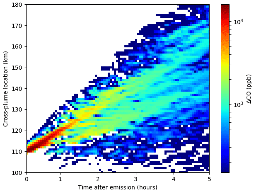
Figure 2SAM-ASP Williams fire simulation of cross-plume location versus time since emission at a vertical height of 1200 m for ΔCO. Note that figure is zoomed in on the plume with white background indicating a concentration of less than 150 ppb.
Averaged NEMR values over the full horizontal domain of the model for the vertical level with the peak ΔCO (and ΔCO2) can be used to compare with aircraft observations of biomass burning plumes. Figure 2 shows a horizontal slice of the simulated ΔCO concentrations (ppbv) as the plume moves downwind (bird's eye view at 1200 m above ground). Note that the initial plume was distributed across two horizontal gird boxes (initial plume width of 1 km) and four vertical grid boxes (initial height from 1200 to 1360 m) and was rectangular. The emissions were distributed proportional to the density of air in each grid box and initially propagated downward due to wind shear and diffusion. The dilution of the plume can be seen in the ΔCO values as high as 16 000 ppbv between the center of the plume within the first hour after initial emission to 5 h downwind, where the plume was modeled to be approximately 100 km wide, with an average in-plume ΔCO concentration of approximately 1000 ppbv. Figure 3 shows a vertical slice of (looking into) the plume at 1, 2, and 5 h downwind for ΔCO, ΔO3∕ΔCO, and ΔOA∕ΔCO2, and these results will be discussed in the following sections. Note that ΔCO2 was used to as the NEMR denominator for OA, as in Akagi et al. (2012) and Alvarado et al. (2015), as in the field study OA and CO2 were measured on the same inlet, while CO was measured on a different inlet. The uncertainty in the Lagrangian age (horizontal error bars in Fig. 3) was calculated as in Akagi et al. (2012), where the 1σ uncertainty in the average horizontal wind speeds during the sampling period were propagated through the plume age calculation, assuming the distance calculation was accurate.

Figure 3Height vs. cross-plume location at 1 h (left column), 2 h (center column) and 5 h (right column) downwind of fire source for ΔCO (top row), ΔO3∕ΔCO (ppb/ppb, center row), and ΔOA∕ΔCO2 (bottom row). Note that figure is zoomed in on the plume, and white indicates a CO concentration of less than 150 ppb.
For better comparison between the ASP v2.1 box model of Alvarado et al. (2015) and SAM-ASP v1.0, all emission ratios and background concentrations were made identical in box models. The same gas-phase chemical mechanism, aerosol thermodynamics routines and parameters, aerosol size distribution routines and parameters, and other chemical parameters were used. Thus the key difference between the two models is the treatment of plume dilution and mixing (with minor differences due to vertical temperature, pressure, and humidity variations in SAM-ASP v1.0 versus constant parameters used in ASP v2.1). In ASP v2.1, the plume is a single well-mixed box and dilution is parameterized by assuming a one-way addition of background air to the plume. As in Mason et al. (2001) we assume a Lagrangian parcel of fixed height (H) and length but variable width y(t). This assumes the plume is well-mixed vertically and capped at the top and bottom by a strong stable layer (or the surface). The temperature and pressure of the parcel are assumed to be constant. The effect of plume dispersion on concentrations is then (Mason et al., 2001; Alvarado, 2008)
where Cq is the concentration of species q within the parcel (molecules cm−3) and is the concentration of species q in the atmosphere outside of the parcel. The form of y(t) is assumed to be , where yo is the initial plume width (Mason et al., 2001). Ky represents the horizontal diffusivity of the atmosphere. The effect of plume dispersion then becomes
This equation is used with the observations of the rate of change in excess CO in the Williams fire plume to derive best fit values for Kyusing the observed value of yo.
In SAM-ASP v1.0, horizontal and vertical mixing between the boxes of the Lagrangian wall are calculated as part of the tracer transport routines of SAM 6.10.10 described in Sect. 2.2 (Khairoutdinov and Randall, 2003). In addition, unlike the ASP v2.1 box model of Alvarado et al. (2015), plume gradients are preserved in SAM-ASP v1.0. Thus, the chemistry taking place in the center of the plume may differ from that in the edges of the plume, potentially changing the plume-average NEMRs from those calculated with the well-mixed box assumption in ASP v2.1.
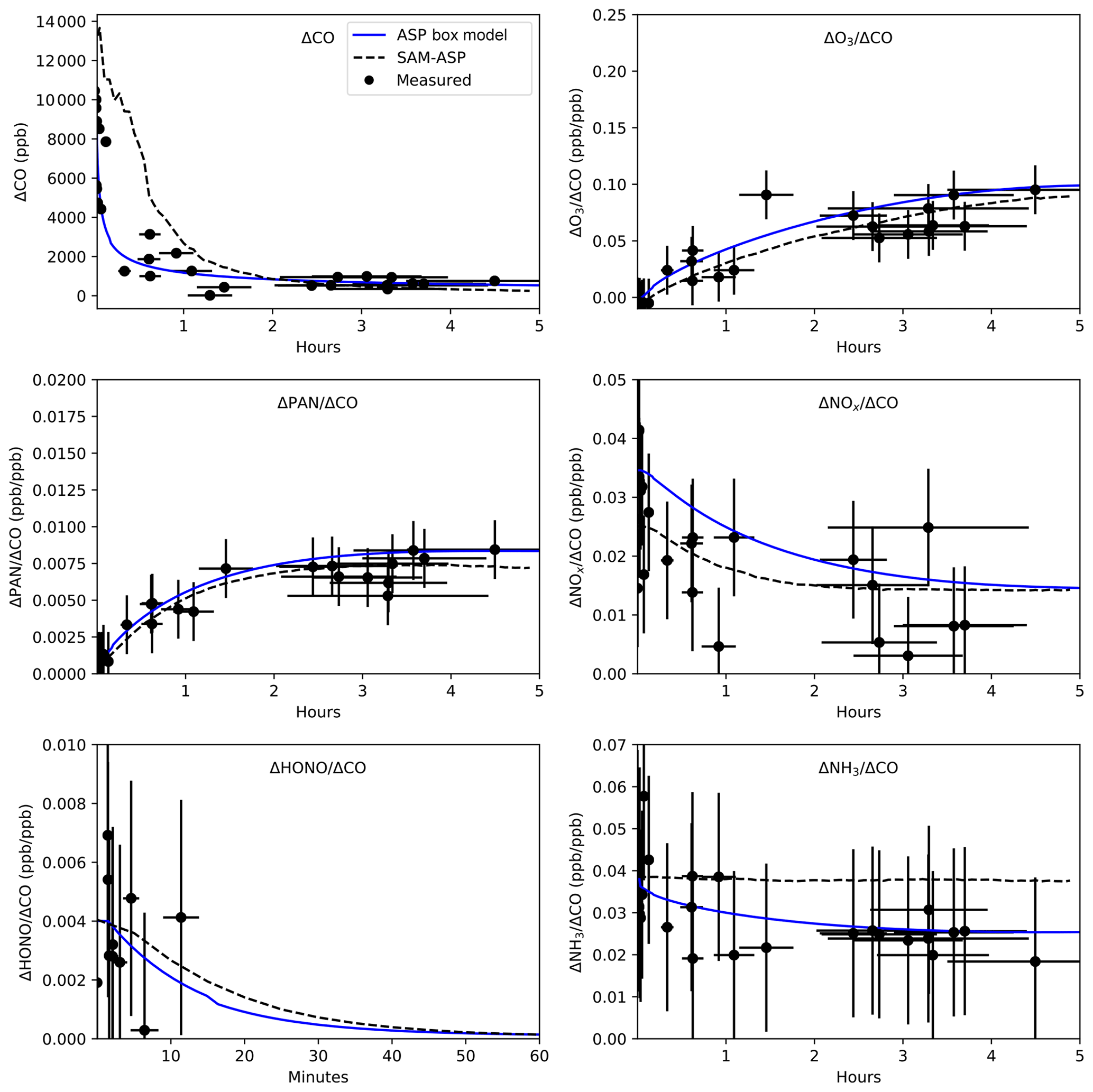
Figure 4Cross-plume-averaged ΔCO and O3, PAN, NOx, HONO, and NH3 NEMRs (ΔX∕ΔCO) as a function of plume age for the ASP box model (solid line, reproduced from Alvarado et al., 2015) and SAM-ASP model (dashed line) results compared to measurements from Akagi et al. (2012) (dots). The horizontal error bars indicate the age uncertainty of the measurements, while the vertical errors bars are the uncertainty of the measured value.
3.1 Gas-phase simulations
The in-plume CO enhancement ( CObackground, in ppbv) and NEMRs (Eq. 1) for O3, are shown in Figs. 3 and 4. NEMRs for PAN, NOx, HONO and NH3 are shown in just Fig. 4, where the average NEMR across SAM-ASP v1.0 grid boxes is calculated where the CO concentrations are above a background threshold of 150 ppbv (based on measurements). In Fig. 4, horizontal error bars indicate the age uncertainty of the measurements, with a best estimate of the starting NEMR and uncertainty discussed in Akagi et al. (2012), which uses a slope-based fire-average emission ratio (ER) as a best estimate of the likely starting NEMR for primary species measured in individual smoke transects. The SAM-ASP v1.0 model was qualitatively able to simulate the dilution of CO in the smoke plume after 2 h to within the uncertainties of the measurements but with an underestimate of dispersion in the first 2 h. As ASP v2.1 currently uses a fixed function to simulate dilution, we were unable to test how using the SAM-ASP predicted dilution of CO to ASP v2.1 would alter the box model results. SAM-ASP v1.0 also correctly simulated the chemical loss of NOx and HONO and the formation of PAN and O3 within the plume. After 2 h of model-simulated O3 (second row in Fig. 3), it can be seen that the edges of the plume have higher concentrations than the center, a feature that cannot be represented in a box model simulation. This O3 enhancement at the edges may be a result of less NO titration at the plume edges. We expect larger O3 edge effects in future work when the TUV radiation model is coupled online and interacts with plume aerosols. NH3 concentrations in the model were overestimated (model value of ΔNH3∕ΔCO of 0.04 ppb ppb−1 at 5 h, rather than the measured value of 0.02 mol mol−1). This is in contrast to the results of the ASP Lagrangian box model study of Alvarado et al. (2015), where the box model-simulated NH3 closer to measured values at all hours downwind. The results for this gas are very sensitive to the amount of sulfate and nitrate formed in the plume, the dilution of the plume as it affects the volatilization of NH3 from the aerosol, as well as the relative humidity and temperature, all of which differ slightly between ASP v2.1 and SAM-ASP v1.0, but we have not yet determined which difference is driving the ammonia discrepancy. The lack of vertical variation in the SAM-ASP plume in Fig. 3 may be due to the use of photolysis rates that are not altered by the simulated aerosol scattering and absorption in this version of SAM-ASP. Thus, while the photolysis rates vary with time, they do not vary horizontally or vertically, with future work needed to incorporate in-line, vertically varying photolysis consideration.
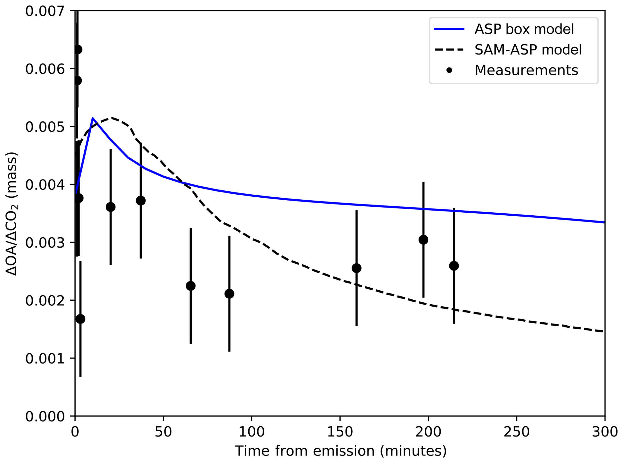
Figure 5Cross-plume-averaged OA NEMR (ΔOA∕ΔCO2) for the Williams fire from SAM-ASP simulations (dashed line), the ASP box model results as described in Alvarado et al. (2015) (solid lines), and OA measurements (back dots) described in Akagi et al. (2012).
3.2 Aerosol simulations
OA NEMR results from the ASP box model (Alvarado et al., 2015) and measurements from Akagi et al. (2012) are compared to cross-plume-averaged SAM-ASP output in Fig. 5. In general, the SAM-ASP results show slightly slower initial dilution than the box model, with the initial increase in OA due to the 2D wall staying over the emission area; thus evaporatively driven decreases have not dominated yet. This difference in dilution rate, and thus OA NEMR, is due to dilution in the box being forced to match measurements while in SAM-ASP, the meteorology, and initial plume width determine the relative dispersion rate (Alvarado et al., 2015). Within the first hour after emission, SAM-ASP has less dilution than the box model (Figs. 4a and 5), leading to a higher OA concentration, which in turn leads to less evaporation of OA to intermediate and semi-volatile vapors, explaining the larger OA NEMR for this initial time period. However, SAM-ASP has greater dilution than the box model after 2 h (though both falling within measurement uncertainties in Fig. 4a), which leads to more OA evaporation in SAM-ASP than in the box model, leading to a lower OA NEMR after 2 h, better matching the measurements. We note, however, that there are considerable uncertainties in the volatility distribution of the simulated POA as well as the SOA chemistry, so there may be multiple ways to improve modeled OA NEMR. The bottom panels of Fig. 3 show that the OA NEMR in the model initially decreases faster than the core, driven by dilution. However, after several hours the OA NEMR at the edges increases, showing that SOA production in those locations is exceeding evaporation in those locations. Thus, in both models the initial POA partially evaporates, but this is balanced by oxidation of the S/IVOCs in the gas phase, which then condense as SOA. This initial evaporation followed by net SOA production is consistent with the theoretical studies of Bian et al. (2017) and Hodshire et al. (2019b); however, those studies did not explore this behavior in the plume edges versus the core. SAM-ASP will be used in future work to investigate these plume edge versus core differences within field observations.
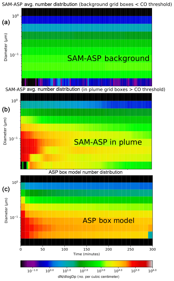
Figure 6SAM-ASP (a, b) and ASP box model (c) simulated particle size distribution (dN∕dlog Dp cm−3) evolution within the Williams fire.
We also compared the predictions for aerosol size distribution changes between the two models (Fig. 6). Note that as no size distribution measurements were taken for this fire, we cannot compare these simulations with observations. Figure 6a shows the average size distribution of the background air in the SAM-ASP simulation. We again average the SAM-ASP results across grid boxes where CO concentration are above the CO threshold (150 ppbv) in each time step. Both models suggest that this fire showed little net aerosol diameter growth (Fig. 6b, c), as shrinking due to evaporative losses driven by dilution compensates for growth by coagulation and the oxidation (and reduction in volatility) of the organic vapors, consistent with the OA NEMR results above.
We have described a new coupled model, SAM-ASP v1.0, for simulating the gas and aerosol chemistry within biomass burning smoke plumes. The model adds the Aerosol Simulation Program v2.1 (ASP v2.1) as an embedded subroutine within the System for Atmospheric Modeling v6.10 (SAM v6.10). When configured as a 2D Lagrangian wall, the newly coupled SAM-ASP model allows for a detailed examination of the chemical and physical evolution of fine-scale biomass burning plumes.
SAM-ASP is able to simulate the complex, non-linear production of O3 and changes in PM as plumes age. It is able to resolve the cross-plume chemistry, gas-to-particle partitioning, and microphysics that coarser grid-scale CTMs are not able to. Model results indicate that SAM-ASP is able to accurately simulate the dilution of CO in a California chaparral smoke plume mostly, except for a slight initial underprediction, as well as accurately predict the chemical loss of NOx and HONO and the production of O3 and PAN within the plume. SAM-ASP also resolves the cross-plume concentration of trace gases and aerosol. However, when compared to observations, the simulation with SAM-ASP did not show any significant differences with respect to a much simpler box model simulation, potentially because the photolysis rates within both simulations were identical rather than allowing the photolysis rates to vary with predicted aerosol concentrations.
Future work will involve testing SAM-ASP simulations against observed plume crosswind and vertical gradients as well as size distributions. Future work will also include the development of a biomass burning parameterization of plume-scale chemical and physical trace gas and aerosol evolution for use in coarser grid-scale CTMs (that cannot resolve plumes) as well as the implementation of on-line photolysis calculations to explicitly simulate the effect of in-plume aerosols on photolysis rates.
SAM-ASP 1.0 source code is available for download through the SAM website at http://rossby.msrc.sunysb.edu/~marat/SAM.html (last access: 23 September 2020) through request to the SAM model developer, Marat Khairoutdinov. Separate ASP model code, model inputs, outputs, and 15 post-processing steps described in this study are available in a public repository at https://doi.org/10.5281/zenodo.3363995 (Lonsdale, 2019).
CRL provided the design and performed the execution of the model implementation, simulation, and evaluation of the SAM-ASP code and prepared this paper. MJA and JRP provided oversight and leadership of the overall development and acquired the financial support for the project leading to this publication, as well as contributing to the review and editing of this paper. ALH and ER provided verification of the overall reproducibility of model results, presented complementary published work, and contributed to the review and editing of this paper.
The authors declare that they have no conflict of interest.
This work was supported by NOAA Atmospheric Chemistry, Carbon Cycle and Climate Program award nos. NA17OAR4310001, NA17OAR4310002, and NA17OAR4310009, as well as NSF Atmospheric Chemistry Program grant nos. 1559598 and 1559607 as well as by the State of Texas through the Air Quality Research Program administered by The University of Texas at Austin by means of a grant from the Texas Commission on Environmental Quality.
This research has been supported by the AQRP through a grant from the Texas Commission on Environmental Quality (grant no. AQRP 16-024), the NOAA Atmospheric Chemistry, Carbon Cycle and Climate Program (grant nos. NA17OAR430001, NA17OAR4310002, and NA17OAR4310009), and the NSF Atmospheric Chemistry Program Grants (grant nos. 1559598 and 1559607).
This paper was edited by Christoph Knote and reviewed by two anonymous referees.
Ahmadov, R., McKeen, S. A., Robinson, A. L., Bahreini, R., Middlebrook, A. M., de Gouw, J. A., Meagher, J., Hsie, E.-Y., Edgerton, E., Shaw, S., and Trainer, M.: A volatility basis set model for summertime secondary organic aerosols over the eastern United States in 2006, J. Geophys. Res., 117, 2156–2202, 2012.
Akagi, S. K., Yokelson, R. J., Wiedinmyer, C., Alvarado, M. J., Reid, J. S., Karl, T., Crounse, J. D., and Wennberg, P. O.: Emission factors for open and domestic biomass burning for use in atmospheric models, Atmos. Chem. Phys., 11, 4039–4072, https://doi.org/10.5194/acp-11-4039-2011, 2011.
Akagi, S. K., Craven, J. S., Taylor, J. W., McMeeking, G. R., Yokelson, R. J., Burling, I. R., Urbanski, S. P., Wold, C. E., Seinfeld, J. H., Coe, H., Alvarado, M. J., and Weise, D. R.: Evolution of trace gases and particles emitted by a chaparral fire in California, Atmos. Chem. Phys., 12, 1397–1421, https://doi.org/10.5194/acp-12-1397-2012, 2012.
Alvarado, M. J.: Formation of ozone and growth of aerosols in young smoke plumes from biomass burning, PhD thesis, Massachusetts Institute of Technology, Cambridge, MA, USA, 324 pp., available at: https://globalchange.mit.edu/publication/13991 (last access: 23 September 2020), 2008.
Alvarado, M. J. and Prinn, R. G.: Formation of ozone and growth of aerosols in young smoke plumes from biomass burning, Part 1: Lagrangian parcel studies, J. Geophys. Res., 114, D09306, https://doi.org/10.1029/2008JD011144, 2009.
Alvarado, M. J., Wang, C., and Prinn, R. G.: Formation of ozone and growth of aerosols in young smoke plumes from biomass burning, Part 2: 3D Eulerian studies, J. Geophys. Res., 114, D09307, https://doi.org/10.1029/2008JD011186, 2009.
Alvarado, M. J., Logan, J. A., Mao, J., Apel, E., Riemer, D., Blake, D., Cohen, R. C., Min, K.-E., Perring, A. E., Browne, E. C., Wooldridge, P. J., Diskin, G. S., Sachse, G. W., Fuelberg, H., Sessions, W. R., Harrigan, D. L., Huey, G., Liao, J., Case-Hanks, A., Jimenez, J. L., Cubison, M. J., Vay, S. A., Weinheimer, A. J., Knapp, D. J., Montzka, D. D., Flocke, F. M., Pollack, I. B., Wennberg, P. O., Kurten, A., Crounse, J., Clair, J. M. St., Wisthaler, A., Mikoviny, T., Yantosca, R. M., Carouge, C. C., and Le Sager, P.: Nitrogen oxides and PAN in plumes from boreal fires during ARCTAS-B and their impact on ozone: an integrated analysis of aircraft and satellite observations, Atmos. Chem. Phys., 10, 9739–9760, https://doi.org/10.5194/acp-10-9739-2010, 2010.
Alvarado, M. J., Lonsdale, C. R., Yokelson, R. J., Akagi, S. K., Coe, H., Craven, J. S., Fischer, E. V., McMeeking, G. R., Seinfeld, J. H., Soni, T., Taylor, J. W., Weise, D. R., and Wold, C. E.: Investigating the links between ozone and organic aerosol chemistry in a biomass burning plume from a prescribed fire in California chaparral, Atmos. Chem. Phys., 15, 6667–6688, https://doi.org/10.5194/acp-15-6667-2015, 2015.
Alvarado, M. J., Lonsdale, C. R., Macintyre, H. L., Bian, H., Chin, M., Ridley, D. A., Heald, C. L., Thornhill, K. L., Anderson, B. E., Cubison, M. J., Jimenez, J. L., Kondo, Y., Sahu, L. K., Dibb, J. E., and Wang, C.: Evaluating model parameterizations of submicron aerosol scattering and absorption with in situ data from ARCTAS 2008, Atmos. Chem. Phys., 16, 9435–9455, https://doi.org/10.5194/acp-16-9435-2016, 2016.
Bais, A. F., Madronich, S., Crawford, J., Hall, S. R., Mayer, B., van Weele, M., Lenoble, J., Calvert, J. G., Cantrell, C. A., Shetter, R. E., Hofzumahaus, A., Koepke, P., Monks, P. S., Frost, G., McKenzie, R., Krotkov, N., Kylling, A., Swartz, W. H., Lloyd, S., Pfister, G., Martin, T. J., Roeth, E., Griffioen, E., Ruggaber, A., Krol, M., Kraus, A., Edwards, G. D., Mueller, M., Lefer, B. L., Johnston, P., Schwander, H., Flittner, D., Gardiner, B. G., Barrick, J., and Schmitt, R.: International photolysis frequency measurement and model intercomparison: Spectral actinic solar flux measurements and modeling, J. Geophys. Res., 108, 8543, https://doi.org/10.1029/2002JD002891, 2003.
Baker, K.: Simulating fire event impacts on regional O3 and PM2.5 and looking toward evaluation, 14th Annual CMAS Conference, UNC-Chapel Hill, 5–7 October 2015.
Baylon, P., Jaffe, D., Hall, S., Ullmann, K., Alvarado, M., and Lefer, B.: Impact of Biomass Burning Plumes on Photolysis Rates and Ozone Formation at the Mount Bachelor Observatory, J. Geophys. Res.-Atmos., 123, 2272–2284, 2018.
Bian, Q., Jathar, S. H., Kodros, J. K., Barsanti, K. C., Hatch, L. E., May, A. A., Kreidenweis, S. M., and Pierce, J. R.: Secondary organic aerosol formation in biomass-burning plumes: theoretical analysis of lab studies and ambient plumes, Atmos. Chem. Phys., 17, 5459–5475, https://doi.org/10.5194/acp-17-5459-2017, 2017.
Bloss, C., Wagner, V., Jenkin, M. E., Volkamer, R., Bloss, W. J., Lee, J. D., Heard, D. E., Wirtz, K., Martin-Reviejo, M., Rea, G., Wenger, J. C., and Pilling, M. J.: Development of a detailed chemical mechanism (MCMv3.1) for the atmospheric oxidation of aromatic hydrocarbons, Atmos. Chem. Phys., 5, 641–664, https://doi.org/10.5194/acp-5-641-2005, 2005.
Bond, T. C., Doherty, S. J., Fahey, D. W., Forster, P. M., Berntsen, T., DeAngelo, B. J., Flanner, M. G., Ghan, S., Kärcher, B., Koch, D., Kinne, S., Kondo, Y., Quinn, P. K., Sarofim, M. C., Schultz, M. G., Schulz, M., Venkataraman, C., Zhang, H., Zhang, S., Bellouin, N., Guttikunda, S. K., Hopke, P. K., Jacobson, M. Z., Kaiser, J. W., Klimont, Z., Lohmann, U., Schwarz, J. P., Shindell, D., Storelvmo, T., Warren, S. G., and Zender, C. S.: Bounding the role of black carbon in the climate system: A scientific assessment, J. Geophys. Res.-Atmos., 118, 5380–5552, 2013.
Boucher, O., Randall, D., Artaxo, P., Bretherton, C., Feingold, G., Forster, P., Kerminen, V.-M., Kondo, Y., Liao, H., Lohmann, U., Rasch, P., Satheesh, S. K., Sherwood, S., Stevens, B., and Zhang, X. Y.: Climate Change 2013: The Physical Science Basis. Contribution of Working Group I to the Fifth Assessment Report of the Intergovernmental Panel on Climate Change, edited by: Stocker, T. F., Qin, D., Plattner, G.-K., Tignor, M., Allen, S. K., Boschung, J., Nauels, A., Xia, Y., Bex, V., and Midgley, P. M., Cambridge University Press, Cambridge, United Kingdom and New York, NY, USA, 2013.
Collier, S., Zhou, S., Onasch, T. B., Jaffe, D. A., Kleinman, L., Sedlacek, A. J. III, Briggs, N. L., Hee, J., Fortner, E., Shilling, J. E.,Worsnop, D., Yokelson, R. J., Parworth, C., Ge, X., Xu, J., Butterfield, Z., Chand, D., Dubey, M. K., Pekour, M. S., Springston, S., and Zhang, Q.: Regional influence of aerosol emissions from wildfires driven by combustion efficiency: Insights from the BBOP campaign, Environ. Sci. Tech., 50, 8613–8622, 2016.
Crounse, J. D., Paulot, F., Kjaergaard, H. G., and Wennberg, P. O.:Peroxy radical isomerization in the oxidation of isoprene, Phys. Chem. Chem. Phys., 13, 13607–13613, 2011.
Crounse, J. D., Knap, H. C., Ørnsø, K. B., Jørgensen, S., Paulot, F., Kjaergaard, H. G., and Wennberg, P. O.: Atmospheric fate of methacrolein. 1. Peroxy radical isomerization following addition of OH and O2, J. Phys. Chem. A, 116, 5756–5762, https://doi.org/10.1021/jp211560u, 2012.
Dzepina, K., Volkamer, R. M., Madronich, S., Tulet, P., Ulbrich, I. M., Zhang, Q., Cappa, C. D., Ziemann, P. J., and Jimenez, J. L.: Evaluation of recently-proposed secondary organic aerosol models for a case study in Mexico City, Atmos. Chem. Phys., 9, 5681–5709, https://doi.org/10.5194/acp-9-5681-2009, 2009.
European Environment Agency. Air quality in Europe – 2018 report, available at: https://www.eea.europa.eu/publications/air-quality-in-europe-2018/download (last access: 2 May 2019), 2018.
Fan, J., Ovtchinnikov, M., Comstock, J. M., McFarlane, S. A., and Khain, A.: Ice formation in Arctic mixed-phase clouds: Insights from a 3-D cloud-resolving model with size-resolved aerosol and cloud microphysics, J. Geophys. Res.-Atmos., 114, D04205, https://doi.org/10.1029/2008JD010782, 2009.
Flynn, J., Lefer, B., Rappenglück, B., Leuchner, M., Perna, R., Dibb, J., Ziemba, L., Anderson, C., Stutz, J., Brune, W., Ren, X., Mao, J., Luke, W., Olson, J., Chen, G., and Crawford, J.: Impact of clouds and aerosols on ozone production in Southeast Texas, Atmos. Environ., 44, 4126–4133, https://doi.org/10.1016/j.atmosenv.2009.09.005, 2010.
Garofalo, L. A., Pothier, M. A., Levin, E. J., Campos, T., Kreidenweis, S. M., and Farmer, D. K.: Emission and Evolution of Submicron Organic Aerosol in Smoke from Wildfires in the Western United States, ACS Earth and Space Chemistry, 3, 1237–1247, 2019.
Goliff, W. S., Stockwell, W. R., and Lawson, C. V.: The regional atmospheric chemistry mechanism, version 2, Atmos. Environ., 68, 174–185, 2013.
Goodrick, S. L., Achtemeier, G. L., Larkin, N. K., Liu, Y., and Strand, T. M.: Modelling smoke transport from wildland fires: a review, Int. J. Wildland Fire, 22, 83–94, 2013.
Grieshop, A. P., Logue, J. M., Donahue, N. M., and Robinson, A. L.: Laboratory investigation of photochemical oxidation of organic aerosol from wood fires 1: measurement and simulation of organic aerosol evolution, Atmos. Chem. Phys., 9, 1263–1277, https://doi.org/10.5194/acp-9-1263-2009, 2009a.
Grieshop, A. P., Donahue, N. M., and Robinson, A. L.: Laboratory investigation of photochemical oxidation of organic aerosol from wood fires 2: analysis of aerosol mass spectrometer data, Atmos. Chem. Phys., 9, 2227–2240, https://doi.org/10.5194/acp-9-2227-2009, 2009b.
Hess, M., Koepke, P., and Schult, I.: Optical Properties of Aerosols and clouds: The software package OPAC, B. Am. Meteorol. Soc., 79, 831–844, 1998.
Hobbs, P. V., Sinha, P., Yokelson, R. J., Christian, T. J., Blake, D. R., Gao, S., Kirschstetter, T. W., Novakov, T., and Pilewskie, P.: Evolution of gases and particles from a savanna fire in South Africa, J. Geophys. Res., 108, 8485, https://doi.org/10.1029/2002JD002352, 2003.
Hodshire, A. L., Akherati, A., Alvarado, M. J., Brown-Steiner, B., Jathar, S. H., Jimenez, J. L., Kreidenweis, S. M., Lonsdale, C. R., Onasch, T. B., Ortega, A. M., and Pierce, J. R.: Aging Effects on Biomass Burning Aerosol Mass and Composition: A Critical Review of Field and Laboratory Studies, Env. Sci. Tech., 53, 10007–10022, https://doi.org/10.1021/acs.est.9b02588, 2019a.
Hodshire, A. L., Bian, Q., Ramnarine, E., Lonsdale, C. R., Alvarado, M. J., Kreidenweis, S. M., Jathar, S. H., and Pierce, J. R.: More than emissions and chemistry: Fire size, dilution, and background aerosol also greatly influence near-field biomass burning aerosol aging, J. Geophys. Res., 124, 5589–5611, https://doi.org/10.1029/2018JD029674, 2019b.
Hosseini, S., Li, Q., Cocker, D., Weise, D., Miller, A., Shrivastava, M., Miller, J. W., Mahalingam, S., Princevac, M., and Jung, H.: Particle size distributions from laboratory-scale biomass fires using fast response instruments, Atmos. Chem. Phys., 10, 8065–8076, https://doi.org/10.5194/acp-10-8065-2010, 2010.
Jacobson, M. Z.: Analysis of aerosol interactions with numerical techniques for solving coagulation, nucleation, condensation, dissolution, and reversible chemistry among multiple size distributions, J. Geophys. Res., 107, 4366, https://doi.org/10.1029/2001JD002044, 2002.
Jacobson, M. Z.: Fundamentals of Atmospheric Modelling, 2nd ed., Cambridge University Press, Cambridge, UK, 2005.
Janhäll, S., Andreae, M. O., and Pöschl, U.: Biomass burning aerosol emissions from vegetation fires: particle number and mass emission factors and size distributions, Atmos. Chem. Phys., 10, 1427–1439, https://doi.org/10.5194/acp-10-1427-2010, 2010.
Jenkin, M. E., Saunders, S. M., and Pilling, M. J.: The tropospheric degradation of volatile organic compounds: A protocol for mechanism development, Atmos. Environ., 31, 81–104, 1997.
Jenkin, M. E., Saunders, S. M., Wagner, V., and Pilling, M. J.: Protocol for the development of the Master Chemical Mechanism, MCM v3 (Part B): tropospheric degradation of aromatic volatile organic compounds, Atmos. Chem. Phys., 3, 181–193, https://doi.org/10.5194/acp-3-181-2003, 2003.
Khairoutdinov, M. F. and Kogan, Y. L.: A large eddy simulation model with explicit microphysics: Validation against aircraft observations of a stratocumulus-topped boundary layer, J. Atmos. Sci., 56, 2115–2131, 1999.
Khairoutdinov, M. F. and Randall, D. A.: Cloud resolving modeling of the ARM summer 1997 IOP: Model formulation, results, uncertainties, and sensitivities, J. Atmos. Sci., 60, 607–625, 2003.
Knorr, W., Dentener, F., Lamarque, J.-F., Jiang, L., and Arneth, A.: Wildfire air pollution hazard during the 21st century, Atmos. Chem. Phys., 17, 9223–9236, https://doi.org/10.5194/acp-17-9223-2017, 2017.
Konovalov, I. B., Beekmann, M., Golovushkin, N. A., and Andreae, M. O.: Nonlinear behavior of organic aerosol in biomass burning plumes: a microphysical model analysis, Atmos. Chem. Phys., 19, 12091–12119, https://doi.org/10.5194/acp-19-12091-2019, 2019.
Lee, L. A., Pringle, K. J., Reddington, C. L., Mann, G. W., Stier, P., Spracklen, D. V., Pierce, J. R., and Carslaw, K. S.: The magnitude and causes of uncertainty in global model simulations of cloud condensation nuclei, Atmos. Chem. Phys., 13, 8879–8914, https://doi.org/10.5194/acp-13-8879-2013, 2013.
Lonsdale, C.: Simulating Forest Fire Plume Dispersion, Chemistry, and Aerosol Formation Using SAM-ASP version 1.0, Zenodo, https://doi.org/10.5281/zenodo.3363995, 2019.
Lonsdale, C. R., Stevens, R. G., Brock, C. A., Makar, P. A., Knipping, E. M., and Pierce, J. R.: The effect of coal-fired power-plant SO2 and NOx control technologies on aerosol nucleation in the source plumes, Atmos. Chem. Phys., 12, 11519–11531, https://doi.org/10.5194/acp-12-11519-2012, 2012.
Lonsdale, C. R., Alvarado, M. J., Yokelson, R. J., Akagi, S. K., Fischer, E., Travis, K., Soni, T., Craven, J. S., Taylor, J. W., McMeeking, G. R., Burling, I. R., Urbanski, S. P., Wold, C. E., Seinfeld, J. H., Coe, H., and Weise, D. R.: Modeling the Chemistry and Growth of Organic Aerosol in Biomass Burning Plumes at Local and Regional Scales, American Association for Aerosol Research, Minneapolis, MN, 12–16 October 2015.
Magi, B. I. and Hobbs, P. V.: Effects of humidity on aerosols in southern Africa during the biomass burning season, J. Geophys. Res., 108, 8495, https://doi.org/10.1029/2002JD002144, 2003.
Mason, S. A., Field, R. J., Yokelson, R. J., Kochivar, M. A., Tinsley, M. R., Ward, D. E., and Hao, W. M.: Complex effects arising in smoke plume simulations due to the inclusion of direct emissions of oxygenated organic species from biomass combustion, J. Geophys. Res., 106, 12527–12539, 2001.
Maxwell Garnet, J. C.: Colours in metal glasses and in metallic films, Philos. T. R. Soc. A, 203, 385–420, 1904.
McClure, C. D. and Jaffe, D. A.: U.S. particulate matter air quality improves except in wildfire-prone areas, P. Natl. Acad. Sci. USA, 115, 7901–7906, https://doi.org/10.1073/pnas.1804353115, 2018.
McDonald-Buller, E., Kimura, Y., Wiedinmyer, C., Emery, C., Liu, Z., and Yarwood, G.: Targeted Improvements in the Fire Inventory form NCAR (FINN) Model for Texas Air Quality Planning, Final Report to Texas Air Quality Research Program (AQRP) for Project 14-011, December 2015.
Messinger, F., DiMego, G., Kalnay, E., Mitchell, K., Shafran, P. C., Ebisuzaki, W., Jović, D., Woollen, J., Rogers, E., Berbery, E. H., and Ek, M. B.: North American regional reanalysis, B. Am. Meteorol. Soc., 87, 343–360, 2006.
Morrison, H. C. J. A., Curry, J. A., and Khvorostyanov, V. I.: A new double-moment microphysics parameterization for application in cloud and climate models. Part I: Description, J. Atmos. Sci., 62, 1665–1677, 2005.
O'Dell, K., Ford, B., Fischer, E., and Pierce, J.: The contribution of wildland-fire smoke to US PM2.5 and its influence on recent trends, Environ. Sci. Technol., 53, 1797–1804, https://doi.org/10.1021/acs.est.8b05430, 2019.
Ordóñez, C., Elguindi, N., Stein, O., Huijnen, V., Flemming, J., Inness, A., Flentje, H., Katragkou, E., Moinat, P., Peuch, V.-H., Segers, A., Thouret, V., Athier, G., van Weele, M., Zerefos, C. S., Cammas, J.-P., and Schultz, M. G.: Global model simulations of air pollution during the 2003 European heat wave, Atmos. Chem. Phys., 10, 789–815, https://doi.org/10.5194/acp-10-789-2010, 2010.
Ovchinnikov, M., Ackerman, A. S., Avramov, A., Cheng, A., Fan, J., Fridlind, A. M., Ghan, S., Harrington, J., Hoose, C., Korolev, A., McFarquhar, G. M., Morrison, H., Paukert, M., Savre, J., Shipway, B. J., Shupe, M. D., Solomon, A., and Sulia, K.: Intercomparison of large-eddy simulations of Arctic mixed-phase clouds: Importance of ice size distribution assumptions, J. Adv. Model. Earth Sys., 6, 223–248, 2014.
Paulot, F., Crounse, J. D., Kjaergaard, H. G., Kroll, J. H., Seinfeld, J. H., and Wennberg, P. O.: Isoprene photooxidation: new insights into the production of acids and organic nitrates, Atmos. Chem. Phys., 9, 1479–1501, https://doi.org/10.5194/acp-9-1479-2009, 2009a.
Paulot, F., Crounse, J. D., Kjaergaard, H. G., Kurten, A., St. Clair, J. M., Seinfeld, J. H., and Wennberg, P. O.: Unexpected epoxide formation in the gas-phase photooxidation of isoprene, Science, 325, 730–733, https://doi.org/10.1126/science.1172910, 2009b.
Petters, M. D. and Kreidenweis, S. M.: A single parameter representation of hygroscopic growth and cloud condensation nucleus activity, Atmos. Chem. Phys., 7, 1961–1971, https://doi.org/10.5194/acp-7-1961-2007, 2007.
Pierce, J. R., Chen, K., and Adams, P. J.: Contribution of primary carbonaceous aerosol to cloud condensation nuclei: processes and uncertainties evaluated with a global aerosol microphysics model, Atmos. Chem. Phys., 7, 5447–5466, https://doi.org/10.5194/acp-7-5447-2007, 2007.
Ramnarine, E., Kodros, J. K., Hodshire, A. L., Lonsdale, C. R., Alvarado, M. J., and Pierce, J. R.: Effects of near-source coagulation of biomass burning aerosols on global predictions of aerosol size distributions and implications for aerosol radiative effects, Atmos. Chem. Phys., 19, 6561–6577, https://doi.org/10.5194/acp-19-6561-2019, 2019.
Reid, J. S., Koppmann, R., Eck, T. F., and Eleuterio, D. P.: A review of biomass burning emissions part II: intensive physical properties of biomass burning particles, Atmos. Chem. Phys., 5, 799–825, https://doi.org/10.5194/acp-5-799-2005, 2005.
Robinson, A. L., Donahue, N. M., Shrivastava, M. K., Weitkamp, E. A., Sage, A. M., Grieshop, A. P., Lane, T. E., Pierce, J. R., and Pandis, S. N.: Rethinking organic aerosols: semivolatile emissions and photochemical aging, Science, 315, 1259–1262, 2007.
Sakamoto, K. M., Allan, J. D., Coe, H., Taylor, J. W., Duck, T. J., and Pierce, J. R.: Aged boreal biomass-burning aerosol size distributions from BORTAS 2011, Atmos. Chem. Phys., 15, 1633–1646, https://doi.org/10.5194/acp-15-1633-2015, 2015.
Sakamoto, K. M., Laing, J. R., Stevens, R. G., Jaffe, D. A., and Pierce, J. R.: The evolution of biomass-burning aerosol size distributions due to coagulation: dependence on fire and meteorological details and parameterization, Atmos. Chem. Phys., 16, 7709–7724, https://doi.org/10.5194/acp-16-7709-2016, 2016.
Saunders, S. M., Jenkin, M. E., Derwent, R. G., and Pilling, M. J.: Protocol for the development of the Master Chemical Mechanism, MCM v3 (Part A): tropospheric degradation of non-aromatic volatile organic compounds, Atmos. Chem. Phys., 3, 161–180, https://doi.org/10.5194/acp-3-161-2003, 2003.
Seinfeld, J. H. and Pandis, S. N.: Atmospheric Chemistry and Physics: From Air Pollution to Climate Change, John Wiley & Sons, Hoboken, 2016.
Shrivastava, M. K. B., Zelenyuk, A., Imre, D., Easter Jr., R. C., Beranek, J., Zaveri, R. A., and Fast, J. D.: Implications of Low Volatility SOA and Gas-Phase Fragmentation Reactions on SOA Loadings and their Spatial and Temporal Evolution in the Atmosphere, J. Geophys. Res., 118, 3328–3342, https://doi.org/10.1002/jgrd.50160, 2013.
Smolarkiewicz, P. K. and Grabowski, W. W.: The multidimensional positive definite advection transport algorithm: Nonoscillatory option, J. Comput. Phys., 86, 355–375, 1990.
Spracklen, D. V., Carslaw, K. S., Pöschl, U., Rap, A., and Forster, P. M.: Global cloud condensation nuclei influenced by carbonaceous combustion aerosol, Atmos. Chem. Phys., 11, 9067–9087, https://doi.org/10.5194/acp-11-9067-2011, 2011.
Stevens, R. G. and Pierce, J. R.: The contribution of plume-scale nucleation to global and regional aerosol and CCN concentrations: evaluation and sensitivity to emissions changes, Atmos. Chem. Phys., 14, 13661–13679, https://doi.org/10.5194/acp-14-13661-2014, 2014.
Stevens, R. G., Pierce, J. R., Brock, C. A., Reed, M. K., Crawford, J. H., Holloway, J. S., Ryerson, T. B., Huey, L. G., and Nowak, J. B.: Nucleation and growth of sulfate aerosol in coal-fired power plant plumes: sensitivity to background aerosol and meteorology, Atmos. Chem. Phys., 12, 189–206, https://doi.org/10.5194/acp-12-189-2012, 2012.
Tang, I. N.: Thermodynamic and optical properties of mixed-salt aerosols of atmospheric importance, J. Geophys. Res., 102, 1883, https://doi.org/10.1029/96JD03085, 1997.
Toon, O. B. and Ackerman, T. P.: Algorithms for the calculation of scattering by stratied spheres, Appl. Optics, 20, 3657–3660, https://doi.org/10.1364/AO.20.003657, 1981.
Trentmann, J., Fruh, B., Boucher, O., Trautmann, T., and Andreae, M. O.: Three-dimensional solar radiation effects on the actinic flux field in a biomass-burning plume, J. Geophys. Res., 108, 4558, https://doi.org/10.1029/2003JD003422, 2003.
U.S. EPA.: Integrated Science Assessment (ISA) of Ozone and Related Photochemical Oxidants (Final Report, Feb 2013), U.S. Environmental Protection Agency, Washington, D.C., EPA/600/R-10/076F, 2013.
Wentworth, G. R., Aklilu, Y., Landis, M. S., and Hsu, Y. M.: Impacts of a large boreal wildfire on ground level atmospheric concentrations of PAHs, VOCs and ozone, Atmos. Environ., 178, 19–30, 2018.
Yokelson, R. J., Andreae, M. O., and Akagi, S. K.: Pitfalls with the use of enhancement ratios or normalized excess mixing ratios measured in plumes to characterize pollution sources and aging, Atmos. Meas. Tech., 6, 2155–2158, https://doi.org/10.5194/amt-6-2155-2013, 2013.