the Creative Commons Attribution 4.0 License.
the Creative Commons Attribution 4.0 License.
 | 25 Sep 2020
Extended enthalpy formulations in the Ice-sheet and Sea-level System Model (ISSM) version 4.17: discontinuous conductivity and anisotropic streamline upwind Petrov–Galerkin (SUPG) method
Angelika Humbert
Thomas Kleiner
Mathieu Morlighem
Helene Seroussi
The thermal state of an ice sheet is an important control on its past and future evolution. Some parts of the ice sheet may be polythermal, leading to discontinuous properties at the cold–temperate transition surface (CTS). These discontinuities require a careful treatment in ice sheet models (ISMs). Additionally, the highly anisotropic geometry of the 3D elements in ice sheet modelling poses a problem for stabilization approaches in advection-dominated problems. Here, we present extended enthalpy formulations within the finite-element Ice-Sheet and Sea-Level System model (ISSM) that show a better performance than earlier implementations. In a first polythermal-slab experiment, we found that the treatment of the discontinuous conductivities at the CTS with a geometric mean produces more accurate results compared to the arithmetic or harmonic mean. This improvement is particularly efficient when applied to coarse vertical resolutions. In a second ice dome experiment, we find that the numerical solution is sensitive to the choice of stabilization parameters in the well-established streamline upwind Petrov–Galerkin (SUPG) method. As standard literature values for the SUPG stabilization parameter do not account for the highly anisotropic geometry of the 3D elements in ice sheet modelling, we propose a novel anisotropic SUPG (ASUPG) formulation. This formulation circumvents the problem of high aspect ratio by treating the horizontal and vertical directions separately in the stabilization coefficients. The ASUPG method provides accurate results for the thermodynamic equation on geometries with very small aspect ratios like ice sheets.
- Article
(1811 KB) - Full-text XML
- BibTeX
- EndNote


Ice sheets and glaciers are important components of the climate system. Their evolution is one of the primary sources of sea-level change (Church et al., 2013). Besides the interactions of the ice sheet with the environment, changes in ice flow can alter the internal thermal state of the ice, which in turn can affect ice dynamics (e.g. MacAyeal, 1993; Hindmarsh, 2009; Feldmann and Levermann, 2017). Therefore thermo-mechanical numerical modelling of ice sheets is a crucial tool to understand both their past and future evolution.
Ice sheets and glaciers can exhibit a polythermal state that includes both cold (below the pressure melting point) and temperate (at the pressure melting point) domains, separated by the cold–temperate transition surface (CTS) (Blatter and Hutter, 1991). In temperate ice, the heat generated by viscous deformation leads to a change in phase (Fowler, 1984; Blatter and Hutter, 1991); hence temperate ice contains liquid water. The decrease in the ice viscosity with increasing content of liquid water in temperate ice in turn enhances ice flow (Duval, 1977), especially if the temperate ice is present in basal layers, where shear deformation is largest.
Modern state-of-the-art ice sheet models (ISMs) simulate the thermal state according to the enthalpy method originally formulated in Aschwanden et al. (2012) and further developed and verified in Kleiner et al. (2015), Blatter and Greve (2015), Greve and Blatter (2016), and Hewitt and Schoof (2017). The main advantage of this formulation is the elimination of tracking the CTS, as both cold and temperate ice domains are handled within one equation for the enthalpy E; temperature T and liquid water fraction ω are diagnostically computed from enthalpy. An increasing number of ice flow models are adopting an enthalpy scheme (e.g. Aschwanden et al., 2012; Brinkerhoff and Johnson, 2013; Seroussi et al., 2013; Kleiner et al., 2015; Greve and Blatter, 2016; Hoffman et al., 2018).
In ISMs, the governing thermodynamic equations are discretized, e.g. using the finite-element method (FEM). Special care has to be taken with regard to the parabolic thermodynamic equation as numerical instabilities inherent in the advection component of this equation tend to occur without stabilization. When employing the FEM, the standard Galerkin finite-element method is often stabilized with the popular streamline upwind Petrov–Galerkin (SUPG) method (Brooks and Hughes, 1982). Although the SUPG method is well-established for advection-dominated problems, the optimal parameter choices are still the subject of extensive research (e.g. Tezduyar and Osawa, 2000; John and Knobloch, 2007). Low aspect ratio mesh elements in the FEM are particularly problematic, and error analysis is often restricted to two dimensions (e.g. John et al., 2018). Moreover, current mathematical and numerical analyses are not always general enough to apply to real-world applications (John et al., 2018).
ISMs deal with a low aspect ratio, since the ice vertical extent (up to ∼ 4 km) is much smaller than its lateral extent (up to several thousands of kilometres). As a consequence, 3D elements are frequently highly anisotropic and pose a challenging problem in order to maintain stabilization. A non-optimal choice of stabilization parameters could result either in under- or over-stabilization of the numerical solution. As a consequence of increasing computer power and modern models frequently relying on the FEM, Helanow and Ahlkrona (2018) investigated the accuracy and robustness of linear equal-order finite-element discretization with Galerkin least-squares (GLS) stabilization on the Stokes equation system with anisotropic meshes. They found that common literature values for this stabilization scheme perform well on simple domains. However, on more complex geometries, in particular, at the ice margin of outlet glaciers, the choice of standard parameters results in significant oscillations in the vertical component of the surface velocity.
Beside the need for efficient stabilization in FEM, the phase change in the enthalpy formation leads to discontinuous thermal properties. This feature needs to be handled with care when seeking a numerical solution. Of particular concern are discontinuities of the thermal conductivity (Patankar, 1980; Voller and Swaminathan, 1993; Voller, 2001; Nield and Bejan, 2013). Kleiner et al. (2015) mentioned that treating the discontinuous conductivity at the CTS as an arithmetic mean causes non-plausible oscillations in the enthalpy solution that are visible, e.g. in a time-varying CTS elevation. Our work addresses the current lack of accuracy of the simulated vertical enthalpy profile to the analytical solution obtained with the Ice-Sheet and Sea-Level System model (ISSM, Larour et al., 2012) with a coarse vertical resolution (Δz=10 m; Kleiner et al., 2015 – see Fig. 4 (upper row) therein).
We describe and analyse here recent developments designed to obtain an enthalpy formulation within the finite-element model ISSM that performs well over a wide range of grid aspect ratios in advection-dominated problems. The focus of this work is twofold: on the one hand, we focus on treatments of discontinuous conductivities at the CTS. Here, we test three formulations for the discontinuous conductivity proposed in Nield and Bejan (2013) for a porous medium. On the other hand, we test SUPG formulations on thin geometries like ice sheets. Therefore, we run sensitivity experiments to test distinct parameter choices. One component of this study is the presentation of a novel anisotropic SUPG (ASUPG) method in ice sheet modelling that decouples the vertical from the horizontal direction to account for their different scales. The formulations presented are extensions of the current implementations within the ice flow model ISSM (version 4.17) compared to Seroussi et al. (2013) and Kleiner et al. (2015).
2.1 Mathematical model
Let Ω(t)⊆ℝ3 be a three-dimensional domain with . The equations are given in Cartesian coordinates, in which x and y are in the horizontal plane and z is positive upward. The enthalpy balance equation reads
with the specific enthalpy (internal energy) E, the ice velocity vector , the ice density ϱi, the non-advective enthalpy flux q, and the heat source Ψ. The enthalpy field equation of the ice–water mixture depends on whether the mixture is cold (E<Epmp) or temperate (E≥Epmp), with Epmp the enthalpy at the pressure melting point. The non-advective enthalpy flux in cold ice is represented by Fourier’s law but replacing temperature T by E. In the temperate domain, the non-advective enthalpy flux is the sum of sensible and latent heat fluxes (e.g. Greve and Blatter, 2009, p. 239). The sensible heat flux is caused by variations in the pressure melting point temperature Tpmp according to the Clausius–Clapeyron relation. In contrast, the latent heat flux originates from liquid water mass flux j. A constitutive equation for this flux is needed but is not yet established based on observations and experiments. Here, the liquid water mass flux is assumed to be of Fick-type diffusion (Hutter, 1982):
with , the latent heat of fusion L, the liquid water fraction ω, and liquid water diffusivity ν. The diffusivity is assumed to be constant although it could depend on ω (Hutter, 1982). However, other approaches for the water mass flux, e.g. transport according to Darcy’s law, are equally feasible (e.g. Fowler, 1984; Hewitt and Schoof, 2017). Sensible heat flux within the temperate ice is assumed to be small compared to heat production due to deformation and regarded as a source term in Eq. (1). Thus,
with , where ki is the temperature conductivity and ci the specific heat capacity of ice, and
where Φ is the heat production term due to deformation. The temperature dependence of the heat conductivity and specific heat capacity is neglected as is the contribution of the liquid water conductivity to the ice–water mixture (Eq. 71 in Aschwanden et al., 2012).
In most cases, the liquid water fraction increases but temperature decreases towards the base because of the Clausius–Clapeyron relation. Therefore, the transport of latent heat down the liquid water fraction gradient (Eq. 2) occurs against the temperature gradient. However, the temperate ice conductivity K0 remains poorly constrained as laboratory experiments and field observations are scarce. In the polythermal sided slab experiment proposed in Greve and Blatter (2009, Sect. 9.3.6) the liquid water diffusivity is neglected and thus K0=0. Nevertheless, numerical implementations will automatically generate some numerical diffusion (Greve, 1997). Sometimes a small diffusivity is used for numerical stability rather than physical reasons, e.g. (Greve and Blatter, 2016). In ISMs typical ratios for K0∕Kc are between 10−1 (Aschwanden et al., 2012) and 10−3 (Greve and Blatter, 2016). In this study, K0 is simply varied to test its sensitivity on the polythermal structure.
Dirichlet boundary conditions are imposed at the upper surface in all setups. The type of basal boundary condition (Neumann or Dirichlet) is time dependent and follows the decision chart for local basal conditions given in Aschwanden et al. (2012). However, the boundary conditions for the conducted experiments in this study are specified below.
2.2 Finite-element formulation
In ISSM (Larour et al., 2012; Seroussi et al., 2013), the enthalpy equation (Eq. 1) is discretized with piecewise linear P1×P1 elements and stabilized using the SUPG method according to Franca et al. (2006). The stabilized finite-element methods for Eq. (1) can be written as find such that
where
where is the inner product of the Hilbert space of square integrable functions and derivatives, which are zero on the domain boundary. The term S(E,w) is added to the standard variational formulation such that consistency is preserved and numerical stability enhanced. There are different stabilization schemes that are usually considered (Franca et al., 2006); here we rely on the SUPG method:
where K denotes an arbitrary element of the triangulation Th, τK is a stability coefficient, and denotes integration over K. Please note that for bilinear elements, ΔE=0.
The stabilization parameter, τK, is formulated as follows (Brooks and Hughes, 1982; Franca et al., 2006):
hK is a characteristic dimension of element K (referred to as a local mesh parameter), ξ is an upwind function, and PeK is the local Peclet number. The usual Peclet definition is modified by including mk, which takes into account the effect of the degree of interpolation, k. For linear interpolations, mk=1 is 1∕3 (Franca et al., 1992). For the velocity norm we use the Euclidean norm.
2.3 Anisotropic SUPG
The standard stabilization techniques were initially developed for isotropic meshes, which essentially require that the elements have a similar size in all spatial directions. Once the elements become anisotropic, the local mesh parameter plays an important role in the calculation of stabilizing coefficients. Various definitions have been utilized based on, e.g., the maximum edge length, minimum edge length, circumradius of an element, and the element length aligned with the upwind direction (e.g. Mittal, 2000; Knobloch, 2008; Brinkerhoff and Johnson, 2015). Apart from that, Becker and Rannacher (1995) and Blasco (2008) introduced stabilization coefficients for GLS diffusion that cover geometrical information from different spatial directions. These definitions do not cover the element characteristic that stems from thin 3D elements. In ice sheet modelling, 3D meshes are generally formed by extruding vertically triangular meshes, leading to prismatic elements that are highly anisotropic since the vertical extent is typically 1 or 2 orders of magnitude smaller than the horizontal extent. Typically, 15 to 20 horizontal layers are used, with thinner layers close to the base. Considering a 1 km thick ice sheet that is discretized in the horizontal direction between 0.5 km and 20 km aspect ratios could exceed 100. Taking the maximum edge length as the local mesh parameter hK, which is a default choice for isotropic elements, would lead to over-stabilization, while taking the minimum edge length as hK would result in under-stabilization.
In order to develop a new SUPG stabilized method for anisotropic meshes, which accounts for geometrical information from the mesh, we consider a Cartesian three-dimensional mesh with prismatic elements. In doing so, we split the traditional SUPG formulation into a horizontal and vertical direction with the stabilization parameters and , respectively. Relying on the ideas for stabilization parameters in different spatial directions by Becker and Rannacher (1995) and Blasco (2008), the anisotropic SUPG (ASUPG) stabilization term S(E,w) is written as
The stabilization parameters and are similar to those calculated in Eqs. (9), (10), and (11), but the ASUPG approach replaces the local mesh parameter hK with the characteristic horizontal and vertical dimension of the element K. That means hk is replaced by and in the two spatial directions. Here, both are calculated as the maximum extent of the element K in the respective directions.
2.4 Treatment of discontinuous conductivity
Since the conductivity is discontinuous at the CTS, special attention must be paid to the treatment of the effective conductivity Keff in Eq. (3). The effective thermal conductivity of the solid–fluid system is related to the conductivity of the solid (ice), Kc, and to the conductivity of the fluid (water), K0, and depends in a complex way on the geometry of the medium. In Nield and Bejan (2013), three models are proposed.
-
The effective thermal conductivity is the weighted arithmetic mean:
-
The effective thermal conductivity is the weighted harmonic mean:
-
The effective thermal conductivity is given by the weighted geometric mean:
The weighting term indicates the volume fraction occupied by liquid water in a grid cell K. The volume fraction of K is defined as the sum of the enthalpy in the temperate phase, if E≥Epmp, divided by sum of the enthalpy , with i the number of nodes of K. It follows that (a) θ is 0 if Et=0 and (b) θ is 1 if the whole grid cell is temperate (i.e. Em=Et). The discontinuous conductivity model is only evaluated for elements that contain a CTS.
The applicability of the three models is controversial in the literature and depends strongly on the problem (e.g. Midttømme and Roaldset, 1999; Wang et al., 2006; Reddy and Karthikeyan, 2010; Jorand et al., 2011; Nield and Bejan, 2013; Ghanbarian and Daigle, 2016). However, Nield and Bejan (2013) recommend the arithmetic mean if the heat conduction in the solid and fluid phases occurs in parallel. On the other hand, the harmonic mean is appropriate if the structure and orientation of the porous medium is such that the heat conduction takes place in series, with all of the heat flux passing through both solid and fluid. Since heat conduction through porous media is likely a combination of both structures, a geometric mean can be interpreted as accounting for both processes as it always results in a value in between an arithmetic and harmonic mean (assuming Kc≠K0). Instead of employing a geometric mean a combination of the arithmetic and harmonic mean models may reveal comparable results for the effective conductivity (e.g. combinatory rules are used by Wang et al., 2006; Reddy and Karthikeyan, 2010). When Kc and K0 are equal, the three models give the same effective thermal conductivity. For the limit case, where K0→0, the harmonic and geometric means imply insulating properties as Keff→0 and no heat flux occurs across the interface; the arithmetic mean retains a non-zero flux.
Table 1Constants and model parameters used.
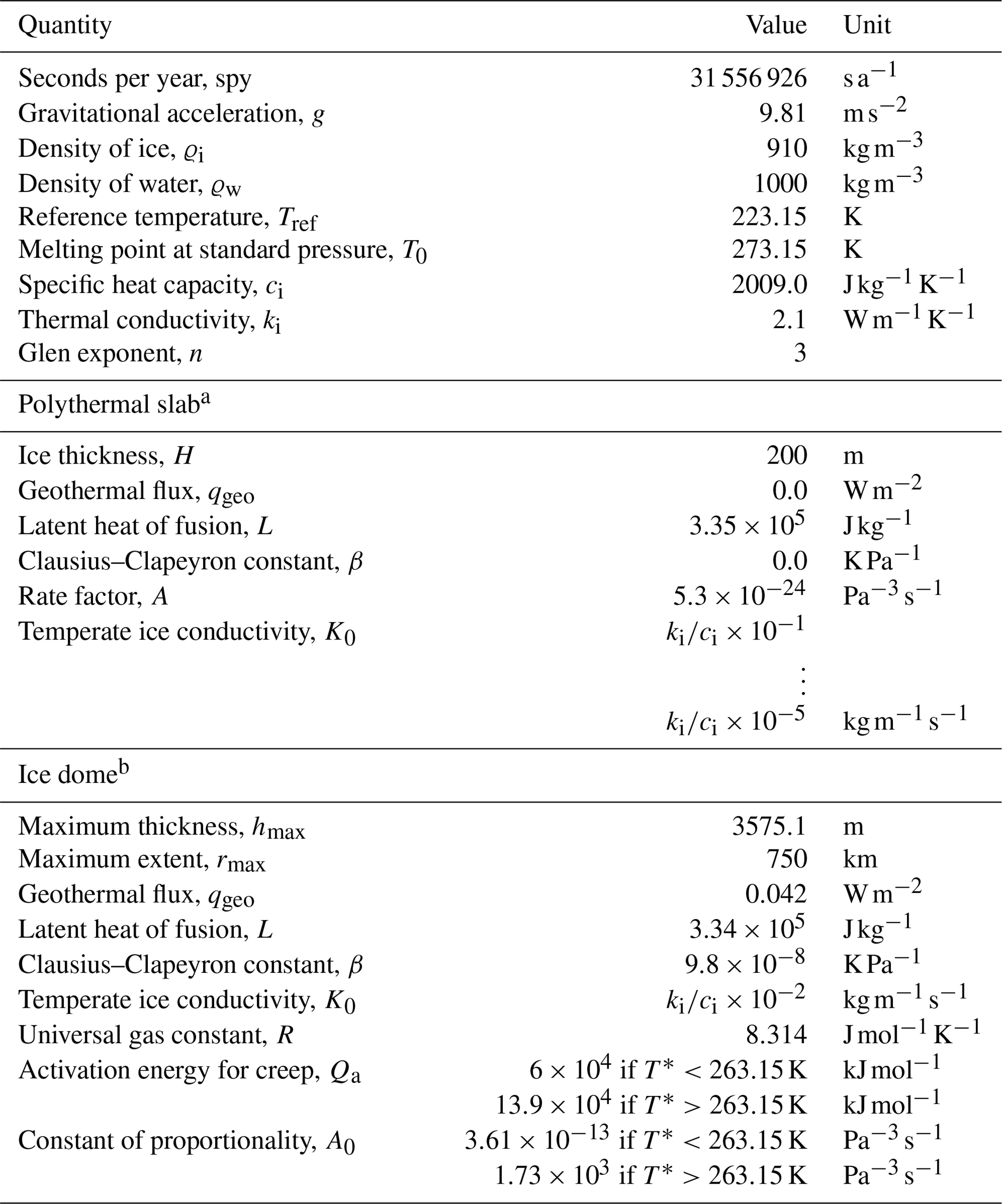
a Based on Greve and Blatter (2009). b Based on Vialov (1958) and Payne et al. (2000).
We ran several experiments with the emphasis on testing our modifications in ISSM regarding accuracy and regarding stability. The discontinuous conductivity treatments are verified against an analytical solution within a polythermal-slab experiment. As this experiment results effectively in a one-dimensional vertical experiment, it is not suitable to test the SUPG parameter choices. Therefore, we set up a synthetic second ice dome experiment with variations in the topography. Constants and model parameters used in the experiments are summarized in Table 1.
3.1 Polythermal slab
We repeat the well-established polythermal sided slab experiment proposed in Greve and Blatter (2009) and already applied to ISSM in Kleiner et al. (2015). The setup poses a representative situation in glacier modelling with an intra-glacial CTS. The model domain consists of a 200 m thick and 4∘ downward-inclined ice slab. The horizontal velocity vx is prescribed as an analytical expression (from 5 m a−1 at the base towards ≈ 38 m a−1 at the surface) and does not vary horizontally. The vertical velocity is set to be constant and equal to m a−1 while vy=0 m a−1. In addition, the geothermal flux is set to be zero during the model run so that the englacial strain heating is the only source of energy in the enthalpy balance equation.
An analytical solution for the steady-state enthalpy profile based on the solution of Greve and Blatter (2009) leads to a CTS elevation 18.95 m above the bed. In our experiments, the conductivity ratio K0∕Kc is varied from 10−1 to 10−5. The simulations are performed on equidistant horizontal layers using different vertical resolutions m. To be comparable to the ISSM results published in Kleiner et al., 2015) no stabilization is applied in this setup; i.e. the term S(E,w) in Eq. (6) is ignored. Please note that the analytical solution considers K0=0 . In this experiment, we apply a thermal steady-state solver (i.e. in Eq. 1). Comparisons of results when applying a transient solver or a steady-state solver revealed no difference in the steady-state enthalpy profile.
3.2 Ice dome
In this experiment, a more realistic setup than the polythermal-slab experiment is considered with a three-dimensional ice dome based on the Vialov profile (Vialov, 1958). Other settings and parameters are borrowed from the EISMINT Phase 2 benchmark (Payne et al., 2000). The surface zs and bedrock zb of the entire ice sheet are defined as
with the ice thickness h(x,y), the maximum ice thickness hmax, the radius , the maximum extent rmax, and the Glen exponent n. The summit of the ice dome is located at .
In this experiment, a thermo-mechanical coupling is considered. The Glen–Steinemann power-law rheology (Steinemann, 1954; Glen, 1955) is used for the deformation of ice. The ice viscosity reads
where A is the flow rate factor and the effective strain rate (regarded as the second invariant of the strain-rate tensor). A is assumed to be dependent on the temperature T* (temperature relative to the pressure melting point Tpmp) and liquid water fraction ω:
where A0 and are constants, Qa is the activation energy for creep, and R is the gas constant. The constant is equal to . The upper bound of the water fraction ω is 0.01 to ensure validity of the flow rate factor parameterization in the temperate part with the experimental dataset (Duval, 1977; Lliboutry and Duval, 1985).
For the dynamical model, we employ the higher-order Blatter–Pattyn approximation (Blatter, 1995; Pattyn, 2003). Basal sliding is allowed everywhere, and the basal drag, τb, is written as
where vb,i is the basal velocity component in the horizontal plane and and k2 the friction coefficient. The effective pressure is defined as N=ϱi g h. At the ice front a zero pressure boundary condition is applied as all the ice is above sea level. A traction-free boundary condition is imposed at the ice–air interface.
For the thermal model, we impose a Dirichlet condition at the surface:
The ice sheet base is subject to the decision chart presented in Aschwanden et al. (2012). In this implementation, the basal boundary condition is allowed to switch between Neumann and Dirichlet type depending on the thermal basal conditions. The geothermal flux, qgeo, is considered spatially constant.
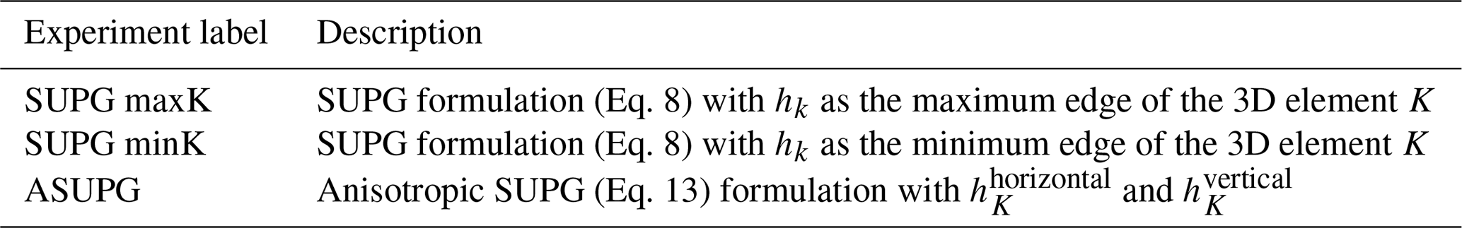
To investigate the sensitivity of over- and under-stabilization, we perform experiments with three different stabilization formulations (Table 2). The setup SUPG maxK is the standard SUPG setup based on the maximum edge length of an element K for the local mesh parameter hK. In contrast, the SUPG minK uses the minimum edge length as, however, recommended for anisotropic 2D meshes (Harari and Hughes, 1992; Mittal, 2000). Finally, the ASUPG is employed.
To study whether the stabilization is dependent on different mesh resolutions and the amount of advection, we vary the horizontal grid size and the amount of sliding. Here, we use a base mesh of 20 km in the interior, which is subsequently refined to towards the glacier margin. The friction coefficient is treated as spatially constant and several experiments are performed with . For the three sliding cases, this results in frontal velocities of about 50, 350, and 1100 m a−1, respectively. We use 15 layers refined close to the base to account for the high-velocity gradients and vertical shearing near the base in the vertical direction. The simulations are run 2000 years forward in time without necessarily reaching a steady state.
4.1 Polythermal slab
The final steady-state CTS elevations for all simulations are shown in Fig. 1. For the maximum value of temperate ice conductivity (), the models result in a CTS elevation around 36–39 m. With decreasing K0∕Kc, the temperate ice layer thickness consistently decreases for the harmonic and geometric mean models and is almost halved for the lowest conductivity ratio ; the solution converges to the analytical CTS elevation for the high mesh resolution. However, for the harmonic mean, we detect a larger spread over the grid resolutions at low K0∕Kc compared to the geometric mean. The simulations with the arithmetic mean yield a completely different picture. The range in the CTS elevation increases considerably with decreasing K0∕Kc, and the analytical CTS elevation is met for the highest mesh resolution, below 2 m.
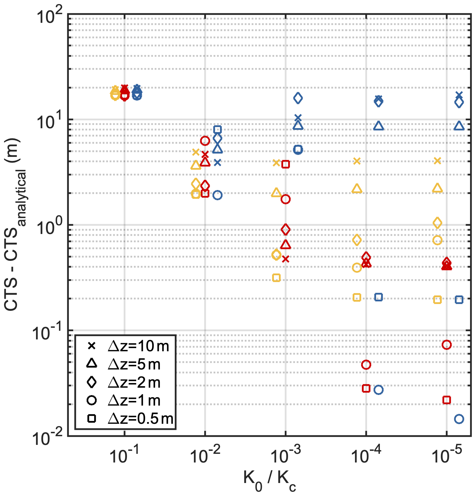
Figure 1Difference of simulated steady-state CTS elevations to the analytical CTS elevation for different values of the temperate ice conductivity, K0, for the polythermal-slab experiment. The analytical CTS elevation is 18.95 m. The different conductivity models are shown as harmonic mean (yellow), geometric mean (red), and arithmetic mean (blue). Results of different models are slightly shifted on the x axis so as not to overlay each other. The dashed black line indicates the CTS elevation of the analytical solution derived for .
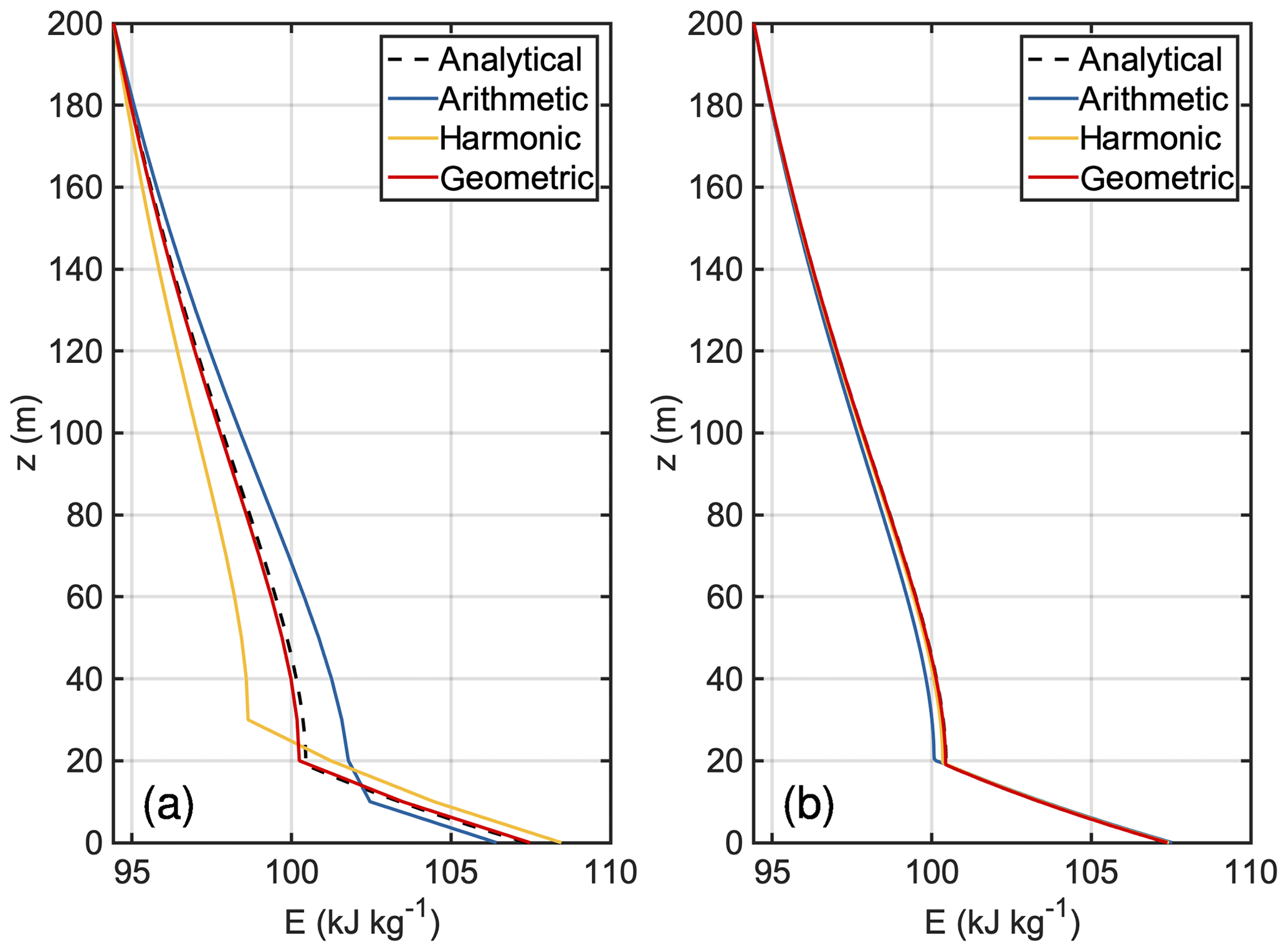
Figure 2Simulated steady-state profiles of the enthalpy E computed with the three conductivity models with and a vertical resolution of Δz=10 m (a) and Δz=0.5 m (b) compared to the analytical profile.
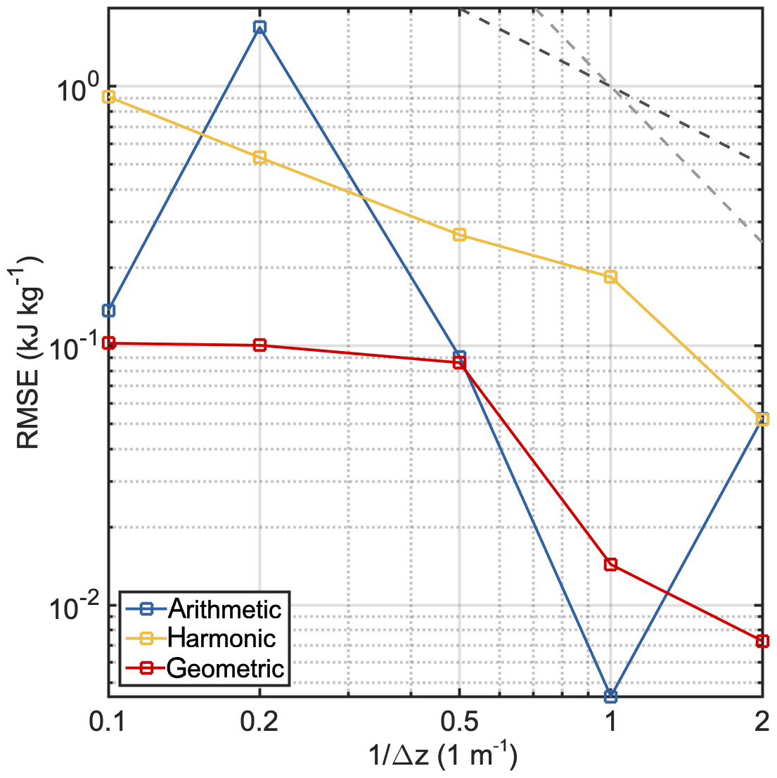
Figure 3Root-mean-square error (RMSE) for the polythermal-slab experiment. The RMSE is computed between the modelled enthalpy result and the analytical solution for different vertical grid resolutions Δz and for each conductivity parameterization. Model results are obtained for the lowest conductivity ratio . The dashed light and dark grey lines show the indicative rate for (Δz)1 and (Δz)2, respectively.
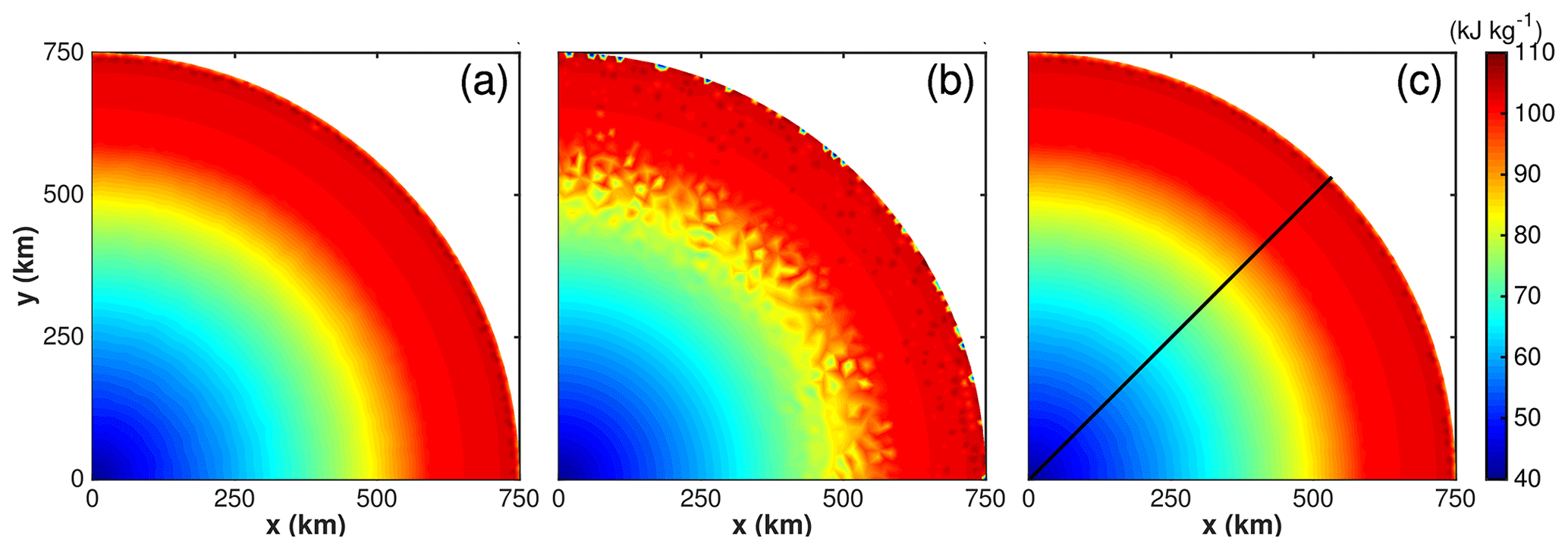
Figure 4Simulated enthalpy (kJ kg−1) for the ice dome experiment with lmin=10 km and . (a) SUPG maxK, (b) SUPG minK, and (c) ASUPG. Black line in (c) indicates the location of the cross section shown in Fig. 5.

Figure 5Simulated enthalpy (kJ kg−1) for the ice dome experiment with lmin=10 km and along a vertical cross section. (a) SUPG maxK, (b) SUPG minK, and (c) ASUPG. The location of the cross section is shown in Fig. 4c.
The steady-state results of the three conductivity models are verified with the analytical solution of the vertical enthalpy profile. Figure 2 shows the simulated vertical enthalpy profiles for Δz=10 and 0.5 m and the lowest conductivity ratio . The results of all models agree well with the analytical solution for high resolutions. At coarser resolutions, however, the simulated enthalpy profiles differ noticeably from the analytical solution for the arithmetic and the harmonic mean, while the geometric mean coincides well with the analytical solution. Please note that the results for the harmonic mean are similar to those presented in Kleiner et al. (2015) for ISSM.
The accuracy of the simulations with the lowest conductivity ratio is measured with the root-mean-square error (RMSE) to the analytical solution. The RMSE as a function of vertical resolution is shown in Fig. 3. All three models exhibit different behaviours. The arithmetic mean reveals a somewhat inconsistent behaviour, while the harmonic mean shows approximately first-order convergence as Δz→0. Overall, the geometric mean shows low errors, and the error remains on a similarly low level even for coarse resolutions.
The different behaviours highlight the dependency of the solution on the CTS implementation details. As already identified by Kleiner et al. (2015) the use of an arithmetic mean leads to oscillations in the enthalpy solution that are visible, e.g., in a time-varying CTS elevation. Consequently, no steady-state solution is reached under these conditions. Here, when applying a steady-state solver, the solver does not converge and the CTS elevation flips between the non-linear iterations.
4.2 Ice dome
In this experiment, we explore the impact of the parameter choices in the SUPG formulation on the reliability and accuracy of the results. In Fig. 4 the simulated basal enthalpy field is shown for the lowest resolution lmin=10 km and high sliding case for the three employed stabilization formulations. Due to symmetry, only the upper-right part of the domain is shown. As expected, the SUPG minK produces unphysical oscillations in the simulated enthalpy field. SUPG maxK and ASUPG reveal a smooth result with merely minor oscillations at the ice front, where the surface slopes become singular. The same picture is observed along a cross section of the ice sheet interior (Fig. 5). For the SUPG minK, the numerical oscillations in the enthalpy field are visible in the whole ice profile. The same qualitative behaviour among the SUPG formulations is detected for all employed grid resolutions and sliding cases (Fig. 6). Increasing the mesh resolution leads to a significant reduction in upstream oscillations. However, oscillations still occur close to the ice margin. This is in line with the theory that τk must vanish as grid refinement increases, and no stabilization may be necessary for sufficiently fine meshes. The amount of basal sliding, which controls the amount of advection, plays a secondary role.
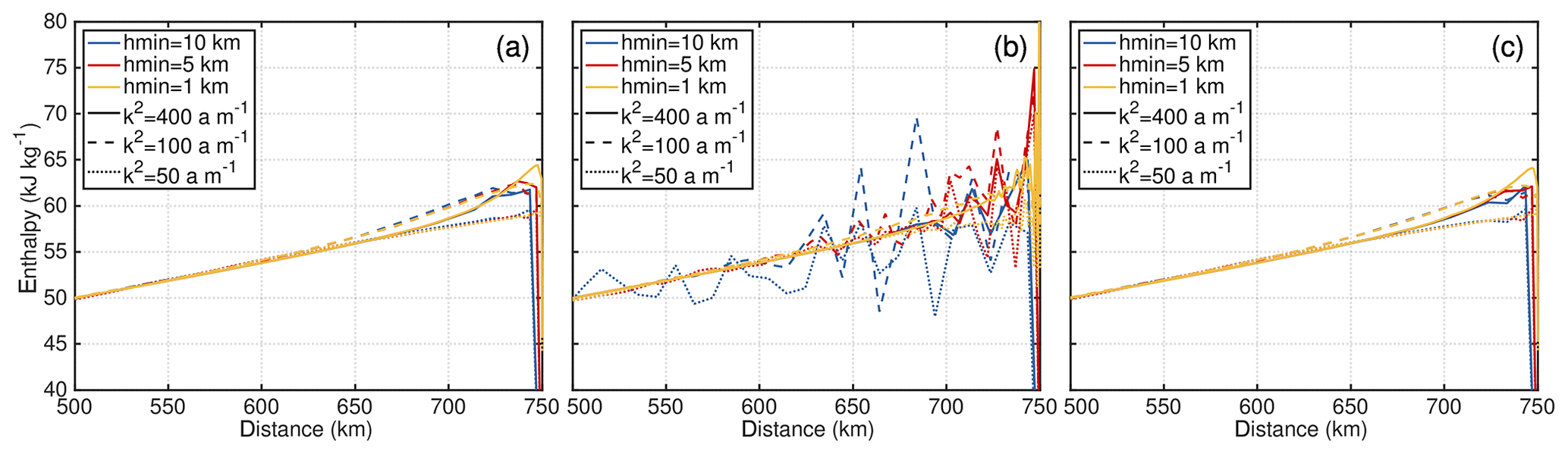
Figure 6Simulated depth-averaged enthalpy (kJ kg−1) for the ice dome experiment along a cross section. (a) SUPG maxK, (b) SUPG minK, (c) ASUPG. The location of the cross section is shown in Fig. 4c.
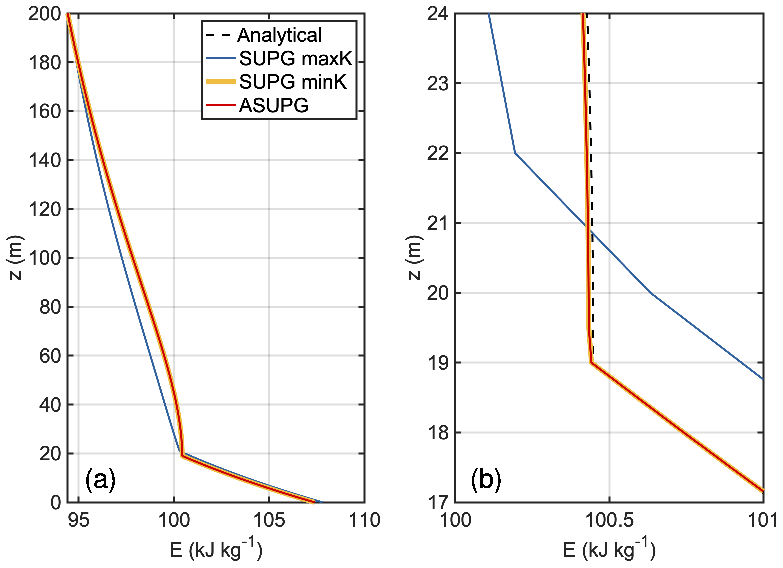
Figure 7Simulated steady-state profiles of the enthalpy E for the three different SUPG models by employing the geometric mean (Eq. 16) and a vertical resolution of Δz=0.5 m (a). Zoom to CTS region (b). Please note that ASUPG and SUPG minK overlay each other.
Surprisingly, SUPG maxK and ASUPG are visually indistinguishable and result in qualitatively similar results. However, when re-running the polythermal-slab experiment with the three SUPG formulations, distinct differences in the simulated enthalpy are obtained (Fig. 7). The simulations with ASUPG and SUPG minK both match the analytical solution with RMSE = 0.01 and 0.01 kJ kg−1, respectively. The simulation with SUPG maxK deviates considerably from the analytical solution with RMSE = 0.48 kJ kg−1. Overall, we find that (1) using SUPG maxK as the local mesh parameter results in an oscillation-free enthalpy field but tends to produce far more diffusion than the other choices, (2) using SUPG minK as the local mesh parameter results in unphysically large oscillations for more complex geometries, and (3) ASUPG provided realistic solutions in all conducted experiments.
Our results demonstrate that choosing the stabilization parameter in a heuristic or ad hoc manner, without knowledge of the possible effects, can impact the solution significantly. Choosing a sub-optimal value for the stabilization parameter can affect the accuracy of the solution and result in over- or under-stabilization. The viability of the SUPG formulation strongly depends on appropriate parameter choices, and in a worst-case scenario, the oscillations could cause unphysical values or the solver to diverge. However, we have not investigated how the solution differences propagate to other components of an ice sheet model, e.g. by coupling to the evolution of the ice thickness.
Since the above-presented solutions for the ASUPG method are excellent, the parameter choices for the local mesh parameters , , and the velocity norm are not further investigated. The velocity norm is here treated equally in both directions (Eq. 9), and no differentiation is made between the horizontal and vertical direction. Some test runs (not shown here) applying direction-dependent Euclidean norms of the velocity revealed no discernible differences to the above-presented results. Additionally, in the current implementation, the local mesh parameter in the horizontal direction, , does not cover anisotropy of elements in the horizontal plane. However, these simplifications have so far not led to numerical problems but might be subject to future work.
We presented extended enthalpy formulations within the ice flow model ISSM compared to Seroussi et al. (2013) and Kleiner et al. (2015). Treating the discontinuous conductivities at the CTS as a geometric mean results in a good solution for coarse resolutions compared to the analytical solution. This treatment is an improvement compared to earlier ISSM results presented in Kleiner et al. (2015) and based on a harmonic mean.
Additionally, we tested various SUPG stabilization formulations regarding their ability to deal with the high aspect ratio of 3D elements in glaciological applications. We found that the traditional parameters in the SUPG stabilization coefficients are susceptible to stabilization parameter choices, here the local mesh parameter, which is easily adjustable. We propose a novel anisotropic SUPG (ASUPG) method that circumvents the high aspect ratio problem in ice sheet modelling by treating the horizontal and vertical direction separately in the stabilization coefficients. The ASUPG method provides accurate results for the thermodynamic equation on geometries with very small aspect ratios like ice sheets.
The ice flow model ISSM version 4.17 (Larour et al., 2012) is open source and freely available at https://issm.jpl.nasa.gov/ (last access: 14 September 2020).
MR conducted the study supported by the other authors. MR set up the experiments conducted with ISSM and analysed the experiments. MM and HS provided technical ISSM support. MR wrote the paper together with the other authors.
The authors declare that they have no conflict of interest.
Martin Rückamp acknowledges support of the Helmholtz Climate Initiative REKLIM (Regional Climate Change). We thank Stephen Cornford and Alexander Robinson for the reviews that helped to improve the paper. For discussions and suggestions we thank Vadym Aizinger (University Bayreuth), Yonqi Wang (University Darmstadt), and Luca Wester (University of Erlangen).
The article processing charges for this open-access publication were covered by a Research Centre of the Helmholtz Association.
This paper was edited by Philippe Huybrechts and reviewed by Alexander Robinson and Stephen Cornford.
Aschwanden, A., Bueler, E., Khroulev, C., and Blatter, H.: An enthalpy formulation for glaciers and ice sheets, J. Glaciol., 58, 441–457, https://doi.org/10.3189/2012JoG11J088, 2012. a, b, c, d, e, f
Becker, R. and Rannacher, R.: Finite Element Solution of the Incompressible Navier-Stokes Equations on Anisotropically Refined Meshes, Vieweg+Teubner Verlag, Wiesbaden, 52–62, https://doi.org/10.1007/978-3-663-14125-9_4, 1995. a, b
Blasco, J.: An anisotropic GLS-stabilized finite element method for incompressible flow problems, Comput. Method. Appl. M., 197, 3712–3723, https://doi.org/10.1016/j.cma.2008.02.031, 2008. a, b
Blatter, H.: Velocity and stress fields in grounded glaciers: a simple algorithm for including deviatoric stress gradients, J. Glaciol., 41, 333–344, https://doi.org/10.3189/S002214300001621X, 1995. a
Blatter, H. and Greve, R.: Comparison and verification of enthalpy schemes for polythermal glaciers and ice sheets with a one-dimensional model, Polar Sci., 9, 196–207, https://doi.org/10.1016/j.polar.2015.04.001, 2015. a
Blatter, H. and Hutter, K.: Polythermal conditions in arctic glaciers, J. Glaciol., 37, 261–269, https://doi.org/10.3189/S0022143000007279, 1991. a, b
Brinkerhoff, D. J. and Johnson, J. V.: Data assimilation and prognostic whole ice sheet modelling with the variationally derived, higher order, open source, and fully parallel ice sheet model VarGlaS, The Cryosphere, 7, 1161–1184, https://doi.org/10.5194/tc-7-1161-2013, 2013. a
Brinkerhoff, D. and Johnson, J.: A stabilized finite element method for calculating balance velocities in ice sheets, Geosci. Model Dev., 8, 1275–1283, https://doi.org/10.5194/gmd-8-1275-2015, 2015. a
Brooks, A. N. and Hughes, T. J.: Streamline upwind/Petrov-Galerkin formulations for convection dominated flows with particular emphasis on the incompressible Navier-Stokes equations, Comput. Method. Appl. M., 32, 199–259, https://doi.org/10.1016/0045-7825(82)90071-8, 1982. a, b
Church, J. A., Clark, P. U., Cazenave, A., Gregory, J. M., Jevrejeva, S., Levermann, A., Merrifield, M. A., Milne, G. A., Nerem, R. S., Nunn, P. D., Payne, A. J., Pfeffer, W. T., Stammer, D., and Unnikrishnan, A. S.: Sea level change, in: Climate Change 2013: The Physical Science Basis. Working Group I Contribution to the Fifth Assessment Report of the Intergovernmental Panel on Climate Change, Cambridge University Press, 1137–1216, 2013. a
Duval, P.: The role of water content on the creep rate of polychristalline ice, International Association of Hydrological Sciences Publication, 118, 29–33, 1977. a, b
Feldmann, J. and Levermann, A.: From cyclic ice streaming to Heinrich-like events: the grow-and-surge instability in the Parallel Ice Sheet Model, The Cryosphere, 11, 1913–1932, https://doi.org/10.5194/tc-11-1913-2017, 2017. a
Fowler, A. C.: On the transport of moisture in polythermal glaciers, Geophys. Astrophys. Fluid Dynam., 28, 99–140, https://doi.org/10.1080/03091928408222846, 1984. a, b
Franca, L. P., Frey, S. L., and Hughes, T. J.: Stabilized finite element methods: I. Application to the advective-diffusive model, Comput. Method. Appl. M., 95, 253–276, https://doi.org/10.1016/0045-7825(92)90143-8, 1992. a
Franca, L. P., Hauke, G., and Masud, A.: Revisiting stabilized finite element methods for the advective–diffusive equation, Comput. Method. Appl. M., 195, 1560–1572, https://doi.org/10.1016/j.cma.2005.05.028, 2006. a, b, c
Ghanbarian, B. and Daigle, H.: Thermal conductivity in porous media: Percolation-based effective-medium approximation, Water Resour. Res., 52, 295–314, https://doi.org/10.1002/2015WR017236, 2016. a
Glen, J. W.: The Creep of Polycrystalline Ice, P. Roy. Soc. A-Math. Phy., 228, 519–538, https://doi.org/10.1098/rspa.1955.0066, 1955. a
Greve, R.: A continuum-mechanical formulation for shallow polythermal ice sheets, P. Roy. Soc. A-Math. Phy., 355, 921–974, https://doi.org/10.1098/rsta.1997.0050, 1997. a
Greve, R. and Blatter, H.: Dynamics of Ice Sheets and Glaciers, in: Advances in Geophysical and Environmental Mechanics and Mathematics, Springer, Berlin Heidelberg, https://doi.org/10.1007/978-3-642-03415-2, 2009. a, b, c, d, e
Greve, R. and Blatter, H.: Comparison of thermodynamics solvers in the polythermal ice sheet model SICOPOLIS, Polar Sci., 10, 11–23, https://doi.org/10.1016/j.polar.2015.12.004, 2016. a, b, c, d
Harari, I. and Hughes, T. J.: What are C and h?: Inequalities for the analysis and design of finite element methods, Comput. Method. Appl. M., 97, 157–192, https://doi.org/10.1016/0045-7825(92)90162-D, 1992. a
Helanow, C. and Ahlkrona, J.: Stabilized equal low-order finite elements in ice sheet modeling – accuracy and robustness, Comput. Geosci., 22, 951–974, https://doi.org/10.1007/s10596-017-9713-5, 2018. a
Hewitt, I. J. and Schoof, C.: Models for polythermal ice sheets and glaciers, The Cryosphere, 11, 541–551, https://doi.org/10.5194/tc-11-541-2017, 2017. a, b
Hindmarsh, R. C. A.: Consistent generation of ice-streams via thermo-viscous instabilities modulated by membrane stresses, Geophys. Res. Lett., 36, L06502, https://doi.org/10.1029/2008GL036877, 2009. a
Hoffman, M. J., Perego, M., Price, S. F., Lipscomb, W. H., Zhang, T., Jacobsen, D., Tezaur, I., Salinger, A. G., Tuminaro, R., and Bertagna, L.: MPAS-Albany Land Ice (MALI): a variable-resolution ice sheet model for Earth system modeling using Voronoi grids, Geosci. Model Dev., 11, 3747–3780, https://doi.org/10.5194/gmd-11-3747-2018, 2018. a
Hutter, K.: A mathematical model of polythermal glaciers and ice sheets, Geophys. Astrophys. Fluid Dynam., 21, 201–224, https://doi.org/10.1080/03091928208209013, 1982. a, b
John, V. and Knobloch, P.: On spurious oscillations at layers diminishing (SOLD) methods for convection-diffusion equations: Part I – A review, Comput. Method. Appl. M., 196, 2197–2215, https://doi.org/10.1016/j.cma.2006.11.013, 2007. a
John, V., Knobloch, P., and Novo, J.: Finite elements for scalar convection-dominated equations and incompressible flow problems: a never ending story?, Computing and Visualization in Science, 19, 47–63, https://doi.org/10.1007/s00791-018-0290-5, 2018. a, b
Jorand, R., Fehr, A., Koch, A., and Clauser, C.: Study of the variation of thermal conductivity with water saturation using nuclear magnetic resonance, J. Geophys. Res.-Sol. Ea., 116, B08208, https://doi.org/10.1029/2010JB007734, 2011. a
Kleiner, T., Rückamp, M., Bondzio, J. H., and Humbert, A.: Enthalpy benchmark experiments for numerical ice sheet models, The Cryosphere, 9, 217–228, https://doi.org/10.5194/tc-9-217-2015, 2015. a, b, c, d, e, f, g, h, i, j, k
Knobloch, P.: On the definition of the SUPG parameter, ETNA: Electronic Transactions on Numerical Analysis, 32, 76–89, 2008. a
Larour, E., Seroussi, H., Morlighem, M., and Rignot, E.: Continental scale, high order, high spatial resolution, ice sheet modeling using the Ice Sheet System Model (ISSM), J. Geophys. Res.-Earth, 117, F01022, https://doi.org/10.1029/2011JF002140, 2012. a, b, c
Lliboutry, L. and Duval, P.: Various isotropic and anisotropic ices found in glaciers and polar ice caps and their corresponding rheologies, Ann. Geophys., 3, 207–224, 1985. a
MacAyeal, D. R.: Binge/purge oscillations of the Laurentide Ice Sheet as a cause of the North Atlantic's Heinrich events, Paleoceanography, 8, 775–784, https://doi.org/10.1029/93PA02200, 1993. a
Midttømme, K. and Roaldset, E.: Thermal conductivity of sedimentary rocks: uncertainties in measurement and modelling, Geol. Soc. SP, 158, 45–60, https://doi.org/10.1144/GSL.SP.1999.158.01.04, 1999. a
Mittal, S.: On the performance of high aspect ratio elements for incompressible flows, Comput. Method. Appl. M., 188, 269–287, https://doi.org/10.1016/S0045-7825(99)00152-8, 2000. a, b
Nield, D. A. and Bejan, A.: Convection in Porous Media, in Convection Heat Transfer, John Wiley & Sons, Inc., Hoboken, NJ, USA, 4th edn., 2013. a, b, c, d, e
Patankar, S. V.: Numerical Heat Transfer and Fluid Flow, McGraw-Hill, New York, 1980. a
Pattyn, F.: A new three-dimensional higher-order thermomechanical ice-sheet model: basic sensitivity, ice-stream development and ice flow across subglacial lakes, J. Geophys. Res.-Sol. Ea., 108, 2382, https://doi.org/10.1029/2002JB002329, 2003. a
Payne, A., Huybrechts, P., Abe-Ouchi, A., Calov, R., Fastook, J., Greve, R., Marshall, S., Marsiat, I., Ritz, C., Tarasov, L., and Thomassen, M.: Results from the EISMINT model intercomparison: the effects of thermomechanical coupling, J. Glaciol., 46, 227–238, https://doi.org/10.3189/172756500781832891, 2000. a, b
Reddy, K. S. and Karthikeyan, P.: Combinatory Models for Predicting the Effective Thermal Conductivity of Frozen and Unfrozen Food Materials, Adv. Mech. Eng., 2, 901376, https://doi.org/10.1155/2010/901376, 2010. a, b
Seroussi, H., Morlighem, M., Rignot, E., Khazendar, A., Larour, E., and Mouginot, J.: Dependence of century-scale projections of the Greenland ice sheet on its thermal regime, J. Glaciol., 59, 1024–1034, https://doi.org/10.3189/2013JoG13J054, 2013. a, b, c, d
Steinemann, S.: Results of Preliminary Experiments on the Plasticity of Ice Crystals, J. Glaciol., 2, 404–416, https://doi.org/10.3189/002214354793702533, 1954. a
Tezduyar, T. E. and Osawa, Y.: Finite element stabilization parameters computed from element matrices and vectors, Comput. Method. Appl. M., 190, 411–430, https://doi.org/10.1016/S0045-7825(00)00211-5, 2000. a
Vialov, S. S.: Regularities of glacial shields movement and the theory of plastic viscous flow, Physics of the movements of ice, IAHS, 47, 266–275, 1958. a, b
Voller, V.: Numerical treatment of rapidly changing and discontinuous conductivities, Int. J. Heat Mass Tran., 44, 4553–4556, https://doi.org/10.1016/S0017-9310(01)00089-8, 2001. a
Voller, V. R. and Swaminathan, C.: Treatment of discontinuous thermal conductivity in control-volume solutions of phase-change problems, Numer. Heat Tr. B-Fund., 24, 161–180, https://doi.org/10.1080/10407799308955887, 1993. a
Wang, J., Carson, J. K., North, M. F., and Cleland, D. J.: A new approach to modelling the effective thermal conductivity of heterogeneous materials, Int. J. Heat Mass Tran., 49, 3075–3083, https://doi.org/10.1016/j.ijheatmasstransfer.2006.02.007, 2006. a, b