the Creative Commons Attribution 4.0 License.
the Creative Commons Attribution 4.0 License.
 | 23 Sep 2020
The E3SM version 1 single-column model
Peter A. Bogenschutz
Shuaiqi Tang
Peter M. Caldwell
Shaocheng Xie
Wuyin Lin
Yao-Sheng Chen
The single-column model (SCM) functionality of the Energy Exascale Earth System Model version 1 (E3SMv1) is described in this paper. The E3SM SCM was adopted from the SCM used in the Community Atmosphere Model (CAM) but has evolved significantly since then. We describe changes made to the aerosol specification in the SCM, idealizations, and developments made so that the SCM uses the same dynamical core as the full general circulation model (GCM) component. Based on these changes, we describe and demonstrate the seamless capability to “replay” a GCM column using the SCM. We give an overview of the E3SM case library and briefly describe which cases may serve as useful proxies for replicating and investigate some long-standing biases in the full GCM runs while demonstrating that the E3SM SCM is an efficient tool for both model development and evaluation.
- Article
(1744 KB) - Full-text XML
- BibTeX
- EndNote


Despite advances in computation allowing for general circulation models (GCMs) to be run with progressively finer resolution with each successive generation, the parameterized physics in the atmospheric components of these GCMs have steadily become more complex. Indeed, while this increase in complexity often leads to better climate simulations due to more realistic and comprehensive processes being accounted for, understanding interactions between these parameterizations and the GCM dynamics can be a daunting task. A tool to help GCM physics development and evaluation is the so-called single-column model (SCM) framework, which is a functionality that exists in many state-of-the-art GCMs. This work was pioneered by Betts and Miller (1986), with the link between SCMs, observations, and GCMs studied more extensively in Randall et al. (1996). An SCM is a mode where a single column of the atmosphere is run in isolation with prescribed atmospheric dynamics. Thus, the SCM will simulate unresolved processes within the atmospheric column, such as clouds, microphysics, turbulence, and radiation while removing the complexity of the dynamics–physics interactions.
SCMs are often the first step in the GCM parameterization development and/or implementation process. This is due to the fact that SCMs can provide a framework for quicker and easier debugging compared to the full GCM counterpart. In addition, depending on the regime of interest being targeted, the SCM simulation can readily be compared against observations or large eddy simulation (LES). This allows for rapid feedback of the parameterization performance in a more process-oriented environment. Park (2014) and Bogenschutz et al. (2012) are examples of how an SCM is used to implement and evaluate new and complex families of parameterizations in the National Center for Atmospheric Research's (NCAR's) Community Atmosphere Model version 5 (CAM5; Neale et al., 2012) SCM. The SCM can also be used as a tool to explore configurations that may not be feasible to do in a full GCM. For example, Bogenschutz et al. (2012) explored CAM, with two different physics packages, with very high LES-like vertical resolution that would have been computationally burdensome to do with a full GCM run. Smalley et al. (2019) use the SCM to construct a novel modeling framework that is forced by reanalysis to simulate a variety of environmental conditions in the subtropics to evaluate their parameterization suite.
SCMs are also useful tools for examining GCM physical parameterization performance at the process level. For instance, Zheng et al. (2017) used CAM's SCM to diagnose the cause of a cloudy planetary boundary layer oscillation, which was found to be the result of coupling issues between the turbulence and microphysics schemes. Zhang and Bretherton (2008) performed SCM studies to show that cloud feedbacks in CAM3 were controlled by unphysical oscillations caused by interactions between convection and resolved-scale processes. The SCM also provides a useful tool to perform perturbed parameter sensitivity studies for complex parameterizations that contain an abundance of tunable parameters, such as those performed by Guo et al. (2015).
The Energy Exascale Earth System Model version 1 (E3SMv1; Golaz et al., 2019) is an Earth system model designed with funding by the Department of Energy (DOE) for research and applications relevant to its mission. While E3SMv1 contains three new components (ocean, sea ice, and river) that have not previously been coupled to an Earth system model, the atmosphere and land components were branched from the Community Earth System Model version 1 (CESM1; Hurrell et al., 2013) but have evolved since (Xie et al., 2018; Rasch et al., 2019). Therefore, E3SMv1 inherited CAM and its associated SCM (Gettelman et al., 2019), but its SCM has also evolved. Those changes will be documented in this paper.
While SCMs have demonstrated that they are valuable tools for parameterization development, testing, and process-oriented evaluation efforts, they are unable to elucidate remote impacts or clarify physical–dynamical interactions where three-dimensional transport effects come into play. In addition, the SCM may replicate the behavior of the full GCM better for certain regimes and conditions than others, though this issue is poorly understood and not well studied. In this paper we will preliminarily demonstrate under what conditions the E3SM-SCM can serve as a useful proxy for GCM performance.
This paper is organized as follows: in Sect. 2 we describe the E3SM SCM and discuss modifications made to it since branching from CAM's SCM. The SCM case library is presented in Sect. 3, with links to documentation provided for users to assist in running the model. Section 4 describes the “replay” option, which allows the user to replicate a GCM column using the SCM for any point on the globe. Applications and examples of the SCM are presented in Sect. 5, including a preliminary analysis on when the SCM may serve as a useful proxy for the GCM and when it does not. Finally, a brief summary and discussion are presented in Sect. 6.
The E3SM Atmosphere Model version 1 (EAMv1; Xie et al., 2018; Rasch et al., 2019) was originally branched off from NCAR's CAM. Therefore E3SM inherited the CAM SCM (SCAM; Gettelman et al., 2019) and several similarities exist between the two.
Similar to SCAM, surface fluxes in E3SM can be prescribed and is the default setting if this information is available in the case forcing file. Otherwise, the surface fluxes are computed interactively via the land model or the data ocean model, using prescribed sea surface temperatures. The E3SM SCM does not currently support running an interactive ocean model, such as the work presented in Hartung et al. (2018), which may be a useful framework towards understanding parameterization feedbacks and climate sensitivity.
Section 2.1 through 2.3 focus on how the E3SM SCM was modified from the inherited CAM SCM.
2.1 Aerosol specification
The E3SM uses a prognostic modal aerosol model (Liu et al., 2016). While this represents a sophisticated and modern treatment of aerosol in E3SM, it presents challenges for an SCM and has been noted in Lebassi-Habtezion and Caldwell (2015) (hereafter LHC2015). Chief among these is the fact that E3SM initializes all aerosol mass mixing ratios to zero and results in unrealistically low aerosol concentrations until surface emissions loft sufficient aerosol. This is a process that can take several days to spin up (Schubert et al., 1979) and can significantly impact the simulated results of several SCM cases that are only hours in duration. LHC2015 show that CAM5 simulations are very sensitive to the initialization of aerosol for stratiform boundary layer cloud cases but not for shallow and deep convective cases (because deep and shallow convective microphysics schemes were not tied directly to the aerosol scheme). However, E3SM uses a unified treatment of shallow convection and planetary boundary layer turbulence (Golaz et al., 2002; Bogenschutz et al., 2013). Therefore, the shallow convective clouds are tied to the large-scale microphysics scheme and could lead to more severe impacts and sensitivities for the shallow and deep convective cloud regimes if aerosol is not specified adequately.
We have implemented the three options proposed by LHC2015 to initialize aerosol in the E3SM SCM. The first option is to use prescribed aerosol climatology derived from a 10-year E3SM present-day simulation with climatologically prescribed sea surface temperatures (SSTs). The second option is to specify the droplet and ice concentrations in the microphysics, thus bypassing the aerosol–cloud interaction, and the third option is to use observed aerosol information from the intensive observation period (IOP) forcing file if it is available. Selecting an aerosol specification option is mandatory for the E3SM SCM and a runtime error will result if a user attempts to run the SCM with no aerosol specification. For the scripts provided in the E3SM SCM case library (see Sect. 3), the most appropriate aerosol specification is already set for each particular case. Should an E3SM user generate their own forcing and is unsure which option to select, we advise using the prescribed aerosol specification as a default.
2.2 Idealizations
Many published LES comparison studies involving the simulation of boundary layer clouds include “idealizations”. As an example, the goal of the LES intercomparison study of the Barbados Ocean and Meteorological experiment (BOMEX; Holland and Rasmusson, 1973) was to investigate the role of turbulence dynamics for the shallow cumulus boundary layer (Siebesma et al., 2003) while avoiding the complications of microphysics and radiation. As such, none of the LESs participating in the study included a microphysical parameterization in their simulation. In addition, the radiative heating tendencies for the LES comparison were included in the large-scale forcing. Should an E3SM SCM user wish to evaluate the turbulence and cloud structure of the BOMEX case against the LES intercomparison study of Siebesma et al. (2003), not only would an apples-to-apples comparison not be possible with an out-of-the-box configuration of the inherited SCM, but it would also be scientifically invalid due to the fact that radiative tendencies would be double counted. While implementing these idealization switches into the model code is rather trivial, it is not an obvious task for the typical SCM user who is not familiar with the code and who may not be aware of the idealizations needed to match LES results.
Therefore, with the goal of preventing improper case setups, we have implemented idealization switches into the E3SM SCM code to allow for apples-to-apples comparison with IOP forcings corresponding to the appropriate reference for the particular case (see Sect. 3). The idealization switches added to the E3SM SCM framework include idealizations related to turning off microphysics and radiation calculations. All relevant switches have been added by default to the run scripts for each particular case but can be easily switched off by the user if they wish to examine that case using all E3SM physical parameterization schemes.
2.3 Consistent dynamical core
The code required to run the CAM SCM has long been entangled with the Eulerian dynamical core. As a result, the SCM could not be run with CAM's current Finite Volume (FV; Lin and Rood 1997; Neale et al., 2012) dynamical core or E3SM's spectral element (SE; Dennis et al., 2012) dynamical core. This is a problem because while the horizontal advection fields are provided by the IOP forcing files, the dynamical core is still responsible for computing the large-scale vertical transport if this is not prescribed in the forcing file. In the E3SM/CAM SCM the only part of the dynamical core that is exercised is the computation of the large-scale vertical transport. The Eulerian and SE dynamical cores use two different methods for this computation: the former uses a simple Eulerian calculation, while the latter uses a semi-Lagrangian method. Therefore, the inherited SCM was inconsistent with the full GCM with regard to how the large-scale vertical advection was computed. In addition, there are differences in the numerics between the two dynamical cores; whereas the Eulerian core uses a leapfrog numerical scheme, the SE dynamical core uses a third-order five-stage explicit Runge–Kutta (RK) method as described in Dennis et al. (2012). This results in different coupling between the prescribed and computed dynamical forcing with the physics and results in different dynamics and physics time steps between the SCM and the GCM run, which could cause inconsistencies between the two configurations if a particular parameterization scheme is sensitive to time step.
Ideally, we want the SCM to be as close a proxy to the full GCM run as possible. Thus we upgraded the SCM dycore to use the same SE dynamical core used by E3SM. Even though horizontal advection is prescribed in the SCM, the dycore still plays an important role for vertical advection. As described in Dennis et al. (2012), the SE dycore operates on quadrilateral elements whose Gauss–Lobatto–Legendre (GLL) quadrature points form the physics columns targeted by the SCM. Because there are many physics columns within each spectral element, it is impossible to initialize a single physics column when running a SE-dycore SCM. In this context the simplest way to initialize the SCM dycore is to “trick” the model by initializing the dynamical core using a low-resolution global configuration but then only actually use a single physics column for our calculations. We do this using the lowest-resolution configuration supported by E3SM, which contains 96 elements and corresponds to a grid spacing of approximately 7.5∘ at the Equator. Our strategy requires slightly more memory (to initialize the whole dynamics grid) but no more computational expense than if we initialized just one column (because we only perform physics and vertical advection calculations on a single column). This was the main challenge towards being able to use the SE dynamical core in the SCM setting, after which we trained the SE dynamical core to only calculate the large-scale vertical advection (i.e., no horizontal advection) in the column of interest if in SCM mode.
The E3SM SCM library is currently comprised of 25 cases that range from widely used cases of idealized boundary layer cloud regimes of a few hours in duration to unique cases that span the duration of years to a decade (i.e., continuous forcing from Atmospheric Radiation Measurement (ARM) Southern Great Plain (SGP) site; Xie et al., 2004). The list of available forcing files and their references can be found in Tables 1 and 2. Cases such as DYCOMS, BOMEX, MPACE, RICO, and ATEX are boundary layer cloud cases that are typically used to examine the performance of boundary layer, microphysics, and shallow convective parameterizations, while cases such as ARM97, ARM95, TWP (tropical west Pacific), and GATE are cases that can be used to evaluate shallow and deep convective parameterizations. The E3SM SCM library contains IOP files from more recent and modern cases, such as GOAMAZON, RACORO, and DYNAMO; many of these are unique to the E3SM SCM.
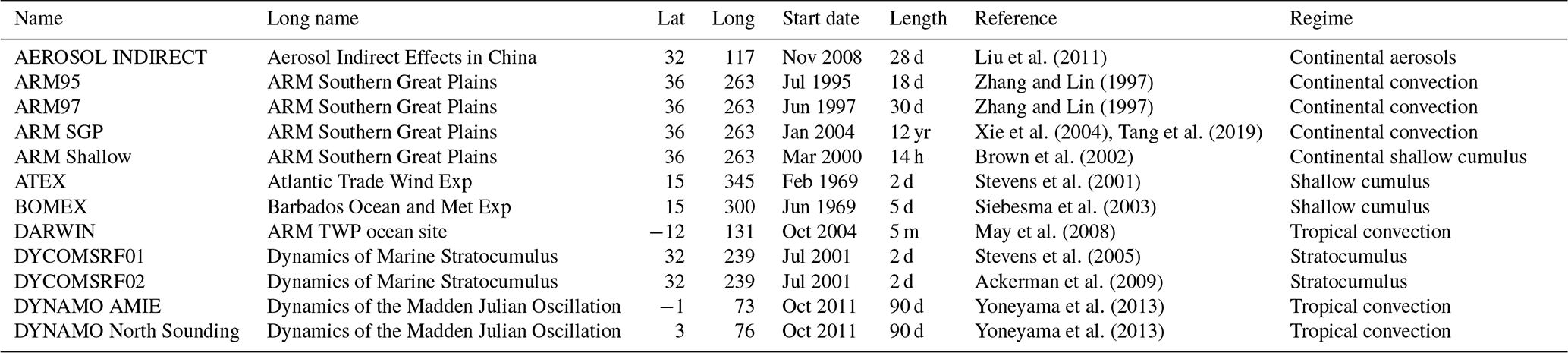
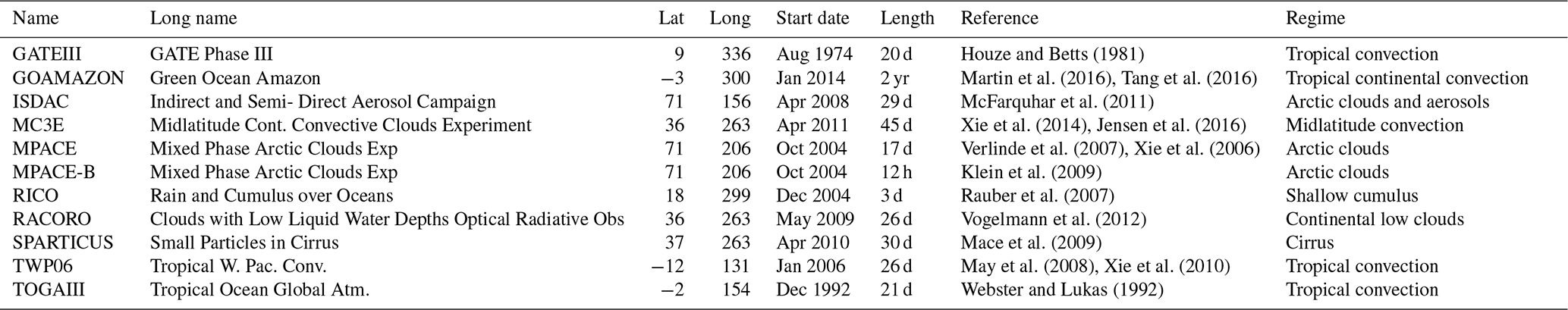
The E3SM SCM case library is publicly available on the E3SM SCM GitHub project wiki (https://github.com/E3SM-Project/scmlib/wiki/E3SM-Single-Column-Model-Case-Library, last access: 3 March 2020). The SCM user needs only to clone the GitHub repository that includes the scripts required to run the SCM cases. Note that the code needed to run the E3SM SCM is included with the standard E3SM release code. The user then needs to modify the header of the script for the desired case they wish to perform and then execute the script, which will compile and run the SCM for the desired case. We chose to provide and maintain separate scripts for each particular case, with the unique settings, switches, and idealizations for each case set in the script. An alternative approach is to provide the user with a universal script that can be used to run all cases and to hardcode each case into the E3SM infrastructure as a particular run type (known as a “compset” in the CAM/E3SM parlance). We find that providing unique scripts for each case provides more transparency, while the details of compsets tend to remain under the hood to most E3SM users. Our approach also provides the user with more flexibility to switch specific idealizations or settings on/off, allowing them to perform sensitivity studies. Cases in the E3SM library that include idealizations turned on by default include ATEX, BOMEX, DYCOMSRF01, DYCOMSRF02, MPACE-B, ARM shallow cumulus, and RICO. The remaining cases have no idealizations.
A major advantage of the SCM using the same dynamical core as the full GCM is the ability to easily replay a single GCM column to replicate a specific GCM column with only round-off error differences. This is a powerful tool, where the user generates IOP forcing from a full E3SM run, with the intention to replicate a column of interest in SCM mode. This can be used to help diagnose model crashes due to unstable physics parameterizations or to target and address chronic model biases in an efficient manner. It can also help to fill in the gap for a particular regime or location where there is no forcing provided by the E3SM SCM library. The inherited SCM, which used the Eulerian dynamical core, required additional post-processing of the GCM forcing to be compatible with the replay option (as documented in Gettelman et al., 2019), since forcing terms between the two dynamical cores are somewhat different. Since the E3SM SCM uses the same dynamical core as the full GCM, the method to replay a GCM column is straightforward and accurate.
Though the E3SM SCM replay option is accurate, it cannot provide a fully bit-by-bit representation of a GCM column. This is because the GCM and SCM will only give bit-by-bit answers if they do exactly the same calculations. In GCM mode, the end of the dynamics state is computed via a series of sub-stepped loops. For the SCM, the net effect of these loops must be encapsulated by the end-of-step values minus the beginning-of-step values, divided by the time step. This tendency is then added to the SCM state using forward Euler time stepping. Since the GCM and SCM calculations are not identical, roundoff level differences occur. This issue could in principle be resolved using quadruple precision output but we found the related difficulties associated with this to not be worth a roundoff level gain. Our approximate method has proven suitable for most scientific applications of interest to E3SM users. In Sect. 5.5, we demonstrate an example of using the replay option.
In this section we will demonstrate that the SCM can serve as a tool to reproduce and explore climatological biases within the E3SM. We will also show an example of when the SCM cannot be used as a proxy for the full model. Finally, we will show an example of using the E3SM replay option. Some major biases in the E3SM include (but are not limited to) an overestimate of clouds in the Arctic, lack of subtropical maritime stratocumulus, lack of high clouds in the TWP warm pool, timing of precipitation in the tropics and midlatitudes, and a lack of precipitation over the Amazon rainforest (Xie et al., 2018; Zhang et al., 2019; Golaz et al., 2019; Rasch et al., 2019). In this section we will attempt to replicate a select number of these biases with the SCM.
Unless otherwise stated, the SCM results presented in this paper use the short-term hindcast approach (Ma et al., 2015). The SCM is initiated every day at 00:00 Z and run for 2 d, with prescribed large-scale forcing and surface turbulent fluxes and without temperature and moisture profiles being nudged to observations. The 24 to 48 h forecasts in each simulation are then combined as a continuous time series. With the hindcast approach, the model is well constrained by the large-scale condition, allowing us to isolate problems related to parameterizations. It also avoids the possible impacts of nudging to the clouds and precipitation (Ghan et al., 2000; Zhang et al., 2014). For example, Randall and Cripe (1999) extensively discussed the nudging method for SCMs and conclude that the impact of nudging on SCM simulation depends on the model biases produced without nudging; thus there is no solid theory on what can be expected from a particular model while using nudging. We will, however, explore the differences between nudging and the short-hindcast mode in one example.
5.1 Diurnal cycle of continental precipitation
SCMs are a useful tool to explore biases due to the model's physical parameterizations. But are there certain conditions and regimes under which the SCM is a better or worse proxy for the full GCM? While it has been demonstrated many times in the literature (e.g., Golaz et al., 2002; Bogenschutz and Krueger 2013; Suselj et al., 2013) that boundary layer cloud cases (such as DYCOMS for stratocumulus and BOMEX for shallow cumulus, as an example) can serve as a useful surrogate to explore and improve biases in the global model (due to the important cloud-forming processes in these regimes being mostly locally driven), the question of whether precipitation due to deep convective processes can be replicated faithfully in SCMs is less understood. Here we will attempt to replicate E3SM's biases in precipitation, both in the mean state and variability sense, to see when the E3SM SCM may be useful to exploit and investigate these biases.
The diurnal cycle of precipitation, especially over land, is a mode of climate variability that GCMs have long struggled to simulate adequately (Covey et al., 2016; Lee et al., 2007). Over land the late afternoon peak in precipitation is typically associated with the transition of shallow to deep convection, while the nocturnal peak is mostly due to elevated convective systems associated with eastward-propagating mesoscale convective systems. Many studies have attributed the GCMs' inability to represent the diurnal cycle of precipitation to deficiencies in the moist convective parameterizations (Dai and Trenberth 2004; Lee et al., 2008), where model errors over land are associated with unrealistic strong coupling of convection to the surface heating (Lee et al., 2007; Xie et al., 2002). Thus, precipitation peaks in the model tend to occur too early over land during the day, especially in summer.
E3SMv1 strongly exhibits these aforementioned biases (Xie et al., 2019; hereafter XIE2019), especially when focused over the continental United States (CONUS; Fig. 9 of XIE2019). In the central plains of the US, observed precipitation peaks in the late evening time, whereas E3SM precipitation peaks around noon. Can E3SM SCM reproduce this bias and can we use the SCM to implement modifications to the parameterized physics that would help improve this long-standing issue? For this experiment we use version 2 of continuous forcing from the Southern Great Plains (SGP) ARM site (Tang et al., 2019; Xie et al., 2004) that spans from 2004 to 2015; however for this study we only consider the warm season from 1 May through 31 August of each year. Note that multi-year SCM forcing allows us to perform robust statistical analysis rather than relying on a single case study as typically done in the past with SCM runs.
To see if we can improve this bias in the SCM, we implemented a revised convective triggering function, as implemented in XIE2019, that has been shown to greatly improve the diurnal cycle of precipitation in E3SM simulations. This new convective triggering is a combination of two methods, known as dynamic convective available potential energy (dCAPE) and the unrestricted launch level (ULL).
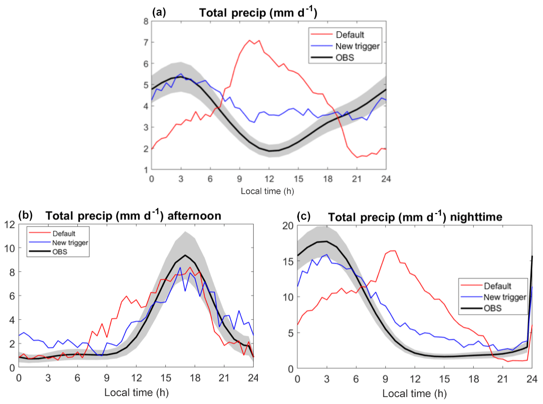
Figure 1Composite of the total precipitation (convective + large scale) in local time for the E3SM SCM (red curve), E3SM SCM with the convective modifications documented in Xie et al. (2019; blue curve), and observations (black curve) from the Southern Great Plains (SGP) ARM site version 2. Panel (a) depicts all time samples from 1 May through 31 August from 2004 to 2015. Panel (b) represents periods when the observed precipitation has a peak greater than 1 mm d−1 between 13:00 and 20:00 LST and when the peak rain rate is 1.5 times greater than any rain rate outside of 13:00 to 20:00 LST. Panel (c) represents periods when the observed precipitation is greater than 1 mm d−1 with a peak time between 00:00 and 07:00 LST.
Figure 1a displays the composite of the total precipitation from the periods sampled at the SGP site. While observations show a minimum of precipitation around noon, this is when E3SM SCM shows a maximum precipitation rate. This is representative of the bias found in E3SM simulations for a similar location over the North American Plains subset region in XIE2019, where precipitation was tied a bit too closely to solar insolation and the nocturnal peak in precipitation was not represented. XIE2019 also found that after implementing the revised dCAPE and ULL triggering method the precipitation maximum was shifted to the nocturnal hours (Fig. 13b of XIE2019). Clearly, not only can the E3SM SCM replicate the original bias found in the global model, but the improved representation due to the new convective triggering is also depicted in our SCM experiments.
Due to the fact that the SCM can replicate the behaviors seen in the global model for this situation, we can further use this SCM case to explore the exact reason for this behavior. Figure 1b and c conditionally sample our dataset for days when the observed precipitation predominately happens in the afternoon and nighttime. We segregate the days with afternoon maximum precipitation by subsetting to days when the observed precipitation has a peak greater than 1 mm d−1 between 13:00 and 20:00 LST and when the peak rain rate is 1.5 times greater than any rain rate outside of 13:00 to 20:00 LST. The nighttime precipitation days are classified as when the rain peak is greater than 1 mm d−1 with a peak time between 00:00 and 07:00 LST. From this analysis, it is clear that the largest impacts from the improved triggering in terms of precipitation timing occur on days when there is a nocturnal peak in precipitation and that the default E3SM was missing. The combination of the dCAPE trigger, which prevents the convection scheme from activating too early in the afternoon, and the ULL method, which improves the elevated nocturnal convection helps to shift the precipitation to the nighttime hours, on days when it is observed. Thus, this case makes an example of when the SCM can serve as a good proxy to replicate and improve GCM biases, as well as easily investigating under what scenarios an improved scheme is having the most impact.
5.2 Amazon precipitation bias
Another major bias in E3SM that is characteristic of most GCMs is the lack of precipitation over the Amazon (Fig. 9 of Xie et al., 2018). E3SM has a climatological dry bias upwards of 4 mm d−1 in this area that, while not as severe as most GCMs, is a long-standing bias that negatively impacts feedbacks to/from the land model. To see if we can replicate this bias in the E3SM SCM we use the Green Ocean Amazon (GOAMAZON) case (Table 1), which is a 2-year campaign taking place around the urban region of Manaus in central Amazonia from 2014 to 2015.
Figure 2a displays the annual cycle of precipitation for the SCM, observations, and the column closest to the GOAMAZON point for the E3SM GCM. Similarly, Figure 2b displays a composite of the daily cycle of precipitation. For this location, the radar-derived precipitation rate has an annual mean of 6.56 mm d−1, the SCM an annual mean of 6.98 mm d−1, and the GCM 6.07 mm d−1. Therefore, here we see an example where the SCM does not faithfully represent the bias exhibited by the GCM in terms of the climatological rate of precipitation. In fact, the SCM produces an excess of precipitation, although the early onset of precipitation bias seen in the GCM is also replicated by the SCM.
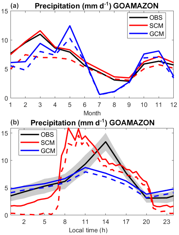
Figure 2Precipitation from the GOAMAZON field campaign for SCM (red curve) and observations (black curve). The GCM results (blue curve) are taken from an E3SM run in the column closest to the GOAMAZON location (3∘ S and 300∘ E) from January through December of 2014. Panel (a) represents the annual cycle of precipitation, while panel (b) represents the daily cycle. Solid curves represent the total precipitation rate, while dotted curves represent the contribution of the convective precipitation.
The reasoning why the GCM Amazon dry bias cannot be replicated in the SCM is likely because this bias is primarily due to a misrepresentation of the large-scale environmental conditions in the GCM rather than by parameterized deficiencies. This is important information for E3SM developers and the analysis team. Figure 3 displays the observed composite large-scale vertical velocity, relative humidity, and winds at the GOAMAZON location and compares these to the GCM simulated variables. The largest differences in the composites of large-scale vertical velocity and relative humidity between GCM and observations occur during the boreal summer months and correlate to the period of the most pronounced bias in the climatological rain rate in the GCM. The SCM is driven by observed large-scale forcing; thus it is not subject to the errors in the large-scale forcing that drives the E3SM dry Amazon bias.
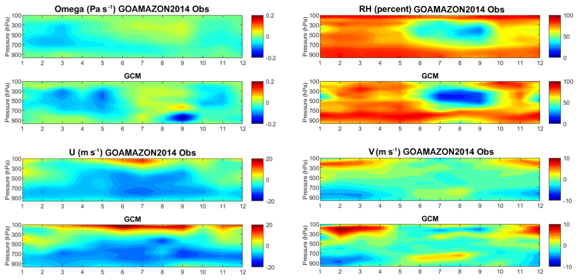
Figure 3Annual cycle of observed versus E3SM simulated environmental states for the GOAMAZON location for large-scale vertical velocity (top two left panels), relative humidity (top two right panels), zonal wind (bottom two left panels) and meridional wind (bottom two right panels).
In addition, it is well understood that for deep-convection precipitation is usually balanced mainly by advective moisture convergence, which is prescribed in these experiments. Therefore, this is a prime example of a situation where the SCM is not a useful tool to help improve GCM biases, but it does suggest that efforts should be spent on improving the large-scale circulation, or remote biases, that are probably responsible for the Amazon precipitation bias. As already mentioned, the SCM can replicate the bias related to the early onset of precipitation (similar to that seen in Fig. 1), thus supporting the idea that the diurnal cycle involves shorter timescales and therefore looks more like the free-running GCM solution than the observed values.
Having comprehensive a priori knowledge on what particular biases and regimes could faithful be replicated within an SCM framework would be invaluable for GCM development and improvement. However, this is currently poorly understood and should be the subject of future work.
5.3 Arctic clouds
Zhang et al. (2019) show that E3SM suffers from an overestimate of Arctic clouds, mostly in the form of too much liquid cloud. Here we use the Mixed-Phase Arctic Cloud Experiment (MPACE; Verlinde et al., 2007) case that sampled clouds over open ocean near Barrow, AK, with the goal to collect observations to advance the understanding of the dynamics and microphysical processes of mixed-phase clouds. This is a 17 d case taking place in October 2004.
The top row of Fig. 4 displays the cloud fraction from observations and from the E3SM SCM. The bottom row shows the time series of the liquid water path (LWP) and ice water path (IWP) for observations (black curve) and the default E3SM SCM in hindcast mode (red curve). As found in the GCM, we see a general overestimate of the cloud fraction in the E3SM SCM and a tendency for the E3SM SCM to overestimate LWP. This is in agreement with Zhang et al. (2019), who show a bias in the low-level cloud amount (their Fig. 3) and a negative shortwave cloud radiative effect bias in the Arctic. As described in Caldwell et al. (2019) this behavior is related to mistakenly setting the efficiency of the Bergeron–Findeisen process, in which ice crystals grow through sublimation at the expense of supercooled water droplets to the very low value of 0.1 in the v1 release. To test the impact of this choice, we set the Bergeron efficiency to 1.0. The result is a dramatic decrease in the amount of cloud liquid mixing ratio (third row of Fig. 4 and blue curve of bottom row). This example illustrates the ease with which the SCM can be used to explore the impact of parametric assumptions. Note, however, that this quick SCM test may not always capture the sensitivity of the full GCM, and our quick test does not account for needed retuning to compensate for altered Bergeron efficiency. However, how E3SM simulations would respond in the climatological sense and what degree of retuning would be necessary by adjusting this efficiency parameter is something that the SCM cannot provide insights on.
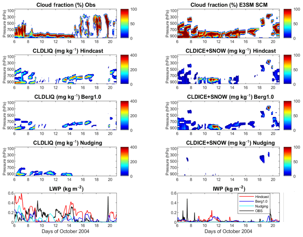
Figure 4Top panel displays the evolution of the vertical cloud structure for cloud fraction (observations on the left and E3SM SCM on the right) for the MPACE case from October 2004. The second through fourth panels on the left column represent the cloud liquid mixing ratio, while the second through fourth panels of the right column represent cloud ice mixing ratio from E3SM SCM simulations). The second row represents simulations using the hindcast method, the third row represents simulations with the Bergeron–Findeisen process set to the default tuning value, and row four represent the simulations where temperature and moisture are nudged to observations. The bottom row displays the evolution of the integrated liquid (left) and ice (right) path for the various configurations mentioned.
5.4 Hindcast vs. nudging
As previously mentioned, we chose to perform the majority of experiments in this paper in short-term hindcast mode. However, the E3SM SCM also comes with an option to nudge temperature and moisture to observed values. By default the E3SM SCM uses a nudging timescale of 3 h. It is interesting to note that the solution obtained for the MPACE case is strongly dependent on the technique used to constrain the mean state. The fourth row of Fig. 4, which uses nudging, clearly shows a very different solution in terms of the cloud and ice mixing ratio when compared to the hindcast simulation in the second row. The simulation with nudging tends to produce less liquid cloud and virtually no ice.
Figure 5 displays the time series of the observed temperature profiles for the MPACE period, in addition to the temperature biases for the E3SM SCM runs using hindcast and nudging methods. Obviously, since the nudged run is continually forced towards observations, the temperature bias is near zero for the duration of the run. Conversely, the hindcast run allows the temperature biases to grow over each 48 h run and is therefore likely to be more representative of the E3SM bias and therefore provide a more faithful representation of the model. This begs the question of which method should be used for E3SM SCM simulations. The answer likely depends on the goal of the particular user. If one simply wants to use the SCM as a proxy for E3SM performance, to replicate GCM biases and provide potential fixes for these biases, then running the SCM in short-term hindcast or free-running mode (for short IOP cases) is likely the best option. This will allow the mean state model biases to evolve, but not drift, in a manner similar to the GCM and will likely provide a more faithful representation in terms of cloud representation.
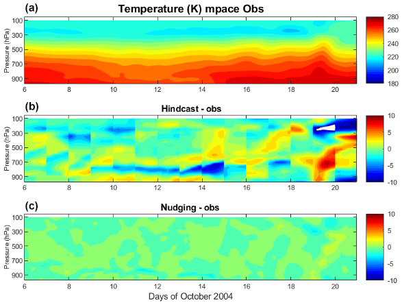
Figure 5Vertical evolution of temperature from observations (a) for the period during the MPACE field campaign. Also displayed are the temperature biases for the E3SM SCM run in hindcast mode (b) and for E3SM SCM run with nudging (c).
If, however, one is using the SCM for the purposes of parameterization development/implementation and wishes to assess their new parameterization in conditions with little to no mean state bias (e.g., to avoid compensating errors), then the nudging method is likely preferable. For instance, the results seen using nudging vs. hindcast for MPACE clouds may suggest that Arctic clouds simulated in E3SM are an artifact of compensating errors. When the observed temperature and moisture profiles are used, we see the model struggles to produce any ice cloud at all and is in conflict with observations. This suggests that E3SM developers may need to reevaluate either the parameterizations and/or tuning choices in order to get a desirable solution when the temperature and moisture most resemble observations. In addition, caution is warranted when using nudging, since constantly nudging to the observed temperature and moisture state inherently breaks the water and energy budget by acting as an artificial source. The sequential splitting techniques that E3SM uses could in theory be obscuring the direct effects of this and could be leading to the artificial reduction in condensate. However, this idea needs to be explored more.
5.5 Example of using the E3SM SCM replay option
Xie et al. (2018), Golaz et al. (2019), and Zhang et al. (2019) all report substantial bias of high clouds in the TWP. Figure 6 displays the difference of E3SM simulated high clouds versus observations and shows a climatological negative bias upwards of 40 % in this region. This is one of the most severe cloud biases in the model, and it would be useful to investigate the cause of this bias in the context of the SCM. However, the E3SM case library does not have forcing at the location of the heart of this bias. IOP forcing such as TWP-ICE (location indicated by an open red star in Fig. 6) is located at the edge of this bias where the model has a good representation of high clouds. Therefore, this is an instance where the replay mode can help us.
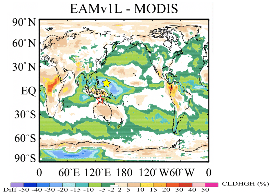
Figure 6Climatological E3SMv1 high cloud bias, computed relative to MODIS observations, from Xie et al. (2018). Open red star shows location of the TWP field campaign, while solid yellow star shows the location we use for our E3SM SCM replay experiment.
We wish to replay a column near the location where the bias is most severe. Therefore we choose a location near 5∘ N and 140∘ E (see yellow star in Fig. 6). The bias in this location is most prevalent during the boreal summer months; therefore we chose August as the month we will replay in SCM mode. In our experimental setup we simply run the GCM with climatologically prescribed SSTs for a year (starting in January) by configuring the simulation with a single directive (“-e3sm_replay”) that will generate the appropriate forcing to replay a column at every E3SM time step. To reduce the amount of output generated, we choose to do a regional subset of the forcing (instructions for this provided at the E3SM SCM wiki). We also chose to output initial condition files at the start of every month so that our SCM can start from the same state as the GCM.
Once the simulation is over we use scripts provided in the E3SM case library to replay our column of choice. The inputs we need to specify are the E3SM-generated forcing file, initial condition file, the latitude and longitude we wish to simulate, and the desired start date and run duration.
Figure 7 displays the monthly mean profiles of cloud fraction, cloud liquid mixing ratio, and cloud ice mixing ratio for the SCM and GCM run for the column of interest. For observations we use CALIPSO, CloudSat, and Moderate Resolution Imaging Spectroradiometer (MODIS) in a merged product called C3M (Kato et al., 2010). The GCM and SCM profiles are averaged over August of the first year of the simulation performed with climatological SSTs, while the C3M data represent the average of August 2006–2010. Figure 7 clearly shows that E3SM underestimates cloud, not only at the upper levels but also the lower and mid levels, by a substantial amount for this column. While the cloud liquid mixing ratio is represented with somewhat reasonable magnitude by the GCM, cloud ice is substantially underpredicted. Thus the combination of the low cloud fraction and cloud ice is likely driving the radiation biases seen in the full GCM for this region.
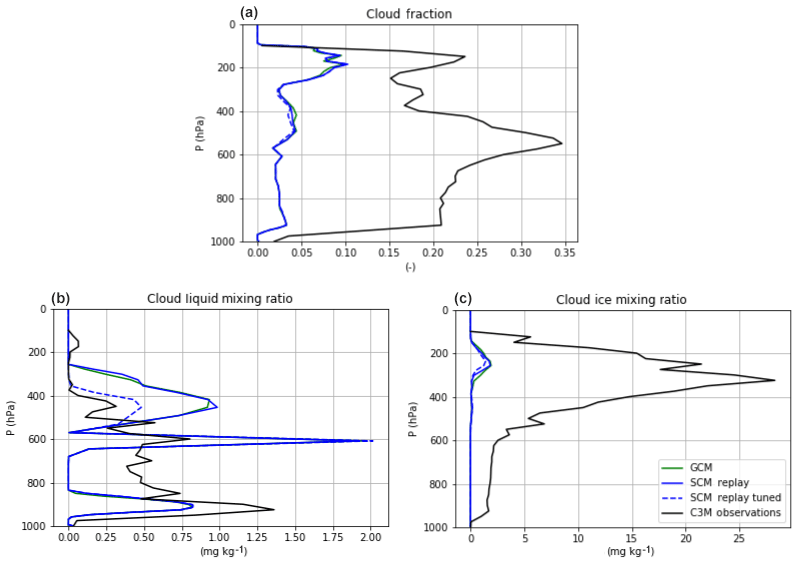
Figure 7Temporally averaged profiles of cloud fraction (a), cloud liquid mixing ratio (b), and cloud ice mixing ratio (c) for C3M observations (black curves), GCM (green curves), and E3SM SCM replay (blue curves) from location 5∘ N and 140∘ E. Profiles from observations represent average over August 2006–2010, while GCM and SCM profiles represent averages from August of a 1-year simulation using prescribed climatological SSTs.
From Fig. 7, it is also clear that the SCM replay mode is also very capable of reproducing the full GCM, as cloud profiles exhibit nearly identical behavior. As a reminder, fully bit-by-bit results are not expected with the E3SM replay mode due to the fact that the dynamics tendency calculation is applied differently than in the full GCM. However, we show here that the replay mode can faithfully represent the behavior of the GCM. While the replay mode cannot provide information on whether the warm pool cloud bias is due to parameterization deficiencies or discrepancies in the large-scale, we can use the SCM replay method to perturb parameterization tunable parameters in an efficient way to explore the effect they might have on the high cloud bias.
As an example of this, we run the SCM in replay mode for this column but with the Bergeron efficiency set to 1.0 (blue dashed curve in Fig. 7), as in Sect. 5.3. In this experiment, while we see noticeable effects in the mid-troposphere in terms of the reduction in cloud liquid, there is little effect towards the increase in cloud fraction or cloud ice mixing ratio. Simultaneously, we also performed several experiments where we perturbed the critical thresholds of the relative humidity for the ice cloud fraction closure (Gettelman et al., 2010), but we saw no noticeable changes in the simulation of the cloud profiles (not shown). While these experiments were not successful towards improving this bias in E3SM, they allowed us to efficiently rule out potential culprits in the tuning choices while avoiding wasting computational resources of testing the same experiments in long climate integrations.
This paper describes the E3SMv1 SCM, including modifications made to it since we adopted it from CAM, and how this configuration can be useful for model development and evaluation. A number of important upgrades were made to E3SM SCM since the inherited version, including the ability for the user to specify how the aerosols are treated to avoid unscientific case setups due to the fact that E3SM initializes all aerosol concentrations to zero. Idealizations have also been implemented and turned on by default, depending on the IOP forcing the user selects, to ensure an apples-to-apples comparison with LES benchmarks that the IOP forcing was meant to replicate. Most importantly, the E3SM SCM is now configured to work with the same dynamical core as the full GCM. This ensures that the SCM runs with the same large-scale vertical advection scheme, time step, and physics–dynamics coupling methods as the full model. It also allows the user to trivially replay a column of the full GCM with the SCM without the need to interpolate initial condition files or forcing files from one dynamical core to the next. The upgrade to the SE dynamical core is also advantageous because E3SM no longer needs to maintain and support the Eulerian dynamical core, which was not used in any other model configuration. We note that the E3SMv1 SCM infrastructure is expected to remain the same for E3SMv2.
The E3SM SCM also has an extensive library of IOP cases that span the traditionally used GCSS boundary layer cloud cases (i.e., BOMEX, DYCOMS, RICO) and standard deep-convection cases (i.e., ARM97, GATE). We also include IOP forcing files from more recent and modern cases, such as GOAMAZON, RACORO, and DYNAMO; many of these are unique to the E3SM SCM. For example, the E3SM can simulate conditions at ARM SGP for 12 continuous years. This allows for robust GCM-like statistics to be generated in a computationally efficient manner. Scripts to run each individual case are available at https://github.com/E3SM-Project/scmlib/wiki/E3SM-Single-Column-Model-Case-Library (last access: 3 March 2020) and many have been scientifically validated. The user need only supply paths to relevant output directories if running on E3SM support machines.
We provide some examples of when the E3SM SCM may prove to be a useful proxy for GCM performance. For instance, we are able to successfully replicate the diurnal cycle of precipitation bias in the GCM by using forcing generated at ARM SGP. This bias is mostly due to deficiencies in the triggering mechanism in the convective parameterization that is unable to properly handle elevated convection. By implementing the trigger improvements documented in XIE2019, we are able to reproduce the same improved diurnal cycle of precipitation in the SCM found in global simulations. However, we were unable to replicate the seasonal cycle of dry Amazon bias with the SCM. We conclude that the root cause of the bias is due to improper representation of the large-scale environment rather than a deficiency with the parameterizations.
Using Arctic clouds as an example, we use the SCM to experiment with tunable parameter changes to evaluate the sensitivity of the high-latitude cloud bias. We report positive effects with the tuning of one parameter for this particular regime, but we caution that the SCM cannot inform how a full GCM simulation and radiation balance would be impacted with a modification. We also compare the SCM in hindcast or free-running mode versus a run where the SCM is nudged to observations. By running in hindcast or free-running mode the SCM allows the model biases in temperature and moisture to naturally develop, thus providing a better proxy with the model behavior in the full GCM; it should therefore be used if trying to replicate E3SM behavior. Nudging the SCM to observations may not provide a proxy with the full GCM and the behavior that could deviate significantly from E3SM global runs. This mode is, however, potentially useful if trying to improve or implement a parameterization while avoiding compensating errors. We caution the user on the potential unintended consequences of adding artificial sources that nudging could introduce.
We also demonstrate that the replay mode in the E3SM SCM can faithfully replicate a column of the GCM, though bit-by-bit replication is not possible in the current implementation. This mode is useful when trying to simulate a particular regime or region that the extensive E3SM case library does not cover. In our example, we replicated the high cloud bias in the Tropical Pacific Warm Pool. While the SCM cannot inform us directly whether biases are caused predominately by deficiencies in the model physics or the large-scale flow, it can provide clues about the culprit. This allows model developers to focus their energies more efficiently on a solution.
The E3SM SCM is mature and should be a first step in the model physics development and implementation process. With the extensive case library and the ability to simulate many different regimes, users can gain valuable insights into their development efforts and efficiently fix bugs. The SCM is also an important tool for addressing long-standing biases in the model; its incredible efficiency makes large sets of perturbed parameter tests easy. In addition, model instabilities that may arise in the full GCM can be investigated efficiently using the easy to use SCM replay mode, which is a powerful tool that can faithfully replicate a column of the full GCM.
The model code used in this study is located at https://doi.org/10.5281/zenodo.3742207 (Bogenschutz, 2020a), while the scripts used to generate the SCM simulations in this paper are located at https://github.com/E3SM-Project/scmlib/wiki/E3SM-Single-Column-Model-Case-Library (last access: 3 March 2020, Bogenschutz, 2020b), and the output from the SCM hindcast simulations can be found at https://portal.nersc.gov/project/mp193/sqtang/E3SM_SCM_runs/ (last access: 17 October 2019, Tang, 2019).
LLNL conceived the study and was the primary developer of the SCM. WL did some of the preliminary development work of the SCM, while YSC provided some crucial code contributions for the replay mode for the SCM. All authors contributed to interpreting the results.
The authors declare that they have no conflict of interest.
This research work was performed under the auspices of the U.S. Department of Energy by LLNL under contract DE-AC52-07NA27344.
This work was part of the CMDV Software Modernization program, funded by the U.S. Department of Energy (DOE) Office of Biological and Environmental Research (grant no. DE-AC52-07NA27344). Yao-Sheng Chen is funded by Scientific Discovery through Advanced Computing (SciDAC) (award no. DE-SC0018650).
This paper was edited by Andrea Stenke and reviewed by two anonymous referees.
Ackerman, A. S., VanZanten, M. C., Stevens, B., Savic-Jovcic, V., Bretherton, C. S., Chlond, A., Golaz, J., Jiang, H., Khairoutdinov, M., Krueger, S. K., Lewellen D. C., Lock A., Moeng C., Nakamura, K., Petters, M. D., Snider, J. R., Weinbrecht, S., and Zulauf, M.: Large-Eddy Simulations of a Drizzling, Stratocumulus-Topped Marine Boundary Layer, Mon. Weather Rev., 137, 1083–1110, https://doi.org/10.1175/2008MWR2582.1, 2009.
Betts, A. K. and Miller, M. J.: A new convective adjustment scheme. Part II: Single column tests using GATE wave, BOMEX, ATEX and arctic air-mass data sets, Q. J. Roy. Meteor. Soc., 112, 693–709, https://doi.org/10.1002/qj.49711247308, 1986.
Bogenschutz, P. A.: The E3SM version 1 Single Column Model code, Zenodo, https://doi.org/10.5281/zenodo.3742207, 2020a.
Bogenschutz, P. A.: E3SM single column case library, available at: https://github.com/E3SM-Project/scmlib/wiki/E3SM-Single-Column-Model-Case-Library, last access: 3 March 2020b.
Bogenschutz, P. A. and Krueger, S. K.: A simplified PDF parameterization of subgrid-scale clouds and turbulence for cloud-resolving models, J. Adv. Model. Earth Sy., 5, 195–211, https://doi.org/10.1002/jame.20018, 2013.
Bogenschutz, P. A., Gettelman, A., Morrison, H., Larson, V. E., Schanen, D. P., Meyer, N. R., and Craig, C.: Unified parameterization of the planetary boundary layer and shallow convection with a higher-order turbulence closure in the Community Atmosphere Model: single-column experiments, Geosci. Model Dev., 5, 1407–1423, https://doi.org/10.5194/gmd-5-1407-2012, 2012.
Bogenschutz, P. A., Gettelman, A., Morrison, H., Larson, V. E., Craig, C., and Schanen, D. P.: Higher-Order Turbulence Closure and Its Impact on Climate Simulations in the Community Atmosphere Model, J. Climate, 26, 9655–9676, https://doi.org/10.1175/JCLI-D-13-00075.1, 2013.
Brown, A. R., Cederwall, R. T., Chlond, A., Duynkerke, P. G., Golaz, J. C., Khairoutdinov, M., Lewellen, D. C., Lock, A. P., MacVean, M. K., Moeng, C.-H., Neggers, R. A. J., Siebesma, A. P., and Stevens, B.: Large-eddy simulation of the diurnal cycle of shallow cumulus convection over land, Q. J. Roy. Meteor. Soc., 128, 1075–1093, https://doi.org/10.1256/003590002320373210, 2002.
Caldwell, P. M., Mametjanov, A., Tang, Q., Van Roekel, L. P., Golaz, J.‐C., Lin, W., Bader, D. C., Keen, N. D., Feng, Y., Jacob, R., Maltrud, M. E., Roberts, A. F., Tayler, M. A., Veneziani, M., Wang, H., Wolfe, J. D., Balaguru, K., Cameron-Smith, P., Dong, L., Klein, S. A., Leung, L., Li, H. Y., Li, Q. L., Liu, X., Neale, R. B., Pinheiro, M., Qian, Y., Ullrich, P. A., Xie, S., Yang, Y., Zhang, Y., Zhang, K., and Zhou, T.: The DOE E3SM coupled model version 1: Description and results at high resolution, J. Adv. Model. Earth Syst., 11, 4095–4146, https://doi.org/10.1029/2019MS001870, 2019.
Covey, C., Gleckler, P. J., Doutriaux, C., Williams, D. N., Dai, A., Fasullo, J., Trenberth, K., and Berg, A.: Metrics for the Diurnal Cycle of Precipitation: Toward Routine Benchmarks for Climate Models, J. Climate, 29, 4461–4471, https://doi.org/10.1175/JCLI-D-15-0664.1, 2016.
Dai, A. and Trenberth K. E.: The Diurnal Cycle and Its Depiction in the Community Climate System Model, J. Climate, 17, 930–951, https://doi.org/10.1175/1520-0442(2004)017<0930:TDCAID>2.0.CO;2, 2004.
Dennis, J. M., Edwards, J., Evans, K. J., Guba, O., Lauritzen, P. H., Mirin, A. A., and Worley, P. H.: CAM-SE: A scalable spectral element dynamical core for the Community Atmosphere Model, Int. J. High Perform. C., 26, 74–89, https://doi.org/10.1177/1094342011428142, 2012.
Gettelman, A., Liu, X., Ghan, S. J., Morrison, H., Park, S., Conley, A. J., Klein, S. A., Boyle, J., Mitchell, D. L., and Li, J.-L. F.:, Global simulations of ice nucleation and ice supersaturation with an improved cloud scheme in the Community Atmosphere Model, J. Geophys. Res., 115, D18216, https://doi.org/10.1029/2009JD013797, 2010.
Gettelman, A., Truesdale, J. E., Bacmeister, J. T., Caldwell, P. M., Neale, R. B., Bogenschutz, P. A., and Simpson, I. R.: The Single Column Atmosphere Model version 6 (SCAM6): Not a scam but a tool for model evaluation and development, J. Adv. Model. Earth Sy., 11, 1381–1401, https://doi.org/10.1029/2018MS001578, 2019.
Ghan, S., Randall, D., Xu, K.-M., Cederwall, R., Cripe, D., Hack, J., Iacobellis, S., Klein, S., Krueger, S., Lohman, U., Pedretti, J., Robock, A., Rotstayn, L., Somerville, R., Stenchikov, G., Sud, Y., Walker, G., Xie, S., Yio, J., and Zhang, M.: A comparison of single column model simulations of summertime midlatitude continental convection, J. Geophys. Res.-Atmos., 105, 2091–2124, https://doi.org/10.1029/1999JD900971, 2000.
Golaz, J., Larson, V. E., and Cotton, W. R.: A PDF-Based Model for Boundary Layer Clouds. Part I: Method and Model Description, J. Atmos. Sci., 59, 3540–3551, https://doi.org/10.1175/1520-0469(2002)059<3540:APBMFB>2.0.CO;2, 2002.
Golaz, J.-C., Caldwell, P. M., Roekel, L. P., Peterson, M. P., Tang, Q., Wolfe, J., Abeshu, G., Anatharaj, V., Asay-Davis, X., Bader, D., Baldwin, S., Bisht, G., Bogenschutz, P., Branstetter, M., Brunke, M., Brus, S., Burrows, S., Cameron-Smith, P., Donahue, A., Deakin, M., Easter, R., Evans, K., Yeng, F., Flanner, M., Foucar, J., Fyke, J., Griffin, B., Hannay, C., Harrop, B., Hoffman, M., Hunke, E., Jacob, R., Jacobsen, D., Jeffery, N., Jones, P., Keen, N., Klein, S., Larson, V., Leung, L., Li, H., Lin, W., Lipscomb, W., Ma, P., Mahajan, S., Maltrud, M., Mametjanov, A., McClean, J., McCoy, R., Neale, R., Price, S., Qian, S., Rasch, P., Eyre, J. E., Riley, W., Ringler, T., Roberts, A., Roesler, E., Salinger, A., Shaheen, Z., Shi, X., Singh, B., Tang, J., Taylor, M., Thorton, P., Turner, A., Veneziani, M., Wan, H., Wang, H., Wang, S., Williams, D., Wolfram, P., Worley, P., Xie, S., Yang, Y., Yoon, J., Zelinka, M., Zender, C., Zeng, X., Zhang, C., Zhang, K., Zhang, Y., Zheng, X., Zhou, T., and Zhu, Q.: The DOE E3SM coupled model version 1: Overview and evaluation at standard resolution, J. Adv. Model. Earth Sy., 11, 2089–2129, https://doi.org/10.1029/2018MS001603, 2019.
Guo, Z., Wang, M., Qian, Y., Larson, V. E., Ghan, S., Ovchinnikov, M., Bogenschutz, P. A., Gettelman, A., and Zhou, T.: Parametric behaviors of CLUBB in simulations of low clouds in the Community Atmosphere Model (CAM), J. Adv. Model. Earth Sy., 7, 1005–1025, https://doi.org/10.1002/2014MS000405, 2015.
Hartung, K., Svensson, G., Struthers, H., Deppenmeier, A.-L., and Hazeleger, W.: An EC-Earth coupled atmosphere–ocean single-column model (AOSCM.v1_EC-Earth3) for studying coupled marine and polar processes, Geosci. Model Dev., 11, 4117–4137, https://doi.org/10.5194/gmd-11-4117-2018, 2018.
Holland, J. Z. and Rasmusson, E. M.: Measurements of the atmospheric mass, energy, and momentum budgets over a 500-kilometer square of tropical ocean, Mon. Weather Rev, 101, 44–55, https://doi.org/10.1175/1520-0493(1973)101<0044:MOTAME>2.3.CO;2, 1973.
Houze, R. A. and Betts, A. K.: Convection in GATE, Rev. Geophys., 19, 541–576, https://doi.org/10.1029/RG019i004p00541, 1981.
Hurrell, J. W., Holland, M. M., Gent, P. R., Ghan, S., Kay, J. E., Kushner, P. J., Lamarque, J., Large, W. G., Lawrence, D., Lindsay, K., Lipscomb, W., Long, M. C., Mahowald, N., Marsh, D. R., Neale, R. B., Rasch, P., Vavrus, S., Vertenstein, M., Bader, D., Collins, W. D., Hack, J. J., Kiehl, J., and Marshall, S.: The Community Earth System Model: A Framework for Collaborative Research, B. Am. Meteorol. Soc., 94, 1339–1360, https://doi.org/10.1175/BAMS-D-12-00121.1, 2013.
Jensen, M. P., Petersen, W. A., Bansemer, A., Bharadwaj, N., Carey, L. D., Cecil, D. J., Collis, S. M., Del Genio, A. D., Dolan, B., Gerlach, J., Giangrande, S. E., Heymsfield, A., Heymsfield, G., Kollias, P., Lang, T. J., Nesbitt, S. W., Neumann, A., Poellot, M., Rutledge, S. A., Schwaller, M., Tokay, A., Williams, C. R., Wolff, D. B., Xie, S., and Zipser, E. J.: The Midlatitude Continental Convective Clouds Experiment (MC3E), B. Am. Meteorol. Soc., 97, 1667–1686, https://doi.org/10.1175/BAMS-D-14-00228.1, 2016.
Kato, S., Sun-Mack, S., Miller, W. F., Rose, F. G., Chen, Y., Minnis, P., and Wielicki, B. A.: Relationships among cloud occurrence frequency, overlap, and effective thickness derived from CALIPSO and CloudSat merged cloud vertical profiles, J. Geophys. Res., 115, D00H28, https://doi.org/10.1029/2009JD012277, 2010.
Klein, S. A., McCoy, R. B., Morrison, H., Ackerman, A. S., Avramov, A., Boer, G. D., Chen, M., Cole, J. N. S., Del Genio, A. D., Falk, M., Foster, M. J., Fridlind, A., Golaz, J. C., Hashino, T., Harrington, J. Y., Hoose, C., Khairoutdinov, M. F., Larson, V. E., Liu, X., Luo, Y., McFarquhar, G. M., Menon, S., Neggers, R. A. J., Park, S., Poellot, M. R., Schmidt, J. M., Sednev, I., Shipway, B. J., Shupe, M. D., Spangenberg, D. A., Sud, Y. C., Turner, D. D., Veron, D.E., Salzen, K. V., Walker, G. K., Wang, Z., Wolf, A. B., Xie, S., Xu, K. M., Yang, F., and Zhang, G.: Intercomparison of model simulations of mixed-phase clouds observed during the ARM Mixed-Phase Arctic Cloud Experiment. I: single-layer cloud, Q. J. Roy. Meteor. Soc., 135, 979–1002, https://doi.org/10.1002/qj.416, 2009.
Lebassi-Habtezion, B. and Caldwell, P. M.: Aerosol specification in single-column Community Atmosphere Model version 5, Geosci. Model Dev., 8, 817–828, https://doi.org/10.5194/gmd-8-817-2015, 2015.
Lee, M.-I., Schubert, S. D., Suarez, M. J., Bell, T. L., and Kim, K.-M.: Diurnal cycle of precipitation in the NASA Seasonal to Interannual Prediction Project atmospheric general circulation model, J. Geophys. Res., 112, D16111, https://doi.org/10.1029/2006JD008346, 2007.
Lee, M.-I., Schubert, S. D., Suarez, M. J., Schemm, J.-K. E., Pan, H.-L., Han, J., and Yoo, S.-H.: Role of convection triggers in the simulation of the diurnal cycle of precipitation over the United States Great Plains in a general circulation model, J. Geophys. Res., 113, D02111, https://doi.org/10.1029/2007JD008984, 2008.
Lin, S.-J. and Rood, R. B.: An explicit flux-form semi-lagrangian shallowwater model on the sphere, Q. J. Roy. Meteor. Soc.,123, 2531–2533, 1997.
Liu, J., Zheng, J., Li, Z., and Cribb, M.: Analysis of cloud condensation nuclei properties at a polluted site in southeastern China during the AMF-China Campaign, J. Geophys. Res.-Atmos., 116, D00K35, https://doi.org/10.1029/2011jd016395, 2011.
Liu, X., Ma, P.-L., Wang, H., Tilmes, S., Singh, B., Easter, R. C., Ghan, S. J., and Rasch, P. J.: Description and evaluation of a new four-mode version of the Modal Aerosol Module (MAM4) within version 5.3 of the Community Atmosphere Model, Geosci. Model Dev., 9, 505–522, https://doi.org/10.5194/gmd-9-505-2016, 2016.
Ma, H.-Y., Chuang, C. C., Klein, S. A., Lo, M.-H., Zhang, Y., Xie, S., Zhang, X., Ma, P.-L., Zhang, Y., and Phillips. T. J.: An improved hindcast approach for evaluation and diagnosis of physical processes in global climate models, J. Adv. Model. Earth Sy., 7, 1810–1827, https://doi.org/10.1002/2015MS000490, 2015.
Mace, J., Jenson, E., McFarquhar, G., Comstock, J. Ackerman, T., Mitchell, D., Liu, X., and Garrett, T.: SPARTICUS: Small particles in cirrus science and operations plans, 33, U.S. Dep. of Energy, Washington, D. C., available at: https://www.arm.gov/publications/programdocs/doe-sc-arm-10-003.pdf (last access: October 2019), 2009.
Martin, S. T., Artaxo, P., Machado, L. A. T., Manzi, A. O., Souza, R. A. F., Schumacher, C., Wang, J., Andreae, M. O., Barbosa, H. M. J., Fan, J., Fisch, G., Goldstein, A. H., Guenther, A., Jimenez, J. L., Pöschl, U., Silva Dias, M. A., Smith, J. N., and Wendisch, M.: Introduction: Observations and Modeling of the Green Ocean Amazon (GoAmazon2014/5), Atmos. Chem. Phys., 16, 4785–4797, https://doi.org/10.5194/acp-16-4785-2016, 2016.
May, P. T., Mather, J. H., Vaughan, G., Jakob, C., McFarquhar, G. M., Bower, K. N., and Mace, G. G.: The Tropical Warm Pool International Cloud Experiment, B. Am. Meteorol. Soc., 89, 629–646, https://doi.org/10.1175/BAMS-89-5-629, 2008.
McFarquhar, G. M., Ghan, S., Verlinde, J., Korolev, A., Strapp, J. W., Schmid, B., Tomlinson, J. M., Wolde, M., Brooks, S. D., Cziczo, D., Dubey, M. K., Fan, J. W., Flynn, C., Gultepe, I., Hubbe, J., Gilles, M. K., Laskin, A., Lawson, P., Leaitch, W. R., Liu P., Liu, X. H., Lubin, D., Mazzoleni, C., Macdonald, A. M., Moffet, R. C., Morrison, H., Ovchinnikov, M., Shupe, M. D., Turner, D. D., Xie, S., Zelenyuk, A., Bae, K., Freer, A., and Glen, A.: Indirect and Semi-direct Aerosol Campaign: The Impact of Arctic Aerosols on Clouds, B. Am. Meteorol. Soc., 92, 183–201, https://doi.org/10.1175/2010bams2935.1, 2011.
Neale, R. B., Chen, C.-C., Gettelman, A., Lauritzen, P. H., Park, S., Williamson D. L., Conley, A. J., Garcia, R., Kinnison, D., Lamarque J.-F., Marsh, D., Mills, M., Smith, A. K., Tilmes, S., Vitt F., Morrison, H., Cameron-Smith, P., Collins, W., Iacono, M. J., Easter, R. C., Ghan, S. J., Liu, X., Rasch, P. J., and Taylor, M. A.: Description of the NCAR Community Atmosphere Model (CAM 5.0), NCAR Technical Note, 289 pp., available at: https://www.cesm.ucar.edu/models/atm-cam/docs/description/description.pdf, last access: November 2012.
Park, S.: A Unified Convection Scheme (UNICON) Part I: Formulation, J. Atmos. Sci., 71, 3902–3930, https://doi.org/10.1175/JAS-D-13-0233.1, 2014.
Randall, D. A. and Cripe, D. G.: Alternative methods for specification of observed forcing in single-column models and cloud system models, J. Geophys. Res.-Atmos., 104, 24527–24545, https://doi.org/10.1029/1999JD900765, 1999.
Randall, D. A., Xu, K., Somerville, R. J., and Iacobellis, S.: Single-Column Models and Cloud Ensemble Models as Links between Observations and Climate Models, J. Climate, 9, 1683–1697, https://doi.org/10.1175/1520-0442(1996)009<1683:SCMACE>2.0.CO;2, 1996.
Rasch, P. J., Xie, S., Ma, P.-L., Lin, W., Wang, H., Tang, Q., Burrows, S., Caldwell, P., Zhang, K., Easter, R., Cameron-Smith, P., Singh, B., Wan, H., Golaz, J.-C., Harrop, B., Roesler, E., Bacmeister, J., Larson, V., Evans, K., Qian, Y., Taylor, M., Leung, L., Zhang, Y., Brent, L., Branstetter, M., Hannay, C., Mahajan S., Mametjanov, A., Neale, R., Richter, J., Yoon, J-H., Zender, C., Bader, B., Flanner, D., Flanner, M., Foucar, J., Jacob, R., Keen, N., Klein, S., Liu, X., Salinger, A., Shrivastava, M., and Yang, Y.: An Overview of the Atmospheric Component of the Energy Exascale Earth System Model, J. Adv. Model. Earth Sy., 11, 2377–2411, https://doi.org/10.1029/2019MS001629, 2019.
Rauber, R. M., Stevens, B., Ochs, H. T., Knight, C., Albrecht, B. A., Blyth, A. M., Fairall, C. W., Jensen, J. B., Lasher-Trapp, S. G., Mayol-Bracero, O. L., Vali, G., Anderson, J. R., Baker, B. A., Bandy, A. R., Burnet, E., Brenguier, J., Brewer, W. A., Brown, P. R., Chuang, R., Cotton, W. R., Di Girolamo, L., Geerts, B., Gerber, H., Goke, S., Gomes, L., Heikes, B. G., Hudson, J. G., Kollias, P., Lawson, R. R., Krueger, S. K., Lenschow, D. H., Nuijens, L., O'Sullivan, D. W., Rilling, R. A., Rogers, D. C., Siebesma, A. P., Snodgrass, E., Stith, J. L., Thornton, D. C., Tucker, S., Twohy, C. H., and Zuidema, P.: Rain in Shallow Cumulus Over the Ocean: The RICO Campaign, B. Am. Meteorol. Soc., 88, 1912–1928, https://doi.org/10.1175/BAMS-88-12-1912, 2007.
Schubert, W. H., Wakefield, J. S., Steiner, E. J., and Cox, S. K.: Marine Stratocumulus Convection. Part I: Governing Equations and Horizontally Homogeneous Solutions, J. Atmos. Sci., 36, 1286–1307, https://doi.org/10.1175/1520-0469(1979)036<1286:MSCPIG>2.0.CO;2, 1979.
Siebesma, A. P., Bretherton, C. S., Brown, A., Chlond, A., Cuxart, J., Duynkerke, P. G., Jiang, H., Khairoutdinov, M., Lewellen, D., Moeng, C.-H., Sanchez E., Stevens, B., and Stevens, D. E.: A Large Eddy Simulation Intercomparison Study of Shallow Cumulus Convection, J. Atmos. Sci., 60, 1201–1219, https://doi.org/10.1175/1520-0469(2003)60<1201:ALESIS>2.0.CO;2, 2003.
Smalley, M., Suselj, K., Lebsock, M., and Teixeira, J.: A novel framework for evaluating and improving parameterized subtropical marine boundary layer clouds, Mon. Weather Rev., 147, 3241–3260, https://doi.org/10.1175/MWR-D-18-0394.1, 2019.
Stevens, B., Ackerman, A. S., Albrecht, B. A., Brown, A. R., Chlond, A., Cuxart, J., Duynkerke, P. G., Lewellen, D. C., Macvean, M. K., Neggers, R. A., Sanchez, E., Siebesma, A. P., and Stevens, D. E.: Simulations of Trade Wind Cumuli under a Strong Inversion, J. Atmos. Sci., 58, 1870–1891, https://doi.org/10.1175/1520-0469(2001)058<1870:SOTWCU>2.0.CO;2, 2001.
Stevens, B., Moeng, C.-H., Ackerman, A. S., Bretherton, C. S., Chlond, A., De Roode, S., Edwards, J., Golaz, J.-C., Jiang, H., Khairoutdinov, M., Kirkpatrick, M. P., Lewellen, D. C., Lock, A., Muller, F., Stevens, D. E., Whelan, E., and Zhu, P.: Evaluation of Large-Eddy Simulations via Observations of Nocturnal Marine Stratocumulus, Mon. Weather Rev., 133, 1443–1462, https://doi.org/10.1175/MWR2930.1, 2005.
Suselj, K., Teixeira, J., and Chung, D.: A Unified Model for Moist Convective Boundary Layers Based on a Stochastic Eddy-Diffusivity/Mass-Flux Parameterization, J. Atmos. Sci., 70, 1929?1953, https://doi.org/10.1175/JAS-D-12-0106.1, 2013.
Tang, S.: E3SM single column model case output, available at: https://portal.nersc.gov/project/mp193/sqtang/E3SM_SCM_runs/, last access: 17 October 2019.
Tang, S., Xie, S., Zhang, Y., Zhang, M., Schumacher, C., Upton, H., Jensen, M. P., Johnson, K. L., Wang, M., Ahlgrimm, M., Feng, Z., Minnis, P., and Thieman, M.: Large-scale vertical velocity, diabatic heating and drying profiles associated with seasonal and diurnal variations of convective systems observed in the GoAmazon2014/5 experiment, Atmos. Chem. Phys., 16, 14249–14264, https://doi.org/10.5194/acp-16-14249-2016, 2016.
Tang, S., Xie, S., Zhang, M., Tang, Q., Zhang, Y., Klein, S. A., Cook, D., and Sullivan, R. C.: Differences in Eddy-Correlation and Energy-Balance Surface Turbulent Heat Flux Measurements and Their Impacts on the Large-Scale Forcing Fields at the ARM SGP Site, J. Geophys. Res.-Atmos., 124, 3301–3318, https://doi.org/10.1029/2018JD029689, 2019.
Verlinde, J., Harrington, J. Y., McFarquhar, G. M., Yannuzzi, V. T., Avramov, A., Greenberg, S., Johnson, N., Zhang, G., Poellot, M. R., Mather, J. H., Turner, D. D., Eloranta, E. W., Zak, B. D., Prenni, A. J., Daniel, J. S., Kok, G. L., Tobin, D. C., Holz, R., Sassen, K., Spangenberg, D., Minnis, P., Tooman, T. P., Ivey, M. D., Richardson, S. J., Bahrmann, C. P., Shupe, M., DeMott, P. J., Heymsfield, A. J., and Schofield, R.: The Mixed-Phase Arctic Cloud Experiment, B. Am. Meteorol. Soc., 88, 205–222, https://doi.org/10.1175/BAMS-88-2-205, 2007.
Vogelmann, A. M., McFarquhar, G. M., Ogren, J. A., Turner, D. D., Comstock, J. M., Feingold, G., Long, C. N., Jonsson, H. H., Bucholtz, A., Collins, D. R., Diskin, G. S., Gerber, H., Lawson, R. P., Woods, R. K., Andrews, E., Yang, H., Chiu, J. C., Hartsock, D., Hubbe, J. M., Lo, C., Marshak, A., Monroe, J. W., McFarlane, S. A., Schmid, B., Tomlinson, J. M., and Toto, T.: RACORO Extended-Term Aircraft Observations of Boundary Layer Clouds, B. Am. Meteorol. Soc., 93, 861–878, https://doi.org/10.1175/BAMS-D-11-00189.1, 2012.
Webster, P. J. and Lukas, R.: TOGA COARE: The Coupled Ocean-Atmosphere Response Experiment, B. Am. Meteorol. Soc., 73, 1377–1416, https://doi.org/10.1175/1520-0477(1992)073<1377:TCTCOR>2.0.CO;2, 1992.
Xie, S., Xu, K.-M., Cederwall, R. T., Bechtold, P., Genio, A. D., Klein, S. A., Cripe, D., Ghan, S. J., David, G., Iacobellis, S. F., Krueger, S. K., Lohmann, U., Petch, J. C., Randall, D. A., Rotstayn, L. D., Sommerville, C. J., Yogesh, C., Salzen, K., Walker, G. K., Wolf, A., Yio, J. J., Zhang, G., and Zhang, M.: Intercomparison and Evaluation of Cumulus Parameterization under Summertime Midlatitude Continental Conditions, Q. J. Roy. Meteor. Soc., 128, 1095–1136, 2002.
Xie, S., Cederwall, R. T., and Zhang, M.: Developing long-term single-column model/cloud system-resolving model forcing data using numerical weather prediction products constrained by surface and top of the atmosphere observations, J. Geophys. Res., 109, D01104, https://doi.org/10.1029/2003JD004045, 2004.
Xie, S., Klein, S., Zhang, M., Yio, J., Cederall, R., and McCoy, R.: Developing large-scale forcing data for single-column and cloud-resolving models from the Mixed-Phase Arctic Cloud Experiment, J. Geophys. Res., 111, D19104, https://doi.org/10.1029/2005JD006950, 2006.
Xie, S., Hume, T., Jakob, C., Klein, S., McCoy, R., and Zhang, M.: Observed large-scale structures and diabatic heating and drying profiles during TWP-ICE, J. Climate, 23, 57–79, https://doi.org/10.1175/2009JCLI3071.1, 2010.
Xie, S., Zhang, Y., Giangrande, S. E., Jensen, M. P., McCoy, R., and Zhang, M.: Interactions between cumulus convection and its environment as revealed by the MC3E sounding array, J. Geophys. Res.-Atmos., 119, 11784–11808, https://doi.org/10.1002/2014JD022011, 2014.
Xie, S., Lin, W., Rasch, P. J., Ma, P.-L., Neale, R., Larson, V. E., et al.: Understanding cloud and convective characteristics in version 1 of the E3SM atmosphere model, J. Adv. Model. Earth Syst., 10, 2618-2644. https://doi.org/10.1029/2018MS001350, 2018.
Xie, S., Wang, Y.-C., Lin, W., Ma, H.-Y., Tang, Q., Tang, S., Zheng, X., Golaz, J.-C., Zhang, G. J., and Zhang, M.: Improved diurnal cycle of precipitation in E3SM with a revised convective triggering function, J. Adv. Model. Earth Sy., 11, 2290–2310, https://doi.org/10.1029/2019MS001702, 2019.
Yoneyama, K., Zhang, C., and Long, C. N.: Tracking Pulses of the Madden-Julian Oscillation, B. Am. Meteorol. Soc., 94, 1871–1891, https://doi.org/10.1175/BAMS-D-12-00157.1, 2013.
Zhang, K., Wan, H., Liu, X., Ghan, S. J., Kooperman, G. J., Ma, P.-L., Rasch, P. J., Neubauer, D., and Lohmann, U.: Technical Note: On the use of nudging for aerosol–climate model intercomparison studies, Atmos. Chem. Phys., 14, 8631–8645, https://doi.org/10.5194/acp-14-8631-2014, 2014.
Zhang, M. and Bretherton, C.: Mechanisms of Low Cloud-Climate Feedback in Idealized Single-Column Simulations with the Community Atmospheric Model, Version 3 (CAM3), J. Climate, 21, 4859–4878, https://doi.org/10.1175/2008JCLI2237.1, 2008.
Zhang, M. H. and Lin, J. N.: Constrained Variational Analysis of Sounding Data Based on Column-Integrated Budgets of Mass, Heat, Moisture, and Momentum: Approach and Application to ARM Measurements, J. Atmos. Sci., 54, 1503–1524, https://doi.org/10.1175/1520-0469(1997)054<1503:CVAOSD>2.0.CO;2, 1997.
Zhang, Y., Xie, S., Lin, W., Klein, S. A., Zelinka, M., Ma, P.‐L., Rasch, P. J., Qian, Y., Tang, Qi., and Ma, H.-Y: Evaluation of clouds in version 1 of the E3SM atmosphere model with satellite simulators, J. Adv. Model. Earth Sy., 11, 1253–1268, https://doi.org/10.1029/2018MS001562, 2019.
Zheng, X., Klein, S. A., Ma, H.-Y., Caldwell, P., Larson, V. E., Gettelman, A., and Bogenschutz, P.: A cloudy planetary boundary layer oscillation arising from the coupling of turbulence with precipitation in climate simulations, J. Adv. Model. Earth Sy., 9, 1973–1993, https://doi.org/10.1002/2017MS000993, 2017.