On the increased climate sensitivity in the EC-Earth model from CMIP5 to CMIP6

Many modelling groups that contribute to CMIP6 (Coupled Model Intercomparison Project Phase 6) have found a larger equilibrium climate sensitivity (ECS) with their latest model versions compared with the values obtained with the earlier versions used in CMIP5. This is also the case for the EC-Earth model. Therefore, in this study, we investigate what developments since the CMIP5 era could have caused the increase in the ECS in this model. Apart from increases in the horizontal and vertical resolution, the EC-Earth model has also substantially changed the representation of aerosols; in particular, it has introduced a more sophisticated description of aerosol indirect effects. After testing the model with some of the recent updates switched off, we find that the ECS increase can be attributed to the more advanced treatment of aerosols, with the largest contribution coming from the effect of aerosols on cloud microphysics (cloud lifetime or second indirect effect). The increase in climate sensitivity is unrelated to model tuning, as all experiments were performed with the same tuning parameters and only the representation of the aerosol effects was changed. These results cannot be generalised to other models, as their CMIP5 and CMIP6 versions may differ with respect to aspects other than the aerosol–cloud interaction, but the results highlight the strong sensitivity of ECS to the details of the aerosol forcing.

1 Introduction

The equilibrium climate sensitivity (ECS) is the average change in the global and annual mean near-surface air temperature (T2m) following an instantaneous doubling of the CO₂ concentration compared with pre-industrial levels, after the climate has reached a new equilibrium. It is a widely used metric in climate modelling to illustrate the warming from increased CO₂ levels including feedbacks in the climate system. The ECS is also highly relevant for climate policy: Matthews et al. (2009) found that global warming mainly depends on the total cumulative anthropogenic emission of carbon to the atmosphere and that the details of the emission pathways are of secondary importance for the warming. The larger the ECS, the smaller the amount of carbon that still can be emitted in order to limit the warming to a value below a given level, e.g. warming levels suggested by the Paris Agreement.

Despite the simple definition of the ECS, it is not easy to constrain its value with observations or models (Roe and Armour, 2011; Knutti et al., 2017). The majority of CMIP5 models have an ECS in the range between 2.1 and 4.7 K (IPCC, 2013). As the first results from CMIP6 models have become accessible, it has been found that the ECS has increased substantially for a number of models compared with the values that were found for CMIP5 (Zelinka et al., 2020) using the predecessors of the very same models (e.g. Mauritsen et al., 2019; Gettelman et al., 2019; Valdoire et al., 2019); this has already led to discussions about the possible implications of higher climate sensitivity (Voosen, 2019, https://www.carbonbrief.org/guest-post-why-results-from-the-next-generation-of-climate-models-matter last access: 28 July 2020). Our EC-Earth model also shows an increased sensitivity: EC-Earth2 (hereafter ECE2), which was used for CMIP5, had an ECS of 3.3 K that has increased to 4.3 K in the newer model version EC-Earth3 (hereafter ECE3) that is used for CMIP6. The goal of this study is to identify and quantify the contributions of model updates when going from ECE2 to ECE3. Unfortunately, the complex nature of the model development process makes it impossible to turn back the development steps using a systematic and continuous approach. Some of the newly introduced processes or forcing datasets can only be switched on or off in combination with others; for example, the more advanced treatment of aerosol indirect effects can only be used in combination with the new aerosol representation in ECE3 that has no equivalent in ECE2. Nevertheless, we attempt to analyse the reasons for the ECS increase using systematic model sensitivity experiments to test the contributions from the various steps during the model developments.

The goal of this study is not to justify the higher ECS of ECE3 nor that of CMIP6 models in general; we only aim to investigate possible reasons for the increase in the ECS in the EC-Earth model family when advancing from the CMIP5 to the CMIP6 version of the model. General constraints on the ECS are outside the scope of this study as are general findings on the ECS for all CMIP6 models, which have been addressed elsewhere (Zelinka et al., 2020; Flynn and Mauritsen, 2020). Any conclusion presented here is valid only for the ECE3 model; however, as many climate models share model components and/or forcings, the findings presented here could also hint at possible reasons for a higher ECS in other models.

2 Method

2.1 The EC-Earth model

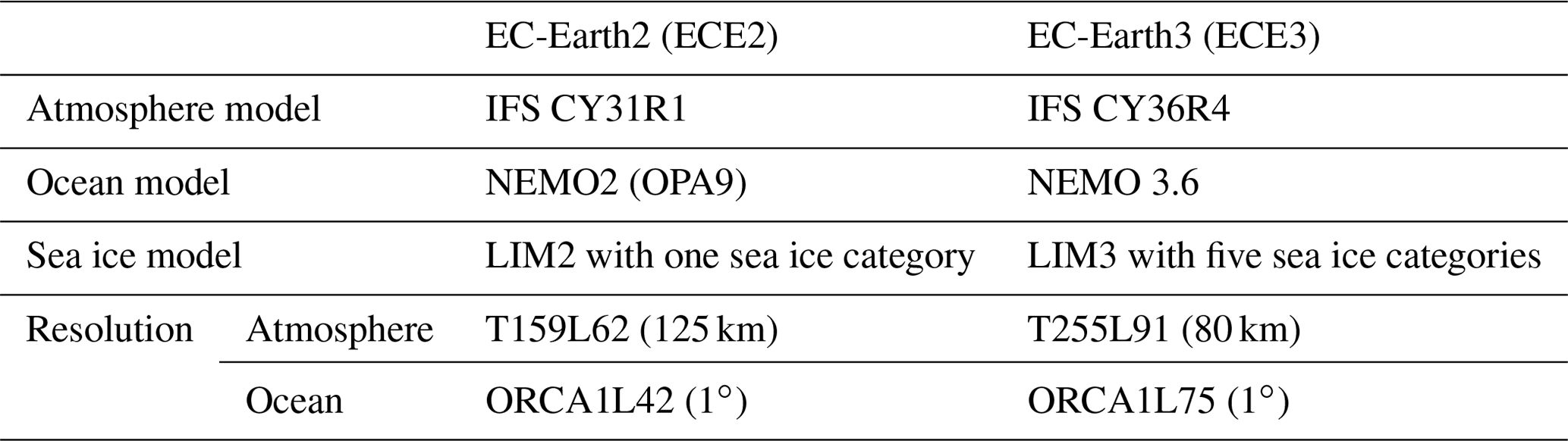
The CMIP5 version of the EC-Earth model is based on CY31R1 from the Integrated Forecasting System (IFS) of the European Centre for Medium-Range Weather Forecasts (ECMWF) and the NEMO version 2 ocean model (OPA9 with the LIM2 sea ice model), see Hazeleger et al. (2012) for details. All components have been upgraded for the new ECE3 model that is used for CMIP6. A detailed description of ECE3 is in preparation (Döscher et al., 2020). The differences in the model components and resolutions between ECE2 and ECE3 are listed in Table 1. In addition to the differences between the model versions, there are also differences in the forcing datasets when going from CMIP5 to CMIP6, e.g. the greenhouse gases (GHGs, Meinshausen et al., 2019) or the aerosol forcing datasets (Stevens et al., 2017), but the impact of the changes in the external forcing on the ECS is outside the scope of this study.

Table 1 CMIP5 and CMIP6 versions of the EC-Earth model family.

The ECE3 model is used to contribute to CMIP6 in several configurations. For the work here, we used the EC-Earth3-Veg configuration which couples the LPJ-Guess dynamic vegetation model (Smith et al., 2014) to the atmosphere and ocean model; however, the performance of EC-Earth3 and EC-Earth3-Veg is very similar.

A noteworthy difference between ECE2 and ECE3 is the way that the aerosols are treated. In EC-Earth2, aerosols are prescribed as mass concentration fields following the CMIP5 time series from the Community Atmosphere Model (CAM; Lamarque et al., 2011). The provided aerosol components are mapped onto the aerosol types used in the IFS and fed into the short- and longwave radiation scheme (direct effect). The cloud effective radius r_eff is computed by distributing the cloud water on a fixed number of droplets following Martin et al. (1994):

$$\begin{array}{}\text{(1)}& r_{\text{eff}}={\left({\displaystyle \frac{\mathrm{3}L}{\mathrm{4}\mathit{\pi }k{N}_{\text{d}}}}\right)}^{\mathrm{1}/\mathrm{3}},\end{array}$$

Here, L is the liquid water content, N_d is the number of droplets and k is a proportionality factor derived from observations. Both N_d and k have fixed values over land and over sea: over land N=313.2 and k=0.688, and over sea N=50.6 and k=0.775. The number of droplets is independent of the CMIP5 aerosol data. Hence, ECE2 only accounts for the direct radiative effects of the prescribed changes in aerosol concentrations in the forcing dataset, but it has no representation of the indirect effects via the aerosol impact on clouds.

ECE3 includes a representation of the direct and indirect aerosol effects. For the direct aerosol effects in the shortwave, the model uses the optical properties of the aerosol plumes provided by the MACv2-SP simple plume model (Stevens et al., 2017) in combination with monthly climatologies of the optical properties of the pre-industrial background aerosol concentration; the latter were obtained from an off-line simulation using the TM5 atmospheric composition model (Van Noije et al., 2014; Bergman et al., 2020) forced with pre-industrial emissions for CMIP6 (Hoesly et al., 2018; Van Marle et al., 2017). The aerosol effects in the longwave are calculated based on the background aerosol mass concentrations obtained from the pre-industrial TM5 simulation. For the indirect aerosol effect, the number of activated aerosols is computed following the work of Abdul-Razzak and Ghan (2000). The Abdul-Razzak and Ghan (2000) scheme parameterises the number of activated aerosols of multiple externally mixed lognormal aerosol modes, each composed of a uniform internal mixture of soluble and insoluble material. The Köhler theory is used to relate the aerosol size distribution and composition to the number activated as a function of maximum supersaturation. The supersaturation balance is used to determine the maximum supersaturation, accounting for particle growth both before and after the particles are activated.

Indirect aerosol effects are accounted for by making the effective radius and autoconversion efficiency depend on the concentration of cloud droplets (CDNC). The effective radius is still computed as shown in Eq. (1), but the constant droplet concentration N_d is replaced by the dynamic CDNC. The autoconversion efficiency a is a linear function of cloud water above a given threshold following Sundqvist (1978):

$$\begin{array}{}\text{(2)}& a=c_{\mathrm{0}}\left(\mathrm{1}-e^{-{\left(\frac{L}{L_{\text{crit}}}\right)}^{\mathrm{2}}}\right),\end{array}$$

where $c_{\mathrm{0}}^{-\mathrm{1}}$ represents a characteristic timescale for the conversion of cloud liquid droplets, L is the liquid water content and L_crit is the typical cloud water content at which the generation of precipitation begins to be efficient. To account for the variation in the cloud droplet number through aerosol activation, the autoconversion efficiency is scaled with the CDNC following Rotstayn and Penner (2001):

$$\begin{array}{}\text{(3)}& a^{\prime }=a{\left({\displaystyle \frac{N_{\mathrm{0}}}{N}}\right)}^{\mathrm{1}/\mathrm{3}},\end{array}$$

with N₀=125 cm⁻¹ and N= CDNC the actual cloud condensation nuclei concentration.

The aerosol number and mass concentration fields that serve as input to the activation scheme are climatologies from the off-line pre-industrial run with TM5. The changes in aerosol concentrations since the pre-industrial era in transient simulations for CMIP6 are accounted for by multiplying the resulting cloud droplet number concentration by the multiplication factor provided by MACv2-SP. Note, however, that the pre-industrial aerosol concentrations are used without any multiplication factor in the pre-industrial control experiment (piControl) and abrupt-4xCO2 (hereafter referred to as 4xCO2) experiments for this study, following the experimental protocol for these CMIP6 experiments.

2.2 Experiment design

ECS is assessed by comparing the response of the net top-of-the-atmosphere (TOA) radiative flux (Q_net) and T2m from the 4xCO2 experiment against the piControl experiment with its baseline CO₂ concentration. Therefore, each model modification requires two long model simulations: one with the baseline and one with a quadrupled CO₂ concentration. In a first step, we compare ECS between the CMIP5 and CMIP6 versions of the EC-Earth model. We then analyse changes in the global means and in the regional distribution of clouds and their impact on the cloud forcing (CF; the difference between all-sky and clear-sky net radiation) to investigate the difference in climate sensitivity between ECE2 and ECE3.

To better understand the role of the various improvements during the development process of ECE3, we roll back some of the changes and measure the impact on the CF and ECS in a series of sensitivity experiments. Apart from the changes in model resolution, the most relevant updates of the model are those related to the revised treatment of the aerosols and their interaction with clouds. The question is if and possibly how much any of these changes have contributed to the increase in ECS that we find when comparing the CMIP5 and the CMIP6 versions of the EC-Earth model.

The CMIP6 protocol requires the 4xCO2 experiments to be 150 years long; however, in order to save computational resources, we test if 75-year-long sensitivity experiments could give an acceptable estimate of the ECS. In another attempt to save computational resources, we investigate if the ECS depends on the model resolution. The horizontal and vertical resolution of the atmosphere model in ECE3 is reduced to the resolution that was used for CMIP5. A reduction in the simulation length and the lower resolution allows us to perform more experiments with the available computational resources; however, we first need to establish that these modifications only have a small impact on the ECS of the model.

2.3 Assessing the equilibrium climate sensitivity

ECS is defined as the increase in the global mean T2m between a steady-state climate with pre-industrial levels of CO₂ concentrations and the steady-state climate with doubled CO₂ concentrations, with all other forcings (e.g. GHGs, aerosols and land use) remaining at pre-industrial conditions. Despite this simple and straightforward definition of the ECS, the practical task of assessing the ECS of a model is a real challenge because requires the model to run with an increased CO₂ concentration until it reaches equilibrium. However, the brute force approach to run the model until equilibrium is not very practical, as it would take thousands of years of model integration to bring the deep ocean into equilibrium and to find the steady-state equilibrium temperature (e.g. Stouffer, 2004; Paynter et al., 2018; Rugenstein et al., 2020). For this reason, modellers often apply the method proposed by Gregory et al. (2004) that has also been used to estimate ECS in CMIP5 (IPCC 2013, Andrews et al., 2012) and CMIP6 models (e.g. Andrews et al., 2019; Voldoire et al., 2019; Zelinka et al., 2020). Here, we apply the Gregory method to the 4xCO2 experiments for CMIP6 which are only 150 years long (Eyring et al., 2016). When running a simulation with increased CO₂ concentrations, the global mean Q_net and T2m asymptotically approach the equilibrium state; thus, by extrapolating a linear fit of the data points to the Q_net=0 level, one can obtain an estimate of the equilibrium temperature that would be reached when the model reaches its new equilibrium, which is characterised by a zero TOA energy balance. Apart from the ECS, the Gregory method allows one to estimate two other important model parameters: the intercept of the linear fit with the ordinate, which indicates the effective radiative forcing (ERF) for a quadrupling of the CO₂ concentration, and the slope of the linear regression, which is known as the radiative feedback parameter (λ) and expresses the strength of the feedback. As models may present an energy balance that is not perfectly closed, resulting in a nonzero equilibrium TOA net flux, the pre-industrial equilibrium values are typically removed from the 4xCO2 values before proceeding with the fit to determine the ECS.

By definition, the ECS is the temperature change that results from a doubling of the CO₂ concentrations. However, the DECK (Diagnostic, Evaluation and Characterization of Klima) experiments for CMIP6 comprise the abrupt-4xCO2 experiment with instantaneously quadrupled CO₂ (Eyring et al., 2016). Following common practice (e.g. Andrews et al., 2012; IPCC, 2013, Knutti et al., 2017; Zelinka et al., 2020), we divide the estimate for the equilibrium temperature and effective radiative forcing in the 4xCO2 experiment by 2 to obtain estimates of the ECS and ERF for a doubling of the CO2 concentration.

Correction for model drift

With a steady-state control climate in the piControl experiment, it is straightforward to evaluate the TOA radiation imbalance and temperature response at the surface in a sensitivity experiment with changed forcing relative to the control climate. The control climate and response to changed forcing are evaluated in corresponding time periods in the control and sensitivity experiment respectively. However, when testing the sensitivity of the ECS to recent model changes we switch some model features on and off which may result in an ill-tuned model and introduce a drift. In principle, one would have to first make a new spin-up run with the modified model before starting new piControl and 4xCO2 experiments; however, limited computational resources prohibit us from carrying out several long spin-up runs with slightly modified model configurations. To overcome this difficulty, we assume that the model modifications only lead to a small drift in the pre-industrial control climate that we can correct for. After carrying out the experiment with pre-industrial forcing with each model modification, we first make linear fits of the Q_net and T2m time series and then use these regressions to correct the time series of the corresponding 4xCO2 experiment (Fig. 1), following common practice (e.g. Andrews et al., 2015). We also apply a similar correction to the unperturbed control experiment. As the largest shock caused by a model modification occurs right at the start of the simulation and may give rise to a non-linear response, we exclude the first five annual means when computing the linear fit for the model drift. For the same reason, we also exclude the first 5 years of the net radiation and temperature time series when computing the linear regression for estimating the ECS. We have tested the impact on the ECS when excluding a few years from the dataset, and we find that the result no longer changes if 4 or more years are excluded. We have verified that the resulting ECS estimates are very close to the values obtained with more advanced linear regression methods that are more robust against outliers (e.g. Theil–Sen regression), confirming that the strongest deviations from the linear relation are indeed observed during the first few years.

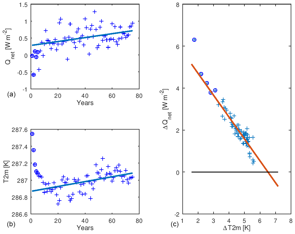
Figure 1 Time series of Q_net (a) and T2m (b) in a pre-industrial simulation with CMIP5 aerosols and without explicit cloud droplet activation. The model is not tuned for this configuration and, therefore, experiences a drift over time. The linear regression (solid) in the Q_net and T2m plot provides the offset and drift correction that are later subtracted from the 4xCO2 experiment with the same model configuration. The first 5 years (marked using circles in the plot) are excluded when computing the linear fit. (c) A Gregory plot from the 4xCO2 experiment for the same model configuration after correcting for offset and drift in the corresponding experiment with pre-industrial forcing. A regression line is fitted to the data points (red) and extrapolated, again excluding the first 5 years (marked using circles in the plot). The intersection of this line with the ΔQ_net=0 line is an estimate of the equilibrium temperature response in the 4xCO2 experiment. This value has to be divided by 2 to yield an estimate for the equilibrium climate sensitivity (ECS).

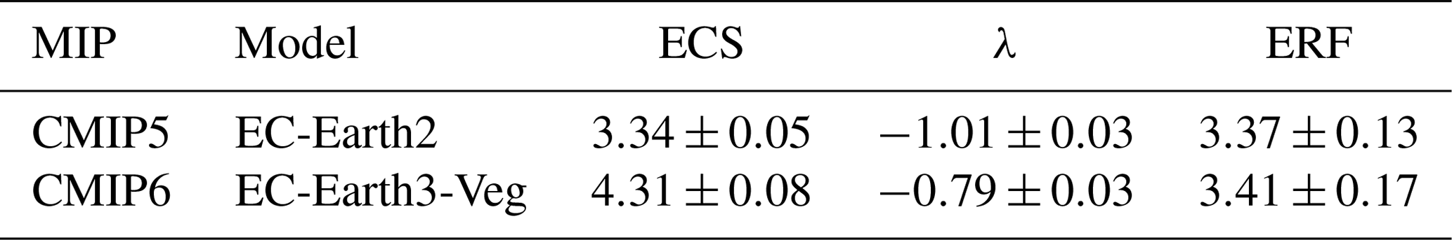
Table 2 Equilibrium climate sensitivity (ECS, in K), net feedback parameter (λ, in W m⁻² K⁻¹) and effective radiative forcing (ERF, in W m⁻²) in the CMIP5 and CMIP6 versions of the EC-Earth model.

3 Results

3.1 Climate sensitivity in ECE2 and ECE3

Table 2 presents the ECS, the net feedback and the ERF for the CMIP5 and CMIP6 versions of the EC-Earth model. ECS increases from 3.34 to 4.31 K. Zelinka et al. (2020) conclude that the higher ECS of many CMIP6 models is due to a combination of a higher ERF and a weaker net feedback compared with the model versions that have been used for CMIP5. However, the EC-Earth model is slightly different from other models because its ERF does not change much between the CMIP5 and CMIP6 versions; therefore, the different ECS in ECE2 and ECE3 is mainly caused by a different net feedback parameter. The small change in the ERF from ECE2 to ECE3 can explain the comparably weak increase in ECS in the EC-Earth model, while other models show considerably larger increase between their CMIP5 and CMIP6 versions, although Zelinka et al. (2020) conclude that the differences are not significant.

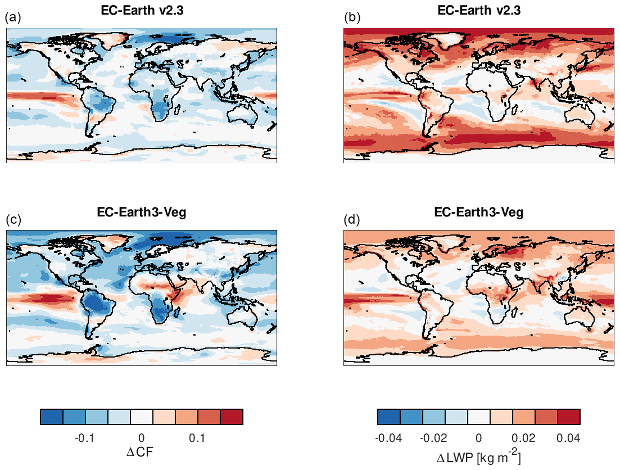
Figure 2 Response of cloud fraction (a, c) and the cloud liquid water path (LWP) (b, d) to a quadrupling of CO₂ in ECE2 (a, b) and ECE3 (c, d).

Figure 3 Same as Fig. 2 but for net cloud forcing.

To analyse the causes of the change in the net feedback parameter, one must look at the response in the 4xCO2 experiments in ECE2 and ECE3. Figure 2 shows the change in clouds at the end (years 131 to 150) of the 4xCO2 experiment relative to the piControl experiment. We find different behaviour in the different versions of the model: ECE2 shows a weaker response in the cloud cover than ECE3, in particular over North Hemisphere Atlantic and Pacific oceans, whereas ECE2 shows a stronger response in the cloud liquid water path (LWP) in the extratropics. The response of the vertically integrated cloud ice has a similar pattern in ECE2 and ECE3 but is somewhat stronger in ECE3 (not shown). These differences in the response of the cloud fraction and the LWP due to a quadrupling of CO2 also have an impact on the cloud forcing (CF; Fig. 3). In ECE2 the response in the CF is weak except at high latitudes, which results from the melting of sea ice in a warmer climate. In contrast, ECE3 shows a more pronounced response in the cloud forcing. In the tropics, CF becomes more negative, whereas the response is positive over the Northern Hemisphere Atlantic and Pacific oceans, leading to a less negative cloud forcing.

These changes in the response of clouds and, subsequently, cloud forcing can explain the change in the climate sensitivity of the EC-Earth model between the CMIP5 and the CMIP6 versions. The question is then what modifications of the cloud parameterisation during the development of ECE3 play an important role in the changes in the response to an increased CO2 forcing, and what impact these model updates have on the ECS. To study the effects of different model development steps, we roll back the developments that are related to the aerosol and cloud interaction, and then we repeat the piControl and abrupt-4xCO2 experiments in a series of sensitivity studies.

3.2 Reducing the length of the simulation

Reducing the length of the piControl and 4xCO2 simulations would make the sensitivity experiments computationally cheaper, but it could only be done if the impact on the ECS is small. In order to test this, we compute the ECS from our DECK experiments (EC-Earth Consortium, 2019a, b) by taking 150 and 75 years of the annual mean time series respectively. In both cases the model configuration is EC-Earth3-Veg with the full T255L91–ORCA1L75 resolution used for CMIP6. The ECS is found not to be significantly different irrespective of whether 150 or 75 years are included in the linear regression (Table 2). Therefore, we conclude that we can safely reduce the length of the sensitivity experiments with minimal impact on the ECS.

Table 3 Impact of a reduced simulation length and reduced model resolution on the ECS. The ECS value for EC-Earth2 is shown for comparison.

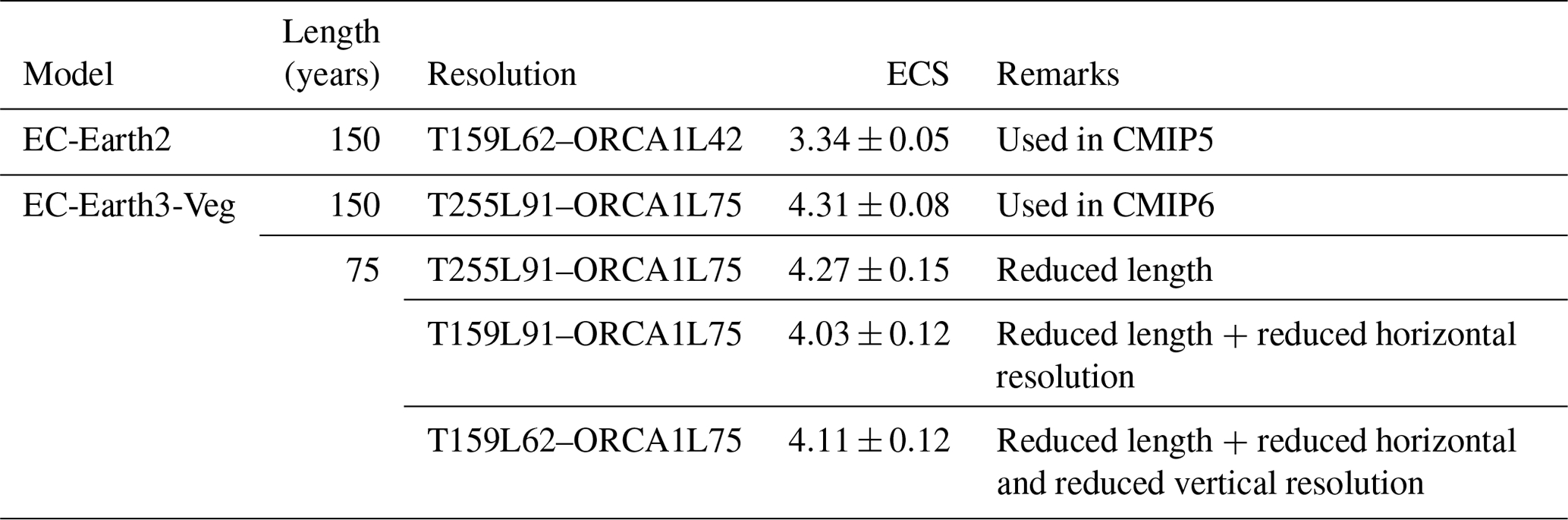
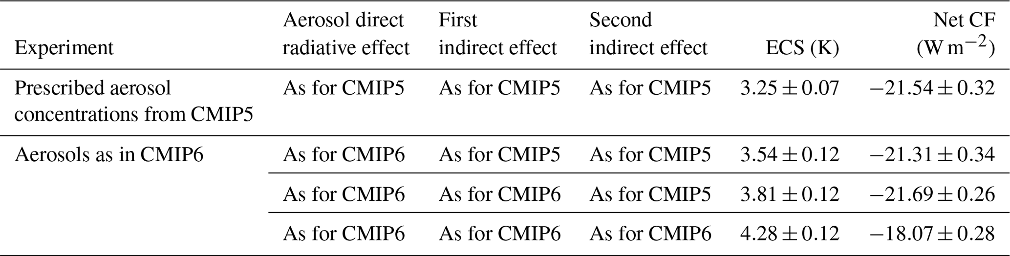
Table 4 Sensitivity of ECS and net CF to different realisations of the aerosol–cloud interaction processes. All experiments were carried out with the low-resolution (T159L62) configuration of EC-Earth3-Veg and stretch over only 75 years.

3.3 Reducing the model resolution

In another attempt to reduce the computational costs of the sensitivity simulations, we test if the horizontal and vertical resolution of ECE3 could be reduced to that of ECE2 (Table 3). In these tests we first change the resolution (only in the atmosphere) in the horizontal, and then we changed it in both the horizontal and the vertical. The ECS changes slightly from 4.3 to 4.2 K or stays close to 4.3 K when only the horizontal or both the horizontal and vertical resolution are changed. These changes in the ECS are small compared with the difference in ECS between ECE2 and ECE3. An important result of these tests is that the change in the resolution of the EC-Earth model from CMIP5 to CMIP6 is not responsible for the change in the climate sensitivity; thus, the reasons have to be sought elsewhere. Because the changes in the resolution only have a marginal impact on the ECS, the sensitivity experiments with modified aerosol–cloud interaction are carried out with the low-resolution configuration of EC-Earth3-Veg. The resulting ECS will not be fully accurate for the full-resolution CMIP6 model; nevertheless, the estimates obtained with the low-resolution configuration will allow us to make a qualitative assessment of the impact of the newly implemented aerosol scheme.

3.4 Sensitivity to the description of aerosols and their impacts on the cloud forcing

The results from a series of sensitivity experiments with the aerosol scheme in ECE3 are shown in Table 4. When reverting the newly implemented simple plume representation of MACv2-SP in combination with a pre-industrial background climatology back to the scheme with prescribed aerosol concentrations used for CMIP5, we find that the ECS drops to 3.25 K, which is close to the value that was found for the CMIP5 version of EC-Earth. Changing the source of the aerosol forcing from the CMIP5 dataset to the new representation of aerosol optical properties in CMIP6 but without aerosol indirect effects – the effective radius and autoconversion are parameterised as in the CMIP5 version of the model and do not depend on the number of activated aerosol particles calculated from the pre-industrial climatology of aerosol concentrations - the ECS increases slightly to 3.54 K. The change is small and not significant with all of the simplifications of the experimental design in mind. When the coupling between the explicit aerosol activation is switched on and impacts the effective radius (first indirect effect), the ECS increases further to 3.81 K; if the activated aerosol particles are also allowed to impact cloud microphysics, the ECS becomes 4.28 K. This last value is similar to the ECS from the CMIP6 experiments (4.31 K) with EC-Earth3-Veg performed at higher atmospheric resolution (T255L91).

This series of sensitivity experiments suggests that the increase in the ECS from CMIP5 to CMIP6 is mainly caused by the change in the representation of aerosol and their impacts on clouds and radiation. The implementation of MACv2-SP, as is suggested for CMIP6 models without an explicit aerosol scheme, has fundamentally changed the way that aerosols are prescribed in the model; however, this change has little effect on the ECS as long as the cloud droplet effective radius and autoconversion are independent of the aerosol concentration. The ECS increases when the more advanced treatment of the first and second indirect effects is introduced, with the largest contribution coming from the latter. This finding is further supported by the change in the net CF in these sensitivity experiments. The largest change in the CF is found when the second indirect aerosol effect is activated. In that case, the cooling by clouds becomes less strong (the CF increases) which reduces the feedback from the warming induced by the quadrupled CO₂ concentrations, resulting in a higher ECS.

Kiehl (2007) showed a correlation between stronger aerosol forcing and higher climate sensitivity in climate models. By introducing a more advanced treatment of aerosols in the ECE3 model and subsequent tuning to match a realistic pre-industrial equilibrium and present-day climate in the model, we may have altered the model's sensitivity. However, we have shown here that the ECS can also change without changing the model tuning. It is possible to regain the climate sensitivity of ECE2 with the new ECE3 model by reverting the changes in the representation of the aerosol cloud interaction without any retuning of ECE3.

4 Conclusions

The ECS of the EC-Earth model has increased from 3.3 K in CMIP5 to 4.3 K in CMIP6. In this work, we show that this increase can be explained by the revised description of aerosol processes when going from ECE2 to ECE3, in particular the implementation of the first and second indirect aerosol effects. In fact, cloud feedbacks were identified to be among the most important sources of uncertainty for the ECS for the past generation of climate models (Andrews et al., 2012). Interestingly, the analysis by Chylek et al. (2016) suggested that only CMIP5 models including indirect aerosol effects present a correlation between radiative forcing and equilibrium climate sensitivity similar to that discussed in Kiehl (2007).

Of course, the following questions have to be asked:

• How good is the representation of specific processes, such as the activation of aerosols, in ECE3?

• How realistic are the parameterisations of effective radius and autoconversion efficiency as a function of the activated cloud droplets?

• How will all these changes affect the ECS of the model?

The coming CMIP6 experiments in AerChemMIP will help us to better understand how well the ECE3 model represents such aerosol–cloud interactions. All results from this study are valid for the ECE3 model only. Many of the other climate models already had indirect aerosol effects in their CMIP5 version; therefore, they cannot easily explain an increase in the ECS with the introduction of a more sophisticated aerosol scheme. However, many models have updated their aerosol representation since CMIP5, and some models have implemented the new MACv2-SP scheme. It is possible – but impossible to prove here – that the changes in the aerosol treatment could have made a substantial contribution to the increase in ECS that many modelling groups have found.

The development of the next generation of the EC-Earth model has already begun. One of the lessons learnt from the large increase in the ECS when going from the CMIP5 to the CMIP6 version of the model is that we will have to carefully monitor the climate sensitivity (and other key metrics), not only at completion but also during the entire development process, as was done, for example, for the CESM2 model (Gettelman et al., 2019). Maintaining a well-tuned model version and concurrently having a continuous overview of the ECS evolution and the main feedback parameters over time will support us in the critical evaluation of any new model developments and will suggest a critical retuning of the model whenever important changes in climate sensitivity are found.