the Creative Commons Attribution 4.0 License.
the Creative Commons Attribution 4.0 License.
 | 21 Jul 2020
Development of the Community Water Model (CWatM v1.04) – a high-resolution hydrological model for global and regional assessment of integrated water resources management
Yusuke Satoh
Taher Kahil
Ting Tang
Peter Greve
Mikhail Smilovic
Luca Guillaumot
Fang Zhao
Yoshihide Wada
We develop a new large-scale hydrological and water resources model, the Community Water Model (CWatM), which can simulate hydrology both globally and regionally at different resolutions from 30 arcmin to 30 arcsec at daily time steps. CWatM is open source in the Python programming environment and has a modular structure. It uses global, freely available data in the netCDF4 file format for reading, storage, and production of data in a compact way. CWatM includes general surface and groundwater hydrological processes but also takes into account human activities, such as water use and reservoir regulation, by calculating water demands, water use, and return flows. Reservoirs and lakes are included in the model scheme. CWatM is used in the framework of the Inter-Sectoral Impact Model Intercomparison Project (ISIMIP), which compares global model outputs. The flexible model structure allows for dynamic interaction with hydro-economic and water quality models for the assessment and evaluation of water management options. Furthermore, the novelty of CWatM is its combination of state-of-the-art hydrological modeling, modular programming, an online user manual and automatic source code documentation, global and regional assessments at different spatial resolutions, and a potential community to add to, change, and expand the open-source project. CWatM also strives to build a community learning environment which is able to freely use an open-source hydrological model and flexible coupling possibilities to other sectoral models, such as energy and agriculture.
- Article
(14419 KB) - Full-text XML
-
Supplement
(2449 KB) - BibTeX
- EndNote


In recent years, the interactions between natural water systems, climate change, socioeconomic impacts, human management of water resources, and ecosystem management have increasingly been incorporated into the processes of large-scale hydrological models (Wada et al., 2017). Examples of these models are WaterGAP (Alcamo et al., 2003; Flörke et al., 2013), H08 (Hanasaki et al., 2008, 2018), MATSIRO (Pokhrel et al., 2012), LISFLOOD (De Roo et al., 2000; Udias et al., 2016), PCR-GLOBWB (Van Beek et al., 2011; Wada et al., 2014; Sutanudjaja et al., 2018), and SAFRAN-ISBA-MODCOU (Habets et al., 2008; Decharme et al., 2019). Human intervention in hydrology and water resources is becoming essential for the realistic simulation of global and regional hydrological processes. In particular, simulations of human water demands from different sectors such as agriculture, industry, and domestic could have a large impact on estimated hydrological storage (e.g., groundwater) and fluxes (e.g., discharge) (Alcamo et al., 2007; Wada et al., 2016). More efforts have gone into better groundwater representation in large-scale hydrological models to realistically simulate groundwater levels and surface–groundwater interactions (Pokhrel et al., 2015; Wada, 2016; Reinecke et al., 2019; de Graaf et al., 2015, 2017; Decharme et al., 2019).
In recent years, model intercomparison projects such as the WaterMIP (Water and Global Change Water Model Intercomparison Project) (Haddeland et al., 2011), Inter-Sectoral Impact Model Intercomparison Project (ISIMIP) (Warszawski et al., 2014), and the Coupled Model Intercomparison Project Phase 6 (CMIP6) (Eyring et al., 2016) led to, among other advantages, a systematic overview of models, a consistent database of spatial input data and simulation protocols and scenarios, and a shared database of results, all of which facilitate analysis across different modeling sectors (e.g., water, agriculture, energy, biome, and climate). This has also led to a better understanding of how to assess future changes in land use and climate in relation to water resource constraints under given uncertainties of the forcing drivers such as climate.
Clark et al. (2011) and Bierkens (2015) indicate that model intercomparison efforts have failed to lead to a better understanding of the origins and consequences of systematic model bias and differences and thus to an improved outcome of model components. Bierkens (2015) argues that while there are many catchment hydrological models for specific catchments specializing in their own sophisticated model parameterizations, few global hydrological models – compared with the number of regional hydrological models – interact with these regional models and modeling groups (e.g., Siderius et al., 2018). One way of overcoming this barrier could be to implement multiple modeling or modular approaches into the unifying framework suggested by Clark et al. (2015). Thus, we here develop a new large-scale hydrological and water resources model, the Community Water Model (CWatM), which has a flexible modular structure and unique global and regional spatial representations. Because of complex interactions of hydrology with food, energy, and ecosystems, it is expected that hydrological models can cover these interactions as model components. To advance the move from large-scale hydrological models to better model representations of hydrological processes, we believe that it is also necessary to create a community-driven modeling environment that facilitates the exchange of ideas, components or modules, data, and results in an easily communicable format. In a wider sense, a user-friendly and flexible model structure will enable more active engagement with stakeholders and associated capacity training.
Therefore, CWatM includes the features detailed below:
-
use of an open-source platform as a way to exchange ideas and develop model codes that facilitate capacity enhancement, especially in regions with limited access to high-performance computing facilities and high-resolution data;
-
scalability to allow use of the model at the regional-to-catchment scale and also at the continental-to-global scale, which facilitates learning between global and regional hydrological model applications;
-
use of a flexible modular structure to explore the linkages with other sectoral models such as those relating to land use, agriculture, and energy so that options and the solution space can be integrated;
-
existing linkages to state-of-the-art models for energy (MESSAGE) (Sullivan et al., 2013), land use and ecosystems (GLOBIOM) (Havlík et al., 2013), agriculture (IIASA-EPIC) (Balkovič et al., 2014), water quality (MARINA) (Strokal et al., 2016), and the hydro-economy (ECHO) (Kahil et al., 2018); and
-
linkages to the political economy and stakeholder perspectives (Tramberend et al., 2020), e.g., social hydrology (Sivapalan et al., 2012; Seidl and Barthel, 2017).
A model software architecture includes the aspects below:
-
a high-level programming language for easy comprehension of the code and to facilitate extensibility;
-
an interface to a fast computing language (e.g., C) for time-intensive operations (e.g., river routing);
-
a multiplatform to adjust the model to the users' needs and capacity (e.g., Windows, Linux, Mac, and high-performance clusters and supercomputers);
-
a high level of modularity to be extensible for different model options to solve the same process, e.g., evaporation with Hargreaves, Hamon, Penman–Monteith, or for a different purpose (e.g., flood forecasting, water–food nexus, linking to hydro-economic modeling);
-
documentation of the model and the source code in a semiautomatic way to facilitate immediate documentation and comprehension of the concepts involved; and
-
a state-of-the-art data structure for reading and writing spatiotemporal data to allow for efficient management of data storage and facilitate the development toward high-resolution models.
As described above, the main novelty of CWatM lies not in providing entirely new concepts for modeling hydrological and socioeconomic processes but in combining existing good practice in various scientific communities beyond hydrology itself. CWatM has a modular model structure which is open source and uses state-of-the-art data storage protocols as input and output data. Currently, CWatM can use different spatial resolutions from 30 arcmin (∼50 km by 50 km at the Equator) to 30 arcsec (∼1 km by 1 km), enabling it to address both global and regional water management. The online user manual and automatic source code documentation make CWatM an easy-to-use tool which can be integrated and coupled to other toolsets such as land use modeling and hydro-economic modeling. CWatM also strives to build up a community which can freely use an open-source hydrological model with the possibilities of coupling it to other water management models such as WEAP (Yates et al., 2005) and ECHO (Kahil et al., 2018).
This paper describes the development of the model, including its structure and modules, and gives some examples of applications. Section 2 of this paper presents a detailed description of the model development of CWatM. Section 3 describes the data used for the model. Section 4 introduces the calibration of the model. Section 5 shows results for several calibrated catchments and two application examples. Section 6 shows how CWatM is linked to other sectoral models. Section 7 discusses the conclusions and the way forward.
2.1 Model concept
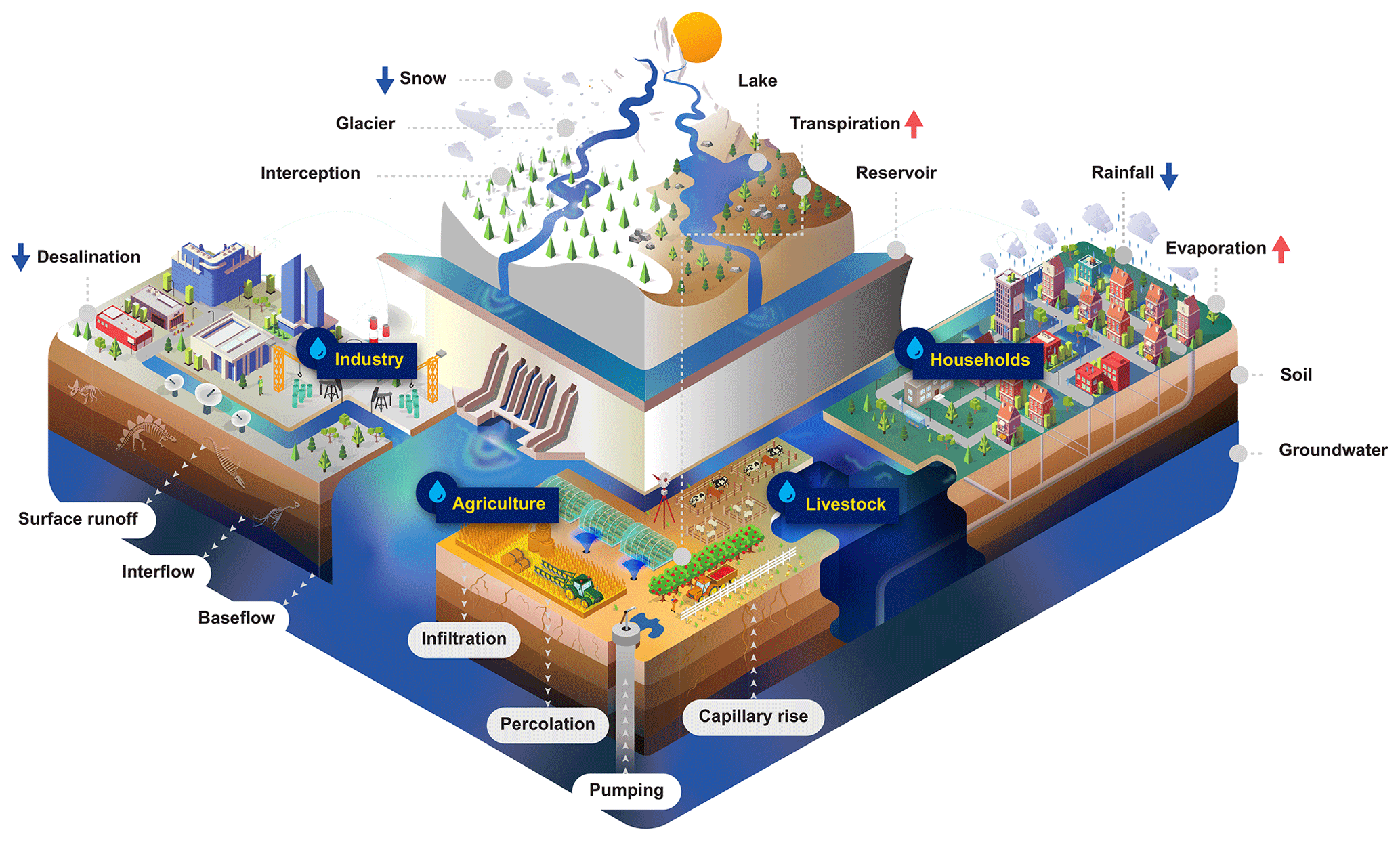
The Community Water Model (CWatM) is an integrated hydrological and channel routing model developed at the International Institute for Applied Systems Analysis (IIASA). CWatM quantifies water availability, human water use, and the effect of water infrastructure, e.g., reservoirs, groundwater pumping, and irrigation, in regional water resources management. A schematic view of the processes is given in Fig. 1. CWatM is a grid-based model, and its recent version has spatial resolutions of 0.5∘ and 5′ (with subgrid resolution taking into account topography and land cover) at daily temporal resolution (with subdaily time stepping for soil, lakes and reservoirs, and river routing). The model can also be applied at 30 arcsec. CWatM follows a modeling concept similar to that of large-scale hydrological models such as H08 (Hanasaki et al., 2006, 2008, 2018), WaterGAP (Alcamo et al., 2003; Flörke et al., 2013), LPJmL (Bondeau et al., 2007; Rost et al., 2008), LISFLOOD (De Roo et al., 2000; Burek et al., 2013), PCR-GLOBWB (Van Beek et al., 2011; Wada et al., 2014; Sutanudjaja et al., 2018), VIC (Xu et al., 1994), MHM (Samaniego et al., 2011; Kumar et al., 2013), and HBV (Bergström and Forsman, 1973; Lindström, 1997). A comprehensive overview of existing global hydrological models (GHMs) is given in Bierkens (2015), Kauffeldt et al. (2016), Pokhrel et al. (2016), Wada et al. (2017), and in the ISI-MIP project (Frieler et al., 2016), with the latter having been used for model comparison of different GHMs. Among these large-scale hydrological models, CWatM uses a model implementation similar to that of PCR-GLOBWB and LISFLOOD. The philosophy of CWatM is the same as that described in Bergstrom (1991) for the model HBV: as complex as necessary but not more. This means that the model merges conceptual and physical modeling and is keeping a similar level of physical complexity throughout the model. If a higher-detail physical model is needed, it should be introduced as add-on modules. For different tasks, different interactions to other models and different descriptions of processes are needed.
The CWatM modeling system is written in Python 3.7 with only a few Python packages (numpy, scipy, gdal, netCDF4) and can be used on different platforms (Unix, Linux, Windows, Mac). Excessive computational parts can be added via an interface as C or Fortran code. For example, runoff concentration within a grid cell or river routing using the kinematic wave equation is done in C. With this approach the advantage of high-level languages like Python to write and understand code quickly and effectively and the advantage of languages like C for fast computing are preserved. The focus of the model development is to build a flexible model architecture and to present a full hydrological model for calculating water availability and demand. The model can handle different spatial resolutions from 1 to 50 km at a daily temporal resolution for different tasks from global to regional assessments.
The target audience of the model is hydrological modelers of varying levels of programming familiarity. Modelers with no experience in programming languages like Python can simply use the executable together with the settings file. Modelers with only limited experience in Python can use the platform-independent Python version with no need to adapt the source code itself. Finally, modelers with programming capacity in Python can engage with the source code and adapt the model to their specific needs. The wide adoption of Python as a programming language and the open-source approach will allow for a community of developers to engage with and further develop CWatM. The code itself comes with a GNU General Public License and is hosted on GitHub (https://github.com/CWatM/CWatM, last access: 27 June 2020), where every change is trackable and transparent. The source code is programmed in the modern programming language Python, with only certain computationally demanding parts written in C, such as river routing. Each subroutine is documented for its design and purpose, and 40 % of the source code lines is documentation. CWatM follows a modular development pathway in several ways, which simplifies the use of the model for the different user groups. Firstly, the program is independent from the settings file, which includes all information related to data, parameters for each process, and output options. This enable the user to run the model without any understanding of Python, while still providing flexibility of input and output options to the user. Secondly, the modules for hydrological processes and data handling (e.g., reading configuration, data read and write routines, error handling) are handled separately; further, the different hydrological processes (from calculation of potential evaporation to river routing) are each handled independently. This enables the advanced user to concentrate on adapting specific processes or develop their own hydrological modules to extend the modular structure (see Fig. S11 in the Supplement for the CWatM modular structure). Thirdly, each module is identically composed of an initialization class and a dynamic class operating through time; this structure is motivated by the PC-Raster framework (Karssenberg et al., 2010). Alternative descriptions of processes (e.g., Hargreaves instead of Penman–Monteith for calculating potential evaporation) can be included in a module as different initial and dynamic classes, and the selection of the specific process representation can be selected in the settings file. Linking to other models can be done by transfer via input and output files, where every global variable of CWatM (examples include evapotranspiration, lake and reservoir storage, etc.) can be written as annual, monthly, or daily time series as text files for specific points, aggregated to basins, or as maps showing the value for each cell. Any variable can have a meta information entry. This enables a simplified linking to other models (e.g., hydro-economic) which might need only, for example, monthly values of groundwater recharge per basin. Linking to models like the land use model GLOBIOM is done with pre- and postprocessing coupler functions, as most of these models need aggregated data as ASCII files. Coupling to MODFLOW (McDonald and Harbaugh, 1988; Harbaugh, 2005) is done by using the FloPy Python package (Bakker et al., 2016). The user can switch on the MODFLOW coupling in the settings file and in addition the necessary data for the groundwater model (e.g., transmissivity maps) have to be provided. Coupling to models using C can be done by an in-memory coupling using the ctypes library, as this is already done to embed the kinematic wave routing routine. CWatM generally accepts netCDF, Geotiff, and PCRaster input maps and uses netCDF4 formats for outputs and to store spatiotemporal data efficiently. This also allows for meteorological forcing data to be used without the need for reformatting. NetCDF4 also has the advantage that the metadata are directly attached. CWatM uses the Climate and Forecast (CF) Metadata Convention 1.6. Metadata information (unit, long name, standard name, author, etc.) can be included for every output netCDF file by adding this information to the file metanetcdf.xml. Finally, to best support and reach its community, CWatM has a Google group and forum (https://groups.google.com/d/forum/cwatm, last access: 27 June 2020); online documentation (https://cwatm.iiasa.ac.at, last access: 27 June 2020) including model setup basics, data information, and license information; and uses Sphinx (https://www.sphinx-doc.org, last access: 27 June 2020) for the auto-documentation of source code.
The model is accessible and customizable to the needs of different users with varying levels of programming skill, allowing for research questions of varying spatial scales from global to local scales to be answered. This will support and enable different stakeholder groups and scientific communities beyond hydrology and of varying capacities to engage with a hydrological model and support their investigations (see Sect. 6). We hope that we have appropriately represented CWatM and its use of best practices in research software as stated in Wilson et al. (2014) and Jiménez et al. (2017). CWatM was already used in several scientific assessments, including Wang et al. (2019a, b), He et al. (2019), Vinca et al. (2019), and Kahil et al. (2020), and has a small but growing community of users in several countries around the world.
2.2 General overview of the hydrological processes
CWatM can use different datasets of daily meteorological forcing as inputs to calculate potential evaporation with Penman–Monteith (Allen et al., 1998) as a default option, as well as other methods such as the Hargreaves (Hargreaves and Samani, 1958) and Hamon (Hamon, 1963) approaches. Elevation data on the subgrid level and temperature are used to split precipitation into rain and snow, while the degree-day factor method (WMO, 1986) calculates snow melt.
CWatM calculates the water balance for six land cover classes separately (forest, irrigated, paddy-irrigated, water covered, sealed area, and “other” land cover class). Soil processes, interception of water, and evaporation of intercepted water are calculated separately for four different land cover classes (forest, irrigated, paddy-irrigated, and other), and the resulting flux and storage per grid cell is aggregated by the fraction of each land cover class in each grid cell. Infiltration into the soil is calculated with the Xinanjiang model approach (Zhao and Liu, 1995; Todini, 1996). The model calculates preferential bypass flow which bypasses the soil layers and percolates directly to groundwater, similar to the approaches of LISFLOOD (Burek et al., 2013), VarKast (Hartmann et al., 2015), and HBV (Lindström et al., 1997). Soil moisture redistribution in three soil layers is calculated using the Van Genuchten simplification (Van Genuchten, 1980) of the Richards equation. The depth of the first soil layer is fixed at 5 cm so that its soil moisture can be compared with products from remote sensing data. The second and third soil layer depths depend on the root zone depth of each land cover class and the total soil depth from data of the Harmonized World Soil Database 1.2 (HWSD) (FAO et al., 2012). Water uptake and transpiration by vegetation are based on an approach by Supit et al. (1994) and Supit and van der Goot (2003), where water stress reduces the maximal transpiration rate. Direct evaporation from the soil surface is calculated separately for two more land cover classes, namely, water and sealed (impermeable) surface; evaporation and runoff are also calculated separately.
Groundwater storage is modeled using a linear reservoir. In the newest version of the model, a MODFLOW coupling is also available, allowing users to include lateral flows between grid cells. Capillary rise from groundwater to the soil layers is included. Runoff concentration in a grid cell is calculated using a triangular weighting function. CWatM applies the kinematic wave approximation of the Saint-Venant equation (Chow et al., 1998) for river routing.
Lakes and reservoirs are included in two different ways: (i) a lake or reservoir has an upstream area beyond the actual grid cell and is part of the grid linking the river routing system and (ii) a lake or reservoir is only a part of the regional river system within a grid cell. Reservoirs are simulated using a simple general reservoir operation scheme as used in LISFLOOD (De Roo et al., 2000; Burek et al., 2013). Lakes are simulated by using the modified Puls approach (Chow et al., 1998; Maniak, 1997).
Water demand and consumptions are estimated for the livestock, industry, and domestic sectors using the approach of Wada et al. (2011). Water demand and consumption for irrigation and paddy irrigation are calculated within CWatM using the crop water requirement methods of Allen et al. (1998). This irrigation scheme can also dynamically link the daily surface and soil water balance with irrigation water.
With these coupled processes, CWatM can facilitate assessment of the changing pattern of water supply and demand across scales under climate change at different spatial resolutions. The modular structure also makes the linking of CWatM with other IIASA models possible, e.g., MESSAGE (Sullivan et al., 2013), GLOBIOM (Havlík et al., 2013), and ECHO (Kahil et al., 2018, 2019), to develop an integrated assessment modeling framework for nexus issues (e.g., water–food–energy) or hydro-economic modeling for quantifying water infrastructure investment options for regional water resources management.
2.3 Methods
2.3.1 Meteorological forcing
CWatM is able to use different datasets of meteorological forcing for the current climate – e.g., MSWEP (Beck et al., 2017), WFDEI (Weedon et al., 2014), PGMFD (Sheffield et al., 2006), GSWP3 (Kim et al., 2012), or EWEMBI (Lange, 2018) – or future climate projections from different general circulation models (GCMs) (e.g., data from ISIMIP project, Frieler et al., 2016). CWatM can use the netCDF4 repositories of original meteorological forcing without reformatting. As long as the forcing data are using the CF 1.6 Convention, CWatM takes care of the different names of the input variables and divides the dataset for the catchment or global scale, depending on a mask map or predefined rectangular selection. The forcing data are automatically regridded to the model grid (e.g., 30′′ or 5′) using the delta change method (Moreno and Hasenauer, 2016; Mosier et al., 2018) based on high-resolution monthly data from WorldClim version2 (Fick and Hijmans, 2017).
Depending on the method used for calculating potential evaporation, e.g., Penman–Monteith method (Allen et al., 1998), Hargreaves method (Hargreaves and Samani, 1958), or Hamon method (Hamon, 1963), different climate data are needed. As a default, the Penman–Monteith needs as inputs precipitation; humidity; long- and short-wave downward surface radiation fluxes; maximum, minimum, and average 2 m temperature; 10 m wind speed; and surface pressure. Temperature data are additionally needed to distinguish between snow and rain.
2.3.2 Potential evaporation
Potential reference crop evaporation rate (ET0) is calculated from a hypothetical reference vegetation with specific characteristics and unlimited availability of water (Allen et al., 1998). In the same way, the potential evaporation of an open water surface (EW0) is calculated. ET0 and EW0 are treated as pure climatic variables, because for calculation purpose they are not influenced by land cover or soil properties. In reality, the potential evapotranspiration might be different to ET0 due to differences in vegetation characteristics, aerodynamic resistance, or surface reflectivity (albedo). To account for the variability of vegetation, ET0 is multiplied by an empirical “crop coefficient” (kcrop) that lumps these differences into one factor, yielding a potential crop evapotranspiration rate (ETcrop). The method used here is based on work described in Allen et al. (1998) and Supit and van der Goot (2003).
2.3.3 Snow and frost
Precipitation is split into rainfall and snow, depending on the temperature. If the average temperature is below 1 ∘C (default, but can be changed), all precipitation is assumed to be snow. For large grid cells, e.g., 0.5∘ or 5′ resolution, there is a considerable subgrid heterogeneity in elevation and therefore in temperature and snow accumulation and melt (Anderson, 2006). Because of this, snow accumulation and melt are modeled in up to 10 separated elevation zones on the subgrid level using different elevation zones and a fixed, defined moist adiabatic lapse rate.
Snow accumulates until it melts or evaporates. The rate of snowmelt is estimated using a degree-day factor method, which take into account the fact that snowmelt increases when it is raining (Speers and Versteeg, 1979):
where M is snowmelt per time step (mm), R is rainfall intensity (mm d−1), Δt is time interval (d), Tm is equal to 0 ∘C, Cm is the degree-day factor (mm ∘C−1 d−1), and CSeasonal is the seasonal variable melt factor.
CSeasonal is a factor depending on the day of the year, which varies the snow melt rate. A similar factor is used in several other models (e.g., Anderson, 2006; and Viviroli et al., 2009). At high altitudes the model tends to accumulate snow without any melting loss, because temperature never exceeds 1 ∘C. In these altitudes snow is accumulated and is converted into firn, which is then converted into ice as glaciers move to lower regions over decades or even centuries. In the ablation area, the ice is again melted. In CWatM this process can be optionally simulated by melting the snow at higher altitudes on an annual basis over summer using a higher degree-day factor and temperature from a lower subgrid zone. Hydrological processes occurring near the soil surface are affected and halted if the soil surface is frozen. To estimate whether the soil surface is frozen, a frost index F is calculated to estimate whether the soil surface is frozen based on Molnau and Bissell (1983). The frost index changes by day at a rate given by
where dF∕dt is given (∘C d−1), Af is the decay coefficient (here 0.97 d−1), K is snow depth reduction coefficient (here 0.57 cm−1), ds is grid average of depth of the snow cover (mm equivalent water depth), and wes is snow water equivalent.
For each time step, the value of F (∘C d−1) is updated as
The soil is considered frozen when the frost index is above a critical threshold of 56; then, every soil process in the first two layers will be stopped. Precipitation bypasses soil and is transformed into surface runoff until the frost index is again lower than 56.
2.3.4 Interception, evaporation from soil, open water, and sealed surface
The calculation for interception and evaporation is based on Allen et al. (1998). For each land cover class, a maximum interception storage is defined. Interception storage can be filled by rainfall and depleted by evaporation using potential evaporation from open water. The leftover interception storage is added to the water available for infiltration in the other time step. Evaporation from soil is calculated using the potential reference evapotranspiration rate multiplied by a soil crop factor (default: 0.2). Evaporation from sealed area or open water is calculated using the potential evapotranspiration for the open water rate multiplied by a factor (defaults: 0.2 for sealed, 1.0 for water).
2.3.5 Transpiration from plants
Potential transpiration from plants is calculated using the potential reference evapotranspiration multiplied by a crop-specific factor available as a spatially distributed dataset for each land cover type for every 10 d over a year. The crop coefficient is aggregated from MIRCA2000: a global dataset of monthly irrigated and rainfed crop areas (Portmann et al., 2010). The actual transpiration rate depends on the available water and on the ability of the crop type to deal with water stress. The energy already used up for the evaporation of intercepted water is subtracted here in order to respect the overall energy balance. The actual transpiration rate is reduced by a water stress factor which takes into account the ability of the crop to deal with water stress and an index of water stress of the soil:
where rws is the reduction factor because of water stress, w1 is soil moisture in the two upper soil layers (mm), wwp1 is soil moisture at wilting point (soil moisture potential pF 4.2), and wcrit1 is soil moisture below which water uptake is reduced and plants start closing their stomata.
The critical amount of soil moisture is calculated as
where p is soil depletion fraction; wfc1 is soil moisture at field capacity; and Cropgroup number is the crop group number, which is an indicator of adaptation to dry climate (e.g., olive groves are adapted to dry climate and can therefore extract more water from soil that is drying out than rice can).
The actual transpiration Ta is calculated as
The procedure for estimating p and Rws is described in detail in Supit and van der Goot (2003).
2.3.6 Infiltration into soil and preferential bypass flow
To estimate the infiltration capacity of the soil, the approach of Xinanjiang (also known as VIC/ARNO model) (Zhao and Liu, 1995 and Todini, 1996) is used. The saturated fraction of a grid cell that contributes to surface runoff is related to the overall soil moisture of a grid cell through a nonlinear distribution function. The saturated fraction As is approximated by the following distribution function:
where ws1 and w1 are the maximum and actual soil moisture in the upper two soil layers and b is an empirical shape parameter.
To simulate the preferential bypass flow of the soil, a fraction of the water available for infiltration is passed directly to the groundwater zone. The fraction is calculated as a function of the relative saturation of the first two soil layers.
where Dpref,gw is preferential flow per time step, Wav is available water for infiltration, and cpref is empirical shape parameter.
A preferential flow component that lets more water bypass the soil as the soil gets wetter is calculated.
The actual infiltration INFact is calculated as
2.3.7 Soil moisture redistribution and capillary rise
Unsaturated flow and transport processes can be described with the 1D Richard equation, which requires a high spatiotemporal distribution of the soil's hydraulic properties and a numerical solver.
where θ is soil volumetric moisture content [L3L−3], t is time [T], h is soil water pressure head [L], K(θ) is unsaturated hydraulic conductivity [LT−1], z is vertical coordinate, and S is the source–sink term [T−1]
In order to apply an analytical and faster solution, Van Genuchten (1980) hydraulic functions based on the model of Mualem (1976) were adopted. It assumes a matric potential gradient of zero, which implies a flow that is that is always in a downward direction at a rate equal to the conductivity of the soil, and free drainage as the lower boundary condition in the lowest soil layer. The relationship between hydraulic conductivity and soil moisture status is described by the Van Genuchten (1980) equation.
where Ks is saturated conductivity of the soil (m d−1); K(θ) is unsaturated conductivity; Θ, θs, and θr are the actual, maximum, and residual amounts of moisture in the soil (m); and m is calculated from the pore-size index (λ): .
The soil hydraulic parameters Θ, θs, θr, λ, and Ks are needed to simulate soil water transport for the Van Genuchten model and are derived via a pedotransfer function (e.g., model Rosetta of Zhang and Schaap, 2017) from standard soil properties (soil texture, porosity, organic matter, and bulk density).
Once the unsaturated conductivity for each soil zone is determined, the water flux to the next zone can be estimated. At a time step of 1 d and high K(θ), the vertical flux can exceed the available soil moisture:
Therefore, the soil moisture equation has to be solved iteratively on a subdaily time step.
Capillary rise occurs only when the groundwater level is close to the surface. CWatM estimates the total fraction of the area with groundwater level of between 0 and 5 m from the surface in discrete steps and calculates the flux from groundwater to the soil layer based on unsaturated conductivity and field capacity (Wada et al., 2014).
2.3.8 Groundwater
Groundwater storage and baseflow are modeled using a linear reservoir approach as in LISFLOOD (De Roo et al., 2000; Udias et al., 2016). The groundwater zone is filled by the water percolating from the lower soil zone and the preferential flow and is emptied by capillary rise and baseflow. The outflow from the groundwater zone is given by
where Qbase is baseflow or outflow from the groundwater zone, Tbase is a groundwater reservoir constant in days, Storage is water stored in the groundwater zone, and Rcoeff is a recession coefficient of the groundwater zone.
For considering lateral fluxes among grid cells and the explicit computation of groundwater levels over finer spatial domains, CWatM has an option to couple with MODFLOW (McDonald and Harbaugh, 1988, Harbaugh, 2005) using the FloPy Python package (Bakker et al., 2016) in a similar way to PCR-GLOBWB (Sutanudjaja et al., 2014). The 5′ resolution version of CWatM is coupled with a one-layer MODFLOW model at a finer MODFLOW resolution (from 4 km to 400 m) with the aim of integrating the small-scale topographic control. The coupling is made on a daily to weekly base water balance.
CWatM simulates the vertical soil water flow in three soil layers, while MODFLOW simulates lateral groundwater flows. CWatM-MODFLOW is technically coupled (using the Drain package) via capillary rise from groundwater to the soil zones, groundwater recharge from the soil zones, and baseflow outflow from groundwater to the river network system. As the MODFLOW resolution can be smaller than the CWatM resolution, the CWatM mesh is subdivided into two parts: one part where groundwater recharge occurs and one part where capillary rise from groundwater occurs. The area of each part is determined by the percentage of MODFLOW cell, where the water level reaches the lower soil layer inside a CWatM mesh. To distinguish whether the groundwater flow to the surface will be attributed to capillary rise or baseflow, a percentage of rivers is attributed to each MODFLOW cells and calculated based on a 200 m resolution topographic map. Aquifer properties, like transmissivity or aquifer thickness, are estimated using the approach of de Graaf et al. (2015) and Gleeson et al. (2011). The results presented in Sect. 5 of this work are calculated using the simplified linear reservoir approach.
2.3.9 Runoff concentration within a grid cell
The process between runoff generation and river routing for each grid cell is called runoff concentration. The runoff generated from each cell is routed to the corner of each cell. Depending on land cover class, slope, and runoff group (surface, interflow, or baseflow), a concentration time (peak time) is determined. The total runoff for a grid cell is then calculated using a triangular weighting function.
where Q(t) is the total runoff of a grid cell of a time step, runoff is the runoff component (surface, interflow, baseflow), Qrunoff is the runoff of land cover class of a runoff component, t is time (1 d), and c(i) is a triangular function:
2.3.10 River routing
Flow through the river network is simulated using kinematic wave equations. The basic equations used are the equations of continuity and momentum. The continuity equation is
where Q is channel discharge (m3 s−1), A is cross-sectional area of the flow (m2), and q is the amount of lateral inflow per unit flow length (m2 s−1).
The momentum equation can also be expressed as in Chow et al. (1998):
The coefficients α and β are calculated by putting in Manning's equation. This leads to a nonlinear implicit finite-difference solution of the kinematic wave if you transform the right side:
where J is time index, I is the space index, and α and β are coefficients.
With the coefficients α and β, the nonlinear equation can be solved for each grid cell and for each time step using an iterative approach given in Chow et al. (1998). The coefficients can be calculated using Manning's equation.
where n is Manning's roughness coefficient, P is wetted perimeter of a cross section of the surface flow (m), and S0 is the topographical gradient.
Solving this for α and β gives
where P is the wetted perimeter approximated in CWatM: P equals channel width plus 2 times the channel bankfull depth, n is Manning's coefficient, and S0 is gradient (slope) of the water surface: S0 equals the change in elevation divided by the channel length.
To calculate α, CWatM uses a fixed network depending on the spatial resolution, and, for each grid cell, the channel width, depth, length, gradient, and Manning's roughness have to be known. As water can travel a distance greater than a cell size in 1 d, river routing and the lake and reservoir routines are performed on a subdaily time step, based on the chosen spatial resolution.
2.3.11 Reservoirs and lakes
Reservoirs and lakes (RL), based on the HydroLakes database (Messager et al., 2016; Lehner et al., 2011), are simulated as part of the channel network. Using the approach of Hanasaki et al. (2018) and Wisser et al. (2010), we distinguish between global RL and local RL. Global RL are located in the main channel of a grid cell with a catchment upstream of this grid cell. Local RL are more or less situated inside one grid cell at the tributaries of the main channel and not attached to the main river. Local RL are defined in CWatM depending on the spatial resolution. All RL with an RL area of less than 200 km2 at 0.5∘ (5 km2 for 5′) or with a watershed of less than 5000 km2 at 0.5∘ (200 km2 for 5′) are defined as “global” RL. The approach for calculating water storage and outflow of RL is the same for local and global RL, but the retention effect of local RL will be calculated during the runoff concentration process within a grid cell, while the effect of global RL will be calculated during the river routing process and includes the whole river network of a catchment.
Reservoir operation method
The method of simulating reservoir operations is taken from LISFLOOD (Burek et al., 2013). A total storage capacity S is assigned to each reservoir, and the fraction of filling of a reservoir is calculated. Three filling levels are defined. (a) The “conservative storage limit” fraction because a reservoir should never be completely empty (default set to 10 % of the total storage). For prevention of damage in case of flooding, a reservoir should not be filled to the full storage capacity. (b) The “flood storage limit” (Lf) represents this maximum allowed storage fraction (default set to 90 % of the total storage); (c) the “normal storage limit” (Ln) defines the buffering capacity and the available storage of a reservoir between Ln and Lf.
Another three parameters define how the outflow of a reservoir is regulated. (a) Each reservoir has a “minimum outflow” Omin. The default is set to 20 % of the average discharge, e.g., for ecological reasons. (b) A maximum possible outflow or the “non-damaging outflow”, Ond, is defined which causes no problems downstream in case of flood. The default for this outflow is set to 400 % of the average discharge. (c) Between the state of flood and normal storage limit, a reservoir is managed as much as possible to deliver a constant outflow so that there is also a constant energy output from hydropower generation. “Normal outflow”, Onorm, is set as a default value to average discharge.
The outflow Ores, is calculated depending on the fraction of the filling of the reservoir as
where S is reservoir storage capacity (m3), F is reservoir fill fraction (1 at total storage capacity) (–), Lc is conservative storage limit (–), Ln is normal storage limit (–), Lf is flood storage limit (–), Omin is minimum outflow (m3 s−1), Onorm is normal outflow (m3 s−1), Ond is non-damaging outflow (m3 s−1), and Ires is reservoir inflow (m3 s−1).
Lake method
Lakes are simulated using the modified Puls approach (Chow et al., 1998, Maniak, 1997) similar to the approach as in LISFLOOD (Burek et al., 2013). As lake inflow, the channel flow upstream of the lake location is used. As lake evaporation, the potential evaporation rate of an open water surface is taken. The modified Puls approach assumes that lake retention is a special case of flood retention with horizontal water level and the equations of river channel routing (see Sect. 2.3.10, “River routing”) can be written as
where QIn1 is inflow to lake at time 1 (t), QIn2 is inflow to lake at time 2 (t+Δt), QOut2 is outflow from lake at time 1 (t), QIn2 is outflow from lake at time 2 (t+Δt), S1 is lake storage at time 1 (t), and S2 is lake storage at time 2 (t+Δt).
The change in storage is inflow minus outflow and open water evaporation. The equation is solved by calculating the lake storage curve as a function of sea level, S=f(h), and the rating curve as a function of sea level, Q=f(h). Lake storage and discharge are linked by the water level.
The assumptions made here to simplify the equation are the following.
-
A modification of the weir equation by Poleni from Bollrich and Preißler (1992) is assumed:
-
If the weir does not have a rectangular form but a parabola form, the equation can be simplified to
-
The lake storage function is simplified to a linear relation:
where S is lake storage, A is lake area, and H is sea level.
2.3.12 Water use module
Irrigation water demand
Irrigation is by far the biggest consumer of water at around 70 % of global gross water demand (Döll et al., 2009). Irrigation water demand is calculated by following the method developed in PCR-GLOBWB (Wada et al., 2011, 2014) using the MIRCA2000 crop calendar of Portmann et al. (2010) and irrigated areas from Siebert et al. (2005) to account for seasonal variability, different crops, and different climatic conditions. MIRCA2000 explicitly considers multiple cropping. The associated crop- and stage-specific crop coefficients are derived from the Global Crop Water Model (Siebert et al., 2010). The crops are then aggregated into paddy and non-paddy and the crop coefficients are similarly aggregated by weighing the area of each crop class. Then, the cell-specific crop coefficient as it changes in time is related to the crops growing in this cell, inclusive of multiple cropping considered in the MIRCA2000 dataset. We refer to Wada et al. (2014) for the detailed descriptions. In brief, irrigation and water withdrawal and consumption are calculated separately for paddy (rice) irrigation and irrigation of other crops. To represent flooding irrigation of paddy fields, a 50 mm surface water depth is maintained until a few weeks before the harvest. Paddy irrigation demand is a function of the storage change of the surface water layer, net precipitation, infiltration to lower soil layers, and open water evaporation from the surface water layer. For non-paddy irrigation, the irrigation demand is calculated using the difference between total and available water in the first two soil layers where total water is equal to the amount of water between field capacity and wilting point and available water is equal to the amount of water between current status and wilting point. Water withdrawal is calculated using the water efficiency rate of FAO (2012) and Frenken and Gillet (2012).
Livestock water demand
Livestock water demand is assumed to be the same as livestock water consumption and is calculated by the number of livestock in a grid cell with the daily drinking water requirement per individual livestock type (six livestock types in total) and per air temperature for seasonal change in drinking water requirement. The approach is taken from Wada et al. (2011).
Industrial and domestic water demand
Calculation of industrial water demand also follows the method of Shen et al. (2008) and Wada et al. (2011) using the gridded industrial water demand data for 2000 from Shiklomanov (1997) and multiplying it by water use intensity. Water use intensity is a function of gross domestic product (GDP), electricity production, energy consumption, household consumption, and a technological development rate per country. Domestic water demand is calculated by multiplying the population in a grid cell by a country-specific per capita domestic water withdrawal rate taken from FAO (2007) and Gleick et al. (2009). Adjustments for air temperature and for country-based economic and technological development are carried out based on the approach of Wada et al. (2011).
Water withdrawal and return flows
The approach for calculating water withdrawal from different sources, water consumption, and return flows is based on the work of de Graaf et al. (2014), Wada et al. (2014), Sutanudjaja et al. (2018), and Hanasaki et al. (2018). Water demand can be fulfilled by surface water and groundwater. Based on the work of Siebert et al. (2010), groundwater for irrigation can be only used in areas that are equipped for irrigation. Groundwater is, at first, only abstracted from the renewable groundwater storage. Water demand that cannot be fulfilled purely from groundwater uses surface water from rivers, reservoirs, and lakes. An environmental flow cap can be set in order to sustain environmental needs for rivers, reservoirs, and lakes. If water demand still cannot be fulfilled, additional water is taken from nonrenewable groundwater. At 5′ resolution, water demand cannot always be covered by surface or groundwater resources in the same grid cell; therefore, CWatM uses the approach of LISFLOOD (Burek et al., 2013) and takes water from up to five grid cells downstream moving along the local drainage direction.
Return flow and associated losses (i.e., conveyance, application) are calculated using the approaches of LPJmL (Rost et al., 2008) and H08 (Hanasaki et al., 2018). Return flow is the flow which is withdrawn from surface water or groundwater but is not consumed. For the return flow rate, we follow the approach of Hanasaki et al. (2018). For irrigation, the return flow is calculated using the irrigation efficiency by Döll and Siebert (2002). For domestic and industrial use, the return rate is based on Shiklomanov (2000) (i.e., 90 % for the industrial sector and 85 % for the domestic sector). Fifty percent of return water from irrigation is lost to evaporation and 50 % is returned to the channel network. This assumption is taken from Hanasaki et al. (2018). Domestic and industrial return flow 100 % is returned to the river channel network.
3.1 Mask map
CWatM can be run globally at 0.5∘ (30′ or km) or 5′ ( km) but also at regional scales of 30′, 5′, or even 30′′ resolutions, as long as the mask map is specified. To speed up the runs, a set of coordinates or a mask map can be defined to run CWatM locally but using a global dataset. The use of the netCDF format facilitates this operation.
3.2 Global datasets
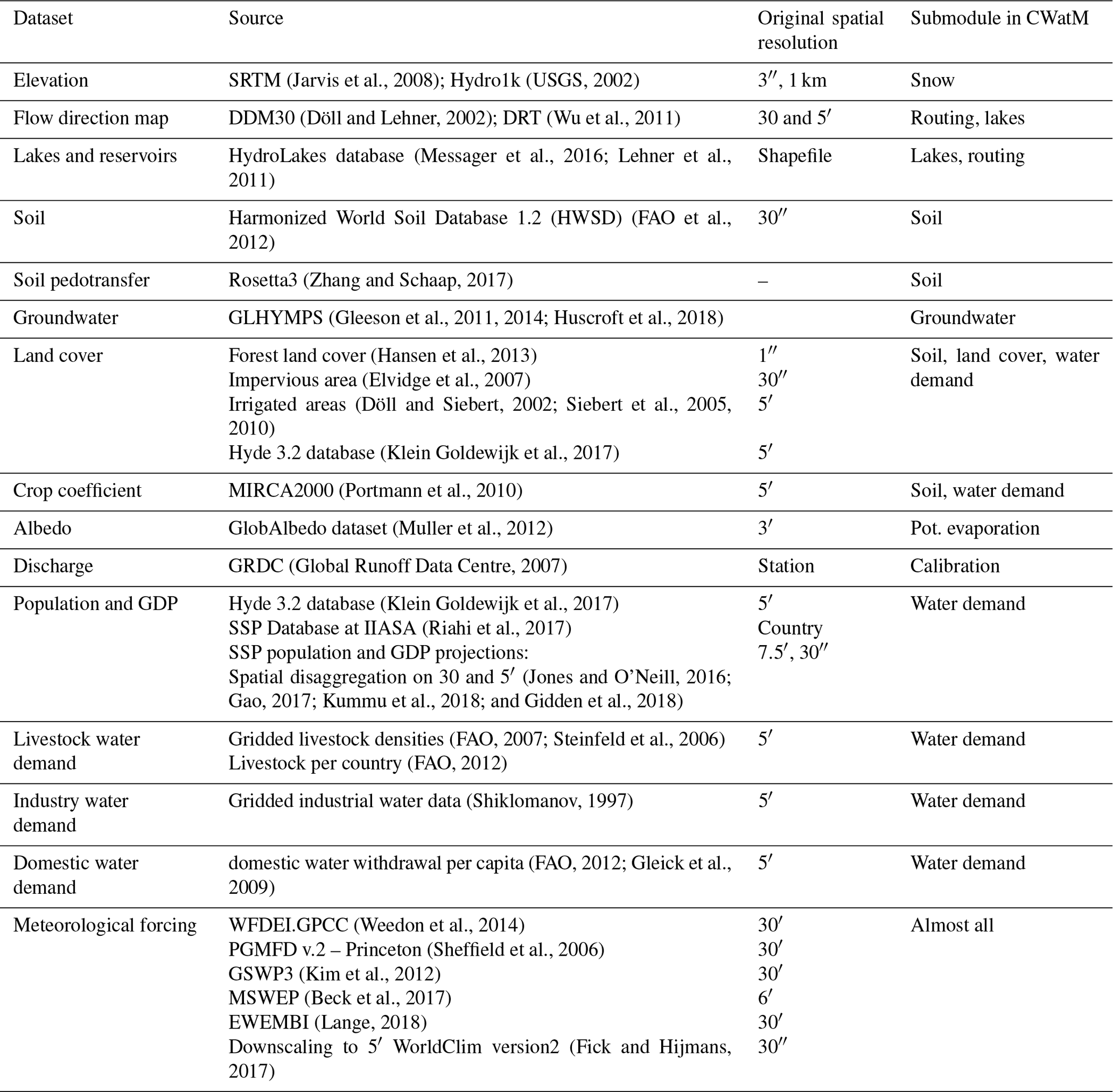
Various global datasets were used to set the framing conditions for CWatM. The model provides full global datasets for the 30 and 5′ resolutions. For both resolutions, subgrid variability is considered for certain processes; for example, for snow the subgrid variability of elevation is used, and for the effect of land cover, the subgrid variability of land use/cover in each grid cell is used. Table 1 gives an overview of the global datasets. Further descriptions of these datasets are given in the Supplement.
Table 1Global dataset, source of dataset and submodule of CWatM.
Most of the global hydrological models are uncalibrated with few exceptions, e.g., WaterGAP (Müller Schmied et al., 2014). One of the main reasons for calibrating a model is the uncertainty of its input data, parameters, model assumptions, and grid cell heterogeneity, especially at low resolution as, for example, 0.5∘ or even 5′. Samaniego et al. (2017) gives a good overview of the main challenges to improving model parametrization. Calibrating CWatM is of major importance, as the model is developed to quantify water demand versus availability for detailed regional water resources assessments that will act as the basis for interactions with stakeholders and regional policy development. For assessments of water resources and water demand and consumption such as these, realistic simulations of water resources use and availability are necessary. The main challenge of global calibration is not only the large uncertainty of input data, as well as the lack of data and validation data, but also that the hotspots of water crisis occur in data-poor regions such as Africa and parts of Asia. For CWatM, calibration uses an evolutionary computation framework in Python called DEAP (Fortin et al., 2012). DEAP implemented the evolutionary algorithm NSGA-II (Deb et al., 2002), which is used here as single objective optimization.
As objective function, we used the modified version of the Kling–Gupta efficiency (Kling et al., 2012), with r as the correlation coefficient between simulated and observed discharge (dimensionless), β as the bias ratio (dimensionless), and γ as the variability ratio.
where and , where CV is the coefficient of variation, μ is the mean streamflow (m3 s−1), and σ is the standard deviation of the streamflow (m3 s−1). KGE′, r, β, and γ have their optimum at unity. KGE′ measures the Euclidean distance from the ideal point (unity) of the Pareto front and is therefore able to provide an optimal solution which is simultaneously good for bias, flow variability, and correlation. For a discussion of the KGE objective function and its advantages over the often used Nash–Sutcliffe efficiency (NSE) or the related mean squared error, see Gupta et al. (2009) and Hrachowitz et al. (2013).
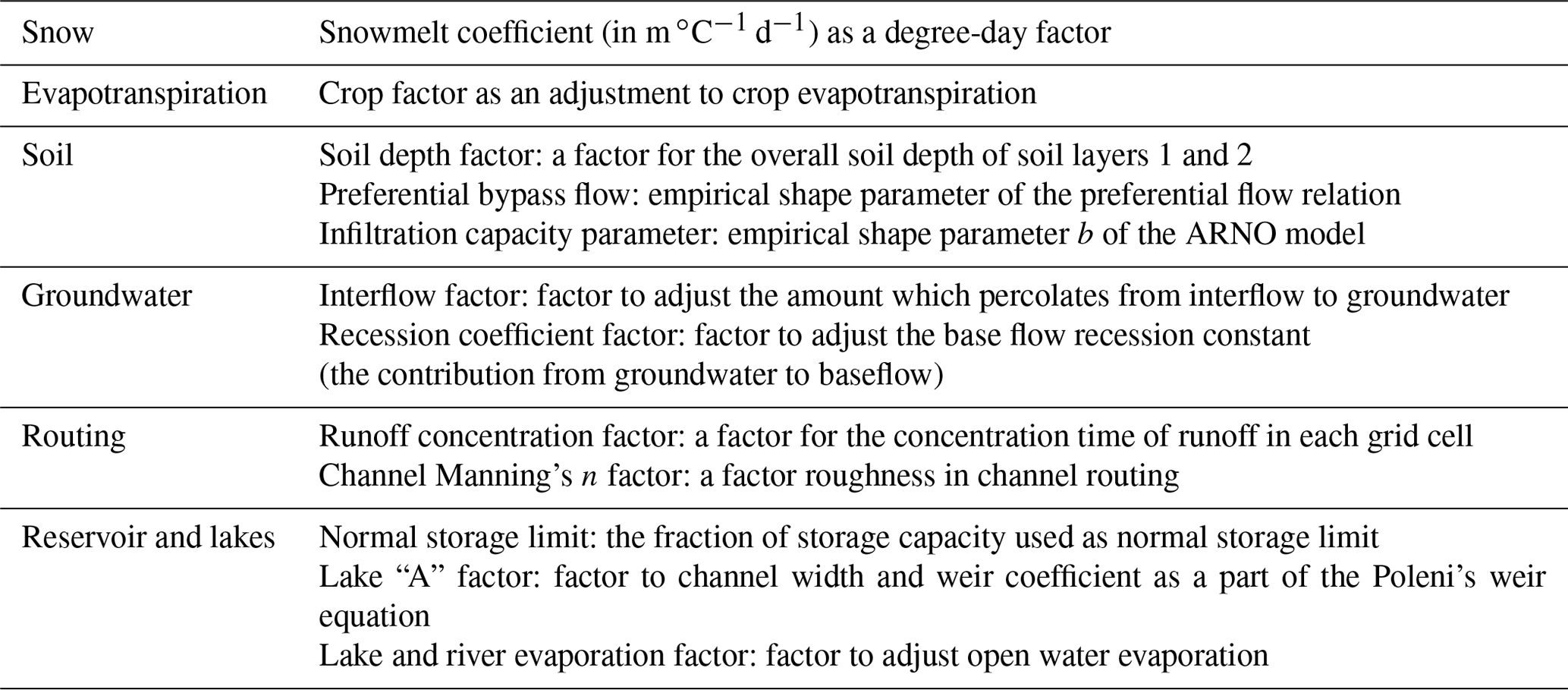
The calibration uses a general population size (μ) of 256, a recombination pool size (λ) of 32. The number of generations is set to 30, which we found to be sufficient to achieve convergence for stations. The calibration parameters are listed in Table 2. For the example of the Rhine catchment at 5′ resolution, a single simulation of 20 years (5 years as spin-up time and 15 years for comparing to observed data) takes around 40 min. After an initial 256 simulations for the general population, another 960 simulations are run (30 generation times 32 pool sizes). Altogether, these 1216 simulations are run on 32 CPU cores in parallel sessions in around 25 h.
Table 2Calibration parameters (with flexibility to adjust the number and different parameters).
5.1 Computational performance of CWatM
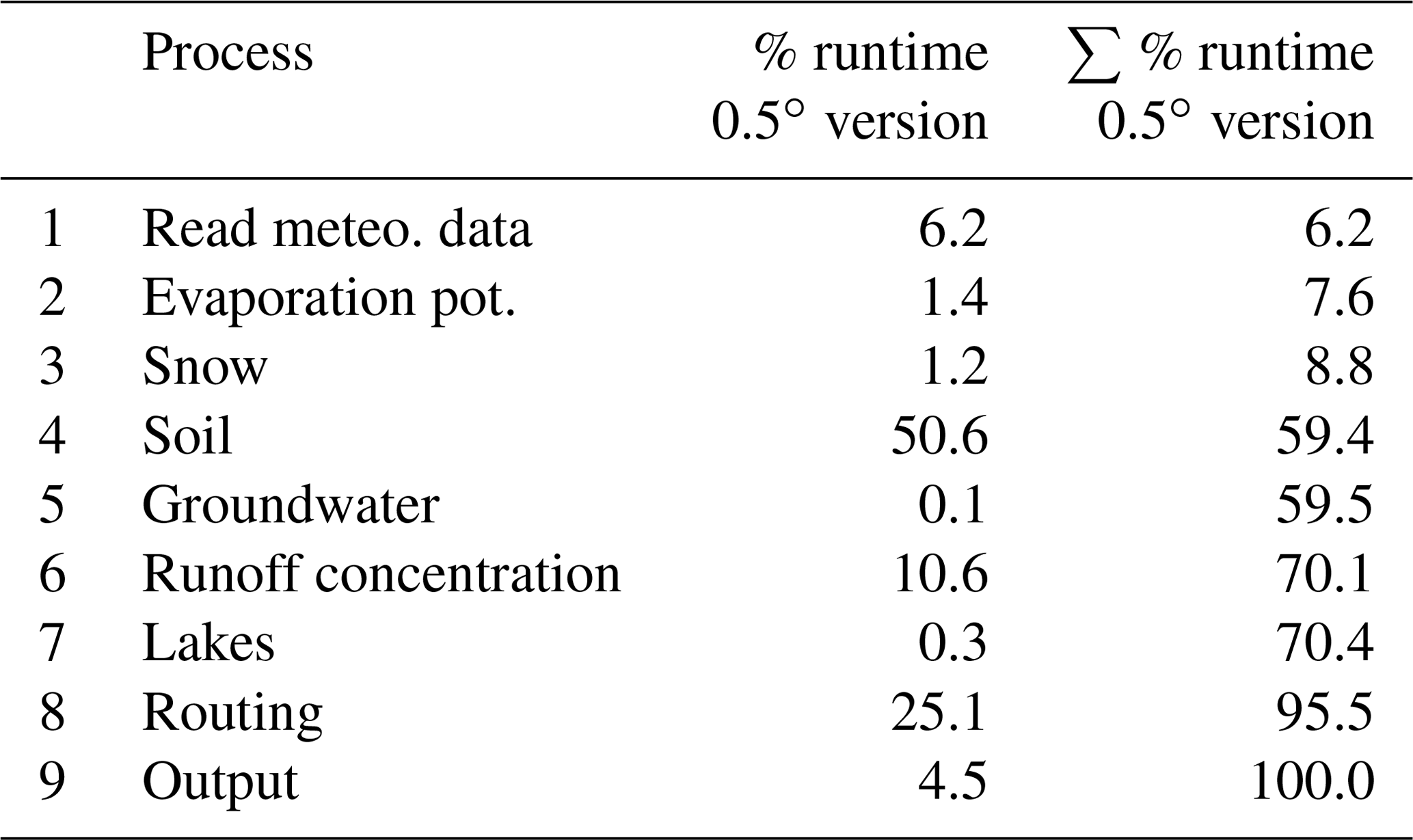
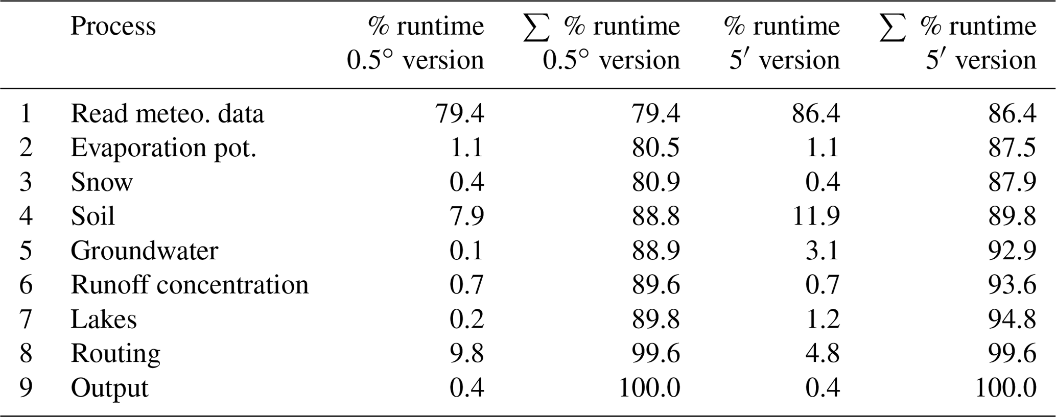
With a daily time step, a global run of 100 years takes around 12 h, i.e., 7.2 min per year (on a Linux single CPU core – 2400 MHz with Intel Xeon CPU E5-2699A). For the global setting, soil processes are the most time-consuming part, taking 50 % of all computing time, followed by routing with 25 % and runoff concentration with 10 %.
Table 3Computational time for a 0.5∘ global run in sequence of hydrological process (rain to river) and module setup.
A basin run – e.g., for the Rhine basin which is 160 800 km2 in size, using a mask map from the global dataset (netCDF map sets) – needs 40 min (0.5∘) or 3 h (5′) for 100 years, i.e., 24 s yr−1 for the 0.5∘ version and 110 s yr−1 for the 5′ version. For the Rhine basin, reading input maps takes up 79 %, which is by far the most time-consuming process, followed by 10 % for routing (kinematic wave) and 8 % for soil processes.
Table 4Computational time for 0.5∘ and 5′ runs – Rhine basin (same as Table 3).
5.2 Global water balance
The main global water balance components are calculated for the period 1979–2016 with the standard deviation of interannual variation. The spatial extent is from 90∘ N to 60∘ S. The global 0.5∘ run uses a noncalibrated global standard parameter set. The meteorological forcing uses the WFDEI data (Weedon et al., 2014). Table 5 shows the estimated global water balance components. Global average annual precipitation is around 125 000 km3 yr−1, which is 850 mm yr−1 (assuming the CRU (Climate Research Unit) land mask and the WGS84 ellipsoid). Average runoff is 51 000 km3 yr−1 and average actual evaporation is 71 700 km3 yr−1. This is in the range of other global hydrological models (Haddeland et al., 2011). The runoff fraction is 0.42, which is at the lower end compared to other models (Haddeland et al., 2011) but can be explained because CWatM takes into account evaporation from lakes and rivers. Groundwater recharge amounts to 19 000 km3 yr−1, which is higher than some of the GHMs (Mohan et al., 2018), such as WaterGAP or FAO statistics, but lower than PCR-GLOBWB2 (Sutanudjaja et al., 2018) or MATSIRO (Koirala et al., 2012). Figure 2 shows the spatial distribution of discharge and groundwater recharge which is similar to the distributions shown in Koirala et al. (2012) and Mohan et al. (2018).
Table 5Global water balance components over the period 1981–2016 simulated by CWatM.
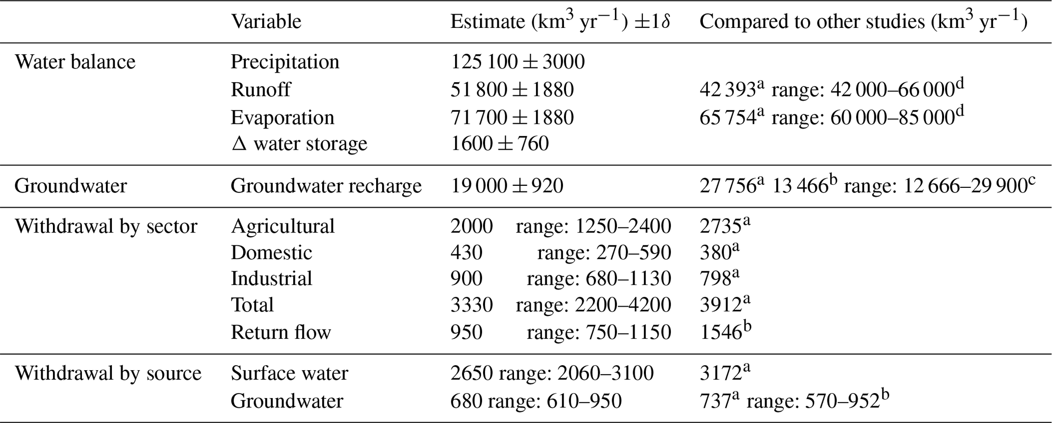
a Sutanudjaja et al. (2018), b Hanasaki et al. (2018), c Mohan et al. (2018), d Haddeland et al. (2011).
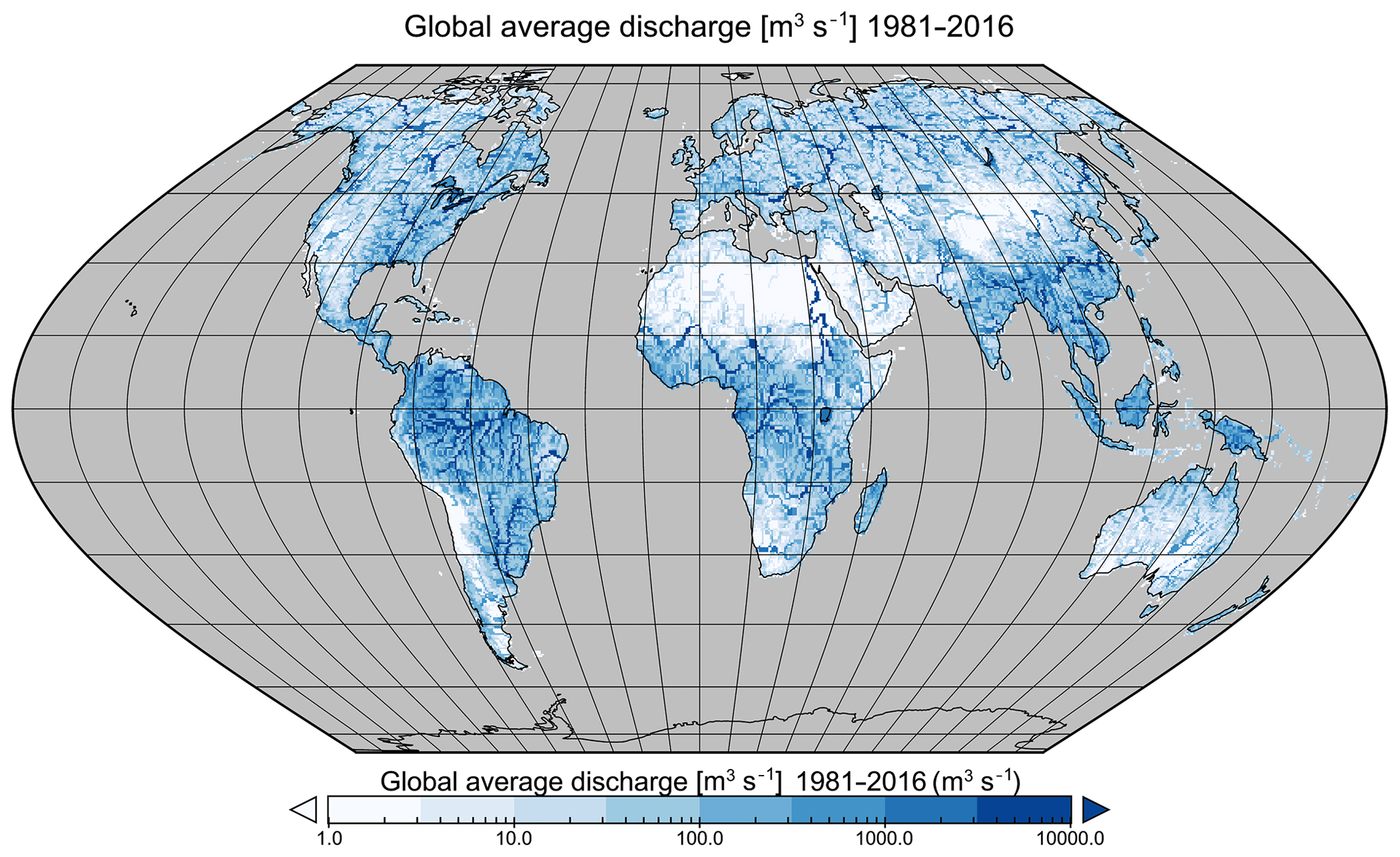
Figure 2Average global discharge (in m3 s−1, 1979–2016).
It is important to note that water withdrawals from the agricultural sector (irrigation and livestock), industry, and domestic sector (households) have been increasing over the years. The range in Table 5 for domestic and industry withdrawals has been rising constantly from 1981 to 2016. Agricultural withdrawals have been increasing over time but achieved their maxima during globally warm years, e.g., 2002, 2009, and 2012. Water withdrawal from either surface water or groundwater is within the range of other models. It has also been affected by the increasing water withdrawal for agriculture, industry, and households.
5.3 Global model validation
We used daily discharge simulations (0.5∘ resolution) for the 1971–2010 period to compare against observed discharge from the Global Runoff Data Centre (GRDC, Koblenz, Germany). Simulated discharge is based on a standard parameter set used globally before any catchment calibration shown in Sect. 5.4. Observed river discharge from GRDC includes more than 9800 (by 2019) stations worldwide with daily and monthly records of discharge. We used the approach and dataset of Zhao et al. (2017) to select a suitable set of daily discharge time series. The selection is based on (a) a minimum of 5 years coverage during the period 1971–2010; (b) a minimum catchment size of 9000 km2, to have at least three grid cells representing the basin; and (c) keeping stations with no more than 30 % difference in upstream area based on GRDC in comparison with the upstream area calculated based on the river network DDM30 (Döll and Lehner, 2002). This led to a set of 1366 stations with daily data. For every station, four performance metrics were computed by comparing daily simulated discharge with observed discharge. These include Kling–Gupta efficiency (KGE), Nash–Sutcliffe efficiency (NSE), Pearson's correlation (R), and percent bias (PBias) of mean. Table 2 shows the results of the performance metrics, and Fig. 3 shows the global distribution of the KGE. The R values ranked better than the KGE or the NSE value, and the results are in general better for Europe, South America, and the east and west coasts of North America, but there are poor results for Africa. The histograms in Fig. 4 show that a better performance is mostly apparent for larger basins. Sutanudjaja et al. (2018) showed similar results with the model PCR-GLOBWB and explained the lack of performance partly with the poor performance of meteorological forcing. A better explanation of performance differences in global hydrological models will be given by the ISI-MIP (Warszawski et al., 2014) model intercomparison where CWatM is part of the ISIMIP2bmodel consortium.
Table 6Performance metrics based on 1366 GRDC stations.
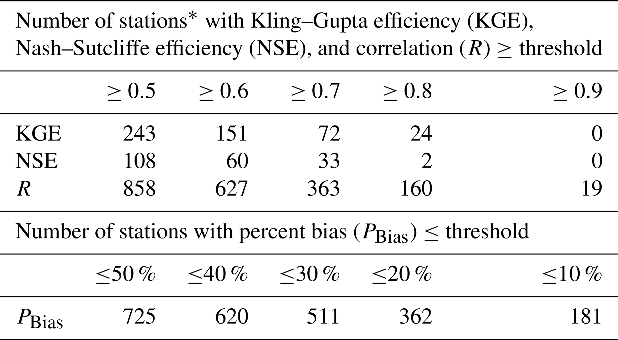
* based on sample size of 1366 GRDC stations
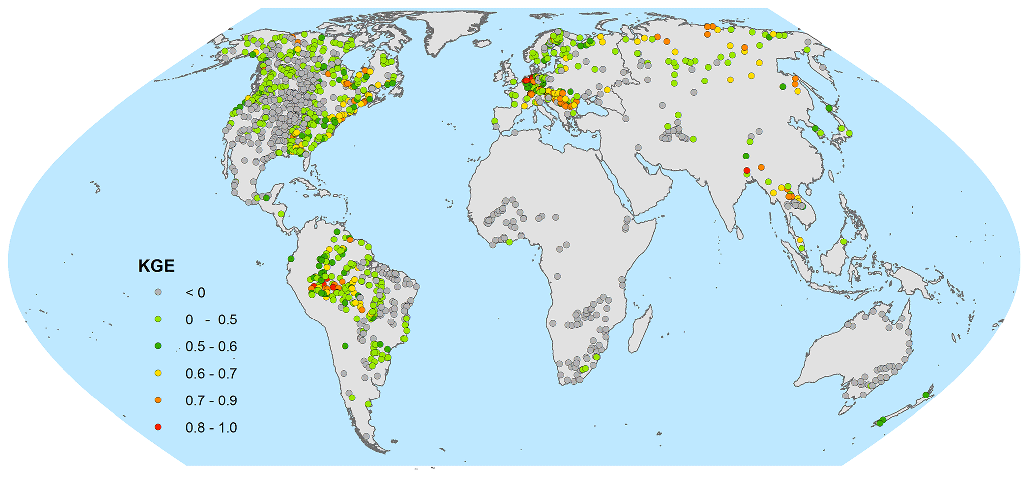
Figure 3Global map of Kling–Gupta efficiency based on 1366 GRDC stations.
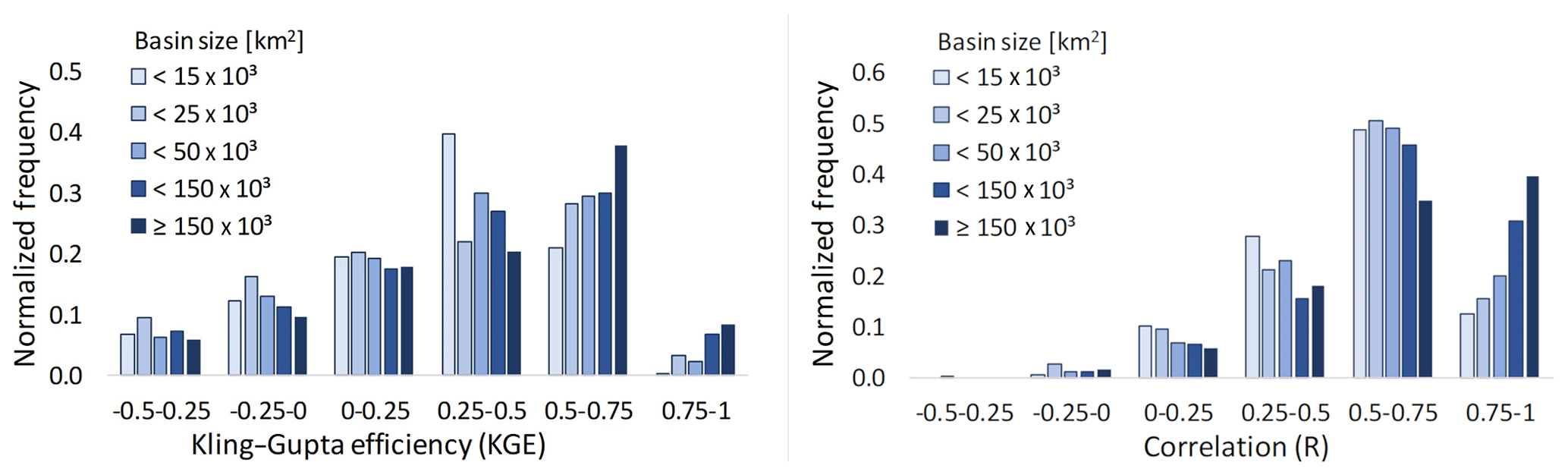
Figure 4Histograms of Kling–Gupta efficiency and correlation for different basin sizes based on 1366 GRDC stations.
Some model papers (e.g., Döll et al., 2014; and Sutanudjaja et al., 2018) use observed discharge stations or the Gravity Recovery and Climate Experiment (GRACE) (Tapley et al., 2004) to evaluate the global results of their models. As CWatM is a part of the ISIMIP intercomparison project, we think it is best to show the performance of a model in the framework of ISIMIP by comparing it to other models like in Zhang et al. (2017) or Scanlon et al. (2018). An upcoming paper by Pokhrel (2020) on global terrestrial water storage will include a comparison of seven global terrestrial hydrology models (including CWatM) against GRACE data.
5.4 Global calibration results
For calibration, an evolutionary algorithm with KGE as objective function was applied and WFDEI meteorological data were used as forcing. For all stations, the calibration improved the streamflow simulations compared to the baseline simulation with a default parameter set. During the calibration, human activities (e.g., water abstraction, reservoirs, and changing land cover of time) are included. However, the performance varied depending on the quality of the discharge data and the meteorological forcing, as well as on the processes included in CWatM, as shown in Table 7. Calibration and validation results are shown for each station in the Supplement part 3. Simulating processes such as backflow or large evaporation losses due to swamps in the Nile and Niger basin are still challenging. But this simulation shows the suitability of CWatM for representing the major water balance components and the necessity of calibrating certain basins, especially where water availability is being compared with water withdrawal. A further step in global calibration must be performed by regionalization of model parameters, e.g., by using model parameters from well-performing basins for basins with similar climate and other characteristics (Samaniego et al., 2010, 2017; Beck et al., 2016). A big challenge is the unevenly distributed observed discharge data around the world with big spatial gaps in Africa and Asia. Even if calibration with an objective function based on observed discharge is the best option, the gap might be filled with some sort of Budyko calibration (Greve et al., 2016), where at least the empirical function of actual evapotranspiration against potential evaporation is fitted or satellite-based river levels could replace discharge missing from the observations (Revilla-Romero et al., 2015; Gleason et al., 2018).
Table 7Calibration results for some catchments worldwide.
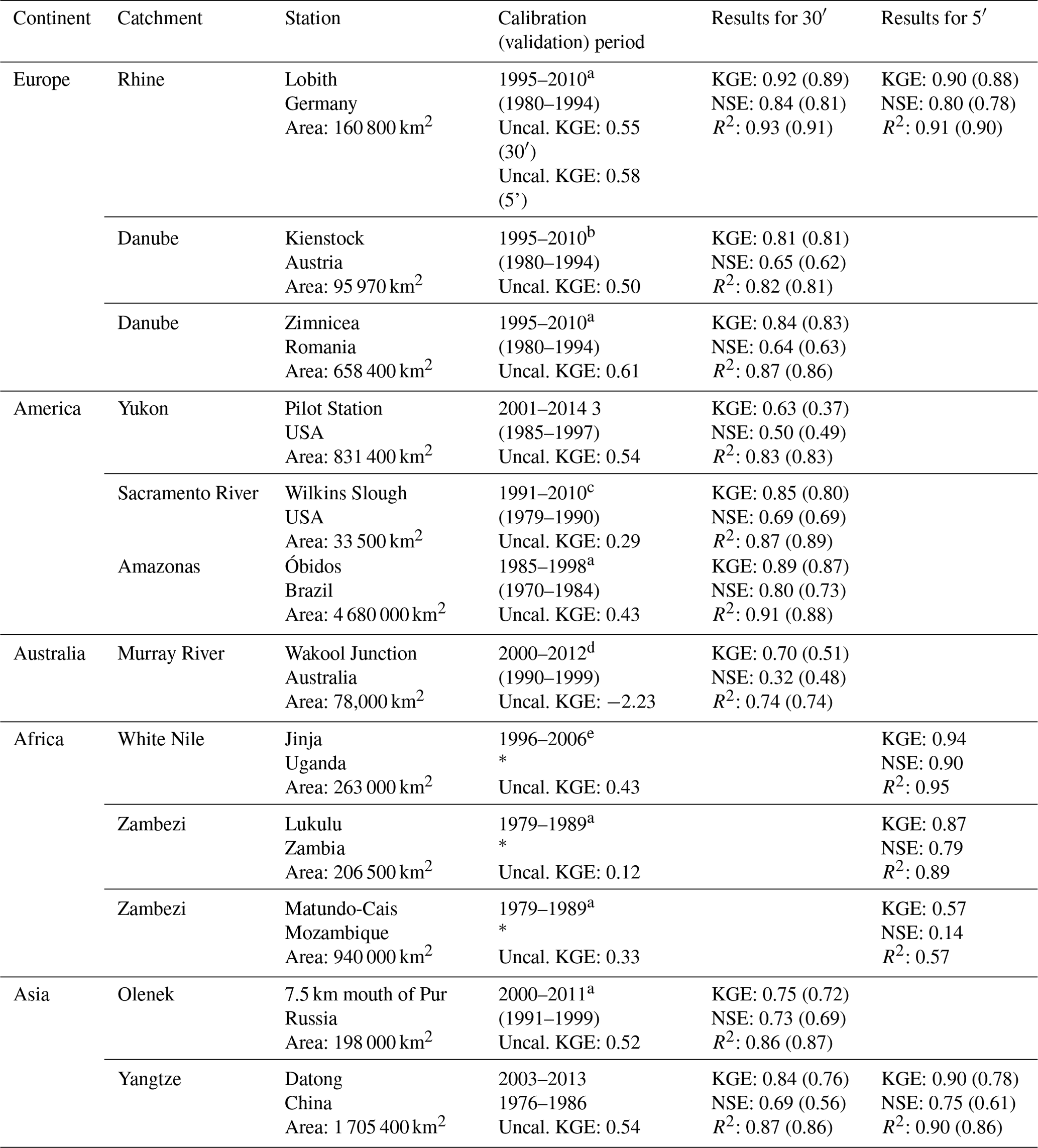
* All observed data used for calibration period. Data for calibrating discharge are from a GRDC, Global Runoff Data Centre, https://www.bafg.de/GRDC (last access: 27 June 2020); b viadonau, viadonau Österreichische Wasserstrassen-Gesellschaft, http://www.viadonau.org (last access: 27 June 2020); c USGS, United States Geological Survey, https://www.usgs.gov (last access: 27 June 2020); d MDBA, Murray–Darling Basin Authority, https://riverdata.mdba.gov.au (last access: 27 June 2020); and e Ministry for Water and Environment, Uganda, https://www.mwe.go.ug (last access: 27 June 2020).
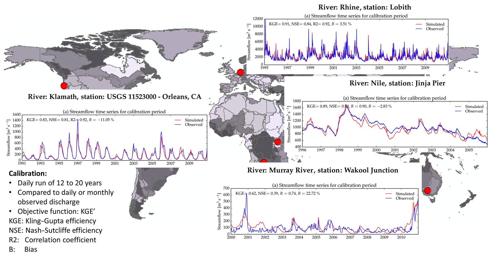
Figure 5Calibration results for some chosen stations globally.
5.5 Regional water balance: example of East Africa
5.5.1 The extended Lake Victoria basin
The essential component of the Water Futures and Solution Initiative of IIASA (Burek et al., 2016; Wada et al., 2016) is the assessment of the balance of water supply and demand for the present and into the future. With the support of the Government of Austria through the Austrian Development Agency (ADA), we aim to provide a deeper understanding of critical parameters for achieving water security in East Africa. This is in the context of competing demands for basic water supply, sanitation, food security, economic development, and the environment. UN-Water (2013, p. 1) defines water security as the following:
The capacity of a population to safeguard sustainable access to adequate quantities of and acceptable quality water for sustaining livelihoods, human well-being, and socio-economic development, for ensuring protection against waterborne pollution and water-related disasters, and for preserving ecosystems in a climate of peace and political stability.
Water security is also a key ambition expressed in the “Vision 2050” of the East African Community (EAC, 2016) as rapid growth of the economy and population and a high rate of urbanization are expected for the region and will lead to increased water demand in all sectors as well as further pressure on the water quality status.
The examples of operational areas for CWatM in this paper are not presented with specific results in mind, nor do they reflect results from the project's intensive stakeholder processes. They are there to demonstrate the value of a global hydrological model used in a regional case study that combines the spatiotemporal scale dependencies of water systems produced through a scenario analysis designed to include both the regional and global scales. An “East Africa Regional Vision Scenario” (EA-RVS) was developed (Tramberend et al., 2019, 2020), based on regional visions, and we used available regional scenarios and data that were developed in the context of global studies. As well as regional visions, the study also integrates into the widely applied global scenario development process of the Intergovernmental Panel on Climate Change (IPCC). It is characterized by a Scenario Matrix Architecture (van Vuuren et al., 2014) including the community-developed Shared Socioeconomic Pathways (SSPs) (Jiang and O'Neill, 2017) and the Representative Concentration Pathways (RCPs) (van Vuuren et al., 2011) for the characterization of climate change.
The study area, the extended Lake Victoria basin (eLVB), is a transboundary basin in the tropics. It comprises the headwaters of the Nile and includes an area of over 460 000 km2. The Equator crosses the region approximately in the middle of the eLVB just south of Kampala. The eLVB includes the source of the Nile and major lakes in East Africa, foremost Lake Victoria, Lake Albert, Lake Edward, and Lake Kyoga. The eLVB has been subdivided into interconnected subbasins. According to the water flow regime, we have aggregated the 61 basins into eight major basins (see Fig. 6). The CWatM model setup uses the default global dataset at 5 arcmin. Discharge data for calibrating river discharge were made available courtesy of the Ministry of Water and Environment, Uganda. Calibration is performed for three stations. The calibration parameters are valid for the subbasin up to the gauging station. The upstream station is calibrated using the best fit of the downstream calibrated subbasins. The 10 years of available observed data are used for the calibration period. Therefore, no other time period is available for a validation period.

Figure 6The 61 subbasins of the eLVB and their aggregation into eight major basin regions.
5.5.2 Seasonal pattern of the discharge regime
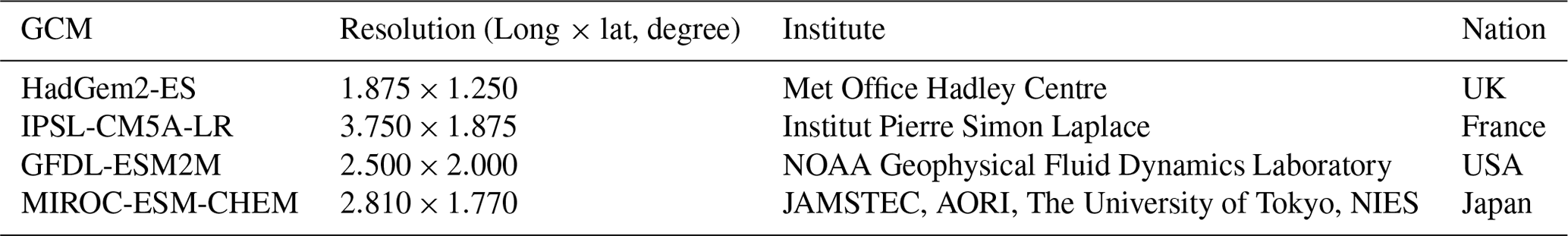
For assessing climate change impact, RCP6.0 was chosen as the most plausible future for East Africa by the “EAC Vision 2050” (EAC, 2016) even though it represents a rather pessimistic outlook of global temperature increases despite being published after the Paris Climate Agreement of 2015. We have chosen the two general circulation models (GCMs) of HadGEM2-ES and MIROC5 out of the four GCMs (see Table 8) used in ISIMIP 2b (Frieler et al., 2016) as being the most feasible for eLVB as the discharge results that were run with CWatM for the historical runs of the GCMs GFDL-ESM2M and IPSL-CM5A-LR showed a large discrepancy from historical results.
Discharge is the variable which incorporates all the meteorological and hydrological processes into a basin and encompasses all the storage components in a basin (i.e., soil, groundwater, lakes, and reservoirs) Especially with the large lakes in the basin, discharge in eLVB has a long memory of past conditions.
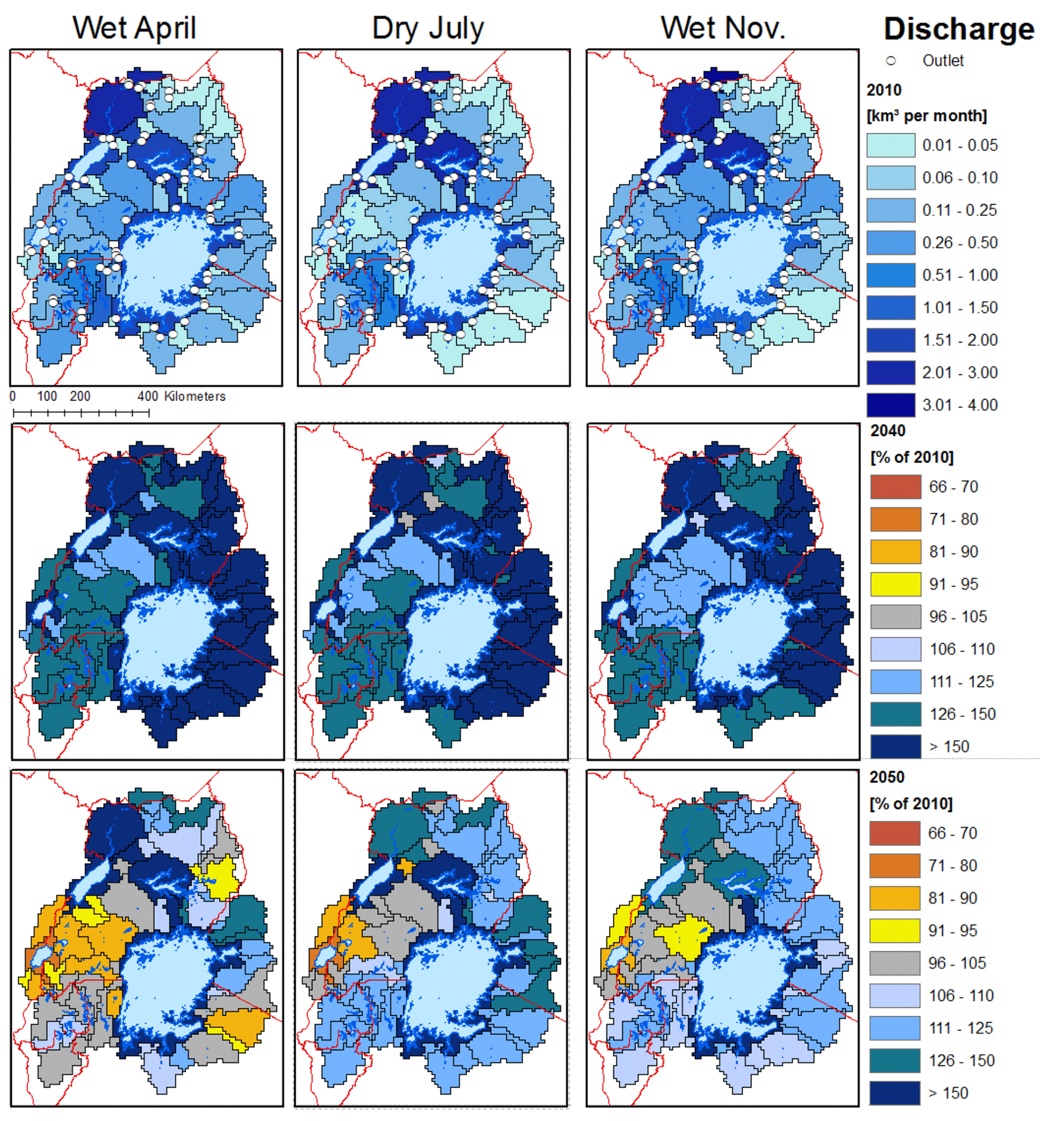
Figure 7Change of seasonal discharge pattern from 2010 to 2040 and for 2050.
The seasonal pattern of discharge in Fig. 7 shows more discharge for 2040 (10-year period 2036–2045) and 2050 (10-year period 2046–2055) in the river system from Lake Victoria, especially for the 2040 period. This is due to a wetter period of weather in the two GCMs from 2038 to 2049 and the strong memory effect of groundwater and the lakes. It also shows the big influence of interannual variability in the eLVB. Even if a general trend of less runoff in the 2050 period can be detected, long-lasting periods of wetter conditions can nevertheless be superimposed over this trend. Because of the strong interannual variability in the lower latitudes, it is difficult to assess the effect of a general climate change impact towards a wetter or drier climate. But under climate change, southwestern Uganda will show generally drier conditions than the western part of the eLVB.
5.5.3 Water scarcity indicators
Available water resources per capita, the Water Crowding Index (WCI) (also called the Falkenmark indicator), is one of the most widely used measures of water stress (Falkenmark et al., 1989). Based on per capita water availability, the water conditions in an area can be categorized into different categories of stress expressed as cubic meters (m3) of water available per capita and per year. Another indicator is the Water Resources Vulnerability Index (Raskin et al., 1997) that is also known as Water Exploitation Index (WEI) (EEA, 2005), defined as the ratio of total annual withdrawals for human use to total available renewable surface water resources. Regions are considered water scarce if annual withdrawals exceed the percentage of annual supply (Alcamo et al., 2003). The thresholds for both indicators are shown in Table 9.
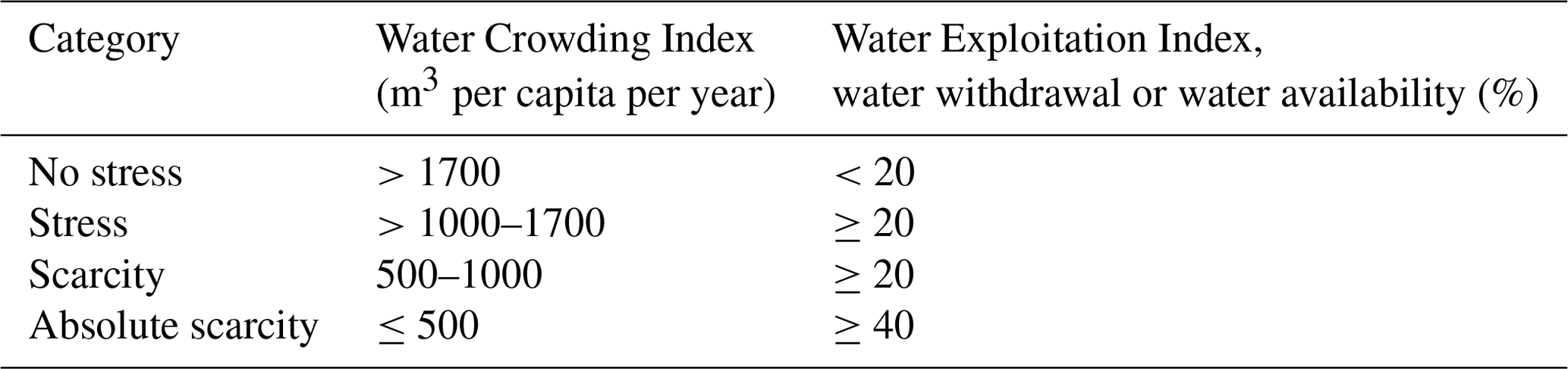
The WCI and WEI are mainly shown as annual indicators, but in regions with high intra-annual variability the rainy seasons show a different picture from that of the dry season. An example in Fig. 8 shows the WCI and WEI for the dry season and the most water-scarce month, July, for 61 subbasins of the extended Lake Victoria basin by comparing the situations of 2010 and 2050. The figure shows that there is a clear increase in the WCI. While in the current situation (2010) about half of the subbasins are exposed to some level of water scarcity with some subbasins indicating absolute water scarcity, in 2050 almost all subbasins that are neither directly crossed by the river Nile nor adjacent to a lake experience stress or scarcity and many of them absolute water stress. The water resource availability for the WEI is also based on the RCP6.0 climate scenario and includes the effect of human consumption and effects of land use change up to 2050. Looking at this index for the month of July only, it shows that 9 out of 61 subbasins are likely to experience water scarcity and even severely water-scarce situations by 2050. Such subbasins are mainly located at the south and southeastern shores of Lake Victoria and in densely populated areas of Rwanda and Burundi.
Interestingly, the WEI shows a much lower signal of water scarcity compared to the WCI. The WCI assumes that, regardless of the socioeconomic conditions, every person on the globe has the same “water demand entitlement”. The Water Exploitation Index is based on the in situ situation and on balancing changing water availability and water demand. The fact that both indices show a rather different picture might be interpreted as an indication of economic water scarcity. The situation of low economic development for the extended Lake Victoria basin may still prevail in 2050 (at least compared to the global average). This is the main reason for the relatively low actual water demand compared to global averages and therefore relatively low water scarcity signal for the WEI compared to the WCI.
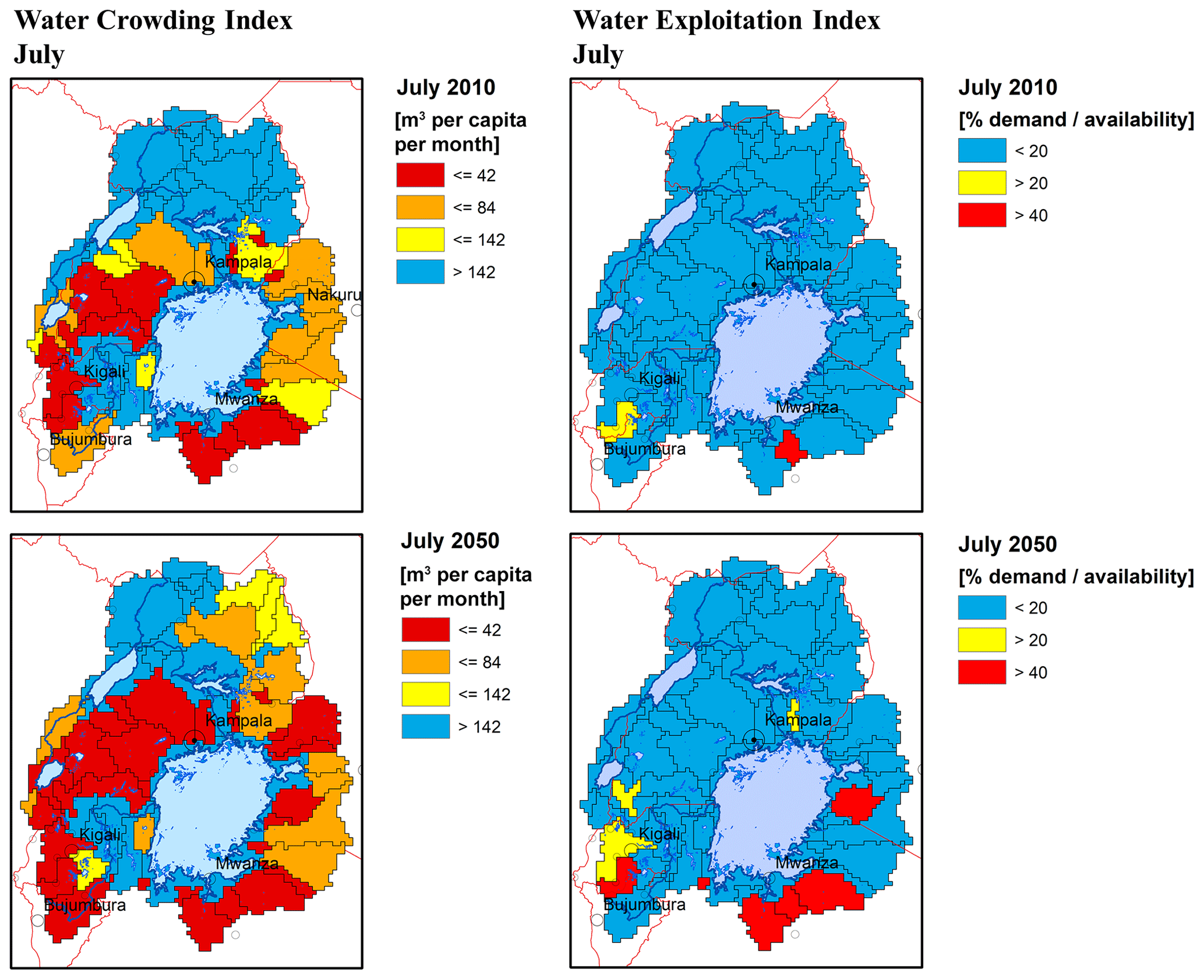
Figure 8Water Crowding Index and Water Exploitation Index in July for the extended Lake Victoria basin.
5.6 Regional water balance: example of the Zambezi
5.6.1 Calibration and comparison with other GHMs
The hydrological model CWatM is intended to be scalable and can be applied over finer spatial scales (e.g., the basin). CWatM has been calibrated for the Zambezi, using six subcatchments and measured discharge provided by the Global Runoff Data Centre (2007). Figure 9 shows two time series of measured vs. simulated river discharge, and the comparison shows good agreement of the modeled discharge with the measured data. The station Matundo-Cais is downstream of the two big reservoirs Kariba Dam and Cahora Bassa, which are included in the model. The reservoir operations are calculated with the approach in Sect. 2.3.11.
By comparing the outputs of the hydrological model ensemble, we see that, especially for sub-Saharan Africa, there is a strong overestimation of river discharge, which indicates an erroneous picture if compared, for example, to water demands for calculating water scarcity. Figure 10 shows a comparison of discharge for the Lukulu in the Zambezi basin of different hydrological models as a violin plot which shows the probability density of the data. While a box plot shows some statistics like mean and quartiles a violin plot shows the full distribution of the data.
The GHMs in Fig. 10 use the WFDEI (Weedon et al., 2014) as forcing meteorological data from 1981 to 2004. Apart from WaterGAP and CWatM (both calibrated), one can see a strong overestimation of discharge for all other models compared to the observed discharge and some models also show a different shape than the observed data.

Figure 9Calibration results for two stations in the Zambezi basin.
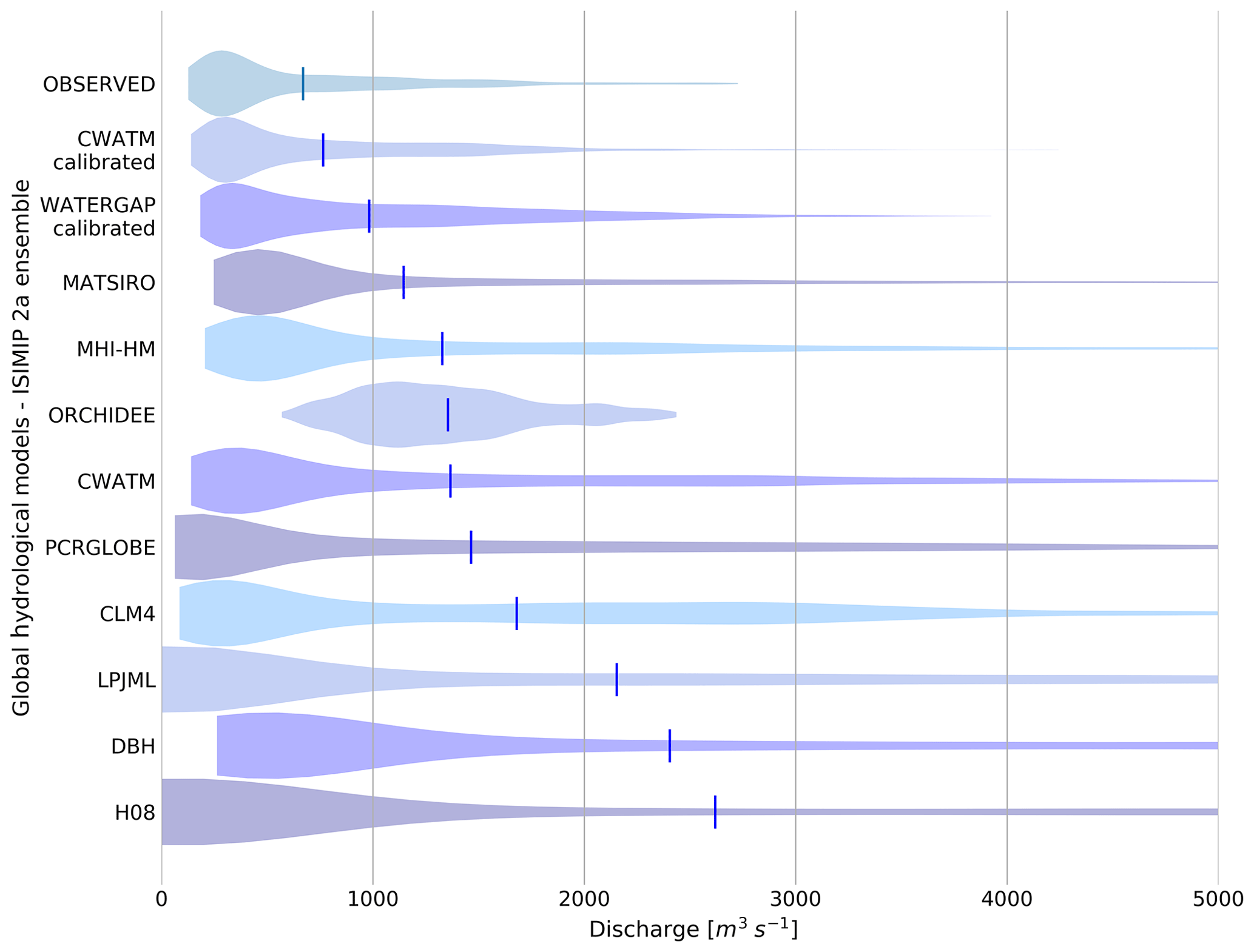
Figure 10Discharge for Lukulu/Zambezi from 1981 to 2004 for 11 different global hydrological models from the ISIMIP 2a ensemble compared with observed discharge. Each violin plot shows the probability density of the data for the different GHMs. The lines show the average discharge for each model.
Average discharge is overestimated for the noncalibrated models from 2 up to 3 times and maximum discharge up to 7 times. This shows the need to put efforts into calibration of the hydrological model for regional applications to be in line with measured water resources and to minimize the uncertainty from hydrological modeling. Setting up model calibration has been time-consuming but inevitable for the Zambezi case study.
Calibration for the Zambezi basin is performed for six stations (Lukulu, Kongola, Katima, Kafue Hook, Luangwa Road Bridge, Tete – see Fig. 6). The calibration parameters are valid for the subbasin up to the gauging station. The upstream station is calibrated using the best fit of the downstream calibrated subbasins. The parameter set is valid for the subbasin except for the downstream subbasins which have their own parameter sets.
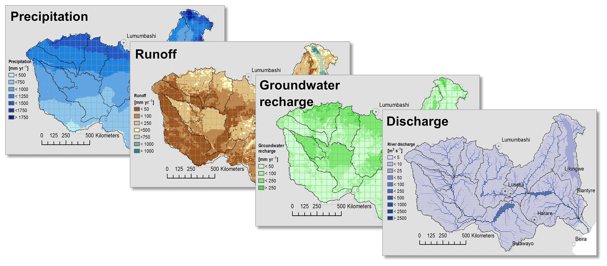
Figure 11Parameter sets of different hydrological variables.
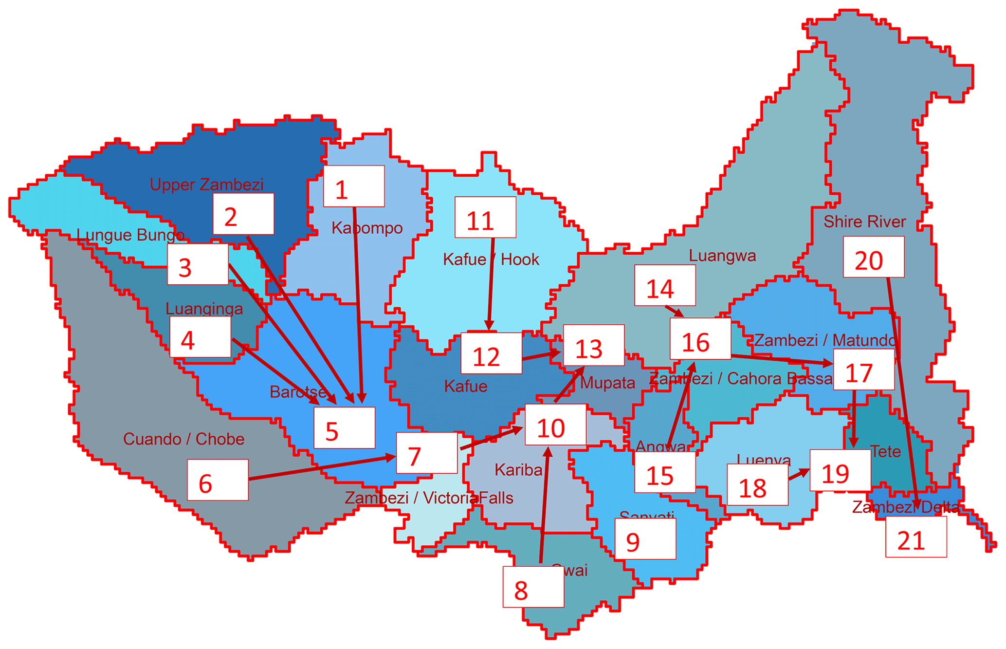
Figure 12Subbasins of the Zambezi basin for aggregating data from CWatM.
5.6.2 Assessment of water stress
In a second phase, the CWatM calibrated model is used to assess water scarcity until 2050 in the Zambezi basin. Water resources at each grid cell are dependent on climate; water management (e.g., reservoirs); and water use for irrigation, livestock, domestic, or industry. For each cell (at 5′) (see Fig. 11) and for aggregated regions, water resources can be related to water demand from different sectors. Results from the distributed hydrological model CWatM are aggregated into 21 subbasins (see Fig. 12) based on a regional distribution shared by the Zambezi Water Commission (http://zamwis.wris.info, last access: 27 June 2020). In addition, the regions of Kariba, Kafue, and Tete are split into, respectively, four, two, and four subbasins to look specifically into the more densely populated areas.
Projection of future water resources builds on quantifications of climate scenarios CMIP5 (Distributed by the Coupled Model Intercomparison Project (CMIP); see https://pcmdi.llnl.gov/index.html, last access: 27 June 2020) based on the RCPs from the Inter-Sectoral Impact Model Intercomparison Project (ISI-MIP) (Frieler et al., 2016). We applied climate change projections from four GCMs (see Table 8) for a first setting of RCP6.0. Land use data projection is used from the GLOBIOM model (Havlík et al., 2013). Nineteen different crop types with different classes of farming intensity and eight land use classes (e.g., forest, build up classes) of GLOBIOM output, for different RCPs and SSPs, are transformed to fit into the arrangement of six land use classes of CWatM.
Water demand for agriculture is taken from calculations within CWatM. Water demand for domestic, livestock, and industry is calculated within CWatM using the approach of Wada et al. (2011). The socioeconomic background needed for this approach uses data and methods for spatial disaggregation for the SSP2 scenario from Jones and O'Neill (2016), Gao (2017), Klein Goldewijk et al. (2017), Kummu et al. (2018), and Gidden et al. (2018).
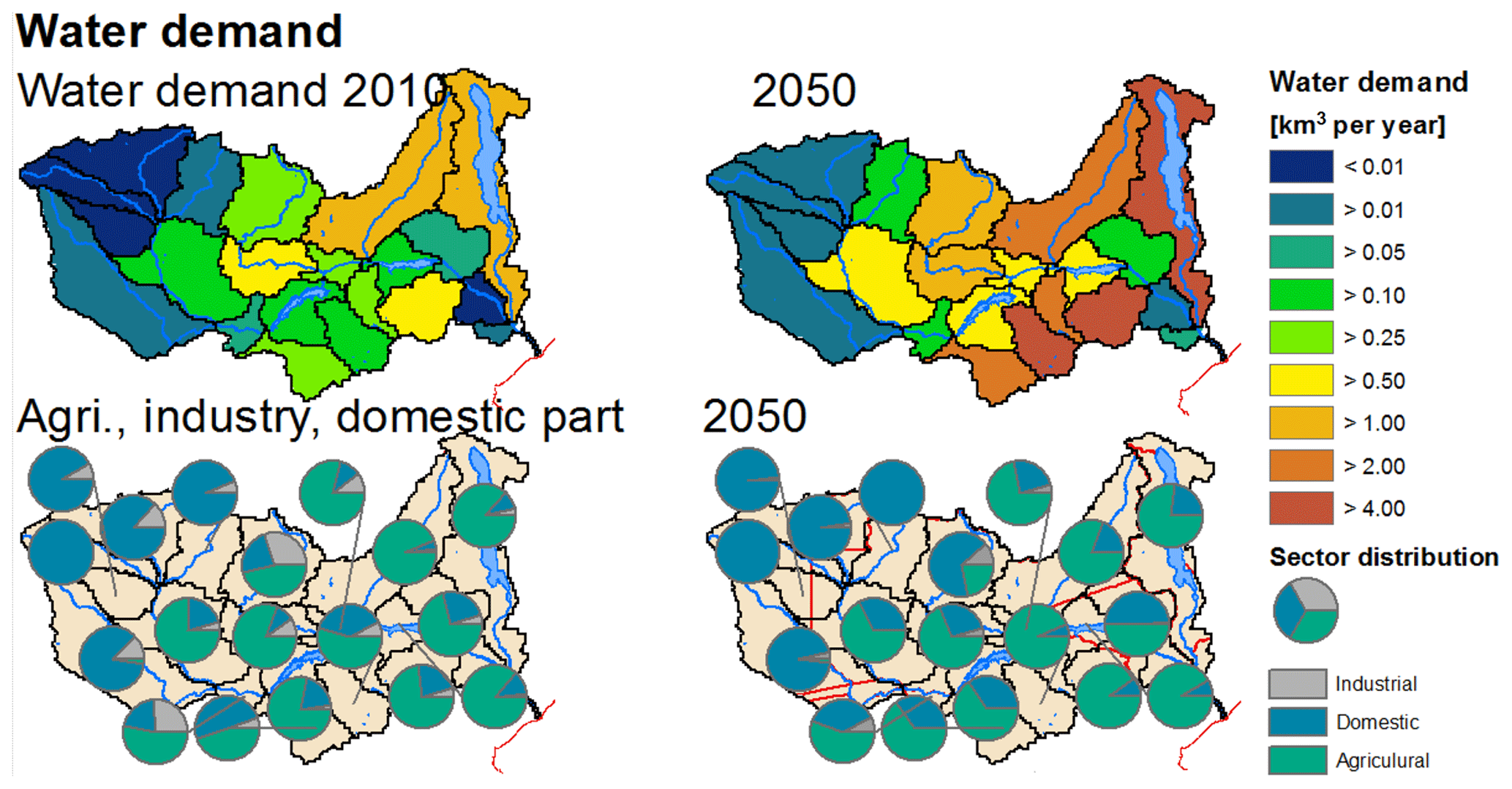
Figure 13Water demand projection for scenario SSP2/RCP6.0 to 2050 based on population, GDP, and irrigation area projections.
Water Exploitation Index for Zambezi
The WEI is defined in Falkenmark et al. (1989), Falkenmark (1997), and Wada et al. (2011) as comparing blue water availability with net total water demand. A region is considered “severely water stressed” if the WEI exceeds 40 % (Alcamo et al., 2003). The yearly WEI in Fig. 12 shows no water stress for the whole basin in 2010, but water stress will intensify up to 2050 for the business-as-usual (BAU) scenario (composed of the SSP2 and RCP6.0 scenarios), mainly due to agricultural and domestic water demand increasing by a factor of 5; as annual mean river discharge is only increasing by 6 %. August is chosen for monthly comparison as this is the month with the highest rate of water withdrawal (WW) and a mean monthly discharge (MMD) that is only slightly higher than in November. The eastern part of the Zambezi basin, except for the main course of the Zambezi river, was already showing severe water stress in 2010. This will increase in 2050, but the western part is still not suffering from water stress.
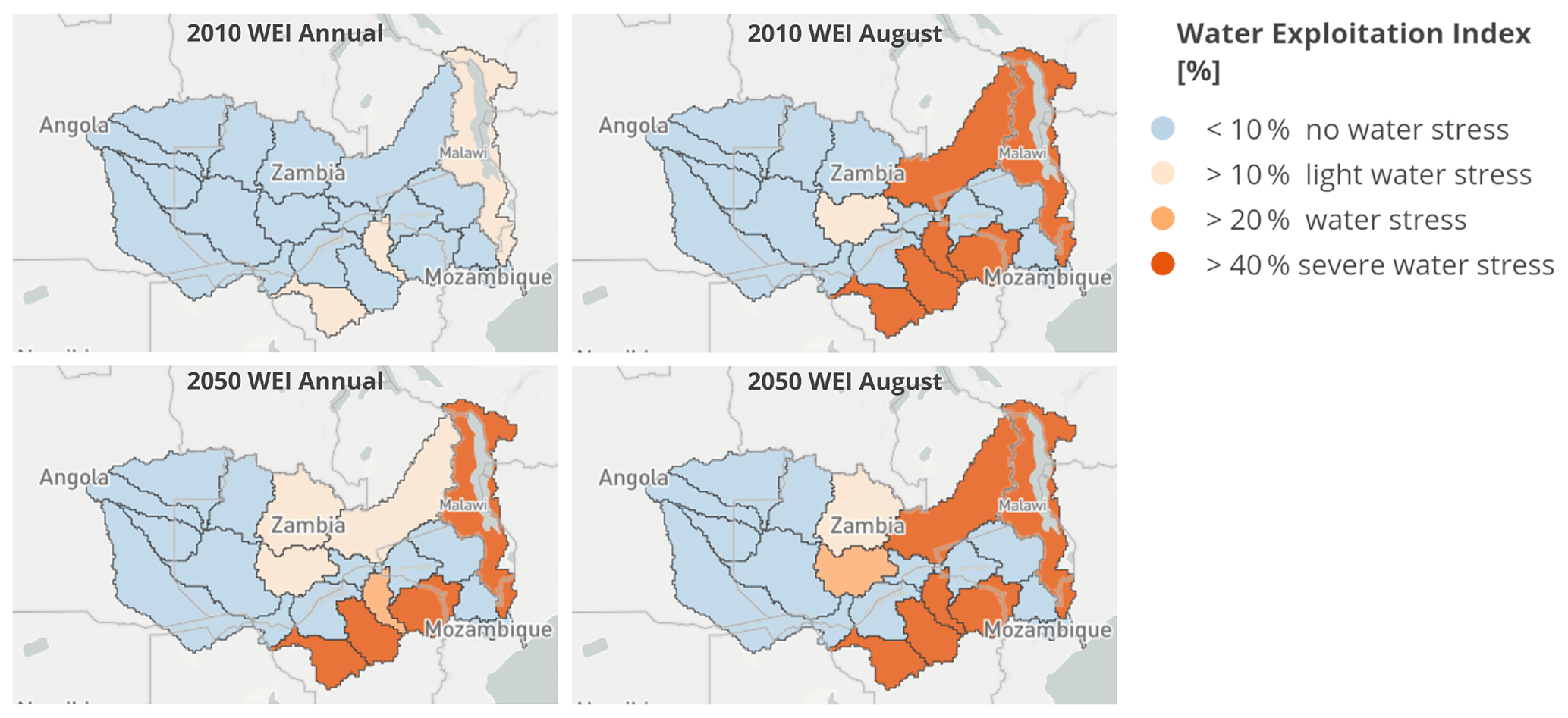
Figure 14Water Exploitation Index for 21 regions of the Zambezi for 2010 and 2050 using the business-as-usual (BAU) scenario (yearly and for the month of August).
The modular structure of CWatM helps to link and integrate with other models. The independent settings files offer possibilities to adapt the input and output to other models. For a lot of applications, no intervention into the code is necessary. If code has to be customized to the linked model, the modular structure of CWatM easily allows users to identify the point of intervention.
To explore potential sustainable pathways for the Zambezi basin, an integrated assessment framework is needed. Therefore CWatM provides data on water availability (runoff and discharge) and water demand (irrigation, domestic, and industrial demands) at subbasin level to the “Extended Continental-scale Hydroeconomic Optimization” (ECHO) model (Kahil et al., 2018) and to the water quality model “Model to Assess River Inputs of Nutrients to seas” (MARINA) (Strokal et al., 2016). Figure 15 gives an overview of the interactions between models and the data flow.
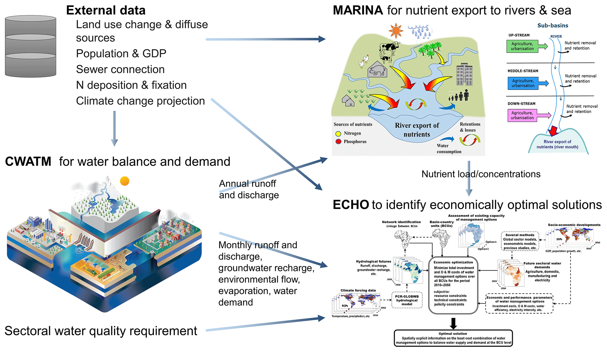
ECHO is a hydro-economic optimization model. Its objective function minimizes the costs of water management options subject to several resource and management constraints across subbasins within river basins over a long-term planning horizon (e.g., a decade or more). ECHO includes a wide range of supply- and demand-side water management options spanning over the water, energy, and agricultural systems. The supply options are surface water diversion, groundwater pumping, desalination, and wastewater recycling technologies. Other supply options considered in ECHO are surface water reservoirs and interbasin transfer infrastructure. The water demand management options consist of different technologies for irrigation (flood, sprinkler, and drip) and several measures to improve crop water management in irrigation and water use efficiency in the domestic and industrial sectors (Kahil et al., 2018, 2019).
To assess the impacts of human activities on water quality, the MARINA model (Strokal et al., 2016) is used to estimate nitrogen loads and concentrations. MARINA quantifies nutrient (nitrogen and phosphorus) export to rivers and sea at the subbasin scale. It is primarily used for long-term trend analysis and for source attribution, which could guide the identification of effective policy and management measures to reduce water pollution.
Moreover, MARINA uses data from GLOBIOM (Havlík et al., 2013) for land use and agricultural nitrogen inputs to the basin and socioeconomic projections (population and GDP) to estimate nitrogen inputs from human waste. ECHO uses information on existing capacities of various water management options and the costs of investment and operation of these options. Nitrogen loads and concentrations calculated by MARINA are compared with nitrogen standards for different sectors to categorize the suitability of water use by different users, which can be further used by ECHO to optimize water allocation and explore economically optimal management options. The source attribution at the subbasin scale by MARINA (Fig. 15) provides prior information for ECHO to prioritize the most relevant nitrogen management options for each subbasin, such as sewer connections, wastewater treatment, and manure and mineral fertilizer use in agriculture. Lastly, the coupling of MARINA and ECHO with CWatM enables analysis of the impacts of climate change and variability on nutrient export, water allocation, and adaptation costs. CWatM outputs from different climate forcing could be used in MARINA and ECHO to investigate the impacts of intrabasin spatial variability and interannual temporal variability of runoff and discharge. Figure 16 is an example of MARINA output of total dissolved nitrogen (TDN, in kg km−2 yr−1) for the Zambezi river basin. It illustrates the increase in river export of TDN to the sea between 2010 and 2050 (BAU scenario), the increasing share of anthropogenic nitrogen sources, and high spatial variability in the Zambezi basin (Tang et al., 2019). Another example of data exchange between CWatM and MARINA is given in Wang et al. (2019a) for Lake Taihu in the Yangtze basin.
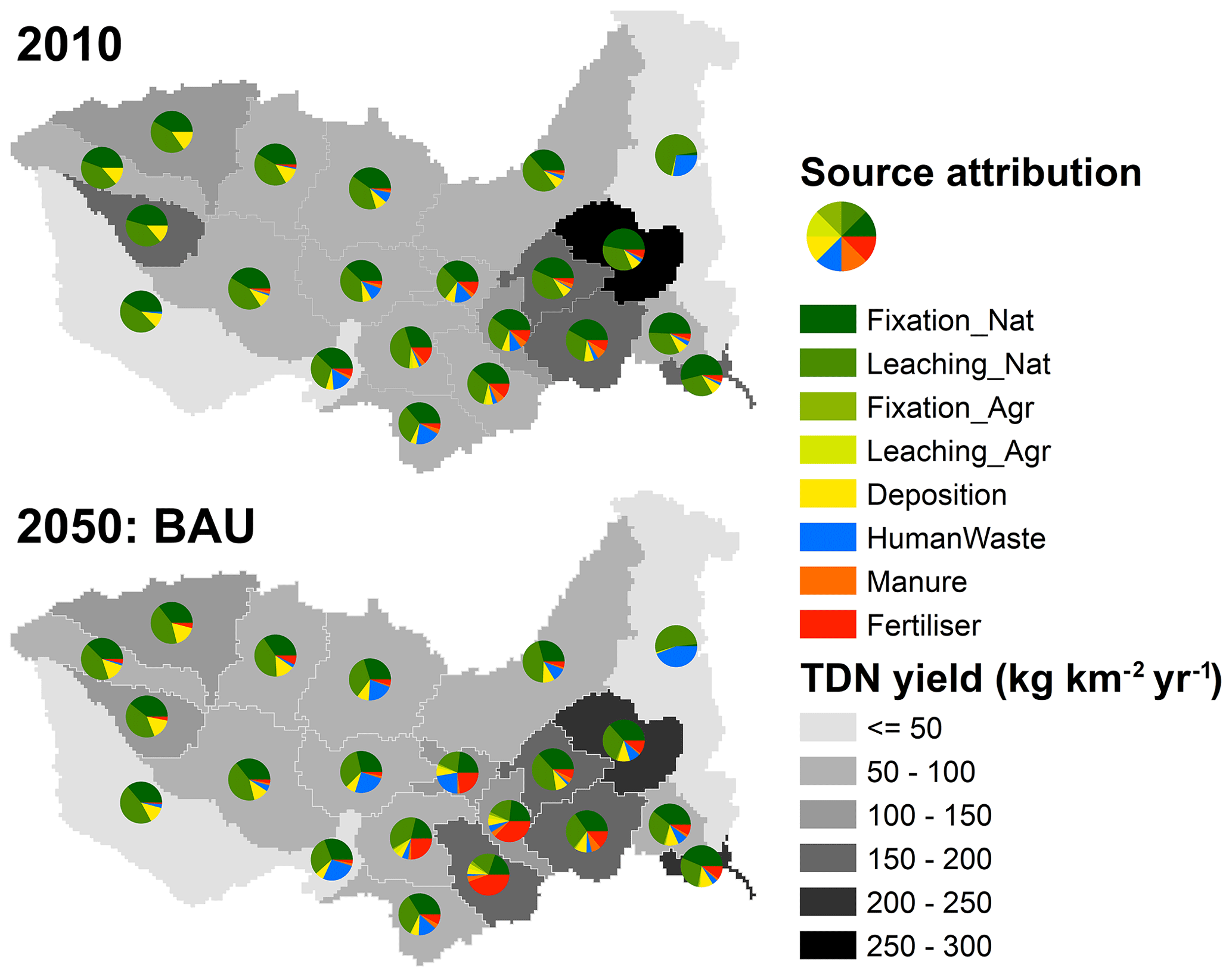
Figure 16Increase in river export of total dissolved nitrogen to sea between 2010 and 2050 (business-as-usual scenario).
Figure 17 is an example of ECHO simulation results. It shows the costs for water supply and management in order to satisfy sectoral water demands (irrigation, livestock, domestic, and industrial) and environmental constraints (i.e., minimum environmental flow requirements and groundwater sustainability constraints) in the Zambezi river basin over the 2010–2050 period.
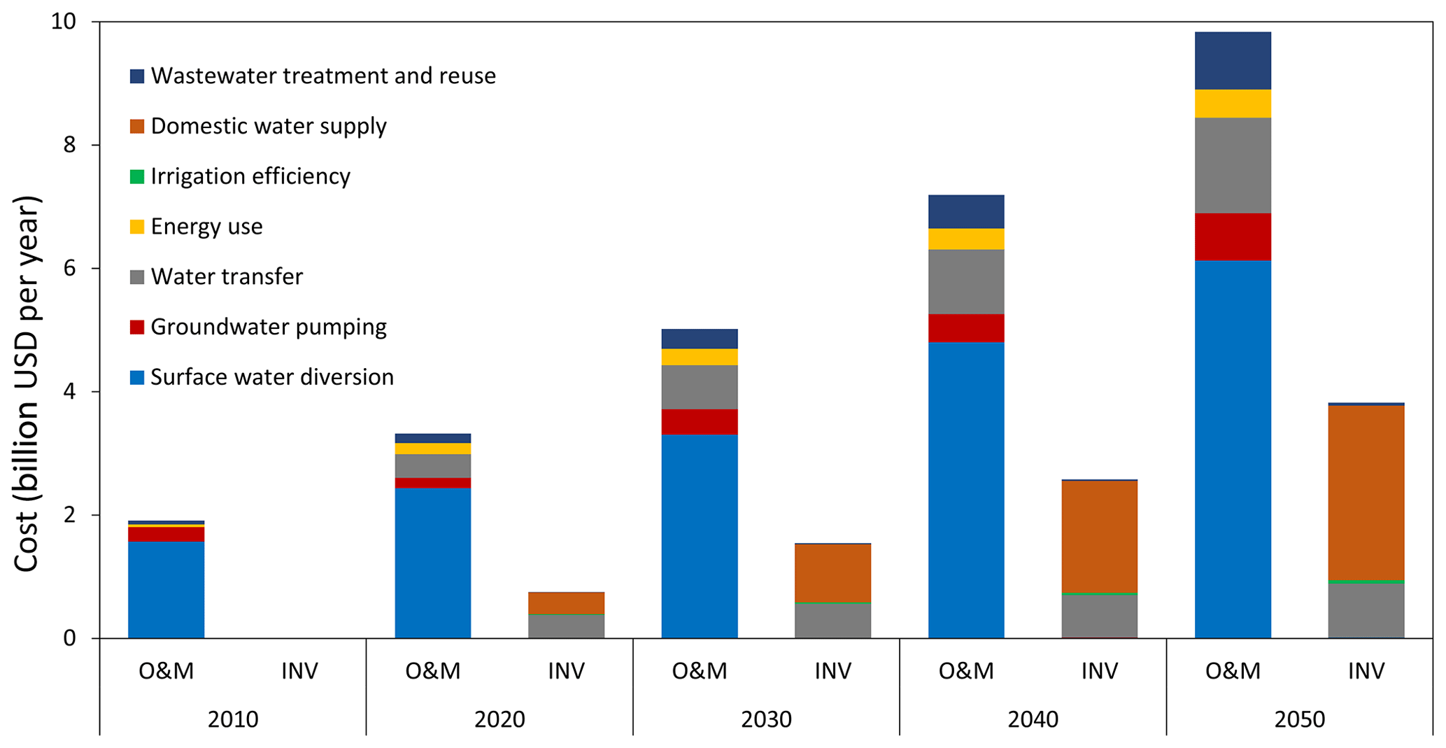
Figure 17Investment (INV) and operating (O&M) costs for water supply and management in the Zambezi basin between 2010 and 2050 (business-as-usual scenario).
We presented the new global hydrological model CWatM, which can be used globally and regionally at different resolutions with different datasets. The model is open source in the Python environment and has a flexible modular structure. It uses global, freely available data in the state-of-the art format of netCDF4 files to store and produce data in a compact way. It includes major hydrological processes but also takes human water use into account by calculating water demand, water consumption, and return flows. Reservoirs and lakes are included in the model scheme. CWatM is being developed to include a routing scheme related to reservoirs and canals to better simulate water availability in both agricultural and urban contexts.
It is shown that CWatM can be used in the framework of ISIMIP as a global model and also as part of a model integration of hydrological, hydro-economic, and water quality models for assessing and evaluating water management options. This study also presented the need for a hydrological model to be calibrated to be able to estimate a detailed regional balance of water demand and water availability.
An external limitation and a source of uncertainty is the quality of meteorological forcing driving the hydrological models. As shown in Müller Schmied et al. (2014), there are still discrepancies among the CMIP5 datasets and among the datasets and observations. The use of CMIP6 datasets (Eyring et al., 2016) is expected to reduce these uncertainties. Another external model limitation and source of uncertainty is the availability of gauging station data, which is generally globally decreasing, completely unavailable, or difficult to access for some parts of the world. Continuous, consistent, and long-term river discharge data as an integral parameter over the whole basin are essential for basin modeling, water resources management, and flood forecasting. Although the model represents the key hydrological processes, the groundwater model is relatively simple. But groundwater assessments (e.g., Bierkens et al., 2019) are becoming more and more important, as also is the importance of including lateral processes that increase the resolution of the model. Some other hydrological processes representation, e.g., evaporation from swamps, namely, the Sudd in the Nile basin and the Niger river swamps, need to be improved. The main direction of improvement should be better representation of human activities, e.g., management of reservoirs, including intra- and interbasin water transfer, and improving water demand requirements from agricultural sector by including irrigation schemes and plant phenology.
Future work will include (1) intensifying the development of a full dynamic coupling with a 2D groundwater model, (2) developing a global calibration scheme that also takes sparse observation of discharge into account, (3) a finer-resolution setting for 1 km working for the upper Bhima basin in India as part of the Food–Water–Energy for Urban Sustainable Environments project (https://fuse.stanford.edu, last access: 27 July 2020) supported by the Belmont Forum, (4) an interdisciplinary project aimed at better understanding the effect of certain nexus policy interventions and solution options linked to ECHO and beyond, and (5) improving software management by building up an automated testing, easier installation via the Python Package Index, and building containers and improving communication with the users.
CWatM is written in Python 3.7 and C as an open-source project under the term of the GNU General Public License version 3. License and download information are at https://cwatm.iiasa.ac.at/license.html (last access: 27 July 2020). The code can be used on different platforms (Unix, Linux, Windows, Mac) and is provided through a GitHub repository: https://github.com/cwatm/cwatm (CWatM github sourcecode, 2020). It comes with the code, an executable program for Windows, a test case (river Rhine basin), and a settings file, as well as some tools such as the calibration routine. The version of the model used to produce the results in this paper is stored as version 1.04 in the GitHub repository and at Zenodo with the associated DOI: https://doi.org/10.5281/zenodo.3361478 (Burek et al., 2019). A global dataset at 0.5∘ and a dataset for the river Rhine are stored at https://doi.org/10.5281/zenodo.3528098 (Burek and Satoh, 2019).
Climate forcing data can be found on the ISI-MIP server (Frieler et al., 2016) or any other climate forcing dataset stored as netcdf can be used. Online documentation including documentation on the source code can be found on https://cwatm.iiasa.ac.at (last access: 27 July 2020). Development and maintenance of the official version of CWatM is conducted by the IIASA Water Program. Contribution, ideas, and users are very welcome. Global data for 0.5∘ or 5′ can be requested and stored on an IIASA FTP server.
The supplement related to this article is available online at: https://doi.org/10.5194/gmd-13-3267-2020-supplement.
PB wrote the original draft, prepared the manuscript and is main developer of the software; YS contributed to the water demand software development; TK contributed to the methodology writing and the results part of linking to hydro-economic modeling and produced Fig. 17; TT contributed to the methodology writing and the results part of linking to water quality and produced Figs. 15 and 16. PG, MS and LG all contributed to software development of the evaporation, water demand and groundwater modules. FZ provided processed daily observation data for the calibration validation, and YW coordinated the funding acquisition and contributed to conceptualization, methodology writing and reviewing.
The author declares that there is no conflict of interest.
The authors acknowledge the Global Environment Facility (GEF) for funding the development of this research and the CWatM model development as a part of the Integrated Solutions for Water, Energy, and Land (ISWEL) project (GEF Contract Agreement: 6993) and the support of the United Nations Industrial Development Organization (UNIDO). The authors also acknowledge the continuous support of the Asian Development Bank (ADB), the Austrian Development Agency (ADA), and the Austrian Federal Ministry of Sustainability and Tourism to the Water Futures and Solutions (WFaS) initiative at Water Program of IIASA. This study and the model development were also conducted as part of the Belmont Forum Sustainable Urbanisation Global Initiative (SUGI)/Food–Water–Energy Nexus theme for which coordination was supported by the US National Science Foundation under grant ICER/EAR-1829999 to Stanford University. The Global Runoff Data Centre (GRDC, Koblenz, Germany) is thanked for providing the observed discharge data. We appreciate all the other open-source projects which we used to collect ideas and which, on the other side, we hope to cross-fertilize with our ideas. We are very grateful to all the freely available datasets. Any opinions, findings, and conclusions or recommendations expressed in this material do not necessarily reflect the views of the funding organizations. This study is also partly supported by financial support from the Austrian Research Promotion Agency (FFG) under the FUSE project funded by the Belmont Forum (grant agreement: 730254), the EUCP (European Climate Prediction System) project funded by the European Union under Horizon 2020 (grant agreement: 776613), and CO-MICC project which is part of ERA4CS, an ERA-NET initiated by JPI Climate with co-funding by the European Union and the Austrian Federal Ministry of Science, Research and Economy (BMWFW).
This study and the model development were also conducted as part of the Belmont Forum Sustainable Urbanisation Global Initiative (SUGI)/Food–Water–Energy Nexus theme for which coordination was supported by the US National Science Foundation under grant ICER/EAR-1829999 to Stanford University. This study is also partly supported by financial support from the Austrian Research Promotion Agency (FFG) under the FUSE project funded by the Belmont Forum (Grant Agreement: 730254), EUCP (European Climate Prediction System) project funded by the European Union under Horizon 2020 (Grant Agreement: 776613), and CO-MICC project which is part of ERA4CS, an ERA-NET initiated by JPI Climate with co-funding by the European Union and the Austrian Federal Ministry of Science, Research and Economy (BMWFW).
This paper was edited by Wolfgang Kurtz and reviewed by three anonymous referees.
Alcamo, J., Döll, P., Henrichs, T., Kaspar, F., Lehner, B., Rösch, T., and Siebert, S.: Development and testing of the WaterGAP 2 global model of water use and availability, Hydrolog. Sci. J., 48, 317–338, https://doi.org/10.1623/hysj.48.3.317.45290, 2003.
Alcamo, J., Flörke, M., and Märker, M.: Future long-term changes in global water resources driven by socio-economic and climatic changes, Hydrolog. Sci. J., 52, 247–275, https://doi.org/10.1623/hysj.52.2.247, 2007.
Allen, R. G., Pereira, L. S., Raes, D., and Smith, M.: Crop evapotranspiration-Guidelines for computing crop water requirements-FAO Irrigation and drainage paper 56, FAO, Rome, 300, D05109, 1998.
Anderson, E.: Snow Accumulation and Ablation Model – SNOW-17, Technical report, 2006.
Bakker, M., Post, V., Langevin, C. D., Hughes, J. D., White, J. T., Starn, J. J., and Fienen, M. N.: Scripting MODFLOW Model Development Using Python and FloPy, Groundwater, 54, 733–739, https://doi.org/10.1111/gwat.12413, 2016.
Balkovič, J., van der Velde, M., Skalský, R., Xiong, W., Folberth, C., Khabarov, N., Smirnov, A., Mueller, N. D., and Obersteiner, M.: Global wheat production potentials and management flexibility under the representative concentration pathways, Global Planet. Change, 122, 107–121, doi.org/10.1016/j.gloplacha.2014.08.010, 2014.
Beck, H. E., van Dijk, A. I. J. M., de Roo, A., Miralles, D. G., McVicar, T. R., Schellekens, J., and Bruijnzeel, L. A.: Global-scale regionalization of hydrologic model parameters, Water Resour. Res., 52, 3599–3622, https://doi.org/10.1002/2015WR018247, 2016.
Beck, H. E., van Dijk, A. I. J. M., Levizzani, V., Schellekens, J., Miralles, D. G., Martens, B., and de Roo, A.: MSWEP: 3-hourly 0.25∘ global gridded precipitation (1979–2015) by merging gauge, satellite, and reanalysis data, Hydrol. Earth Syst. Sci., 21, 589–615, https://doi.org/10.5194/hess-21-589-2017, 2017.
Bergstrom, S.: Principles and confidence in hydrological modelling, Nord. Hydrol., 22, 123–136, 1991.
Bergström, S. and Forsman, A.: Development of a conceptual deterministic rainfall-runoff model, Nord. Hydrol., 4, 147–170, 1973.
Bierkens, M. F. P.: Global hydrology 2015: State, trends, and directions, Water Resour. Res., 51, 4923–4947, https://doi.org/10.1002/2015WR017173, 2015.
Bierkens, M. F. P., Reinhard, S., de Bruijn, J. A., Veninga, W., and Wada, Y.: The Shadow Price of Irrigation Water in Major Groundwater-Depleting Countries, Water Resour. Res., 55, 4266–4287, https://doi.org/10.1029/2018WR023086, 2019.
Bollrich, G. and Preißler, G.: Technische Hydromechanik – Grundlagen, Beuth Verlag GmbH Berlin, Wien, Zürich, 449 pp., 1992.
Bondeau, A., Smith, P. C., Zaehle, S., Schaphoff, S., Lucht, W., Cramer, W., Gerten, D., Lotze-campen, H., Müller, C., Reichstein, M., and Smith, B.: Modelling the role of agriculture for the 20th century global terrestrial carbon balance, Glob. Change Biol., 13, 679–706, https://doi.org/10.1111/j.1365-2486.2006.01305.x, 2007.
Burek, P. and Satoh, Y.: CWATM v1.04 – 0.5 deg dataset (Version v1.04) [Data set], Zenodo, https://doi.org/10.5281/zenodo.3528098, 2019.
Burek, P., van der Knijff, J., and de Roo, A.: LISFLOOD Distributed Water Balance and Flood Simulation Model, European Commission, Joint Research Centre, Institute for Environment and Sustainability, Luxembourg, 2013.
Burek, P., Satoh, Y., Fischer, G., Kahil, M. T., Scherzer, A., Tramberend, S., Nava, L. F., Wada, Y., Eisner, S., Flörke, M., Hanasaki, N., Magnuszewski, P., Cosgrove, B., and Wiberg, D.: Water Futures and Solution – Fast Track Initiative (Final Report), IIASA, Laxenburg, Austria, IIASA Working Paper, 2016.
Burek, P., Smilovic, M., Satoh, Y., Kahil, T., Guillaumot, L., Tang, T., and Wada, Y.: Community Water Model (CwatM) (Version v1.04), Zenodo, https://doi.org/10.5281/zenodo.3361478, 2019.
Chow, V. T., Maidment, D. R., and Mays, L. W.: Applied hydrology, McGraw-Hill, New York, 1998.
Clark, M. P., Kavetski, D., and Fenicia, F.: Pursuing the method of multiple working hypotheses for hydrological modeling, Water Resour. Res., 47, https://doi.org/10.1029/2010WR009827, 2011.
Clark, M. P., Nijssen, B., Lundquist, J. D., Kavetski, D., Rupp, D. E., Woods, R. A., Freer, J. E., Gutmann, E. D., Wood, A. W., Brekke, L. D., Arnold, J. R., Gochis, D. J., and Rasmussen, R. M.: A unified approach for process-based hydrologic modeling: 1. Modeling concept, Water Resour. Res., 51, 2498–2514, https://doi.org/10.1002/2015WR017198, 2015.
CWatM github sourcecode: available at: https://github.com/cwatm/cwatm, last access: 27 July 2020.
Deb, K., Pratap, A., Agarwal, S., and Meyarivan, T.: A fast and elitist multiobjective genetic algorithm: NSGA-II, IEEE T. Evolut. Comput., 6, 182–197, https://doi.org/10.1109/4235.996017, 2002.
Decharme, B., Delire, C., Minvielle, M., Colin, J., Vergnes, J. P., Alias, A., Saint-Martin, D., Séférian, R., Sénési, S., and Voldoire, A.: Recent Changes in the ISBA-CTRIP Land Surface System for Use in the CNRM-CM6 Climate Model and in Global Off-Line Hydrological Applications, J. Adv. Model. Earth Sy., 11, 1207–1252, https://doi.org/10.1029/2018MS001545, 2019.
de Graaf, I. E. M., van Beek, L. P. H., Wada, Y., and Bierkens, M. F. P.: Dynamic attribution of global water demand to surface water and groundwater resources: Effects of abstractions and return flows on river discharges, Adv. Water Resour., 64, 21–33, https://doi.org/10.1016/j.advwatres.2013.12.002, 2014.
de Graaf, I. E. M., Sutanudjaja, E. H., van Beek, L. P. H., and Bierkens, M. F. P.: A high-resolution global-scale groundwater model, Hydrol. Earth Syst. Sci., 19, 823–837, https://doi.org/10.5194/hess-19-823-2015, 2015.
de Graaf, I. E. M., van Beek, R. L. P. H., Gleeson, T., Moosdorf, N., Schmitz, O., Sutanudjaja, E. H., and Bierkens, M. F. P.: A global-scale two-layer transient groundwater model: Development and application to groundwater depletion, Adv. Water Resour., 102, 53–67, https://doi.org/10.1016/j.advwatres.2017.01.011, 2017.
De Roo, A. P. J., Wesseling, C. G., and Van Deursen, W. P. A.: Physically based river basin modelling within a GIS: The LISFLOOD model, Hydrol. Process., 14, 1981–1992, 2000.
Döll, P. and Lehner, B.: Validation of a new global 30-min drainage direction map, J. Hydrol., 258, 214–231, https://doi.org/10.1016/S0022-1694(01)00565-0, 2002.
Döll, P. and Siebert, S.: Global modeling of irrigation water requirements, Water Resour. Res., 38, 81–811, 2002.
Döll, P., Fiedler, K., and Zhang, J.: Global-scale analysis of river flow alterations due to water withdrawals and reservoirs, Hydrol. Earth Syst. Sci., 13, 2413–2432, https://doi.org/10.5194/hess-13-2413-2009, 2009.
Döll, P., Fritsche, M., Eicker, A., and Müller Schmied, H.: Seasonal Water Storage Variations as Impacted by Water Abstractions: Comparing the Output of a Global Hydrological Model with GRACE and GPS Observations, Surv. Geophys., 35, 1311–1331, https://doi.org/10.1007/s10712-014-9282-2, 2014.
EAC: East African Community Vision 2050, Regional Vision for Socio-Economic Tranformation and Development, East African Vision (EAC), Arusha, Tanzania, 2016.
EEA: The European Environment – State and Outlook 2005, European Environment Agency, Copenhagen, 2005.
Elvidge, C. D., Tuttle, B. T., Sutton, P. S., Baugh, K. E., Howard, A. T., Milesi, C., Bhaduri, B. L., and Nemani, R.: Global distribution and density of constructed impervious surfaces, Sensors, 7, 1962–1979, https://doi.org/10.3390/s7091962, 2007.
Eyring, V., Bony, S., Meehl, G. A., Senior, C. A., Stevens, B., Stouffer, R. J., and Taylor, K. E.: Overview of the Coupled Model Intercomparison Project Phase 6 (CMIP6) experimental design and organization, Geosci. Model Dev., 9, 1937–1958, https://doi.org/10.5194/gmd-9-1937-2016, 2016.
Falkenmark, M.: Meeting water requirements of an expanding world population, Philos. T. Roy. Soc. B, 352, 929–936, https://doi.org/10.1098/rstb.1997.0072, 1997.
Falkenmark, M., Lundqvist, J., and Widstrand, C.: Macro-scale water scarcity requires micro-scale approaches, Nat. Resour. Forum, 13, 258–267, 1989.
FAO: Gridded livestock of the world, Food and Agriculture Organization of the United Nations, Rome, 131 pp., 2007.
FAO: FAOSTAT online database, available at: http://www.fao.org/faostat (last access: 27June 2020), 2012.
FAO, IIASA, ISRIC, ISSCAS, and JRC: Harmonized World Soil Database (version 1.2). FAO, Rome, Italy and IIASA, Laxenburg, Austria, 2012.
Fick, S. E. and Hijmans, R. J.: Worldclim 2: New 1-km spatial resolution climate surfaces for global land areas, Int. J. Climatol., 37, 4302–4315, https://doi.org/10.1002/joc.5086, 2017.
Flörke, M., Kynast, E., Bärlund, I., Eisner, S., Wimmer, F., and Alcamo, J.: Domestic and industrial water uses of the past 60 years as a mirror of socio-economic development: A global simulation study, Global Environ. Chang., 23, 144–156, 2013.
Fortin, F. A., De Rainville, F. M., Gardner, M. A., Parizeau, M., and Gagńe, C.: DEAP: Evolutionary algorithms made easy, J. Mach. Learn. Res., 13, 2171–2175, 2012.
Frenken, K. and Gillet, V.: Irrigation water requirement and water withdrawal by country, Rome, 2012.
Frieler, K., Lange, S., Piontek, F., Reyer, C. P. O., Schewe, J., Warszawski, L., Zhao, F., Chini, L., Denvil, S., Emanuel, K., Geiger, T., Halladay, K., Hurtt, G., Mengel, M., Murakami, D., Ostberg, S., Popp, A., Riva, R., Stevanovic, M., Suzuki, T., Volkholz, J., Burke, E., Ciais, P., Ebi, K., Eddy, T. D., Elliott, J., Galbraith, E., Gosling, S. N., Hattermann, F., Hickler, T., Hinkel, J., Hof, C., Huber, V., Jägermeyr, J., Krysanova, V., Marcé, R., Müller Schmied, H., Mouratiadou, I., Pierson, D., Tittensor, D. P., Vautard, R., van Vliet, M., Biber, M. F., Betts, R. A., Bodirsky, B. L., Deryng, D., Frolking, S., Jones, C. D., Lotze, H. K., Lotze-Campen, H., Sahajpal, R., Thonicke, K., Tian, H., and Yamagata, Y.: Assessing the impacts of 1.5 ∘C global warming – simulation protocol of the Inter-Sectoral Impact Model Intercomparison Project (ISIMIP2b), Geosci. Model Dev., 10, 4321–4345, https://doi.org/10.5194/gmd-10-4321-2017, 2017.
Gao, J.: Downscaling Global Spatial Population Projections from 1/8-degree to 1-km Grid Cells, National Center for Atmospheric Research, Boulder, CO, USA, 2017.
Gidden, M. J., Fujimori, S., van den Berg, M., Klein, D., Smith, S. J., van Vuuren, D. P., and Riahi, K.: A methodology and implementation of automated emissions harmonization for use in Integrated Assessment Models, Environ. Modell. Softw., 105, 187–200, https://doi.org/10.1016/j.envsoft.2018.04.002, 2018.
Gleason, C. J., Wada, Y., and Wang, J.: A Hybrid of Optical Remote Sensing and Hydrological Modeling Improves Water Balance Estimation, J. Adv. Model. Earth Sy., 10, 2–17, https://doi.org/10.1002/2017MS000986, 2018.
Gleeson, T., Smith, L., Moosdorf, N., Hartmann, J., Dürr, H. H., Manning, A. H., Van Beek, L. P. H., and Jellinek, A. M.: Mapping permeability over the surface of the Earth, Geophys. Res. Lett., 38, 3891–3898, https://doi.org/10.1029/2010GL045565, 2011.
Gleeson, T., Moosdorf, N., Hartmann, J., and Van Beek, L. P. H.: A glimpse beneath earth's surface: GLobal HYdrogeology MaPS (GLHYMPS) of permeability and porosity, Geophys. Res. Lett., 41, 3891–3898, https://doi.org/10.1002/2014GL059856, 2014.
Gleick, P. H., Cooley, H., Cohen, M. J., Morikawa, M., Morrison, J., and Palaniappan, M.: The Worlds Water 2008–2009, The Biennial Report on Freshwater Resources, DC, USA, 2009.
GRDC: Major River Basins of the World / Global Runoff Data Centre, GRDC, Koblenz, Germany, Federal Institute of Hydrology (BfG), 2007.
Greve, P., Gudmundsson, L., Orlowsky, B., and Seneviratne, S. I.: A two-parameter Budyko function to represent conditions under which evapotranspiration exceeds precipitation, Hydrol. Earth Syst. Sci., 20, 2195–2205, https://doi.org/10.5194/hess-20-2195-2016, 2016.
Gupta, H. V., Kling, H., Yilmaz, K. K., and Martinez, G. F.: Decomposition of the mean squared error and NSE performance criteria: Implications for improving hydrological modelling, J. Hydrol., 377, 80–91, https://doi.org/10.1016/j.jhydrol.2009.08.003, 2009.
Habets, F., Boone, A., Champeaux, J. L., Etchevers, P., Franchistéguy, L., Leblois, E., Ledoux, E., Le Moigne, P., Martin, E., Morel, S., Noilhan, J., Seguí, P. Q., Rousset-Regimbeau, F., and Viennot, P.: The SAFRAN-ISBA-MODCOU hydrometeorological model applied over France, J. Geophys. Res.-Atmos., 113, D06113, https://doi.org/10.1029/2007JD008548, 2008.
Haddeland, I., Clark, D. B., Franssen, W., Ludwig, F., Voß, F., Arnell, N. W., Bertrand, N., Best, M., Folwell, S., Gerten, D., Gomes, S., Gosling, S. N., Hagemann, S., Hanasaki, N., Harding, R., Heinke, J., Kabat, P., Koirala, S., Oki, T., Polcher, J., Stacke, T., Viterbo, P., Weedon, G. P., and Yeh, P.: Multimodel estimate of the global terrestrial water balance: Setup and first results, J. Hydrometeorol., 12, 869–884, https://doi.org/10.1175/2011JHM1324.1, 2011.
Hamon, W.: Computation of Direct Runoff Amounts from Storm Rainfall, IAHS Publ., 63, 52–62, 1963.
Hanasaki, N., Kanae, S., and Oki, T.: A reservoir operation scheme for global river routing models, J. Hydrol., 327, 22–41, https://doi.org/10.1016/j.jhydrol.2005.11.011, 2006.
Hanasaki, N., Kanae, S., Oki, T., Masuda, K., Motoya, K., Shirakawa, N., Shen, Y., and Tanaka, K.: An integrated model for the assessment of global water resources – Part 1: Model description and input meteorological forcing, Hydrol. Earth Syst. Sci., 12, 1007–1025, https://doi.org/10.5194/hess-12-1007-2008, 2008.
Hanasaki, N., Yoshikawa, S., Pokhrel, Y., and Kanae, S.: A global hydrological simulation to specify the sources of water used by humans, Hydrol. Earth Syst. Sci., 22, 789–817, https://doi.org/10.5194/hess-22-789-2018, 2018.
Hansen, M. C., Potapov, P. V., Moore, R., Hancher, M., Turubanova, S. A., Tyukavina, A., Thau, D., Stehman, S. V., Goetz, S. J., Loveland, T. R., Kommareddy, A., Egorov, A., Chini, L., Justice, C. O., and Townshend, J. R. G.: High-resolution global maps of 21st-century forest cover change, Science, 342, 850–853, https://doi.org/10.1126/science.1244693, 2013.
Harbaugh, A. W.: MODFLOW-2005, the U.S. Geological survey modular ground-water model – The ground-water flow process, 2005.
Hargreaves, G. H. and Samani, Z. A.: Reference crop evapotranspiration from temperature, Appl. Eng. Agric., 1, 96–99, 1958.
Hartmann, A., Gleeson, T., Rosolem, R., Pianosi, F., Wada, Y., and Wagener, T.: A large-scale simulation model to assess karstic groundwater recharge over Europe and the Mediterranean, Geosci. Model Dev., 8, 1729–1746, https://doi.org/10.5194/gmd-8-1729-2015, 2015.
Havlík, P., Valin, H., Mosnier, A., Obersteiner, M., Baker, J. S., Herrero, M., Rufino, M. C., and Schmid, E.: Crop productivity and the global livestock sector: Implications for land use change and greenhouse gas emissions, Am. J. Agr. Econ., 95, 442–448, https://doi.org/10.1093/ajae/aas085, 2013.
He, X., Feng, K., Li, X., Craft, A. B., Wada, Y., Burek, P., Wood, E. F., and Sheffield, J.: Solar and wind energy enhances drought resilience and groundwater sustainability, Nat. Commun., 10, 4893, https://doi.org/10.1038/s41467-019-12810-5, 2019.
Hrachowitz, M., Savenije, H. H. G., Blöschl, G., McDonnell, J. J., Sivapalan, M., Pomeroy, J. W., Arheimer, B., Blume, T., Clark, M. P., Ehret, U., Fenicia, F., Freer, J. E., Gelfan, A., Gupta, H. V., Hughes, D. A., Hut, R. W., Montanari, A., Pande, S., Tetzlaff, D., Troch, P. A., Uhlenbrook, S., Wagener, T., Winsemius, H. C., Woods, R. A., Zehe, E., and Cudennec, C.: A decade of Predictions in Ungauged Basins (PUB) – a review, Hydrolog. Sci. J., 58, 1198–1255, https://doi.org/10.1080/02626667.2013.803183, 2013.
Huscroft, J., Gleeson, T., Hartmann, J., and Börker, J.: Compiling and Mapping Global Permeability of the Unconsolidated and Consolidated Earth: GLobal HYdrogeology MaPS 2.0 (GLHYMPS 2.0), Geophys. Res. Lett., 45, 1897–1904, https://doi.org/10.1002/2017GL075860, 2018.
Jarvis, A., Reuter, H. I., Nelson, A., and Guevara, E.: Hole-filled SRTM for the globe Version 4, available from the CGIAR-CSI SRTM 90m Database http://srtm.csi.cgiar.org (last access: 27 June 2020), 2008.
Jiang, L. and O'Neill, B. C.: Global urbanization projections for the Shared Socioeconomic Pathways, Global Environ. Chang., 42, 193–199, https://doi.org/10.1016/j.gloenvcha.2015.03.008, 2017.
Jiménez, R. C., Kuzak, M., Alhamdoosh, M., Barker, M., Batut, B., Borg, M., Capella-Gutierrez, S., Chue Hong, N., Cook, M., Corpas, M., Flannery, M., Garcia, L., Gelpí, J. L., Gladman, S., Goble, C., González Ferreiro, M., Gonzalez-Beltran, A., Griffin, P. C., Grüning, B., Hagberg, J., Holub, P., Hooft, R., Ison, J., Katz, D. S., Leskošek, B., López Gómez, F., Oliveira, L. J., Mellor, D., Mosbergen, R., Mulder, N., Perez-Riverol, Y., Pergl, R., Pichler, H., Pope, B., Sanz, F., Schneider, M. V., Stodden, V., Suchecki, R., Svobodová Vařeková, R., Talvik, H. A., Todorov, I., Treloar, A., Tyagi, S., van Gompel, M., Vaughan, D., Via, A., Wang, X., Watson-Haigh, N. S., and Crouch, S.: Four simple recommendations to encourage best practices in research software, F1000Research, 6, https://doi.org/10.12688/f1000research.11407.1, 2017.
Jones, B. and O'Neill, B. C.: Spatially explicit global population scenarios consistent with the Shared Socioeconomic Pathways, Environ. Res. Lett., 11, 084003, https://doi.org/10.1088/1748-9326/11/8/084003, 2016.
Kahil, M. T., Parkinson, S., Satoh, Y., Greve, P., Burek, P., Veldkamp, T. I. E., Burtscher, R., Byers, E., Djilali, N., Fischer, G., Krey, V., Langan, S., Riahi, K., Tramberend, S., and Wada, Y.: A Continental-Scale Hydroeconomic Model for Integrating Water-Energy-Land Nexus Solutions, Water Resour. Res., 54, 7511–7533, https://doi.org/10.1029/2017WR022478, 2018.
Kahil, T., Albiac, J., Fischer, G., Strokal, M., Tramberend, S., Greve, P., Tang, T., Burek, P., Burtscher, R., and Wada, Y.: A nexus modeling framework for assessing water scarcity solutions, Curr. Opin. Env. Sust., 40, 72–80, https://doi.org/10.1016/j.cosust.2019.09.009, 2019.
Karssenberg, D., Schmitz, O., Salamon, P., de Jong, K., and Bierkens, M. F. P.: A software framework for construction of process-based stochastic spatio-temporal models and data assimilation, Environ. Modell. Softw., 25, 489–502, https://doi.org/10.1016/j.envsoft.2009.10.004, 2010.
Kauffeldt, A., Wetterhall, F., Pappenberger, F., Salamon, P., and Thielen, J.: Technical review of large-scale hydrological models for implementation in operational flood forecasting schemes on continental level, Environ. Modell. Softw., 75, 68–76, https://doi.org/10.1016/j.envsoft.2015.09.009, 2016.
Kim, H., Watanabe, S., Chang, E.-C., Yoshimura, K., Hirabayashi, Y., Famiglietti, J., and Oki, T.: Century long observation constrained global dynamic downscaling and hydrologic implication, American Geophysical Union, Fall Meeting 2012, 2012.
Klein Goldewijk, K., Beusen, A., Doelman, J., and Stehfest, E.: Anthropogenic land use estimates for the Holocene – HYDE 3.2, Earth Syst. Sci. Data, 9, 927–953, https://doi.org/10.5194/essd-9-927-2017, 2017.
Kling, H., Fuchs, M., and Paulin, M.: Runoff conditions in the upper Danube basin under an ensemble of climate change scenarios, J. Hydrol., 424–425, 264–277, https://doi.org/10.1016/j.jhydrol.2012.01.011, 2012.
Koirala, S., Yamada, H., Yeh, P., Oki, T., Hirabayashi, Y., and Kanae, S.: Global simulation of groundwater recharge, water ta-ble depth, and low flow using a land surface model with ground-water representation, Journal of Japan Society of Civil Engineers, 68, 211–216, https://doi.org/10.2208/jscejhe.68.I_211, 2012.
Kumar, R., Samaniego, L., and Attinger, S.: Implications of distributed hydrologic model parameterization on water fluxes at multiple scales and locations, Water Resour. Res., 49, 360–379, https://doi.org/10.1029/2012WR012195, 2013.
Kummu, M., Taka, M., and Guillaume, J. H. A.: Gridded global datasets for Gross Domestic Product and Human Development Index over 1990–2015, Scientific Data, 5, https://doi.org/10.1038/sdata.2018.4, 2018.
Lange, S.: Bias correction of surface downwelling longwave and shortwave radiation for the EWEMBI dataset, Earth Syst. Dynam., 9, 627–645, https://doi.org/10.5194/esd-9-627-2018, 2018.
Lehner, B., Liermann, C. R., Revenga, C., Vörösmarty, C., Fekete, B., Crouzet, P., Döll, P., Endejan, M., Frenken, K., Magome, J., Nilsson, C., Robertson, J. C., Rödel, R., Sindorf, N., and Wisser, D.: High-resolution mapping of the world's reservoirs and dams for sustainable river-flow management, Front. Ecol. Environ., 9, 494–502, https://doi.org/10.1890/100125, 2011.
Lindström, G.: A simple automatic calibration routine for the HBV model, Nord. Hydrol., 28, 153–168, 1997.
Lindström, G., Johansson, B., Persson, M., Gardelin, M., and Bergström, S.: Development and test of the distributed HBV-96 hydrological model, J. Hydrol., 201, 272–288, https://doi.org/10.1016/S0022-1694(97)00041-3, 1997.
Maniak, U.: Hydrologie und Wasserwirtschaft, Springer-Verlag Berlin Heidelberg, 651 pp., 1997.
McDonald, M. and Harbaugh, A.: A Modular Three-Dimensional Finite-Difference Ground-Water Flow Model: Techniques of Water Resources Investigations, Book 6, U.S. Geol. Sur, Denver, Colorado, USA, 1988.
Messager, M. L., Lehner, B., Grill, G., Nedeva, I., and Schmitt, O.: Estimating the volume and age of water stored in global lakes using a geo-statistical approach, Nat. Commun., 7, 13603, https://doi.org/10.1038/ncomms13603, 2016.
Mohan, C., Western, A. W., Wei, Y., and Saft, M.: Predicting groundwater recharge for varying land cover and climate conditions – a global meta-study, Hydrol. Earth Syst. Sci., 22, 2689–2703, https://doi.org/10.5194/hess-22-2689-2018, 2018.
Molnau, M. and Bissell, V. C.: A continuous frozen ground index for flood forecasting, Proceedings 51st Annual Meeting Western Snow Conference, 109–119, 1983.
Moreno, A. and Hasenauer, H.: Spatial downscaling of European climate data, Int. J. Climatol., 36, 1444–1458, https://doi.org/10.1002/joc.4436, 2016.
Mosier, T. M., Hill, D. F., and Sharp, K. V.: Update to the Global Climate Data package: analysis of empirical bias correction methods in the context of producing very high resolution climate projections, Int. J. Climatol., 38, 825–840, https://doi.org/10.1002/joc.5213, 2018.
Mualem, Y.: A New Model for Predicting the Hydraulic Conductivity of Unsaturated Porous Medial, Water Resour. Res., 12, 513–522, 1976.
Muller, P. J., Lewis, P., Fischer, J., North, P., and Framer, U.: The ESA GlobAlbedo Project for mapping the Earth's land surface albedo for 15 Years from European Sensors, paper presented at: IEEE Geoscience and Remote Sensing Symposium (IGARSS) 2012, Munich, Germany, 22–27 July 2012.
Müller Schmied, H., Eisner, S., Franz, D., Wattenbach, M., Portmann, F. T., Flörke, M., and Döll, P.: Sensitivity of simulated global-scale freshwater fluxes and storages to input data, hydrological model structure, human water use and calibration, Hydrol. Earth Syst. Sci., 18, 3511–3538, https://doi.org/10.5194/hess-18-3511-2014, 2014.
Pokhrel, Y.: Global Terrestrial Water Storage and Drought Severity under Climate Change, Nat. Clim. Change, in review, 2020.
Pokhrel, Y., Hanasaki, N., Koirala, S., Cho, J., Yeh, P. J. F., Kim, H., Kanae, S., and Oki, T.: Incorporating anthropogenic water regulation modules into a land surface model, J. Hydrometeorol., 13, 255–269, https://doi.org/10.1175/JHM-D-11-013.1, 2012.
Pokhrel, Y. N., Koirala, S., Yeh, P. J. F., Hanasaki, N., Longuevergne, L., Kanae, S., and Oki, T.: Incorporation of groundwater pumping in a global Land Surface Model with the representation of human impacts, Water Resour. Res., 51, 78–96, https://doi.org/10.1002/2014WR015602, 2015.
Pokhrel, Y. N., Hanasaki, N., Wada, Y., and Hyungjun, K.: Recent progresses in incorporating human land–water management into global land surface models toward their integration into Earth system models, WIREs Water, 3, 548–574, https://doi.org/10.1002/wat2.1150, 2016.
Portmann, F. T., Siebert, S., and Döll, P.: MIRCA2000–Global monthly irrigated and rainfed crop areas around the year 2000: A new high-resolution data set for agricultural and hydrological modeling, Global Biogeochem. Cy., 24, GB1011, https://doi.org/10.1029/2008GB003435, 2010.
Raskin, P., Gleick, P. H., Kirshen, P., Pontius, R. G., and Strzepek, K.: Comprehensive assessment of the freshwater resources of the world, Stockholm Environment Institute, Stockholm, Sweden, 1997.
Reinecke, R., Foglia, L., Mehl, S., Trautmann, T., Cáceres, D., and Döll, P.: Challenges in developing a global gradient-based groundwater model (G3M v1.0) for the integration into a global hydrological model, Geosci. Model Dev., 12, 2401–2418, https://doi.org/10.5194/gmd-12-2401-2019, 2019.
Revilla-Romero, B., Beck, H. E., Burek, P., Salamon, P., de Roo, A., and Thielen, J.: Filling the gaps: Calibrating a rainfall-runoff model using satellite-derived surface water extent, Remote Sens. Environ., 171, 118–131, https://doi.org/10.1016/j.rse.2015.10.022, 2015.
Riahi, K., van Vuuren, D. P., Kriegler, E., Edmonds, J., O'Neill, B. C., Fujimori, S., Bauer, N., Calvin, K., Dellink, R., Fricko, O., Lutz, W., Popp, A., Cuaresma, J. C., Kc, S., Leimbach, M., Jiang, L., Kram, T., Rao, S., Emmerling, J., Ebi, K., Hasegawa, T., Havlik, P., Humpenöder, F., Da Silva, L. A., Smith, S., Stehfest, E., Bosetti, V., Eom, J., Gernaat, D., Masui, T., Rogelj, J., Strefler, J., Drouet, L., Krey, V., Luderer, G., Harmsen, M., Takahashi, K., Baumstark, L., Doelman, J. C., Kainuma, M., Klimont, Z., Marangoni, G., Lotze-Campen, H., Obersteiner, M., Tabeau, A., and Tavoni, M.: The Shared Socioeconomic Pathways and their energy, land use, and greenhouse gas emissions implications: An overview, Global Environ. Chang., 42, 153–168, https://doi.org/10.1016/j.gloenvcha.2016.05.009, 2017.
Rost, S., Gerten, D., Bondeau, A., Lucht, W., Rohwer, J., and Schaphoff, S.: Agricultural green and blue water consumption and its influence on the global water system, Water Resour. Res., 44, W09405, https://doi.org/10.1029/2007WR006331, 2008.
Samaniego, L., Kumar, R., and Attinger, S.: Multiscale parameter regionalization of a grid-based hydrologic model at the mesoscale, Water Resour. Res., 46, W05523, https://doi.org/10.1029/2008WR007327, 2010.
Samaniego, L., Kumar, R., and Jackisch, C.: Predictions in a data-sparse region using a regionalized grid-based hydrologic model driven by remotely sensed data, Hydrol. Res., 42, 338–355, https://doi.org/10.2166/nh.2011.156, 2011.
Samaniego, L., Kumar, R., Thober, S., Rakovec, O., Zink, M., Wanders, N., Eisner, S., Müller Schmied, H., Sutanudjaja, E. H., Warrach-Sagi, K., and Attinger, S.: Toward seamless hydrologic predictions across spatial scales, Hydrol. Earth Syst. Sci., 21, 4323–4346, https://doi.org/10.5194/hess-21-4323-2017, 2017.
Scanlon, B. R., Zhang, Z., Save, H., Sun, A. Y., Schmied, H. M., Van Beek, L. P. H., Wiese, D. N., Wada, Y., Long, D., Reedy, R. C., Longuevergne, L., Döll, P., and Bierkens, M. F. P.: Global models underestimate large decadal declining and rising water storage trends relative to GRACE satellite data, P. Natl. Acad. Sci. USA, 115, E1080–E1089, https://doi.org/10.1073/pnas.1704665115, 2018.
Seidl, R. and Barthel, R.: Linking scientific disciplines: Hydrology and social sciences, J. Hydrol., 550, 441–452, https://doi.org/10.1016/j.jhydrol.2017.05.008, 2017.
Sheffield, J., Goteti, G., and Wood, E. F.: Development of a 50-year high-resolution global dataset of meteorological forcings for land surface modeling, J. Climate, 19, 3088–3111, https://doi.org/10.1175/JCLI3790.1, 2006.
Shen, Y., Oki, T., Utsumi, N., Kanae, S., and Hanasaki, N.: Projection of future world water resources under SRES scenarios: Water withdrawal, Hydrolog. Sci. J., 53, 11–33, https://doi.org/10.1623/hysj.53.1.11, 2008.
Shiklomanov, I. A.: Assessment of Water Resources and Water Availability in the World, Comprehensive Assessment of the Freshwater Re-sources of the World, 1997.
Shiklomanov, I. A.: Appraisal and Assessment of world water resources, Water Int., 25, 11–32, https://doi.org/10.1080/02508060008686794, 2000.
Siderius, C., Biemans, H., Kashaigili, J. J., and Conway, D.: Going local: Evaluating and regionalizing a global hydrological model's simulation of river flows in a medium-sized East African basin, J. Hydrol., 19, 349–364, https://doi.org/10.1016/j.ejrh.2018.10.007, 2018.
Siebert, S., Döll, P., Hoogeveen, J., Faures, J.-M., Frenken, K., and Feick, S.: Development and validation of the global map of irrigation areas, Hydrol. Earth Syst. Sci., 9, 535–547, https://doi.org/10.5194/hess-9-535-2005, 2005.
Siebert, S., Burke, J., Faures, J. M., Frenken, K., Hoogeveen, J., Döll, P., and Portmann, F. T.: Groundwater use for irrigation – a global inventory, Hydrol. Earth Syst. Sci., 14, 1863–1880, https://doi.org/10.5194/hess-14-1863-2010, 2010.
Sivapalan, M., Savenije, H. H. G., and Blöschl, G.: Socio-hydrology: A new science of people and water, Hydrol. Process., 26, 1270–1276, https://doi.org/10.1002/hyp.8426, 2012.
Speers, D. D. and Versteeg, J. D.: unoff forecasting for reservoir operations – the past and the future, Proceedings 52nd Western Snow Conference, 149–156, 1979.
Steinfeld, H., Gerber, P., Wassenaar, T., Castel, V., Rosales, M., and de Haan, C.: Livestock's long shadow: Environmental issues and options, Renewable Resources Journal, 24, 15–17, 2006.
Strokal, M., Kroeze, C., Wang, M., Bai, Z., and Ma, L.: The MARINA model (Model to Assess River Inputs of Nutrients to seAs): Model description and results for China, Sci. Total Environ., 562, 869–888, https://doi.org/10.1016/j.scitotenv.2016.04.071, 2016.
Sullivan, P., Krey, V., and Riahi, K.: Impacts of considering electric sector variability and reliability in the MESSAGE model, Energy Strateg. Rev., 1, 157–163, https://doi.org/10.1016/j.esr.2013.01.001, 2013.
Supit, I. and van der Goot, E.: Updated System Description of the WOFOST Crop Growth Simulation Model as Implemented in the Crop Growth Monitoring System Applied by the European Commission, Treemail, Heelsum, The Netherlands, 2003.
Supit, I., Hooijer, A. A., and van Diepen, C. A.: System Description of the WOFOST 6.0 Crop Simulation Model Implemented in CGMS, Office for Official Publications of the European Communities, Luxembourg, 1994.
Sutanudjaja, E. H., Van Beek, L. P. H., De Jong, S. M., Van Geer, F. C., and Bierkens, M. F. P.: Calibrating a large-extent high-resolution coupled groundwater-land surface model using soil moisture and discharge data, Water Resour. Res., 50, 687–705, https://doi.org/10.1002/2013WR013807, 2014.
Sutanudjaja, E. H., van Beek, R., Wanders, N., Wada, Y., Bosmans, J. H. C., Drost, N., van der Ent, R. J., de Graaf, I. E. M., Hoch, J. M., de Jong, K., Karssenberg, D., López López, P., Peßenteiner, S., Schmitz, O., Straatsma, M. W., Vannametee, E., Wisser, D., and Bierkens, M. F. P.: PCR-GLOBWB 2: a 5 arcmin global hydrological and water resources model, Geosci. Model Dev., 11, 2429–2453, https://doi.org/10.5194/gmd-11-2429-2018, 2018.
Tang, T., Strokal, M., Burek, P., Kroeze, C., van Vliet, M., and Wada, Y.: Sources and export of nutrients in the Zambezi River basin: status and future trend. In: International Conference Water Science for Impact, 16–18 October 2018, Wageningen, Netherlands, 2019.
Tapley, B. D., Bettadpur, S., Watkins, M., and Reigber, C.: The gravity recovery and climate experiment: Mission overview and early results, Geophys. Res. Lett., 31, L09607, https://doi.org/10.1029/2004GL019920, 2004.
Todini, E.: The ARNO rainfall – runoff model, J. Hydrol., 175, 339–382, 1996.
Tramberend, S., Burtscher, R., Burek, P., Kahil, T., Fischer, G., Mochizuki, J., Wada, Y., Kimwaga, R., Nyenje, P., Ondiek, R., Prossie, N., Hyandye, C., Sibomana, C., and Langan, S.: East Africa Future Water Scenarios to 2050, IIASA, Laxenburg, Austria, 2019.
Tramberend, S., Burtscher, R., Burek, P., Kahil, T., Fischer, G., Mochizuki, J., Kimwaga, R., Nyenje, P., Ondiek, R., Nakawuka, P., Hyandye, C., Sibomana, C., Luoga, H. P., Matano, A. S., Langan, S., and Wada, Y.: East African Community Water Vision. Regional Scenarios for Human – Natural Water System Transformations, ONE-EARTH-D-20-00017, https://doi.org/10.2139/ssrn.3526896, in review, 2020.
Udias, A., Gentile, A., Burek, P., De Roo, A., Bouraoui, F., Vandecasteele, I., Lavalle, C., and Bidoglio, G.: Multi-criteria framework to assess large scalewater resources policy measures, Water, 8, 370, https://doi.org/10.3390/w8090370, 2016.
UN-Water: Water Security & the Global Water Agenda,UNU-INWEH , Hamilton, Canada, ISBN 9789280860382, 2013.
USGS: Geological Survey Center for Earth Resources Observation and Science, Hydro1k, Land Processes Distributed Active Archive Center (LP DAAC), 2002.
Van Beek, L., Wada, Y., and Bierkens, M. F.: Global monthly water stress: 1. Water balance and water availability, Water Resour. Res., 47, W07517, https://doi.org/10.1029/2010WR009791, 2011.
Van Genuchten, M. T.: A closed-form equation for predicting the hydraulic conductivity of unsaturated soils, Science Society of America Journal, 44, 892–898, 1980.
van Vuuren, D. P., Edmonds, J., Kainuma, M., Riahi, K., Thomson, A., Hibbard, K., Hurtt, G. C., Kram, T., Krey, V., Lamarque, J. F., Masui, T., Meinshausen, M., Nakicenovic, N., Smith, S. J., and Rose, S. K.: The representative concentration pathways: An overview, Climatic Change, 109, 5–31, https://doi.org/10.1007/s10584-011-0148-z, 2011.
van Vuuren, D. P., Kriegler, E., O'Neill, B. C., Ebi, K. L., Riahi, K., Carter, T. R., Edmonds, J., Hallegatte, S., Kram, T., Mathur, R., and Winkler, H.: A new scenario framework for Climate Change Research: Scenario matrix architecture, Climatic Change, 122, 373–386, https://doi.org/10.1007/s10584-013-0906-1, 2014.
Vinca, A., Parkinson, S., Byers, E., Burek, P., Khan, Z., Krey, V., Diuana, F. A., Wang, Y., Ilyas, A., Köberle, A. C., Staffell, I., Pfenninger, S., Muhammad, A., Rowe, A., Schaeffer, R., Rao, N. D., Wada, Y., Djilali, N., and Riahi, K.: The NExus Solutions Tool (NEST) v1.0: an open platform for optimizing multi-scale energy–water–land system transformations, Geosci. Model Dev., 13, 1095–1121, https://doi.org/10.5194/gmd-13-1095-2020, 2020.
Viviroli, D., Zappa, M., Gurtz, J., and Weingartner, R.: An introduction to the hydrological modelling system PREVAH and its pre- and post-processing-tools, Environ. Modell. Softw., 24, 1209–1222, https://doi.org/10.1016/j.envsoft.2009.04.001, 2009.
Wada, Y.: Modeling Groundwater Depletion at Regional and Global Scales: Present State and Future Prospects, Surv. Geophys., 37, 419–451, https://doi.org/10.1007/s10712-015-9347-x, 2016.
Wada, Y., van Beek, L. P. H., and Bierkens, M. F. P.: Modelling global water stress of the recent past: on the relative importance of trends in water demand and climate variability, Hydrol. Earth Syst. Sci., 15, 3785–3808, https://doi.org/10.5194/hess-15-3785-2011, 2011.
Wada, Y., Wisser, D., and Bierkens, M. F. P.: Global modeling of withdrawal, allocation and consumptive use of surface water and groundwater resources, Earth Syst. Dynam., 5, 15–40, https://doi.org/10.5194/esd-5-15-2014, 2014.
Wada, Y., Flörke, M., Hanasaki, N., Eisner, S., Fischer, G., Tramberend, S., Satoh, Y., van Vliet, M. T. H., Yillia, P., Ringler, C., Burek, P., and Wiberg, D.: Modeling global water use for the 21st century: the Water Futures and Solutions (WFaS) initiative and its approaches, Geosci. Model Dev., 9, 175–222, https://doi.org/10.5194/gmd-9-175-2016, 2016.
Wada, Y., Bierkens, M. F. P., de Roo, A., Dirmeyer, P. A., Famiglietti, J. S., Hanasaki, N., Konar, M., Liu, J., Müller Schmied, H., Oki, T., Pokhrel, Y., Sivapalan, M., Troy, T. J., van Dijk, A. I. J. M., van Emmerik, T., Van Huijgevoort, M. H. J., Van Lanen, H. A. J., Vörösmarty, C. J., Wanders, N., and Wheater, H.: Human–water interface in hydrological modelling: current status and future directions, Hydrol. Earth Syst. Sci., 21, 4169–4193, https://doi.org/10.5194/hess-21-4169-2017, 2017.
Wang, M., Strokal, M., Burek, P., Kroeze, C., Ma, L., and Janssen, A. B. G.: Excess nutrient loads to Lake Taihu: Opportunities for nutrient reduction, Sci. Total Environ., 664, 865–873, https://doi.org/10.1016/j.scitotenv.2019.02.051, 2019a.
Wang, M., Tang, T., Burek, P., Havlík, P., Krisztin, T., Kroeze, C., Leclère, D., Strokal, M., Wada, Y., Wang, Y., and Langan, S.: Increasing nitrogen export to sea: A scenario analysis for the Indus River, Sci. Total Environ., 694, 133629, https://doi.org/10.1016/j.scitotenv.2019.133629, 2019b.
Warszawski, L., Frieler, K., Huber, V., Piontek, F., Serdeczny, O., and Schewe, J.: The inter-sectoral impact model intercomparison project (ISI–MIP): project framework, P. Natl. Acad. Sci. USA, 111, 3228–3232, 2014.
Weedon, G. P., Balsamo, G., Bellouin, N., Gomes, S., Best, M. J., and Viterbo, P.: The WFDEI meteorological forcing data set: WATCH Forcing data methodology applied to ERA-Interim reanalysis data, Water Resour. Res., 50, 7505–7514, https://doi.org/10.1002/2014WR015638, 2014.
Wilson, G., Aruliah, D. A., Brown, C. T., Chue Hong, N. P., Davis, M., Guy, R. T., Haddock, S. H. D., Huff, K. D., Mitchell, I. M., Plumbley, M. D., Waugh, B., White, E. P., and Wilson, P.: Best Practices for Scientific Computing, PLoS Biology, 12, e1001745, https://doi.org/10.1371/journal.pbio.1001745, 2014.
Wisser, D., Fekete, B. M., Vörösmarty, C. J., and Schumann, A. H.: Reconstructing 20th century global hydrography: a contribution to the Global Terrestrial Network- Hydrology (GTN-H), Hydrol. Earth Syst. Sci., 14, 1–24, https://doi.org/10.5194/hess-14-1-2010, 2010.
WMO: ntercomparison of models of snowmelt runoff, WMO- No. 646, Operational hydrology report (OHR) – No. 23, Geneva, Switzerland, 1986.
Wu, H., Kimball, J. S., Mantua, N., and Stanford, J.: Automated upscaling of river networks for macroscale hydrological modeling, Water Resour. Res., 47, W03517, https://doi.org/10.1029/2009WR008871, 2011.
Xu, L., Lettenmaier, D. P., Wood, E. F., and Burges, S. J.: A simple hydrologically based model of land surface water and energy fluxes for general circulation models, J. Geophys. Res., 99, 14+415–414+428, 1994.
Yates, D., Sieber, J., Purkey, D., and Huber-Lee, A.: WEAP21 – A demand-, priority-, and preference-driven water planning model. Part 1: Model characteristics, Water Int., 30, 487–500, https://doi.org/10.1080/02508060508691893, 2005.
Zhang, L., Dobslaw, H., Stacke, T., Güntner, A., Dill, R., and Thomas, M.: Validation of terrestrial water storage variations as simulated by different global numerical models with GRACE satellite observations, Hydrol. Earth Syst. Sci., 21, 821–837, https://doi.org/10.5194/hess-21-821-2017, 2017.
Zhang, Y. and Schaap, M. G.: Weighted recalibration of the Rosetta pedotransfer model with improved estimates of hydraulic parameter distributions and summary statistics (Rosetta3), J. Hydrol., 547, 39–53, https://doi.org/10.1016/j.jhydrol.2017.01.004, 2017.
Zhao, F., Veldkamp, T. I. E., Frieler, K., Schewe, J., Ostberg, S., Willner, S., Schauberger, B., Gosling, S. N., Schmied, H. M., Portmann, F. T., Leng, G., Huang, M., Liu, X., Tang, Q., Hanasaki, N., Biemans, H., Gerten, D., Satoh, Y., Pokhrel, Y., Stacke, T., Ciais, P., Chang, J., Ducharne, A., Guimberteau, M., Wada, Y., Kim, H., and Yamazaki, D.: The critical role of the routing scheme in simulating peak river discharge in global hydrological models, Environ. Res. Lett., 12, 075003, https://doi.org/10.1088/1748-9326/aa7250, 2017.
Zhao, R. J. and Liu, X. R.: The Xinanjiang model, in: Computer Models of Watershed Hydrology, edited by: Singh, V. P., 215–232, 1995.