The interactive global fire module pyrE (v1.0)

Fires affect the composition of the atmosphere and Earth's radiation balance by emitting a suite of reactive gases and particles. An interactive fire module in an Earth system model (ESM) allows us to study the natural and anthropogenic drivers, feedbacks, and interactions of open fires. To do so, we have developed pyrE, the NASA GISS (Goddard Institute for Space Studies) interactive fire emissions module. The pyrE module is driven by environmental variables like flammability and cloud-to-ground lightning, calculated by the GISS ModelE ESM, and parameterized by anthropogenic impacts based on population density data. Fire emissions are generated from the flaming phase in pyrE (active fires). Using pyrE, we examine fire occurrence, regional fire suppression, burned area, fire emissions, and how it all affects atmospheric composition. To do so, we evaluate pyrE by comparing it to satellite-based datasets of fire count, burned area, fire emissions, and aerosol optical depth (AOD). We demonstrate pyrE's ability to simulate the daily and seasonal cycles of open fires and resulting emissions. Our results indicate that interactive fire emissions are biased low by 32 %–42 %, depending on emitted species, compared to the GFED4s (Global Fire Emissions Database) inventory. The bias in emissions drives underestimation in column densities, which is diluted by natural and anthropogenic emissions sources and production and loss mechanisms. Regionally, the resulting AOD of a simulation with interactive fire emissions is underestimated mostly over Indonesia compared to a simulation with GFED4s emissions and to MODIS AOD. In other parts of the world pyrE's performance in terms of AOD is marginal to a simulation with prescribed fire emissions.

1 Introduction

Open biomass burning (BB), the outdoor combustion of organic material in the form of vegetation, occurs on every continent, with the exception of Antarctica, at a scale observable from space. Open BB is perceived as a natural ecological process that has been modulating the carbon cycle for more than 420 million years (Scott and Glasspool, 2006). However, in practice, BB has been mediated by human activities for more than 100 000 years (Bowman et al., 2009, 2011; Archibald et al., 2012). Bellouin et al. (2008) estimated that, at present, only about 20 % of fires, compared to preindustrial times, is natural. Andreae (1991) estimated that in the tropics, where about 85 % of fire emissions occurs (van der Werf et al., 2017), only 10 % of fires is natural. In the USA, government records show that about 85 % of fires is started by humans (Balch et al., 2017). Humans affect fires directly through ignition and suppression and indirectly through anthropogenic changes to land surfaces and climate. According to Hantson et al. (2015), land-use practices are the most important driver of human–fire interactions.

BB regimes are often classified based on ecosystem type such as boreal, temperate, and tropical forests; savanna and grassland; peat land; and agricultural fires (Ichoku et al., 2012). However, fire characteristics also vary between geographic regions of the same ecosystem type; for example, boreal fires in Russia have very different intensity, efficiency, and emissions than boreal fires in Canada (Wooster and Zhang, 2004). Ichoku et al. (2008) suggested an energy-based classification of open BB indicating fire intensity, similar to hurricanes, using the radiative power of satellite-retrieved fires. Globally, satellite retrievals show that on average about 350 Mha is burned annually (Giglio et al., 2013; Chuvieco et al., 2016), about 4 % of the global vegetated area (Randerson et al., 2012), which is an area similar to that of India. African fires contribute about 70 % to the global total burned area (BA), with about equal contributions from Northern Hemisphere Africa (NHAF, Fig. 1) and Southern Hemisphere Africa (SHAF). The most flammable ecosystem, globally and specifically in Africa, is the savanna (Ichoku et al., 2008; Randerson et al., 2012; Giglio et al., 2013), which in the tropics (23.5^∘ N–23.5^∘ S) alone is responsible for 62 % (1341 TgC a⁻¹) of global carbon emissions (2200 TgC a⁻¹) (van der Werf et al., 2017). Australian bushfires (grass and shrub) and South American savanna fires are the third and fourth largest regional contributors, with BAs of about 50 and 20 Mha annually, respectively. Globally, Randerson et al. (2012) estimated an additional contribution of 120 Mha from small fires. The thermal anomalies used to identify those fires, which are mostly associated with agricultural fires, are below the detection limit of satellite-retrieved surface reflectance and come with large uncertainties. Regionally, small fires can have a significant contribution to BA. By adding the contribution of small fires, burned area increases in Equatorial Asia (EQAS) by 157 %, in Central America (CEAM) by 143 %, and in Southeast Asia (SEAS) by 90 % (Randerson et al., 2012). This highlights the regional importance of small agricultural fires to regional fire activity. Forest fires, including small fires, contribute about 17 Mha annually to global BA and are dominant in Temperate North America (TENA), Boreal North America (BONA), Boreal Asia (BOAS), and EQAS.

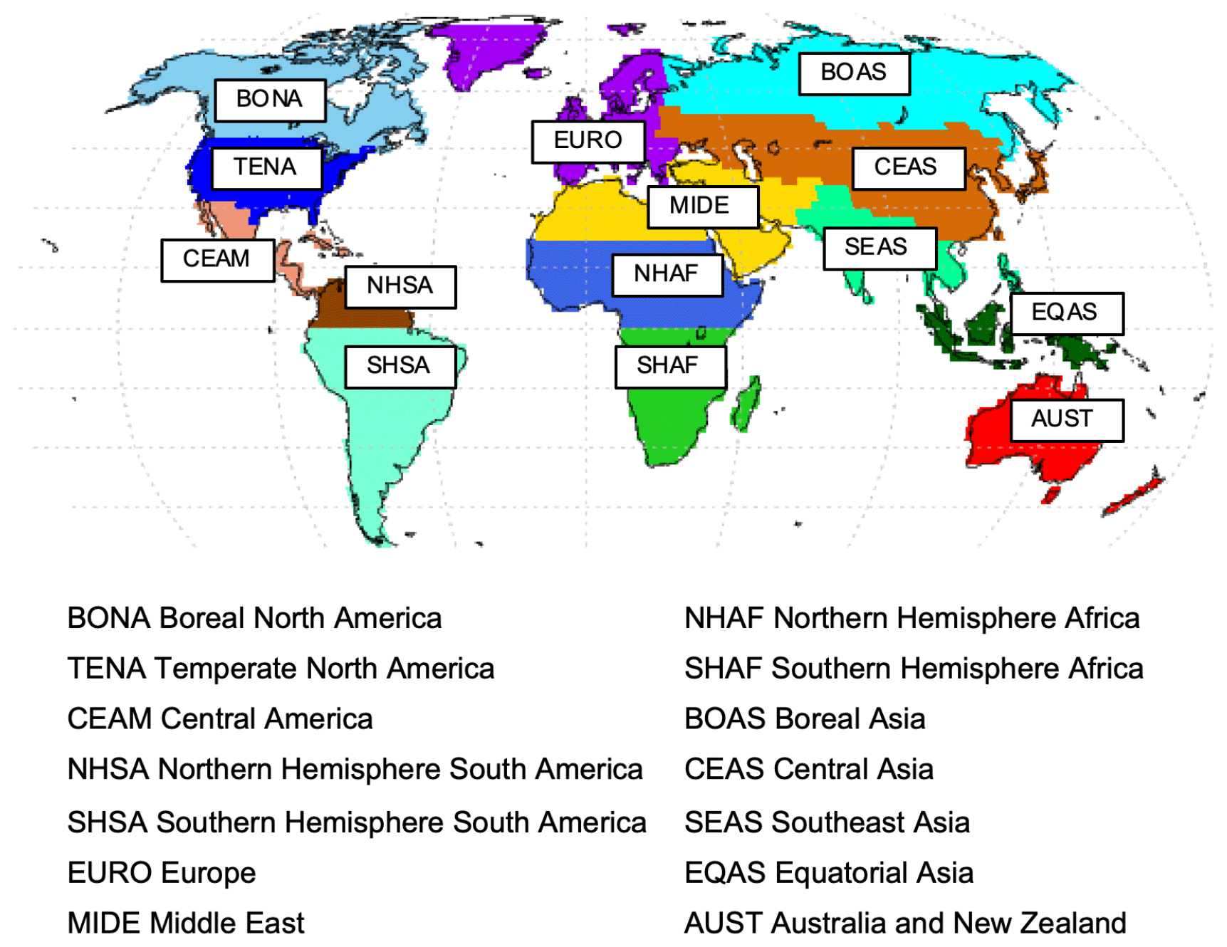
Figure 1 GFED (Global Fire Emissions Database) basis regions regridded to the resolution of ModelE2.1 of 2^∘ in latitude by 2.5^∘ in longitude.

BB can exist when three conditions are met: fuel is available, fuel is combustible, and ignition sources are present (Schoennagel et al., 2004). The coincidence of these conditions is seasonal, making open BB an inherently seasonal phenomenon. The peak month and duration of fire season are coupled to the seasonal cycle in precipitation, especially in the tropics (Giglio et al., 2006; Hantson et al., 2017). Precipitation and fire activity are sensitive to natural modes of variability like El Niño–Southern Oscillation (ENSO). In particular, the Southern Hemisphere BB activity is strongly coupled to ENSO (Buchholz et al., 2018). During an El Niño year, regional BB emissions can be up to 2 times higher than their regional average level, due to increased fire activity in tropical rainforests (van der Werf, 2004; Andela and Van Der Werf, 2014; Field et al., 2016; Whitburn et al., 2016).

Forest fires are ignited on purpose, as part of forest management practices (Ryan et al., 2013); ignited by accident, as a byproduct of the expansion of urban life to the wildland interface (Moritz et al., 2014; Fischer et al., 2016; Radeloff et al., 2018); or ignited by lightning (Díaz-Avalos et al., 2001). Thus, fire activity is highly coupled to trends in population density as increased population density at the wildland–urban interface (WUI) increases the probability of fire (Radeloff et al., 2018), while land abandonment leads to shrub encroachment and fuels fire activity (Butsic et al., 2015).

Although BB emissions have high spatiotemporal variability, their impact on atmospheric composition is significant (Crutzen et al., 1979; Seiler and Crutzen, 1980; Crutzen and Andreae, 1990). BB emissions impact air quality (Johnston et al., 2012, 2014, 2016; Bauer et al., 2019) and climate (Ward et al., 2012; Lasslop et al., 2019). Emitted pollutants include ozone precursors like methane (∼49 Tg a⁻¹), carbon monoxide (∼820 Tg a⁻¹), and NO_x (mostly emitted as NO, ∼19 Tg a⁻¹) (Andreae, 2019); the latter two are also deleterious for health on their own. In addition to gaseous pollutants, BB emits particulate matter (a total of ∼85 Tg a⁻¹) like primary emitted black carbon (∼5 Tg a⁻¹) and organic carbon (∼36 Tg a⁻¹), as well as precursors of brown carbon and secondary organic and inorganic aerosols like non-methane volatile organic compounds (NMVOCs, ∼58 Tg a⁻¹), ammonia (∼9.9 Tg a⁻¹), sulfur dioxide (∼6 Tg a⁻¹), and NO_x (Andreae, 2019). Exposure to these pollutants at high concentrations or for a long period of time can compromise the cardiorespiratory system and lead to death (Lelieveld et al., 2015). These pollutants, along with BB-emitted greenhouse gases (GHGs) like carbon dioxide (CO₂; ∼13 900 Tg a⁻¹) and nitrous oxide (N₂O; ∼1.38 Tg a⁻¹), interact with radiation (directly and indirectly). Fires are a net source of carbon dioxide only where vegetation regrowth is inhibited, i.e., in deforested areas; otherwise, BB is not viewed as a source of CO₂ but as “fast respiration” (van der Werf et al., 2017). Absorbing black and brown carbon (Lack et al., 2012; Lack and Langridge, 2013; Laskin et al., 2015) and reflecting primary and secondary organic and inorganic aerosols interact with solar radiation directly by scattering and absorbing radiation and indirectly by modifying clouds. The radiative properties of particles and their hygroscopicity are also influenced by their mixing state (Bauer and Menon, 2012). For example, when black carbon (BC) is coated it becomes even more absorbing per unit mass (Bond and Bergstrom, 2006). There is evidence that smoke plumes can suppress or invigorate precipitation (Feingold et al., 2001; Andreae et al., 2004; Tosca et al., 2015). Aerosols impact cloud height and cover by modifying the heat profile of the atmosphere and increasing the number of cloud condensation nuclei. There are large uncertainties associated with aerosols' impact on climate. Modeling studies suggest that the aerosol effects from BB emissions overrides the BB-GHG effect to a net negative radiative forcing (Mao et al., 2013), with the indirect effect of clouds dominating the forcing (Ward et al., 2012). The present-day BB forcing is estimated at −0.5–$(-\mathrm{0.1})\pm \mathrm{0.05}$ W m⁻² (Ward et al., 2012; Mao et al., 2013; Jiang et al., 2016; Landry and Matthews, 2016; Lasslop et al., 2019).

The quantification of speciated BB emissions is challenging due to the fact that no one fire is the same as another (Ito and Penner, 2005). The composition of the resulting smoke plume depends on the fuel type, burning conditions (i.e., flaming or smoldering), fuel consumption, and on background chemistry. More complete combustion has a higher fraction of oxidized species (e.g., CO₂ and NO_x), while smoldering fires release more reduced species (e.g., CO, NH₃, NMVOCs). Globally, most fire emissions occur during the active phase of the fire, with peat fires as the main exception (Andreae, 2019). Thus, emissions in different regions contribute different amounts of pollutants; Indonesia, for example, is responsible for 8 % of global carbon BB emissions but 23 % of methane BB emissions (van der Werf et al., 2017). Emissions are sensitive to season and region. Even within one region, like a boreal forest, emissions from crown fires differ from those from ground fires. The amount of fuel consumed by a fire is highly variable and depends on fuel load, density, moisture, vegetation type, and on environmental factors such as wind speed, soil moisture, and soil composition. Additional challenges relate to external forcing such as insect herbivory, mammal grazing, and anthropogenic land fragmentation and deforestation (Schultz et al., 2008). The quantification of BB emissions has an even bigger importance during preindustrial times, where fire emission are identified as the largest source of uncertainty for aerosol loading in Earth system models (Hamilton et al., 2018). BB emissions are a key quantity needed for quantifying the unperturbed-from-humans background conditions of the atmosphere (Carslaw et al., 2013).

Traditionally, fires are included in climate models using emission inventories (Lamarque et al., 2010; van der Werf et al., 2010, 2017; van Marle et al., 2017). Some models have the ability to simulate BB emissions interactively with a varying level of complexity (Thonicke et al., 2001; Arora and Boer, 2005; Pechony and Shindell, 2009; Li et al., 2012; Lasslop et al., 2014; Hantson et al., 2016; Mangeon et al., 2016; Rabin et al., 2017; Zou et al., 2019). On the one end of the spectrum, there are statistically based models and on the other end there are detailed empirical and physical process-based models. Statistical models are skilled at making predictions based on present-day relationships between climate and fire (their training data). Process-based models encapsulate the complex feedbacks within the climate system at various levels. They combine physical processes such as fuel condition, cloud-to-ground lightning ignitions, and wind-driven fire expansion. The most sophisticated models are coupled to dynamic global vegetation models (DGVMs) and directly connect fire–Earth-system interactions through fuel consumption (e.g., LPJ-GUESS-GlobFIRM, LPJ-GUESS-SIMFIRE-BLAZE; Smith et al., 2001, 2014; Lindeskog et al., 2013; and MC-Fire; Bachelet et al., 2015; Sheehan et al., 2015). Some models also include simplified empirical relationships of anthropogenic ignition and suppression, which, at present, are not understood in a dynamic process level. State-of-the-art process-based fire models are well equipped to study the feedbacks between the climate system and fires (Hantson et al., 2016). However, there is indication that they lack accurate predictive capabilities, as they only partly capture trends in present-day observations. For example, satellite products show a global decrease in burned area from about 500 Mha a⁻¹ in 1997 to 400 Mha a⁻¹ in 2013, a trend which fire models do not capture (Andela et al., 2017). This trend is mostly driven by land fragmentation and grazing practices over African savanna, highlighting the challenge of fire models to account for the combined changes in climate, vegetation, and socioeconomic drivers (Forkel et al., 2019). Though less accurate than observational datasets, when trying to simulate individual fire events, fire models provide the unique advantage of linking the atmosphere, biosphere, and hydrosphere in a consistent way, which is a crucial step when studying Earth system interactions. They are also able to predict fire during climate periods for which we have no observational data available (e.g., preindustrial and future).

In this paper we present a new global fire module, pyrE, based on an improved scheme of Pechony and Shindell (2009, 2010) with new capabilities. pyrE is a process-based module, as it includes the two basic parameters of fuel availability and combustibility, which are used to calculate active fires. It utilizes empirical relationships with population density to account for the anthropogenic impact on fire ignition and suppression. However, unlike most fire models where fire suppression is applied uniformly across all regions (Rabin et al., 2017), in pyrE fire suppression depends both on population density and region. Additionally, pyrE uses active fires to derive emissions in contrast to other fire models that use BA. The fire module is part of the NASA GISS ModelE Earth system model, ModelE2.1 (an updated version based on Schmidt et al., 2014), and is described below.

2 Model description

pyrE, from the Greek word for fire (pyr, πυρ), is a global fire module within GISS ModelE. It incorporates the active fire parameterization of Pechony and Shindell (2009, 2010), with the addition of fire spread and BA, following the Community Land Model's (CLM) approach (Li et al., 2012). The module is a collection of physical processes like flammability, natural ignition, fire spread, and fire emissions and empirical processes that include accidental ignition and suppression (Fig. 2). The climate model input required includes surface temperature, surface relative humidity (RH), precipitation, surface wind speed, vegetation density and type, cloud-to-ground (CG) lightning frequency, and population density. Like many fire modules, it lacks explicit intentional ignition (e.g., crop, deforestation) and peat fires.

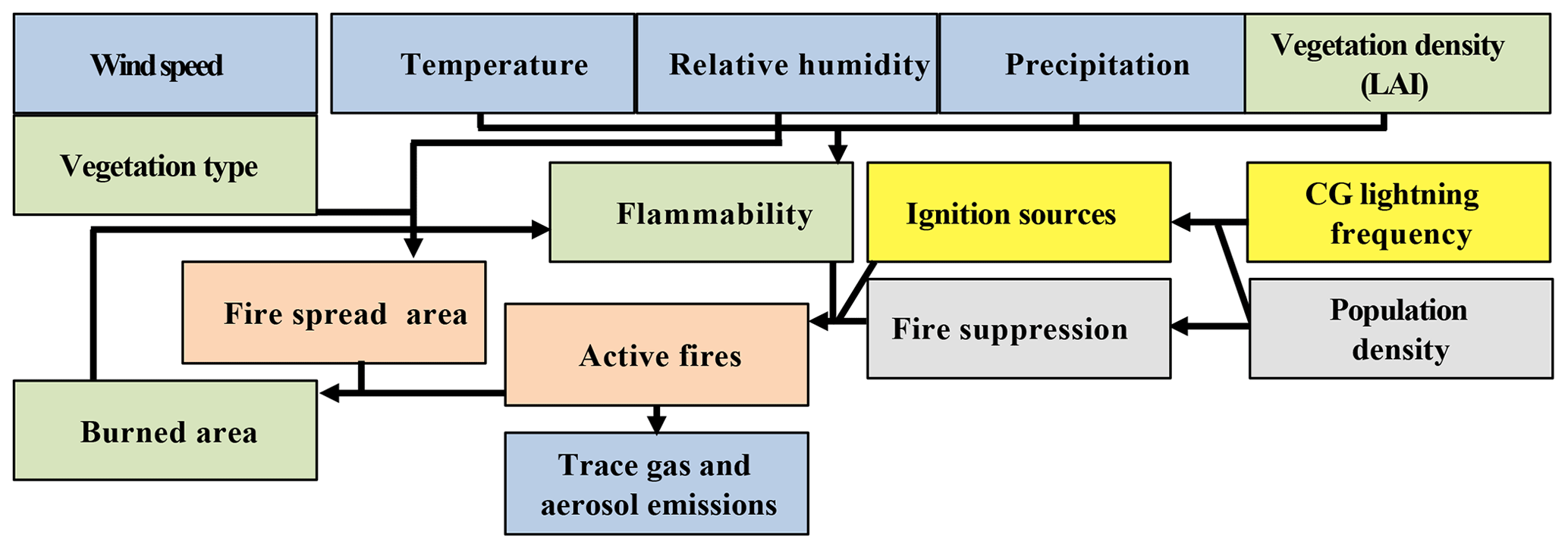
Figure 2 Structure of the fire parameterization of pyrE. Processes related to atmospheric properties are in blue, surface properties are in green, ignition and suppression are in yellow and gray, and fire properties are in red.

2.1 Flammability

Flammability is a parameter that indicates conditions favorable for fire occurrence (Pechony and Shindell, 2009, 2010). It is a unitless number that ranges between zero and one, and it is calculated using vapor pressure deficit (VPD), monthly accumulated precipitation, and vegetation density (VD).

VPD, an indicator of drought (Seager et al., 2015; Williams et al., 2015), is calculated via the Goff–Gratch equation (Goff and Gratch, 1946; Goff, 1957) using the saturation vapor pressure (e_s) and surface relative humidity (RH):

$$\begin{array}{}\text{(1)}& \mathrm{VPD}=e_{\mathrm{s}}\left(\mathrm{1}-{\displaystyle \frac{\mathrm{RH}}{\mathrm{100}}}\right),\end{array}$$

where e_st=1013.245 mbar is the saturation vapor pressure at the boiling point of water and e_s=e_st10^Z(T) depends on temperature (T),

$$\begin{array}{}\text{(2)}& \begin{array}{rl}Z\left(T\right)=& a\left({\displaystyle \frac{T_{\mathrm{s}}}{T}}-\mathrm{1}\right)+b\cdot \log \left({\displaystyle \frac{T_{\mathrm{s}}}{T}}\right)+c\left({\mathrm{10}}^{d\left(\mathrm{1}-\frac{T_{\mathrm{s}}}{T}\right)}-\mathrm{1}\right)\\ & +f\left({\mathrm{10}}^{h\left(\frac{T_{\mathrm{s}}}{T}-\mathrm{1}\right)}-\mathrm{1}\right),\end{array}\end{array}$$

with the following coefficients: $a=-\mathrm{7.90298}$; b=5.02808; $c=-\mathrm{1.3816}\times {\mathrm{10}}^{-\mathrm{7}}$; d=11.344; $f=\mathrm{8.1328}\times {\mathrm{10}}^{-\mathrm{3}}$; $h=-\mathrm{3.49149}$ (Goff and Gratch, 1946); and T_s=373.16 K (water boiling point temperature).

The precipitation dependence of flammability is in the form of an inverse exponential (Following Keetch and Byram, 1968):

$$\begin{array}{}\text{(3)}& f\left(R\right)=\exp \left(-c_{R}R\right),\end{array}$$

where R is the surface rain rate in millimeters per day, and c_R=2 (d mm⁻¹) is an empirical constant (Pechony and Shindell, 2009).

Vegetation density (VD) is taken as the normalized leaf area index (LAI) in the land fraction of a grid cell, varying between 0 for no vegetation and 1 for dense vegetation.

We modified the original calculation proposed by Pechony and Shindell (2009) by calculating flammability only for the fraction of the model's grid cell that is not burned from previous fires. The flammability F at a time step t in a grid cell (i, j) is

$$\begin{array}{}\text{(4)}& \begin{array}{rl}F\left(t\right)=& {\mathrm{10}}^{Z\left(T{\left(t\right)}_{i,j}\right)}\left(\mathrm{1}-{\displaystyle \frac{\mathrm{RH}{\left(t\right)}_{i,j}}{\mathrm{100}}}\right)\mathrm{VD}{\left(t\right)}_{i,j}\\ & \left(\mathrm{1}-{\displaystyle \frac{\mathrm{BA}{\left(t\right)}_{ij,}}{L{A}_{i,j}}}\right)\exp \left(-c_{R}R{\left(t\right)}_{i,j}\right),\end{array}\end{array}$$

where LA_i,j is the total land area (LA) in the grid cell (i,j).

2.2 Ignition

Natural and anthropogenic ignition varies in space and time and is necessary for the calculation of active fires. If ignition is zero, the resulting number of active fires will be zero, independent of flammability. Natural ignition is in the form of cloud-to-ground lightning frequency, which is interactively calculated in ModelE2.1 (Price and Rind, 1992, 1993). The parameterization of anthropogenic ignition follows Venevsky et al. (2002) and is based on the assumption that in sparsely populated regions people interact more with the natural environment, thus increasing the potential for ignition. The parameterization uses population density data and empirical scaling factors, as described by Pechony and Shindell (2009), and does not include intentional ignition. The number of anthropogenic accidental ignitions per square kilometer per month is

$$\begin{array}{}\text{(5)}& I_{\mathrm{A}}=k\left(\mathrm{PD}\right)\mathrm{PD}\mathit{\alpha },\end{array}$$

where PD is the population density; $k\left(\mathrm{PD}\right)=\mathrm{6.8}{\mathrm{PD}}^{-\mathrm{0.6}}$ represents the varying anthropogenic ignition potentials as a function of population density; and α=0.03 is the number of potential ignitions per person per month. Coefficients are taken following Pechony and Shindell (2009) and Mangeon et al. (2016), which utilized correlation calculations done by Venevsky et al. (2002).

2.3 Suppression

A first-order approximation of the impact of population density on explicit fire suppression was proposed by Pechony and Shindell (2009). According to that parameterization, more fires are suppressed in densely populated areas compared to sparsely populated areas, regardless of ignition source. Specifically, suppression varies from 5 % to 95 % of fires. However, fire management is a region-specific practice, which depends on cultural norms and economic capabilities. For example, fire suppression in the United States of America (USA) is a common practice (Parisien and Moritz, 2009; Marlon et al., 2012), while active fire suppression in most parts of Africa is not commonly practiced. Most fire suppression in Africa is an indirect byproduct of changes in land surface properties through grazing and fragmentation (Archibald, 2016). Hence, we modified the simplistic approach suggested by Pechony and Shindell (2009), guided by the results presented in Sect. 5.1.1, to better match with observed fire activity at specific regions. Our initial analysis showed that with the original Pechony and Shindell (2009) suppression scheme fire activity is overestimated in the TENA and Middle East (MIDE) regions, while being underestimated in NHAF and SHAF. Following these initial results, a series of sensitivity simulations were conducted with varying values of suppression coefficients. The final values were chosen in a heuristic manner that improved the simulations yet did not over-fit them to the observations, similarly to Pechony and Shindell (2009) and other fire parameterization, due to the lack of appropriate global data.

We use the complement of the fraction of suppressed fires that is the fraction of non-suppressed fires, f_NS:

$$\begin{array}{}\text{(6)}& f_{\mathrm{NS}}=\left\{\begin{array}{ll}\mathrm{0.2}\exp (-\mathrm{0.05}\mathrm{PD}),& \text{USA and MIDE;}\\ \mathrm{1},& \text{Africa;}\\ \mathrm{0.05}+\mathrm{0.9}\exp (-\mathrm{0.05}\mathrm{PD}),& \text{elsewhere.}\end{array}\right.\end{array}$$

2.4 Active fires

Active fires are a key metric used to drive burned area and fire emissions in pyrE. The number of fires in a time step per square kilometer is calculated as the product of flammability, sum of natural and anthropogenic ignition, and suppression (Pechony and Shindell, 2009) (Fig. 2):

$$\begin{array}{}\text{(7)}& N_{\mathrm{fire}}{\left(t\right)}_{i,j}=F{\left(t\right)}_{i,j}\cdot \left(I_{\mathrm{N}}{\left(t\right)}_{i,j}+I_{\mathrm{A}}{\left(t\right)}_{i,j}\right)\cdot f_{\mathrm{NS}}{\left(t\right)}_{i,j}.\end{array}$$

2.5 Burned area (BA)

We adopted the process-based approach by Li et al. (2012) to calculate fire spread and burned area. The burned area in grid cell (i,j) at a model time step t is the product of active fires and the weighted average over plant functional types (PFTs) of the area burned by one fire:

$$\begin{array}{}\text{(8)}& {\mathrm{BA}}_{i,j}=N_{\mathrm{fire}}{\left(t\right)}_{i,j}\cdot \sum _v{a}_{i,j,v}\cdot f_{i,j,v},\end{array}$$

where $f_{i,j,v}$ is the fractional area covered by plant functional type v, and the burned area of a single fire $a_{i,j,v}$ is assumed to have an elliptical shape (Fig. 3). Wind speed, surface relative humidity, and vegetation type control the eccentricity of the ellipsoid that represents the burned area of a single fire (based on van Wagner, 1969):

$$\begin{array}{}\text{(9)}& a_{i,j,v}={\displaystyle \frac{\mathit{\pi }{\mathrm{ROS}}^{\mathrm{2}}{\mathit{\tau }}^{\mathrm{3}}}{\mathrm{4}\mathrm{LB}}}{\left(\mathrm{1}+{\displaystyle \frac{\mathrm{1}}{\mathrm{HB}}}\right)}^{\mathrm{2}},\end{array}$$

where ROS is the rate of fire spread, LB is the length-to-breadth ratio, and HB is the head-to-breadth ratio. The stronger the wind, the more eccentric the ellipse, i.e., the bigger the length-to-breadth ratio:

$$\begin{array}{}\text{(10)}& \mathrm{LB}=\mathrm{1}+\mathrm{10}\cdot \left(\mathrm{1}-\exp \left(-\mathrm{0.06}W\right)\right),\end{array}$$

where W is the surface wind speed (in m s⁻¹).

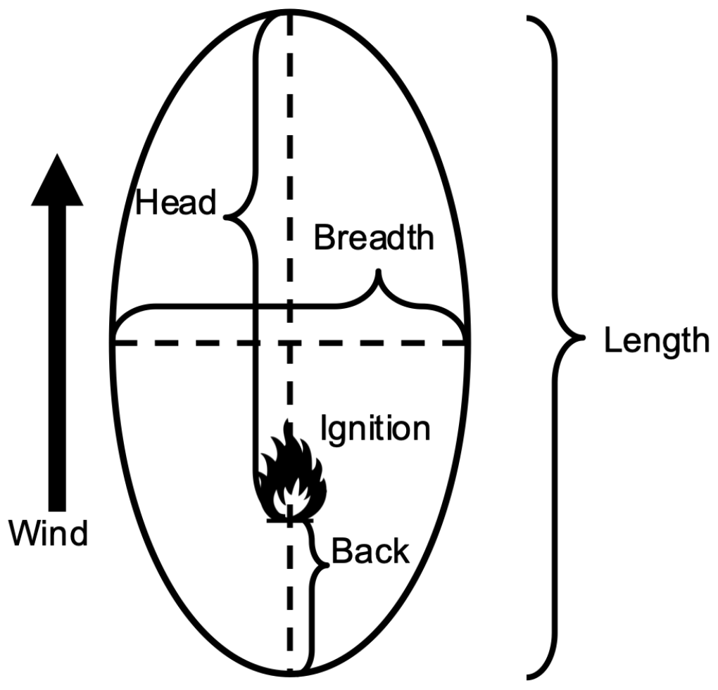
Figure 3 Approximation of a single fire spread. Based on van Wagner (1969) and Arora and Boer (2005).

Strong winds also increase the head-to-breath ratio, the ratio of the downwind spread compared to the upwind spread:

$$\begin{array}{}\text{(11)}& \mathrm{HB}={\displaystyle \frac{\mathrm{LB}+\sqrt{{\mathrm{LB}}^{\mathrm{2}}-\mathrm{1}}}{\mathrm{LB}-\sqrt{{\mathrm{LB}}^{\mathrm{2}}-\mathrm{1}}}}.\end{array}$$

The rate of spread (ROS) of a fire is a function of vegetation type, wind speed, and atmospheric and soil moisture:

$$\begin{array}{}\text{(12)}& \mathrm{ROS}={\mathrm{ROS}}_{max}\cdot gW\cdot f_{\mathrm{RH}}\cdot f_{\mathit{\theta }}.\end{array}$$

ROS_max is the maximum fire spread rate. Following Li et al. (2012), we set it to 0.2 m s⁻¹ for grasses, 0.17 m s⁻¹ for shrubs, 0.15 m s⁻¹ for needleleaf trees, and 0.11 m s⁻¹ for other trees. Li et al. (2012) estimated the fire spread coefficients to be on the lower range of observed ROS, but they are yet higher than the global value of 0.13 m s⁻¹ suggested by Arora and Boer (2005).

The limit of the fire spread is set by

$$\begin{array}{}\text{(13)}& gW={\displaystyle \frac{\mathrm{2}\mathrm{LB}}{\mathrm{1}+\frac{\mathrm{1}}{\mathrm{HB}}}}g,\end{array}$$

where

$$g\mathrm{0}={\displaystyle \frac{\mathrm{1}+{\mathrm{HB}}_{max}^{-\mathrm{1}}}{\mathrm{2}{\mathrm{LB}}_{max}}}\approx \mathrm{0.05}.$$

f_RH and f_θ are the dependencies of fire spread on RH and root zone soil moisture:

$$\begin{array}{}\text{(14)}& f_{\mathrm{RH}}=\left\{\begin{array}{cc}\mathrm{1},& \mathrm{RH}\le {\mathrm{RH}}_{\mathrm{low}};\\ \frac{{\mathrm{RH}}_{\mathrm{up}}-\mathrm{RH}}{{\mathrm{RH}}_{\mathrm{up}}-{\mathrm{RH}}_{\mathrm{low}}},& {\mathrm{RH}}_{\mathrm{low}}<\mathrm{RH}<{\mathrm{RH}}_{\mathrm{up}};\\ \mathrm{0},& \mathrm{RH}\ge {\mathrm{RH}}_{\mathrm{up}}.\end{array}\right.\end{array}$$

Following Li et al. (2012), we set RH_low=30 %, RH_up=70 %, and f_θ=0.5 as ModelE2.1 does not simulate prognostic root zone soil moisture.

2.6 Emissions

Trace-gas and aerosol emissions are generated during the active phase of the fire, and they are calculated as the product of the simulated active fires and emission factors (EF_s,v) and are a function of PFT (denoted by v) and chemical species (denoted by s). The use of active fires to derive emissions is driven by the extremely rudimentary representation of the terrestrial biosphere in ModelE, under which interactive fuel consumption cannot be calculated. The emissions per grid cell (i,j) of species s at a model time step t are calculated by

$$\begin{array}{}\text{(15)}& E_{i,j,s}\left(t\right)=N_{\mathrm{fire}}{\left(t\right)}_{i,j}\cdot \sum _v{\mathrm{EF}}_{s,v}\cdot f_{i,j,v},\end{array}$$

where $E_{i,j,s}\left(t\right)$ is the emissions flux rate (in kg m⁻² s⁻¹), N_fire(t)_i,j represent the number of active fires, EF_s,v represents the offline emission factors, and f_v is the fractional area of that PFT in the grid cell.

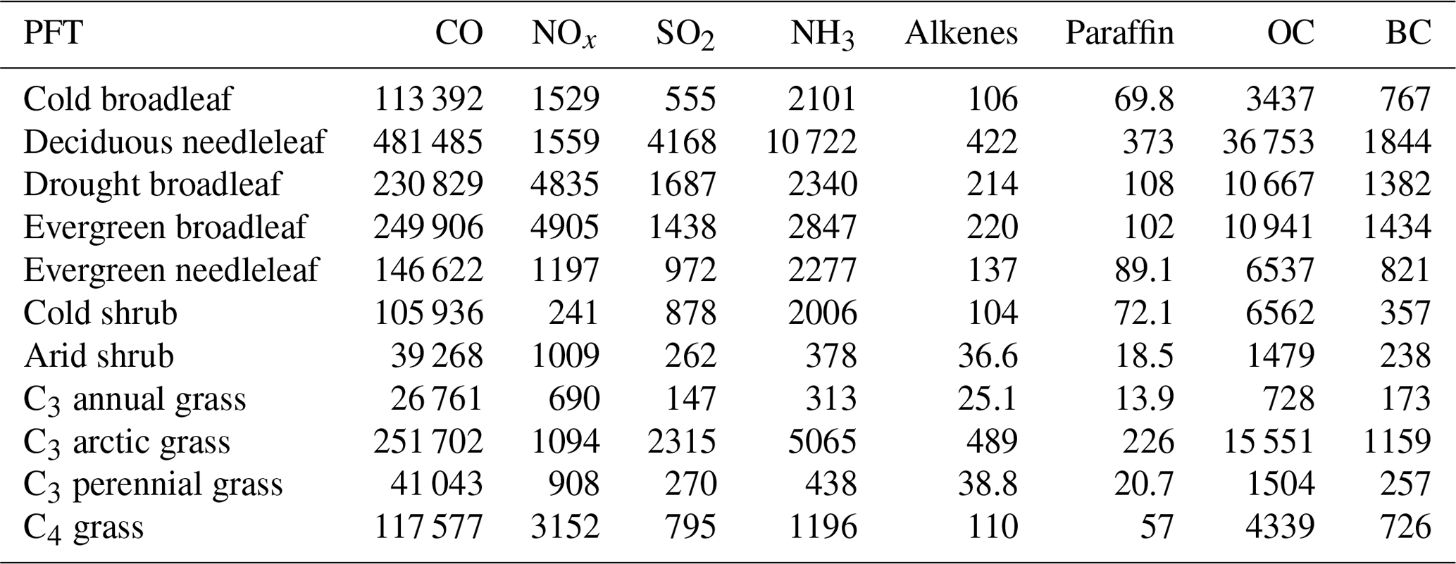
Emission factors describe the PFT-specific speciated mass (in kg) of the smoke, which is normalized per fire (Table 1). Emission factors were calculated offline using ModelE2.1 PFTs, annual mean global MODIS Terra fire count, and GFED4s emissions from the period of 2003–2009. Our technique, known as multivariate curve fitting, matched the emissions within the PFT fraction of the grid cell with the respective fire count. We correlated a time series of GFED4s emissions with a time series of MODIS fire count for each modeled PFT in a grid cell. Our settings included statistical (Poisson) weighting of the GFED4s emissions (1 over emissions) and a uniform initial estimate of 100 000 kg m⁻² s⁻¹ per fire per PFT. This calculation resulted in a specific emission factors per PFT (Table 1).

Table 1 Fire emission factors for the different plant functional types (PFTs) in ModelE2.1. Factors are in units of kilograms per fire per PFT in the grid cell. For organic carbon (OC) and black carbon (BC) units, kilograms is substituted with kilograms of carbon.

2.7 Implementation within ModelE

ModelE2.1 can be used with either GFED4s prescribed fire emissions or interactive pyrE emissions. The pyrE module generates emissions at every model time step with ESM-simulated (Earth system model) climate as a driver. Flammability is calculated only in the fraction of grid cells with natural vegetation. It is driven by the simulated surface RH, surface temperature, monthly accumulated precipitation, and LAI. LAI is calculated by Ent (Kim et al., 2015), which is the terrestrial biosphere model component of ModelE2.1 and is currently derived from 2005 MODIS LAI data (Tian et al., 2002a, b). Cloud-to-ground lightning, calculated by ModelE2.1, is used as the natural ignition source. Most ESMs have low skill in reproducing flash rate distributions (Murray, 2016), and the GISS model is no exception. A qualitative comparison with the World Wide Lightning Location Network (WWLN) (not presented here) showed that modeled cloud-to-ground lightning, which makes up only about 30 % of total lightning, is biased high in ModelE2.1. We decided to use a simple scaling factor of 0.1 in the calculation of natural ignition to better match observed flash rates, as improving the lightning parameterization is beyond the scope of this study.

All fire-related parameters like flammability, active fires, burned area, and fire emissions are recalculated in every model time step (30 min) with memory only of the burned area in the previous time step. We could not extend the “fire memory” past the previous time step due to limitations related to ModelE's terrestrial biosphere module. However, this is a reasonable application, given that the climate inputs we use for fire calculations such as monthly accumulated precipitation, surface RH, and temperature do not change significantly between each time step. The fire module's impact on the Earth system is currently only through interactive emissions. Albedo, carbon stocks, and LAI are not modified by pyrE.

The modeling approach presented in this paper provides a good reproduction of the seasonality compared to satellite retrievals (see “Results and discussion” section). However, the simulated magnitude of active fires and burned area was too small compared to satellite retrievals and required the use of a scaling factor, which is a common practice among other fire models (Pfeiffer et al., 2013; Hantson et al., 2016; Mangeon et al., 2016; Zou et al., 2019). To calibrate the global modeled active fires to MODIS retrievals, we used a global scaling factor of 30 for all active fires. A similar approach was taken by Pechony and Shindell (2009). We scaled burned area by a factor of 250 to reach the magnitude of GFED4s. Nevertheless, even with this large correction factor, burned area, which accounts for a small fraction of the grid cell that is able to burn, has a very minor impact on fire activity and fire emissions as its only impact to fire activity is through flammability.

3 Model configuration

We used ModelE2.1 with a spatial resolution of 2^∘ in latitude by 2.5^∘ in longitude, 40 vertical layers, and a model top at 0.1 hPa. The vegetation component of ModelE2.1 is the Ent Terrestrial Biosphere Model (Ent TBM), which is coupled with the land-use and land-cover data in the model (Kim et al., 2015). Ent prescribes leaf area index (LAI) for 14 plant functional types (presented in Table 1) derived from MODIS 2005 data (cover and biome types; Friedl et al., 2010; LAI; Tian et al., 2002a, b), historical crop cover (Pongratz et al., 2008), and vegetation heights from Simard et al. (2011).

In this study we show results from runs of ModelE2.1 coupled to the aerosol microphysical scheme MATRIX (Multiconfiguration Aerosol TRacker of mIXing state) (Bauer et al., 2008). MATRIX simulates aerosol formation, condensation, and coagulation; calculates the size distribution of aerosols; and tracks their mixing state. Sea salt, dust, and dimethyl sulfide (DMS) emissions were calculated interactively, driven by the simulated climate, while other natural and anthropogenic fluxes, except for fires, were prescribed from the CEDS (Community Emissions Data System) inventory (Hoesly et al., 2018).

In the following, we will present a simulation with pyrE turned on, generating interactive fire emissions, and a simulation with pyrE turned off, using prescribed 2005 climatological (interpolated 2000–2010) GFED4s emissions instead. Also, we will discuss sensitivity studies using two simulations where pyrE generates interactive fire emissions but suppression is changed from a global parameterization to a regional one. Prescribed climatological monthly varying mean (1996–2004) sea surface temperature and sea ice thickness and extent were used as boundary conditions (Rayner et al., 2003).

4 Dataset

Most of the data below are based on a composite of level-3 Aqua and Terra Moderate Resolution Imaging Spectroradiometer (MODIS) Collection 5.1 data (Giglio et al., 2003b; Giglio, 2013) unless otherwise stated. Aqua and Terra are Sun-synchronous near-polar orbiting satellites with a global continuous record of more than 15 years; Aqua was launched in May 2002 and Terra in December 1999. Aqua's overpass times are 01:30 and 13:30 LT (local time) and Terra's overpass times are 10:30 and 22:30 LT, and their period is between 1 and 2 d. All reference data used in this study are interpolated and regridded to the resolution of ModelE2.1.

4.1 Population density

Gridded population density (PD) that drives both anthropogenic ignition and fire suppression is based on historical data for years prior to 2010 (Klein Goldewijk et al., 2010). PD has a time resolution of 10 years and is interpolated in between.

4.2 Fire count

To detect fires, MODIS uses brightness temperatures (thermal anomaly) derived from two channels (Justice et al., 2002; Giglio et al., 2006). In our study we used the monthly cloud-corrected fire count (CloudCorrFirePix) climate model grid data (MYD14CMH, MOD14CMH). One single fire might include multiple fire pixels. The spatial resolution of the data is 0.5^∘. Static, persistent hot spots are excluded from this product (Giglio, 2013). Because of its nonuniform spatial and temporal sampling, raw MODIS data are biased high at high latitudes (Giglio et al., 2003a, 2006). The product we used is corrected for the multiple satellite overpasses, the missing data, and variable cloud cover. Cloud cover hinders MODIS retrievals. The active fires in the product we used are normalized to the fraction of cloud cover in a pixel. In highly cloudy pixels, the product is set to zero. The local time of retrieval matters for fire detection, as fires are driven by the daily cycle of solar heating. The largest number of active fires is detected during daytime, with an order of magnitude difference between daytime detections and nighttime detections (Ichoku et al., 2008). Thus, differences are evident between the Aqua and Terra retrievals. This motivated us to use data from the two satellites in our analysis. We calculate and utilize climatological monthly means from the period 2003–2016.

4.3 Burned area

We used burned area from the Global Fire Emissions Database (GFED) version 4s that includes small fires (van der Werf et al., 2010, 2017; Randerson et al., 2012; Giglio et al., 2013). The GFED4s inventory is based on multisensor MODIS data, involving both reflectance and thermal anomaly measurements from Aqua and Terra. Retrievals must be free from cloud contamination and free from active fires within the 500 m MODIS grid cell. First, to generate the GFED4s data, MODIS burned area collection 5.1 data (MCD64A1 product) are aggregated to a 0.25^∘ grid. Then, burned area from small fires is added. The burned area of small fires is statistically estimated using active fires detected by MODIS (a composite of both Aqua and Terra). In this study we use climatological monthly means of burned area from the period 2003–2016.

4.4 Biomass burning emission inventory

GFED4s emissions are derived from the multiplication of burned area and fuel consumption (van der Werf et al., 2010, 2017). As such, they have the same spatial and temporal resolution as burned area (0.25^∘ by 0.25^∘ and a month). Fuel consumption is calculated using an estimation of fuel loss and combustion completeness, which are calculated using MODIS-based metrics such as differences in normalized burned area (dNBR), normalized difference vegetation index (NDVI), and land surface temperature (LST). The satellite-based data are used as input to the Carnegie–Ames–Stanford Approach (CASA) biogeochemical model (Randerson et al., 1996) to calculate the dry matter burned. Then, emission factors (Andreae and Merlet, 2001; Akagi et al., 2011) are applied to convert the dry matter burned to PFT-specific speciated gas and aerosol phase emissions. Kaiser et al. (2012) and Pan et al. (2020) showed that there are regional biases in older and current versions of GFED, being especially biased low in the Southern Hemisphere compared to AERONET (AErosol RObotic NETwork) aerosol optical depth (AOD). In order to eliminate the strong interannual BB variability, our analysis used GFED4s mean climatological data for 2000–2010.

4.5 Fire regions

The analysis we present below is based on the widely used fire regions (Fig. 1) as defined by GFED (Giglio et al., 2006; van der Werf et al., 2006). The regions are defined based on climate and fire regimes, and they are widely used as basis regions for global fire studies.

4.6 Aerosol optical depth

The impact of fire emissions on atmospheric composition is investigated by comparing monthly Aqua and Terra MODIS retrievals of AOD at 550 nm (Remer et al., 2005; Platnick et al., 2015). AOD describes the entire atmospheric column-integrated extinction of aerosols. MODIS AOD data are a useful tool in the study of simulated BB plumes (Voulgarakis and Field, 2015; Johnson et al., 2016; Bauer et al., 2019). The AOD data we used have a 1^∘ spatial resolution. The monthly-mean data (MYD08_M3 and MOD08_M3 products) have been averaged over the period 2003–2007 to create monthly climatologies centered around the year 2005. The AOD product we use includes improvements made via the Dark Target algorithm (Kaufman et al., 1997), which was developed particularly for retrievals over dark, vegetated surfaces (Wei et al., 2019). However, the algorithm fails at retrieving valid AOD data over bright surfaces like desert areas (Levy et al., 2013), which we discard. Here we use collection 6.1 data.

5 Results and discussion

5.1 Fire activity

5.1.1 Regional suppression

First we want to demonstrate how the parameterization with regionally dependent fire suppression improves the simulation of fire activity compared to the original simplified global fire suppression proposed by Pechony and Shindell (2009) (Fig. 4). Our goal was to improve the fire parameterization in regions where the seasonality was captured in timing but not in magnitude. We propose regional modifications to Africa (NHAF, SHAF), a region that drives global fire activity, and had a distinct mismatch in active fires compared to satellite retrievals. Originally, over NHAF the fire seasonality was too flat, while over SHAF it matched MODIS Terra, but was orders of magnitude smaller than MODIS Aqua. Since fire suppression for open BB is not commonly practiced in rural Africa, eliminating it over NHAF and SHAF helped resolve the seasonal cycle (Fig. 4 and Eq. 6). The two other regions we modified are TENA and Middle East (MIDE). Over both of those regions the simulated fire seasonality was too strong. Increasing fire suppression over MIDE and TENA greatly improved our simulations compared to MODIS retrievals.

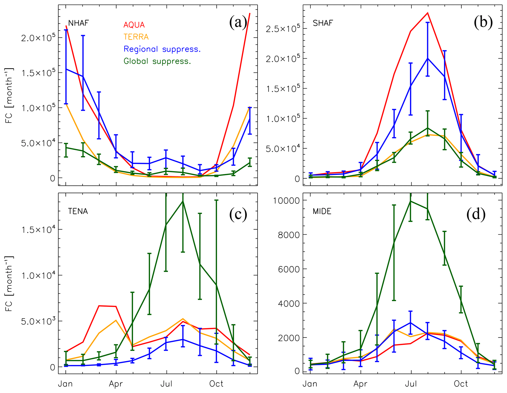
Figure 4 Seasonality of total active fires for NHAF (a), SHAF (b), TENA (c), and MIDE (d) observed by MODIS Aqua (red) and Terra (orange) and simulated with explicit regional suppression (blue) and generic global suppression parameterization (green) (Eq. 6). Error bars represent the range over 10-year climatological simulations. Note that TERRA and AQUA have different overpass times, and the model data presented here are monthly means. Also note the different scales in each panel.

The pyrE module is skilled at capturing the fire seasonality in regions identified by Forkel et al. (2017) as controlled by temperature and wetness (climate controls), like Southern Hemisphere South America (SHSA) (Fig. A1). However, there are regions that our parameterization does not simulate well, mainly due to the fact that the fire activity there is driven by land-use practices and intentional fire ignitions, which pyrE does not resolve. For example, in TENA we are missing the spring peak of agricultural fires. Similarly, over Europe and Boreal Asia (Fig. A1) we are missing the winter and spring fires associated with intentional ignition (Dwyer et al., 2000; Ganteaume et al., 2013). Other regions where the seasonality is not well captured, likely due to the fact that it is driven by intentional ignitions, include Central America, Northern Hemisphere South America, Central Asia, Southeast Asia, and Equatorial Asia. Over Australia, the model captures neither the magnitude nor the timing of the BB seasonality. This is in part due to the model's poor performance of the simulated cloud-to-ground lightning ignitions in that region (not shown).

In all simulations going forward we used the regional suppression scheme.

5.1.2 Daily cycle

We looked at the daily cycle of the active fires to see if it can explain the differences between Aqua, Terra, and the model. The monthly-mean fire count detected by Aqua and Terra is expected to be different due to their different overpass times. In Fig. 5, pyrE simulates a distinct daily cycle in active fires in different locations. The simulated daily cycle is most strongly controlled by the simulated daily cycle in flammability (not presented here), matching the daily solar cycle. pyrE's ability to resolve a daily cycle of fire activity highlights the dynamic nature of a process-based fire model.

Figure 5 Daily mean cycle in active fires (FC, blue line) and daily mean (black line) at four locations (Russia a, India b, Brazil c, Nigeria d) during the month of January. The daytime overpass times of Terra (10:30 LT) and Aqua (13:30 LT) are marked with a red star. Error bars represent the range during the month. Note the different scales in each panel.

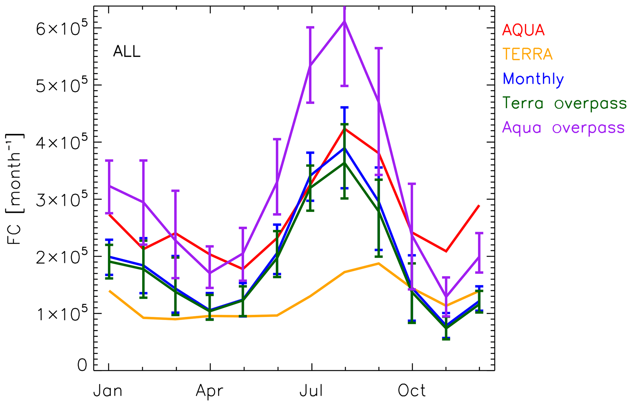
Figure 6 Global seasonality of total active fires (FC) by MODIS Aqua (red) and Terra (orange) and simulated by the model: monthly mean (blue), monthly mean sampled at the daytime Terra overpass time (green), and sampled at the daytime Aqua overpass time (purple). Error bars represent the 10-year range in the simulation.

Using 30 min simulation output, we sampled all surface grid cells at the daytime overpass time of MODIS Terra, 10:30 LT, and MODIS Aqua, 13:30 LT. We focused on the daytime overpass time of Terra and Aqua since about 95 % of active fire detections occur then (Ichoku et al., 2008). Our results in Figs. 6 and 7 indicate that, globally, simulated active fires sampled at daytime overpass times are biased high compared to MODIS retrievals from the respective satellite for much of the year. On a global annual mean, the active fires of the model sampled in daytime Terra overpass time are higher than MODIS Terra by 45 %, while the active fires of the model sampled in daytime Aqua overpass time are higher than MODIS Aqua by 13 %. However, this behavior differs by region and maximizes in NH sub-Saharan Africa and SH central Africa. The simulated fire activity is biased low compared to MODIS retrievals along the coast of west Africa, in eastern southeast Asia and Australia. When simulated monthly-mean active fire values are in the range of Terra and Aqua (Figs. 4, A1), they are in fact biased high, given the bias due to the overpass time of the satellite. Considering that the actual number of active fires is likely higher than the number retrieved by MODIS, as cloud contamination is decreasing its detection efficiency, it is conceivable that a model weakly biased high compared to the satellite retrievals is realistic. All results presented later were not sampled according to a satellite overpass time but instead were averaged over the whole length of the day.

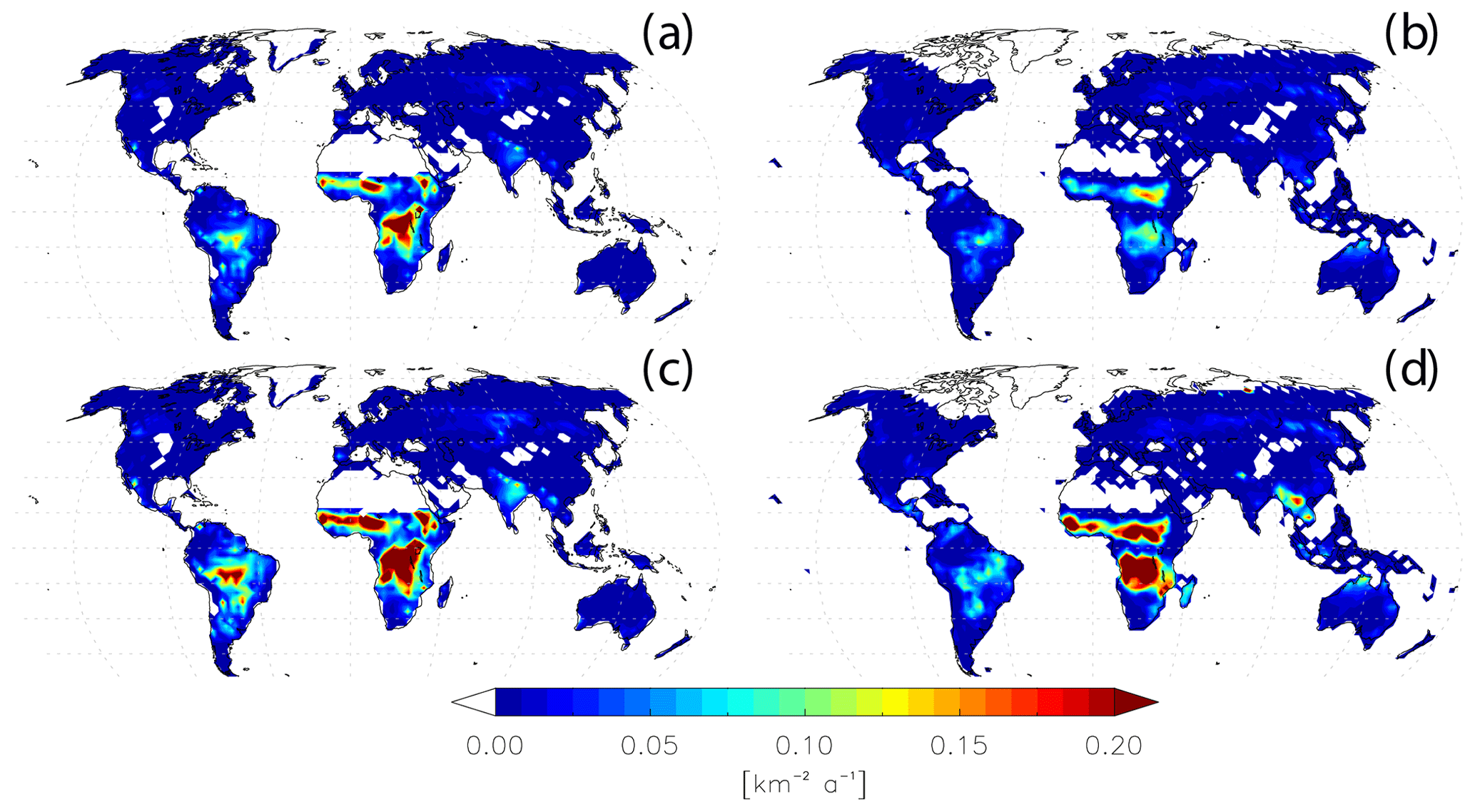
Figure 7 Annual mean model (a, c) and MODIS (b, d) active fires. Modeled annual mean is based on an ensemble of 10 simulations. Simulated fires sampled at the daytime Terra overpass time, 10:30 LT (a), and daytime Aqua overpass time, 13:30 LT (c). MODIS active fires are based on MODIS Terra (b) and MODIS Aqua (d) from 2003 to 2016.

5.2 Burned area

The simulated burned area is biased low compared to the GFED4s inventory (Figs. 8, A2). The total annual simulated burned area (10-year climatological mean) is 380 Mha, while GFED4s burned area (mean of 2003–2016) is 460 Mha. However, this behavior is region specific. The simulated burned area is lower compared to GFED4s over Northern Hemisphere Africa, particularly in November–December; over central and equatorial Asia; and over Australia. The simulated burned area (Figs. 8, A2) reflects the spatial distribution and seasonality of simulated active fires (Figs. 8, A1). GFED4s burned area and MODIS fire count do not always have the same seasonality, e.g., during October–December. During this season the satellite-retrieved fires produce a higher burned area relative to other seasons. The fire activity driving this behavior occurs in the NHAF savanna, and Northern Hemisphere South America. In those regions and times of the year the normalized mean bias of modeled burned area is at least twice the size of the normalized mean bias of active fires, e.g., in NHAF a bias of 6.5 for burned area and 1–3 for active fires, depending on the MODIS satellite. This implies that for every fire modeled in these regions and season a smaller area is simulated to burn compared to the reference datasets.

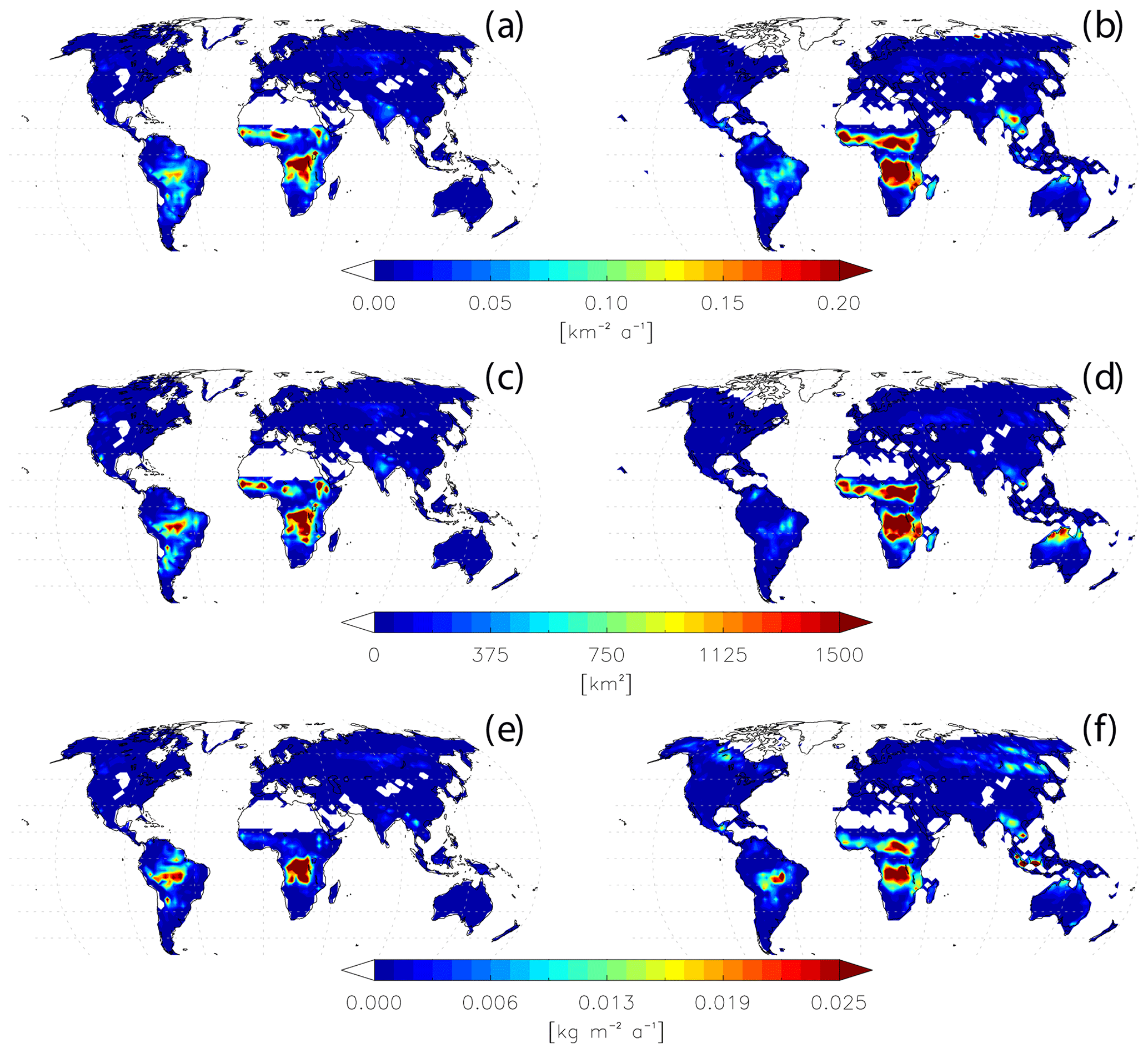
Figure 8 Annual mean model (a, c, e) and satellite-based (b, d, f) active fires (a, b), burned area (c, d), and CO emissions (e, f). Modeled annual mean is based on an ensemble of 10 simulations. Satellite-detected active fires are based on MODIS Aqua retrievals of 2003–2016, burned area is based on GFED4s inventory of 2003–2016, and CO emissions are based on climatological GFED4s emissions of 2000–2010.

Why is the burned area per fire relationship in simulations much weaker than it is in the reference datasets? Two contributing factors are prescribed PFT and simulated wind. The prescribed PFT distribution present in the model is rudimentary; it is comprised of 11 flammable vegetation types (Table 1). As for surface winds, the simulated wind patterns driving burned area are averaged over a coarse grid cell ($\mathrm{2}{}^{\circ }\times \mathrm{2.5}{}^{\circ }$). Simulated wind does not represent subgrid-scale processes and is not fueled by the fire's energy, which is likely contributing to an underestimation of the spread of burned area. However, though wind directly impacts burned area, it does not play a major role in the distribution of simulated fires, since burned area itself has a minor impact on fires through flammability due to its small percentage in a grid cell. At most, burned area reaches less than 18 % of the naturally vegetated fraction of a grid cell, and it is on average less than 1 %.

5.3 Emissions

Due to limitations in the current capabilities of the simulated terrestrial biosphere in ModelE, emissions are generated from active fires, similar to the approach by Pechony and Shindell (2009, 2010) and Pechony et al. (2013). The main source regions for fire emissions are NHAF, EQAS, SHSA, and SHAF. Emissions are well simulated over SHSA and SHAF (Figs. A3–A5), both in terms of timing of the seasonality and in magnitude. The main regions where simulated emissions are lower than GFED4s are NHAF and EQAS, mainly Indonesia (Figs. 8, A3–A5). However, more generally, simulated gaseous and particulate emissions are globally biased low compared to GFED4s emissions (Table 2). To a lesser degree, simulated fire emissions are also weaker compared to GFED4s in the boreal regions (Figs. A3–A5). The contribution from these regions to the global total is an order of magnitude smaller compared to the main source regions.

The weaker emissions compared to GFED4s are responding to the following inputs: offline emission factors, lack of crop and peat fires, LAI, and prescribed PFTs. The emission factors that generate fire emissions are derived using multivariate statistical analysis. Though we used 7 full years (2003–2009) of data to derive the factors, it might have generated biases in emissions. Areas that burn annually are properly sampled, but areas that have a fire cycle that is longer than 7 years might be biased high or low, depending on whether they were included in the training dataset or not. Also, crop and peat fires are not explicitly included in the simulated emissions, as intentional ignition is not parameterized in pyrE. Specifically, fires are not applied to the crop faction of a grid cell, and peat surfaces are not included in the PFTs. However, our method of deriving the offline emission factors uses MODIS fire count and GFED4s emissions, and it does not distinguish between intentional and accidental fires. Hence, intentional fires are indirectly accounted for in the global sum. However, this indirect inclusion of intentional fires does not necessarily add missing fire emissions in the correct locations. The LAI in Ent, ModelE's DGVM, is based on 2005 MODIS retrievals. Though we cannot estimate the role that the lack of interactive LAI plays, it is certainly not optimal, neither for fire activity simulation nor for fire emissions that are derived from active fires. Unlike simulated active fires, simulated fire emissions are strongly tied to the map of PFTs. The offline emission factors are based on prescribed PFTs, and the interactive emissions themselves are applied according to the subgrid PFT distribution. The prescribed PFT distribution present in the model might be different than reality, and those differences affect emissions. In the model, in areas where emissions are biased high compared to GFED4s, there is a high percentage (>50 %) of the following PFTs: evergreen broadleaf trees (Amazon, central Africa), cold broadleaf trees (northeast America, Europe), and drought broadleaf trees (central Africa and northern India). In EQAS, a region with biased low simulated emissions, close to 100 % of the prescribed PFTs is evergreen broadleaf trees, which in reality is replaced by crops. The biased low emissions in EQAS are very likely tied to the lack of prescribed peat PFT. In areas with biased low emissions, modeled PFTs are mainly (>50 %) C₄ grass (NHAF, Australia), deciduous needleleaf trees (boreal regions), and arid shrubs (Southern Africa, Australia).

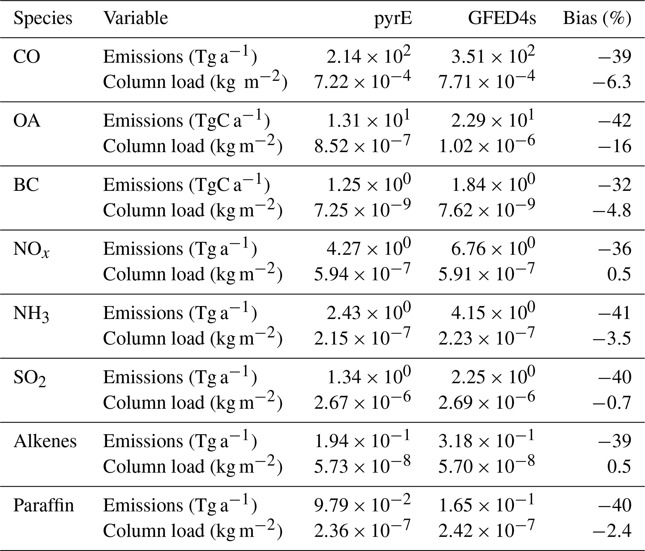
Table 2 Total fire emissions and global mean column loads of fire emitted species. Modeled annual emissions and column load means are based on an ensemble of 10 simulations. GFED4s emissions are based on a 2000–2010 climatological mean.

5.4 Composition

5.4.1 Column load

In order to quantify how the model skill changes with the inclusion of pyrE instead of prescribed emission inventory data in ModelE2.1, we compare a simulation with interactive fires to a simulation with prescribed BB sources. Though emissions are mostly biased low compared to GFED4s; this behavior is less evident in the column density (Fig. 9). For most BB emitted species, the simulation with interactive fires has lower column densities than the simulation with prescribed emissions (Table 2) with a bias ranging from −6.3 % to 0.5 % for gaseous species, −4.8 % for black carbon, and −16 % for organic aerosol (OA). However, the column densities are only partly driven by fire emissions, as those make up less than 35 % of total global emissions of CO, organic aerosol, and black carbon emissions. Non-emissions production-and-loss mechanisms also impact column densities. Having a weak global impact on composition does not imply that regional fires are not important.

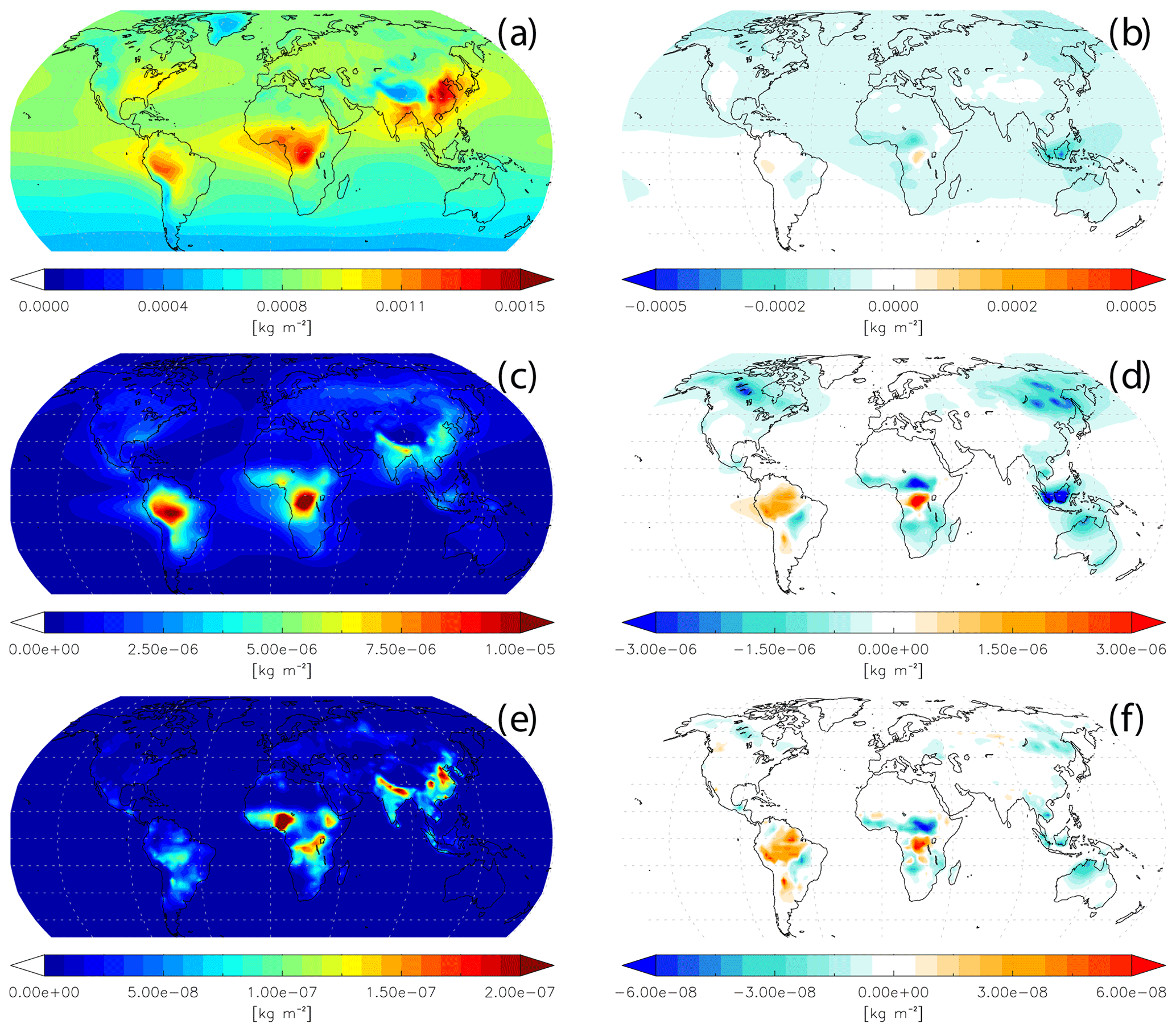
Figure 9 Modeled annual mean column density using pyrE fire emissions (a, c, e) and the difference in column densities with a simulation using offline GFED4s emissions (pyrE – GFED4s; b, d, f). CO (a, b), OA (c, d), and BC (e, f). Data based on an ensemble of 10 simulations.

The difference in column densities between the two simulations is greatest over northern sub-Saharan Africa, Indonesia, and the boreal regions. The behavior is region specific, and some regions like central Africa and Northern Hemisphere South America have higher column densities compared to the simulation with prescribed emissions. The differences between the two simulations are more prominent for organic aerosol than any of the other species (Fig. 9, Table 2), while the differences in the spatial distribution of CO are marginal.

5.4.2 Aerosol optical depth (AOD)

In Fig. 10 we compare climatologically simulated clear-sky AOD with MODIS AOD (Aqua) for January, April, July, and October. The conclusions from Terra products are similar to Aqua's and will not be presented here for brevity. In a regional perspective, simulated AOD is able to reproduce the seasonality and spatial distribution of MODIS-retrieved pollution over west and central Africa, east and southeast Asia, and the Arabian Sea. The simulations of ModelE2.1 have higher AOD compared to MODIS over the tropical eastern Pacific, which is an artifact due to the model's skill in simulating stratocumulus cloud decks, which have been improved in a newer version of the ESM (ModelE3).

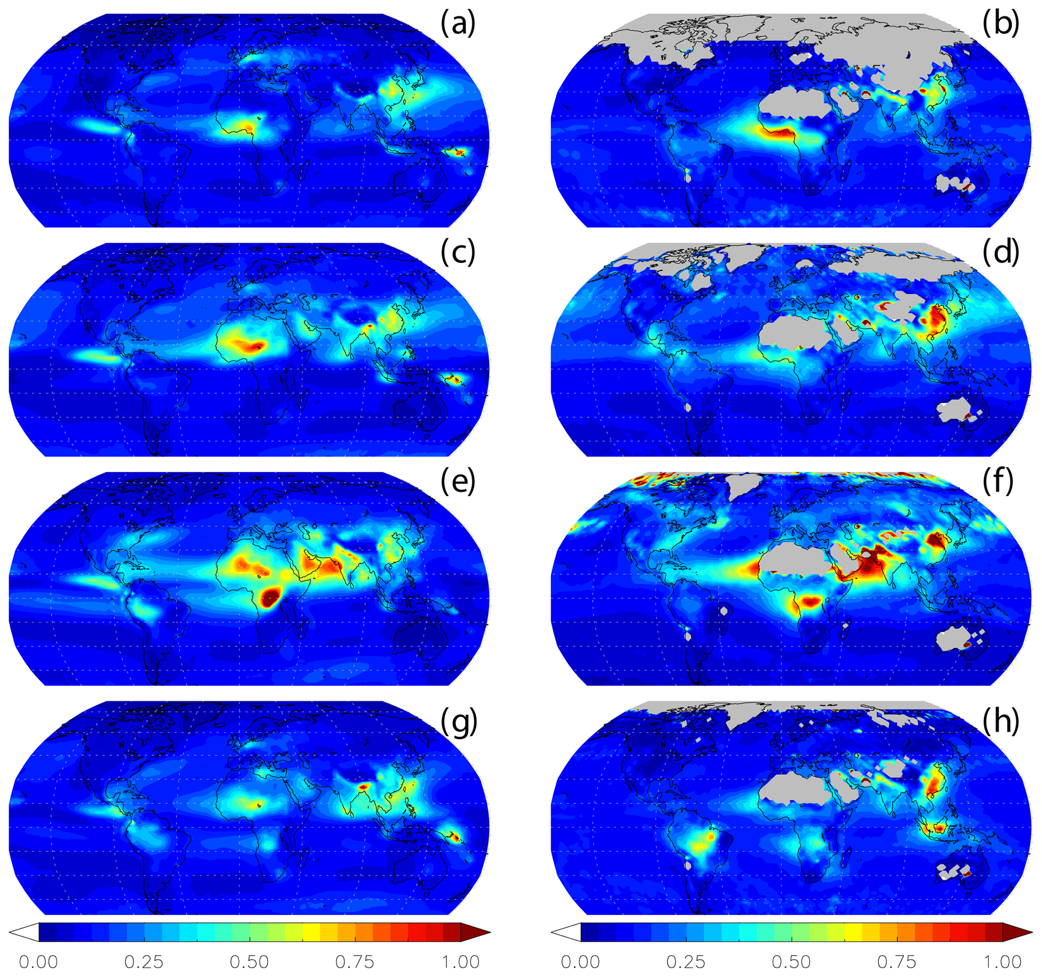
Figure 10 Monthly modeled clear-sky aerosol optical depth (AOD) simulated using pyrE fire emissions (left) and detected by Aqua MODIS (right): January (a, b), April (c, d), July (e, f), and October (g, h). Monthly-mean simulated AOD is based on an ensemble of 10 simulations, and climatologically monthly MODIS AOD is based on 2003–2007 data. Missing MODIS data are shaded in light gray.

Model performance as a function of interactive versus offline fire emissions is similar in terms of AOD (Fig. 11). Both simulations have persistently lower (0 %–30 %) AODs over central Africa and central South America compared to MODIS. The locations with an outstanding difference in performance between the simulations are in central sub-Saharan Africa in January and July and over a small area in Indonesia (Kalimantan) during October. In January over central sub-Saharan Africa the simulation with pyrE has AOD values (NHAF regional mean AOD of 0.26) closer to MODIS (NHAF regional mean AOD of 0.2) than a simulation with prescribed fire emissions (NHAF regional mean AOD of 0.33), while in July it is the simulation with pyrE (NHAF regional mean AOD of 0.53) that is more biased high than the prescribed one (NHAF regional mean AOD of 0.46). Over EQAS in October the simulation with prescribed fires has an AOD of ∼0.28, while the simulation with pyrE has an AOD of ∼0.18. AOD in this region is sensitive to peat fires, which are not included in ModelE, thus strongly impacting pyrE's results. Globally, mean AOD simulated with interactive fire emissions is 0.142, while mean AOD simulated with prescribed fire emissions is 0.146. The fact that pyrE has a marginal performance in climatological runs when compared against a simulation with the more accurate offline emissions is a strong indication that it is a robust module that can be used with confidence at time periods when offline emissions are not available.

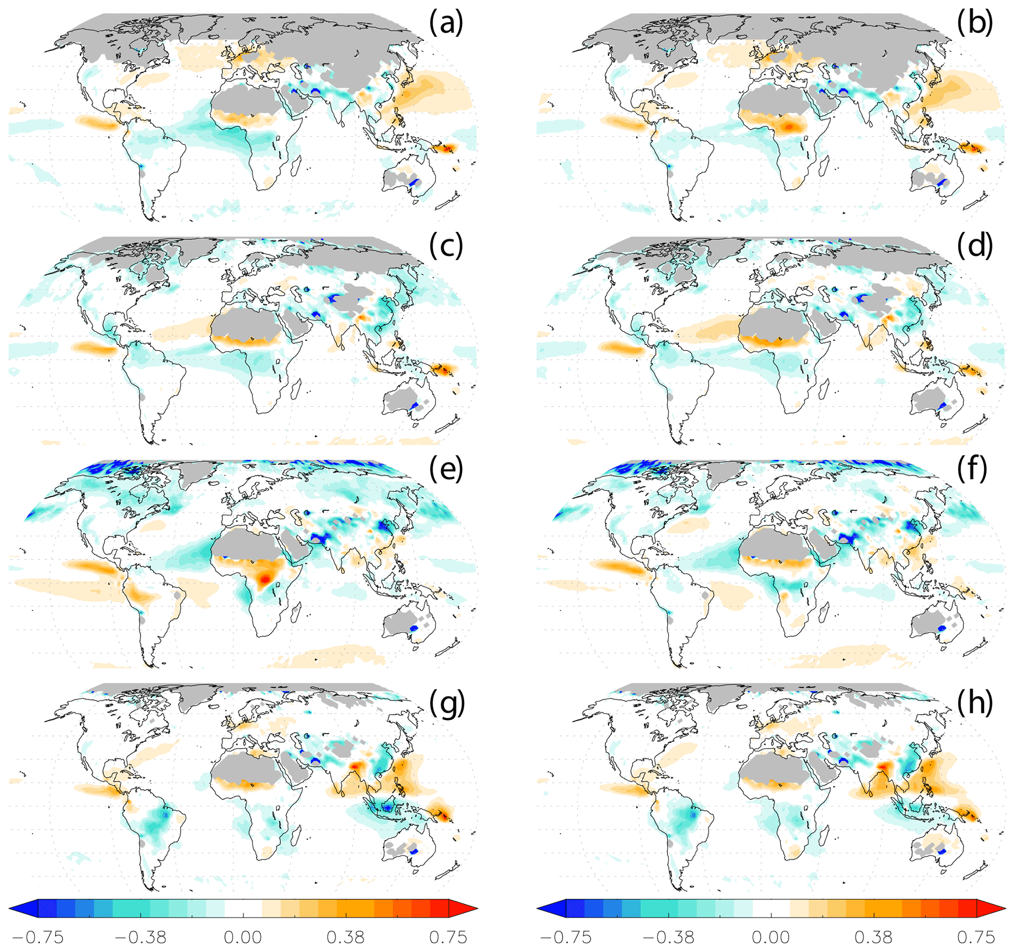
Figure 11 The difference in monthly modeled clear-sky aerosol optical depth (AOD) and MODIS Aqua (model – satellite). Model simulations using pyrE fire emissions (left) and model simulations using offline GFED4s emissions (right) are shown: January (a, b), April (c, d), July (e, f), and October (g, h). The difference is based on an ensemble of 10 simulations and 2003–2007 MODIS climatological monthly data. Missing MODIS data are shaded in light gray.

Finally, we demonstrate the contribution of BB emissions to total clear-sky AOD by comparing the simulations with both prescribed and interactive fire emissions to a simulation that has no fire emissions at all (Fig. 12). In the simulation with prescribed fire emissions, clear-sky AOD is on average 10 % higher than it is in a simulation with no fire emissions. In a simulation with pyrE, clear-sky AOD is about 7.5 % higher than it is in a simulation with no fire emissions. The impact of BB emissions on AOD is most pronounced in the source regions of Africa and the Amazon. In those regions the difference in AOD varies between 0.15 and 0.3. It is important to note that the differences in AOD are not only due to impact of BB emissions but also reflect climate variability, which impacts aerosol lifetime and interactive dust emissions.

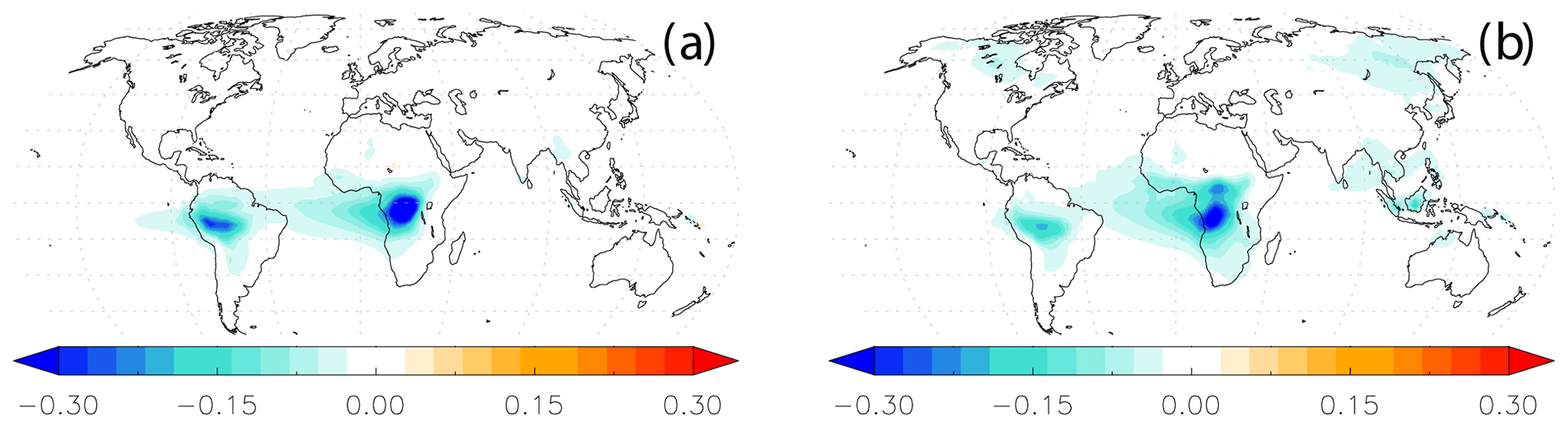
Figure 12 The difference in annual modeled clear-sky aerosol optical depth (AOD) between a simulation with no fire emissions to a simulation using pyrE fire emissions (a) and a simulation with offline GFED4s emissions (b). The difference (model with no fire emissions – model with fire emissions) is based on an ensemble of 10 simulations.

6 Conclusions

The development of pyrE allowed us for the first time to interactively simulate climate and fire activity with GISS ModelE2.1. The pyrE module, which is based on a the fire parameterizations of Pechony and Shindell (2009), was expanded to include fire spread and burned area, following the approach by Li et al. (2012). This study set out to simulate the climatology of fires, and not individual fire events. Like only a few other fire models (Zou et al., 2019), pyrE was developed with consideration of regional behavior. The new fire suppression scheme depends on population density but also on geographic regions. The new scheme reflects more intense fire suppression in the USA and Middle East and revokes fire suppression in Africa, which improved the fire activity seasonality simulated by pyrE compared to satellite retrievals. Active fire seasonality is well simulated in the fire source regions: the Amazon, SH Africa, and NH Africa, with the exception of being biased low compared to MODIS during November–December. This is due to the lack in parameterization of intentional ignitions and agricultural fires.

The regional model skill of fire activity was also demonstrated in the simulated burned area. Burned area in Southern Hemisphere Africa was well simulated by the model, while less active fire regions like temperate and boreal North America, Boreal Asia, Europe, and Middle East were biased high compared to GFED4s. Other regions like Australia, northern sub-Saharan Africa in November–December, Central Asia and Southeast Asia in January–March were biased low. Though the seasonality of simulated burned area reflects that of simulated active fires, the bias of burned area compared to GFED4s data is at least double that of active fires. Burned area is a quantity that most fire models struggle with. Wind speed, a driver of burned area, is averaged over a coarse grid cell, with no feedback from fire heat and energy, which can be a contributing factor to the lower simulated burned area values. The prescribed rudimentary PFTs of the model are a simplified version of the real world and thus can be a source of additional uncertainty. Finally, the rate of spread of burned area, a function of the burning vegetation type, that pyrE and other fire models use is on the lower end of field observations. A higher rate of spread could help to both override the scaling factor used for burned area and to reduce the negative bias compared to GFED4s.

Unlike other fire models, fire emissions in pyrE are driven directly by fires instead of burned area. Emissions are based on online active fire calculations and offline emission factors derived as described in Sect. 2.6. In contrast to the fact that simulated active fires are biased high compared to MODIS, globally, fire emissions are biased low compared to GFED4s. Fire emissions are well simulated over the Southern Hemisphere with the exception of Australia. Emissions are biased low over the Northern Hemisphere including northern sub-Sahara, with the exception of NH South America, which is biased high. The bias of active fires compared to MODIS in Australia and in northern sub-Saharan Africa during November–December propagates to emissions. The emission factors, which were calculated offline using MODIS fire count and GFED4s fire emissions and were applied based on the prescribed PFTs of the model, have their own limitations. They are based on a training dataset of 7 years, which would introduce biases in regions where fire cycle is longer than 7 years. Also, they rely on the modeled PFTs, enhancing the emissions dependency on the prescribed PFT and the lack of peat. Emission factors do not distinguish between intentional and accidental fires; thus, they indirectly account for all fire emissions, which reduce existing biases, although the regional distribution of them will not match the locations of intentional fires, unless natural vegetation burning occurs in the vicinity.

Less emissions compared to GFED4s means lower column densities and lower AOD when comparing a simulation with interactive fires to one with prescribed fires. However, as these quantities depend on climate feedbacks including processes other than fire, e.g., additional emission sources, precipitation, deposition, transport, and chemistry, the differences between the two simulations dilute. Nonetheless, a comparison with MODIS AOD demonstrates that AOD from a simulation with interactive fire emissions is comparable to AOD from a simulation with prescribed fire emissions.

The work presented here highlights that timing matters just as much as magnitude. This is true for fire distribution, emissions, and atmospheric composition. Timing is also the reason why intentional ignition was excluded from pyrE. Intentional ignition, namely, land clearing and agricultural fires, depends on region- and crop-specific planting and harvesting times. To include it would require crop functionality in ModelE, which was not present during the time of our development. Further future development should focus on the inclusion of intentional ignition and agricultural fires which are seasonal in nature, derived from crop planting and land clearing times. This addition could perhaps improve model performance over regions like equatorial Asia, Southeast Asia, and Central America as well as override the global scaling factors applied to active fires and burned area. The use of scaling factors is a common practice among fire models and should be carefully and transparently documented. Also, enhancing the prescribed PFTs, especially via the addition of peat, is imperative when studying fires. Peat exists as well outside of tropical Asia. There are immense reservoirs of peat in Africa (Dargie et al., 2017), as well as the boreal regions (Yu, 2012), where it used to be trapped under permafrost. Peat will likely become an even bigger source of fire emissions in the future. Improvement of the cloud-to-ground lightning parameterization may also prove useful, as changes to natural ignition will likely have significant impacts on Australian and boreal fire emissions. Finally, given that the heat component of fires interacts with the climate system and can also be used to derive more accurate emissions, as demonstrated by Ichoku and Ellison (2014) and three of the 11 FireMIP models (Rabin et al., 2017), it is worthwhile taking it into consideration when developing new fire modeling capabilities.

Appendix A

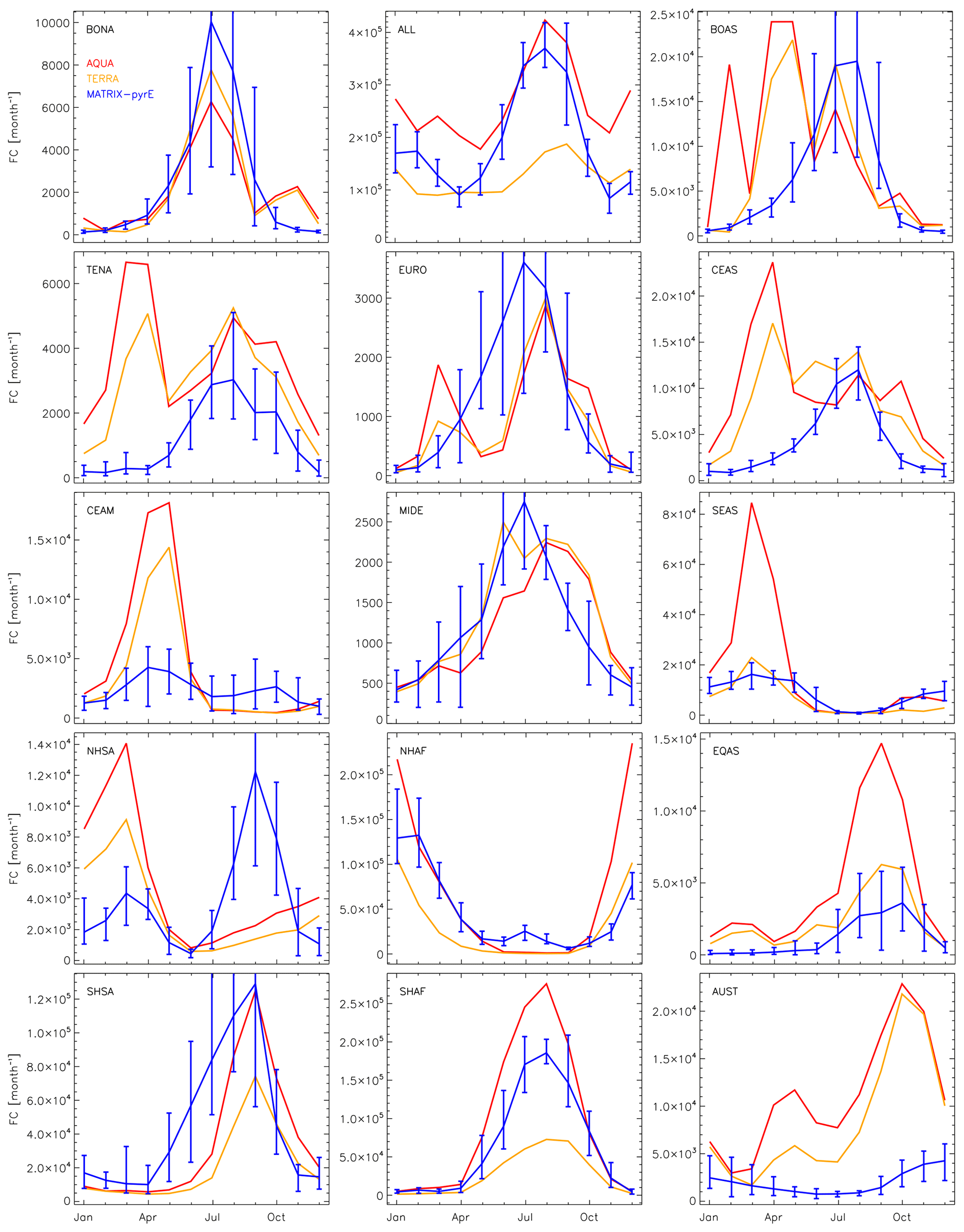
Figure A1 Seasonality of total active fires (FC) detected by MODIS Aqua (red) and Terra (orange) and simulated (blue) in all GFED regions (Fig. 1). Error bars represent the 10-year range in the simulations. Note the different scales in each panel.

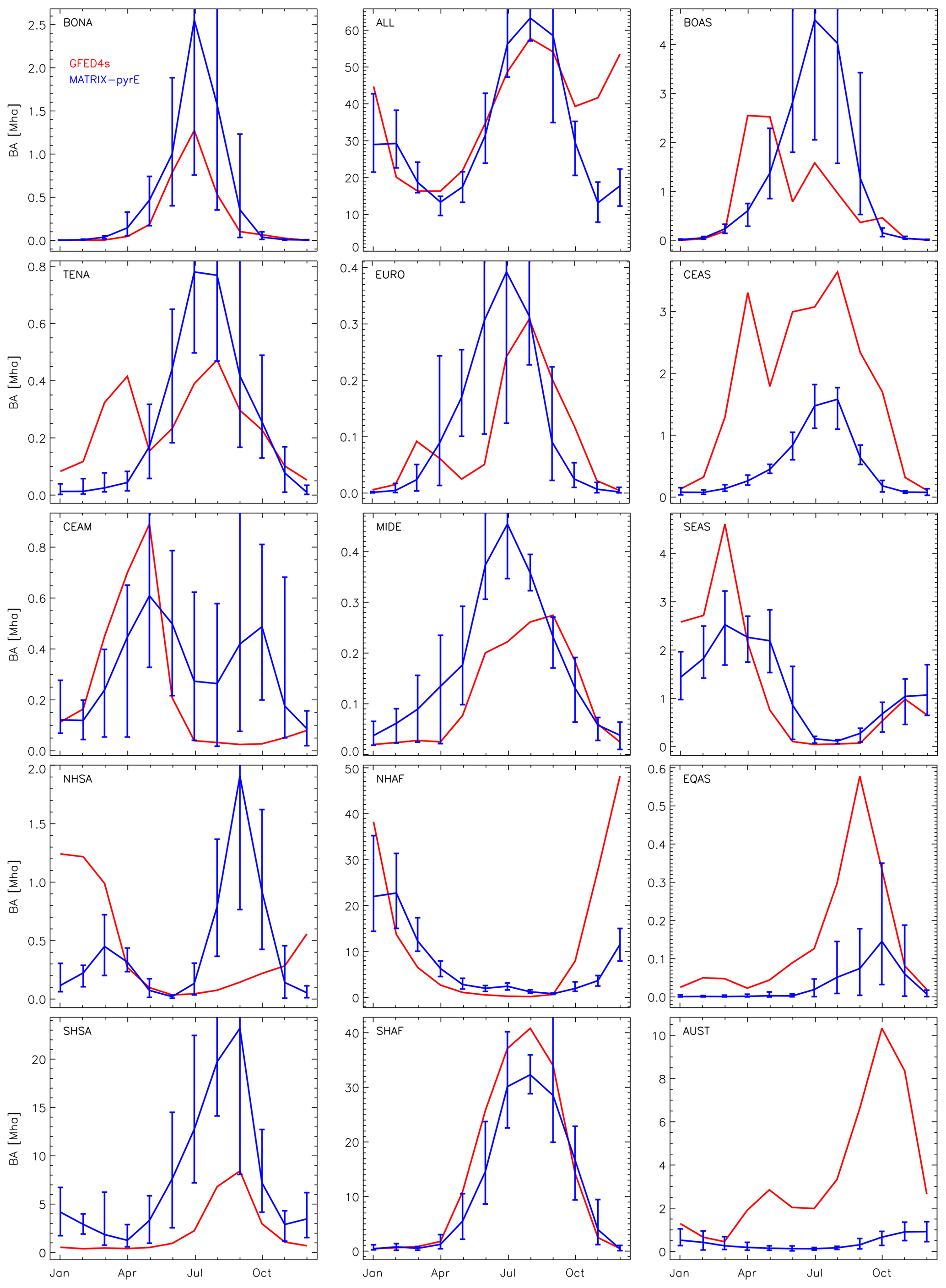
Figure A2 Seasonality of total burned area simulated (blue) and reported by GFED4s (red) in GFED regions. Error bars represent the 10-year range in the simulations. Note the different scales in each panel.

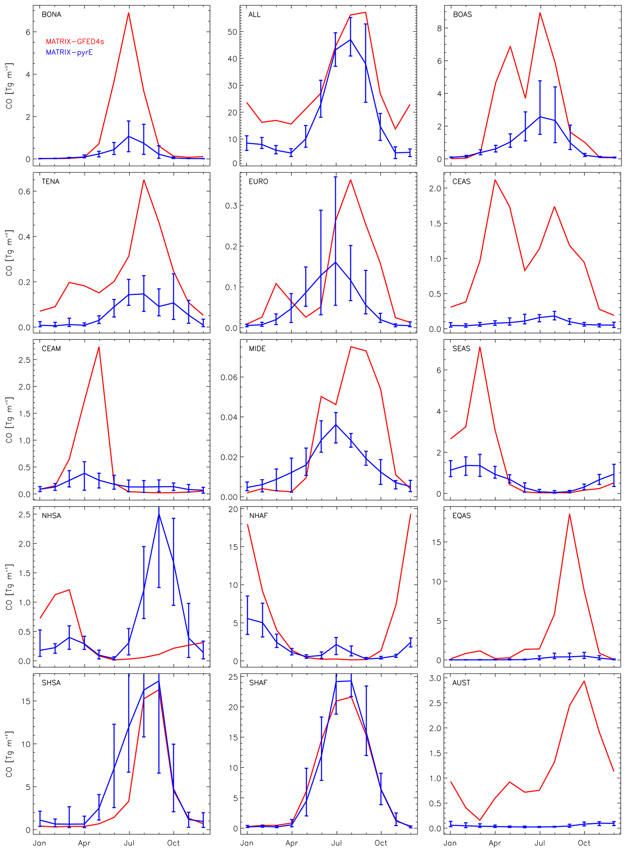
Figure A3 Seasonality of total fire CO emissions simulated (blue) and reported by GFED4s (red) in GFED regions. Error bars represent the 10-year range in the simulations. Note the different scales in each panel.

Figure A4 Seasonality of total fire organic aerosol (OA) emissions simulated (blue) and reported by GFED4s (red) in all GFED regions. Error bars represent the 10-year range in the simulations. Note the different scales in each panel.

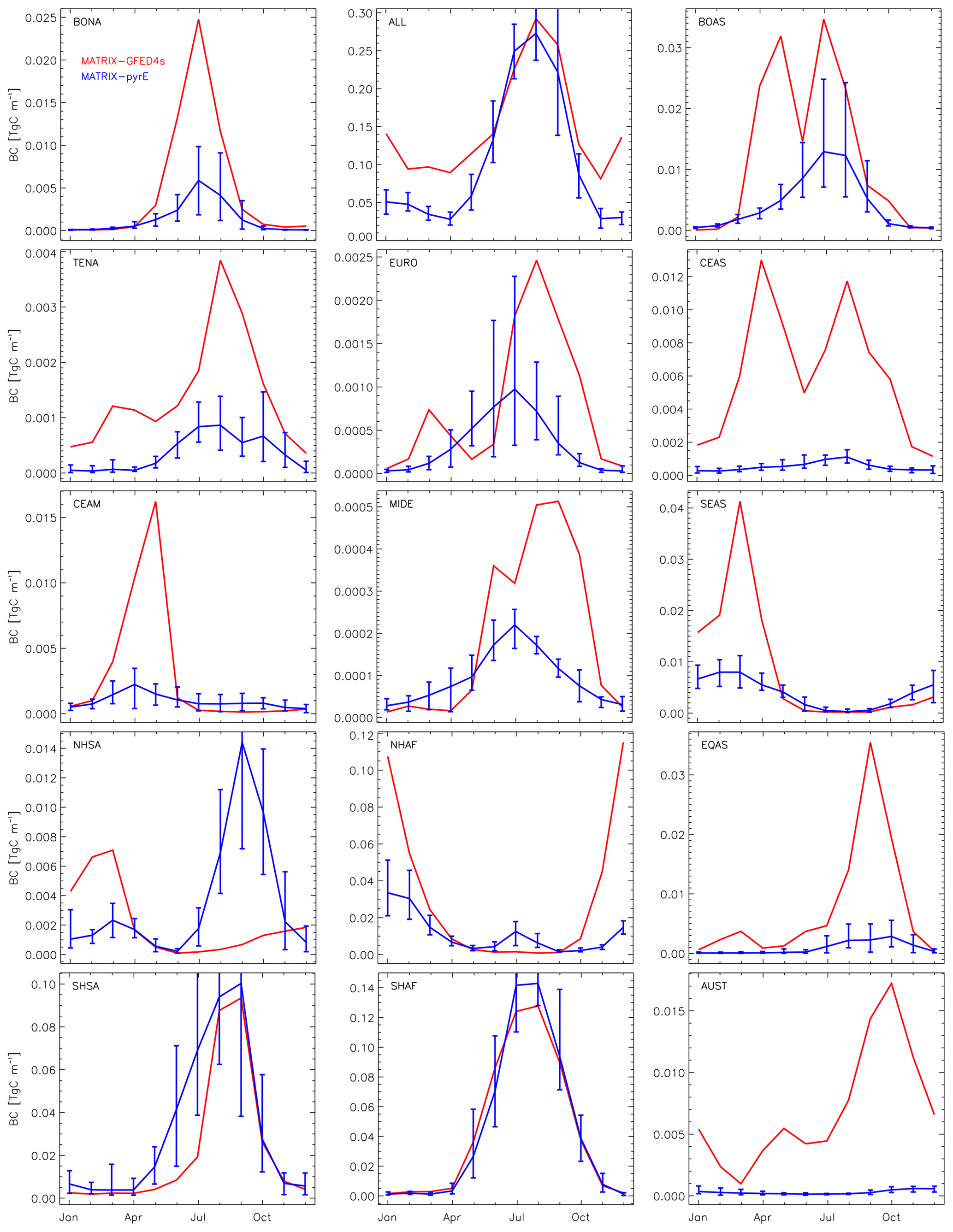
Figure A5 Seasonality of total fire BC emissions simulated (blue) and reported by GFED4s (red) in all GFED regions. Error bars represent the 10-year range in the simulations. Note the different scales in each panel.