the Creative Commons Attribution 4.0 License.
the Creative Commons Attribution 4.0 License.
Single-precision arithmetic in ECHAM radiation reduces runtime and energy consumption
Alessandro Cotronei
We converted the radiation part of the atmospheric model ECHAM to a single-precision arithmetic. We analyzed different conversion strategies and finally used a step-by-step change in all modules, subroutines and functions. We found out that a small code portion still requires higher-precision arithmetic. We generated code that can be easily changed from double to single precision and vice versa, basically using a simple switch in one module. We compared the output of the single-precision version in the coarse resolution with observational data and with the original double-precision code. The results of both versions are comparable. We extensively tested different parallelization options with respect to the possible runtime reduction, at both coarse and low resolution. The single-precision radiation itself was accelerated by about 40 %, whereas the runtime reduction for the whole ECHAM model using the converted radiation achieved 18 % in the best configuration. We further measured the energy consumption, which could also be reduced.
- Article
(19973 KB) - Full-text XML
- BibTeX
- EndNote
The atmospheric model ECHAM was developed at the Max Planck Institute for Meteorology (MPI-M) in Hamburg. Its development started in 1987 as a branch of a global weather forecast model of the European Centre for Medium-Range Weather Forecasts (ECMWF), thus leading to the acronym (EC for ECMWF, HAM for Hamburg). The model is used in different Earth system models (ESMs) as an atmospheric component, e.g., in the MPI-ESM also developed at the MPI-M; see Fig. 1. The current version is ECHAM 6 (Stevens et al., 2013). For a detailed list on ECHAM publications we refer to the home page of the institute (https://mpimet.mpg.de, last access: 22 April 2020). Version 5 of the model was used in the 4th Assessment Report of the Intergovernmental Panel on Climate Change (IPCC, 2007) and version 6 in the Coupled Model Intercomparison Project CMIP (World Climate Research Programme, 2019a).
The motivation for our work was the use of ECHAM for long-time paleo-climate simulations in the German national climate modeling initiative “PalMod: From the Last Interglacial to the Anthropocene – Modeling a Complete Glacial Cycle” (https://www.palmod.de, last access: 22 April 2020). The aim of this initiative is to perform simulations for a complete glacial cycle, i.e., about 120 000 years, with fully coupled ESMs.
The feasibility of long-time simulation runs highly depends on the computational performance of the models used. As a consequence, one main focus in the PalMod project is to decrease the runtime of the model components and the coupled ESMs.
In ESMs that use ECHAM, the part of the computational time that is used by the latter is significant. It can be close to 75 % in some configurations. Within ECHAM itself, the radiation takes the most important part of the computational time. As a consequence, the radiation part is not called in every time step in the current ECHAM setting. Still, its part of the overall ECHAM runtime is relevant; see Fig. 2.
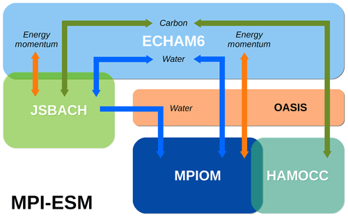
Figure 1Schematic of the structure of the Earth system model MPI-ESM with atmospheric component ECHAM, terrestrial vegetation model JSBACH, ocean model MPI-OM, marine biogeochemical model HAMOCC and OASIS coupler.
In the PalMod project, two different strategies to improve the performance of the radiation part are investigated: one is to run the radiation in parallel on different processors; the other one is the conversion to single-precision arithmetic we present in this paper. For both purposes, the radiation code was isolated from the rest of the ECHAM model. This technical procedure is not described here.
The motivation for the idea to improve the computational performance of ECHAM by a conversion to reduced arithmetic precision was the work of Vana et al. (2017). In this paper, the authors report on the conversion of the Integrated Forecasting System (IFS) model to single precision, observing a runtime reduction of 40 % in short-time runs of 12 or 13 months and a good match of the output with observational data. Here, the terms single and double precision refer to the IEEE-754 standard for floating-point numbers (IEEE Standards Association, 2019), therein also named binary64 and binary32, respectively. In the IEEE standard, an even more reduced precision, the half precision (binary16) format, is also defined. The IFS model, also developed by the ECMWF, is comparable to ECHAM in some respects since it also uses a combination of spectral and grid-point-based discretization. A similar runtime reduction of 40 % was reported by Rüdisühli et al. (2014) with the COSMO model that is used by the German and Swiss weather forecast services. The authors also validated the model output by comparing it to observations and the original model version.
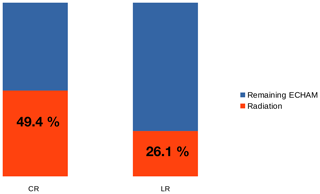
Figure 2Time consumption of the radiation part with regard to the whole ECHAM model in coarse (CR) and low resolution (LR) of standard PalMod experiments. The difference occurs since in these configurations the radiation part is called every 2 h, i.e., only every fourth (in CR) or every eighth time step (LR).
Recently, the use of reduced-precision arithmetic has gained interest for a variety of reasons. Besides the effect on the runtime, a reduction of energy consumption is also mentioned; see, e.g., Fagan et al. (2016), who reported a reduction by about 60 %. In the growing field of machine learning, single or even more reduced precision is used to save both computational effort as well as memory, motivated by the use of graphical processing units (GPUs). Dawson and Düben (2017) used reduced precision to evaluate model output uncertainty. For this purpose, the authors developed a software where a variable precision is available, but a positive effect on the model runtime was not their concern.
The process of porting a simulation code to a different precision highly depends on the design of the code and the way in which basic principles of software engineering have been followed during the implementation process. These are modularity, the use of clear subroutine interfaces, the way of data are transferred via a parameter list or global variables, etc. The main problem in legacy codes with a long history (as ECHAM) is that these principles were not usually applied very strictly. This is a general problem in computational science software, not only in climate modeling; see, for example, Johanson and Hasselbring (2018).
Besides the desired runtime reduction, a main criterion to assess the result of the conversion to reduced precision is the validation of the results, i.e., their differences to observational data and the output of the original, double-precision version. We carried out experiments on short timescales of 30 years with a 10-year spin-up. It has to be taken into account that after the conversion, a model tuning process (in the fully coupled version) might be necessary. This will require a significant amount of work to obtain an ESM that produces a reasonable climate; see, e.g., Mauritsen et al. (2012) for a description of the tuning of the MPI-ESM.
The structure of the paper is as follows: in the following section, we describe the situation from where our study and conversion started. In Sect. 3, we give an overview of possible strategies to perform a conversion to single-precision and discuss their applicability and finally the motivation for the direction we took. In Sect. 4, we describe changes that were necessary at some parts of the code due to certain constructs or libraries used, and in Sect. 5 we describe the parts of the code that need to remain at higher precision. In Sect. 6, we present the obtained results with regard to runtime reduction, output validation and energy consumption. At the end of the paper, we summarize our work and draw some conclusions.
The current major version of ECHAM, version 6, is described in Stevens et al. (2013). ECHAM is a combination of a spectral and a grid-based finite difference model. It can be used in five resolutions, ranging from the coarse resolution (CR) or T31 (i.e., a truncation to 31 wave numbers in the spectral part, corresponding to a horizontal spatial resolution of 96×48 points in longitude and latitude) to XR or T255. We present results for the CR and LR (low resolution, T63, corresponding to 192×96 points) versions. Both use 47 vertical layers and (in our setting) time steps of 30 and 15 min, respectively.
ECHAM6 is written in free-format Fortran and conforms to the Fortran 95 standard (Metcalf et al., 2018). It consists of about 240 000 lines of code (including approximately 71 000 lines of the JSBACH vegetation model) and uses a number of external libraries including LAPACK, BLAS (for linear algebra), MPI (for parallelization) and NetCDF (for in- and output). The radiation part that we converted contains about 30 000 lines of code and uses external libraries as well.
The basic ECHAM version we used is derived from the stand-alone version ECHAM-6.03.04p1. In this basic version, the radiation was modularly separated from the rest of ECHAM. This offers the option of running the radiation and the remaining part of the model on different processors in order to reduce the running time by parallelization, but it also maintains the possibility of running the ECHAM components sequentially. It was shown that the sequential version reproduces bit-identical results to the original code.
All the results presented below are evaluated with the Intel Fortran compiler 18.0 (update 4) (Intel, 2017) on the supercomputer HLRE-3 Mistral, located at the German Climate Computing Center (DKRZ), Hamburg. All experiments used the so-called compute nodes of the machine.
In this section we give an overview of possible strategies for the conversion of a simulation code (as the radiation part of ECHAM) to single-precision arithmetic. We describe the problems that occurred while applying them to the ECHAM radiation part. At the end, we describe the strategy that finally turned out to be successful. The general target was a version that can be used in both single and double precision with as few changes to the source code as possible. Our goal was to achieve a general setting of the working precision for all floating-point variables at one location in one Fortran module. It has to be taken into account that some parts of the code might require double precision. This fact was already noticed in the report on conversion of the IFS model by Vana et al. (2017).
We will from now on refer to the single-precision version as sp and to the double-precision version as the dp version.
3.1 Use of a precision switch
One ideal and elegant way to switch easily between different precisions of the variables of a code in Fortran is to use a specification of the kind parameter for floating-point variables as shown in the following example.
For reasons of flexibility, the objective of our work was to have a radiation with such precision switch.
! define variable with prescribed working
 precision (wp):
real(kind = wp) :: x
The actual value of wp can then be easily switched in the following way:
! define different working precisions:
! single precision (4 byte):
integer, parameter :: sp = 4
! double precision (8 byte):
integer, parameter :: dp = 8
! set working precision:
integer, parameter :: wp = sp
The recommendation mentioned by Metcalf et al. (2018, Sect. 2.6.2) is to define the different values of the kind parameter by using the selected_real_kind function. It sets the precision actually used via the definition of the
desired number of significant decimals (i.e., mantissa length) and exponent range, depending on the options the machine and compiler offer. This reads as follows:
! define precision using significant
! decimals and exponent range:
integer :: sign_decimals = 6
integer :: exp_range = 37
integer, parameter :: sp =
 selected_real_kind(sign_decimals,
  exp_range)
...
integer, parameter :: dp =
 selected_real_kind(...,...)
! set working precision:
integer, parameter :: wp = sp
In fact, similar settings can be found in the ECHAM module rk_mo_kind,
but unfortunately they are not consistently used. Instead, kind = dp is used directly in several modules.
A simple workaround, namely assigning the value 4 to dp and declaring an additional precision for actual dp where needed, circumvents this problem.
Then, compilation was possible after some modifications (concerning MPI and NetCDF libraries and the module mo_echam_radkernel_cross_messages). The compiled code crashed at runtime because of internal bugs triggered by code in the module rk_mo_srtm_solver and other parts. These issues were solved later when investigating each code part with the incremental conversion method.
The cause of these bugs could not be easily tracked.
3.2 Source code conversion of most time-consuming subroutines
As mentioned above, the conversion of the whole ECHAM model code using a simple switch was not successful. Thus, we started to identify the most time-consuming subroutines and functions and converted them by hand. This required the conversion of input and output variables in the beginning and at the end of the respective subroutines and functions. The changes in the code are schematically depicted in Fig. 3.

Figure 3Necessary code changes to convert a subroutine/function from the original double-precision version (left) to single precision (right) with internal casting; modifications in red.
This procedure allowed an effective implementation of sp computations of the converted subroutines/functions. We obtained high runtime reduction in some code parts. But the casting overhead destroyed the overall performance, especially if there were many variables to be converted.
For example, a time-consuming part of the subroutine gas_optics_lw in the module mo_lrtm_gas_optics was converted in the above way.
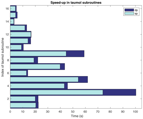
The converted part contains calls to subroutines taumol01 to taumol16, which were converted to sp. Figure 4 shows the runtime reduction for these subroutines, which was up to 30 %.
But the casting needed in the calling subroutine gas_optics_lw doubled the overall runtime in sp compared to dp.
The results of this evaluation lead to the following conclusion, which is not very surprising: the bigger the converted code block is with respect to the number of input and output variables, the lower the overhead for the casting will be in comparison to the gain in the calculations that are actually performed in sp. This was the reason for the decision to convert the whole radiation part of ECHAM, as it contains a relatively small amount of input/output variables.
3.3 Incremental conversion of the radiation part
As a result of the inefficient conversion of the most time-consuming subroutines or functions only, we performed a gradual conversion of the whole radiation code. For this purpose, we started from the lowest level of its calling tree, treating each subroutine/function separately. Consider an original subroutine on a lower level,
subroutine low(x_dp)
real(dp) :: x_dp
using dp variables.
We renamed it low_dp and made a copy in sp:
subroutine low_sp(x_sp)
real(sp) :: x_sp
We changed the dp version such that it just calls its sp counterpart, using implicit type conversions before and after the call:
subroutine low_dp(x_dp)
real(dp) :: x_dp
real(sp) :: x_sp
x_sp = x_dp
call low_sp(x_sp)
x_dp = x_sp
Now we repeated the same procedure with each subroutine/function that calls the original low, e.g.,
subroutine high(...)
call low(x_dp)
We again renamed it high_dp, generated an sp copy high_sp and defined an interface block (Metcalf et al., 2018):
interface low
   module procedure low_sp
   module procedure low_dp
end interface
In both high_dp and high_sp, we could now call the respective version of the lower-level subroutine passing either sp or dp parameters.
The use of the interface simplified this procedure significantly.
We then tested whether the model with the sp version of the subroutine/function compiles, whether it produces no runtime errors, and whether its difference to the dp version was in an “acceptable” range. Of course, the latter is a soft criterion, since a bit-identical result cannot be expected. Our criteria are explained below in Sect. 6.1. If the sp output was not acceptable in this sense, we marked the corresponding code part as requiring separate treatment, as described below in Sects. 4 and 5.
This procedure was repeated up to the highest level of the calling tree. It required a lot of manual work, but it allowed the examination of each modified part of the code, as well as a validation of the output data of the whole model.
In the ideal case and if no additional code changes had been necessary for the sp version, this would have led to consistent sp and dp versions. Finally, one of them could be renamed low, using wp for a working precision that could be set to sp or dp in some central module. Then, the interface also becomes redundant. This would be a model version that has a precision switch. The next section summarizes the few parts of the code that needed extra treatment.
Changing the floating-point precision in the radiation code required some modifications that are described in this section. Some of them are related to the use of external libraries, some others to an explicitly used precision-dependent implementation.
4.1 Procedure
In the incremental conversion, the precision variables dp and wp that are both used in the radiation code were replaced with sp.
Then in the final version, sp was replaced by wp.
With this modification, wp became a switch for the radiation precision.
As the original radiation contained several variables lacking explicit declaration of their precision, the respective format specifiers were added throughout.
4.2 Changes needed for the use of the NetCDF library
In the NetCDF library, the names of subroutines and functions have different suffixes depending on the precision used. They are used in the modules
rk_mo_netcdf, rk_mo_cloud_optics,
 rk_mo_lrtm_netcdf,
rk_mo_o3clim, rk_mo_read_netcdf77,
 rk_mo_srtm_netcdf.
In sp, they have to be replaced by their respective counterparts to read the NetCDF data with the correct precision. The script shown in Appendix A performs these changes automatically. This solution was necessary because an implementation using an interface was causing crashes for unknown reasons. It is possible that further investigation could lead to a working interface implementation for these subroutines/functions also at this point of the code.
4.3 Changes needed for parallelization with MPI
Several interfaces of the module mo_mpi were adapted to support sp. In particular
p_send_real,
p_recv_real
and p_bcast_real
were overloaded with sp subroutines for the array sizes needed. These modifications did not affect the calls to these interfaces.
No conversions are made in this module, so no overhead is generated.
4.4 Changes needed due to data transfer to the remaining ECHAM
In ECHAM, data communication between the radiation part and the remaining atmosphere is implemented in the module
mo_echam_radkernel_cross_messages
through subroutines using both MPI and the coupling library YAXT (DKRZ, 2013). Since it was not possible to have a mixed-precision data transfer for both libraries, our solution was to double the affected subroutines to copy and send both sp and dp data.
An additional variable conversion before or after their calls preserves the precision needed.
Also, in this case, interface blocks were used to operate with the correct precision.
The changed subroutines have the following prefixes: copy_echam_2_kernel, copy_kernel_2_echam, send_atm2rad and send_rad2atm. These modifications only affect the ECHAM model when used in the parallel scheme. They have a negligible overhead.
In the sp implementation of the radiation code, some parts still require higher precision to run correctly. These parts and the reasons for this are presented in this section. We want to emphasize that it is desirable to determine these reasons in more detail and to find alternatives in single-precision arithmetic that still give reasonable model output. However, this was beyond the scope of the project in which our work was conducted.
5.1 Overflow avoidance
When passing from dp to sp variables, the maximum representable number decreases from ≈10308 to ≈1038. In order to avoid an overflow that could lead to crashes, it is necessary to adapt the code to new thresholds. A similar problem could potentially occur for numbers which are too small (smaller than ).
As stated in the comments in the original code of psrad_interface, the following exponential needs conversion if not used in dp:
!this is ONLY o.k. as long as wp equals dp,
 else conversion needed
cisccp_cldemi3d(jl,jk,krow) = 1._wp -
 exp(-1._wp*cld_tau_lw_vr(jl,jkb,6))
One plausible reason for this is that the exponential is too big for the range of sp. Even though this line was not executed in the configuration used, we converted the involved quantities to dp. Since the variable on the left-hand side of the assignment was transferred within few steps to code parts outside the radiation, no other code inside the radiation had to be converted into dp.
Also module rk_mo_srtm_solver contained several parts sensitive to the precision.
First of all, the following lines containing the hard coded constant 500 could cause overflow as well:
exp_minus_tau_over_mu0(:) =
 inv_expon(MIN(tau_over_mu, 500._wp), kproma)
exp_ktau              (:) =
     expon(MIN(k_tau,       500._wp), kproma)
Here, expon and inv_expon calculate the exponential and inverse exponential of a vector (of length kproma in this case). The (inverse) exponential of a number close to 500 is too big (small) to be represented in sp.
In the configurations used, this line was not executed either. Nevertheless, we replaced this value by a constant depending on the precision used; see the script in Appendix A.
5.2 Numerical stability
Subroutine srtm_reftra_ec of module rk_mo_srtm_solver, described in Meador and Weaver (1979), was shown to be very sensitive to the precision conversion.
In this subroutine, a conversion to sp of just one of most internal variables separately was already causing crashes.
We introduced wrapper code for this subroutine to maintain the dp version.
The time necessary for this overhead was in the range of 3.5 % to 6 % for the complete radiation and between 0.6 % and 3 % for the complete ECHAM model.
In subroutine Set_JulianDay of the module rk_mo_time_base, the use of sp for the variable zd, defined by
zd = FLOOR(365.25_dp*iy)+INT(30.6001_dp*
 (im+1))  &
     + REAL(ib,dp)+1720996.5_dp+REAL(kd,dp)
     +zsec
caused crashes at the beginning of some simulation years.
In this case, the relative difference between the sp and the dp representation of the variable zd is close to machine precision (in sp arithmetic); i.e., the relative difference attains its maximum value. This indicates that code parts that use this variable afterwards are very sensitive to small changes in input data.
The code block was kept in dp by reusing existing typecasts, without adding new ones.
Thus, this did not increase the runtime. Rewriting the code inside the subroutine might improve the stability and avoid the typecasts completely.
5.3 Quadruple precision
The module rk_mo_time_base also contains some parts in quadruple (REAL(16)) precision in the subroutine
Set_JulianCalendar, e.g.,
zb = FLOOR(0.273790700698850764E-04_wp*
za-51.1226445443780502865715_wp)
Here wp was set to REAL(16) in the original code. This high precision was needed
to prevent roundoff errors because of the number of digits in the constants used.
We did not change the precision in this subroutine. But since we used wp as an indicator for the actual working precision, we replaced
wp by ap (advanced precision) to avoid conflicts with the working precision in this subroutine.
We did not need to implement any precision conversion, since all input and output variables are converted from and to integer numbers inside the subroutine anyway.
In this section, we present the results obtained with the sp version of the radiation part of ECHAM. We show three types of results, namely a comparison of the model output, the obtained gain in runtime and finally the gain in energy consumption.
The results presented below were obtained with the AMIP experiment (World Climate Research Programme, 2019b) by using the coarse (CR, T031L47) or low (LR, T063L47) resolutions of ECHAM. The model was configured with the cdi-pio parallel input–output option (Kleberg et al., 2017).
We used the following compiler flags (Intel, 2017), which are the default ones for ECHAM:
-
-O3: enables aggressive optimization, -
-fast-transcendentals,-no-prec-sqrt,-no-prec-div: enable faster but less precise transcendental functions, square roots and divisions, -
-fp-model source: rounds intermediate results to source-defined precision, -
-xHOST: generates instructions for the highest instruction set available on the compilation host processor, -
-diag-disable 15018: disables diagnostic messages, -
-assume realloc_lhs: uses different rules (instead of those of Fortran 2003) to interpret assignments.
6.1 Validation of model output
To estimate the output quality of the sp version, we compared its results with
-
the results of the original, i.e., the dp version of the model
-
and observational data available from several datasets.
We computed the difference between the outputs of the sp and dp versions and the differences of both versions to the observational data. We compared the values of
-
temperature (at the surface and at 2 m height), using the CRU TS4.03 dataset (University of East Anglia Climatic Research Unit et al., 2019),
-
precipitation (sum of large scale and convective precipitation in ECHAM), using the GPCP data provided by the NOAA/OAR/ESRL PSD, Boulder, Colorado, USA (Adler et al., 2003).
-
cloud radiative effect (CRE at the surface and at the top of the atmosphere, the latter split into longwave and shortwave parts), using the CERES EBAF datasets release 4.0 (Loeb and National Center for Atmospheric Research Staff, 2018).
In all results presented below, we use the monthly mean of these variables as basic data. This is motivated by the fact that we are interested in long-time simulation runs and climate prediction rather than in short-term scenarios (as for weather prediction). Monthly means are directly available as output from ECHAM.
All computations have been performed with the use of the Climate Data Operators (CDOs) (Schulzweida, 2019).
We emphasize that we present results for the output of the whole ECHAM model only. It would be also valuable to investigate the differences in the output of the two versions (dp and sp) of the radiation code alone, ideally when just using them for single atmospheric columns. This investigation was beyond the scope of our work here.
6.1.1 Difference in RMSE between single and double versions and observational data
We computed the spatial root mean square error (RMSE) of the monthly means for both sp and dp versions and the above variables. We applied the same metric for the difference between the outputs of the sp and dp versions. We computed these values over time intervals where observational data were available in the datasets used. For temperature and precipitation, these were the years 1981–2010 and for CRE the years 2000–2010 or 2001–2010. In all cases, we started the computation in the year 1970, having a reasonable time interval as spin-up.
Figure 5 shows the temporal behavior of the RMSE and the differences between sp and dp version, as they evolve in time. It can be seen that the RMSEs of the sp version are of the same magnitude as those of the dp version. Also, the differences between both versions are of similar or even smaller magnitude. Moreover, all RMSEs and differences do not grow in time. They oscillate but stay of the same order of magnitude for the whole considered time intervals.
Additionally, we averaged these values over the respective time intervals. Table 1 again shows that the RMSEs of the sp version are of the same magnitude as those of the dp version. Also, the differences between both versions are of similar or smaller magnitude.
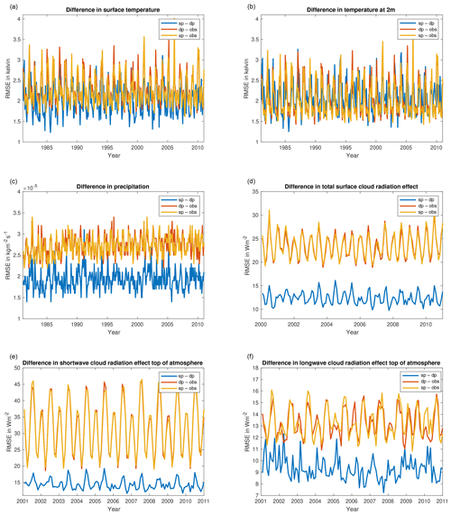
Figure 5Spatial RMSE of monthly means for sp and dp versions and differences between them in the same metric for (from top left to bottom right) temperature at the surface and at 2 m, precipitation, total CRE at the surface, and longwave and shortwave part of CRE at top of the atmosphere.
Table 1Spatial RMSE of monthly means for sp and dp versions and difference of both versions in the same metric, for selected model variables, averaged over the respective time spans (obs: observational data).

Moreover, we compared our obtained differences with the ones between two runs of the ECHAM versions 6.3.02 and 6.3.02p1. The differences between sp and dp version are of the same magnitude as the differences between these two model versions.
6.1.2 Spatial distribution of differences in the annual means
We also studied the spatial distribution of the differences in the annual means. Again we considered the differences between the sp and dp versions and the output of both versions and the observations. Here we included the signs of the differences and no absolute values or squares. For the given time spans, this results in a function of the form
for two variables or datasets y,z of monthly data. We performed this evaluation with #months in time span set to 12 for every year in the considered interval of 30 years. This procedure can be used to see if some spatial points or areas are constantly warmer or colder over longer time ranges. It is also a first test of the model output. However, it is clearly not sufficient for validation because errors may cancel out over time. The results are shown in Figs. 6 to 11.
Additionally, we performed a statistical analysis of the annual means of the sp version. We checked the hypothesis that the 30-year mean (in the interval 1981–2010) of the sp version equals the one of the original dp version. For this purpose, we applied a two-sided t test, using a consistent estimator for the variance of the annual means of the sp version. The corresponding values are shown in the second rows in Figs. 6 to 11. In this test, absolute values below 2.05 are not significant at the 95 % confidence level. For all considered variables, it can be seen that only very small spatial regions show higher values.
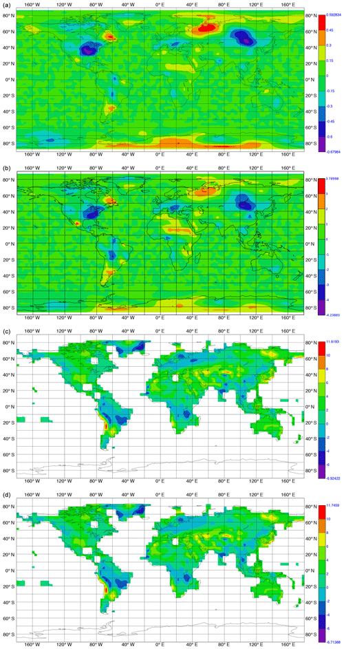
Figure 6Differences in temporal mean over the time interval 1981 to 2010 in temperature at the surface in kelvin. (a) Difference between sp and dp versions; (b) between the values of two-sided t test with respect to variance of the annual sp output – absolute values below 2.05 are not significant at the 95 % confidence level; (c) between dp version and observational data; (d) between sp version and observational data.
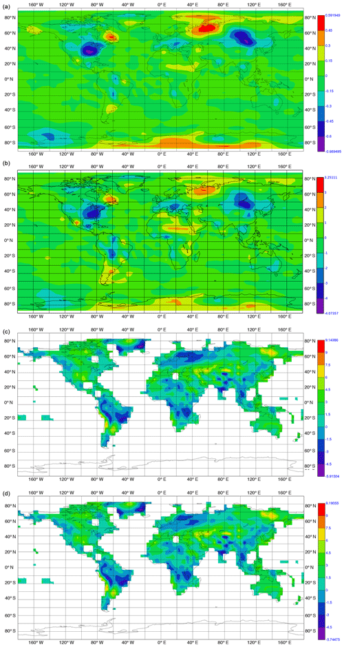
Figure 7As Fig. 6, but for temperature at 2 m.
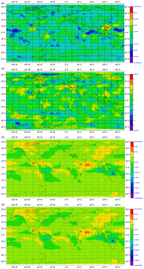
Figure 8As Fig. 6, but for precipitation in kilograms per square meter per second.
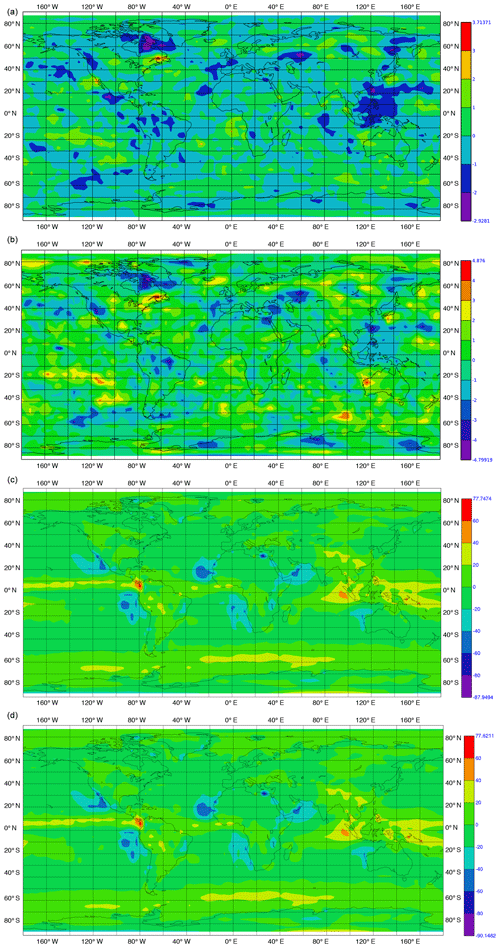
Figure 9As Fig. 6, but for surface cloud radiation effect in watts per square meter. Here, the differences to observations are for 2000–2010.
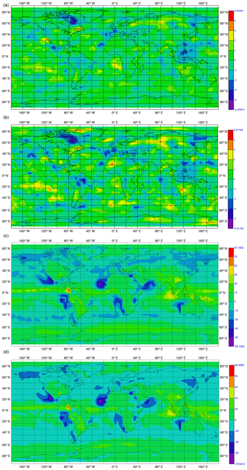
Figure 10As Fig. 9, but for longwave cloud radiation effect at the top of the atmosphere.
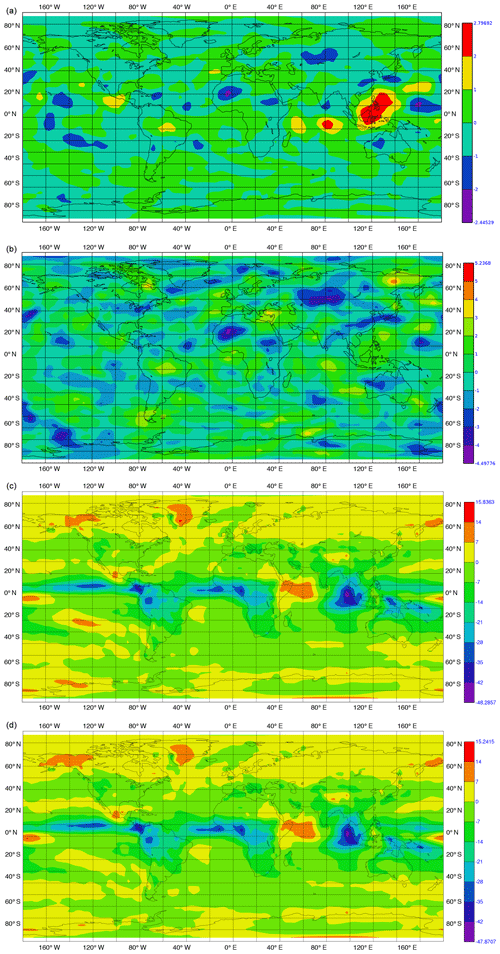
Figure 11As Fig. 10, but for shortwave cloud radiation effect at the top of the atmosphere.
6.2 Runtime reduction
In this section we present the results of the obtained runtime reduction when using the modified sp radiation code in ECHAM. All presented values are relative runtime reductions, computed by the formula
Since the model is usually run on parallel hardware, there are several configuration options that might affect its performance and also the runtime reduction when using the sp instead of the dp radiation code. We used the Mistral HPC system at DKRZ with 1 to 25 nodes, each of which has two Intel® Xeon® E5-2680v3 12C 2.5GHz (“Haswell”) with 12 cores, i.e., using from 24 up to 600 cores. The options we investigated are as follows:
-
the number of nodes used.
-
the choices cyclic:block and cyclic:cyclic (in this paper simply referred to as block and cyclic) offered by the SLURM batch system (SchedMD®, 2019) used on Mistral. It controls the distribution of processes across nodes and sockets inside a node. If not specified otherwise, we refer to the block setting, which is the default in ECHAM.
-
different values of the ECHAM parameter nproma, the maximum block length used for vectorization. For a detailed description; see Rast (2014, Sect. 3.8).
We were interested in the best possible runtime reduction when using the sp radiation in ECHAM. We studied the runtime reduction achieved both for the radiation itself and for the whole ECHAM model for a variety of different settings of the options mentioned, for both CR and (with reduced variety) LR resolutions. Our focus lies on the CR version, since it is the configuration that is used in the long-time paleo-runs intended in the PalMod project.
The results presented in this section have been generated with the Scalable Performance Measurement Infrastructure for Parallel Codes (Score-P, 2019) and the internal ECHAM timer.
All time measurements are based on 1-year runs. The unit we use to present the results is the number of simulated years per day runtime. It can be computed by the time measurements of the 1-year runs. For the results for the radiation part only, these are theoretical numbers, since the radiation is not run stand-alone for 1 year in ECHAM. We include them to give an impression what might be possible when more parts of ECHAM or even the whole model would be converted to sp. Moreover, we wanted to see if the runtime reduction of 40 % achieved with the IFS model in Vana et al. (2017) could be reached.
To figure out if there are significant deviations in the runtime, we also applied a statistic analysis for 100 1-year runs. They showed that there are only very small relative deviations from the mean; see Table 2.
At the end of this section, we give some details on which parts of the radiation code benefit the most from the conversion to reduced precision and which ones would not.
6.2.1 Dependency of runtime and runtime reduction on parameter settings
In order to find out the highest possible runtime reduction when using the sp radiation code, we first analyzed the dependency of the runtime on the parameter nproma. For the CR resolution, we tested for 1 to 25 core nproma values from 4 to 256 in steps of 4. It can be seen in the two top left panels in Fig. 12 that for 24 nodes there is no big dependency on nproma for the original dp version, when looking at radiation only. For the sp version, the dependency is slightly bigger, which results in a variety of the achieved runtime reduction between 25 % to 35 %.
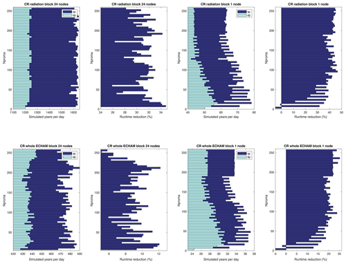
Figure 12Comparison of simulated model years per day cputime for sp and dp versions in coarse resolution (CR) for radiation part (top) and whole ECHAM (bottom) and for 1 and 24 nodes and values of nproma between 4 and 256, in steps of 4.
When looking at the results for the whole ECHAM model on the two left panels below in Fig. 12, it can be seen that the dependency of the runtime reduction on nproma becomes more significant.
Using only one node the performance for the dp version decreases with higher nproma, whereas the sp version does not show that big a dependency. The effect is stronger when looking at the radiation time only than for the whole ECHAM. For very small values of nproma, the sp version was even slower than the dp version. In particular, the default parameter value (nproma =12) for the sp version resulted in slower execution time than the corresponding dp version. An increased value of the parameter (nproma =48) made sp faster, even compared to the fastest nproma for dp (which was 24).
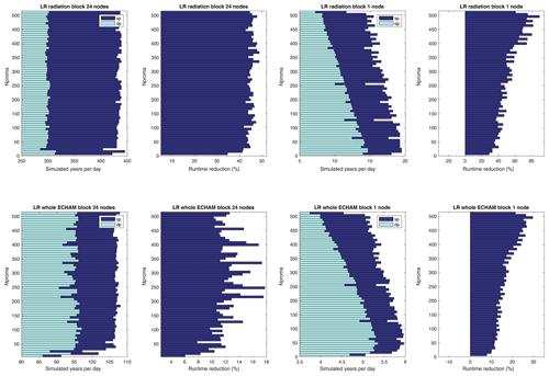
Figure 13As Figure 12, but for low resolution (LR) and values of nproma between 8 and 512, in steps of 8.
The difference between the block and cyclic options are not very significant for all experiments, even though cyclic was slightly faster in some cases. If not specified otherwise, we refer to the block setting (the default in ECHAM). The pictures for cyclic (not presented here) look quite similar.
Finally we note that measurements for shorter runs of only 1 month delivered different optimal values of nproma.
6.2.2 Best choice of parameter settings for CR configuration
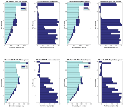
Motivated by the dependency on the parameter nproma observed above, we computed the runtime reduction when using the fastest choice. These runs were performed depending on the number of nodes used (from 1 to 25) in the CR configuration, for both block and cyclic options. The results are shown in Fig. 14. The corresponding best values of nproma are given in Tables 3 and 4.
It can be seen that for an optimal combination of number of nodes and nproma, the radiation could be accelerated by nearly 40 %. On the other hand, a bad choice of processors (here between 16 and 23) results in no runtime reduction or even an increase.
The runtime reduction for the whole ECHAM model with sp radiation was about 10 % to 17 %, when choosing an appropriate combination of nodes and nproma.
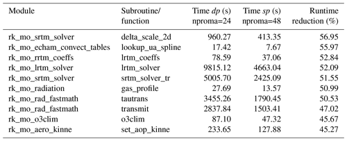
6.2.3 Parts of radiation code with biggest and smallest runtime reduction
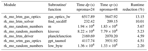
We identified some subroutines and functions with a very big and some with a very small runtime reduction by the conversion to sp. They are shown in Tables 5 and 6.
We could not achieve a significant runtime reduction in some cases because several time-consuming parts use expensive calculations with integer numbers, taking over 30 % of the total ECHAM time in some cases, e.g., in rk_mo_random_numbers. Therefore, these parts are not affected by the sp conversion.
6.3 Energy consumption
We also carried out energy consumption measurements. We used the IPMI (Intelligent Platform Management Interface) of the SLURM workload manager ADD (SchedMD®, 2019). It is enabled with the experiment option
#SBATCH --monitoring=power=5
Here we used one node with the corresponding fast configuration for nproma and the option cyclic. Simulations were repeated 10 times with a simulation interval of 1 year.
As Table 7 shows, the obtained energy reduction was 13 % and 17 % in blade and CPU power consumption, respectively. We consider these measurements only as a rough estimate. A deeper investigation of energy saving was not the focus of our work.
We have successfully converted the radiation part of ECHAM to single-precision arithmetic. All relevant parts of the code can now be switched from double to single precision by setting a Fortran kind parameter named wp either to dp or sp. There is one exception where a renaming of subroutines has to be performed. This can be easily done using a shell script (provided) before the compilation of the code.
We described our incremental conversion process in detail and compared it to other, in this case unsuccessful methods. Some small parts of the code had to remain at higher precision. Here, it would be desirable to further investigate how these parts may be replaced by alternative code or algorithms.
We tested the output for the single-precision version and found a good agreement with measurement data. The deviations over decadal runs are comparable to the ones of the double-precision versions. The difference between the two versions lie in the same range.
We achieved an improvement in runtime in coarse and low resolution of up to 40 % for the radiation itself and about 10 % to 17 % for the whole ECHAM. In this respect, we could support results obtained for the IFS model by Vana et al. (2017), where the whole model was converted. We also measured energy savings of about 13 % to 17 %. Moreover, we investigated the parts of the code that are sensitive to reduced precision and those parts which showed comparably high and low runtime reduction.
The information we provide may guide other people to convert even more parts of ECHAM to single precision. Moreover, they may also motivate them to consider a reduced-precision arithmetic in other simulation codes.
As a next step, the converted model part will be used in coupled ESM simulation runs over longer time horizons.
The following shell script converts the source code of ECHAM from double to single precision.
It renames subroutines and functions from the NetCDF library,
changes a constant in the code to avoid overflow (in a part that was not executed in the setting used), and
sets the constant wp that is used as Fortran kind attribute to the current working precision, either dp or sp.
A script that reverts the changes is analogous.
After the use of one of the two scripts, the model has to be re-compiled.
These scripts cannot be used on the standard ECHAM version but on the one mentioned in the code availability section.
#!/bin/bash
# script rad_dp_to_sp.sh
# To be executed from the root folder of ECHAM before compilation
for i in ./src/rad_src/rk_mo_netcdf.f90
         ./src/rad_src/rk_mo_srtm_netcdf.f90
         ./src/rad_src/rk_mo_read_netcdf77.f90
         ./src/rad_src/rk_mo_o3clim.f90
         ./src/rad_src/rk_mo_cloud_optics.f90;
do
   sed -i 's/_double/_real/g' $i
   sed -i 's/_DOUBLE/_REAL/g' $i
done
sed -i 's/numthresh = 500._wp/numthresh = 75._wp /g'
       ./src/rad_src/rk_mo_srtm_solver.f90
sed -i 's/INTEGER, PARAMETER :: wp = dp/INTEGER, PARAMETER :: wp = sp/g'
       ./src/rad_src/rk_mo_kind.f90
echo "ECHAM radiation code converted to single precision."
The code is available upon request. The conversion scripts (see Appendix A) and the output data for the single- and double-precision runs that were used to generate the output plots are available as NetCDF files under https://doi.org/10.5281/zenodo.3560536 (Slawig, 2019).
AC performed all experiments, generated a part of the plots and tables, and wrote parts of the paper. TS generated the other part of the plots and tables and wrote the main parts of the paper.
The authors declare that no competing interests are present.
The authors wish to thank Mohammad Reza Heidari, Hendryk Bockelmann and Jörg Behrens from the German Climate Computing Center DKRZ in Hamburg, Uwe Mikolajewicz and Sebastian Rast from the Max Planck Institute for Meteorology in Hamburg, Peter Düben from the ECMWF in Reading, Robert Pincus from Colorado University, Zhaoyang Song from the Helmholtz Centre for Ocean Research Kiel GEOMAR, and Gerrit Lohmann from AWI Bremerhaven and Bremen University for their valuable help and suggestions. Moreover, the authors would like to thank the anonymous reviewers for their corrections and helpful comments.
This research has been supported by the German Federal Ministry of Education and Research (BMBF) (grant no. FKZ: 01LP1515B).
This paper was edited by David Topping and reviewed by two anonymous referees.
Adler, R., Huffman, G., Chang, A., Ferraro, R., Xie, P., Janowiak, J., Rudolf, B., Schneider, U., Curtis, S., Bolvin, D., Gruber, A., Susskind, J., and Arkin, P.: The Version 2 Global Precipitation Climatology Project (GPCP) Monthly Precipitation Analysis (1979–Present), J. Hydrometeor., 4, 1147–1167, 2003. a
Dawson, A. and Düben, P. D.: rpe v5: an emulator for reduced floating-point precision in large numerical simulations, Geosci. Model Dev., 10, 2221–2230, https://doi.org/10.5194/gmd-10-2221-2017, 2017. a
DKRZ: Yet Another exChange Tool, available at: https://www.dkrz.de/redmine/projects/yaxt/wiki/Documentation (last access: 22 April 2020), 2013. a
Fagan, M., Schlachter, J., Yoshii, K., Leyffer, S., Palem, K., Snir, M., Wild, S., and Enz, C.: Overcoming the Power Wall by Exploiting Inexactness and Emerging COTS Architectural Features, Preprint ANL/MCS-P6040-0816, available at: http://www.mcs.anl.gov/publications (last access: 22 April 2020), 2016. a
IEEE Standards Association: IEEE Standard for Floating-Point Arithmetic, Tech. rep., avaialble at: https://ieeexplore.ieee.org/servlet/opac?punumber=8766227 (last access: 22 April 2020), 2019. a
Intel: Intel® Fortran Compiler 18.0 for Linux* Release Notes for Intel® Parallel Studio XE 2018, available at: https://software.intel.com/en-us/articles/intel-fortran-compiler-180-for-linux-release-notes-for-intel-parallel-studio-xe-2018 (last access: 22 April 2020), 2017. a, b
IPCC: Climate Change 2007: Synthesis Report, Contribution of Working Groups I, II and III to the Fourth Assessment Report of the Intergovernmental Panel on Climate Change, IPCC, Geneva, Switzerland, 2007. a
Johanson, A. and Hasselbring, W.: Software Engineering for Computational Science: Past, Present, Future, Comput. Sci. Eng., 20, 90–109, https://doi.org/10.1109/MCSE.2018.021651343, 2018. a
Kleberg, D., Schulzweida, U., Jahns, T., and Kornblueh, L.: CDI-pio, CDI with parallel I/O, available at: https://code.mpimet.mpg.de/attachments/download/13746/pio_docu.pdf (last access: 22 April 2020), 2017. a
Loeb, N. and National Center for Atmospheric Research Staff: The Climate Data Guide: CERES EBAF: Clouds and Earth's Radiant Energy Systems (CERES) Energy Balanced and Filled (EBAF), available at: https://climatedataguide.ucar.edu/climate-data/ceres-ebaf-clouds-and-earths-radiant-energy-systems-ceres-energy-balanced-and-filled (last access: 22 April 2020), 2018. a
Mauritsen, T., Stevens, B., Roeckner, E., Crueger, T., Esch, M., Giorgetta, M., Haak, H., Jungclaus, J., Klocke, D., Matei, D., Mikolajewicz, U., Notz, D., Pincus, R., Schmidt, H., and Tomassini, L.: Tuning the climate of a global model, J. Adv. Model. Earth Sy., 4, https://doi.org/10.1029/2012MS000154, 2012. a
Meador, W. E. and Weaver, W. R.: Two-Stream Approximations to Radiative Transfer in Planetary Atmosphere: A Unified Description of Existing Methods and a New improvement, J. Atmos. Sci., 37, 630–643, 1979. a
Metcalf, M., Reid, J., and Cohen, M.: Modern Fortran Explained, Numerical Mathematics and Scientific Computation, Oxford University Press, 2018. a, b, c
Rast, S.: Using and programming ECHAM6 – a first introduction, available at: https://www.mpimet.mpg.de/fileadmin/staff/rastsebastian/echam_6.1_lecture.pdf (last access: 22 April 2020), 2014. a
Rüdisühli, S., Walser, A., and Fuhrer, O.: COSMO in Single Precision, in: Cosmo Newsletter, 14, 70–87, Swiss Federal Office of Meteorology and Climatology MeteoSwiss, 2014. a
SchedMD®: Slurm workload manager, available at: https://slurm.schedmd.com (last access: 22 April 2020), 2019. a, b
Schulzweida, U.: Climate Data Operators User Guide, Max-Planck Institute for Meteorology, Hamburg, Germany, available at: https://code.mpimet.mpg.de/projects/cdo/embedded/cdo.pdf (last access: 22 April 2020), 1.9.8 edn., 2019. a
Score-P: Scalable Performance Measurement Infrastructure for Parallel Codes, available at: http://scorepci.pages.jsc.fz-juelich.de/scorep-pipelines/docs/scorep-4.1/html/index.html (last access: 22 April 2020), 2019. a
Stevens, B., Giorgetta, M., Esch, M., Mauritsen, T., Crueger, T., Rast, S., Salzmann, M., Schmidt, H., Bader, J., Block, K., Brokopf, R., Fast, I., Kinne, S., Kornblueh, L., Lohmann, U., Pincus, R., Reichler, T., and Roeckner, E.: Atmospheric component of the MPI-M Earth System Model: ECHAM6, J. Adv. Model. Earth Sy., 5, 146–172, https://doi.org/10.1002/jame.20015, 2013. a, b
Slawig, T.: Output of ECHAM with radiation code in single precision (Version 1.0) [Data set], Zenodo, https://doi.org/10.5281/zenodo.3560536, 2019. a
University of East Anglia Climatic Research Unit, Jones, P., and Harris, I.: Climatic Research Unit (CRU): Time-series (TS) datasets of variations in climate with variations in other phenomena v3, NCAS British Atmospheric Data Centre, 2019. a
Vana, F., Düben, P., Lang, S., Palmer, T., Leutbecher, M., Salmond, D., and Carver, G.: Single Precision in Weather Forecasting Models: An Evaluation with the IFS, Mon. Weather Rev., 145, 495–502, 2017. a, b, c, d
World Climate Research Programme: Coupled Model Intercomparison Project (CMIP), available at: https://www.wcrp-climate.org/wgcm-cmip (last access: 22 April 2020), 2019a. a
World Climate Research Programme: Atmospheric Model Intercomparison Project (AMIP), available at: https://www.wcrp-climate.org/modelling-wgcm-mip-catalogue/modelling-wgcm-mips-2/240-modelling-wgcm-catalogue-amip (last access: 22 April 2020), 2019b. a
- Abstract
- Introduction
- Configuration of ECHAM used
- Strategies for conversion to single precision
- Necessary changes in the radiation code
- Parts still requiring higher precision
- Results
- Conclusions
- Appendix A: Conversion script
- Code and data availability
- Author contributions
- Competing interests
- Acknowledgements
- Financial support
- Review statement
- References


