An intercomparison of tropospheric ozone reanalysis products from CAMS, CAMS interim, TCR-1, and TCR-2

Global tropospheric ozone reanalyses constructed using different state-of-the-art satellite data assimilation systems, prepared as part of the Copernicus Atmosphere Monitoring Service (CAMS-iRean and CAMS-Rean) as well as two fully independent reanalyses (TCR-1 and TCR-2, Tropospheric Chemistry Reanalysis), have been intercompared and evaluated for the past decade. The updated reanalyses (CAMS-Rean and TCR-2) generally show substantially improved agreements with independent ground and ozone-sonde observations over their predecessor versions (CAMS-iRean and TCR-1) for diurnal, synoptical, seasonal, and interannual variabilities. For instance, for the Northern Hemisphere (NH) mid-latitudes the tropospheric ozone columns (surface to 300 hPa) from the updated reanalyses show mean biases to within 0.8 DU (Dobson units, 3 % relative to the observed column) with respect to the ozone-sonde observations. The improved performance can likely be attributed to a mixture of various upgrades, such as revisions in the chemical data assimilation, including the assimilated measurements, and the forecast model performance. The updated chemical reanalyses agree well with each other for most cases, which highlights the usefulness of the current chemical reanalyses in a variety of studies. Meanwhile, significant temporal changes in the reanalysis quality in all the systems can be attributed to discontinuities in the observing systems. To improve the temporal consistency, a careful assessment of changes in the assimilation configuration, such as a detailed assessment of biases between various retrieval products, is needed. Our comparison suggests that improving the observational constraints, including the continued development of satellite observing systems, together with the optimization of model parameterizations such as deposition and chemical reactions, will lead to increasingly consistent long-term reanalyses in the future.

1 Introduction

Both human activity and natural processes influence the global distribution of present-day tropospheric ozone, together with its interannual variability and trends. Amongst other factors, increments in surface ozone concentrations contribute to changes in air quality (e.g. Im et al., 2018), human health (Liang et al., 2018), and agriculture (van Dingenen et al., 2009). Owing to its radiative effects, tropospheric ozone is an important driver in climate change (Checa-Garcia et al., 2018). Also, it may affect long-range weather forecasts, even if in evaluations no improvement has been detected so far (Cheung et al., 2014). Considering its lifetime of a few weeks, tropospheric ozone can be controlled by both local and remote pollution sources through atmospheric chemical processes and long-range transport (Monks et al., 2015; Huang et al., 2017; Jonson et al., 2018), as well as stratospheric influx (e.g. Hsu and Prather, 2009; Knowland et al., 2017). In addition to anthropogenic sources, natural processes such as El Niño–Southern Oscillation (ENSO) conditions affect tropospheric ozone production and loss terms through changes in upwelling, convection, solar irradiance, humidity, and biomass-burning emissions (e.g. Ziemke and Chandra, 2003, Inness et al., 2015). Other processes that potentially influence tropospheric ozone, which are generally considered of minor importance, are the Quasi-biennial Oscillation (Neu et al., 2014) and the North Atlantic Oscillation (Thouret et al., 2006).

Various types of datasets have been compiled to allow for the analysis of the current state of tropospheric ozone and its changes over time. Surface ozone is reasonably well monitored through in situ networks measuring surface concentrations (Global Atmosphere Watch (GAW), Global Monitoring Division (GMD), European Monitoring and Evaluation Programme (EMEP), AirNow), as collected and homogenized by the Tropospheric Ozone Assessment Report (TOAR; Schultz et al., 2017a, b). Above the ground, ozone is monitored through ozone-sondes, collected by the World Ozone and Ultraviolet Radiation Data Centre (WOUDC; https://woudc.org/, last access: 20 March 2020) and aircraft (In-service Aircraft for a Global Observing System (IAGOS); Nédélec et al., 2015). These observations are complemented with (combined) satellite observations from instruments such as Global Ozone Monitoring Experiment 2 (GOME-2), Ozone Monitoring Instrument (OMI), Microwave Limb Sounder (MLS), Infrared Atmospheric Sounding Interferometer (IASI), and Tropospheric Emission Spectrometer (TES). Here each retrieval product comes with its specific (vertical) sensitivity, which allows for the derivation of tropospheric ozone columns as listed in Gaudel et al. (2018).

The multitude of observational datasets have led to observationally constrained assessments of the current state and trends in tropospheric ozone, as for instance documented as part of TOAR (Schultz et al., 2017a; Gaudel et al., 2018; Fleming et al., 2018; Tarasick et al., 2019). Recent studies have also shown decadal-scale changes in global tropospheric ozone using various observations, such as a shift in the seasonal cycle at Northern Hemisphere (NH) mid-latitudes and long-term trends over many regions (e.g. Parrish et al., 2014; Cooper et al., 2014; Gaudel et al., 2018; Fleming et al., 2018). Based on a combination of multiple ozone retrieval products, Ziemke et al. (2019) have inferred positive trends in tropospheric ozone trends, particularly in the 2005–2016 time period.

Additional coordination with the emphasis on modelling activities related to tropospheric ozone has been established, for instance, to analyse the contribution of ozone to air quality (AQMEII: Air Quality Modelling Evaluation International Initiative), the impact of long-range transport on air quality (HTAP: Hemispheric Transport of Air Pollution), and the impact of composition changes on climate change (CCMI: Chemistry-Climate Model Initiative) (e.g. Young et al., 2013; Morgenstern et al., 2018; Liang et al., 2018).

Following the concept of meteorological reanalyses such as ERA5 (Hersbach et al., 2018), observationally constrained reanalyses of the atmospheric chemical composition have been developed to provide time series of tropospheric and stratospheric ozone. A reanalysis is a systematic approach to create long-term data assimilation products by combining a series of observational datasets with a model. Advanced data assimilation, such as four-dimensional variational data assimilation (4D-Var) and ensemble Kalman filter (EnKF), allows for the propagation of observational information in time and space and, from a limited number of observed species, to an analysis of a wide range of chemical components. This can be used in reanalyses to provide consistent global fields that are in agreement with individual observations (Lahoz and Schneider, 2014; Bocquet et al., 2015). A reanalysis hence provides an instantaneous global image of atmospheric composition, together with its change over time, and therefore it serves in principle to analyse the mean state of the atmosphere, together with its variability and trends.

Applications of chemical reanalyses include comprehensive spatio-temporal evaluation of independent models, such as those developed in the framework of the Atmospheric Chemistry and Climate Model Intercomparison Project (ACCMIP; Young et al., 2013) and CCMI (Morgenstern et al., 2018). This was shown to be useful as evaluations using individual measurements are subject to significant sampling biases (Miyazaki and Bowman, 2017). In their study the ACCMIP ensemble ozone simulations were evaluated using a chemical reanalysis, complementing the use of individual measurements for such a purpose. The chemical reanalyses can also be used as an input to meteorological reanalyses, e.g. for radiation calculations (Dragani et al., 2018), and they can provide boundary conditions to regional-scale models and to analyse particular pollution events such as those associated with heatwaves or large-scale forest fires (Ordóñez et al., 2010; Huijnen et al., 2012, 2016). Finally, they can be used as a reference to identify to what extent particular periods and regions deviate from climatology, as provided by the reanalysis, as for instance also discussed in the series of the “State of the Climate” (Flemming and Inness, 2018).

However, all of these applications presume that the reanalysis is sufficiently accurate or, at least, well described. Despite the range of observations assimilated into the respective systems, this is not necessarily ensured. Issues are multiple, and they depend on the availability of observations and on the modelling and data-assimilation framework with respect to the species and location under consideration. For tropospheric ozone reanalyses, state-of-the-art global analysis systems have been used to assimilate satellite-based observations, where satellite measurements have limited information on vertical profiles. In particular, the low measurement sensitivities to the lower troposphere make it difficult to correct near-surface ozone. Advanced satellite retrievals provide improved vertical resolution to the troposphere (Cuesta et al., 2018; Fu et al., 2018), but the temporal coverage and vertical resolution of these retrievals is still limited, and their application in data assimilation remains a challenge (Miyazaki et al., 2019a). This also implies that constraints on other parts of the system (other trace gases, aerosol, their emissions, and meteorology, driving the tracer transport and its removal) will strongly affect the quality of the reanalysis. Simultaneous optimization of concentrations and precursor emissions thus seems important in improving the analysis of lower tropospheric ozone (Miyazaki et al., 2012b). Furthermore, providing consistent time series over decadal timescales is challenging. The observational data from satellite instruments available for assimilation evolve over time with new instruments becoming available, while others cease to exist, and different satellite retrieval products typically show biases with respect to ground-based observations and with respect to each other.

In the framework of the Copernicus Atmosphere Monitoring Service (CAMS, https://atmosphere.copernicus.eu, last access: 20 March 2020), ECMWF's Integrated Forecasting System (IFS) has been extended to include modules for atmospheric chemistry, aerosols, and greenhouse gases. Using this system, three recent reanalyses have been released: the Monitoring Atmospheric Composition and Climate (MACC) reanalysis for the years 2003–2012 (Inness et al., 2015), the “CAMS interim Reanalysis” (hereafter CAMS-iRean) for the years 2003–2018 (Flemming et al., 2017), and recently the “CAMS Reanalysis” (CAMS-Rean) for the years 2003 to the present (Inness et al., 2019). Miyazaki et al. (2015) simultaneously estimated concentrations and emissions for the 8-year Tropospheric Chemistry Reanalysis (TCR-1) for the years 2005–2012 obtained from an assimilation of multi-constituent satellite measurements using an ensemble Kalman filter (EnKF). TCR-1 has been used to provide comprehensive information on atmospheric composition variability and elucidate variations in precursor emissions, as well as to evaluate bottom-up emission inventories (Miyazaki et al., 2012a, 2014, 2015, 2017; Ding et al., 2017; Jiang et al., 2018; Tang et al., 2019). A second version of the EnKF-based reanalysis (TCR-2) has been recently produced using an updated model and satellite retrievals for the years 2005–2018 (Kanaya et al., 2019; Miyazaki et al., 2019; Thompson et al., 2019). For stratospheric constituents, several studies have been conducted to produce and compare stratospheric chemical reanalysis products (Davis et al., 2017; Errera et al., 2019).

Here we evaluate the ability of the two CAMS and two TCR atmospheric composition reanalysis datasets to constrain tropospheric ozone variability. We do not evaluate the MACC reanalysis here, because it has been extensively documented in the past (Inness et al., 2013; Flemming et al., 2017; Bennouna et al., 2019) and only covered the 2003–2012 time period. Furthermore, it has been shown to suffer from significant spurious drifts in tropospheric ozone due to a bias-correction issue, which makes it less useful to assess its multiannual mean and interannual variability. In particular, Katragkou et al. (2015) discusses the ozone in the MACC reanalysis, while Inness et al. (2019) reports how CAMS-Rean compares to CAMS-iRean and MACC reanalyses.

To assess the quality of these reanalysis products, with attention to the various potential types of application described above, this study evaluates tropospheric ozone for a range of independent in situ observations: ozone-sondes from the World Ozone and Ultraviolet Radiation Data Centre (WOUDC), NOAA Earth System Research Laboratory (ESRL), and Southern Hemisphere Additional Ozonesondes (SHADOZ); monthly-mean gridded surface ozone as collected within TOAR; and individual surface ozone observations from the EMEP network.

In this study, we limit ourselves to tropospheric ozone in the reanalysis products, and we only refer, where relevant, to interactions with other components in the reanalysis systems, such as nitrogen oxides (NO_x), carbon monoxide (CO), and aerosols. Even though these four reanalysis products are not equally independent, each of their configurations shows substantial differences which are bound to impact the performance of the reanalysis products. This intercomparison aims to reveal to what extend the reanalysis products agree, depending on region and time periods. Temporal consistency is an important aspect when assessing long-term time series and intercomparing individual years. At the same time, this is a challenge because of the change in the observing system used to constrain the reanalysis products over the course of a decade or more, all having different retrieval specifications (see also Gaudel et al., 2018).

In the next sections we describe the various reanalysis products used in this paper (Sect. 2) and the observational data used for evaluation (Sect. 3). Evaluations against ozone-sondes are presented in Sect. 4 and against TOAR gridded surface ozone and EMEP surface observations in Sects. 5 and 6, respectively. We continue describing the reanalysis products through assessment of their global spatial and temporal consistency (Sect. 7). We end with discussions and conclusions in Sect. 8.

2 Chemical reanalysis products

The global atmospheric chemistry reanalysis products evaluated in this paper are listed in Table 1. The general configuration of the various data assimilation systems, together with details specific to tropospheric ozone analysis, is provided in the following subsections. For more detailed information on the specifications of the various reanalysis products, the reader is referred to the references.

Table 1 Overview of recent reanalysis products.

2.1 The CAMS interim Reanalysis

In CAMS, the data assimilation capabilities in IFS for trace gases and aerosols relies on the four-dimensional variational (4D-Var) technique, developed for the analysis of meteorological fields. The CAMS interim Reanalysis (CAMS-iRean; Flemming et al., 2017) has been the intermediate reanalysis between the widely used MACC Reanalysis (Inness et al., 2015) and the recently produced CAMS Reanalysis (Inness et al., 2019). The chemistry module as adopted in CAMS-iRean is described and evaluated in Flemming et al. (2015). It relies on the modified CB05 tropospheric chemistry mechanism as originating from TM5 (Huijnen et al., 2010; Williams et al., 2013), which contains 52 species and 130 (gas phase + photolytic) reactions; stratospheric ozone is modelled through the Cariolle parameterization (Cariolle and Teyssèdre, 2007). Anthropogenic emissions originate essentially from the MACCity inventory (Granier et al., 2011) with enhanced wintertime CO emissions over Europe and the US (Stein et al., 2014). Monthly specific biogenic emissions originate from MEGAN-MACC (Sindelarova et al., 2014) but using monthly climatological values from 2011 onwards. Daily biomass-burning emissions originate from GFASv1.2 (Kaiser et al., 2013). The meteorological model is IFS CY40R2.

In terms of ozone, observations from the following set of satellite instruments have been assimilated: Solar Backscatter ULTra-Violet (SBUV/2), OMI, MLS, GOME-2, SCanning Imaging Absorption spectroMeter for Atmospheric CHartographY (SCIAMACHY), GOME, and Michelson Interferometer for Passive Atmospheric Sounding (MIPAS); see also Table 2. A variational bias-correction (VarBC) scheme was applied to OMI, SCIAMACHY, and GOME-2 retrievals of total ozone columns to ensure optimal consistency of all information used in the analysis. SBUV/2 and also profile retrievals from MLS and MIPAS were assimilated without correction. Note that no total columns are assimilated for solar elevations less than 6^∘ (hence excluding polar winters).

Profile observations from limb instruments in the range of 0.1–150 hPa for MIPAS and 0.1–147 hPa for MLS are used to constrain the stratospheric contribution of the total column. In combination with the assimilated total column retrievals this implies that also the tropospheric part is constrained (Inness et al., 2013). CAMS-iRean uses observations from the MIPAS instrument for the period February 2005–March 2012. MLS data on Aura have been used from August 2004 onwards, based on version 2 observations during August 2004–December 2012, and V3.4 from January 2013 onwards. V3.4 has a different specification of the vertical levels and observation errors compared to V2 (Schwartz et al., 2015, and https://mls.jpl.nasa.gov/data/v3_data_quality_document.pdf, last access: 20 March 2020). Finally, note that in CAMS-iRean no observations of NO₂ have been assimilated. CO has been constrained through assimilation of Measurement of Pollution in the Troposphere (MOPITT) total columns.

Table 2 Observations of ozone used in the CAMS-iRean assimilation system.

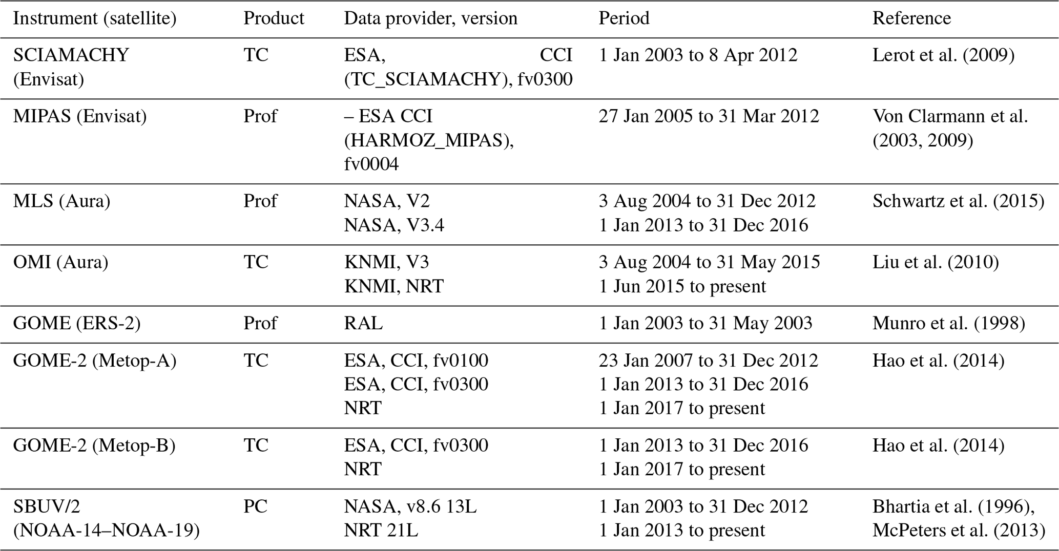
Table 3 Observations of ozone used in the CAMS-Rean assimilation system.

2.2 The CAMS Reanalysis

The CAMS Reanalysis (CAMS-Rean; Inness et al., 2019) is the successor of CAMS-iRean. Compared to CAMS-iRean, the horizontal resolution has increased to ∼80 km (T255), while meteorology is now based on CY42R1. Emissions are largely similar to CAMS-iRean, except that the monthly-varying biogenic emissions have been used for the full time period. With respect to the CB05-based chemistry module, heterogeneous chemistry on clouds and aerosol has been switched on, as well as the modification of photolysis rates due to aerosol scattering and absorption (Huijnen et al., 2014).

As for assimilated ozone observations, data from a very similar set of instruments have been used as for CAMS-iRean: SCIAMACHY, MIPAS, OMI, MLS, GOME-2, and SBUV/2; see Table 3. However, note that the CAMS interim Reanalysis additionally assimilated GOME profile observations during the first 5 months of 2003, which have not been assimilated in CAMS-Rean as it was found to lead to a degradation in the O₃ analysis. Different to CAMS-iRean, CAMS-Rean also assimilated observations from the MIPAS instrument during 2003 and early 2004, although using a different version. Also, frequently, newer versions of the data have been adopted in CAMS-Rean compared to CAMS-iRean. Particularly for MLS observations, the reprocessed version 4 has been applied throughout the full time period.

In CAMS-Rean also tropospheric NO₂ columns are assimilated, using observations from the SCIAMACHY (2003–2012), OMI (from October 2004 onwards), and GOME-2 (from April 2007 onwards) instruments. The same settings for the variational bias correction were used in CAMS-Rean as in CAMS-iRean.

CAMS-iRean and CAMS-Rean surface and tropospheric ozone are archived with a 3-hourly output frequency.

2.3 Tropospheric Chemistry Reanalysis (TCR-1)

The TCR-1 data assimilation system is constructed using an EnKF approach. A revised version of the TCR-1 data is used in this study. A major update from the original TCR-1 system (Miyazaki et al., 2015) to the system used here (Miyazaki et al., 2017; Miyazaki and Bowman, 2017) is the replacement of the forecast model from CHASER (Sudo et al., 2002) to MIROC-Chem (Watanabe et al., 2011), which caused substantial changes in the a priori field and thus the data assimilation results of various species.

MIROC-Chem considers detailed photochemistry in the troposphere and stratosphere by simulating tracer transport, wet and dry deposition, and emissions, and it calculates the concentrations of 92 chemical species and 262 chemical reactions. The MIROC-Chem model used in TCR-1 has a T42 horizontal resolution ($\sim {\mathrm{2.8}}^{\circ }$) with 32 vertical levels from the surface to 4.4 hPa. It is coupled to the atmospheric general circulation model MIROC-AGCM version 4 (Watanabe et al., 2011). The simulated meteorological fields were nudged toward the 6-hourly ERA-Interim (Dee et al., 2011) to reproduce past meteorological fields.

The a priori anthropogenic NO_x and CO emissions were obtained from the Emission Database for Global Atmospheric Research (EDGAR) version 4.2 (EC-JRC, 2011). Emissions from biomass burning were based on the monthly Global Fire Emissions Database (GFED) version 3.1 (van der Werf et al., 2010). Emissions from soils were based on monthly-mean Global Emissions Inventory Activity (GEIA; Graedel et al., 1993).

The data assimilation used is based on an EnKF approach (Hunt et al., 2007) that uses an ensemble forecast to estimate the background error covariance matrix and generates an analysis ensemble mean and covariance that satisfy the Kalman filter equations for linear models. The concentrations and emission fields of various species are simultaneously optimized using the EnKF data assimilation; see also Table 4.

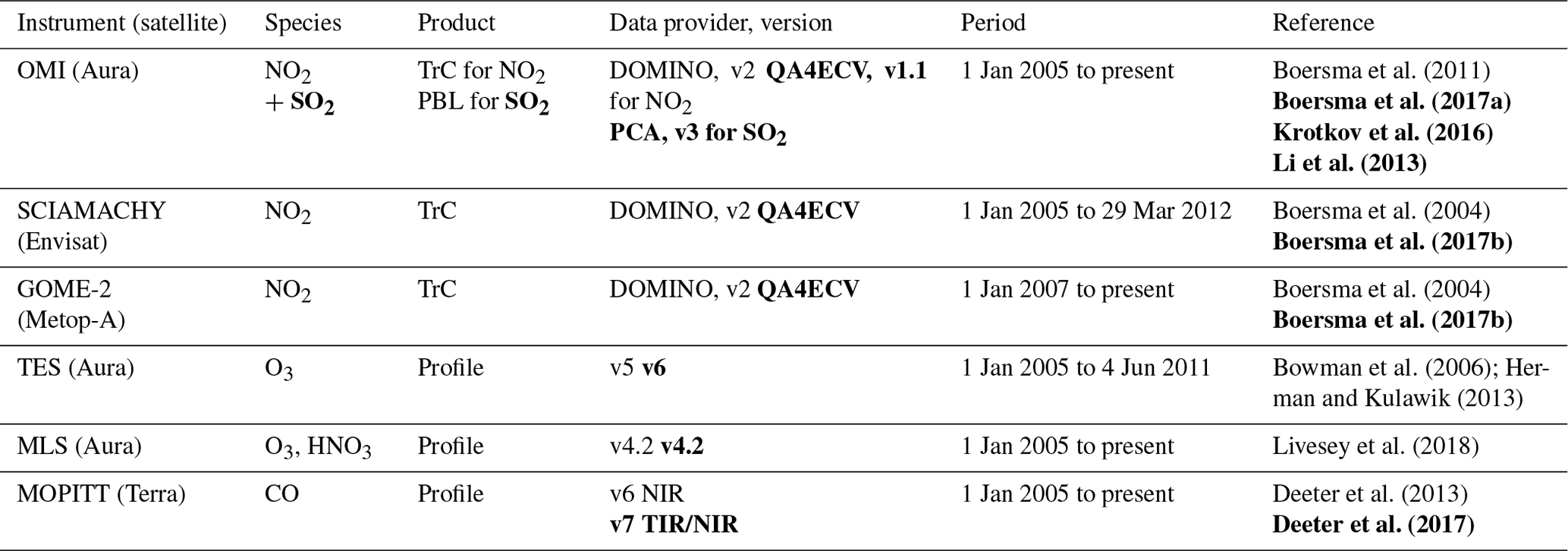
For data assimilation of tropospheric NO₂ column retrievals, the version 2 Dutch OMI NO₂ (DOMINO) data product (Boersma et al., 2011) and version 2.3 TM4NO2A data products for SCIAMACHY and GOME-2 (Boersma et al., 2004) were used, obtained through the TEMIS website (http://www.temis.nl, last access: 20 March 2020). The TES ozone data and observation operators used are version 5 level 2 nadir data obtained from the global survey mode (Bowman et al., 2006; Herman and Kulawik, 2013). TES ozone data were excluded poleward of 72^∘ because of the small retrieval sensitivity, limiting data assimilation adjustments at high latitudes in the troposphere. Also note that the availability of TES measurements is strongly reduced after 2010, which led to a degradation of the reanalysis performance, as demonstrated by Miyazaki et al. (2015). The MLS data used are the version 4.2 ozone and HNO₃ level 2 products (Livesey et al., 2018). Data for pressures of less than 215 hPa for ozone and 150 hPa for HNO₃ were used. The MOPITT CO data used are version 6 level 2 thermal-infrared retrieval (TIR) products (Deeter et al., 2013). A super-observation approach was employed to produce representative data with a horizontal resolution of the forecast model NO₂ and CO observations, following the approach by Miyazaki et al. (2012). No bias correction was applied to the assimilated measurements.

Table 4 Observations used for ozone assimilation in TCR-1, and changes for TCR-2 are shown in bold.

2.4 Updated Tropospheric Chemistry Reanalysis (TCR-2)

An updated chemistry transport model (CTM) and satellite retrievals are used in TCR-2 (Kanaya et al., 2019; Miyazaki et al., 2019, 2020; Thompson et al., 2019). A high-resolution version of the MIROC-Chem model with a horizontal resolution of T106 (${\mathrm{1.1}}^{\circ }\times {\mathrm{1.1}}^{\circ }$) was used. Sekiya et al. (2018) demonstrated the improved model performance on tropospheric ozone and its precursors by increasing the model resolution from ${\mathrm{2.8}}^{\circ }\times {\mathrm{2.8}}^{\circ }$ to ${\mathrm{1.1}}^{\circ }\times {\mathrm{1.1}}^{\circ }$. A priori anthropogenic emissions of NO_x and CO were obtained from the HTAP version 2 inventory for 2008 and 2010 (Janssens-Maenhout et al., 2015). Emissions from biomass burning are based on the monthly GFED version 4.2 inventory (Randerson et al., 2018) for NO_x and CO, while those from soils are based on the monthly GEIA inventory (Graedel et al., 1993) for NO_x. Emission data for other compounds are taken from the HTAP version 2 and GFED version 4 inventories.

The satellite products used in TCR-2 are more recent than those used in TCR-1; see Table 4. Tropospheric NO₂ column retrievals used are the QA4ECV version 1.1 L2 product for OMI (Boersma et al., 2017a) and GOME-2 (Boersma et al., 2017b). Version 6 of the TES ozone profile data was used. The MLS data used are the version 4.2 ozone and HNO₃ L2 products (Livesey et al., 2018). The MOPITT total column CO data used were the version 7L2 TIR/NIR product (Deeter et al., 2017). OMI SO₂ data of the planetary boundary layer vertical column L2 product were used as produced with the principal component analysis algorithm (Krotkov et al., 2016; Li et al., 2013). As in TCR-1, a super-observation approach to produce representative data with a horizontal resolution of the forecast model (${\mathrm{1.1}}^{\circ }\times {\mathrm{1.1}}^{\circ }$) for NO₂ and CO observations was applied. As in TCR-1, no bias correction was applied to the assimilated measurements.

TCR-2 data were used to study the processes controlling air quality in East Asia during the KORUS-AQ aircraft campaign (Miyazaki et al., 2019). Kanaya et al. (2019) demonstrated the TCR-2 ozone and CO performance using research vessel observations over open oceans. Thompson et al. (2019) used the TCR-2 data to help with the understanding of near-surface NO₂ pollution observed during the KORUS-OC campaign. Both for TCR-1 and TCR-2, the reanalysis data are archived on a 2-hourly output frequency.

2.5 Temporal consistency of the observing systems

Discontinuities in the observing systems, as specified in Tables 2–4, can cause significant temporal changes in the reanalyses quality. In 4D-Var systems this can be assessed through statistics based on analysis departures (observation minus analysis) and first-guess departures (observations minus model first guess). Inness et al. (2019) provide an extended overview of the biases of various assimilated observations against the CAMS Reanalysis. For ozone assimilation in particular, the following findings are most noteworthy for this study (see also Appendix C of Inness et al., 2019):

• There are larger biases for SCIAMACHY observations in 2003 and early 2004, associated with issues with the early SCIAMACHY O₃ retrievals in this time period.

• There are larger departures for MIPAS data during 2003–2004 than after 2005, where CCI data were used.

• There is a different behaviour of OMI data between 2009 and 2012, associated with a deterioration in the OMI row anomalies (Schenkeveld et al., 2017), which unfortunately have not be filtered out in the CAMS assimilation procedure.

• There is an increasing bias correction for GOME-2A, especially after January 2013, associated with a version change of the SBUV/2 data.

With respect to both TCR reanalyses, which are based on the EnKF approach, important information regarding the reanalysis product is provided by the error covariance. The analysis ensemble spread is estimated as the standard deviation of the simulated concentrations across the ensemble and can be used as a measure of the uncertainty of the reanalysis product (Miyazaki et al., 2012b). The uncertainty information on the analysis uncertainty is included in the TCR-1 and TCR-2 reanalysis products, and this can be used to investigate the long-term stability of the data assimilation performance. In addition, the χ² test was used to evaluate the temporal changes in data assimilation balance (e.g. Ménard and Chang, 2000). Miyazaki et al. (2015) demonstrated increased χ² for OMI NO₂ after 2010, associated with a decrease in the number of the assimilated measurements and changes in the super-observation error due to the OMI row anomalies. Furthermore, the decreased number of assimilated TES ozone retrievals after 2010 affected the long-term reanalysis characteristics. Before 2011 the analysis spread for ozone in the middle troposphere is about 1–3 ppb in the tropics and subtropics and 3–12 ppbv in the extratropics. The larger spread at lower latitudes could be attributed to the higher sensitivities in the TES ozone retrievals. From 2011 onwards the spread mostly becomes smaller than 3 ppb for the globe, which seems excessively small and is likely associated with the lack of effective observations for measuring the analysis uncertainties and with the stiff tropospheric chemical system. The obtained results indicate the requirements for additional observational information and/or stronger covariance inflation to the forecast error covariance for measuring the long-term analysis spread corresponding to actual analysis uncertainty.

3 Ozone observations used for evaluation

3.1 Ozone-sondes

For evaluation of free-tropospheric ozone data from the global network of ozone-sondes, as collected by the WOUDC, is used, as these are expanded with observations available from SHADOZ (Thompson et al., 2017; Witte et al., 2017) and ESRL. The observation error of the sondes is about 7 %–17 % below 200 hPa and ±5 % in the range between 200 and 10 hPa (Beekmann et al., 1994; Komhyr et al., 1995; Steinbrecht et al., 1998). Typically, the sondes are launched once a week, but, in certain periods such as during ozone hole conditions, launches can be more frequent. Sonde launches are mostly carried out between 09:00 and 12:00 LT (local time).

The ozone-sonde network provides a critical independent validation of the reanalysis products. Although the number of soundings varied for the different stations, the global distribution of the launch sites is expected to be sufficient to allow for meaningful monthly-to-seasonal averages over larger areas. However, because of the sparseness of the ozone-sonde network, we are aware that the evaluation based on ozone-sonde observations can introduce large biases in regional and seasonal reanalysis performance (Miyazaki and Bowman, 2017).

The reanalysis data have been co-located with observations through interpolation in time and space. Individual intercomparisons have been aggregated on a monthly and seasonal basis. The number of stations contributing to the monthly and regional means varies over the course of the reanalysis products, and it is additionally reported as this is naturally an important consideration when assessing interannual variability of ozone biases. While we present time series from 2003 onwards in our figures, where CAMS starts to provide reanalysis products, for any of the statistics we only base this on the 2005–2016 time period (unless explicitly mentioned) to allow for fair intercomparison between CAMS and TCR.

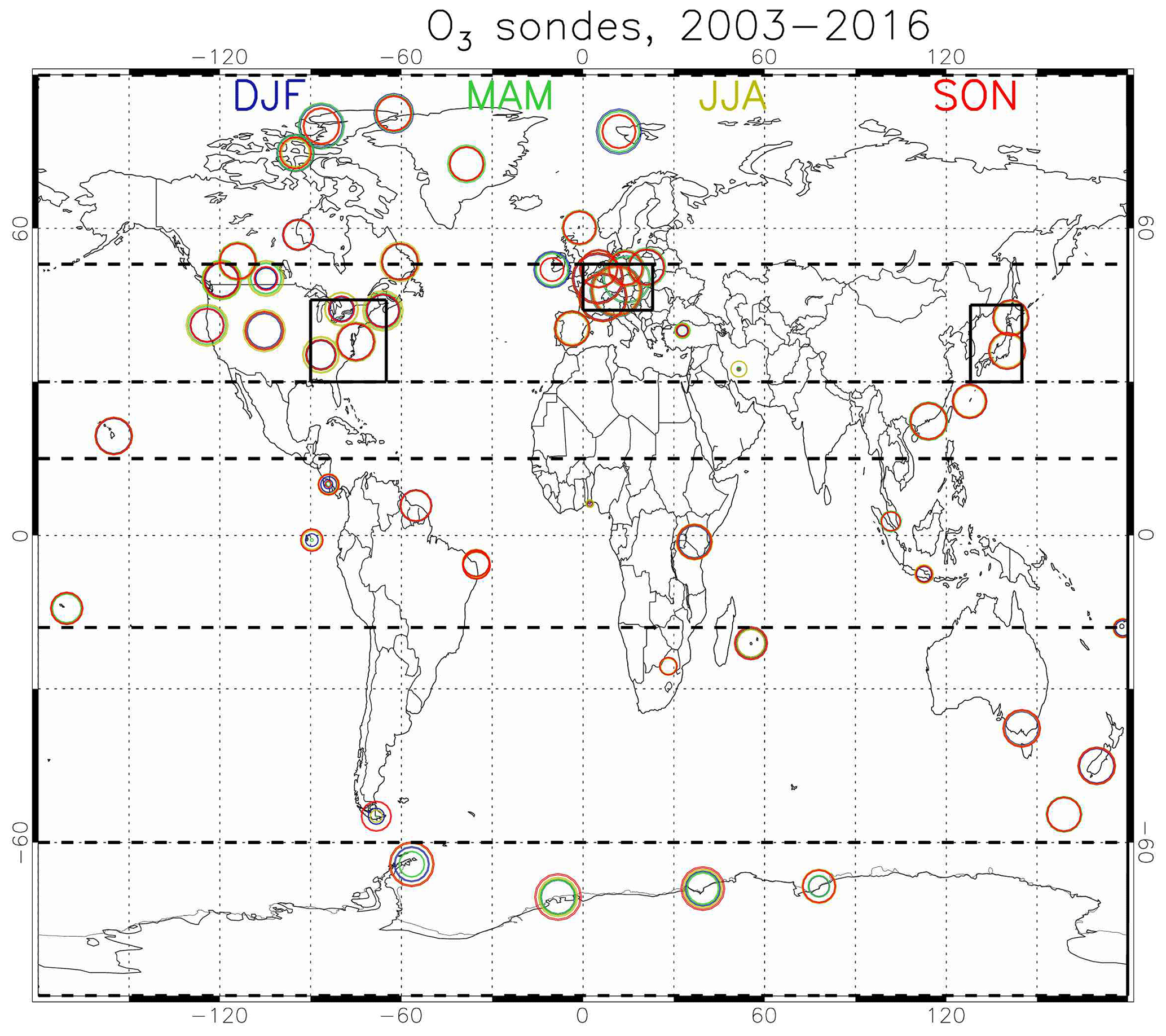
Figure 1 Locations of ozone-sondes contributing to the various regions. The size of circles indicates the relative number of observations contributing to the statistics for December–February (blue), March–May (green), June–August (yellow), and September–November (red). The dashed lines indicate the latitude bands representing the NH arctic region (53–90^∘ N), NH mid-latitudes (30–53^∘ N), NH subtropics (15–30^∘ N), tropics (18^∘ S–15^∘ N), SH mid-latitudes (60–18^∘ S), and Antarctic regions (90–60^∘ S). The black boxes indicate three additional regions in the NH mid-latitudes: eastern US (90–65^∘ W, 30–46^∘ N), western Europe (0–23^∘ E), and Japan (30–45^∘ N, 128–145^∘ E).

For spatial aggregation, the choice is more difficult, depending on the characteristics of the species and availability of observations. Tilmes et al. (2012) defined an aggregation approach for ozone-sonde locations based on the characteristics of the observed ozone profiles. We follow in part their aggregation approach, by adopting the European, eastern US, Japan, and Antarctic regions. For several regions, the number of measurements could be insufficient to construct meaningful aggregates. Instead we define regions for the Northern Hemisphere (NH) subtropics, the tropics, Southern Hemisphere (SH) mid-latitudes and Antarctica, and we combine the NH polar regions into a single region; see also Fig. 1.

3.2 Surface ozone

We evaluate surface ozone against the TOAR database (Schultz et al., 2017b), which provides a globally consistent, gridded, long-term dataset with ozone observation statistics on a monthly-mean basis. The TOAR database has been produced with particular attention to quality control, and representativeness of the in situ observations, in order to establish consistent, long-term time records of observations. TOAR provides a disaggregation of rural and urban stations. For our study, we use the ${\mathrm{2}}^{\circ }\times {\mathrm{2}}^{\circ }$ gridded monthly-mean dataset representative of rural stations for the 1990–2014 time period. This allows for easy intercomparison with monthly-mean results from the various reanalysis products.

Note that in these comparisons we used rural observations only, because none of the reanalysis model resolutions are considered sufficient to resolve local concentration changes over highly polluted urban areas. Therefore, the rural observations can be considered as more representative data for grid averaged concentrations. Nevertheless, neglecting urban observations could lead to biased evaluations particularly in cases where large fractions of the grid cells are associated with urban conditions, e.g. in megacities.

This TOAR dataset has a good global coverage, including stations over East Asia, and provides overall a constant and good quality controlled data record up to 2014. Nevertheless, the number of records in this database decreases significantly for various regions on the globe after 2012. Therefore, in our evaluation statistics, we focus on the period before 2012, considering that the reduction in available observations afterwards hampers the intercomparison of reanalysis performance between different years. Similar to the evaluation against ozone-sonde observations, the statistics are computed for data from 2005 onwards.

3.3 EMEP observations

In order to assess the ability of the reanalysis products to represent spatial and temporal variability on a sub-seasonal and on regional scales, we additionally evaluate the reanalyses against ground-based hourly observations from the EMEP network (obtained from http://ebas.nilu.no/, last access: 20 March 2020) for the year 2006. Although EMEP data are also included in the TOAR data product, this analysis allows for a complementary approach, in particular the assessment of pollution events during heatwaves but also evaluation of the diurnal cycles and spatial variability in the various products. The summer period of 2006 over Europe was characterized by a heatwave event (Struzewska and Kaminski, 2008). For this evaluation, we co-locate the reanalysis output spatially and temporally to the observations, using a reference 3-hourly time frequency. Considering the comparatively coarse horizontal resolution, which is not generally able to represent the local orography at the location of the individual observations, we match the model level with the same (average) pressure level at the location of the observations. Here we note that the CAMS reanalyses use a higher vertical resolution than TCR. This implies that for high-altitude stations also different (higher) model levels are sampled in the CAMS reanalyses compared with TCR. After this co-location procedure, we compute temporal correlation coefficients on a seasonal basis, using the temporally co-located 3-hourly reanalysis and observational data.

4 Evaluation against ozone-sondes

4.1 Annually and regionally averaged profiles

Figure 2 provides an overview of the multiannual mean ozone for the four reanalyses for the 2005–2016 time period. All reanalyses capture the observed vertical profiles of ozone from the lower troposphere to the lower stratosphere, with a regional mean bias of typically less than 8 ppb throughout the troposphere. Corresponding mean biases at 850, 650, and 350 hPa are given in Fig. 3, where the bias is defined as the reanalysis minus observation throughout this work. The normalized values, as scaled with the mean of the observations, are given in Fig. S1 in the Supplement. These multiannual, regional mean biases are below 3.7 ppb at 850 hPa and 4 ppb at 650 hPa, while normalized (absolute) biases are mostly below 10 %. For most regions, the CAMS Reanalysis shows improvement against the CAMS interim Reanalysis at 650 hPa and also 850 hPa, particularly for regions over the NH middle and high latitudes, as well as the SH mid-latitudes, but at the cost of a degradation (an emerging positive bias) towards the surface. TCR-2 shows a more mixed picture in this respect. Biases between TCR and CAMS are within a similar order of magnitude, but they are not correlated in any way in sign or magnitude. For most of the major polluted areas in the lower troposphere, the biases are lower in the CAMS Reanalysis than in the TCR reanalyses, probably due to its higher reanalysis model resolution and a better chemical forecast model performance. The annual mean ozone biases in TCR are relatively large in the tropics and SH high latitudes. After 2011, no TES tropospheric ozone measurements were assimilated, which could lead to enhanced ozone biases, as demonstrated by Miyazaki et al. (2015). Assimilation of MLS measurements does not noticeably influence the tropospheric ozone analysis in the tropics. In the NH subtropics and tropics regions the reanalyses show some larger deviation against sonde observations at lower altitudes, which was traced to comparatively large biases at the Hong Kong and Kuala Lumpur stations. Note that in these regions the ozone-sonde network is sparse, while the spatial and temporal variability of ozone is large, which limits our understanding of the generalized reanalysis performance (Miyazaki and Bowman, 2017). At high latitudes, the large diversity in the reanalysis ozone could be associated with the lack of direct tropospheric ozone measurements in all of the systems.

Overall, this evaluation shows that the biases from these reanalysis products are smaller than those reported from recent CTM simulations. For example, Young et al. (2013) present median biases across ACCMIP model versions at 700 (500) hPa up to 10 (15) %, depending on the region. This demonstrates that the reanalysis of tropospheric ozone fields is generally well constrained by assimilated measurements for the globe.

Figure 2 Evaluation of regional mean multiannual mean O₃ profiles against ozone-sondes, averaged over the 2005–2016 time period.

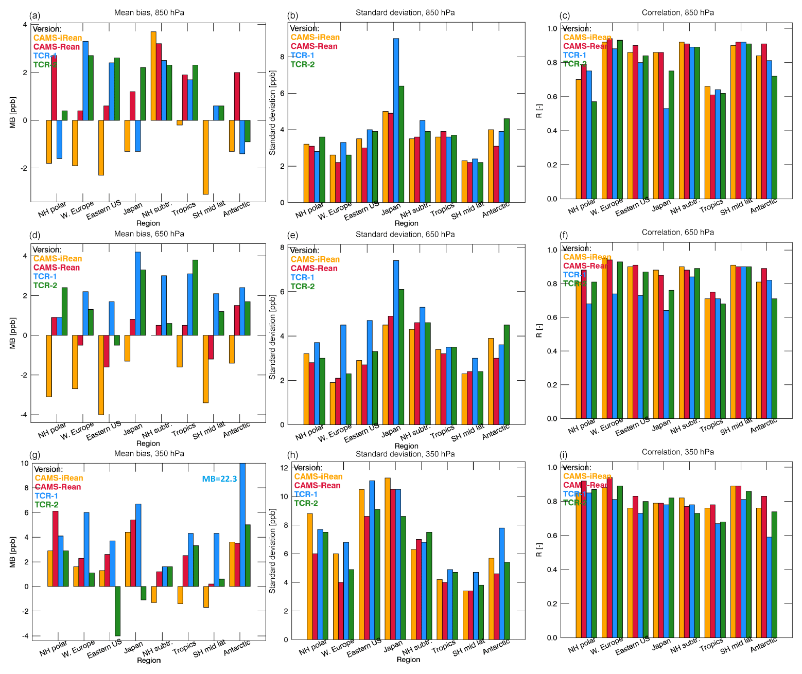
Figure 3 Evaluation of ozone mean bias (reanalysis minus observation, a, d, g), standard deviation of the unbiased differences (b, e, h), and temporal correlation R (c, f, i) for the four reanalysis products at 850 (a–c), 650 (d–f), and 350 (g–i) hPa against sondes, computed for various regions, for the 2005–2016 time period.

4.2 Time series of zonally averaged O₃ tropospheric columns

Co-located partial columns from the surface up to 300 hPa, hereafter for brevity referred to as “tropospheric columns”, have been compared to partial columns derived from the sonde observations. An intercomparison of the monthly and zonally mean tropospheric columns sampled at the observations is given in Fig. 4. The corresponding performance statistics are given in Fig. 5. Here, the standard deviation (SD) is computed based on the unbiased differences between the reanalyses and sonde observations, and it provides a metric of the quality of the monthly-mean variability in the reanalyses.

Normalized statistics are provided in Fig. S2. Note that the figures also contain information on the number of sonde stations that are included in the evaluation for individual months.

Outside the polar regions all reanalyses capture the magnitude of the zonal mean tropospheric column to within a mean bias (MB) of within 1.8 DU, and the SD is between 0.8 and 1.3 DU depending on the reanalysis product. For most regions and performance metrics, the updated reanalyses outperform their predecessor versions. For instance, for the NH mid-latitudes, the MB is −0.3 DU (1.2 %, when normalized with sonde observations) for CAMS-Rean and 0.8 DU (3 %) for TCR-2, which were earlier −1.2 DU (CAMS-iRean) and 1.8 DU (TCR-1).

Largest uncertainties are found for the polar regions, with MB within 2.6 DU and the SD ranging from 1.4 (CAMS-Rean) to 2.1 DU (TCR-1), corresponding to up to ∼12 % of the average O₃ tropospheric column. Over the SH mid-latitudes the reanalyses show similar features as over the Antarctic region, with normalized mean biases within the range of −1 DU (−5 %, CAMS-iRean) to 1.5 DU (+10 %, TCR-1). The normalized standard deviations over the SH mid-latitudes are within 7 %, marking a considerably better ability to capture temporal variability than over the Antarctic region.

In the tropics the MB ranges from −0.6 to 1.2 DU, and the SD is about 1.0 DU, or ∼5 % of the average O₃ tropospheric column. The temporal correlation between analysed and observed tropospheric columns is correspondingly highest (R>0.90) for the NH mid-latitudes but still relatively low for the Antarctic region (R<0.80) for all reanalyses. This relatively poor temporal correlation over the Antarctic region, despite the strong seasonal cycle, does indicate difficulties of the reanalyses to reproduce a consistent seasonality over the full time series, as described in more detail in the following sections.

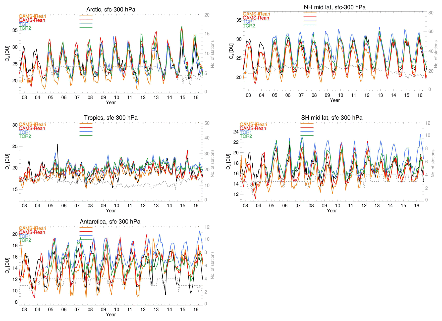
Figure 4 Evaluation of zonally averaged monthly-mean partial columns (surface to 300 hPa) against sonde observations. Observations are in black. The dashed grey line refers to the number of stations that contributes to the statistics (right vertical axis).

Figure 5 Analogous to Fig. 3 but for partial columns from surface to 300 hPa in Dobson units (DU).

4.3 Time series of regionally averaged O₃ biases at multiple altitudes

Figure 6 shows time series of monthly-mean ozone biases against ozone-sondes at three pressure levels (∼850, 650, and 350 hPa), aggregated for the predefined regions. The panels in this figure give an indication of the stability of the reanalyses against sonde observations during the 2003–2016 time period. The corresponding time series with monthly-mean concentration values, showing the seasonal cycle, is given in Fig. S3. As in the previous section, persistent changes in the number of stations may contribute to changes in biases over the course of the 14-year time interval. The mean bias, SD, and temporal correlation for each of these time series are given in Fig. 3. Based on these evaluations we note the following: over the NH polar region, CAMS-Rean shows a small, positive bias in the lower troposphere (2.7 ppb at 850 hPa for the 2005–2016 multiannual mean), particularly during the springtime (5.0 ppb when averaged over March–May). During 2003 and 2004 both CAMS reanalyses show anomalously low springtime ozone, different to the rest of the time period, particularly at ∼350 hPa. The different reanalysis performance statistics over the Arctic compared to later years is attributed to the use of early SCIAMACHY and NRT MIPAS O₃ retrievals, which are of poorer quality than the OMI MLS observations, which have been used from August 2004 onwards, and reprocessed MIPAS data used from January 2005 onwards. Combined with total column retrievals, assimilation of such stratospheric profiles has been shown to also affect the tropospheric contribution (Inness et al., 2013). CAMS-iRean shows a large offset compared to observations and CAMS-Rean in 2003, particularly at altitudes below 650 hPa. This was attributed to the assimilation of GOME nadir profiles in CAMS-iRean, which has been omitted in CAMS-Rean (Inness et al., 2019).

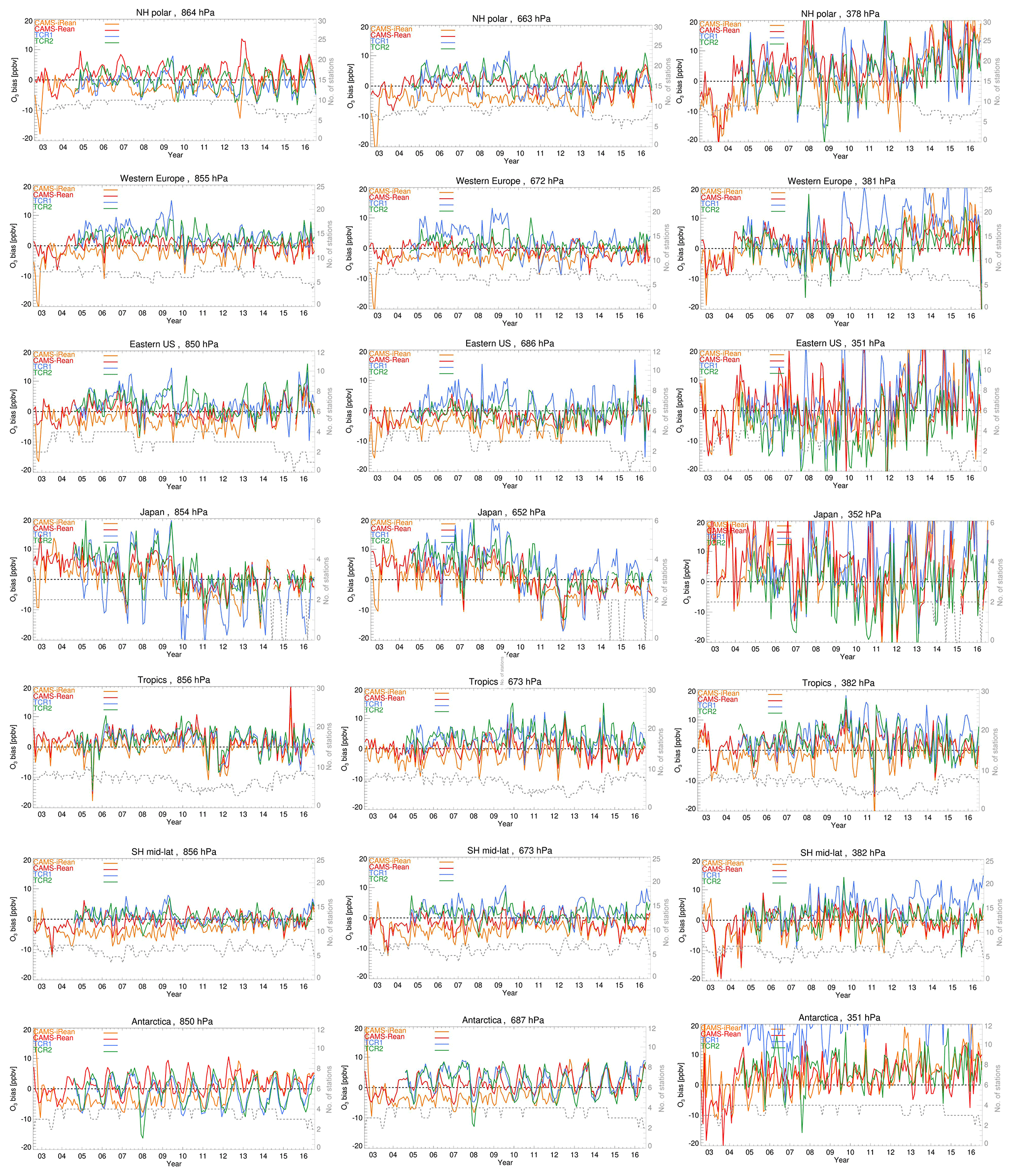
Figure 6 Time series of regionally and monthly aggregated ozone biases at different altitudes (850, 650, and 350 hPa) sampled at ozone-sonde locations. As in Fig. 4, the dashed grey line refers to the number of stations that contribute to the statistics (right vertical axis).

Furthermore, before 2014 CAMS-iRean shows lower values than CAMS-Rean, while for 2014 to 2016 the two CAMS reanalyses are much more alike. This offset before 2014 results in a slight negative bias against observations at ∼850 hPa over the Arctic, and a significant negative bias at ∼650 hPa, and it is attributed to the use of a different version of the MLS retrieval product from V2 to V3.4 (Flemming et al., 2017). The TCR reanalyses underestimate the lower tropospheric ozone after 2011, which could be associated with the lack of TES measurements during the recent years. At higher altitudes (650 and 350 hPa) differences between the reanalyses are relatively smaller. On average at 650 hPa CAMS-iRean shows a slight underestimation (−3.1 ppb), while CAMS-Rean and TCR-1 bias is below 1 ppb and slightly larger for TCR-2 (2.4 ppb). At 350 hPa all reanalysis products perform overall similar. At this altitude a considerable interannual variability is visible in the observations (see Fig. S3), which appears to be well captured by the reanalysis products, with temporal correlations in the order of R=0.85 (for TCR-1) to R=0.92 (for CAMS-Rean). Also both the observations and reanalyses indicate an upward trend of tropospheric ozone in the Upper Troposphere–Lower Stratosphere (UTLS), as also confirmed by Williams et al. (2019).

Over western Europe the CAMS reanalyses show good correspondence to the observations at 850 hPa from 2004 onwards, with mean biases of −1.9 (CAMS-iRean) and 0.4 ppb (CAMS-Rean). The TCR reanalyses overestimate ozone at lower altitudes, particularly in TCR-1 before 2010, which shows positive biases at 850 hPa of up to ∼15 ppb, with an average over the full time period of 3.3 ppb. Such overestimates suggest a strong influence of the forecast model performance for the boundary layer (e.g. mixing and chemistry), while the optimization of the emission precursors was not sufficient to improve the lower tropospheric ozone analysis. At ∼650 and ∼350 hPa, the reanalyses reproduced well the observed seasonal and interannual variations. As an exception, TCR-1 overestimates ozone for some cases, especially in winter. In contrast, the CAMS reanalyses show average (absolute) biases of less than 3.3 ppb at all pressure levels.

Over the eastern US, all the reanalysis products show similar SD values at ∼850 hPa (3.0–4.0 ppb), which is associated with positive analysis biases, mostly during summer by 0.3–6.8 ppb. Such biases have also been reported in dedicated studies (e.g. Travis et al., 2016), which could be associated with model errors, e.g. excessive vertical mixing and net ozone production in the boundary layer. The annual mean bias for the reanalyses ranges between −2.3 and 2.6 ppb. A decrease in the observed ozone concentrations at ∼850 hPa after 2014, associated with a change in the number of contributing stations in this evaluation, leads to a general and consistent overestimate in all of the reanalyses. A similar agreement with the observations was found in the middle troposphere compared to the lower troposphere, with SD ranging between 2.9 and 4.7 ppb, while at ∼350 hPa the SD ranges between 8.6 and 11.1 ppb.

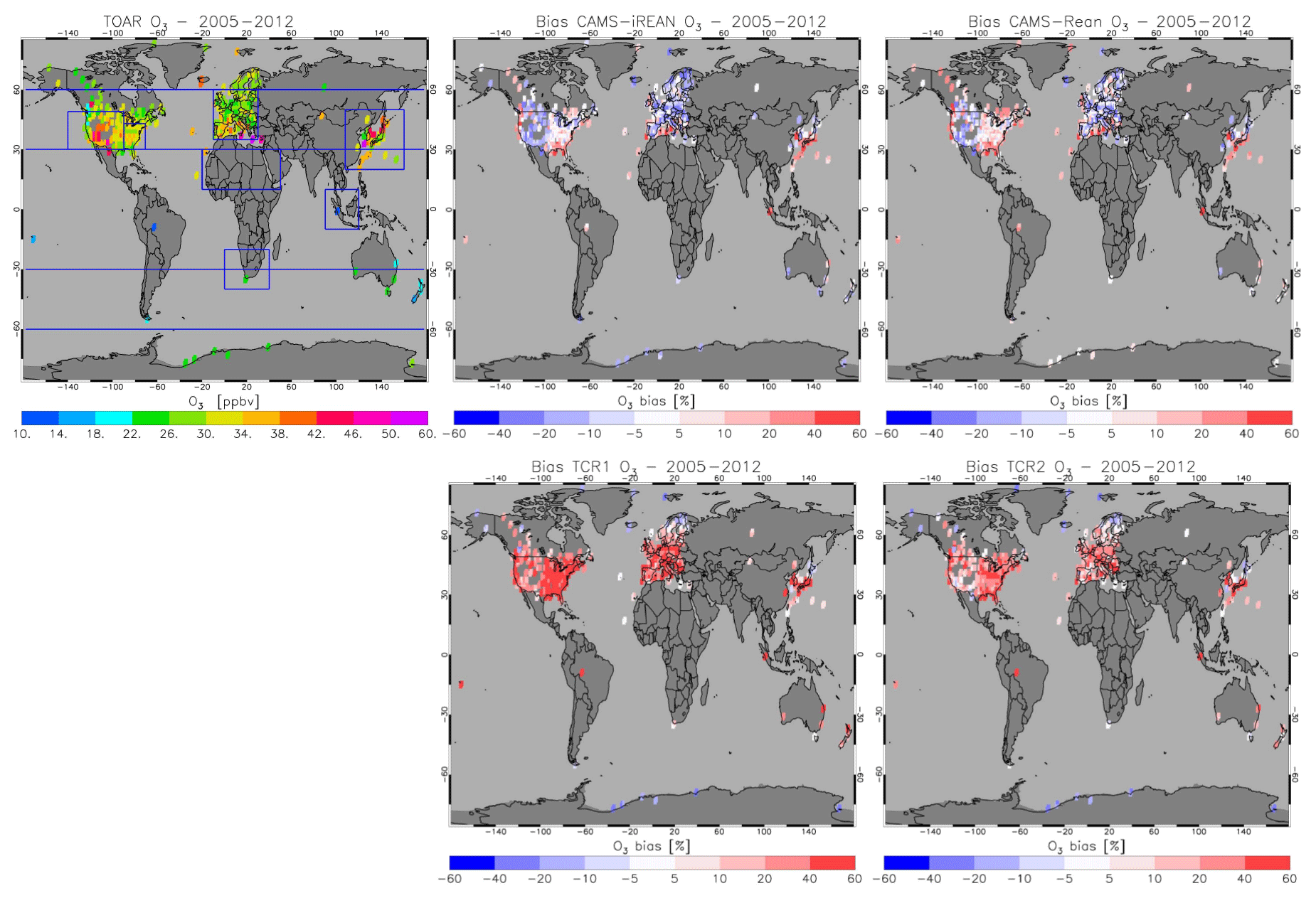
Figure 7 Multiannual (2005–2012) mean surface ozone from TOAR (upper left), along with corresponding normalized mean bias with respect to the observations for the reanalyses.

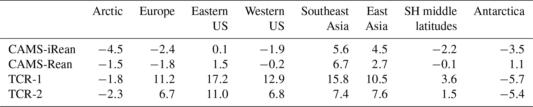
Table 5 Mean bias (ppb) for the reanalyses against TOAR monthly mean and regional mean observations for the 2005–2012 time period, as sampled for observations in the specified regions indicated in Fig. 7.

Over Japan, all reanalyses on average overestimate ozone at 850 and 650 hPa before 2011, with relatively large, positive biases in TCR-1 and TCR-2 at 650 hPa (7.9 and 6.9 ppb, respectively, when averaged for the 2005–2010 time period). From 2011 onwards the correspondence with observations improves remarkably. The changes in performance statistics for all reanalyses likely have multiple causes. This includes trends in the observed ozone (Verstraeten et al., 2015), associated with changes in Chinese precursor NO_x emissions (e.g. van der A et al., 2017). Also changes in the observing system are important to consider, particularly the reduction of assimilated TES measurements in TCR from 2010 onwards and the row anomaly issues affecting assimilated OMI O₃ and NO₂; see also Sect. 2.5.

In the tropics, all reanalyses except CAMS-iRean overestimate ozone at 850 hPa before 2012, with positive biases in the range 2.5–3 ppb. The different performance for CAMS-iRean from 2012 onwards is probably associated with the use of another version of the MLS retrieval product. Interestingly, both CAMS reanalyses show a strong peak in ozone at 850 hPa during the second half of 2015 (see corresponding Fig. S3) but with a zonally averaged overestimation of up to 20 ppb. This is associated with the strong El Niño conditions, and this particular spike was attributed to an overestimate of ozone observed at the Kuala Lumpur station for October 2015. Here exactly the grid box affected by the extreme fire emissions in Indonesia for this period (Huijnen et al., 2016), as prescribed by the daily GFAS product, has been sampled. This peak appears much weaker in TCR. Possible explanations are lower optimized NO_x and CO emissions in TCR compared to those used in CAMS, resulting in weaker ozone production, together with a coarser reanalysis model resolution. At 650 hPa, the TCR reanalyses overestimate ozone almost throughout the reanalysis period (by 3.1–3.8 ppb on average), whereas the CAMS-Rean shows closer agreement with the observations (MB = 0.5 ppb, SD = 3.2 ppb). At ∼350 hPa, the TCR-2 shows improved agreement compared with the earlier TCR-1, as confirmed by improved mean bias (from 4.3 to 0.6 ppb) although with a similar SD (from 4.9 to 4.7 ppb). Also the temporal correlation remains relatively low.

Over the SH mid-latitudes an overall good correspondence is obtained for all reanalyses, but particularly CAMS-Rean and TCR-2, throughout the troposphere. This is marked by the lowest magnitudes for SD and highest for the temporal correlations for any of the three altitude ranges compared to the statistics in other regions. Nevertheless, CAMS-iRean still underestimates ozone before 2012 in the lower and middle troposphere, whereas TCR-1 overestimates it particularly at 382 hPa after 2010. Furthermore, CAMS-iRean and CAMS-Rean suffer from relatively large negative biases before 2005, particularly at 382 hPa. This is attributed to similar causes as have been discussed for the Arctic region.

A large diversity among the system performance is seen over the Antarctic region. As in the Arctic region, free-tropospheric O₃ in the CAMS reanalyses is comparatively poorly constrained during 2003, as a consequence of the use of the NRT data product from MIPAS and early SCIAMACHY data in the assimilation. Also in the period between the end of March and the beginning of August 2004 no profile data were available for assimilation, leading to a temporary degradation in the reanalysis performance.

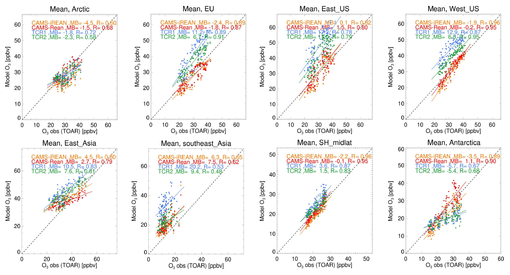
Figure 8 Scatter plot of surface ozone against TOAR observations for the 2005–2012 regionally averaged monthly-mean time series. The mean bias and temporal correlation are also given.

Before 2013, CAMS-iRean underestimates the low ozone values in the lower and middle troposphere during austral spring, while CAMS-Rean overestimates it during austral winter. Afterwards, both systems show very similar results, also in overall better agreement with the observations, even though an overestimate during austral spring remains. Reasons for the change in behaviour in CAMS-iRean is the change in MLS version from V2 to V3.4 after 2012. Furthermore both CAMS-iRean and CAMS-Rean are affected by a change from 6L SBUV to 21L NRT data in January and July 2013, respectively, which appears to contribute significantly to the changes in the bias. The seasonal cycle in the biases can largely be attributed to the lack of O₃ total column observations during polar night, combined with a seasonal variation in model forecast biases. The TCR reanalyses largely underestimate ozone during austral summer and autumn in the lower troposphere. At 351 hPa, TCR-1 substantially overestimates ozone throughout the year (22 ppb on average) because of large model biases and the lack of observational constraints. This large, positive bias was resolved in TCR-2 by improving the modelling framework.

In conclusion, evaluation of the tropospheric ozone reanalyses against ozone-sondes has revealed the following:

• The updated reanalyses show on average improved performance compared to the predecessor versions but with some notable exceptions, such as an increased positive bias over the Antarctic region in CAMS-Rean versus CAMS-iRean. Over the Antarctic region the TCR-2 strongly improved upon TCR-1, despite the lack of direct observational constraints.

• For individual regions or conditions, CAMS Reanalysis and TCR-2 show different performances but averaged for all regions of similar quality. Best performance, in terms of mean bias, standard deviation, and correlation, for the updated reanalyses is obtained for the western Europe, eastern US, and SH midlatitude regions (both normalized mean bias and standard deviation below 8 % at 850 and 650 hPa). Relatively worst performance is found for the Antarctic region, with normalized standard deviation up to 18 %. This is likely associated with the fewer observational constraints in the polar regions compared to the other regions.

• In terms of temporal consistency, the CAMS reanalyses show degraded performance over the polar regions during 2003 and 2004, due to lower quality MIPAS and SCIAMACHY data usage. CAMS-iRean also shows a change in performance statistics in the polar regions from 2014 onwards, associated with changes in the MLS retrieval product versions. Furthermore, both CAMS-Rean and CAMS-iRean are affected by the change in the SBUV/2 product versions in 2013.

With the reduced data availability from TES from 2010 onwards, the TCR tropospheric ozone products show changes in their performances. Remarkably, TCR-1 and TCR-2 show overall slight improvements from 2010 onwards. This is marked by reduced positive biases in the lower troposphere over NH mid-latitude regions and may be attributed to biases in the TES retrieval product, combined with changes in the OMI product; see also Sect. 2.5. Additional observing system experiments (OSEs) are needed to identify the relative roles of individual assimilated measurements on the changes in reanalysis bias.

Figure 9 Time series of regional monthly-mean ozone anomalies against those derived from the TOAR observations. The dashed line indicates the number of TOAR ${\mathrm{2}}^{\circ }\times {\mathrm{2}}^{\circ }$ grid boxes that contribute to the statistics. The temporal correlation as computed for the 2005–2014 time series is also given.

5 Validation against TOAR surface observations

We evaluated the reanalyses against monthly-mean gridded surface observations filtered for measurements performed at rural sites, as compiled in the TOAR project (Schultz et al., 2017b). These evaluations reveal the ability of the reanalysis products to reproduce near-surface background ozone concentrations in terms of mean value and variability, both temporally (on seasonal to annual timescales) and spatially for various regions over the globe.

5.1 Multiannual mean

Figure 7 shows a map with multiannual mean ozone observations from the TOAR database for the 2005–2012 time period, as well as the corresponding normalized biases in surface ozone for the reanalysis products. Detailed maps for North America, Europe, and East Asia are given in Fig. S4, while the corresponding regional mean biases are given in Table 5.

The TCR reanalyses show significant positive biases for many regions, with multiannual mean biases of 11.0 ppb and 6.8 ppb over the eastern and western US, respectively, and 6.7 ppb over Europe in TCR-2. These biases can mainly be attributed to model errors. Mean biases in the CAMS reanalyses are generally smaller (1.5 and −0.2 ppb for eastern and western US, respectively, and −1.8 ppb for Europe), but they still show substantial spatial variations, as quantified by the root mean square of the multiannual mean differences across the various regions, which is 8.9 and 6.1 ppb for eastern and western US, respectively, and 5.6 ppb over Europe for the CAMS Reanalysis (18, 11, and 11 ppb for TCR-2 for these regions). The mean bias is negative over the Arctic, Europe, and western US, and it is positive over East Asia and Southeast Asia in both versions of the CAMS reanalyses. The positive regional mean biases over the major polluted regions are reduced by 35 % to 55 % in TCR-2 as compared with TCR-1. Likewise, the negative biases over the Arctic, Europe, western US, and SH middle and high latitudes are reduced by more than 25 % in CAMS-Rean as compared with CAMS-iRean, illustrating overall improvements for the newer reanalyses.

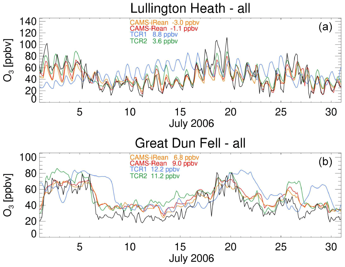
Figure 10 Time series of reanalyses against ozone observations at two EMEP stations in Great Britain during July 2006: Lullington Heath (a, 120 $\mathrm{m}\mathrm{a}.\mathrm{s}.\mathrm{l}.$, model levels 3 (CAMS) and 1 (TCR)) and Great Dun Fell (b, 847 $\mathrm{m}\mathrm{a}.\mathrm{s}.\mathrm{l}.$, model levels 8 (CAMS) and 3 (TCR)). Also given are mean biases.

5.2 Variability in regionally averaged surface ozone

Figure 8 presents scatter plots of monthly-mean ozone (2005–2012) from the reanalyses against those from the TOAR surface observations for various regions. The corresponding time series, given in Fig. S5, indicate that the main driver of the variation in magnitude of ozone concentrations in the reanalyses and observations is associated with the seasonal cycle. Over the Arctic, the general pattern in the monthly variations is captured for all reanalyses (R between 0.58 and 0.72), although they all underestimate the increased ozone values during boreal spring.

Over Europe and the US, the CAMS reanalyses show the closest agreement with the observations (MB between −2.4 and 1.5 ppb, R>0.8). CAMS-Rean shows improved negative biases for observed low ozone values compared with the CAMS-iRean, which is in boreal winter and spring. The TCR reanalyses exhibit large, positive biases over Europe and the US regions (MB between 6.7 and 17 ppb), with significant improvements in TCR-2. Over East Asia, all the reanalyses show positive biases in the range of 2.7 ppb (CAMS-Rean) to 10.5 ppb (TCR-1) and fail to reproduce the minimum concentrations in autumn. Still the temporal correlations are similar to most other regions (R between 0.79 and 0.83), associated with the stable seasonal cycle in both the reanalyses and observations. Over Southeast Asia, positive biases exist throughout the period, which are largest in TCR-1. For this region, the TCR reanalyses show lower temporal correlations (R between 0.39 and 0.49) compared to the CAMS reanalyses (R=0.68).

Significant changes in the surface ozone biases are found in the TCR reanalyses over the SH mid-latitudes, with reduced positive biases after 2010. The CAMS reanalyses capture well the temporal variability over the SH mid-latitudes and Antarctic region (R between 0.89 and 0.96), while CAMS-Rean shows a positive bias for observed high ozone values. This is associated with model biases in austral winter (JJA), particularly during 2005–2013 (Fig. S5). The TCR reanalyses show a significant negative bias throughout the year except for observed low ozone values (during Austral summer), which result in lower temporal correlations (R≈0.68).

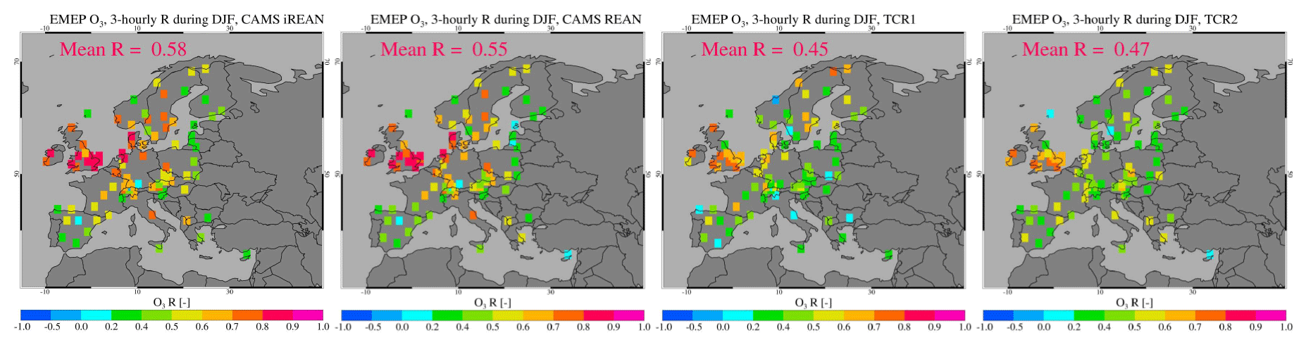
Figure 11 Correlation coefficients computed for 3-hourly DJF 2006 at EMEP stations for the four reanalyses. The mean value, based on correlations computed for all individual stations, is given.

Figure 12 As Fig. 11 but for JJA.

The free-tropospheric intercomparison at different altitudes, as presented in Fig. 3, already indicated generally larger biases at 850 hPa compared to 650 hPa. This can be understood as near-surface ozone concentrations that are less well constrained by the satellite data products used in the assimilation, and they depend strongly on local conditions such as precursor emissions, deposition, vertical mixing, and chemistry, which are difficult to parameterize at the model grid scale (Sekiya et al., 2018).

An important example of a driver for local variability is the emissions from forest fires, which in the CAMS reanalyses are provided through daily-varying GFAS emissions. This has been shown to capture to a good degree the carbon monoxide and aerosol from fire plumes, although larger uncertainties exist in the NO_x emissions, e.g. Bennouna et al. (2019).

In summary, CAMS-Rean shows the best ability to capture the regional mean surface ozone and its variability, while particularly TCR-2 (and to a lesser extent also TCR-1) shows positive biases and reduced correlations. Particularly good performance is seen over the western US (R=0.95, $\text{MB}=-\mathrm{0.2}$), while over eastern, and particularly southeast, Asia the performance is poorest.

Figure 13 Plots of seasonal mean diurnal cycle against EMEP observations for 2006. Central Europe is here defined as the region between 35 and 45^∘ N, with northern (southern) Europe at higher (lower) latitudes. Note that the reanalysis bias has been removed. Model level selection is through matching of the reanalysis pressure with pressure level of the station sites.

5.3 Interannual variability of regionally averaged surface ozone

We assess the interannual variability (IAV) by computing the de-seasonalized anomaly of surface ozone concentrations. For this, the 2005–2012 multiannual monthly, regional mean surface ozone is subtracted from its corresponding instantaneous monthly, regional mean value, both for the reanalyses and for the TOAR observations; see Fig. 9. By doing so, we remove the analysis bias, as well as the seasonal cycle. No clear long-term trends are visible in the regional mean surface ozone concentrations. Nevertheless, the observations reveal distinct deviations from the 8-year mean value, which point at temporary anomalies in meteorological conditions and/or emissions. Note that large fluctuations in the time series can also occur due to changes in the observation network. Therefore, when evaluating the temporal correlations between observed and analysed anomalies, we exclude individual months with low data coverage, defined as months where the number of grid boxes with observations is less than half of its average number for the complete time series.

Overall, the reanalysis anomalies are in reasonable general agreement with those seen in the observations, with better skill for regions at low latitudes compared to those at high latitudes. Also for 2003–2004 the CAMS reanalyses mostly show larger deviations than justified from the observations, particularly the first months for CAMS-iRean. This is attributed to the inconsistencies in the assimilated satellite retrieval products as already described. Also the observed positive anomaly associated with the 2003 heatwave period over Europe is therefore not equally seen from the CAMS reanalyses but with an offset (see also Bennouna et al., 2019). For later years, the magnitude of the anomalies correspond better to the observations. Over the Arctic the temporal correlation is generally low (R<0.33). For Europe CAMS-Rean shows a largest correlation (R=0.49). For the eastern US region, all reanalyses follow an extended dip during 2009, as seen from the observations, and also a second dip during 2013, particularly captured by TCR-2, also resulting in relatively good temporal correlations (R between 0.4 and 0.64). Also, in the western US the temporal correlations are acceptable (R between 0.42 and 0.56). Over East Asia the correlations are relatively high (R between 0.56 and 0.75) and likewise for the station in Indonesia (Southeast Asia) with R=0.45–0.63. Here all reanalyses capture the increases in surface ozone in early 2005 and late 2006 and the decrease in 2010.

Over the SH mid-latitudes and Antarctic region the ozone reanalyses show overall a relatively poor temporal correlation (R<0.37), particularly for TCR (R<0.23). For these regions, the TCR reanalyses show larger anomalies during 2007–2009 as compared with observations, whereas the CAMS reanalyses show larger anomalies from 2012 onwards. Figure 9 suggests that this is particularly caused by the change in system behaviour after 2012, as already described in Sect. 5.2 evaluating the tropospheric ozone over the Antarctic region. As was the case there, for surface ozone, the CAMS reanalyses in fact show a better match to the observations from 2013 onwards.

In conclusion, the reanalyses considered here show some skill to capture IAV in monthly-mean ozone surface concentrations, in particular for the tropical, subtropical, and NH mid-latitude regions. In these regions the signal of the observed ozone variability is also larger than for the comparatively stable Arctic conditions. Here the performance is hampered due to changes in the overall bias of the analyses over time.

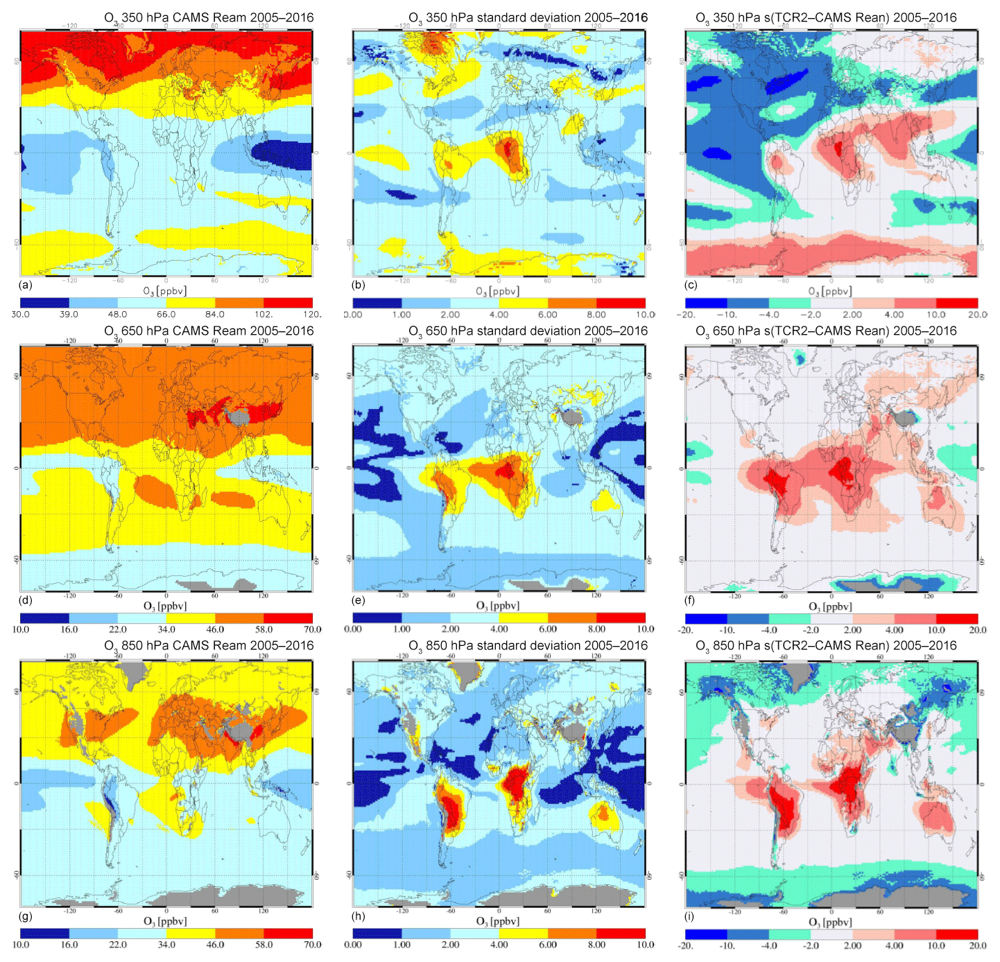
Figure 14 (a, d, g) Multiannual mean O₃ at 350, 650, and 850 hPa for the CAMS Reanalysis at 650 hPa over 2005–2016. (b, e, h) SD in the multiannual means for the four reanalyses. (c, f, i) Absolute difference between TCR-2 and CAMS Reanalysis (all in ppb).

Figure 15 Area-normalized frequency distributions of multiannual (2005–2016) mean O₃ mixing ratios at 850 (a), 650 (b), and 350 hPa (c) for the four reanalyses.

6 Evaluation of surface ozone in 2006

To assess the ability of reanalyses to cope with local situations, and specific meteorological conditions, we analysed their performance over Europe in 2006, with a focus on the ability to capture the diurnal and synoptic variabilities during the heatwave event that affected large parts of Europe during July 2006 (Struzewska and Kaminski, 2008). Here we use the ground-based observations from the EMEP network. For this evaluation, we note that these large-scale models do not represent local orography. Therefore, we select the appropriate model level depending on its pressure level, which is representative of mean pressure at the observation site (Flemming et al., 2009). Figure 10 presents the evaluation at two EMEP stations in Great Britain, during July 2006, illustrating the general performance of the reanalyses for this situation. The Lullington Heath station (50.8^∘ N, 0.2^∘ E; 120 $\mathrm{m}\mathrm{a}.\mathrm{s}.\mathrm{l}.$) is located in a nature reserve area, near the coast south of London. Great Dun Fell observatory (54.7^∘ N, 2.4^∘ W; 847 $\mathrm{m}\mathrm{a}.\mathrm{s}.\mathrm{l}.$) is located on a mountain summit, approximately 15 km north of Manchester. Both stations show enhanced levels of ozone in the first part of July, as well as during 16–20 July. In contrast to Great Dun Fell, Lullington Heath shows a pronounced diurnal cycle. For this evaluation, the reanalyses are sampled at different model levels (see figure caption). Note that the TCR reanalyses have fewer model levels towards the surface than the CAMS reanalyses. All reanalyses capture both the diurnal and synoptic variabilities with a significant improvement in TCR-2 compared to TCR-1, while the CAMS reanalyses are more alike. Particularly for Lullington Heath, the CAMS reanalyses and TCR-2 show remarkably small biases (MB<3.6 ppb). Also at Great Dun Fell the synoptic variability is generally well captured, particularly for the CAMS reanalyses and TCR-2.

A more quantitative assessment of the ability of the reanalyses to capture the ozone variability is presented in Figs. 11 and 12, which show a graphical presentation of the temporal correlation coefficient at EMEP stations for December–January–February (DJF) and June–July–August (JJA) 2006, computed by interpolating the reanalyses and observational results onto a common 3-hourly time frequency.

In the DJF period, regionally averaged correlation coefficients range from 0.45 (TCR-1) to 0.58 (CAMS-iRean). Comparatively high correlations were found over western Europe (particularly over the southern part of Britain), with R>0.8 for the CAMS reanalyses and R>0.6 for TCR. The lower correlations over the regions in the TCR reanalyses could be associated with its coarser model resolution.

For the summer period (JJA, Fig. 12), temporal correlations are overall higher than in the winter period, most markedly by better correlation statistics over south-western, eastern, and northern Europe. This is due to the more pronounced diurnal cycle during summer and results in generally consistent correlation over any of the stations across the European domain. The average values for R range between 0.61 (TCR-1) and 0.68 (CAMS-iRean). Only stations sampling ozone around the Mediterranean are consistently poorly captured, with R<0.5.

Temporal correlations for the March–April–May (MAM) and September–October–November (SON) seasons are in between those for DJF and JJA. The CAMS-Rean correlations are on average lower by ∼0.02 than those of CAMS-iRean, while TCR-2 has systematically improved by 0.02–0.05 over TCR-1.

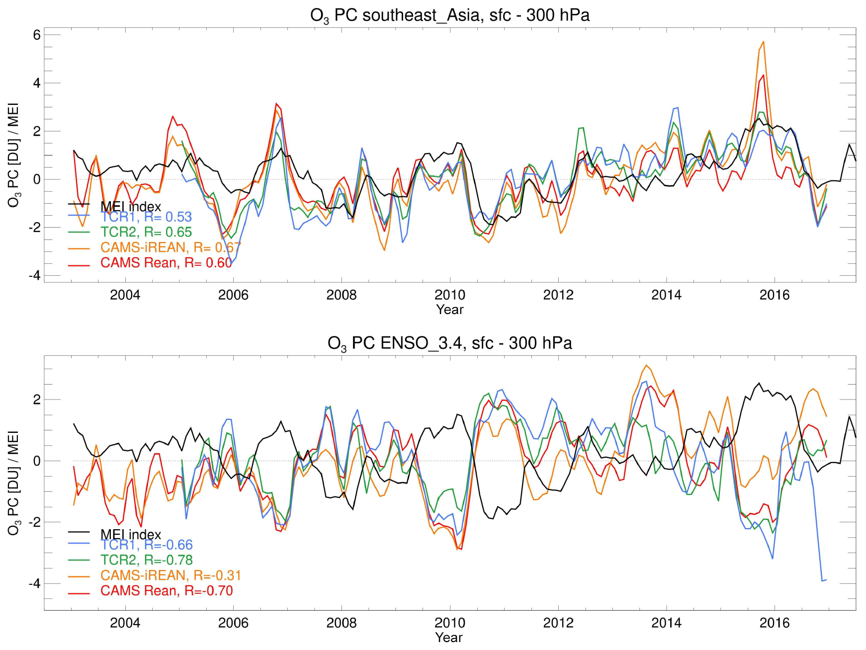
Figure 16 De-seasonalized anomalies in O₃ partial columns (surface to 300 hPa) in the four reanalyses, as compared to the MEI for two regions: Southeast Asia (10^∘ S–20^∘ N, 90–120^∘ E) and ENSO3.4 over the eastern Pacific ( 5^∘ S–5^∘ N, 120–170^∘ W). A 2-month smoothing has been applied to the reanalysis data (as for the MEI). Temporal correlations with respect to the MEI index are given in the legends. Correlations are calculated on monthly data for the 2005–2016 time period.

A closer look at the diurnal cycle for different seasons and regions over Europe is given in Fig. 13. In this figure the seasonal mean reanalysis biases have been subtracted in order to assess their ability to capture the diurnal cycle only. All reanalyses generally capture the diurnal variability and its variation across latitude region and season. For instance, all reanalyses show little diurnal variability for northern European stations during DJF, although the CAMS-based reanalyses (and particularly CAMS-Rean) show enhanced night-time O₃, which is not in TCR nor in the observations. Except for isoprene, no diurnal cycle in O₃ precursor emissions has been adopted in the CAMS reanalyses, which contributes to biases in the diurnal cycle. Note, however, that CAMS-Rean shows a comparatively large mean bias of −8 ppb for these conditions (CAMS-iRean bias is −6 ppb).

The diurnal cycle is generally larger for CAMS-iRean than CAMS-Rean, showing overall better correspondence to the observations. Particularly over middle and southern Europe during DJF, the CAMS reanalyses show a larger diurnal cycle than those obtained with TCR, and also matching better to the observations. For MAM, differences between the reanalyses are rather small, while during JJA the TCR-2 and CAMS-iRean show largest diurnal cycle across Europe, best matching again to the observations.

In summary, all reanalyses capture the synoptic to diurnal variabilities, as illustrated by the assessment of the heatwave event in July 2006. Still there are considerable differences in performance, depending on the reanalysis, region, and season. While CAMS-iRean and CAMS-Rean perform mostly similar, for TCR-2 a considerable improvement was found compared to TCR-1. Overall better temporal correlations are obtained for the summer period compared to winter and also for western Europe compared to the Mediterranean region. Further improvements can be obtained by a better description of surface processes, including emissions and deposition, together with higher spatial resolution modelling.

7 Global spatial and temporal consistency between reanalyses

Figure 14 shows the multiannual mean together with an evaluation of its multi-system standard deviation at different altitude levels. The standard deviation is computed from the multiannual means of the four reanalyses, and it provides a quantification of general agreement between reanalyses. The standard deviation at 850 and 650 hPa is relatively large over South America, central Africa, and Northern Australia, with values exceeding 6 ppb in the lower and middle troposphere. Normalized to local mean O₃ from the CAMS Reanalysis, the standard deviation values at 850 hPa reach 20 % over Australia and up to 50 % over South America and central Africa. At 650 hPa these maximum ratios decrease to approx. 10 % (Australia) and 20 % (South America and central Africa). These results suggest that the representation of biomass-burning emissions and its impacts on ozone production are largely different among the systems. Also large uncertainties in biogenic emissions likely contribute. In TCR, the optimization of NO_x emissions can have strong impacts on the lower and middle tropospheric ozone in contrast to the CAMS configuration which applies prescribed anthropogenic and biogenic emissions, combined with the daily-varying biomass-burning emissions. In addition, different representations of convective transport over the continents can lead to diversity in the vertical profile of ozone among the systems.

At 350 hPa, the multi-system standard deviation is large over central Africa, South America, and over the Arctic and Antarctic regions, which could reflect different representations of deep convection along with biomass-burning emissions at low latitudes and polar vortex, stratospheric ozone intrusions and chemistry treatment at high latitudes among the systems.

The absolute differences between the two most recent reanalyses, TCR-2 and CAMS-Rean, are also shown. Apart from the regions mentioned above, differences are significant around Alaska and Siberia, i.e. regions with tropospheric ozone influenced by biomass-burning events and where observational constraints at such high latitudes are more limited. Such larger discrepancies once again highlight the importance of the forecast model performance in the reanalysis system as discussed in Miyazaki et al. (2020), especially when direct observational constraints on tropospheric ozone are insufficient.

An evaluation of the consistency across the four reanalyses to describe the seasonal cycle of tropospheric ozone columns, and its interannual variability, is given in Fig. S6. From this, the difference in zonal mean partial columns (surface to 300 hPa) in the tropics is quantified: TCR-2 is on average higher than CAMS-Rean by 0.7 DU (2005) up to 1.8 DU (2016), corresponding to approx. 3 % to 8 % of the annual mean column in this region.

Frequency distributions of the multiannual mean ozone concentrations in the four reanalyses at three altitude levels are given in Fig. 15, and they summarize the general differences discussed above. In the lower and mid-troposphere the CAMS reanalyses show a larger frequency of O₃ values below 30 ppb (850 hPa) and 45 ppb (650 hPa) compared to TCR-1 in particular but also to TCR-2. This is associated with lower ozone in the CAMS reanalyses over the tropical regions. At 350 hPa the CAMS reanalyses and TCR-2 agree reasonably in their frequency distribution, with CAMS-iRean showing the largest frequency of relatively low (35–55 ppb) O₃ values, and instead TCR-1 shows a larger frequency of values in the range 70–100 ppb compared to the other reanalyses. This is associated with a positive reanalysis bias in this altitude range (see also Table 7). A corresponding evaluation of the frequency distributions, but sampled at individual ozone-sonde observations during the 2005–2016 period, is given in Fig. S7. Because of the different sampling approach, the shape of the frequency distributions is different than was seen in Fig. 15. Evaluation of the sum in absolute differences d between analysed and observed frequency distributions indicates that at 850 hPa the performance between the four reanalyses is very similar (d between 0.17 and 0.19), while at 650 hPa CAMS-Rean is superior (d=0.13). CAMS-iRean shows an underestimate of the frequency of high ozone values (larger than ∼55 ppbv) at 850 and 650 hPa, explaining the worst performance at 650 hPa (d=0.20). At 350 hPa the differences in performance between reanalyses are largest, with best correspondence to observations for CAMS-iRean (d=0.11) and worst for TCR-1 (d=0.43).

De-seasonalized anomalies in monthly-mean ozone tropospheric columns (surface to 300 hPa) have been computed over various regions by subtracting the reanalysis-specific mean seasonal cycle based on the 2005–2016 time series. Figure 16 presents the reanalysis anomalies together with the Multivariate ENSO Index (MEI) (Wolter and Timlin, 1998) for two regions. Tropical tropospheric ozone variations during El Niño conditions are in part associated with enhanced fire emissions, and corresponding ozone production, over Indonesia, together with suppressed convection (Inness et al., 2015), while the anti-correlation over the eastern Pacific is related to enhanced convection (Ziemke and Chandra, 2003). We find a significant correlation with R ranging between 0.6 (CAMS-Rean) and 0.65 (TCR-2) for the Southeast Asia region. A strong anti-correlation for the eastern Pacific region is found with R between −0.70 (CAMS-Rean) and −0.78 (TCR-2). The CAMS-iRean shows a lower correlation for this region, possibly associated with the jump in offset around the beginning of 2013, whose magnitude is significant in comparison to the signal.

An assessment of the consistency between all reanalyses to describe the de-seasonalized anomalies in various regions is given in Fig. S8 and Table S1 in the Supplement, i.e. in terms of the correlations in their anomalies. Specifically, the correlations between CAMS-Rean and TCR-2 over the Arctic and the eastern US are R=0.60 and R=0.63, respectively, giving some confidence to the robustness of this IAV signal in these reanalyses. For various other regions, correlations are R=0.52 (eastern Asia), R=0.42 (Europe), and R=0.33 (Antarctica). Also, when averaged over the full tropical zonal band, the correlation decreases to R=0.33, i.e. much smaller than correlations between CAMS-Rean and TCR-2 for the subregions Southeast Asia (R=0.82) and ENSO_3.4 (R=0.78). This implies that many of the IAV signals in the reanalyses should be considered with care.

8 Conclusions and discussion

Four tropospheric ozone reanalyses have been compared in this paper, namely CAMS-iRean, CAMS-Rean, TCR-1, and TCR-2. A range of independent observations was used to validate the quality of the chemical reanalyses at various spatial and temporal scales. These reanalyses aim to capture individual large-scale events, such as heatwaves or wildfires, and at the same time aim to provide a globally consistent climatology of present-day composition. This implies stringent requirements on their temporal consistency. The changes in the observing system, often combined with their limited sensitivity to tropospheric profiles and in particular the boundary layer, imply a significant dependency on the global chemistry model, its transport scheme, and its emissions, and this makes the generation of any long-term chemical reanalysis challenging. This gives rise to a detailed evaluation of the capability of the current reanalyses of tropospheric ozone, as presented here.

Consistent with Inness et al. (2019), our evaluation also shows substantial improvement of CAMS-Rean over CAMS-iRean in the free troposphere, as quantified by lower mean biases and standard deviations, higher correlations to ozone-sonde observations, and better temporal consistency in multiannual time series of tropospheric ozone columns. For instance, averaged over the NH midlatitude region, the mean bias in tropospheric ozone columns (surface to 300 hPa) is −0.3 DU (corresponding to approx. 1 % of observed tropospheric column) for CAMS-Rean, which was 0.8 DU (3 %) in CAMS-iRean.

At the surface the CAMS-Rean has generally improved with respect to CAMS-iRean, which are assessed through evaluations of monthly-mean surface concentrations against TOAR observations. Nevertheless, similar performances of both CAMS reanalyses were seen for hourly to sub-seasonal variabilities, as assessed with EMEP observations over Europe for the year 2006. The improved performance in the free troposphere can be attributed to a mixture of various upgrades, including revisions in the chemical data assimilation configuration, the chemistry mechanism, meteorological driver, model resolution, and biogenic emissions.

Significant changes in the quality of the ozone reanalyses for different years have been attributed to changes over time in the observing system. Both CAMS reanalyses suffered from the use of relatively poor SCIAMACHY and MIPAS data products before 2005, which improved afterwards. Also, in 2013 CAMS-iRean was affected by a switch of MLS version 2 to version 3.4. In both CAMS reanalyses a change to the vertical resolution of the assimilated SBUV/2 data during 2013 had a negative impact on the consistency of multiannual tropospheric ozone time series, particularly in polar regions. Inness et al. (2019) had noticed such a change in performance, but they had not yet identified the responsible observational dataset.

Compared with TCR-1, TCR-2 shows better agreements with independent observations throughout the troposphere, including at the surface. Similar to the CAMS reanalyses, for the NH mid-latitudes, the mean bias in tropospheric columns against ozone-sondes improved from 1.8 DU (7 %) in TCR-1 to 0.8 DU (3 %) in TCR-2. The improvements can be attributed to the use of more recent satellite retrievals and to an improved model performance, mainly associated with the increased model resolution. In spite of the good agreement with ozone-sonde measurements in the free troposphere, the surface ozone reanalysis exhibits large, positive biases over Europe and the United States. Also, the lack of the TES measurements led to a change in the reanalysis performance after 2010 for many regions in the lower and middle troposphere. Changes in the NO₂ observing system, including the OMI row anomaly after December 2009 and the limited temporal coverage of SCIAMACHY and GOME-2, are also considered to affect long-term consistency. The data assimilation diagnostics indicate the need for additional observational constraints, possibly combined with stronger inflation of the forecast error covariance to improve the long-term reanalysis performance and to measure the actual analysis uncertainty.

Whereas free-tropospheric ozone reanalyses agree well with independent observations, towards the surface larger biases have been found for many parts over the globe. A large spread at high latitudes could also be associated with the limited constraints from (tropospheric) ozone measurements. In these conditions the reanalyses depend more on the model performance and their emissions. Recently developed retrievals with high sensitivity to the lower troposphere (e.g. Deeter et al., 2013; Fu et al., 2018; Cuesta et al., 2018) would be helpful in improving the analysis of the lower troposphere. Furthermore, in future studies the analysis ensemble spread from EnKF can be regarded as uncertainty information about the analysis mean fields, indicating the need for additional observational constraints. Likewise, in the 4D-Var system the contributions from individual retrieval products can be tested.

We have demonstrated that the recent chemical reanalyses of CAMS-Rean and TCR-2 agree well with each other and with the independent observations in the majority of cases. This highlights the usefulness of the current chemical reanalyses in a variety of studies. For instance, the well-characterized, small mean bias in tropospheric columns in these reanalyses suggest that they can be used to provide a climatology of present-day tropospheric ozone. This may serve as a reference for the present-day contribution of tropospheric ozone to the radiation budget, or may provide a climatology for a priori ozone profiles as required for satellite retrieval products (e.g. Fu et al., 2018). The ability of the CAMS Reanalysis to capture the variability of (near-)surface ozone on multiple timescales, and for many regions over the globe, indicates it is fit for use as boundary conditions for hindcasts of regional air quality models.

Meanwhile, our intercomparisons suggest that the model configuration can still explain differences in the ozone reanalyses. For instance, differences in the representation of convective transport over the continents and those in the precursor's emissions, as well as differences in the chemical scheme, lead to substantial differences in the vertical profile of ozone and ozone production, such as over central Africa and South America. Here the standard deviation in annual mean ozone at 850 hPa reaches up to 50 % of the multi-reanalysis mean. The relatively coarse horizontal resolution in any of the global reanalysis configurations could also cause significant errors at urban sites. Therefore, both the data assimilation settings and the model performance are critical in improving the tropospheric ozone analysis and obtaining consistent data assimilation analysis, especially for the lower troposphere.

We have shown that discontinuities in the availability, coverage, and product version of the assimilated measurements affect the quality of any of the reanalyses, particularly in terms of temporal consistency. This is particularly important for assessing interannual variability. The influence of data discontinuities must be considered and where possible removed when studying interannual variability and trends using products from these reanalyses. To improve the temporal consistency in future reanalyses, a careful assessment of changes in the assimilation configuration, most prominently associated with ozone column and profile assimilation, is needed, including a detailed assessment of biases between various retrieval products.

The assimilation of multispecies data in both the CAMS and TCR configurations influences the representation of the entire chemical system, while the influence of persistent model errors in complex tropospheric chemistry continues to be a concern. Therefore, further improvements to long-term reanalyses of tropospheric ozone can be achieved by improving the observational constraints, together with a further optimization of model parameters, such as the chemical mechanism and emission, deposition, and mixing processes.