CE-DYNAM (v1): a spatially explicit process-based carbon erosion scheme for use in Earth system models

Soil erosion by rainfall and runoff is an important process behind the redistribution of soil organic carbon (SOC) over land, thereby impacting the exchange of carbon (C) between land, atmosphere, and rivers. However, the net role of soil erosion in the global C cycle is still unclear as it involves small-scale SOC removal, transport, and redeposition processes that can only be addressed over selected small regions with complex models and measurements. This leads to uncertainties in future projections of SOC stocks and complicates the evaluation of strategies to mitigate climate change through increased SOC sequestration.

In this study we present the parsimonious process-based Carbon Erosion DYNAMics model (CE-DYNAM) that links sediment dynamics resulting from water erosion with the C cycle along a cascade of hillslopes, floodplains, and rivers. The model simulates horizontal soil and C transfers triggered by erosion across landscapes and the resulting changes in land–atmosphere CO₂ fluxes at a resolution of about 8 km at the catchment scale. CE-DYNAM is the result of the coupling of a previously developed coarse-resolution sediment budget model and the ecosystem C cycle and erosion removal model derived from the Organising Carbon and Hydrology In Dynamic Ecosystems (ORCHIDEE) land surface model. CE-DYNAM is driven by spatially explicit historical land use change, climate forcing, and global atmospheric CO₂ concentrations, affecting ecosystem productivity, erosion rates, and residence times of sediment and C in deposition sites. The main features of CE-DYNAM are (1) the spatially explicit simulation of sediment and C fluxes linking hillslopes and floodplains, (2) the relatively low number of parameters that allow for running the model at large spatial scales and over long timescales, and (3) its compatibility with global land surface models, thereby providing opportunities to study the effect of soil erosion under global changes.

We present the model structure, concepts, limitations, and evaluation at the scale of the Rhine catchment for the period 1850–2005 CE (Common Era). Model results are validated against independent estimates of gross and net soil and C erosion rates and the spatial variability of SOC stocks from high-resolution modeling studies and observational datasets. We show that despite local differences, the resulting soil and C erosion rates, as well as SOC stocks from CE-DYNAM, are comparable to high-resolution estimates and observations at subbasin level.

We find that soil erosion mobilized around 66±28 Tg (10¹² g) of C under changing climate and land use over the non-Alpine region of the Rhine catchment over the entire period, assuming that the erosion loop of the C cycle was nearly steady state by 1850. This caused a net C sink equal to 2.1 %–2.7 % of the net primary productivity of the non-Alpine region over 1850–2005 CE. This sink is a result of the dynamic replacement of C on eroding sites that increases in this period due to rising atmospheric CO₂ concentrations enhancing the litter C input to the soil from primary production.

1 Introduction

Soils contain more carbon (C) than the atmosphere and living biomass together. Relatively small disturbances (anthropogenic or natural) to soil C pools over large areas could add up to substantial C emissions (Ciais et al., 2013). With the removal of natural vegetation and the introduction of mechanized agriculture, humans have accelerated soil erosion rates. Over the last 2 to 3 decades, studies have shown that water erosion (soil erosion by rainfall and runoff) amplified by human activities has substantially impacted the terrestrial C budget (Doetterl et al., 2012; Lal, 2003; Lugato et al., 2018; Van Oost et al., 2007, 2012; Stallard, 1998; Wang et al., 2017; Tan et al., 2020; Chappell et al., 2016). However, the net effect of water erosion on the C cycle at the regional-to-global scale is still under debate. This leads to uncertainties in the future projections of the soil organic C (SOC) reservoir, and it complicates the evaluation of strategies to mitigate climate change by increased SOC sequestration.

The study of Stallard (1998) was one of the first to show that water erosion not only leads to additional C emissions but also sequesters C due to the photosynthetic replacement of SOC at eroding sites and the stabilization of SOC in deeper layers at burial sites. The study by Van Oost et al. (2007) was the first to confirm the importance of the sequestration of SOC by agricultural erosion at a global scale using isotope tracers. Wang et al. (2017) gathered data on SOC profiles from erosion and deposition sites around the world and confirmed that water erosion on agricultural land that started from the early-to-middle Holocene has caused a large net global land C sink. Other studies, however, argue that soil erosion is a net C source to the atmosphere due to increased SOC decomposition following soil aggregate breakdown during transport and at deposition sites (Lal, 2003; Lugato et al., 2018). Most studies modeling soil erosion and its net effect on SOC dynamics at the global scale, however, do not account for the full range of complex effects of climate change, CO₂ -driven increase in productivity and potentially soil C inputs, harvest of biomass, land use change, and changes in cropland management (Borrelli et al., 2018; Doetterl et al., 2012; Chappell et al., 2016; Lugato et al., 2018; Van Oost et al., 2007; Wang et al., 2017). In addition, models used at large spatial scales mainly focus on hillslopes and removal processes and neglect floodplain sediment and SOC dynamics (Borrelli et al., 2018; Chappell et al., 2016; Lugato et al., 2018; Van Oost et al., 2007; Tan et al., 2020). This can lead to substantial biases in the assessment of net effects of SOC erosion at the catchment scale as floodplains can store substantial amounts of sediment and C (Berhe et al., 2007; Hoffmann et al., 2013a, b). Studies addressing long-term large-scale sediment yield from hillslopes and floodplains, such as Pelletier (2012), do not explicitly account for the redistribution of sediment and SOC over land.

Furthermore, soil erosion is one of the main contributors to particulate organic carbon (POC) fluxes in rivers and C export to the coastal ocean. The riverine POC fluxes are usually much smaller than the SOC erosion fluxes, due to decomposition and burial in floodplains and in benthic sediments, while POC losses occur in the river network (Tan et al., 2017; Galy et al., 2015). Therefore, uncertainties in large-scale SOC erosion rates over land will lead to even larger uncertainties in lateral C fluxes between land and ocean for past and future scenarios estimated by global empirical models on riverine C export (Ludwig and Probst, 1998; Mayorga et al., 2010).

To address these knowledge gaps, we present a parsimonious process-based Carbon Erosion DYNAMics model (CE-DYNAM), which integrates sediment dynamics resulting from water erosion with the SOC dynamics at the regional scale. The SOC dynamics are calculated consistently with drivers of land use change, CO₂, and climate change by a process-based global land surface model (LSM), with a simplified reconstruction of the last century increase of crop productivity. This modeling approach consists of a global sediment budget model coupled to the SOC removal, input, and decomposition processes diagnosed from the ORCHIDEE global LSM in an offline setting (Naipal et al., 2018). The main aim of our study is to quantify the horizontal transport of sediment and C along the continuum of hillslopes and floodplains and at the same time analyze its impacts on the land–atmosphere C exchange. We validate the new model with regional observations and high-resolution modeling results of the Rhine catchment. It should be noted here that the structure of CE-DYNAM is designed in a way that the model can be adapted easily to other large catchments after calibrating the model parameters to the specific environmental conditions in those catchments. We also discuss the model uncertainties and the sensitivity of the model to changes in key model parameters and assumptions made. In the next sections we give a detailed overview of the CE-DYNAM model structure; the coupling of erosion, deposition, and transport with the coarse-resolution SOC dynamics of ORCHIDEE; model application and validation for the non-Alpine region of the Rhine catchment; and its potential and limitations.

2 Methods

2.1 General model description

CE-DYNAM version 1 (v1) is the result of coupling a large-scale erosion and sediment budget model (Naipal et al., 2016) with the SOC scheme of the ORCHIDEE LSM (Krinner et al., 2005). The most important features of the model are (1) the spatially explicit simulation of lateral sediment and C transport fluxes over land, linking hillslopes and floodplains; (2) the consistent simulation of vertical C fluxes coupled with horizontal transport; (3) the low number of parameters compared to other C erosion models that operate at a high spatial resolution (Lugato et al., 2018; Billings et al., 2019), which allows for running the model at large spatial scales and over long timescales up to several thousands of years; (4) the generic input fields for application to any region or catchment; and (5) the compatibility with the modeling structure of LSMs.

In the ORCHIDEE LSM, terrestrial C is represented by eight biomass pools: four litter pools and three SOC pools. Each of the pools varies in space, time, and over the 12 plant functional types (PFTs). An extra PFT is used to represent bare soil. Anthropogenic and natural disturbances (as a result of climatic changes) to the C pools include fire, crop harvest, changes to the gross primary productivity (GPP), litterfall, and autotrophic and heterotrophic respiration (Krinner et al., 2005; Guimberteau et al., 2018). The C-cycle processes are represented by a C emulator that reproduces for each PFT all C pools and fluxes between the pools exactly as in ORCHIDEE in the absence of erosion. A net land use change scheme is included in the emulator with mass-conservative bookkeeping of SOC and C input when a PFT is changed into another PFT from anthropogenic land use change (Naipal et al., 2018). The sediment budget model has been added in the emulator to simulate large-scale long-term soil and SOC redistribution by water erosion using coarse-resolution precipitation, land-cover, and leaf area index (LAI) data from Earth system models (Naipal et al., 2015, 2016). The C emulator including erosion removal was developed by Naipal et al. (2018) to reproduce the SOC vertical profile, removal of soil and SOC, and compensatory SOC storage from litter input. As soil erosion is assumed to not change soil and hydraulic parameters but only the SOC dynamics, the emulator allows for substituting of the ORCHIDEE model and performing simulations on timescales of millennia with a daily time step and a spatial resolution of 5 arcmin ($\sim \mathrm{8}\mathrm{km}\times \mathrm{8}$ km), which would be a very computationally expensive or nearly impossible with the full LSM. The concept and all equations of the emulator are described in Naipal et al. (2018). The following subsections describe the different components of CE-DYNAM that couple the C and soil removal scheme (Naipal et al., 2018) with the horizontal transport and burial of eroded soil and C (Naipal et al., 2016).

Table 1 Model input datasets.

2.2 The soil erosion scheme

The potential gross soil erosion rates are calculated by the Adjusted Revised Universal Soil Loss Equation (Adj. RUSLE) model (Naipal et al., 2015), which is based on the Revised Universal Soil Loss Equation (RUSLE) (Renard et al., 1997) and is part of the sediment budget model (Naipal et al., 2016) (Fig. 1). In the Adj. RUSLE the yearly-average soil erosion rate is a product of rainfall erosivity (R), slope steepness (S), land cover and management (Cm), and soil erodibility (K):

$$\begin{array}{}\text{(1)}& E=S\times R\times K\times \mathrm{Cm}.\end{array}$$

Note that the original RUSLE model further includes a slope-length factor (L), which gives the length of a field in the direction of steepest descent, and a support practice factor (P), which accounts for management practices to mitigate soil erosion. These two factors have been excluded here, because their quantification still includes many uncertainties and is not practical for applications at regional to global scales. These factors are largely affected by local artificial structures (such as field size) and management practices, which are difficult to assess for the present day and whose changes over the past are even more uncertain. In addition, we focus in this study on the potential effect of soil erosion on the C budget without erosion-control (EC) practices.

Figure 1 A conceptual diagram of CE-DYNAM. The red arrows represent the C fluxes between the C pools and reservoirs, while the black arrows represent the links between the erosion processes (removal, deposition, and transport).

Naipal et al. (2015) have developed a methodology to derive the S and R factors from 5 arcmin resolution (5 arcmin×5 arcmin raster) data on elevation and precipitation, while at the same time preserving the high-resolution spatial variability in slope and temporal variability in erosivity. In the rest of the paper we will refer to X km (or arcmin) by X km (or arcmin) raster cells always with X km (or arcmin) resolution. Despite the comparatively coarse resolution of the erosion model, the so-derived R factor was shown to compare well with the corresponding high-resolution product published by Panagos et al. (2017). In the study by Naipal et al. (2016), where the soil erosion model was applied for the last millennium, the change in climate was taken into account in the calculation of the R factor. For this study, we assume that the climate zones as defined by the Köppen–Geiger climate classification have not changed drastically since 1850 CE.

2.3 The sediment deposition and transport scheme

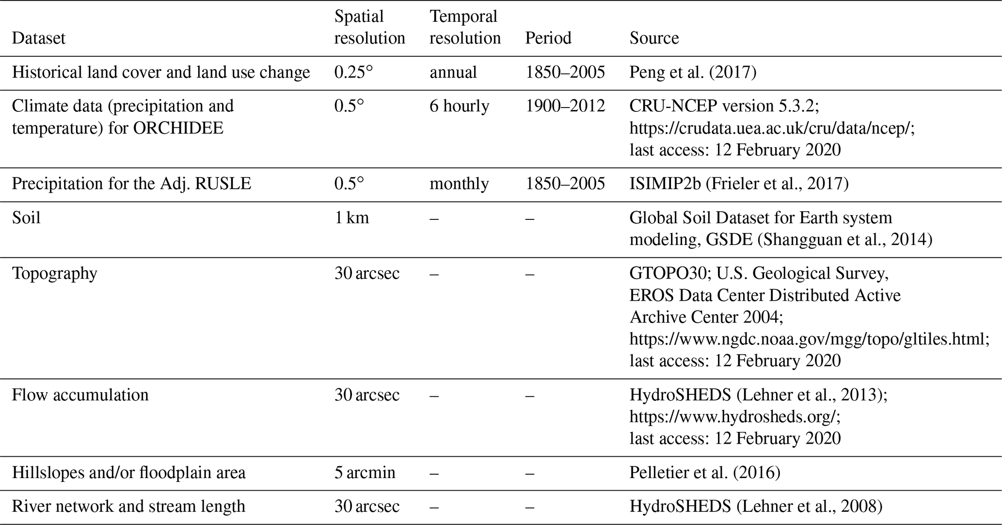
The sediment deposition and transport scheme is adapted from the sediment budget model described by Naipal et al. (2016), which was calibrated and validated for the Rhine catchment (Figs. 1, 2). In the sediment budget model rivers and streams are not explicitly simulated. Instead, each grid cell contains a floodplain fraction to ensure sediment transport between the grid cells. (Transport from one grid cell to another can only follow the connectivity of floodplains.) It should be noted that global soil databases do not identify floodplain soil as a separate soil class, although national soil databases might. Because we aim to present a carbon erosion model that should also be applicable for other similar catchments, we followed a two-step methodology to derive floodplains in the Rhine catchment. For this purpose, we used hydrological parameters and existing data on hillslopes and valleys. First, grid cells were identified that consisted entirely of floodplains. For this, we used the gridded global dataset of soil at 5 arcmin resolution, with intact regolith and sedimentary deposit thicknesses by Pelletier et al. (2016) (Table 1), and we identified lowlands and hillslopes based on soil thickness and depth to bedrock. The lowlands were classified as grid cells that contain only floodplains and no hillslopes. Second, we calculated the floodplain area fraction (A_fl) of a grid cell i, which has both hillslopes and floodplains as a function of stream length and width based on the methodology developed by Hoffmann et al. (2007) for the Rhine:

$$\begin{array}{}\text{(2)}& A_{\mathrm{fl}}\left(i\right)=L_{\mathrm{stream}}\left(i\right)\times W_{\mathrm{stream}}\left(i\right).\end{array}$$

Here, L_stream is the stream length derived from the HydroSHEDS database (Lehner and Grill, 2013) (Table 1).

$$\begin{array}{}\text{(3)}& W_{\mathrm{stream}}\left(i\right)=a\times A_{\mathrm{upstream}}^b\left(i\right)\end{array}$$

Here, A_upstream is the upstream catchment area, a is equal to 60.8, and b is equal to 0.3.

The parameters a and b have been derived using the scaling behavior of floodplain width as estimated from measurements on the Rhine (Hoffmann et al., 2007).

The sediment deposition on hillslopes (D_hs) and in floodplains (D_fl) is calculated as a function of the gross soil removal rates (E) according to Naipal et al. (2016) with the following equations:

$$\begin{array}{}\text{(4a)}& D_{\mathrm{fl}}\left(i\right)=f\left(i\right)\times E\left(i\right),\end{array}$$

$$\begin{array}{}\text{(4b)}& D_{\mathrm{hs}}\left(i\right)=\left(\mathrm{1}-f\left(i\right)\right)\times E\left(i\right),\end{array}$$

$$\begin{array}{}\text{(5)}& f\left(i\right)=a_f\times e^{\left(\frac{b_f\times \mathit{\theta }\left(i\right)}{{\mathit{\theta }}_{\max }}\right)}.\end{array}$$

Here, f is the floodplain deposition factor at 5 arcmin resolution that determines the fraction of eroded material transported and deposited in the floodplain fraction of a grid cell. a_f and b_f are constants that relate f to the average topographical slope (θ) of a grid cell depending on the type of land cover. θ_max is the maximum topographical slope of the entire Rhine catchment.

The parameters a_f and b_f are chosen in such a way that f varies between 0.2 and 0.5 for cropland, reflecting the decreased sediment connectivity between hillslopes and floodplains created by artificial structures such as ditches and hedges. For natural vegetation such as forests and natural grassland, a_f and b_f are chosen in a way that f varies between 0.5 and 0.8, assuming that in these landscapes hillslopes and floodplains are well connected. This assumption on the reduced sediment connectivity for agricultural landscapes is supported by several previous studies on the effect of erosion on sediment yield (Hoffmann et al., 2013a; De Moor and Verstraeten, 2008; Gumiere et al., 2011; Wang et al., 2015). These studies showed that anthropogenic activities on agricultural landscapes result in a trapping of eroded soil in colluvial deposition sites, reducing the sediment transport from hillslopes to floodplains. The model parameter f has been calibrated for the Rhine catchment by Naipal et al. (2016), where the ranges mentioned above are found to produce a ratio between hillslope and floodplain sediment storage that was comparable to observations. The studies by Wang et al. (2010, 2015) identified a range for the hillslope sediment delivery to be between 50 % and 80 %, which is similar to the range in the (1−f) factor in our model. In each case and within the defined boundaries, the slope gradient determines the final value of f. Eroded material that has not been deposited in the floodplains is assumed to be deposited at the foot of the hillslopes as colluvial sediment.

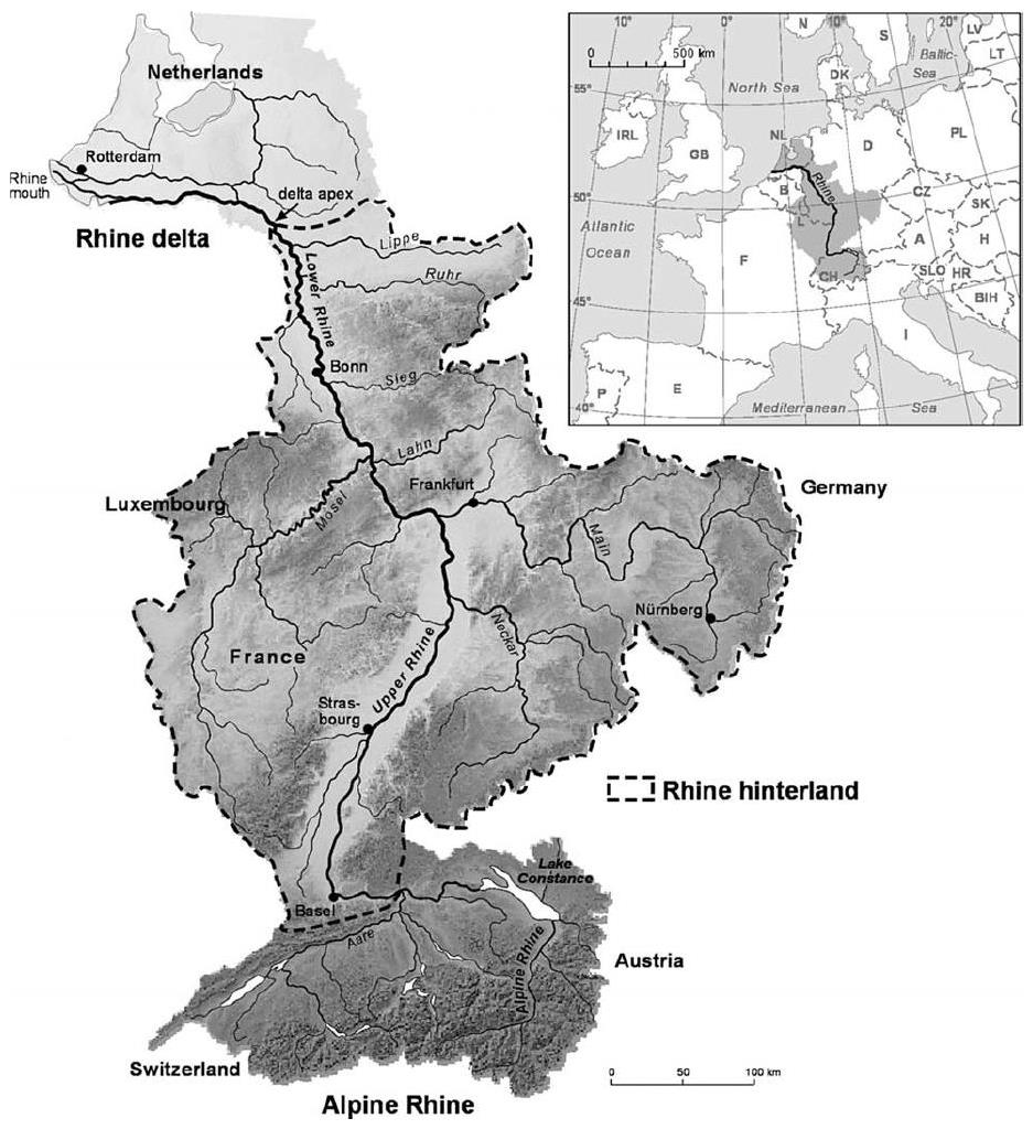
Figure 2 The Rhine catchment (Hoffmann et al., 2013a), where the gray shades represent elevation and the continuous black lines the main rivers.

The floodplain fractions of the grid cells are connected through a 5 arcmin resolution flow-routing network (Naipal et al., 2016), where the rivers and streams are indirectly included in the floodplain area but not explicitly simulated. By routing the sediment and C through the floodplain fractions of grid cells, we lump together the slow process of riverbank erosion by river dynamics (timescale is approximately equal to a few years to thousands of years), and the rather fast process of transport of eroded material by the rivers (timescale is approximately equal to days). The rate by which sediment and SOC leave the floodplain of a grid cell to go to the floodplain of an adjacent grid cell is determined by the sediment residence time. The sediment residence time (τ) is a function of the upstream contributing area (Flowacc):

$$\begin{array}{}\text{(6)}& \mathit{\tau }\left(i\right)=e^{\frac{\mathrm{Flowacc}\left(i\right)-a_{\mathit{\tau }}}{b_{\mathit{\tau }}}}.\end{array}$$

The study by Hoffmann et al. (2008) showed that the majority of floodplain sediments have a residence time that ranges between 0 and 2000 years, with a median of 50 years. The constants a_τ and b_τ are chosen in such a way that basin τ varies between the 5th and 95th percentiles of those observations, with a median for the whole catchment of 50 years. These constants are uniform for the whole basin, and need to be calibrated based on local data of sediment ages before CE-DYNAM can be applied to other catchments.

Floodplain SOC storage follows the same residence time as sediment on top of the actual decomposition rate of C in a grid cell of ORCHIDEE. The routing of sediment and C between the grid cells follows a multiple-flow routing scheme. In this scheme the flow coming from a certain grid cell is distributed across all lower-lying neighbors based on a weight (W, dimensionless) that is calculated as a function of the contour length (c):

$$\begin{array}{}\text{(7)}& W_{\left(i+k,j+l\right)}={\displaystyle \frac{{\mathit{\theta }}_{\left(i+k,j+l\right)}\times c_{\left(i+k,j+l\right)}}{\sum _{k,l=-\mathrm{1}}^{k,l=\mathrm{1}}\left[{\mathit{\theta }}_{\left(i+k,j+l\right)}\times c_{\left(i+k,j+l\right)}\right]}}.\end{array}$$

Here, c is 0.5 × grid size (m) in the cardinal direction and 0.354 × grid size (m) in the diagonal direction. (i,j) is the grid cell in consideration where i counts grid cells in the latitude direction and j in the longitude direction. i+k and j+l specify the neighboring grid cell where k and l can be either −1 0 or 1; θ is calculated as the division between the difference in elevation (h) given in meters and the grid cell size (d) (also in meters):

$$\begin{array}{}\text{(8)}& {\mathit{\theta }}_{\left(i+k,j+l\right)}={\displaystyle \frac{h_{\left(i,j\right)}-h_{\left(i+k,j+l\right)}}{d}}.\end{array}$$

The sediment and C routing is done continuously at a daily time step to preserve the numerical stability of the model. A more detailed explanation of the methods presented in this section can be found in the study by Naipal et al. (2016).

2.4 Litter dynamics

The four litter pools in the emulator are an belowground and an aboveground litter pool, each split into a metabolic and structural pool with different turnover rates as implemented in ORCHIDEE (Krinner et al., 2005). The belowground litter pools consist mostly of root residues. Both the biomass and litter pools have a loss flux due to fire as incorporated into ORCHIDEE by the SPITFIRE model of Thonicke et al. (2010). The litter that is not respired or burned is transferred to the SOC pools based on the CENTURY model (Parton et al., 1987), which was modified by Naipal et al. (2018) to include a vertical discretization scheme for SOC.

The vertical discretization scheme was introduced in the emulator to account for a declining C input and SOC respiration with depth, and it consists of 20 soil layers with 10 cm thickness each. The litter-to-soil fluxes from aboveground litter pools are all attributed to the top 10 cm of the soil profile. The litter-to-soil fluxes from belowground litter pools are distributed exponentially over the whole soil profile according to

$$\begin{array}{}\text{(9)}& I_{\mathrm{be}}\left(z\right)=I_{\mathrm{0}\mathrm{be}}\times e^{-r\times z}.\end{array}$$

Here, I_0be is the belowground litter input to the surface soil layer and r is the PFT-specific vertical root-density attenuation coefficient as used in ORCHIDEE. The sum of all layer-dependent litter-to-soil fractions is equal to the total litter to soil flux as calculated by ORCHIDEE. The vertical SOC profile is modified by erosion and the resulting deposition rates, which is discussed in detail in the following sections.

2.5 Crop harvest and yield

We adjusted the representation of crop harvest from ORCHIDEE by assuming a variable harvest index for C₃ plants that increases during the historical period as shown in the study of Hay (1995) for wheat and barley, which are also the main C₃ crops in the Rhine catchment. The harvest index is defined by the ratio of harvested grain biomass to aboveground dry matter production (Krinner et al., 2005). In this study the harvest index increases linearly between 0.26 and 0.46 (Naipal et al., 2018), which is consistent with the average values of Hay (1995).

Furthermore, we found that in certain cases the cropland net primary productivity (NPP) was too high during the entire period of 1850–2005, especially in the early part of the 20th century. This is because the cropland photosynthetic rates were adjusted in ORCHIDEE to give a cropland NPP representative of present-day values that are higher than for the low input agriculture of the early 20th century. To derive a more realistic NPP for wheat and barley in the Rhine catchment, we used the long-term crop yield data obtained from a dataset on 120 000 yield observations over the 20th century in northeast French departments (NUTS3 administrative division) (Schauberger et al., 2018). According to the yield data assembled by Schauberger et al. (2018), yields in northeast France (covering part of the Rhine catchment) for these crops increased fourfold during the last century. Note that crop residues like straw constituted a larger fraction of the total biomass in 1850 than in 2005, but those residues were likely collected and used for animal feed and housing fuel. We did not account for this harvest of residue in the simulation of SOC.

2.6 SOC dynamics without erosion

The change in the C content of the PFT-specific SOC pools in the emulator without soil erosion was described by Naipal et al. (2018) (Fig. 1) as follows:

$$\begin{array}{}\text{(10)}& \begin{array}{rl}{\displaystyle \frac{{\mathrm{dSOC}}_{\mathrm{a}}\left(t\right)}{\mathrm{d}t}}& ={\mathrm{lit}}_{\mathrm{a}}\left(t\right)+k_{\mathrm{pa}}\times {\mathrm{SOC}}_{\mathrm{p}}\left(t\right)+k_{\mathrm{sa}}\\ & \times {\mathrm{SOC}}_{\mathrm{s}}\left(t\right)-\left(k_{\mathrm{ap}}+k_{\mathrm{as}}+k_{\mathrm{0}\mathrm{a}}\right)\times {\mathrm{SOC}}_{\mathrm{a}}\left(t\right),\end{array}\end{array}$$

$$\begin{array}{}\text{(11)}& \begin{array}{rl}{\displaystyle \frac{{\mathrm{dSOC}}_{\mathrm{s}}\left(t\right)}{\mathrm{d}t}}& ={\mathrm{lit}}_{\mathrm{s}}\left(t\right)+k_{\mathrm{as}}\times {\mathrm{SOC}}_{\mathrm{a}}\left(t\right)\\ & -\left(k_{\mathrm{sa}}+k_{\mathrm{sp}}+k_{\mathrm{0}\mathrm{s}}\right)\times {\mathrm{SOC}}_{\mathrm{a}}\left(t\right),\end{array}\end{array}$$

$$\begin{array}{}\text{(12)}& \begin{array}{rl}{\displaystyle \frac{{\mathrm{dSOC}}_{\mathrm{p}}\left(t\right)}{\mathrm{d}t}}& =k_{\mathrm{ap}}\times {\mathrm{SOC}}_{\mathrm{a}}\left(t\right)+k_{\mathrm{sp}}\times {\mathrm{SOC}}_{\mathrm{s}}\left(t\right)\\ & -(k_{\mathrm{pa}}+k_{\mathrm{0}\mathrm{p}})\times {\mathrm{SOC}}_{\mathrm{p}}\left(t\right).\end{array}\end{array}$$

Here, SOC_a, SOC_s, and SOC_p (g C m⁻²) are the active, slow, and passive SOC, respectively. The distinction of these SOC pools, defined by their residence times, are based on the study by Parton et al. (1987). The active SOC pool has the lowest residence time (1–5 years) and the passive the highest (200–1500 years). lit_a and lit_s (g C m⁻² d⁻¹) are the daily litter input rates to the active and slow SOC pools, respectively; k_0a, k_0s, and k_0p (d⁻¹) are the respiration rates of the active, slow, and passive pools, respectively; k_as, k_ap, k_pa, k_sa, and k_sp are the coefficients determining the flux from the active to the slow pool, from the active to the passive pool, from the passive to the active pool, from the slow to the active pool, and from the slow to the passive pool, respectively.

The vertical C discretization scheme in the emulator assumes that the SOC respiration rates decrease exponentially with depth:

$$\begin{array}{}\text{(13)}& k_i\left(z\right)=k_{\mathrm{0}i}\left(z\right)\times e^{-\mathrm{re}\times z}.\end{array}$$

Here, k_i is the respiration rate at a soil depth z, and “re” (m⁻¹) is a coefficient representing the impact of external factors, such as decreasing oxygen availability with depth. k₀ is the respiration rate of the surface soil layer for a certain SOC pool i. The variable re is determined in such a way that the total soil respiration of a certain pool over the entire soil profile without erosion is similar to the output of the full ORCHIDEE model. A detailed description of how this is done can be found in the study by Naipal et al. (2018).

2.7 Net C erosion on hillslopes

In the model we assume that soil erosion takes place on hillslopes and not in the floodplains, due to the usually low topographical slope of floodplains. The factor (1−f) determines the fraction of the eroded soil that is deposited in the colluvial reservoirs (Fig. 1, Eq. 4b). Soil erosion always removes a fraction of the SOC stock in the upper soil layer depending on the erosion rate and bulk density of the soil. The next soil layer contains less C and therefore at the following time step less C will be eroded under the same erosion rate. In the model, the SOC-profile evolution is dynamically tracked and updated at a daily time step, which conforms with the method of Wang et al. (2015). First, a fraction of the C from each soil pool in proportion to the erosion rate is removed from the surface layer. Then, at the same erosion rate, SOC from the subsoil layer becomes the surface layer, maintaining the soil layer thickness in the vertical discretization scheme. Similarly, the SOC from the subsoil later also moves upward one layer. The removal of C by erosion triggers a compensatory C sink due to the reduction in SOC respiration on eroding land. This compensatory C sink and reduced C erosion over time will ultimately lead to an equilibrium state. The change in C content due to net erosion (the eroded sediment or C that leaves the hillslopes after deposition) of the PFT-specific pools for hillslopes can be represented by the following equations:

$$\begin{array}{}\text{(14)}& \begin{array}{rl}{\displaystyle \frac{{\mathrm{dSOC}}_{\mathrm{HSi}}\left(z,t\right)}{\mathrm{d}t}}& =k_{\mathrm{E}}\times {\mathrm{SOC}}_{\mathrm{HSi}}\left(z+\mathrm{1},t\right)-k_{\mathrm{E}}\\ & \times {\mathrm{SOC}}_{\mathrm{HSi}}\left(z,t\right),\end{array}\end{array}$$

where dSOC_HSi(z,t) is the change in hillslope SOC of a component pool i at a depth z and at time step t. The daily net erosion fraction, k_E (dimensionless), is calculated as the following:

$$\begin{array}{}\text{(15)}& k_{\mathrm{E}}={\displaystyle \frac{f\times \left(\frac{E}{\mathrm{365}}\right)}{\mathrm{BD}\times \mathrm{d}z}}\times \mathrm{EF},\end{array}$$

where E is the gross soil erosion rate (t ha⁻² yr⁻¹) (note “ha” represents hectare), f is the floodplain deposition factor, BD is the average bulk density of the soil profile (g cm⁻³), dz is the soil thickness (equal to 0.1 m), and EF is the C enrichment factor that is set to 1 by default. A model sensitivity analysis will be performed (see Sect. 4.3) with EF>1 to represent a higher C concentration in eroded soil compared to the original soil as a result of the selectivity of erosion.

Hillslope erosion without the deposition term has already been tested and applied at the global scale as part of the C removal model presented by Naipal et al. (2018).

2.8 C deposition and transport in floodplains

The SOC-profile dynamics of floodplains are controlled by (1) C input from the hillslopes, (2) C import by lateral transport from the floodplain fractions of upstream grid cells, and (3) C export to the floodplain fractions of downstream grid cells (Fig. 1). First, the net erosion flux from the surface layer of the hillslope fraction of the grid cell (k_E×SOC_HS at z=0) is incorporated into the surface layer of the floodplain. At the same deposition rate, the SOC of the surface layer of the floodplain is incorporated into the subsoil layer. Similarly, a fraction of the SOC of the subsoil layer is moved downward one layer. We will refer to this process as the “downward” moving of C in the soil layer profile. It should be noted that C selectivity during transport and deposition is not taken into account here, meaning that the C pools of the deposited material are the same as the eroded material from the topsoil of eroding areas. At the same time as deposition takes place a fraction of the C of the surface layer proportional to the sediment residence time (τ) is exported out of the catchment following the sediment routing scheme, resulting in the “upward” moving of the C from the subsoil layers. This process represents the river bank erosion and resulting POC export by the water network, although rivers and streams are not explicitly represented in the model. As we do not have information on the subgrid spatial distribution of land cover fractions, we first sum the exported C flux over all PFTs before assigning the flux proportionally to the land cover fractions of the receiving downstream-located grid cells. The C that is imported from the neighboring grid cells follows the same procedure as the deposition of eroded material, and this results in a downward moving of the C in the soil profile. The change in C content due to deposition and routing of the PFT-specific SOC pools for floodplains can be represented by the following equations:

$$\begin{array}{}\text{(16)}& \begin{array}{rl}{\displaystyle \frac{{\mathrm{dSOC}}_{\mathrm{FLi}}\left(z,t\right)}{\mathrm{d}t}}& =\left(\left(k_{\mathrm{D}}+k_{i_{\mathrm{out}}}\right)\times {\mathrm{SOC}}_{\mathrm{FLi}}\left(z-\mathrm{1},t\right)\right)\\ & +\left({\displaystyle \frac{\mathrm{1}}{\left(\mathit{\tau }\times \mathrm{365}\right)}}\times {\mathrm{SOC}}_{\mathrm{FLi}}\left(z+\mathrm{1},t\right)\right)\\ & -\left(\left(k_{\mathrm{D}}+{\displaystyle \frac{\mathrm{1}}{\left(\mathit{\tau }\times \mathrm{365}\right)}}+k_{i_{\mathrm{out}}}\right)\right.\\ & \left.\times {\mathrm{SOC}}_{\mathrm{FLi}}\left(z,t\right)\right),\text{for}z>\mathrm{0};\end{array}\end{array}$$

$$\begin{array}{}\text{(17)}& \begin{array}{rl}{\displaystyle \frac{{\mathrm{dSOC}}_{\mathrm{FLi}}\left(\mathrm{0},t\right)}{\mathrm{d}t}}& ={\sum }_{n=\mathrm{1}}^{n=\mathrm{9}}\left(k_{i_{\mathrm{out}}}\left(n\right)\times {\mathrm{SOC}}_{\mathrm{FLi}}\left(\mathrm{0},t\right)\left(n\right)\right)\\ & +\left(k_{\mathrm{E}}\times {\mathrm{SOC}}_{\mathrm{HSi}}\left(\mathrm{0},t\right)\right)\\ & +\left({\displaystyle \frac{\mathrm{1}}{\left(\mathit{\tau }\times \mathrm{365}\right)}}\times {\mathrm{SOC}}_{\mathrm{FLi}}\left(\mathrm{1},t\right)\right)\\ & -\left(\left(k_{\mathrm{D}}+{\displaystyle \frac{\mathrm{1}}{\left(\mathit{\tau }\times \mathrm{365}\right)}}+k_{i_{\mathrm{out}}}\right)\right.\\ & \left.\times {\mathrm{SOC}}_{\mathrm{FLi}}\left(\mathrm{0},t\right)\right),\text{for}z=\mathrm{0};\end{array}\end{array}$$

where n is the neighboring grid cell that flows into the current grid cell, dSOC_FLi (z,t) is the change in floodplain SOC of a component pool i at a depth z and at time step t, and SOC_HS is the hillslope SOC stock. k_D is the deposition rate and equal to

$$\begin{array}{}\text{(18)}& k_{\mathrm{D}}={\displaystyle \frac{k_{\mathrm{E}}\times {\mathrm{AREA}}_{\mathrm{HS}}}{{\mathrm{AREA}}_{\mathrm{FL}}}},\end{array}$$

where AREA_HS is the hillslope area and AREA_FL is the floodplain area (m²) of a grid cell. $k_{i_{\mathrm{out}}}$ is the import rate per C pool i from neighboring grid cells (dimensionless) and can be calculated as

$$\begin{array}{}\text{(19)}& k_{i_{\mathrm{out}}}={\displaystyle \frac{\sum _{n=\mathrm{1}}^{n=\mathrm{9}}(W\times \frac{\mathrm{1}}{\mathit{\tau }\times \mathrm{365}}\times {\mathrm{AREA}}_{\mathrm{FL}})\left(n\right)}{{\mathrm{AREA}}_{\mathrm{FL}}}},\end{array}$$

where W is the weight index of Eq. (7).

The first term of Eq. (16) represents the downward moving of the incoming C related to the C deposition flux from the hillslope fraction of the grid cell and the lateral C import flux from the floodplain fractions of upstream neighboring grid cells. The second term represents the upward moving of SOC related to the lateral C transfer to downstream neighboring grid cells. The third term of Eq. (16) represents the total C loss flux from the current soil layer z, which is a result of either the upward or downward moving of the C in the soil profile. The first term of Eq. (17) represents the incoming lateral C flux from the floodplains of the upstream neighboring grid cells. The second term represents the C deposition flux coming from the hillslope fraction of the grid cell. The third term represents the upward moving of the SOC from the subsoil layer to the topsoil layer as a result of sediment or C routing. The last term of Eq. (17) represents the total loss of C from the topsoil layer, of which part is distributed across the neighboring grid cells downstream ($\frac{\mathrm{1}}{\left(\mathit{\tau }\times \mathrm{365}\right)})$, and part is moved “downwards” in the soil profile as a result of C deposition (k_D) and the incoming lateral C from upstream grid cells ($k_{i_{\mathrm{out}}})$.

2.9 The land use change bookkeeping model

The land use change bookkeeping scheme includes the yearly changes in forest, grassland, and cropland areas in each grid cell as reconstructed by Peng et al. (2017) (Table 1). Peng et al. (2017) derived historical changes in PFT fractions based on the LUHv2 land use dataset (Hurtt et al., 2011), historical forest area data from Houghton (2003), and the present-day forest area from ESA CCI satellite land cover (European Space Agency, 2014). By using different transition rules and independent forest data to constrain the changes in crop and urban PFTs, they derived the most suitable historical PFT maps.

When land use change takes place, the litter and SOC pools of all shrinking PFTs are summed and allocated proportionally to the expanding PFTs, maintaining the mass balance. In this way the litter pools and SOC stocks get impacted by different input and respiration rates for each soil layer. When forest is reduced, three wood products with decay rates of 1, 10, and 100 years are formed and harvested. The biomass pools of other shrinking land cover types are transformed to litter and allocated to the expanding PFTs. More details on the land use scheme are described in the study by Naipal et al. (2018).

2.10 Study area

The model is tested for the Rhine catchment (Fig. 2), which has a total basin area of about 185 000 km² covering five different countries in central Europe. Its large size is beneficial for the application of a coarse-resolution model such as CE-DYNAM to study large-scale regional dynamics in the C cycle due to soil erosion. The Rhine catchment has a contrasting topography, with steep slopes larger than 20 % upstream in the Alps, and large, wide, and flat floodplains at the foot of the Alps, the Upper Rhine, and the Lower Rhine. The floodplains store large amounts of sediment and C that originate from eroding hillslopes upstream. These sediment storages provide the possibility to study the long-term effect of erosion on hillslope and floodplain dynamics. Furthermore, the Rhine catchment has been experiencing different stages of land use change over the Holocene, with land degradation dating back to more than 5500 years ago (Dotterweich, 2013). In contrast, during the last 2 decades there has been a general afforestation and soil erosion has been decreasing. These land use changes and changes in erosion make an interesting and important case to study the effect of anthropogenic activities on the C cycle in Europe.

In addition, the Rhine catchment has been the focus of many erosion studies providing observations on erosion and sediment dynamics that can be used for model validation (Asselman, 1999; Asselman et al., 2003; Erkens, 2009; Hoffmann et al., 2007, 2008, 2013a, b; Naipal et al., 2016). The global sediment budget model that forms the basis for the sediment dynamics scheme of CE-DYNAM has been validated and calibrated for the Rhine catchment with observations on sediment storage from Hoffmann et al. (2013a) and scaling relationships between sediment storage and basin area (Naipal et al., 2016). Hoffmann et al. (2008, 2013a) did an inventory of 41 hillslope and 36 floodplain sediment and SOC deposits related to soil erosion over the last 7500 years. The floodplain sediment observations consist mostly of organic material (gyttja, peat) and fine sediments (fine sand, loam, silt) in overbank deposits (Hoffmann et al., 2008). These fine sediments are a result of long-term soil erosion on the hillslopes. Hoffmann et al. (2013a) found that the sediment and SOC deposits were quantitatively related to the basin size according to certain scaling functions, where floodplain deposits increased in a nonlinear way with basin size, while the hillslope deposits showed a linear increase with basin size. We use these relationships to validate the spatial variability in SOC storage of floodplains and hillslopes simulated by CE-DYNAM. The scaling relationships have the form of a simple power law:

$$\begin{array}{}\text{(20)}& M=a\times {\left({\displaystyle \frac{A}{A_{\mathrm{ref}}}}\right)}^b,\end{array}$$

where M is the sediment storage or the SOC storage, a is the storage (Mt) related to an arbitrary chosen area A_ref, and b is the scaling exponent.

2.11 Input data and model simulations

To create the C emulator that forms the underlying C cycle of CE-DYNAM, we first ran the full ORCHIDEE model for the period 1850–2005 at a coarse resolution of 2.5^∘ latitude and 3.75^∘ longitude, and we output all C pools and fluxes. The pools and fluxes were then archived together and used to derive the turnover rates to build the emulator. The SOC scheme of the emulator that has been modified to account for soil erosion processes was made to run at a spatial resolution of 5 arcmin, similar to the original global sediment budget model. Then, we performed three main simulations with CE-DYNAM for the Rhine catchment. Simulation S0 is the baseline simulation or no-erosion simulation, where SOC dynamics are similar to the full ORCHIDEE model. Simulation S1 is the erosion-only simulation, where the hillslopes erode and all eroded C is respired to the atmosphere without reaching the colluvial and alluvial deposition sites. Simulation S2 is the simulation with full sediment dynamics, where hillslopes and floodplains are connected and can store or lose C. We ran the emulator for 3000 years at a daily time step with the initial climate and land cover of the period 1850–1860. To speed up the spin-up simulations we calculated the temporary equilibrium state of the floodplain SOC pools every 10 years analytically. At the end of the spin-up period the floodplain SOC pools were close to equilibrium, with a yearly change of less than 0.001 % of the total floodplain SOC stock. Afterwards, we performed the transient simulations for the period 1851–2005 at a daily time step with changing climate and land cover conditions, using the equilibrium SOC stocks as baseline. To ensure a faster performance of CE-DYNAM, we delineated the Rhine catchment into seven large subbasins and ran the model in parallel for each of the subbasins at a daily time step. After each year the subbasins exchanged the lateral C fluxes with each other.

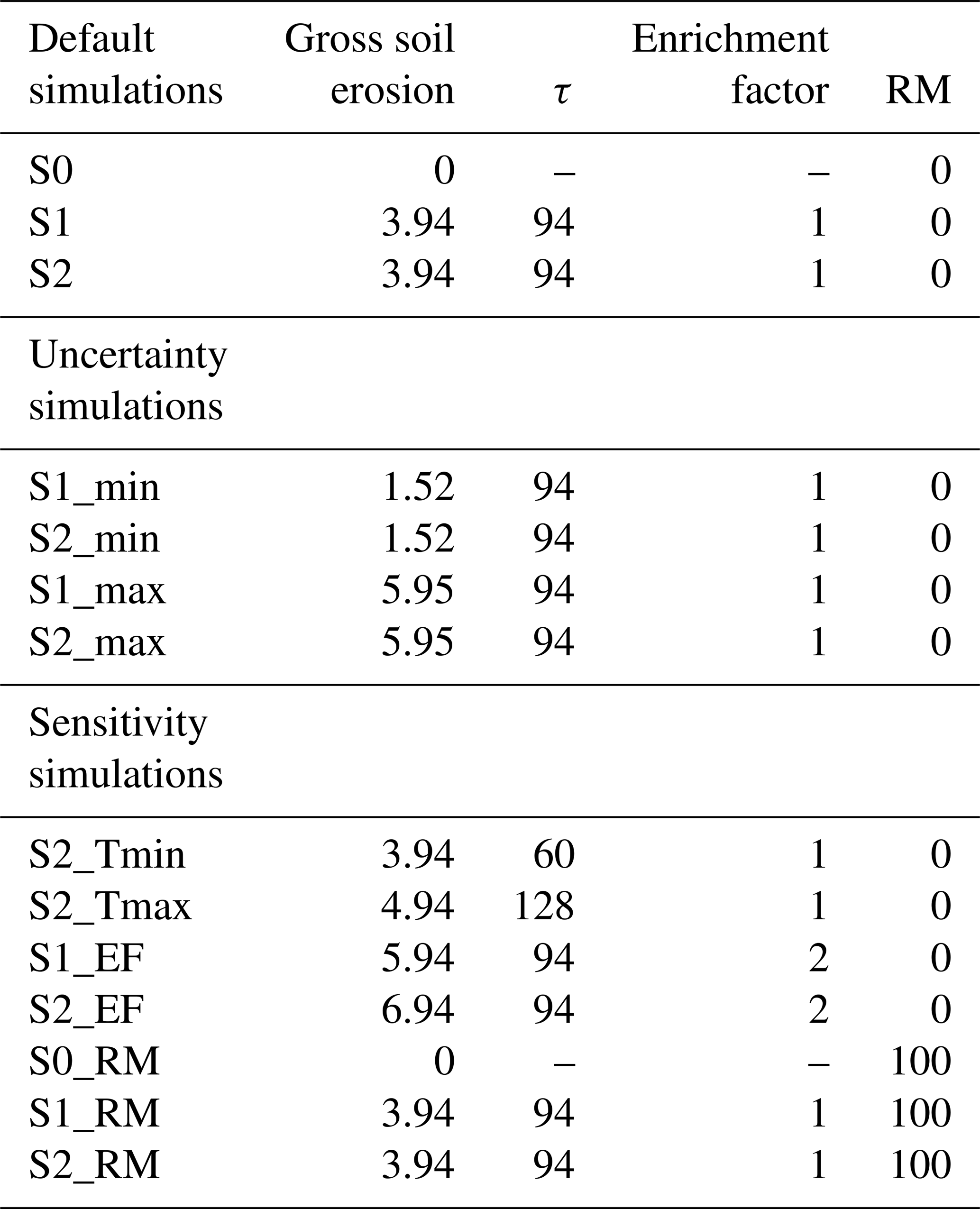
We also performed seven additional sensitivity simulations and four additional uncertainty simulations. Simulation S1_EF and S2_EF are performed to test the model assumption of C enrichment during erosion. Here, we changed the enrichment factor EF to 2, based on the study by Lugato et al. (2018). Simulations S2_Tmin and S2_Tmax are performed to test the rate of C transport between floodplains. Here we modified the mean sediment residence time for the Rhine catchment to a minimum of 60 years (50 % lower than the current value) and to a maximum of 128 years (50 % higher than the current value), respectively. However, we kept the maximum sediment residence time at 1500 years. Simulations S0_RM, S1_RM, and S2_RM are performed to test the model assumption on crop residue management, where we assumed that all aboveground crop litter is harvested.

For the uncertainty analysis, we performed simulations S1_min and S2_min based on a minimum soil erosion scenario and S1_max and S2_max based on a maximum soil erosion scenario. These soil erosion scenarios are derived from the uncertainty ranges in the rainfall erosivity and land cover factors of the erosion model. All the model simulations are summarized in Table 2.

Table 2 Model simulations, with changes to the basin average gross soil erosion rate (t ha⁻¹ yr⁻¹), the basin average sediment residence time τ (years), the enrichment factor, and the crop residue harvest intensity RM (%).

2.12 Validation methods and data

We performed a detailed model validation of the sediment and the C parts of the model according to the following steps: (1) validation of soil erosion rates using observational and high-resolution model estimates for Germany and Europe, (2) validation of C erosion rates using high-resolution model estimates for Europe from Lugato et al. (2018), (3) validation of the spatial variability of hillslope and floodplain C storage using observational results from Hoffmann et al. (2013a), and (4) validation of SOC stocks using observational data from a global soil database and a European land use survey.

The validation of the soil erosion module has been done before in the studies by Naipal et al. (2015, 2016). However, we do it again in this study due to different input datasets. In addition, the validation includes soil erosion data from new global soil erosion studies such as Borrelli et al. (2018) and Panagos et al. (2015). For the validation of gross soil erosion rates, we used the high-resolution model estimates of Panagos et al. (2015), who applied the RUSLE2015 model at a 100 m resolution at European scale for the year 2010. Similarly to the Adj.RUSLE, RUSLE2015 is also derived from the original RUSLE model. However, in contrast to our model, RUSLE2015 does include the erosion factors L and P. Furthermore, our model uses more coarsely resolved input datasets (Table 1), for which the equations for the R and S factors have been modified. Thus, even though both Adj.RUSLE and RUSLE2015 are derived from the same erosion model, the differences between the models are large, which justifies our model comparison. The extensive validation of the Adj.RUSLE model in this study and previous studies (Naipal et al., 2015, 2016, 2018) shows that despite its coarse resolution, it is applicable at large spatial scales.

Furthermore, we used independent high-resolution erosion estimates from the study by Cerdan et al. (2010), available at a 1 km resolution at European scale, which were based on an extensive database of measured erosion rates under natural rainfall in Europe. For the comparison, we aggregated the high-resolution model results of both datasets to the resolution of CE-DYNAM. We also used the potential soil erosion map of the Federal Institute for Geosciences and Natural Resources of Germany (Bug et al., 2014) for comparison. This map presents the yearly-average soil erosion rates at a 250 m resolution on agricultural land derived from a USLE-based approach (Universal Soil Loss Equation), with some modifications to the erosion factors and input data. Before validating our model results we aggregated these high-resolution erosion rates also to the coarser resolution of our model.

Validation of our net soil erosion rates is done based on the 100 m resolution net soil erosion rates derived with the WATEM/SEDEM model (Borrelli et al., 2018). WATEM/SEDEM simulates soil removal by water erosion based on the USLE approach, sediment transport, and deposition based on the transport capacity. The model has been extensively employed to estimate net fluxes of sediments across hillslopes at catchment and regional scales.

For the validation of C erosion rates, we used the high-resolution model results from Lugato et al. (2018), where they coupled the RUSLE2015 erosion model to the CENTURY biogeochemistry model. These model results were available at a resolution of 1 km, where each grid cell was composed of an erosion and deposition fraction. The C erosion rates provided by Lugato et al. (2018) were multiplied with the erosion fraction of a 1 km grid cell. Then, the C erosion rates were aggregated to the resolution of CE-DYNAM. Lugato et al. (2018) provided an enhanced and a reduced erosion-induced C sink uncertainty scenario, based on different assumptions for C enrichment, burial, and C mineralization during transport. In CE-DYNAM the C erosion rates from simulation S1 are multiplied with the hillslope area to get the total C erosion flux of a grid cell. As the study by Lugato et al. (2018) considers only agricultural areas, we considered only the crop fraction of a grid cell during the comparison. It should be noted that the SOC dynamics scheme of CE-DYNAM, which is derived from ORCHIDEE LSM, is also based on the CENTURY model. However, there are large differences between the CENTURY model used by Lugato et al. (2018) and the C dynamics scheme of ORCHIDEE used in this study. For example, in the CENTURY model the crop productivity is mediated by nitrogen availability, which is not the case in the ORCHIDEE version used for this study. The CENTURY model also includes some management practices such as crop rotations, which are not represented in ORCHIDEE. The CENTURY model runs at a much higher resolution and is calibrated for agricultural land, while ORCHIDEE also simulates forest, grasslands, and bare soil. In this way, the final SOC stocks derived with CE-DYNAM are also a result of erosion from other land cover types and land use changes. This is an important feature for land use change, which is not included in the CENTURY model. Furthermore, the ORCHIDEE LSM has been used in many global intercomparisons and extensively evaluated for C budgets (Müller et al., 2019; Todd-Brown et al., 2013). Finally, ORCHIDEE also includes the last century change in crop production calibrated against data (Guenet et al., 2018).

For the validation of the spatial variability of the SOC stocks of hillslopes and floodplains, we used the scaling relationships between basin area and SOC storage derived by Hoffmann et al. (2013a). The study by Naipal et al. (2016) found that the global sediment budget model is able to reproduce the scaling behavior of sediment storage. After analyzing the dependence of this scaling behavior, they argue that it is an emergent feature of the model and mainly dependent on the underlying topography. This indicates that the scaling features of floodplain and hillslope sediment and C storage should also be applicable to a more recent time period. In order to evaluate the ability of CE-DYNAM to reproduce this scaling behavior for SOC, we selected the grid cells that contained the points of observation of the study by Hoffmann et al. (2013a) and performed a regression of the basin area (defined as the upstream contributing area) and the SOC storage for floodplains and hillslopes separately. Comparing the absolute values of the sediment and SOC storages of each grid cell from Hoffmann et al. (2013a) was not possible due to the difference in the time period of the studies, where Hoffmann et al. (2013a) focused on the entire Holocene, while our study focused only on the period starting from 1850 CE.

For the validation of the total SOC stocks, we used the Global Soil Dataset for Earth system modeling (GSDE) (Shangguan et al., 2014), available at a spatial resolution of 1 km, and the Land Use/Land Cover Area Frame Survey (LUCAS) (Palmieri et al., 2011). The LUCAS topsoil SOC stocks, available at a high spatial resolution of 500 m, were calculated using the LUCAS SOC content for Europe (de Brogniez et al., 2015) and soil bulk density derived from soil texture datasets (Ballabio et al., 2016).

3 Results

Due to large uncertainties in the model and validation data for the Alpine region, we only present and discuss the model and validation results for the non-Alpine part of the Rhine catchment.

3.1 Model validation

In this section we present the model validation results using the methods and data described in detail in the previous section.

We find that the quantile distribution of the simulated gross soil erosion rates compares well to the distributions of other observational and high-resolution modeling studies (Cerdan et al., 2010; Panagos et al., 2015; Bug et al., 2014), although CE-DYNAM usually underestimates the very large soil erosion rates such as is found by Cerdan et al. (2010) (Fig. 3a, b, c). This is due to the coarse spatial and temporal resolution of CE-DYNAM, and the lack of the slope-length factor (L). (Cerdan et al., 2010, assumed a constant slope length of 100 m.) It should be noted that our study, Cerdan et al. (2010), and Bug et al. (2014) simulated potential soil erosion rates that were not accounting for EC practices represented by the P factor.

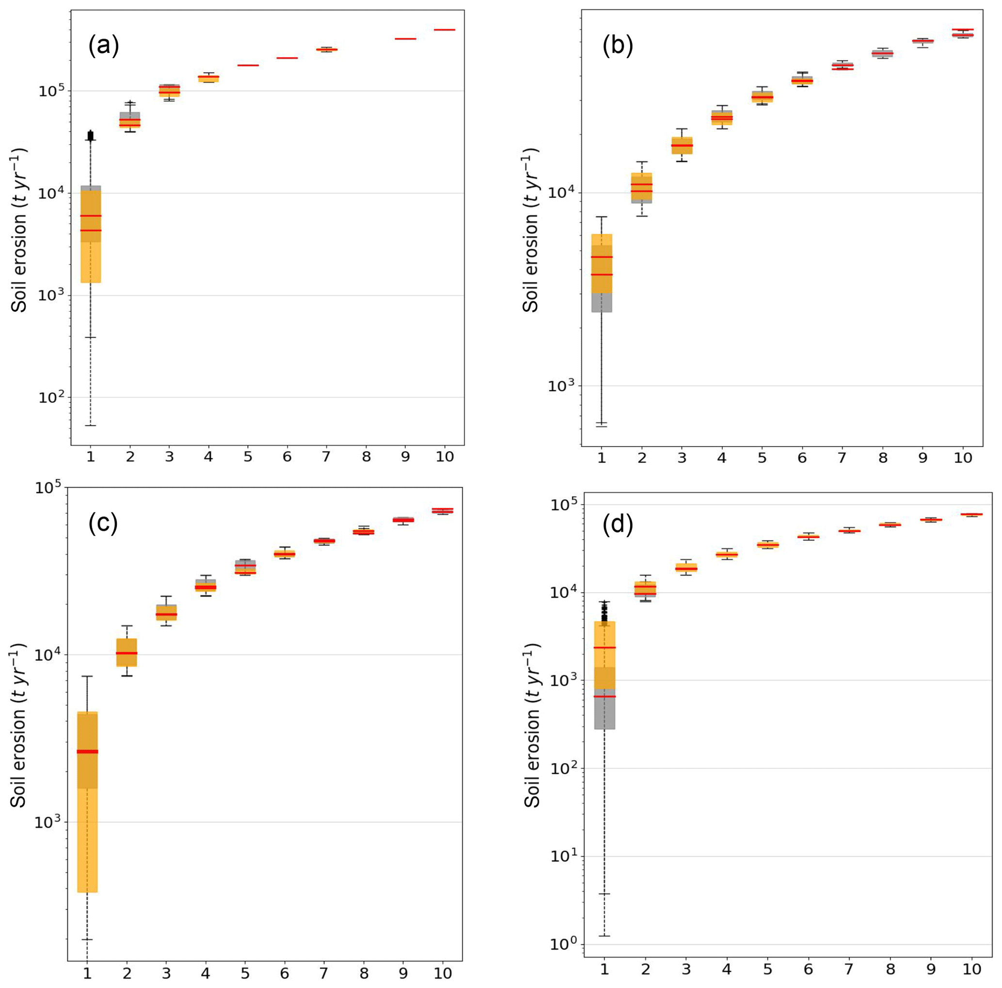
Figure 3 Quantile box-and-whisker plots of simulated gross soil erosion rates (t yr⁻¹) (gray box-and-whisker plots) compared to (a) the study by Cerdan et al. (2010), (b) the study by Panagos et al. (2015), and (c) the German potential erosion map by Bug et al. (2014) (orange box-and-whisker plots). (d) Quantile box-and-whisker plots of simulated net soil erosion rates (t yr⁻¹) (gray box-and-whisker plots) compared to the study by Borrelli et al. (2018) (orange box-and-whisker plots). Medians are plotted as red horizontal lines. The x axis represents bins or evenly spaced ranges between the minimum and maximum total yearly soil erosion rates of the Rhine derived from the data of (a) Cerdan et al. (2010), (b) Panagos et al. (2015), (c) Bug et al. (2014), and (d) Borrelli et al. (2018).

We also find that the quantile distribution of the simulated net soil erosion from hillslopes compares well with the distribution from the high-resolution modeling study by Borrelli et al. (2018) (Fig. 3d). In addition we performed a spatial comparison of our simulated gross and net erosion rates to those of the studies mentioned above. For this purpose, we delineated 13 subbasins in the Rhine catchment (Fig. S3 in the Supplement). Table 3 summarizes the resulting goodness-of-fit statistics of this comparison and shows that for gross soil erosion our erosion model is generally in good agreement with the other studies at subbasin level. However, for net soil erosion, our model results are different to those of the study by Borrelli et al. (2018) due to the different approaches in calculating the sediment deposition. For example, in our study the deposition of sediment in hillslopes is explicitly calculated as a function of the slope and vegetation type or cover. Borrelli et al. (2018) used the transport capacity concept (Van Rompaey et al., 2001). Both methods have their uncertainties when applied at large spatial scales. The method in our study has been designed and calibrated to be used at a large spatial scale and at coarse resolution, while the method of Borrelli et al. (2018) was originally designed to be applied at spatial scales <100 m.

Table 3 Goodness-of-fit results of the comparison of the simulated gross and net erosion rates to those of other studies at subbasin level, taking into account 13 subbasins of the Rhine. RMSE is the root mean square error in 10⁶ t yr⁻¹. E stands for soil erosion.

We find that the quantile distributions of our simulated agricultural C erosion and deposition rates are similar to those of the high-resolution modeling study by Lugato et al. (2018) (Fig. 4a–d). Also the spatial variability of the C erosion rates at subbasin level is in good comparison to the validation data (Table 4). However, the linear regression between soil erosion and C erosion rates of our study lies at the lower end of the relationships derived from the enhanced and reduced erosion scenarios of Lugato et al. (2018) (Fig. 5). On the one hand, our study does not include EC practices, leading to substantially larger simulated soil erosion rates in regions with EC. Figure 5 shows that our simulated erosion rates are in general larger than the erosion rates from Lugato et al. (2018), which may be explained by this mechanism. On the other hand, the C erosion rates of our study are lower than those of Lugato et al. (2018), due to the coarse spatial resolution of our underlying C scheme derived from the ORCHIDEE LSM. The decreased spread in our simulated values is also a result of the coarse resolution of our model.

Table 4 Goodness-of-fit results of the comparison of the simulated gross and net C erosion rates to those of the study by Lugato et al. (2018) in the enhanced and reduced scenario, taking into account 13 subbasins of the Rhine. RMSE is the root mean square error in t yr⁻¹. C_e stands for gross C erosion, while C_d stands for net C erosion.

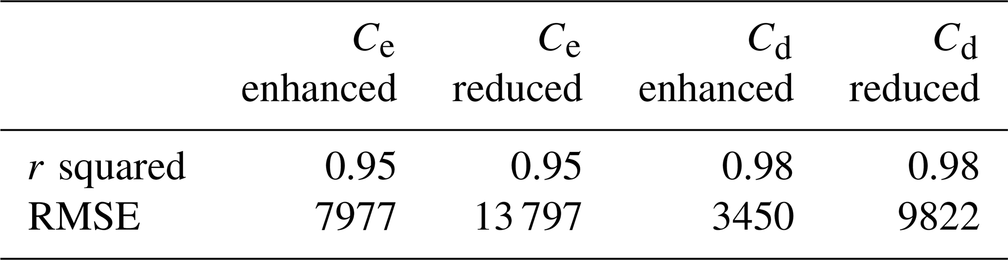
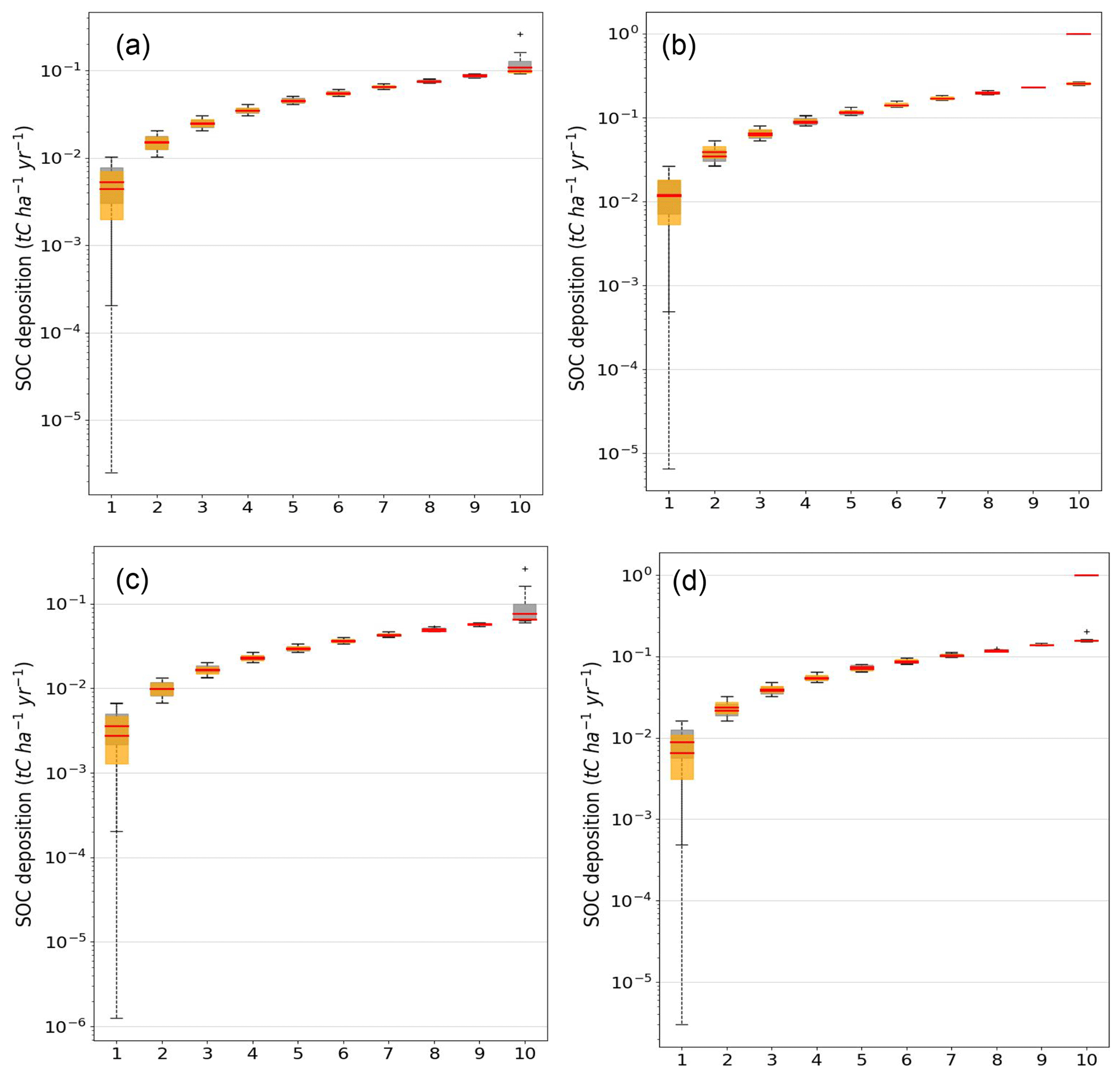
Figure 4 (a) Hillslope C erosion rates and (b) C deposition rates compared to the enhanced erosion scenario from Lugato et al. (2018). (c) Hillslope C erosion rates and (d) C deposition rates compared to the reduced erosion scenario from Lugato et al. (2018). The x axis represents bins or evenly spaced ranges between the minimum and maximum total yearly soil erosion rates of the Rhine.

Accounting for erosion, deposition, and transport of SOC leads to a better representation of the simulated topsoil C stocks per land cover type when compared to SOC stocks of the LUCAS database (Fig. 6). The simulated SOC stocks of the top 20 cm of the soil profile fall within the quantile range of the LUCAS SOC stocks for cropland and forest (Fig. 6). Although the topsoil SOC stocks for grassland improved, a large uncertainty range remains. Furthermore, we find that in both the erosion and no-erosion simulations the SOC stocks for grassland are higher than for forest. This is also observed in the study by Wiesmeier et al. (2012), where they found considerably higher SOC stocks for grassland with a median of 11.8 kg C m⁻² compared to forest based on the analysis of 1460 soil profiles in southern Germany. Furthermore, the comparison of the simulated total SOC stocks to those of the LUCAS and GSDE databases at subbasin level shows a good model performance with respect to the spatial variability in topsoil SOC stocks (Table 5).

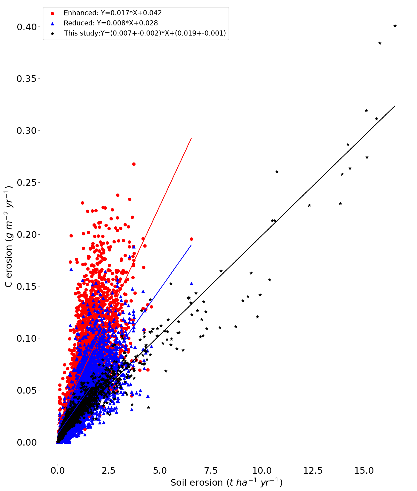
Figure 5 The relationship between soil erosion and C erosion of simulation S2 (black stars) in comparison to the erosion scenarios from the study by Lugato et al. (2018) with enhanced (red circles) and reduced erosion (blue triangles), respectively. The straight lines are the trend lines of the linear regression between soil and C erosion.

To validate the spatial variability of floodplain and hillslope SOC stocks separately, we used the scaling relationships found by Hoffmann et al. (2013a) (Sect. 2.12). We find a significantly larger exponent for the scaling relationship between the simulated floodplain SOC storage and basin area compared to the simulated hillslope SOC storage when using the grid cells that contain the points of observation corresponding to the study by Hoffmann et al. (2013a). This result is in line with what Hoffmann et al. (2013a) found, and it shows that CE-DYNAM can realistically reproduce the spatial variability in SOC stocks between hillslopes and floodplains (Table 6). However, when deriving the scaling relationships at subbasin level instead of using individual grid cells, we do not find a significant difference in the scaling between floodplains and hillslopes (Table 6).

Figure 6 Comparison of the total SOC stocks per land cover type between the simulation without erosion (red boxes with a “//” pattern), the simulation with erosion (black boxes with a “–” pattern), and the LUCAS data (green boxes without pattern fill). The red horizontal lines are the medians, the dashed vertical lines represent the range between the minimum and maximum, and the black dots are the outliers.

3.2 Model application

We find an average annual soil erosion rate of 1.44±0.82 t ha⁻¹ yr⁻¹ over the period 1850–2005, which is about half of the average erosion rate simulated for the last millennium (Naipal et al., 2016) and falls within the range of the average erosion rates of the Holocene (Hoffmann et al., 2013a). This soil erosion flux mobilized around 66±28 Tg of C over the same time period, of which on average 57 % is deposited in colluvial reservoirs, 43 % is deposited in alluvial reservoirs, and 0.2 % is exported out of the catchment.

The lower average annual soil erosion rate over the study period compared to the last millennium is a result of the general afforestation in the non-Alpine part of the Rhine catchment that started around 1910 CE according to the data on land cover and land use (Peng et al., 2017; Fig. 7b). This land cover data also shows that forest increased by 24 % over the period 1910–2005, mostly as a result of grassland-to-forest conversion. Cropland decreased by 6 % over the period 1920 to 1970 and was relatively stable afterwards. This afforestation leads to a long-term decreasing trend in gross soil and SOC erosion rates on hillslopes (Fig. 7c). The temporal variability in the soil and C erosion rates is a result of direct changes in precipitation, as is shown by the temporary increase in erosion rates over the period 1940–1960 (Fig. 7a). Furthermore, we find that the temporal variability in C erosion rates follows the soil erosion rates closely, indicating that soil erosion dominates the variations in C erosion over this time period, while increased SOC stocks due to CO₂ fertilization and afforestation play a secondary role as a slowly varying trend. It should be noted that the correlation between soil and C erosion might be affected by processes not properly captured by the model such as the selectivity of erosion including the enrichment of C in eroded material.

Table 5 This table shows the results of the linear regression between the simulated total SOC stocks (Tg C yr⁻¹) and those of the Global Soil Dataset for Earth system modeling (GSDE) and from the LUCAS database. The regression is done after aggregating the data at subbasin level for the 13 subbasins that were delineated into the Rhine catchment. RMSE is the root mean square error given in Tg C yr⁻¹, while the r value is the spatial correlation coefficient.

Table 6 This table presents the scaling exponent (b) of Eq. (20) for floodplains and hillslopes. The scaling exponent was derived for selected points in the Rhine catchment for which measurements on the SOC storage were taken by Hoffmann et al. (2013a) and at subbasin level after the data on area and SOC stocks was aggregated for each of the 13 subbasins of the Rhine.

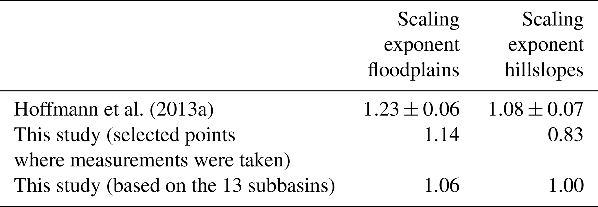
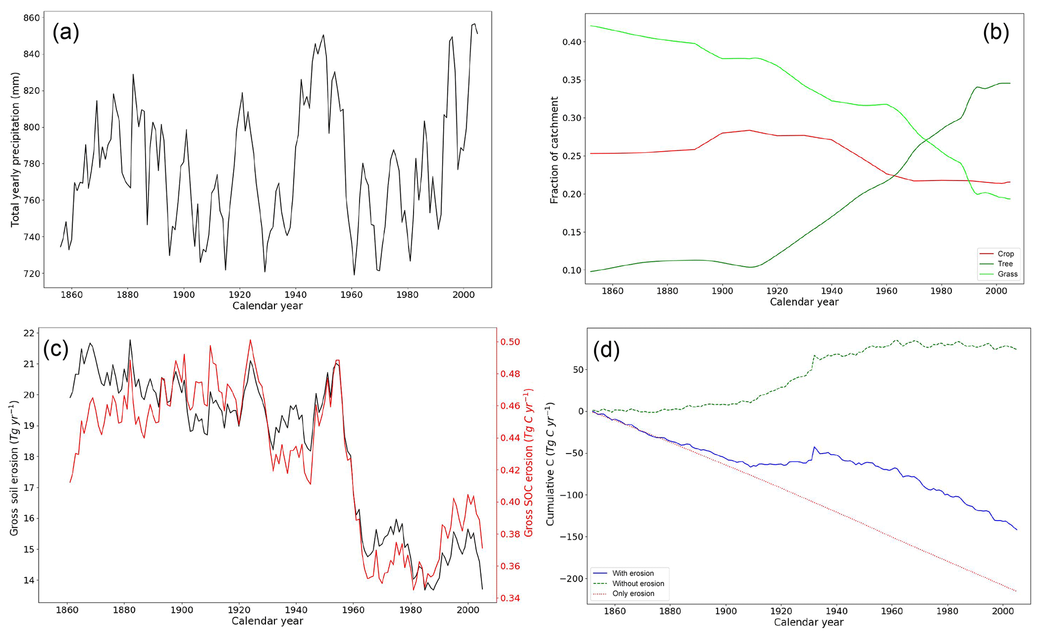
Figure 7 Time series of (a) the 5-year average yearly precipitation (mm), (b) changing land cover fractions, (c) 5-year average total gross soil erosion (Pg yr⁻¹) and total gross C erosion rates (Tg C yr⁻¹), and (d) cumulative C emissions from the soil to the atmosphere under land use change and climate change without soil erosion (dashed green line), with soil erosion (solid blue line), due to additional respiration or stabilization of buried soil and photosynthetic replacement of C under erosion (E_p, dotted red line). All graphs represent the non-Alpine region of the Rhine catchment.

The cumulative C erosion removal flux of 66±28 Tg of C leads to a cumulative net C sink for the whole Rhine region of 216±23 Tg C (Fig. 7d). This is about 2.1 %–2.7 % of the cumulative NPP and is of the same magnitude as the cumulative land C sink of the Rhine without erosion. It should be noted that these are potential fluxes, assuming that the photosynthetic replacement of C is not affected by the degradation of soil due to the removal of nutrients, declining water-holding capacity, and other negative changes to the soil structure and texture (processes not covered by our model). The breaking point in Fig. 7d around 1910 CE is a result of the climate data used as input.

To better understand the erosion-induced net C flux, we analyze the erosion-induced C exchange with the atmosphere by creating C budgets for the entire Rhine catchment for the period 1850–1860 and for the period 1950–2005 (Fig. 8a, b). These C budgets also shed light on changes in the linkage between lateral and vertical C fluxes over time. As we do not explicitly track the movement of eroded C through all reservoirs (e.g., between eroding hillslopes and colluvial reservoirs), we make use of the changes in SOC stocks and net ecosystem productivity (NEP), which is the difference between NPP and heterotrophic respiration, of the three main simulations (S0, S1, S2) to derive the erosion-induced vertical C fluxes. By subtracting the NEP of hillslopes (NEP_HS) of the no-erosion simulation (S0) from the erosion-only simulation (S1), we derive the additional photosynthetic replacement of SOC on eroding sites (Eq. 21):

$$\begin{array}{}\text{(21)}& E_{\mathrm{rep}}={\mathrm{NEP}}_{\mathrm{HS}}\left(\mathrm{S}\mathrm{1}\right)-{\mathrm{NEP}}_{\mathrm{HS}}\left(\mathrm{S}\mathrm{0}\right),\end{array}$$

where E_rep is the potential dynamic photosynthetic replacement of C on eroding sites (assuming no feedback of erosion on NPP). Part of the eroded C that is transported to and deposited in colluvial reservoirs can be respired or buried (Eq. 22). The difference between NEP of simulations S2 and S1 is the NEP caused by the deposition of eroded C in colluvial areas and equal to the difference between the burial and respiration of C in colluvial sites. As we do not explicitly track the respiration of deposited material in the model, we can only derive the net respiration or net burial of C in colluvial deposits (Rc_net) with the following equation:

$$\begin{array}{}\text{(22)}& {\mathrm{Rc}}_{\mathrm{net}}={\mathrm{NEP}}_{\mathrm{HS}}\left(\mathrm{S}\mathrm{2}\right)-{\mathrm{NEP}}_{\mathrm{HS}}\left(\mathrm{S}\mathrm{1}\right).\end{array}$$

The same concept can be applied for the net respiration or burial of floodplains:

$$\begin{array}{}\text{(23)}& {\mathrm{Ra}}_{\mathrm{net}}={\mathrm{NEP}}_{\mathrm{FL}}\left(\mathrm{S}\mathrm{2}\right)-{\mathrm{NEP}}_{\mathrm{FL}}\left(\mathrm{S}\mathrm{0}\right),\end{array}$$

where NEP_FL is the floodplain NEP, and Ra_net is the net respiration or net burial of alluvial deposits. Positive values for Ra_net or Rc_net indicate a net burial (respiration S2 < respiration S0/S1) of the deposited material.

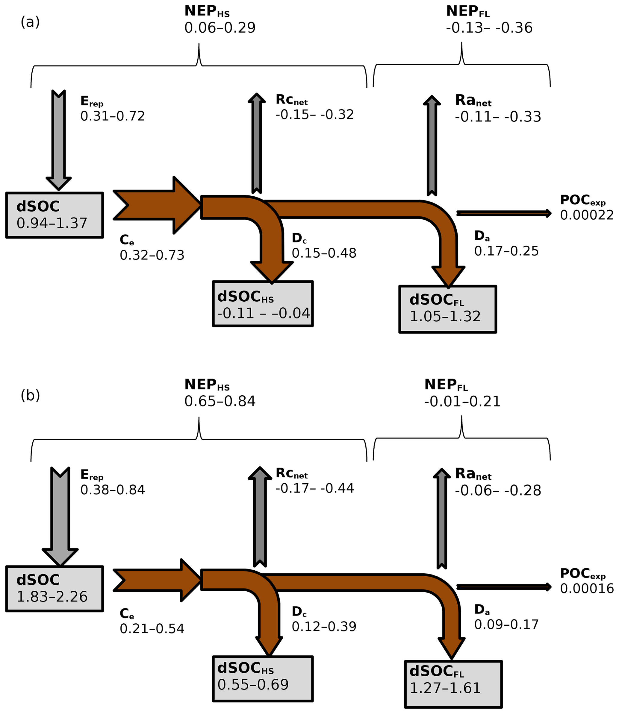
Figure 8 (a) C budget of the non-Alpine part of the Rhine for the period 1851–1861 and (b) for the period 1995–2005. The budget shows the net exchange of C (Tg C yr⁻¹) between the soil and atmosphere as a result of accelerated soil erosion rates. Gray arrows are the erosion-induced yearly-average vertical C fluxes, while the brown arrows are the erosion-induced yearly-average lateral C fluxes. C_e is gross C erosion from hillslopes; D_c is deposition of C on hillslopes; D_a is deposition of C in floodplains; POC_exp is net POC export flux; E_p is erosion-induced C replacement on hillslopes (Eq. 21); Ra_net is net respiration or burial of deposited C in floodplains (Eq. 23); Rc_net is net respiration or burial of deposited C on hillslopes (Eq. 22); NEP_HS is net ecosystem productivity of hillslopes; NEP_FL is net ecosystem productivity of floodplains. The gray boxes represent yearly-average changes in SOC stocks for the specific time period as a result of land use change, climate change, erosion, and deposition. dSOC is yearly-average change in the total SOC stock; dSOC_HS is yearly-average change in the hillslope SOC stock; dSOC_FL is yearly-average change in the floodplain SOC stock.

We find that the dynamic replacement of C on eroding sites increased by 17 %–33 % at the end of the period despite decreasing soil erosion rates (Fig. 8a, b). This increase in the photosynthetic replacement of C is due to the globally increasing CO₂ concentrations that lead to the CO₂ fertilization effect, amplified by the afforestation trend in the Rhine over this period. Without this fertilization effect, soil erosion and deposition would be likely a weaker C sink or even a C source over the period 1850–2005 (Fig. S4a, b). This CO₂ fertilization effect promotes a 100 % replacement of the eroded C on hillslopes and even leads to a C sink on hillslopes at the end of the study period (Fig. 8b). Furthermore, we find that the yearly-average gross C erosion flux from eroding sites decreases by 10 %–34 %, while the yearly deposition fluxes in colluvial and alluvial sites decreases by 20 % and 19 %–47 %, respectively. The decrease in the deposition flux to floodplains is compensated by a better sediment connectivity between hillslopes and floodplains due to afforestation. Forests have less artificial structures that can prevent the erosion fluxes from reaching the floodplains, which is represented by a higher floodplain deposition “f” factor in the model. The decrease in the erosion flux also leads to a decreased POC export of the catchment at the end of the study period.

We also find that both the colluvial and alluvial reservoirs show a net respiration flux throughout the time period (Fig. 8a, b). This is consistent with previous studies that found that deposition sites can be areas of increased CO₂ emissions (Billings et al., 2019; Van Oost et al., 2012). However, there is a slight difference in the respiration of deposited C between the start and end of the transient period. The respiration of deposited SOC in colluvial sites increases with time while the respiration of deposited SOC in alluvial sites shows rather a decreasing trend. These changes in SOC respiration of deposited material depends on (1) the amount of deposited material, (2) increasing temperatures over 1850–2005 for the entire catchment, and (3) the constant removal of C-rich topsoil and its deposition in alluvial and colluvial reservoirs, which makes the deposited sediments generally richer in C than soils on erosion-neutral sites, providing more substrate for respiration. The largest increase in total respiration of alluvial and colluvial deposits over time takes place in hilly regions due to the initial increase in erosion rates, resulting in large deposits of C. Overall, we find that the increased respiration of deposited material slightly offsets the increased dynamic C replacement; however, the dynamic C replacement on eroding sites still dominates the erosion-induced C sink.

4 Discussion

In this section we discuss some of the most important model limitations, uncertainties, and assumptions.

4.1 Initial conditions and past global changes

Initial climate, land cover or land use conditions, and the length of the transient period are essential parameters that determine the resulting spatial distribution of soil and C. Landscapes are in a constant transient state due to global changes, such as climate change, land use change, and accelerated soil erosion. However, we assumed an equilibrium state so that we can quantify the changes during the transient period. The longer the transient period that covers the essential historical environmental changes, the more accurate the present-day distribution of SOC stocks, sediment storages, and related fluxes are. This is especially true when analyzing the redistribution of soil and C as a result of erosion, deposition, and transport, as these soil processes can be very slow. For example, the study by Naipal et al. (2016) showed that by simulating the soil erosion processes for the last millennium a spatial distribution of sediment storages that is similar to observations can be found. In this study we simulated the steady state based on the initial conditions of the period 1850–1860 due to constraints in data availability on precipitation and temperature. By focusing only on the period 1850–2005 we miss the effects of significant land use changes in the past that coincided with times of strong precipitation such as in the 14th and 18th century (Bork and Lang, 2003). These major anthropogenic changes in the last Holocene substantially affected the present-day spatial distribution and size of sediment storage and SOC stocks.

The absolute value of the SOC storage from the S2 simulations of the non-Alpine region of the Rhine catchment for the year 2005 ranges between 2.74–2.99 Pg of C, which is larger than the 1.7±0.6 Pg of C that Hoffmann et al. (2013a) measured. It should be noted that the ORCHIDEE model (S0 simulation) already overestimates the total SOC stock of the non-Alpine region of the Rhine (2.43 Pg of C) when the initial conditions of the period 1850–1860 are used. Due to the fact that we miss the climate and land use changes before the year 1850, we find that floodplains store less SOC than hillslopes. Although this is in contrast to the findings by Hoffmann et al. (2013a), the difference in SOC stocks between floodplains and hillslopes from the S2 simulations is better than the difference derived from the S0 simulation. We find that floodplains store between 1.28 and 1.72 Pg of C and hillslopes store between 1.7 and 2 Pg of C when erosion and deposition processes are taken into account in comparison to 0.69 Pg of C for floodplains and 2.29 Pg of C for hillslopes when these processes are lacking.

We also find that floodplains have an overall higher C concentration (12 kg m⁻² for a 2 m soil profile) compared to hillslopes (9 kg m⁻² for a 2 m soil profile) at the end of the transient period (Fig. 9a), which is in line with the findings by Hoffmann et al. (2013a) and what can be derived from global soil databases. This is a result of higher SOC concentrations in deeper soil layers of floodplains compared to hillslopes (Fig. 9a, b), as is also shown in the study by Hoffmann et al. (2013a). To be closer to the observational difference between floodplains and hillslopes, we would need to consider the period before the year 1850, extreme climate events, and a higher plant productivity in floodplains resulting from favorable soil nutrient and hydrological conditions.

Figure 9 (a) Vertical distribution of hillslope (red) and floodplain (blue) SOC stocks (kg m⁻²) with depth averaged over the non-Alpine region of the Rhine catchment and (b) the vertical distribution of normalized hillslope (red) and floodplain (blue) SOC stocks (dimensionless) with depth.

4.2 Model advantages and limitations

Although we parameterized and applied CE-DYNAM for the Rhine catchment, it is intended to be made applicable to other large catchments. CE-DYNAM combines soil erosion processes, for which small-scale differences in topography are of utter importance, with a state-of-the-art representation of large-scale SOC dynamics driven by land use and environmental factors (climate, atmospheric CO₂) as simulated by the ORCHIDEE LSM. The flexible structure of CE-DYNAM makes the model adaptable to the SOC dynamics of other LSMs. In this way, it is possible to study the main processes behind the linkages between soil erosion and the global C cycle.

CE-DYNAM explicitly accounts for hillslope and floodplain redeposition, which is to our knowledge unique for a large-scale C erosion model and highly novel. However, it still lacks important processes affecting the C dynamics in floodplains. The model does not account for a slower respiration rate due to low-oxygen conditions or physical and chemical stabilization (Berhe et al., 2008; Martínez-Mena et al., 2019). The oxidation and preservation of C in deposition environments, especially in alluvial reservoirs, remain highly uncertain (Billings et al., 2019).

Due to its simplistic nature and coarse resolution, CE-DYNAM does not resolve rivers and streams explicitly but assumes that they are included in the floodplain part of the grid cells. As a result, CE-DYNAM does not differentiate between eroded hillslope soil that reaches the water network directly (where the residence time of suspended sediment is on the order of days) or the sediment that is first retained in the floodplains before it reaches the water network due to fluvial erosion (sediment residence time is on the order of a few years to thousands of years). CE-DYNAM has been developed and calibrated to simulate long-term changes in sediment and C storage on land and not the short-term variations in sediment and POC fluxes carried by rivers. This limits the application of CE-DYNAM in its current form to accurately quantify sediment and POC fluxes of rivers and streams, as well as to compare them to observations.

As a result of the abovementioned model limitation, CE-DYNAM produces a sediment export flux at the end of the year 2005 of about 6472 t yr⁻¹, which is about 2 orders of magnitude lower than the estimated suspended sediment flux of about 3.15×10⁶ t yr⁻¹ from Asselman et al. (2003) or the 0.75×10⁶ t yr⁻¹ simulated by Li et al. (2020). This sediment export rate leads to a yearly sediment-bound POC export of about 2×10⁸ g C yr⁻¹ in 2005. This POC flux is also 2 orders of magnitude lower than the 2.6×10¹⁰ g C yr⁻¹ given by the GlobalNEWS2 model (Mayorga et al., 2010) or the 1.5×10¹¹ g C yr⁻¹ found by Beusen et al. (2005), which is mainly a result of the underestimated simulated sediment export rate.

Furthermore, CE-DYNAM does not simulate fluvial erosion as a complex function of the channel geometry, riverbank erodibility, or shear stress (Dröge et al., 1992), due to the lack of data on these parameters at the regional scale and to keep a balance between model complexity and its computational ability. Also, our model does not resolve erosion of the deposited river sediment by flooding events. This simplified model concept for fluvial erosion contributes to the underestimation of sediment and C export in floodplains. Finally, with the current model setup, we do not account for large soil erosion events before 1850 CE or extreme precipitation events that may have a long-term effect on the sediment export rate of the Rhine.

Although we underestimate the riverine sediment and POC fluxes, we find that the spatial variability in sediment storage and SOC stocks of the subbasins are within or close to observational uncertainty ranges (Tables 5, 6; Naipal et al., 2016). We also find that the C density in the topsoil layers of floodplain soils located downstream of the Rhine and the C concentration of the POC flux are realistic. We find a C concentration of ∼3.3 % in the exported fine sediments downstream of the Rhine. Abril and Borges (2005) found a 5.5 % POC mass fraction in suspended sediments for the Rhine. The C density of the topsoil layer of the floodplains in the downstream grid cells in the S2 simulations (S2, S2_min, S2_max) is on average 4.47 kg C m⁻², which falls within the range of the average C density of 5.13±1.3 kg C m⁻² measured by Hoffmann et al. (2013a) for floodplain overbank deposits. By comparison, the average C density of the topsoil layers of downstream grid cells in the S0 simulation is 12.78 kg C m⁻², which is an overestimation. Other model uncertainties that may affect the SOC stocks and POC fluxes include the absence of increased plant productivity of floodplains and transformations between POC, DOC, and CO₂ and their fate in rivers and streams. Increased plant productivity of floodplains is shown to contribute significantly to the higher SOC stocks of floodplains compared to hillslopes and to the export of DOC and POC to rivers (Van Oost et al., 2012; Hoffmann et al., 2013a).

In a future study we aim to improve the sediment and POC export and account for a higher floodplain plant productivity by using a nutrient-enabled version of the ORCHIDEE LSM (Goll et al., 2017).

Furthermore, the model does not take into account the full effects of the selectivity of erosion, often expressed as the enrichment ratio, where the C content of eroding soil or the deposited sediment can be different from that of the original soil. The enrichment ratio varies substantially across landscapes, while the importance of erosion selectivity for C is still under debate (Nadeu et al., 2015; Wang et al., 2010). However, we did a simple sensitivity test to study the effect of C enrichment by erosion (Sect. 4.3).

CE-DYNAM does not account for different ratios between the SOC pools (active, slow, passive) with depth due to the limitation in information to constrain these fractions for floodplains and hillslopes. However, this can be potentially important for respiration of C in depositional sites and during transport. Studies show that the labile C is decomposed first during sediment transport and directly after deposition, leaving behind the more recalcitrant C in deposition sites (Berhe et al., 2007; Billings et al., 2019). Due to the simplistic nature of our coarse-resolution model and the lack of data on oxidation of eroded C during transport, we did not include C respiration during transport in the model.

The current SOC scheme of CE-DYNAM does also not account for different residence times of SOC as a function of landscape position along a hillslope. The SOC decomposition rates can vary significantly along a hillslope due to changes in soil moisture, temperature, aggregation, and the transport of minerals and nutrients (Doetterl et al., 2016). Currently, these processes are not resolved in coarse-resolution LSMs, contributing to the uncertainty in the large-scale linkage between soil erosion and SOC dynamics.

Furthermore, there is no feedback between soil erosion and plant productivity in the model. To account for this feedback, soil erosion processes would need to be explicitly included in a LSM, such as ORCHIDEE, which would increase the computational complexity of the simulations substantially. The lack of this feedback results in an unlimited dynamic replacement of C on eroding sites.

Currently, the erosion scheme of CE-DYNAM does not include the L (slope-length) and P (support-practice) factors. This might induce some bias in the results, especially for agricultural land. In a future study we aim to make CE-DYNAM better applicable for agricultural land, where these factors play an important role. For this purpose, we will focus on the development of new methods that can quantify the L and P factors reliably at the global scale, and we will need to recalibrate the Adj.RUSLE model. Our decision of leaving out the Land P factors from the erosion equation in this study is based on the global study by Doetterl et al. (2012), which showed that the S, R, Cm, and K factors explain approximately 78 % of the total erosion rates on cropland in the USA. This indicates that on cropland the L and P factors, which are related to agriculture and land management, contribute only 22 % to the overall erosion rates. This percentage is comparable to the uncertainty range in the estimation of the S, R, Cm, and K factors at the regional scale from coarse-resolution data. Renard and Ferreira (1993) also mention that the soil loss estimates are less sensitive to slope length than to most other factors. Furthermore, various studies argue that the estimation of the L factor for large areas is complicated and thus can induce significant uncertainty in soil erosion rates calculated based on coarse-resolution data (Foster et al., 2002; Kinnell, 2007). Especially for natural landscapes, such as forests, the estimation of the L factor is not straightforward as these natural landscapes usually include steep slopes (Elliot, 2004). In order to stay consistent with the estimation of potential soil erosion for all land cover types, we removed the L factor from the equation. The Adj.RUSLE has been already successfully validated at the regional scale, without the L and P factors, where the spatial variability of soil erosion rates compared well to other high-resolution modeling studies and observational data, and where the absolute values fell within the uncertainty ranges of those validation data (Naipal et al., 2015, 2016, 2018; and this study). Finally, the aim of this study was to develop and validate a C erosion scheme for applications at the global scale, where the estimation of the L and P factors is limited. By showing that the erosion rates from the Adj.RUSLE and CE-DYNAM are within the uncertainty of other data and modeling studies, we assume that it will be applicable for other large catchments in the temperate region.

Finally, CE-DYNAM considers only the rather “slow” rill and interrill soil erosion processes, and it does not take into account severe erosion processes such as gully erosion and landslides, which are bound to extreme precipitation events. The daily time step of CE-DYNAM and the current setup of the sediment budget module only allows for long-term yearly-average changes in erosion and deposition rates and cannot be applied to estimate episodic erosion and deposition events.

4.3 Sensitivity analysis

We analyzed the effects of the following model assumptions: (1) C enrichment during erosion, (2) the floodplain sediment residence time, and (3) crop residue management.

To test the C enrichment, we increased the EF parameter (Eq. 15) from 1 to 2, assuming a strong enrichment of C during erosion (Sect. 2.11). We find that this enrichment results in a gross C erosion flux that is 1.61 times larger than the flux without enrichment (Table 7). This leads also to a larger dynamic replacement of C on eroding sites in combination with a larger burial in depositional sites, which is in accordance with the study by Lugato et al. (2018). The resulting C sink from the enrichment simulation is 1.25 times larger than the sink under default conditions (Table 7).

Table 7 Sensitivity analysis. The impacts of enrichment, changes to the sediment residence time (τmin,τmax), and crop residue management (RM) on the cumulative gross C erosion (C_e), the cumulative change in the total SOC stock (dSOC), the net C sink, and the cumulative particulate organic C export flux (POC_exp) of the Rhine catchment (units: Tg C).

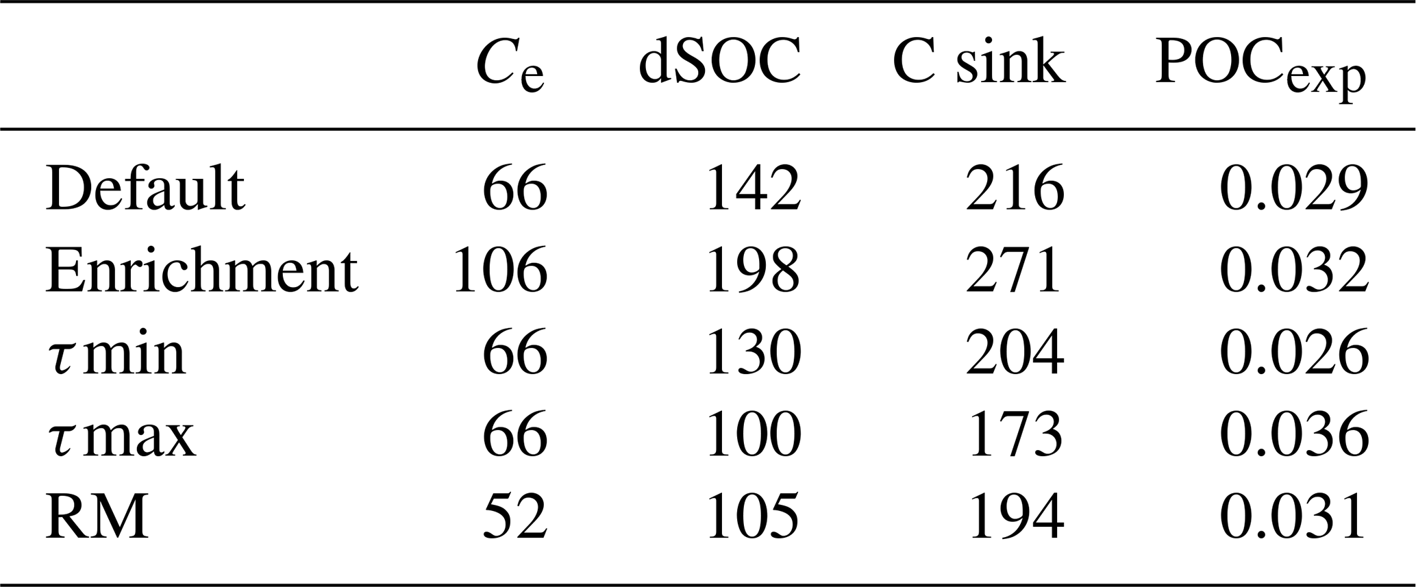
To test the potential effects of a different sediment residence time on the SOC dynamics, we performed a sensitivity study where we changed the basin average sediment residence time to be 50 % higher or 50 % lower but kept the maximum sediment residence time at 1500 years (Sect. 2.11). By changing the average sediment residence time and keeping the maximum fixed, the grid cells with the lowest residence times underwent the largest changes in the residence time and consequently in the floodplain SOC storage and export. The higher the residence time, the longer the deposited soil C will reside in the floodplains, where it can either be respired or buried in deeper soil layers. Therefore, we find that the effects of the sediment residence time on the SOC dynamics are nonlinear. Under default conditions we find the highest SOC storage. A 50 % higher average sediment residence time leads to the lowest total SOC storage, with a decrease of 30 % compared to default conditions, while the erosional C sink is reduced by 20 % (Table 7). This could be explained by a higher C decomposition flux for floodplains due to the long residence time of C in deposition areas. Especially in mountainous regions where the soil erosion flux is large and removes a large part of the labile C, a higher sediment residence time will lead to higher C emissions due to decomposition in floodplains. The turnover seems to dominate over the C burial in deeper layers and export. A 50 % lower average sediment residence time also leads to a decrease of 8 % in the total SOC storage and a decrease of 6 % in the erosional C sink compared to default conditions (Table 7). Also here, the largest changes are found in mountainous regions where a low sediment residence time leads to a large export of C, which is then deposited in lower lying, more extensive floodplains. Thus, increasing or decreasing the residence time leads to a smaller total SOC storage, resulting from different spatial distributions of this SOC storage. The POC flux under the high sediment residence time scenario is substantially higher than under default conditions (Table 7).

To test the effects of crop residue management, we harvested all aboveground crop residues (Sect. 2.11). We find that the total litter C stock is about 15 % smaller than the default case by the end of the year 2005. This leads to a total change in the transient SOC stocks that is 20 % smaller under no erosion (S0), and 26 % smaller under erosion (S2) (Table 7). Our findings confirm that soil management practices such as residue management have a substantial effect on the SOC dynamics.

5 Conclusions

We presented a novel spatially explicit and process-based C erosion dynamics model, CE-DYNAM, which simulates the redistribution of soil and C over land as a result of water erosion and estimates the implications for C budgets at catchment scale. We demonstrated that CE-DYNAM captures the spatial variability in soil erosion, C erosion, and SOC stocks of the non-Alpine region of the Rhine catchment when compared to high-resolution estimates and observations. We also showed that the quantile ranges of erosion and deposition rates and C stocks fall within the uncertainty ranges of previous estimates at basin or subbasin levels. Furthermore, we demonstrated the model's ability to disentangle vertical C fluxes, resulting from the redistribution of C over land and develop C budgets that shed light on the role of erosion in the C cycle. The simple structure of CE-DYNAM and the relatively low number of parameters make it possible to run several simulations to investigate the role of individual processes on the C cycle such as the removal by erosion only or the role of sediment deposition and transport. Its compatibility with land surface models makes it possible to investigate the long-term and large-scale effects of erosion processes under various global changes such as increasing atmospheric CO₂ concentrations, changes to precipitation and temperature, and land use change.

The application of CE-DYNAM for the Rhine catchment for the period 1850–2005 CE reveals three key findings.

Soil erosion leads to a cumulative net C sink of 216±23 Tg of C by the end of the period, which is on the same order of magnitude as the cumulative land C sink of the Rhine without erosion. This C sink is a result of an increasing dynamic replacement of C on eroding sites due to the CO₂ fertilization effect, despite decreasing soil and C erosion rates over the largest part of the catchment. We conclude that it is important to take into account global changes such as climate change in order to better quantify the net effect of erosion on the C cycle.

After performing a sensitivity analysis on key model parameters we find that the C enrichment by erosion, crop residue management, and the residence time of floodplain sediment can substantially change the overall values of C fluxes and SOC storages. However, the main findings, such as soil erosion being a net C sink for the Rhine catchment, remain.

Initial climate and land cover conditions and the transient period over which erosion under global changes takes place are essential for determining if soil erosion is a net C sink or source and to what extent.

Altogether, these results indicate that despite model uncertainties related to the relatively coarse spatial resolution and missing or simplified processes, CE-DYNAM represents an important step forwards to integrating soil erosion processes and sediment dynamics in Earth system models. The next step would be to improve CE-DYNAM with respect to riverine sediment and POC export fluxes and management practices.