GLOBAL-FATE (version 1.0.0): A geographical information system (GIS)-based model for assessing contaminants fate in the global river network

GLOBAL-FATE is the first open-source, multiplatform, user-friendly, and modular contaminant-fate model operating at the global scale linking human consumption of pharmaceutical-like compounds with their concentration in the river network. GLOBAL-FATE simulates human consumption and excretion of pharmaceuticals, the attenuation of the contaminant load in waste water treatment plants as well as the attenuation of the contaminant load in river reaches, lakes, and reservoirs as a first-order decay depending on residence time. We provide a comprehensive description of model equations and the overall structure of the model, with special attention to input–output datasets. GLOBAL-FATE is written in C, can be compiled in any platform, and uses inputs in standard geographical information system (GIS) format. Additionally, the model can be run in the Quantum Geographic Information System (QGIS) as a plug-in. The model has no built-in working resolution, which depends on the intended use and the availability of appropriate model inputs and observed data. We exemplify the application of GLOBAL-FATE solving the global concentration of diclofenac in the river network. A comparison with a dataset of diclofenac concentration observations in rivers suggests that GLOBAL-FATE can be successfully applied in real-case modelling exercises. The model is particularly sensitive to the generation of contaminant loads by human pharmaceutical consumption and to the processes governing contaminant attenuation in the river network. GLOBAL-FATE will be a valuable tool for the scientific community and the policymaking arena and could be used to test the effectiveness of large-scale management strategies related to pharmaceutical consumption control and waste water treatment implementation and upgrading.

1 Introduction

The United Nations 2030 Agenda for Sustainable Development identifies 17 master goals, amongst which is the availability and sustainable management of water and sanitation. This agenda establishes as a goal the improvement of water quality by reducing pollution, eliminating dumping, and minimizing release of hazardous chemicals to the river network by 2030 (UN General Assembly, 2015). However, a large proportion of surface water networks is currently severely affected by sewage inputs from waste water treatment plants (WWTPs) or by direct sewage disposal (Richardson et al., 2005; Stewart et al., 2014; Hernández et al., 2015; K'oreje et al., 2016). Sewage disposal inputs organic matter, nutrients, and faecal bacteria into the river network, together with a whole plethora of chemicals related to human household activities. These include microplastics and nanomaterials (Besseling et al., 2017), pharmaceuticals (Li et al., 2016), personal care products (Arlos et al., 2014), and even illegal drugs (Postigo et al., 2010). These down-the-drain chemicals reach the river network and affect both humans and biodiversity and ecosystem function (Rudd, 1970), thus posing a risk to water security (Goldman and Koduru, 2000; Vörösmarty et al., 2010).

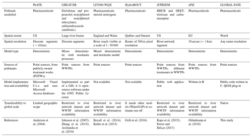
Assessing chemical discharges and their fate in the river network is thus vital for evaluating both the health of aquatic ecosystems and the security of water supplies for human needs. This requires adequate models to consider the spread and dynamics of chemicals at large spatial scales, both for assessing the current water quality status in regions with poor monitoring programme coverage (Strokal et al., 2019), and for planning management and mitigation measures. Existing models approach the fate of contaminants in multimedia (air, water, soil) and using steady-state models working at regional scales such as ChemCAN, HAZCHEM, or EUSES (MacLeod et al., 2011; Gouin et al., 2013; Lindim et al., 2016). Others are process-based, operating at the watershed scale, and perform as dynamical in-stream water quality models, such as MIKE11, SWAT, WASP, QUAL2E, or DELWAQ (Liang et al., 2015; Santhi et al., 2005; Di Toro et al., 1983; Brown et al., 1987; Van Wijngaarden, 1999). Another set of models analyse the dynamics of down-the-drain pollutants, considering the linkages between engineered systems (e.g. WWTPs) and natural systems (e.g. rivers). This includes PhATE, GREAT-ER, LF2000-WQX, STREAM-EU, iSTREEM, and ePiE (Anderson et al., 2004; Feijtel et al., 1997; Johnson et al., 2007; Boxall et al., 2014; Lindim et al., 2016; Kapo et al., 2016, Oldenkamp et al., 2018) that are frequently targeting pharmaceutical products, although they are also suitable to simulate the fate of any compound decreasing following first-order decay dynamics (Table 1). Particularly, models in Table 1 are applied for chemicals whose dominant emission source to the environment is via WWTP effluents. Most of these models are highly data demanding and use many adjustable parameters. This makes some of them computationally inefficient; others have non-open-source codes, which make their use for global- or continental-scale calculations cumbersome.

Table 1 Features of a collection of contaminants fate models compared to those of GLOBAL-FATE.

Recently, other approaches specifically designed for very large scales have used a geographical information system (GIS) framework to solve the routing of chemicals along the river network (Pistocchi et al., 2012; Dumont et al., 2015; Grill et al., 2016; Rice and Westerhoff, 2017). Most of these models use a much simpler model parameterization in order to make continental and global calculations accessible. However, some of them assume that chemicals do not decay when travelling through the river network and simply rely on dilution factors once pollutants enter the river network. Further, they work at a fixed spatial scale, which is either very coarse to adequately represent the river network (e.g. 0.5^∘) or is too detailed to be practical for global calculations due to computational requirements (e.g. 500 m; Grill et al., 2018).

GLOBAL-FATE has been designed to overcome these constraints, offering the first contaminant-fate model operating in the global river network, including lakes and reservoirs, which is at the same time open-source, multiplatform, user-friendly, and modular. This will make global contaminant calculations accessible to a much wider community of scientists and practitioners, opening the door for including pharmaceutical pollution in influential assessments of climate change impacts (e.g. the Inter-Sectoral Impact Model Intercomparison project) and global policy instruments like the UN Sustainable Development Goals agenda. GLOBAL-FATE calculates the steady-state concentration of a user-defined down-the-drain contaminant through the global river network, including lakes and reservoirs. GLOBAL-FATE is offered as an open-source, GIS-based model programmed in the C language, allowing researchers to select the input information (water routing, hydrology, population, etc.) and the spatial resolution at which the model has to perform. Thus, the model can include new or different hydrological datasets and other input information, and hence it is not fundamentally restricted to a single modelling resolution or hydrological or socio-economic scenario. The model simulates the propagation of down-the-drain contaminants along the river network, and the constituent decreases at a rate proportional to its concentration in the aquatic media. GLOBAL-FATE is also computationally efficient, can be run in Windows or Linux machines, and can take advantage of parallel computing in multi-processor computers or clusters. It can also be run as a user-friendly plug-in in the Quantum Geographic Information System (QGIS), and the modular structure of its code allows switching different functions of the model on and off. Here we describe the structure, functioning, and strengths and limitations of GLOBAL-FATE. First, we explain the structure and functioning of the model, focusing on the type of input data structure and the formulation of the different hydrological and biogeochemical processes. Then, the application of the model is exemplified solving the worldwide propagation of the pharmaceutical diclofenac throughout the global river network. Finally, we discuss strengths and limitations of GLOBAL-FATE and point to future developments.

2 Methodology

GLOBAL-FATE is a physically based model for simulating constituent inputs to the river network and their routing along the river network at the global scale. Our approach shares key assumptions and modelling mechanisms with other large-scale pharmaceutical models for the river network (i.e. Keller et al., 2006; Pistocchi, 2014; Grill et al., 2018), including the use of per capita mass emissions of the contaminant of interest, simplified parameterization of losses due to human metabolism and removal in waste water treatment plants, and dilution and first-order attenuation dynamics upon discharge into natural waters. However, GLOBAL-FATE is the first model natively operating at the global scale including all those mechanisms, including explicit routing and attenuation in lakes and reservoirs.

The model uses GIS input files to solve for the contaminant fate at every element (cell) of the domain (raster). The model is multiplatform, written in C, and uses multi-core parallel computing via OpenMP. Additionally, GLOBAL-FATE can be used from QGIS (QGIS Development Team, 2018) as a plug-in, so it can be executed in a push-button fashion, in order to load all the layers and information the model needs in a user-friendly way, as well as automatically producing basic visualizations of the results. The code (including compilation instructions) is freely available at https://doi.org/10.5281/zenodo.3524124, including the QGIS plug-in. Pre-built executables are available on request.

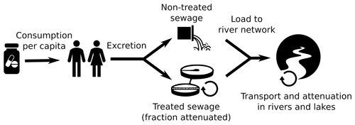
GLOBAL-FATE simulates the fate of contaminants that behave like human pharmaceuticals (Fig. 1). That is, the model assumes that the origin of the contaminant load is the consumption of a pharmaceutical by population, which can differ in different regions of the world considering population density and per capita consumption. No other origins, such as diffuse sources through the spreading of pharmaceutical-rich farm manure on agricultural fields, are currently included. The model assumes an excretion rate by population, and the fraction finally excreted will reach the river network either directly or after some attenuation in WWTPs. The fraction of load treated can be dependent on the region of the world, while the decay in WWTPs is an input parameter that applies globally. Finally, the contaminant load is routed along the river network, considering that the contaminant will decay following first-order kinetics dependent on water residence time in the river network reaches. GLOBAL-FATE also considers the presence of lakes and reservoirs in the river network and includes a particular solution for water residence time in these systems in order to calculate contaminant decay. The main output is a global map of predicted contaminant load or concentration throughout the river network.

Figure 1 Conceptual diagram of the processes modelled by GLOBAL-FATE.

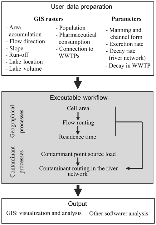
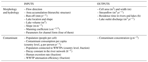
The model workflow (Fig. 2) is based on the input of nine global maps in the form of raster datasets and the definition of eight parameters (Table 2). The model has been designed to work with raster data with the geographic coordinate system WGS84 in decimal degrees, but it does not have a predefined spatial resolution. The only prerequisite is that all input rasters must have the same resolution and extent. Raster input data files are expected to have an ASCII ESRI (http://resources.esri.com/help/9.3/arcgisdesktop/com/gp_toolref/spatial_analyst_tools/esri_ascii_raster_format.htm, last access: 27 November 2019) grid format, which makes GLOBAL-FATE very easy to set up using customary GIS software even for non-experienced users.

Figure 2 Work flow of GLOBAL-FATE.

Table 2 Input and output datasets and parameters for both geographical (morphology and hydrology) and contaminant model processes.

2.1 Model workflow

The model is composed of six main functions that are executed successively, with some outputs being the inputs to the next function. First, the geographically related functions are run, which deliver streamflow and water residence time along the river network as main outputs. Then, the contaminant-related functions calculate the load of contaminant to the river network by population, after discounting for waste water treatment and also the routing of the contaminant through the river network considering that the contaminant decays following a first-order reaction dynamics. The following is a description of the calculations performed by the six main functions in GLOBAL-FATE (see also Table 3 and the code and example input files at the GitHub repository).

Table 3 Main calculation steps in GLOBAL-FATE, with indication of inputs and outputs used by each process, and the C functions responsible. Outputs with an asterisks can be saved during model execution and accessed afterwards.

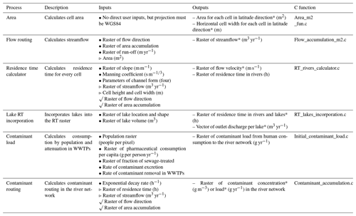
Input flag legend: • dataset used for the first time; ▹ input coming from previous function output; √ dataset used (at least) for the second time.

2.1.1 Cell area (function Area_m2_fun.c)

This function performs an auxiliary calculation for the flow routing function. In order to route locally generated run-off, the area (m²) of each cell in the domain is necessary. Considering WGS84 as a reference coordinate system, cell height is the length of the arc formed by the angle δ (raster resolution in decimal degrees transformed to radians) and is constant in the whole grid, calculated as

$$\begin{array}{}\text{(1)}& H=\mathit{\delta }R,\end{array}$$

where R is the authalic Earth radius (6 371 007.2 m). In turn, the width of each cell depends on latitude:

$$\begin{array}{}\text{(2)}& W\left(y\right)=R\left(\sin \left(y+{\displaystyle \frac{\mathit{\delta }}{\mathrm{2}}}\right)-\sin \left(y-{\displaystyle \frac{\mathit{\delta }}{\mathrm{2}}}\right)\right).\end{array}$$

Here y corresponds to the latitude and comes from

$$\begin{array}{}\text{(3)}& y=y_{\mathrm{0}}+\mathit{\delta }\left(\mathrm{nr}-j\right),j=\mathrm{1},\mathrm{\dots },\mathrm{nr},\end{array}$$

where y₀ is the southern cell latitude and nr is the number of rows in the raster, so j is a latitude index. Due to the fact that cells at the same latitude have equal width, both area (m²) and width are calculated for one meridian:

$$\begin{array}{}\text{(4)}& A\left(y\right)=H\cdot W\left(y\right).\end{array}$$

2.1.2 Flow routing (function Flow_accumulation_m2.c)

Streamflow in each cell of the raster is computed using a run-off accumulation approach. First, for each basin, cells are enumerated from headwaters (l=0) to river mouth (l=L), following the hierarchical organization of the river network. The J_l is the set of cell indexes at stages $l=\mathrm{0},\mathrm{\dots },L$. This cell classification is obtained as a raster input dataset (Table 3) and is a typical product of many GIS hydrological algorithms (often defined as an area or flow accumulation layer). Second, we define the amount of run-off locally generated in each cell due to the precipitation–evaporation water budget. For this, we use available products of mean annual run-off (m yr⁻¹) at the global scale in raster format, rescaled to the same resolution as the rest of the hydrological input rasters. Finally, we route the locally generated run-off along the river network following the hierarchical order defined in the first step. Streamflow in cell j in J_l>0 is computed as the sum of run-off inputs from the surrounding cells and that generated within the cell. In order to determine the input from the neighbouring cells, a raster of flow direction is used. Such a raster must be encoded following the D8 method (O'Callaghan et al., 1984). Finally, average annual streamflow in cubic metres per year in each cell is calculated after summing up the multiplication of cell run-off (m yr⁻¹) by the corresponding cell area (Eq. 4, m²):

$$\begin{array}{}\text{(5)}& q_j={\sum }_{i\in N_j}{q}_i+{\text{run-off}}_j{A}_j,j\in J_{l>\mathrm{0}},\end{array}$$

where $N_j\subseteq J_{l-\mathrm{1}}$ is the set of indexes of the neighbourhood of cell j such that i∈N_j implies that the flow of cell i goes to cell j and A_j is the area of cell j. Note that for l=0, J₀ represents the set of headwater cells, where there are no neighbouring inputs, and Eq. (5) simplifies to

$$\begin{array}{}\text{(6)}& q_j={\text{run-off}}_j{A}_j,j\in J_{l=\mathrm{0}}.\end{array}$$

2.1.3 Water residence time calculation in river cells (function RT_rivers_calculator.c)

Residence time (RT) of water in rivers is a key magnitude for the calculation of contaminant decay in the river network. RT at each cell is calculated as the division of the longitude (m) of the river reach (cell) by water velocity (m s⁻¹), i.e.

$$\begin{array}{}\text{(7)}& \mathrm{RT}={\displaystyle \frac{l}{v}}.\end{array}$$

The longitude of the flow path through the cell depends on its direction. We differentiate between four cases:

$$\begin{array}{}\text{(8)}& \begin{array}{rl}& l=\\ & \left\{\begin{array}{l}H,\text{if the flow has north or south direction}\\ W,\text{if the flow has east or west direction}\\ \sqrt{H^{\mathrm{2}}+W^{\mathrm{2}}},\text{if the flow has NE, NW, SE, or SW direction}.\end{array}\right.\end{array}\end{array}$$

H and W correspond to cell height and width explained in Sect. 2.2.1. The flow velocity within the cell is calculated using the Manning equation:

$$\begin{array}{}\text{(9)}& {\displaystyle }& {\displaystyle }v={\displaystyle \frac{\mathrm{1}}{n}}{R}_{\mathrm{h}}^{\mathrm{2}/\mathrm{3}}{S}^{\mathrm{1}/\mathrm{2}},\text{(10)}& {\displaystyle }& {\displaystyle }{R}_{\mathrm{h}}={\displaystyle \frac{wh}{\mathrm{2}h+w}},\end{array}$$

where n is the Manning coefficient (s m${}^{-\mathrm{1}/\mathrm{3}}$), R_h is the hydraulic radius (m), and S is the local slope (m m⁻¹), obtained as an external input in the form of a slope raster dataset. The Manning coefficient is applied globally; in our case we chose 0.044 s m${}^{-\mathrm{1}/\mathrm{3}}$ following Schulze et al. (2005). The hydraulic radius is calculated after solving for channel width (w) and depth (h) using the power functions of Leopold and Maddock (1953):

$$\begin{array}{}\text{(11)}& w=a{q}^b,h=c{q}^d,\end{array}$$

where $a,b,c$, and d are fitted parameters (in our case we chose a=7.2, b=0.5, c=0.27, and d=0.39 after Andreadis et al., 2013) and q is river discharge (m³ yr⁻¹).

2.1.4 Water residence time calculation in lakes and reservoirs (function RT_lakes_incorporation.c)

Lake and reservoirs are included in GLOBAL-FATE using available global databases on the location, shape, and volume of lakes and reservoirs. These spatially explicit databases must be converted into a raster with the same resolution and projection as the other hydrological rasters. The general strategy is to store all features of a given lake (volume, residence time) in the outlet cell (i.e. the cell routing the streamflow downstream from the lake), turning the remaining cells of the lake into mere pipes of water and constituents of that outlet cell, where all contaminant reactions occur. Since most lakes occupy more than one cell in the network, the indexes of the cells belonging to a lake (raster of lake location and shape) need to be indicated. With L_j being the set of indexes of the cells belonging to lake j, the streamflow to the lake as calculated by Eqs. (5) and (6), Q_j, corresponds to the outlet cell, i.e. the cell with maximum flow accumulation:

$$\begin{array}{}\text{(12)}& Q_j=max\left\{q_i,i\in L_j\right\}.\end{array}$$

The RT for the lake is the quotient of its volume, V, and streamflow (m³ yr⁻¹):

$$\begin{array}{}\text{(13)}& \mathrm{RT}={\displaystyle \frac{V}{Q}}.\end{array}$$

The volume of the water bodies, V (m³), is introduced as a raster input dataset (Table 3) in which the volume information for a particular lake is stored in the outlet cell. This implies that during RT calculation for lakes and reservoirs, the cell corresponding to the lake outlet will store the annual average residence time value for the entire lake, while the rest of the cells of the lake will be regarded as dummy cells in terms of residence time. In turn, this implies that during calculation of contaminant transport and reaction throughout the network, only the outlet cell of a lake will be reactive in terms of contaminant decay. Thus, the rest of cells pertaining to that lake will transport water and constituents, but all contaminant decay will take place exclusively in the outlet cell. The final implication is that lakes and reservoirs are treated as point-like features in GLOBAL-FATE, with no spatial heterogeneity. The RT raster for the river network obtained using Eq. (7) is finally updated with the RT for lakes and reservoirs (RT for the entire lake in the outlet cells and a dummy RT value (−9999) for the rest of the lake cells).

2.1.5 Contaminant load to the river network (function Initial_contaminant_load.c)

The contaminant load to the river network in GLOBAL-FATE is modelled for a constituent that behaves like a human pharmaceutical. Consequently, the load from each cell in the raster domain is modelled as a function of the population present in each cell and several parameters accounting for consumption and excretion by the population, and contaminant decays in WWTPs before the contaminant mass is loaded into the river network. The contaminant load to the river network (L₀) is thus defined as

$$\begin{array}{}\text{(14)}& L_{\mathrm{0},j}=\mathit{\gamma }{m}_j{P}_j\left(\mathrm{1}-w_{\mathrm{treat}}\mathit{\epsilon }\right),\end{array}$$

where j is the cell index, P is the population raster, m is the compound per capita consumption raster (g per person yr⁻¹), usually defined at the country level), and γ is a parameter for the human excretion rate. The second term in the equation expresses the loss of contaminant due to waste water treatment and includes the proportion of the population that is connected to WWTPs (w_treat usually available at the country level) and the contaminant removal rate during waste water treatment (ε), which needs to be calibrated or assigned to bibliographical values. The output of Eq. (14) is the contaminant load (g yr⁻¹) discharged by any populated cell; this amount is used as initial values in the contaminant routing function.

2.1.6 Contaminant routing (function Contaminant_accumulation.c)

The contaminant routing along the river network assumes that once delivered to the river network, the contaminant load decays following first-order reaction kinetics:

$$\begin{array}{}\text{(15)}& {\displaystyle \frac{\mathrm{d}C}{\mathrm{d}t}}=-kC,\end{array}$$

where k is the first-order decay constant (h⁻¹). After reaction during a given period of time, the remaining load will be defined by the solution of the differential in Eq. (15):

$$\begin{array}{}\text{(16)}& C\left(t\right)=C_{\mathrm{0}}{e}^{-kt},\end{array}$$

where time t would correspond in GLOBAL-FATE to the time (hours) that the constituent remains in the cell, i.e. the water residence time (RT) previously calculated with Eqs. (7) or (13). However, to solve the routing of the contaminant along the network, we also have to take into account the hierarchical relationship between cells. In computational terms, this function works similarly to the flow routing function, with the difference that we have to implement not only the transport of the contaminant, but also the decay in Eq. (16). In this context, the load of contaminant in a cell j considering loading from upstream cells and its own local population and first-order decay in the cell is defined by

$$\begin{array}{}\text{(17)}& L_j=\left({\sum }_{i\in N_j}{L}_i+L_{\mathrm{0},j}\right)e^{-k{\mathrm{RT}}_j},j\in J_{l>\mathrm{0}}{N}_j\subseteq J_{l-\mathrm{1}},\end{array}$$

where L_i is the load from upstream cell i, L_0,j is the load from local sources (Eq. 14) in cell j, and RT_j is residence time in cell j. From this load we can calculate the resulting contaminant concentration in cell j (C_j, g m⁻³) with

$$\begin{array}{}\text{(18)}& C_j={\displaystyle \frac{L_j}{q_j}},\end{array}$$

where q_j is streamflow in cell j. Considering that we have both transport and a first-order decay process, the contaminant routing must be solved respecting the hierarchical arrangement of the river network; that is, all contributing upstream cells must be calculated before a particular cell can be solved.

2.2 Coding general strategy

GLOBAL-FATE has been programmed in C. C is a compiled language, so it implements algorithms and data structures swiftly, facilitating faster computation. Furthermore, the use of loops is not as punishing as in interpreted languages, such as Python, R, Matlab, or Octave, which is relevant in a code that has loop structures to solve the water and contaminant routing. Regarding this, we integrated parallelization routines in the code using OpenMP to expedite calculations during time-consuming loop calculations and raster input–output routines. OpenMP supports multiplatform shared memory multi-processing programming in C. It works out well for any multi-core machine, while still executable in single-core computers. The model has been coded using a modular structure in several independent functions, so it is possible to skip the hydrological calculations if they are not relevant for a given analysis (for instance, different waste water treatment scenarios can be solved without running the hydrological functions every time), but we also offer the possibility of triggering the whole model chain in a single call. The model has been also designed to take command line arguments when executed, if necessary. This enables the use of pseudo-parallelization to run different model instances with different input arguments, for instance to perform automatic calibration or sensitivity analyses.

Some readers might be surprised by the fact that we programmed our own flow routing function instead of using a customary flow accumulation algorithm from one of the multiple hydrological GIS packages available. This stems from the fact that the contaminant routing function cannot be solved with a standard flow accumulation algorithm with a “negative weight” raster to solve for contaminant decay. The hierarchical nature of the river network is intimately related to contaminant transport and decay, and the process is non-linearly dependent on the mass present in each cell, so there is no way of defining, a priori, a “weighting” raster to solve contaminant transport with a standard flow accumulation algorithm. This means that we had to code the accumulation and decay of the contaminant so that contaminant mass is calculated appropriately in each cell. It is easy to realize that setting the first-order decay constant to 0 in our code gives a solution that would be similar to the one delivered by a standard flow accumulation algorithm. We decided to calculate flow routing with our algorithm to avoid using two different codes for flow routing and contaminant transport. Although both algorithms would use the same flow direction raster and thus should produce coherent results even using two different codes, we preferred to ensure a total coherence between the two solutions (water and contaminant). Moreover, the fact that our code is programmed in a compiled language with OpenMP parallelization for loops makes our flow routing algorithm as efficient as any customary GIS flow accumulation function.

3 Example model application: concentration of diclofenac in the global river network

Here we exemplify the application of GLOBAL-FATE, simulating the concentration of diclofenac in the river network at the global scale. Diclofenac is a non-steroidal anti-inflammatory drug used as an analgesic, anti-inflammatory, and antipyretic for humans (Todd and Sorkin, 1988). Diclofenac enters the environment through treated or non-treated waste water discharges (Pistocchi et al., 2012), and it has been shown to affect aquatic organisms (Nassef et al., 2010). Furthermore, this pharmaceutical was included in the EU watch list of emerging contaminants by the European Commission (EC) under the Water Framework Directive (WFD) as well as by the US Environment Protection Agency (US EPA), with a proposed maximum acceptable concentration of 100 ng L⁻¹ (Acuña et al., 2015).

3.1 The input datasets

All rasters in this example were rescaled and adjusted to match a resolution of 1∕16^∘ (δ), with extreme positions $x_{\mathrm{0}}=-\mathrm{180}$ (western cell position) and $y_{\mathrm{0}}=-\mathrm{56}$ (southern cell position) and for extension nr =2240 (number of rows) and nc =5760 (number of columns). We want to stress here that the following collection of datasets is just one possible choice; GLOBAL-FATE is not restricted to work with those datasets or resolutions. Researchers are free to choose the data products that best serve the interest of the research question. All the example datasets are available in the GitHub repository and correspond to the datasets identified in Table 3.

3.1.1 Morphology and hydrology

Flow direction and area accumulation rasters. We used the Dominant River Tracing (DRT) (Wu et al., 2012), a database designed to perform macroscale hydrologic calculations, to build the global river network. We used the flow direction raster at 1∕16 of a degree (approx. 7 km) in http://files.ntsg.umt.edu/data/DRT/ (last access: September 2018) to generate a hierarchical cell order raster using the area accumulation algorithm in ESRI ArcGIS Spatial Analyst.

Run-off raster. As a run-off raster, we used the composite global annual run-off from Fekete et al. (2002), which consists of a raster of annual run-off with values in millimetre per year. The original raster was rescaled to the same resolution and extent as the other hydrological raster, disaggregating the run-off raster so that the water mass remained the same after disaggregation.

Slope raster. The slope raster was produced in QGIS from the digital elevation models at approximately 1 km resolution in HydroSHEDS (http://hydrosheds.cr.usgs.gov, last access: September 2018) and Hydro1k (USGS, https://www.usgs.gov/centers/eros/science/usgs-eros-archive-digital-elevation-hydro1k?qt-science_center_objects=0#qt-science_center_objects, last access: November 2019) for regions above 60^∘ N.

Lake locations and shape raster. To identify the location and shape of lakes and reservoirs we merged the GRanD database for reservoirs (Lehner et al., 2011) with GLWD (Level 1) for lakes (Lehner and Döll, 2004). Duplicate lakes were removed before producing the final map.

Lake volume raster. To produce the volume raster, we first identified the pixel with the largest streamflow for each lake and reservoir, and then we stored the volume information for each lake in that particular pixel. The volume of the world's 41 biggest lakes was manually introduced after a literature review. For reservoirs, the GRanD database already contains the volume of each system, while for lake volume, it is not available for all systems. In those cases, we calculated volume through the morphometric relationships reported in Lewis Jr. (2011).

Manning coefficient and channel form parameters. These parameters were set at the values provided in Sect. 2.1.3.

3.1.2 Human population and diclofenac consumption

Population raster. Human population was obtained from the Gridded Population of the world version 4 (GPWv4) (Doxsey-Whitfield et al., 2015).

Per capita consumption raster. The per capita consumption of diclofenac was calculated from information provided by the Intercontinental Medical Statistics Inc (IMS Health) dataset for the period 2011–2013 (Acuña et al., 2015). The IMS-Health dataset includes the national consumption of diclofenac for 86 nations (expressed as kilograms of consumed compound per year). Therefore, national consumption for the remaining 145 nations had to be estimated. Although IMS-Health data was only available for 38 % of the global nations, these included the most populous and up to 82 % of the global population. National per capita consumption for the 86 nations included in the IMS-Health dataset was estimated as the total consumption divided by the national population. The per capita consumption values of nations not included in the IMS-Health dataset were estimated as equal to the adjacent-nation consumption (using the Adjacent Fields function of ArcMap, ESRI; Acuña et al., 2015).

Excretion parameter. We considered the oral application because it is the main form of administration and accounts for about 70 % of the worldwide diclofenac sales following IMS-Health data (Zhang et al., 2008). We took γ=12.5 % as the mean value for the excretion rate (Johnson et al., 2013 – γ=9.5 %; Heberer and Feldmann, 2005 – γ=105 %–15 %; Ternes, 1998 – γ=15 %).

3.1.3 WWTP and river removal

Fraction of sewage-treated raster. Data of the fraction of waste water that is treated per country were provided by the framework of the “Environmental Performance Index” (EPI; Hsu and Zomer, 2016) of Yale University. Data were downloaded from https://epi.envirocenter.yale.edu/epi-downloads (last access: September 2018), and we produced a raster dataset with values per country.

Fraction of contaminant attenuation in WWTP and first-order decay rate in the river network. The percentage of the removal of diclofenac in water treatment plants, ε=40 %, was decided as a tentative value between 21 %–40 % and 69 % (ranges from data in Zhang et al., 2008, and Ternes et al., 1998). For this example, the first-order decay rate in the river network was set to k=0.0096 (after Pistocchi et al., 2012).

3.2 Model application and testing

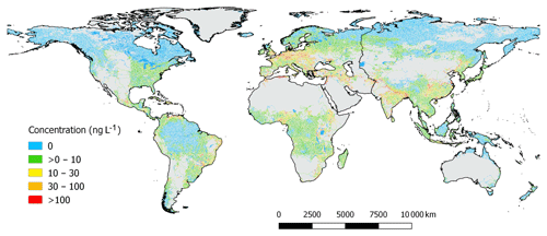
Model predictions were obtained with a run time of 5 min using a Desktop PC with Intel Core i5-4590 CPU 3.30 GHz and 8 GB RAM. The global concentration of diclofenac throughout the river network (Fig. 3) shows large areas of the world with a very low concentration of diclofenac (mainly in boreal and tropical latitudes), while densely populated areas, particularly in Europe, Asia, and Africa show very high concentrations, sometimes beyond 100 ng L⁻¹. Thresholds of diclofenac concentrations for the lowest observed effect on life concentration (LOEC, 30 ng L⁻¹) (Acuña et al., 2015) and the maximum acceptable limit proposed by the Water Framework Directive EC and the predicted non-effect concentrations (PNECs) (both at 100 ng L⁻¹, Grill et al., 2016) are crossed in large parts of the world (Fig. 3). Simulated concentrations of diclofenac above 100 ng L⁻¹ are detected in isolated areas of North America, several areas in Central America, and in some areas in South America. In Africa concentrations over the above thresholds occur in the western Mediterranean coast (Figs. 3 and 4), Nigeria, and eastern and south-east parts of the continent. Furthermore, certain areas in European countries show very high diclofenac concentrations, with remarkable prevalence in Belgium, central Europe, and Ukraine (Fig. 4). Concentrations over the thresholds are also found in western Asia. India and Bangladesh stand out, mainly in the Ganges basin. Several regions of China, Thailand, and Japan also show very high concentrations. Concentrations above 100 ng L⁻¹ are also observed in some Indonesian islands, such as Java.

Figure 3 Simulated mean annual diclofenac concentration worldwide.

The concentration maps in Figs. 3 and 4 do not show pixels with less than 100 mm yr⁻¹ of run-off, which correspond to arid regions. We decided to discard concentration values in these areas because the quality of the run-off product we used is very poor below this threshold (Fekete et al., 2002), so any result would be unreliable. In addition, we also identified unrealistic, huge diclofenac concentrations in large urban areas due to an unrealistic representation of river reaches and water infrastructure at our working resolution in these areas (sewage infrastructure in large urban areas is not accounted for in our model). To overcome this limitation, no diclofenac concentration is reported for cells accumulating contaminant mass for less than three upstream cells i.e. l<3 in Eq. (5). The two filters described above exemplify how the interpretation of GLOBAL-FATE outcomes depends on the available input datasets, both in terms of quality and resolution. Considering that working resolution and input datasets are user-dependent in GLOBAL-FATE, the criteria to assess model result quality and reliability are case dependent and the filters suggested here may not be convenient in all circumstances. In any case, users must be aware that the simplified representation of complex processes like water and contaminant routing along natural and engineered systems currently coded in GLOBAL-FATE implies serious limitations on the spatial scale at which the model delivers meaningful results (see Sect. 4 for a comprehensive discussion on this issue).

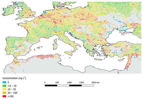
Figure 4 Simulated mean annual diclofenac concentration in central and southern Europe and the southern Mediterranean basin.

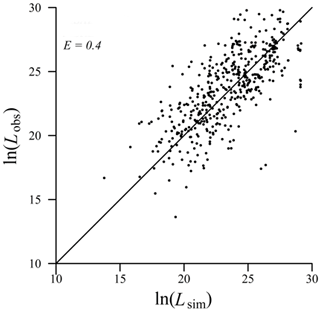
Although the aim of this exercise was only to exemplify the application of GLOBAL-FATE in a real case, we assessed the goodness of fit of model predictions against the observed loads of diclofenac in the river network. We used 405 diclofenac loading (concentration times streamflow) values measured in rivers around the globe compiled by Acuña et al. (2015), and we compared this with the modelled value in the corresponding cell after log-transforming the two values (the range of observed and modelled diclofenac loadings shows several orders of magnitude). We used the Nash–Sutcliffe model efficiency coefficient to assess model performance:

$$\begin{array}{}\text{(19)}& E=\mathrm{1}-{\displaystyle \frac{\sum {\left(L_{\mathrm{obs}}-L_{\mathrm{est}}\right)}^{\mathrm{2}}}{\sum {\left(L_{\mathrm{obs}}-\stackrel{\mathrm{‾}}{\left(\log L_{\mathrm{obs}}\right)}\right)}^{\mathrm{2}}}}.\end{array}$$

The relationship between observed and simulated diclofenac loads (Fig. 5) shows a Nash–Sutcliffe model efficiency of 0.4, which is reasonable considering that we did not calibrate any parameter of the model. Global models for contaminants always suffer from low to medium performance scores due to the scarce and spatially biased datasets available for model evaluation (Strokal et al., 2019), and frequently they only go beyond E>0.5 after intensive calibration procedures (e.g. Harrison et al., 2019).

Figure 5 Observed versus simulated-load log values (ln (ng∕L)); N=405 points. The Nash–Sutcliffe model efficiency coefficient (E) is also reported.

3.3 Sensitivity analysis

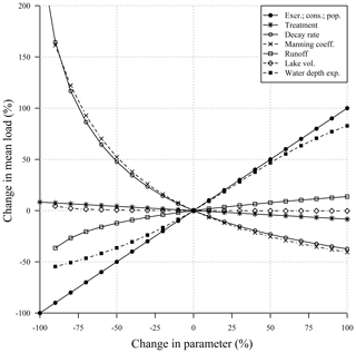
Model simulations may diverge from observed values due to uncertainty in observations and parametric values and to deliberate simplifications inherent in all phases of the modelling process. Furthermore, most input datasets come from previous modelling exercises with more assumptions and simplifications that may affect the final result. We carried out a sensitivity analysis in order to investigate the propagation of errors to the output from a selection of inputs (population, pharmaceutical consumption, excretion rate, run-off, decay rate in WWTPs and the river network, lake volume, Manning coefficient, and the d exponent in Eq. 11). This analysis was performed using a local sensitivity, one-at-a-time procedure, changing one input per simulation around a reference parametric point, defined by the values of the original datasets or the parametric value provided in Sect. 3.1. These inputs were perturbed around this reference point, decreasing and increasing the value from −100 % to 100 % of the original figure in 10 % increments. In the case of raster datasets, the whole domain was perturbed in a homogeneous way. We assessed the sensitivity of the mean diclofenac load in the river network to those perturbations in the inputs, expressed as percent change from the value in the reference condition.

The results from the sensitivity analysis (Fig. 6) suggest that the output of the model is highly sensitive to two groups of inputs. On the one hand, everything related to the generation of contaminant mass by population (population, consumption, and excretion rate) showed the largest overall sensitivity (the sensitivities are the same for these parameters because they multiply in the model; Eq. 14). On the other hand, the output was also very sensitive to parameters related to the attenuation of contaminant in the river network: the first-order decay rate in the river network and parameters related to water residence time calculation such as the Manning coefficient and the exponent d for water depth. The output showed less sensitivity to the rest of tested inputs. These results suggest that the quality of datasets related to the generation of contaminant from human use must be carefully checked and that the attenuation of the contaminants in rivers and lakes plays an important role in defining their presence in the river network. This last point is very relevant considering that data for first-order reaction rates in rivers for many contaminants are scarce or non-existent and that residence time calculation in the river network still depends on global empirical functions that may have large regional variability. Also, these results suggest that mitigation strategies to reduce the prevalence of pharmaceutical contaminants in the river network should point to increasing the assimilation of the drug by the human body and decisions and campaigns devoted to lower the per capita consumption. This would be much more efficient than increasing WWTP treatment technologies to attenuate the contaminant load before reaching the river network, at least in regions where the prevalence of waste water treatment is already high.

Figure 6 Spider plot of percent changes in the mean load in the river network due to changes in a collection of inputs to GLOBAL-FATE.

4 Strengths and limitations of GLOBAL-FATE

GLOBAL-FATE is an open-source, multiplatform, and modular contaminant-fate model that links human consumption of pharmaceutical-like compounds with their concentration in the river network. GLOBAL-FATE is also computationally efficient and can solve the whole global streamflow generation and contaminant routing in less than 5 min on a customary PC. It provides practical guidelines (through readme files and example datasets) to assist non-specialist users in computer programming. At the same time, it has a fully annotated code that experienced users can easily customize and further develop to adapt to their needs. The model is also available as a user-friendly QGIS plug-in. Through simple menus, an inexperienced user can conduct simulations and produce basic outputs on the QGIS canvas.

One of the features of GLOBAL-FATE is that it is not fundamentally associated with a spatial resolution or extent. Users can define the working spatial resolution and extent just by adapting the resolution of the raster inputs and the region of interest (for instance, a single continent or subcontinent). Although this is an obvious advantage over other large-scale contaminant models, it also harbours the significant risk that users may assume that the model delivers meaningful results at any working spatial scale. We strongly advise against the uncritical use of GLOBAL-FATE, particularly when working at coarse working resolutions or with highly spatially aggregated input data. We do not want to suggest a spatial resolution threshold from which results from GLOBAL-FATE could be regarded as reliable because the criteria to assess model results quality and reliability are case dependent, and guidelines suggested in a given situation may not be convenient in all circumstances. In our example, the combination of the working spatial scale (1∕16 of a degree, ∼7 km), the complexity of fine-scale interactions between engineered systems and the river network (e.g. the exact location of effluent discharges, extensive sewage networks, and poor representation of small streams), and the input data available translates into several model inadequacies that pose limits on the interpretation of the results. We have already mentioned that the quality of the run-off map precludes the interpretation of any results for regions where run-off is below 100 mm yr⁻¹ and that the calculated concentrations are unreliable for watersheds smaller than ∼150 km² (this roughly relates to river reaches of ∼20 km) due to inexact effluent discharge locations in small streams and the absence of data on sewage networks in large urban areas, which would route the contaminant load downstream towards larger rivers resulting in higher dilution and lower contaminant concentration. These limitations were easily spotted as they resulted in very unrealistic high diclofenac concentrations scattered throughout the global network, which attracted our immediate attention. However, other assumptions of the modelling approach do not leave such a conspicuous mark in the model output. For instance, consumption data are homogeneous at the country level, while variability in large countries may be substantial (urban vs. rural regions, for instance). Also, we have averaged information on the intensity of treatment at the country scale, although this may change even at very local scales. This implies that the model results are not necessarily unbiased beyond the threshold mentioned earlier (150 km²) because all uncertainties and biases propagating from model inputs and assumptions must also have a reflection in the spatial dimension at varying scales. For instance, the comparison between observed and modelled diclofenac concentrations along the main axis of the Rhine River (Fig. 7) shows that the model was able to spot a concentration increase at 300 km upstream of the river mouth (in the sense that the model predicts an increase that goes beyond 100 ng L⁻¹, the basic threshold we were interested in). However, in the same basin close to the river mouth (∼50 km) the model could not mimic an increase in concentration beyond 100 ng L⁻¹. Our opinion is that GLOBAL-FATE, as implemented in the example, should be used to answer questions which are general in nature, such as the question of whether, for example, contaminant concentration downstream from large urban areas in central Europe frequently exceeds 100 ng L⁻¹ and related statements concerning remediation measures. We advise against the use of GLOBAL-FATE as implemented in the example to support statements concerning particular places at or near the working resolution (for example, remediation measures seem insufficient to lower concentrations below 100 ng L⁻¹ downstream from Cologne). We acknowledge that this restriction limits the usability of the current version of GLOBAL-FATE to answer questions that require precise information at a scale of ∼20 km of river network. In such cases, models operating at local (i.e. single-watershed) or regional (i.e. country-level) scales may be a better option (e.g. Diamantini et al., 2019). Nevertheless, GLOBAL-FATE can be used to test the effectiveness of large-scale management strategies related to pharmaceutical consumption control and waste water treatment implementation and upgrading in order to deliver influential assessments of climate change impacts on pharmaceutical consumption and river network ecosystem health (e.g. the Inter-Sectoral Impact Model Intercomparison project) and also to inform global policy instruments like the UN Sustainable Development Goals agenda. This is already common practice in other sectors using large-scale, coarse-resolution models such as impacts of climate change on marine life (Lotze et al., 2019), on lake physics (Woolway and Merchant, 2019), on soil moisture (Samaniego et al., 2018), or on economic losses due to river flooding (Dottori et al., 2018), to cite just a few recent examples.

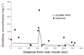
Figure 7 GLOBAL-FATE diclofenac simulation along the Rhine River (Europe) and diclofenac observations from our compiled database.

Nonetheless, we discussed the limitations of GLOBAL-FATE as applied in our example (∼7 km pixel resolution), but even exercises using models working at much finer resolution in smaller areas (e.g. China at 0.5 km resolution; Grill et al., 2018) found substantial uncertainties related to unaccounted for variability regarding input variables and poor representation of small streams. Therefore, we strongly suggest to carefully assess model performance irrespective of the working resolution and to pay special attention to the spatial scales at which answers are required. The questions must also be compatible with the aggregation of input information and the representation of the river network. Finally, GLOBAL-FATE includes very simplified physically based approximations for attenuation in the river network, which, a priori, are mathematically robust to changes in the spatial resolution but that assume homogeneous properties along calculation units (river reaches) such as water velocity and mixing. Although those assumptions do not hold even at very local scales (tens of metres), empirical research on river ecology suggests that this approach is reasonable for rivers reaches up to ∼10 km (Marcé et al., 2018). Beyond this, substantial heterogeneity of the river network is overlooked, with potential effects on the contaminant mass balance (Darracq and Destouni, 2007).

GLOBAL-FATE is a steady-state model, and although synoptic conditions like low to high flows or climate change scenarios can be modelled, it cannot dynamically simulate extreme events or seasonality. This should be considered when formulating research or management questions for which hydrological seasonal or subseasonal variability is relevant. An important aspect of GLOBAL-FATE is that researchers are free to use the input information they prefer; it is not limited to particular hydrological products, so synoptic conditions can always be modelled, as long as the steady-state assumption is reasonable.

GLOBAL-FATE is the first contaminant model operating at the global scale that fully integrates lakes and reservoirs in the routing of a contaminant along the river network. This is a relevant improvement over other modelling approaches, especially considering the long water residence time of lakes and reservoirs compared to river reaches, which implies a prominent role of lakes and reservoirs in the attenuation of contaminants. However, it should be noted that GLOBAL-FATE models lakes and reservoirs as point-like features, with no spatial heterogeneity. This may fail to capture likely gradients of contaminant concentration in large lakes and reservoirs.

Our analyses showed that GLOBAL-FATE will have a performance in terms of goodness of fit similar to other global contaminant-fate models. However, as in any other modelling exercise, this will be highly dependent on the quality of the input data used and the availability of observed data to adjust parameters that cannot be set at confident values using prior information. In any case, large uncertainties will always be present in global models including simplified lumped representations of very complex processes. We pointed to the main limitations of the model and the most sensitive inputs, but researchers will have to reassess these in a case-by-case fashion.

As to future developments, we envisage the inclusion of diffuse pollution in the current steady-state framework, which would make GLOBAL-FATE useful for a much wider range of pollutants, such as nutrients or agricultural pesticides, and a more detailed accounting of sewage infrastructure to be able to solve contaminant routing at high resolution in very large urban areas.