The Canadian Earth System Model version 5 (CanESM5.0.3)

The Canadian Earth System Model version 5 (CanESM5) is a global model developed to simulate historical climate change and variability, to make centennial-scale projections of future climate, and to produce initialized seasonal and decadal predictions. This paper describes the model components and their coupling, as well as various aspects of model development, including tuning, optimization, and a reproducibility strategy. We also document the stability of the model using a long control simulation, quantify the model's ability to reproduce large-scale features of the historical climate, and evaluate the response of the model to external forcing. CanESM5 is comprised of three-dimensional atmosphere (T63 spectral resolution equivalent roughly to 2.8^∘) and ocean (nominally 1^∘) general circulation models, a sea-ice model, a land surface scheme, and explicit land and ocean carbon cycle models. The model features relatively coarse resolution and high throughput, which facilitates the production of large ensembles. CanESM5 has a notably higher equilibrium climate sensitivity (5.6 K) than its predecessor, CanESM2 (3.7 K), which we briefly discuss, along with simulated changes over the historical period. CanESM5 simulations contribute to the Coupled Model Intercomparison Project phase 6 (CMIP6) and will be employed for climate science and service applications in Canada.

1 Introduction

A multitude of evidence shows that human influence is driving accelerating changes in the climate system, which are unprecedented in millennia (IPCC, 2013). As the impacts of climate change are increasingly being felt, so is the urgency to take action based on reliable scientific information (UNFCCC, 2015). To this end, the Canadian Centre for Climate Modelling and Analysis (CCCma) is engaged in an ongoing effort to improve modelling of the global Earth system, with the aim of enhancing our understanding of climate system function, variability, and historical changes, and making improved quantitative predictions and projections of future climate. The global coupled model, the Canadian Earth System Model (CanESM), forms the basis of the CCCma modelling system and shares components with the Canadian Regional Climate Model (CanRCM) for finer-scale modelling of the atmosphere (Scinocca et al., 2016), the Canadian Middle Atmosphere Model (CMAM) with atmospheric chemistry (Scinocca et al., 2008), and the Canadian Seasonal to Interseasonal Prediction System which is used for seasonal prediction and decadal forecasts (CanSIPS, Merryfield et al., 2013).

CanESM5 is the current version of CCCma's global model and has a pedigree extending back 40 years to the introduction of the first atmospheric general circulation model (GCM) developed at CCCma's predecessor, the Canadian Climate Centre (Boer and McFarlane, 1979; Boer et al., 1984; McFarlane et al., 1992). Successive versions of the model introduced a dynamic three-dimensional ocean in CGCM1 (Flato et al., 2000; Boer et al., 2000a, b), and later an interactive carbon cycle was included to form CanESM1 (Arora et al., 2009; Christian et al., 2010). The last major iteration of the model, CanESM2 (Arora et al., 2011), was used in the Coupled Model Intercomparison Project phase 5 (CMIP5) and continues to be employed for novel science applications such as generating large initial condition ensembles for detection and attribution (e.g. Kirchmeier-Young et al., 2017; Swart et al., 2018).

As detailed below, CanESM5 represents a major update to CanESM2. The leap from version 2 to version 5 was a one-off correction made to reconcile our internal model version labelling with the version label released to the public. The update includes incremental improvements to the atmosphere, land surface, and terrestrial ecosystem models. The major changes relative to CanESM2 are the implementation of completely new models for the ocean, sea ice, and marine ecosystems, and a new coupler. Model developers have a choice in distributing increasing, but finite, computational resources between improvements in model resolution, model complexity, and model throughput (i.e. number of years simulated). The resolution of CanESM5 (T63 or ∼ 2.8^∘ in the atmosphere and ∼ 1^∘ in the ocean) remains similar to CanESM2 and is at the lower end of the spectrum of CMIP6 models. The advantage of this coarse resolution is a relatively high model throughput given the complexity of the model, which enables many years of simulation to be achieved with available computational resources. The first major application of CanESM5 is CMIP6 (Eyring et al., 2016), and over 50 000 years of simulation are being conducted for the 20 CMIP6-endorsed model intercomparison projects (MIPs) in which CCCma is participating.

The aim of this paper is to provide a comprehensive reference that documents CanESM5. In the sections below, each of the model components is briefly described, and we also explain the approach used to develop, tune, and numerically optimize the model. Following that, we document the stability of the model in a long pre-industrial control simulation, and the model's ability to reproduce large-scale features of the climate system. Finally, we investigate the sensitivity of the model to external forcings.

2 Component models

In CanESM5, the atmosphere is represented by the Canadian Atmosphere Model (CanAM5), which incorporates the Canadian Land Surface Scheme (CLASS) and the Canadian Terrestrial Ecosystem Model (CTEM). The ocean is represented by a CCCma-customized version of the Nucleus for European Modelling of the Ocean model (NEMO), with ocean biogeochemistry represented by either the Canadian Model of Ocean Carbon (CMOC) in the standard model version labelled as CanESM5, or the Canadian Ocean Ecosystem model (CanOE) in versions labelled CanESM5-CanOE. The atmosphere and ocean components are coupled by means of the Canadian Coupler (CanCPL). Each of these components of CanESM5 are described further below.

2.1 The Canadian Atmospheric Model version 5 (CanAM5)

Version 5 of the Canadian Atmospheric Model (CanAM5) employs a spectral dynamical core with a hybrid sigma-pressure coordinate in the vertical. The package of physical parameterizations used by CanAM5 is based on an updated version of its predecessor, CanAM4 (von Salzen et al., 2013). The physics package includes a prognostic cloud microphysics scheme governing water vapour, cloud liquid water, and cloud ice; a statistical layer-cloud scheme; and independent cloud-base mass-flux schemes for both deep and shallow convection. Aerosols are parameterized using a prognostic scheme for bulk concentrations of natural and anthropogenic aerosols, including sulfate, black and organic carbon, sea salt, and mineral dust; parameterizations for emissions, transport, gas-phase and aqueous-phase chemistry; and dry and wet deposition account for interactions with simulated meteorology. CanAM5 employs a triangular truncation at total wavenumber 63 (T63) corresponding to an approximate isotropic resolution of 2.8^∘ in both latitude and longitude. In the vertical, 49 levels are employed with layer thicknesses that increase monotonically from approximately 100 m at the surface to 2 km at ∼ 1 hPa – the domain lid.

Updates to the package of physical parameterizations in CanAM5 over those in CanAM4 are as follows. While the radiative transfer solution in CanAM5 is similar to that in CanAM4, the representation of optical properties was improved through changes to the parameterization of albedos for bare soil, snow, and ocean whitecaps; cloud optics for ice clouds and polluted liquid clouds; improved aerosol optical properties and absorption by the water vapour continuum at solar wavelengths. For aerosols, the parameterization for emissions of mineral dust and dimethyl sulfide (DMS) was improved, while the bulk stratiform cloud microphysical scheme was modified to include a parameterization of the second indirect effect.

Parameterizations of surface processes were improved through an upgrade of the Canadian Land Surface Scheme (CLASS) from version 2.7 to 3.6.2 as well as the inclusion of a parameterization for subgrid lakes. CanESM5 represents the first coupled model produced by the CCCma in which the atmosphere and ocean do not employ coincident horizontal computational grids. As a consequence, CanAM5 was modified to support a fractional land mask, by generalizing its underlying surface to support grid-box fractional tiles of land and water. This tiling technology was extended to include land surface components of ocean, sea ice, and subgrid-scale lakes. In this way, appropriate fluxes can be provided to each component. A full description CanAM5 and its relation to CanAM4 will be provided in a companion paper in this special issue (Cole et al., 2019).

2.2 CLASS-CTEM

The CLASS-CTEM modelling framework consists of the Canadian Land Surface Scheme (CLASS) and the Canadian Terrestrial Ecosystem Model (CTEM) which together form the land component of CanESM5. CLASS and CTEM simulate the physical and biogeochemical land surface processes, respectively, and together they calculate fluxes of energy, water, CO₂, and wetland CH₄ emissions at the land–atmosphere boundary. The introduction of dynamic wetlands and their methane emissions is a new biogeochemical process added since the CanESM2 (but note that these methane emissions are strictly diagnostic, since atmospheric methane concentrations are specified).

CLASS is described in detail in Verseghy (1991, 2000) and Verseghy et al. (1993) and version 3.6.2 is used in CanESM5. It prognostically calculates the temperature for its soil layers, their liquid and frozen moisture contents, temperature of a single vegetation canopy layer if it is present as dictated by the specified land cover, and the snow water equivalent and temperature of a single snow layer if it is present. Three permeable soil layers are used with default thicknesses of 0.1, 0.25, and 3.75 m. The depth to bedrock is specified on the basis of the global dataset of Zobler (1986), which reduces the thicknesses of the permeable soil layers. CLASS performs energy and water balance calculations and all physical land surface processes for four plant functional types (PFTs) (needleleaf trees, broadleaf trees, crops, and grasses) and operates at the same subdaily time step as the rest of the atmospheric component.

CTEM models photosynthesis, autotrophic respiration from its three living vegetation components (leaves, stem, and roots), and heterotrophic respiration fluxes from its two dead carbon components (litter and soil carbon) and is described in detail in Arora (2003) and Arora and Boer (2003, 2005). CTEM's photosynthesis module operates within CLASS, at the same time step as rest of the atmospheric component. CTEM provides CLASS with dynamically simulated structural attributes of vegetation including leaf area index (LAI), vegetation height, rooting depth and distribution, and aboveground canopy mass, which change in response to changes in climate and atmospheric CO₂ concentration. All terrestrial ecosystem processes other than photosynthesis are modelled in CTEM at a daily time step. Terrestrial ecosystem processes in CTEM are modelled for nine PFTs that map directly to the PFTs used by CLASS. Needleleaf trees are divided into their deciduous and evergreen types, broadleaf trees are divided into cold and drought deciduous and evergreen types, and crops and grasses are divided into C₃ and C₄ versions based on their photosynthetic pathways. The reason for separation of PFTs for CTEM is the additional distinction that biogeochemical processes require. For example, the distinction between deciduous and evergreen versions of needleleaf trees is needed to simulate leaf phenology prognostically. Once leaf area index has been dynamically determined by CTEM, all CLASS needs to know is that this PFT is a needleleaf tree since the physics calculations do not require information about underlying deciduous or evergreen nature of leaves. Similarly, the C₃ and C₄ photosynthetic pathways of crops and grasses determine how they photosynthesize, thus affecting the calculated canopy resistance. However, once canopy resistance is known, CLASS does not need to know the underlying distinction between C₃ and C₄ crops and grasses to use this canopy resistance in its energy and water balance calculations.

While the modelled structural vegetation attributes respond to changes in climate and atmospheric CO₂ concentration, the fractional coverage of CTEM's nine PFTs is specified. A land cover dataset is generated based on a potential vegetation cover for 1850 upon which the 1850 crop cover is superimposed. From 1850 onwards, as the fractional area of C₃ and C₄ crops changes, the fractional coverage of the other non-crop PFTs is adjusted linearly in proportion to their existing coverage, as described in Arora and Boer (2010). The increase in crop area over the historical period is based on LUH2 v2h product (http://luh.umd.edu/data.shtml, last access: 1 October 2017) of the land use harmonization (LUH) effort produced for CMIP6 (Hurtt et al., 2011).

Both CanESM5 and its predecessor CanESM2 do not include nutrient limitation of photosynthesis on land since the terrestrial nitrogen cycle is not represented. However, both models include a representation of terrestrial photosynthesis downregulation based on Arora et al. (2009), who used results from plants grown in ambient and elevated CO₂ environments to emulate the effect of nutrient constraints. The tunable parameter determining the strength of this downregulation, and therefore the strength of the CO₂ fertilization effect, is higher in CanESM5 than in CanESM2, resulting in higher land carbon uptake in CanESM5. The tuning of this downregulation parameter value, used in CanESM5, is explained in Arora and Scinocca (2016) who evaluate several aspects of modelled historical carbon cycle against observation-based estimates. A land nitrogen cycle model for CTEM is currently being developed, which will make the photosynthesis downregulation parameterization obsolete in future versions of the model.

The calculation of wetland extent and methane emissions from wetlands is described in detail in Arora et al. (2018). In brief, dynamic wetland extent is based on the “flat” fraction in each grid cell with slopes less than 0.2 %. As the liquid soil moisture in the top soil layer increases above a specified threshold, the wetland fraction increases linearly up to a maximum value, equal to the flat fraction in a grid cell. The simulated CH₄ emissions from wetlands are calculated by scaling the heterotrophic respiration flux from the model's litter and soil carbon pools to account for the ratio of wetland-to-upland heterotrophic respiratory flux and the fact that some of the CH₄ flux is oxidized in the soil column before reaching the atmosphere.

Surface runoff and baseflow simulated by CLASS are routed through river networks. Major river basins are discretized at the resolution of the model and river routing is performed at the model resolution using the variable velocity river-routing scheme presented in Arora and Boer (1999). The delay in routing is caused by the time taken by runoff to travel over land in an assumed rectangular river channel and a groundwater component to which baseflow contributes. Streamflow (i.e. the routed runoff) contributes freshwater to the ocean grid cell where the land fraction of a CanAM grid cell first drops below 0.5 along the river network as the river approaches the ocean.

In CanESM5, glacier coverage is specified and static. Grid cells are specified as glaciers if the fraction of the grid cell covered by ice exceeds 40 %, based on the GLC2000 dataset (Bartholomé and Belward, 2005). The combination of this threshold and the model resolution results in glacier-covered cells predominantly representing the Antarctic and Greenland ice sheets, with a few glacier cells in the Himalayas, northern Canada, and Alaska. Snow can accumulate on glaciers, and any additional snow above the threshold of 100 kg m⁻² of snow water equivalent is converted into ice, and an equivalent mass of freshwater is immediately inserted into runoff – implicitly representing mass balance between accumulation and calving. Snow and ice on glaciers can be melted, with the water exceeding a ponding limit inserted into runoff. There is no explicit accounting for glacier mass balance or adjustment of glacier coverage. This represents a potentially infinite global source or sink of freshwater in the coupled system, particularly in climates which are far from the state represented by GLC2000. However, in practice, the timescales of our centennial-scale simulations are much shorter than the response times of ice sheet coverage, and any imbalances are small (Sect. 4).

2.3 NEMO modified for CanESM (CanNEMO)

The ocean component is based on NEMO version 3.4.1 (Madec and the NEMO team, 2012). It is configured on the tripolar ORCA1 C grid with 45 z-coordinate vertical levels, varying in thickness from ∼ 6 m near the surface to ∼ 250 m in the abyssal ocean. Bathymetry is represented with partial cells. The horizontal resolution is based on a 1^∘ Mercator grid, varying with the cosine of latitude, with a refinement of the meridional grid spacing to 1∕3^∘ near the Equator. The adopted model settings include the linear free surface formulation (see Madec and the NEMO team, 2012, and references therein). Momentum and tracers are mixed vertically using a turbulent kinetic energy scheme based on the model of Gaspar et al. (1990), implemented into NEMO physics by Blanke and Delecluse (1993). The tidally driven mixing in the abyssal ocean is accounted for following Simmons et al. (2004). Base values of vertical diffusivity and viscosity are $\mathrm{0.5}\times {\mathrm{10}}^{-\mathrm{5}}$ and $\mathrm{1.5}\times {\mathrm{10}}^{-\mathrm{4}}$ m² s⁻¹, respectively. A parameterization of double diffusive mixing (Merryfield et al., 1999) is also included. Lateral viscosity is parameterized by a horizontal Laplacian operator with an eddy viscosity coefficient of 1.0×10⁴ m² s⁻¹ in the tropics, decreasing with latitude as the grid spacing decreases. Tracers are advected using the total variance dissipation scheme (Zalesak, 1979). Lateral mixing of tracers (Redi, 1982) is parameterized by an isoneutral Laplacian operator with an eddy diffusivity coefficient of 1.0×10³ m² s⁻¹ at the Equator, which decreases poleward with the cosine of latitude. The process of potential energy extraction by baroclinic instability is represented with the Gent and McWilliams (1990) scheme using a spatially variable formulation for the mesoscale eddy transfer coefficient, as briefly described below.

Two modifications have been introduced to NEMO's mesoscale and small-scale mixing physics. The first modification is motivated by the observational evidence suggesting that away from the tropics the eddy scale decreases less rapidly than does the Rossby radius (e.g. Chelton et al., 2011). This is taken into consideration in the formulation for the eddy mixing length scale, which is used to compute the mesoscale eddy transfer coefficient for the Gent and McWilliams (1990) scheme (for details, see Saenko et al., 2018). The second modification is motivated by the observationally based estimates suggesting that a fraction of the mesoscale eddy energy could get scattered into high-wavenumber internal waves, the breaking of which results in enhanced diapycnal mixing (e.g. Marshall and Naveira Garabato, 2008; Sheen et al., 2014). A simple way to represent this process in an ocean general circulation model was proposed in Saenko et al. (2012). Here, we employ an updated version of their scheme which accounts better for the eddy-induced diapycnal mixing observed in the deep Southern Ocean (e.g. Sheen et al., 2014).

CanESM5 uses the LIM2 sea-ice model (Fichefet and Morales Maqueda, 1997; Bouillon et al., 2009), which is run within the NEMO framework. Some details regarding the calculation of surface temperature over sea ice are described in the coupling section below.

2.4 Ocean biogeochemistry

Two different ocean biogeochemical models, of differing complexity and expense, were developed in the NEMO framework: CMOC and CanOE. Two coupled models versions will be submitted to CMIP6. The version labelled as CanESM5 uses CMOC and was used to run all the experiments that CCCma has committed to. The version labelled CanESM5-CanOE, described in another paper in this special issue (Christian et al., 2019), is identical to CanESM5, except that CMOC was replaced with CanOE, and this version has been used to run a subset of the CMIP6 experiments, including DECK and historical (see Sect. 3.4). Both biogeochemical models simulate ocean carbon chemistry and abiotic chemical processes such as oxygen solubility identically, in accordance with the Ocean Model Intercomparison Project Biogeochemistry (OMIP-BGC) protocol (Orr et al., 2017).

2.4.1 Canadian Model of Ocean Carbon (CMOC)

The Canadian Model of Ocean Carbon was developed for earlier versions of CanESM (Zahariev et al., 2008; Christian et al., 2010; Arora et al., 2011) and includes carbon chemistry and biology. The biological component is a simple nutrient–phytoplankton–zooplankton–detritus (NPZD) model, with fixed Redfield stoichiometry, and simple parameterizations of iron limitation, nitrogen fixation, and export flux of calcium carbonate. CMOC was migrated into the NEMO modelling system, and the following important modifications were made: (i) oxygen was added as a passive tracer with no feedback on biology; (ii) carbon chemistry routines were updated to conform to the OMIP-BGC protocol (Orr et al., 2017); (iii) additional passive tracers requested by OMIP were added, including natural and abiotic dissolved inorganic carbon (DIC) as well as the inert tracers (CFC11, CFC12, and SF6).

2.4.2 Canadian Ocean Ecosystem Model (CanOE)

The Canadian Ocean Ecosystem Model (CanOE) is a new ocean biology model with a greater degree of complexity than CMOC and explicitly represents some processes that were highly parameterized in CMOC. CanOE has two size classes for each of phytoplankton, zooplankton, and detritus, with variable elemental (C ∕ N ∕ Fe) ratios in phytoplankton and fixed ratios for zooplankton and detritus. Each detritus pool has its own distinct sinking rate. In addition, there is an explicit detrital CaCO₃ variable, with its own sinking rate. Iron is explicitly modelled, with a dissolved iron state variable, sources from aeolian deposition and reducing sediments, and irreversible scavenging from the dissolved pool. N₂ fixation is parameterized similarly to CMOC with temperature and irradiance dependence and inhibition by dissolved inorganic nitrogen but no explicit N₂-fixer group. In addition, N₂ fixation is iron-limited in CanOE. In CanOE, denitrification is modelled prognostically and occurs only where dissolved oxygen is < 6 mmol m⁻³. Deposition of organic carbon is instantaneously remineralized at the sea floor as in CMOC, and CaCO₃ deposited at the sea floor dissolves if the calcite is undersaturated (whereas in CMOC, the burial fraction is implicitly 100 %). Carbon chemistry and all abiotic chemical processes such as oxygen solubility conform to the OMIP-BGC protocol (Orr et al., 2017) and are identical in CanOE and CMOC, except that in CMOC the carbon chemistry solver is applied only in the surface layer (as there is no feedback from saturation state to other biogeochemical processes in the subsurface layers). CanOE has roughly twice the computational expense of CMOC.

2.5 The Canadian Coupler (CanCPL)

CanCPL is a new coupler developed to facilitate communication between CanAM and CanNEMO. CanCPL depends on Earth System Modeling Framework (ESMF) library routines for regridding, time advancement, and other miscellaneous infrastructure (Theurich et al., 2016; Collins et al., 2005; Hill et al., 2004). It was designed for the multiple programme multiple data (MPMD) execution mode, with communication between the model components and the coupler via the Message Passing Interface (MPI).

The fields passed between the model components are summarized in Tables A1–A4. In general, CanNEMO passes instantaneous prognostic fields, which are remapped by CanCPL and given to CanAM as lower boundary conditions. These prognostic fields (sea-surface temperature, sea-ice concentration, and mass of sea ice and snow) are held constant in CanAM over the course of the coupling cycle. After integrating forward for a coupling cycle, CanAM passes back fluxes, averaged over the coupling interval, which are remapped in CanCPL and passed on to NEMO as surface boundary conditions. An exception is the ocean surface CO₂ flux, which is computed in CanNEMO and passed to CanAM. CanAM and CanNEMO are run in parallel, and the timing of exchanges through the coupler is indicated schematically in Fig. A1.

All regridding in CanCPL is done using the ESMF first-order conservative regridding option (ESMF, 2018), ensuring that global integrals remain constant for all quantities passed between component models (but see an exception below). The remapping weights w_ij, for a particular source cell i and destination cell j, are given by $w_{ij}=f_{ij}\times A_{{\text{s}}_i}/(A_{{\text{d}}_j}\times D_j)$, where f_ij is the fraction of the source cell i contributing to the destination cell j, $A_{{\text{s}}_i}$ and $A_{{\text{d}}_j}$ are the areas of the source and destination cells, and D_j is the fraction of the destination cell that intersects the unmasked source grid (ESMF, 2018).

Within the NEMO coupling interface, the “conservative” coupling option is employed. This option dictates that net fluxes are passed over the combined ocean–ice cell, and the fluxes over only the ice-covered fraction of the cell are also supplied, in principle allowing net conservation, even if the distribution of ice has changed given the unavoidable one coupling cycle lag encountered in parallel coupling mode. It was verified that the net heat fluxes passed from CanAM were identical to the net fluxes received by NEMO, to the level of machine precision. Conservation in the coupled model piControl run is discussed further in Sect. 4.

Sea-ice thermodynamics are computed in the LIM2 ice model, based on the surface fluxes received from CanAM and the basal heat flux from the NEMO liquid ocean. LIM2 provides the sea-ice concentration, snow and ice thickness to CanAM, via the coupler. The surface flux calculation in CanAM5 requires the ground temperature at the snow–sea-ice interface, GT_ice. The GT_ice for this purpose can be passed from LIM2 to CanAM once during each coupling cycle, or an alternative GT_ice can be evaluated in CanAM at every model time step, taking into account evolving surface albedo and atmospheric temperature (e.g. West et al., 2016). As implemented, when computing GT_ice, CanAM independently computes the conductive heat flux through sea ice, and there is no constraint that this flux, or GT_ice, is the same as that in LIM2. Conservation is maintained because the net heat flux between the atmosphere and sea ice is computed in CanAM and applied to LIM2, but different ice surface temperatures could result. Both approaches to computing surface fluxes were tested in CanESM5 and no major impacts on sea ice or the broader climate system relative to the default model were discovered. However, a significantly shorter coupling cycle of 1 h was required for convergence when fluxes were computed from the LIM2 GT_ice that was passed through the coupler. The shorter coupling period was required to more physically resolve the response to diurnal variations in radiative and sensible heat fluxes from the atmosphere (see, for example, West et al., 2016). The evaluation of fluxes from GT_ice computed in CanAM, on the other hand, was stable for coupling periods ranging from 1 to 24 h, with no major changes in the mean climate or variability immediately apparent. A final coupling cycle interval of 3 h was implemented for CanESM5 with the computation of fluxes based on the CanAM evaluation of GT_ice. These choices represented improved robustness and a compromise between greater efficiency (i.e. longer coupling periods) and maximum “realism”, which would be the 1 h coupling dictated by the length of the NEMO time step.

After a significant number of CMIP6 production simulations were complete, it was determined that while conservative remapping was desirable for heat and water fluxes, it introduced issues in the wind-stress field passed from CanAM to CanNEMO. Specifically, since CanAM is nominally 3 times coarser than CanNEMO, conservative remapping resulted in constant wind-stress fields over several NEMO grid cells, followed by an abrupt change at the edge of the next CanAM cell. This blockiness in the wind stress results in a non-smooth first derivative, and the resulting peaked wind-stress curl results in unphysical features in, for example, the ocean vertical velocities. Changing regridding of only wind stresses to the more typical bilinear interpolation, instead of conservative remapping, largely alleviates this issue. Sensitivity tests indicate no major impact on gross climate change characteristics such as transient climate response or equilibrium climate sensitivity, or on general features of the surface climate. However, there is an impact on local ocean dynamics, which led to the decision to submit a “perturbed” physics member to CMIP6. Hence, simulations submitted to CMIP6 labelled as perturbed physics member 1 (“p1”) use conservative remapping for wind stress, while those labelled as “p2” use bilinear regridding (see Sect. 3.4). A comparison between p1 and p2 runs is provided in Appendix E.

2.6 Treatment of greenhouse gases

CanESM5 represents radiative forcing from individual greenhouse gases (GHGs). Aside from CO₂, the concentrations of all radiatively active gases are specified and transiently evolve. Of these, CH₄, N₂O, and families of chlorofluorocarbons (CFCs) are assumed to be well mixed, while O₃ is specified as varying spatially – typically employing that prescribed for CMIP6 (Checa-Garcia et al., 2018). CanAM5 offers two modes for modelling CO₂ concentrations – as specified time-evolving concentrations or as a three-dimensional passive tracer driven by land–ocean surface emissions, prognostically derived through interactive coupling with biogeochemical carbon models in the land and ocean. For example, CanESM5 can be run with prognostic CO₂ in concert with specified anthropogenic fossil fuel emissions to simulate atmospheric CO₂ concentration through the historical and future periods. Wetland methane emissions simulated by CLASS-CTEM, in contrast, are purely diagnostic. While these emissions respond to changes in climate and atmospheric CO₂ concentration (through changes in vegetation productivity), they do not modify atmospheric CH₄ concentrations, which are specified.

3 Model development and deployment

3.1 Model tuning and spin up

Each of the CanESM5 component models (CanAM5, CLASS-CTEM, and CanNEMO) were initially developed independently, driven by observations in stand-alone configurations – CanAM5 in present-day (2003–2008) Atmospheric Model Intercomparison Project (AMIP) mode and CanNEMO in pre-industrial (PI) OMIP-like mode using CORE bulk formulae. In these configurations, free parameters were initially adjusted to reduce climatological biases assessed via a range of diagnostics. Further details of the CanAM5 tuning may be found in Cole et al. (2019). The component models were then brought together in a pre-industrial configuration (i.e. the piControl experiment), which was evaluated based on an array of diagnostics. Several thousand years of coupled simulation were run during the finalization of the model, and an approach was taken whereby AMIP simulations would be used to derive parameter adjustments in CanAM, which would then be applied to the coupled model.

Initial present-day configurations of CanAM5 that were tuned to give roughly the observed top-of-atmosphere net radiative forcing (top-of-atmosphere forcing ∼ 0.7–1.0 W m⁻²) in an AMIP simulation produced coupled piControl simulations that were too cold (global-mean near-surface temperatures below 12 ^∘C), with extensive sea ice and a collapsing meridional overturning circulation. One contributor to the tendency of the new coupled model to cool was the inclusion of the thermodynamic consequences of snowmelt in the open ocean, which induces an average global cooling of ∼ 0.5 W m⁻² in the piControl simulation, and was not included in the previous version, CanESM2.

This initial coupled-model cold bias was rectified by adjusting free parameters in CanAM, CLASS, and LIM2 in order to achieve a piControl simulation with a global-mean screen temperature of around 13.7 ^∘C (roughly the absolute value provided for 1850–1900 by the NASA-GISS, Berkeley Earth, and HadCRUT4 datasets) and a sea-ice volume within the spread of CMIP5 models, while maintaining a net top-of-atmosphere (TOA) radiative balance as close to 0 W m⁻² as possible. The specific parameters adjusted were emissivity of snow (from 1 to 0.97), snow grain size on sea ice, the drainage parameter controlling soil moisture, the LIM2 parameter controlling the lead closure rate (from 2.0 to 3.0), and most significantly the accretion rate in cloud microphysics. The accretion rate exerted the largest control, and sensitivity to this parameter is described more fully in a companion paper (Cole et al., 2019).

The consequence of the adjustments in CanAM5 was an increase in the present-day TOA forcing in AMIP mode from ∼ 1 to ∼ 2.5 W m⁻². Nonetheless, historical simulations of the coupled CanESM5 initialized from its equilibrated piControl show an increase in TOA forcing roughly matching the observed values of ∼ 0.7–1.0 W m⁻² over the 2003–2008 period for which CanAM5 was tuned in AMIP mode. The difference in patterns of sea surface temperature (SST) and sea-ice concentrations between the coupled model and observations is thought to be the cause of these differences in TOA balance between coupled and AMIP mode.

The final adjustment was to the carbon uptake over land so as to better match the observed value over the historical period, and achieved via the parameter which controls the strength of the CO₂ fertilization effect (Arora and Scinocca, 2016). No more extensive tuning of CanESM5 was undertaken. Critically, no tuning of climate sensitivity was undertaken – the transient and equilibrium climate sensitivity of CanESM5 are purely emergent properties. Once the tuned final configuration of CanESM5 was available, ocean potential temperature and salinity fields were initialized from World Ocean Atlas 2009, while CanAM, CLASS-CTEM, and CMOC were initialized from the restarts from earlier development runs. The model was spun up for over 1500 years prior to the launch of the official CMIP6 piControl simulation, which extends for a further 2000 years.

3.2 Code management, version control, and reproducibility

CanESM5 is the first version of the model to be publicly released, and this code sharing has been facilitated by the adoption of a new version-control-based strategy for code management. Additional goals of this new system are to adopt industry standard software development practices, to improve development efficiency, and to make all CanESM5 CMIP6 simulations fully repeatable.

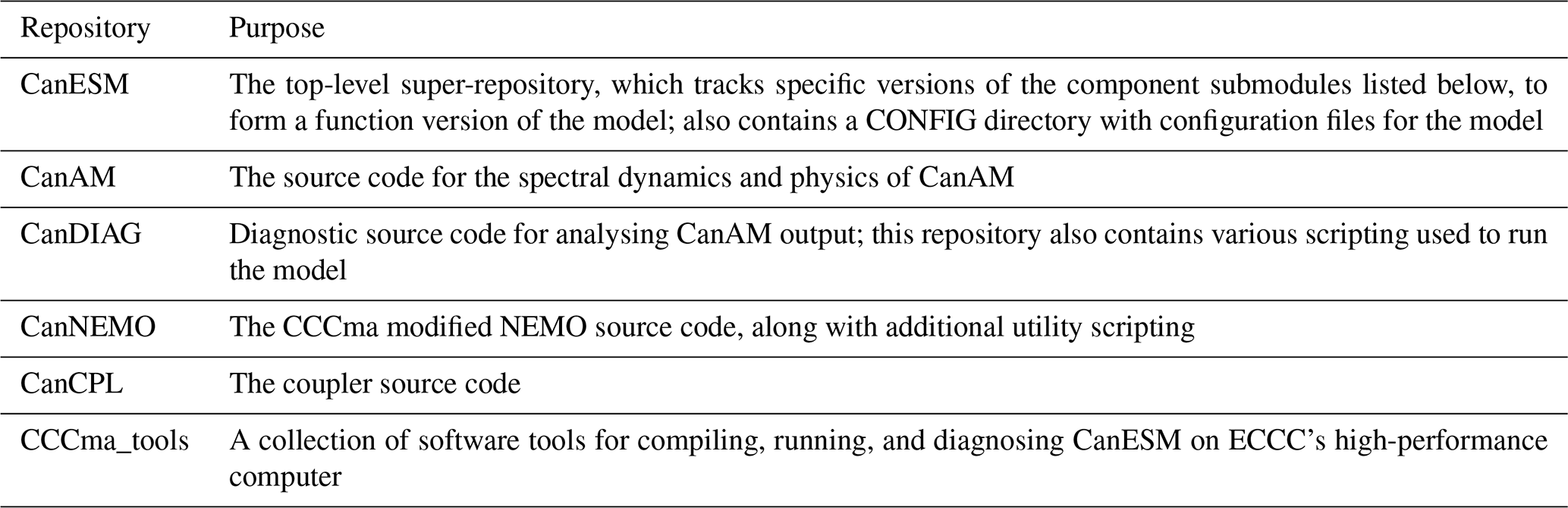
To maintain modularity, the code is organized such that each model component has a dedicated git repository for the version control of its source code (Table 1). A dedicated super-repository tracks each of the components as git submodules. In this way, the super-repo. keeps track of which specific versions of each component combine together to form a functional version of CanESM. A commit of the CanESM super-repo., which is representable by an eight-character truncated SHA1 checksum, hence uniquely defines a version of the full CanESM source code. The model development process follows an industry standard workflow (Table B1). New model features are merged onto the develop_canesm branch, which reflects the ongoing development of the model. Specific model versions, such as that used for CMIP6, are given tags and issued DOIs for ease of reference. We use an internal deployment of gitlab to host the model code and associated issue trackers, and we mirror the code to the public online code-hosting platform at https://gitlab.com/cccma/canesm (last access: 15 November 2019).

A dedicated ecosystem of software is used to configure, compile, run, and analyse CanESM simulations on Environment and Climate Change Canada (ECCC)'s high-performance computer (HPC) (Table B2). Several measures are taken to ensure modularity and repeatability. The source code for each run is recursively cloned from gitlab and is fully self contained. A strict checking routine ensures that any code changes are committed to the version control system and any run-specific configuration changes are captured in a dedicated configuration repository. A database records the SHA1 checksums of the particular model version and configuration used for every run, and these are included in CMIP6 NetCDF output for traceability. Input files for model initialization and forcing are also tracked for reproducibility (Table B1).

Table 1 Code structure and repositories.

Figure 1 Schematic of CanESM5 optimization. See Sect. 3.3 and Appendix C for details.

Our strategy of version control, run isolation, strict checking, and logging ensures that simulations can be repeated in the future, and the same climate will be obtained (bit-identical reproducibility is a further step and is dependant on machine architecture and compilers). The implementation of a clear branching workflow, and the uptake of modern tools such as issue trackers, and the gitlab online code-hosting application, has improved both collaboration and management of the code. This new system also led to large, unexpected improvements in model performance for two major reasons. The first was democratization of the code – via the promotion of group ownership of the code. The second was the freedom to experiment across the full code base ensured by our isolated run setup (Table B2), which was not possible under the previous system of using a single installed library of code shared across many runs. The performance gains achieved are described in the following section.

3.3 Model optimization and benchmarking

The ECCC HPC system consists of the following components: a “backend” Cray XC40, with two 18-core Broadwell CPUs per node (for 36 cores per node), and roughly 800 nodes in total, connected to a multi-PB lustre file system used as scratch space. This machine is networked to a “frontend” Cray CS5000, with several PB of attached spinning disk. This whole compute arrangement is replicated in a separate hall for redundancy, effectively doubling the available resources. Finally, a large tape-storage system (HPNLS) is available for archiving model results.

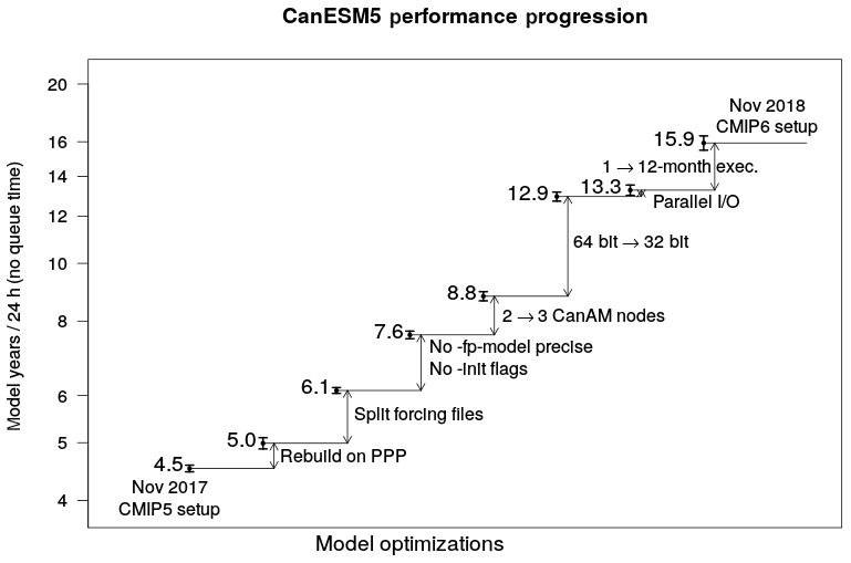
The initial implementation of a CanESM5 precursor on this new HPC occurred around 1 November 2017. The original workflow roughly followed that used for CanESM2 CMIP5 simulations. All CanESM5 components (atmosphere CanAM, coupler CanCPL, and ocean CanNEMO) were originally running at 64-bit precision. The atmospheric component CanAM was running on two 36-core compute nodes, the coupler was running on a separate node, and the ocean component was running on three nodes, resulting in six nodes in total. The initial throughput on the system, without queue time, was around 4.6 years of simulation per wall-clock day (ypd), or alternatively 0.02 simulation years per core day, when normalizing by the number of cores used.

In parallel to the physical model development, significant effort was made to improve the model throughput and eliminate a number of inefficiencies in the older CMIP5 workflow (Fig. 1). The largest effort was devoted to improving the efficiency of CanAM5, since this was identified as the major bottleneck. A brief summary of the improvements is given in Table C1 and Fig. 1. The most substantial and rewarding change was in converting the 64-bit CanAM component to 32-bit numerics. Since the remaining two components, CanCPL and CanNEMO, are still running at the 64-bit precision, the communication between CanAM and CanCPL required the promotion of a number of variables from 32-bit precision to 64-bit and back. The 32-bit CanAM implementation required a number of modifications to maintain the numerical stability of the code. Calculations in some subroutines, most notably in the radiation code, were promoted to the 64-bit accuracy. Conservation of some tracers, in particular CO₂, was compromised at the 32-bit precision, and some additional code changes to conserve CO₂ and maintain carbon budgets were implemented. Significant effort was also invested in optimizing compiler options used for NEMO to maximize efficiency, while the scalability of the NEMO code allowed sensibly increasing the node count to keep pace with the accelerated 32-bit version of CanAM.

In the final setup, the CanAM/CanCPL components are running on three shared compute nodes, and the ocean component CanNEMO is running on five nodes, resulting in eight nodes overall. The combined effect of the improvements listed in Table C1 resulted in more than tripling the original throughput to about 16 ypd (Fig. 1). Despite the increase in the total node count from six to eight, the efficiency of the model also improved roughly 3-fold, from 0.02 simulation years per core day of compute to about 0.06 years per core day. This final model configuration can complete a realization of the 165-year CMIP6 historical experiment in just over 10 d, compared to about 36 d, had no optimization been undertaken. At the time of writing, over 50 000 years of CMIP6 related simulation have been conducted with CanESM5, consuming about 1 million core days of compute time, resulting in about 8 PB of data archived to tape and over 100 TB of data publicly served on the Earth System Grid Federation (ESGF).

3.4 Model experiments and scientific application

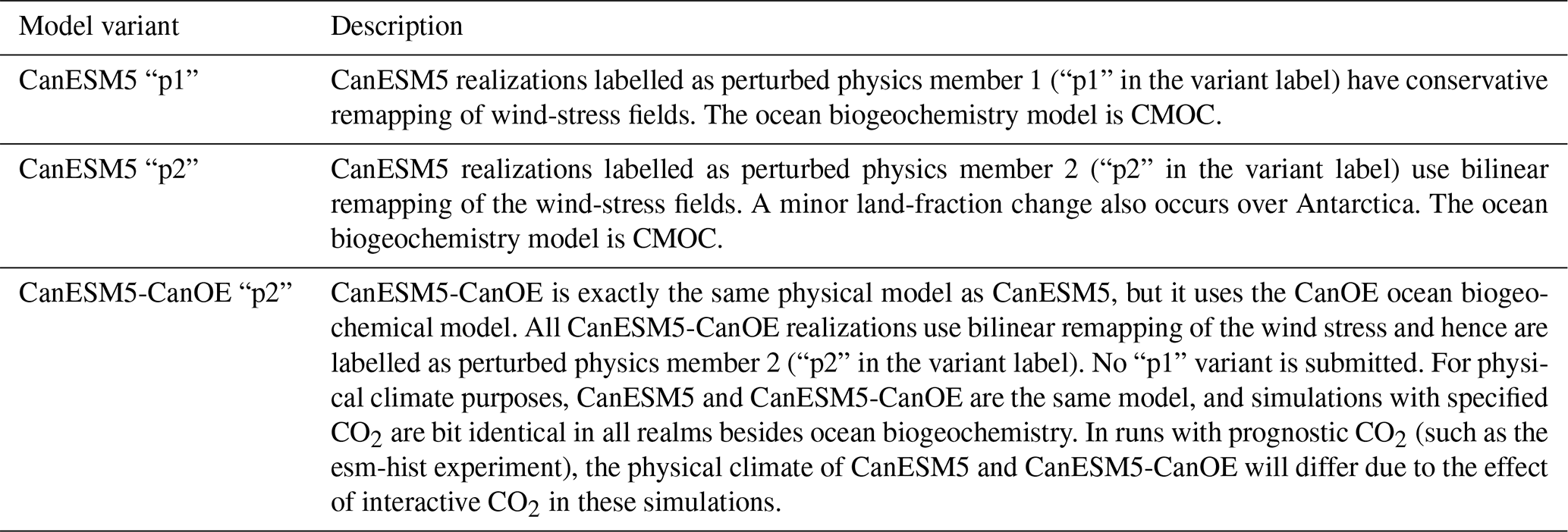
This section describes the major experiments and model variants of CanESM5 that are being conducted for the Coupled Model Intercomparison phase 6 (CMIP6), the first major science application of the model. Figure 2 shows the global-mean surface temperature for several of the key CMIP6 experiments, which can be used to infer important properties of the model, as discussed further in Sects. 4–6. Table 2 lists the variants of CanESM5 which are being submitted to CMIP6. These include the “p1” and “p2” perturbed physics members of CanESM5 (see Sect. 2.5) and a version of the model with a different ocean biogeochemistry model, CanESM5-CanOE.

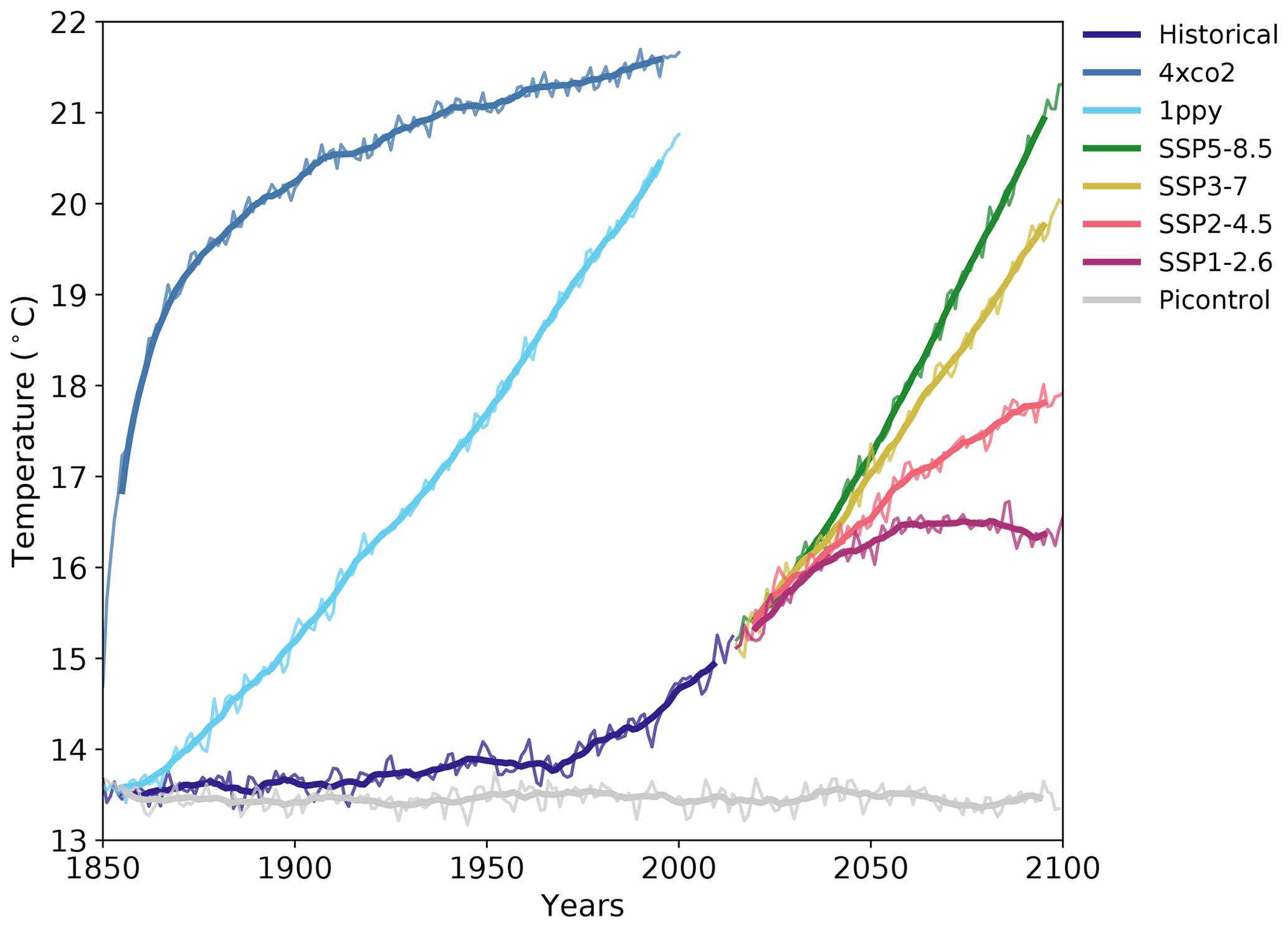
Figure 2 Global average screen temperature in CanESM5 for the CMIP6 DECK experiments, as well as the historical and tier 1 Shared Socioeconomic Pathway (SSP) experiments (SSP5-85, SSP3-70, SSP2-45, and SSP1-26). Thick lines are the 11-year running means; thin lines are annual means.

Table D1 lists the 20 CMIP6-endorsed MIPs in which CanESM5 is participating and which model variants are being run for each MIP. The volume of simulation continues to grow and will likely exceed 60 000 years. This is significantly more than the ∼ 40 000 years of CMIP6 simulation estimated by Eyring et al. (2016). The major reason for this is that significantly larger ensembles have been produced than formally requested. For example, CanESM5 will submit at least 25 realizations for the historical and tier 1 Shared Socioeconomic Pathway (SSP) experiments for each of the “p1” and “p2” model variants, for a total of 50 realizations, significantly more than the single requested realization. The scientific value of such large initial condition ensembles has become evident (e.g. Kay et al., 2015; Kirchmeier-Young et al., 2017; Swart et al., 2018) and motivates this approach.

Individual historical realizations (ensemble members) of CanESM5 were generated by launching historical runs at 50-year intervals off the piControl simulation. This is the same as the approach used to generate the five realizations of CanESM2, which were submitted to CMIP5. The 50-year separation was chosen to allow for differences in multi-decadal ocean variability between realizations. Below, we discuss the properties of the model, including illustrations of the internal variability generated spread across the historical ensemble. All results below are based on the CanESM5 p1 model variant.

Table 2 Model variants.

4 Stability of the pre-industrial control climate

The characteristics and stability of the CanESM5 pre-industrial control climate are evaluated using 1000 years of simulation from the CMIP6 piControl experiment, conducted under constant specified greenhouse gas concentrations and forcings for the year 1850 (Eyring et al., 2016). Ideally, a climate model and all its subcomponents would exhibit perfect conservation of tracer mass (e.g. water, carbon), energy, and momentum, and would be run for long enough to achieve equilibrium. In this case, we would expect to see, on a long-term average, zero net fluxes of heat, freshwater, and carbon at the interface between the atmosphere, ocean, and land surface, zero top-of-atmosphere net radiation, and constant long-term average temperatures or tracer mass within each component. In reality, however, models are not perfectly conservative due to the limitations of numerical representation (i.e. machine precision) as well as possible design flaws or bugs in the code, and models are generally not run to perfect equilibrium due to computational constraints. Despite imperfect conservation or spinup, models can still usefully be applied, as long as the drifts in the control run are small relative to the signal of interest, in our case historical anthropogenic climate. Below, we consider conservation and drift of heat, water, and carbon in CanESM5 (Fig. 3).

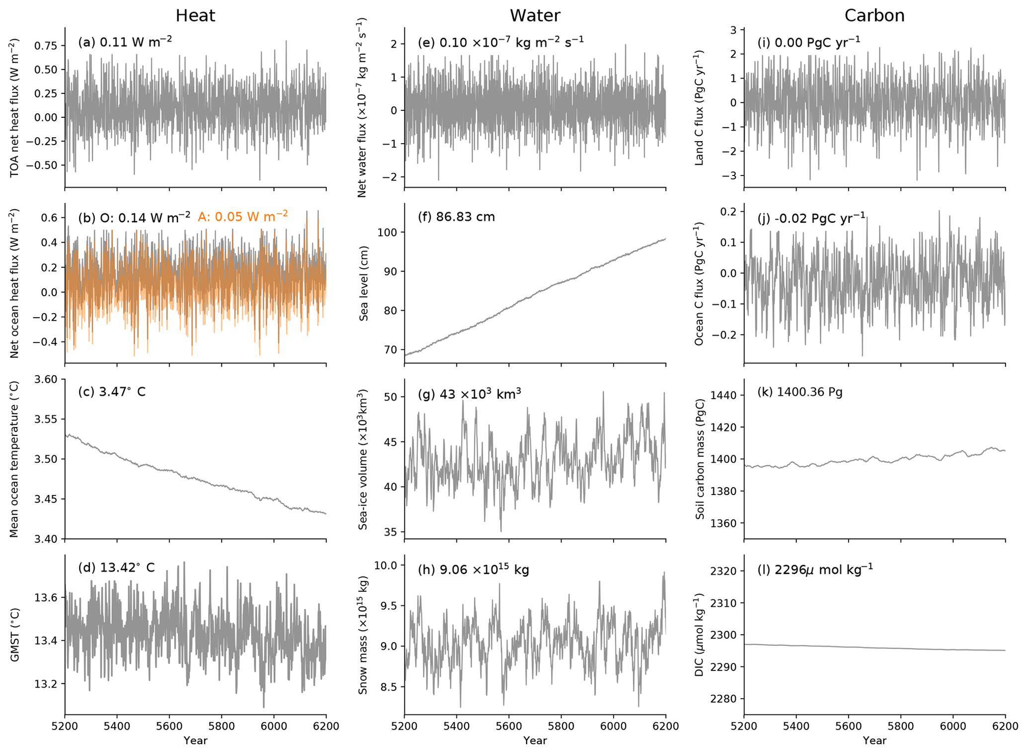
Figure 3 Stability of the CanESM5 piControl run showing global-mean (a) top-of-atmosphere net heat flux, (b) net heat flux at the surface of ocean; (c) volume-averaged ocean temperature; (d) screen temperature; (e) net freshwater input at the liquid ocean surface; (f) dynamic sea level; (g) sea-ice volume; (h) snow mass; (i) land–atmosphere carbon flux; (j) ocean–atmosphere carbon flux; (k) terrestrial soil carbon mass; and (l) ocean-dissolved inorganic carbon concentration. Inset numbers are the time average over the 1000 years shown. Heat fluxes in panels (a) and (b) are reported per metre squared of global area. The orange line in panel (b) is the heat flux computed at the bottom of the atmosphere, while the grey line is the heat flux computed at the surface of the liquid ocean (below sea ice).

The CanESM5 pre-industrial control shows a stable TOA net heat flux of 0.1 Wm⁻² (fluxes positive downward in m² of global area; Fig. 3a). The model is close to radiative equilibrium and this control net TOA heat flux is over an order of magnitude smaller than the signal expected from historical anthropogenic forcing (> 1 Wm⁻²). The global-mean screen temperature is stable at around 13.4 ^∘C (Fig. 3d), indicating thermal equilibrium, and approximately in line with estimates of the temperature in 1850. Half of the net TOA flux is passed from the atmosphere to the ocean (0.05 Wm⁻², Fig. 3b). With the conservative remapping in the coupler, the fluxes exchanged between components are identical to machine precision. However, the net heat flux received at the surface of the liquid ocean is 0.14 Wm⁻², almost 3 times higher than the heat flux passed from CanAM to NEMO (Fig. 3b). This discrepancy reflects a non-conservation of heat within the LIM2 ice model. Tests with an ice-free ocean do not suffer this problem. Nonetheless, the discrepancy is relatively small, and ice volume is stable. A further non-conservation occurs within the NEMO liquid ocean. Although the ocean receives a net heat flux of 0.14 Wm⁻², the volume-averaged ocean is cooling at a rate equivalent to a flux of 0.05 Wm⁻² (Fig. 3c), implying a total non-conservation of heat in the liquid ocean of about 0.2 Wm⁻². Conservation errors of this order are well known in NEMO v3.4.1, likely arise from the use of the linear free surface (Madec and the NEMO team, 2012), and have been seen in previous coupled models using NEMO (Hewitt et al., 2011). Despite this, the volume-averaged ocean temperature drift in CanESM5 is about half the size of the drift in CanESM2. Furthermore, the lack of ocean heat conservation in CanESM5 is roughly constant in time and appears to be independent of the climate (not shown).

At the liquid ocean surface, a small net freshwater flux results in a freshening trend and sea-level rise of about 24 cm over 1000 years (Fig. 3e, f). This rate of drift is more than 20 times smaller than the signal of anthropogenic sea-level rise. The LIM2 ice model appears to be the source of non-conservation: the net freshwater flux provided from CanAM is very close to zero, about 6 times smaller than that noted above (24 cm per 1000 years). Snow and ice volume are stable, not exhibiting any long-term drift, yet they are subject to considerable decadal- and centennial-scale variability (Fig. 3g, h).

Atmosphere–land carbon fluxes average to zero, and carbon pools within CTEM are stable (Fig. 3i, k). The net ocean carbon flux is fairly close to zero but remains slightly negative on average at −0.02 Pg yr⁻¹ despite a multi-millennial spinup (Fig. 3j). The total mass of dissolved inorganic carbon in the ocean decreases very slightly as a result (Fig. 3l). The rate of ocean carbon drift is approximately an order of magnitude smaller than the modern-day anthropogenic signal of ocean carbon uptake (> 2 Pg yr⁻¹). The drifts identified above are all far smaller than would be expected from anthropogenically forced trends, confirming that the model is suitably stable to evaluate centennial-scale climate change. In the following section, we consider the ability of the model to reproduce large-scale features of the observed historical climate.

5 Evaluation of historical-mean climate

In this section, we use the CMIP6 historical simulations (Eyring et al., 2016) of CanESM5 “p1”, focusing on climatologies computed over 1981 to 2010, unless otherwise noted.

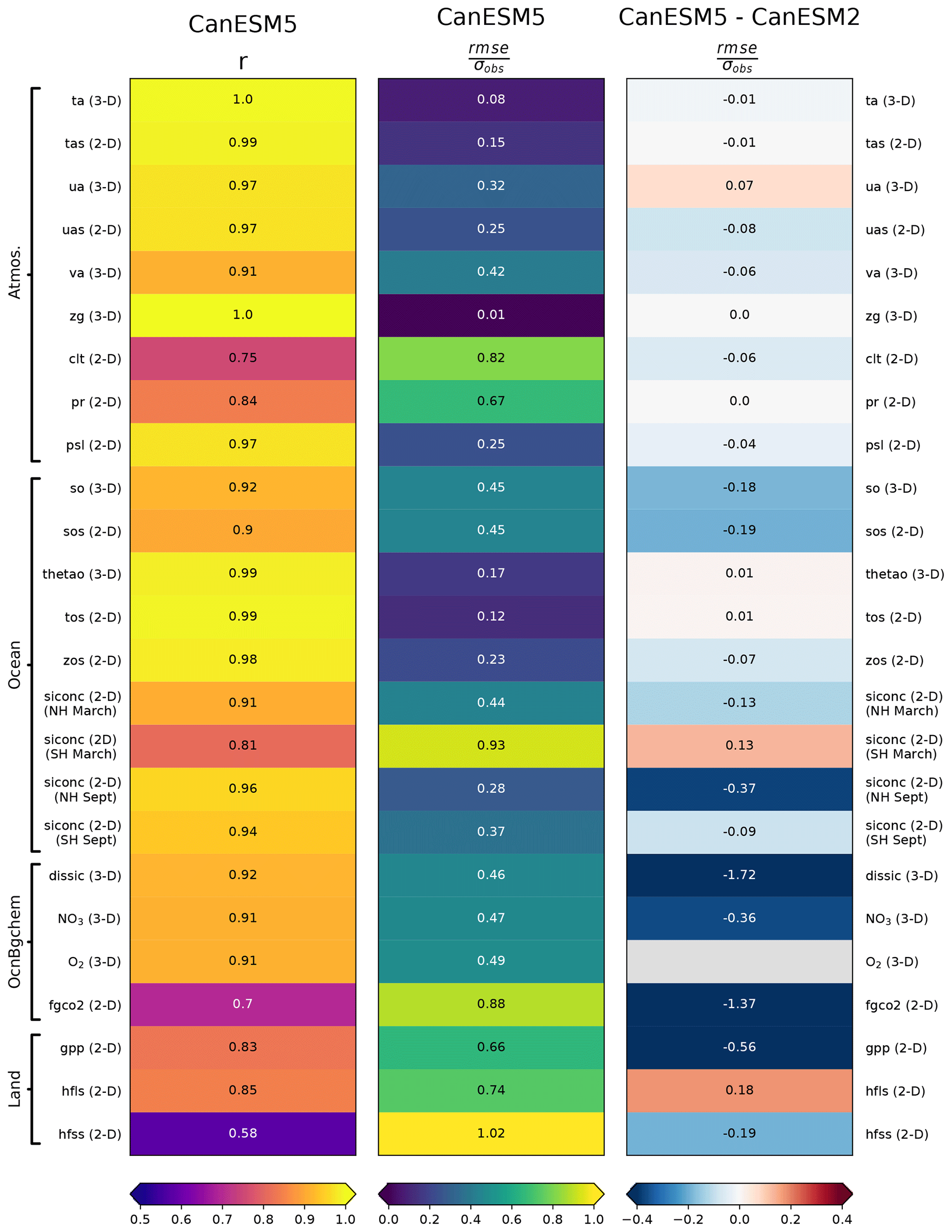
Figure 4 Summary statistics quantifying the ability of CanESM to reproduce large-scale climate features. Shown are the correlation coefficient (r) between the simulated and observed spatial patterns, the root mean square error (RMSE) normalized by the (observed spatial) standard deviation (σ), and the difference in normalized RMSE between CanESM5 and CanESM2. The spatial quantities represent temporal means over 1981 to 2010, except as noted in Appendix F. Variables are labelled according to the names in the CMIP6 data request and are defined in Table F3.

5.1 Overall skill measures

The ability of CanESM5 to reproduce observed large-scale spatial patterns in the climate system is quantified using global summary statistics computed over the 1981 to 2010 mean climate (Fig. 4). Shown are the correlation coefficient between CanESM5 and observations (r), the root mean square error (RMSE) normalized by the observed (spatial) standard deviation (σ), and the change in normalized RMSE between CanESM2 and CanESM5. The statistics are weighted by grid cell area for 2-D fields and volume for 3-D ocean fields, and by area and pressure for 3-D atmospheric variables. In general, CanESM5 successfully reproduces many observed spatial patterns of the surface climate, interior ocean, and the atmosphere, with correlation coefficients between the model and observations generally above 0.8. Some exceptions are the total cloud fraction (clt, r=0.75), atmosphere–ocean CO₂ flux (fgco2, r=0.7), and the surface sensible heat flux (hfss, r=0.58).

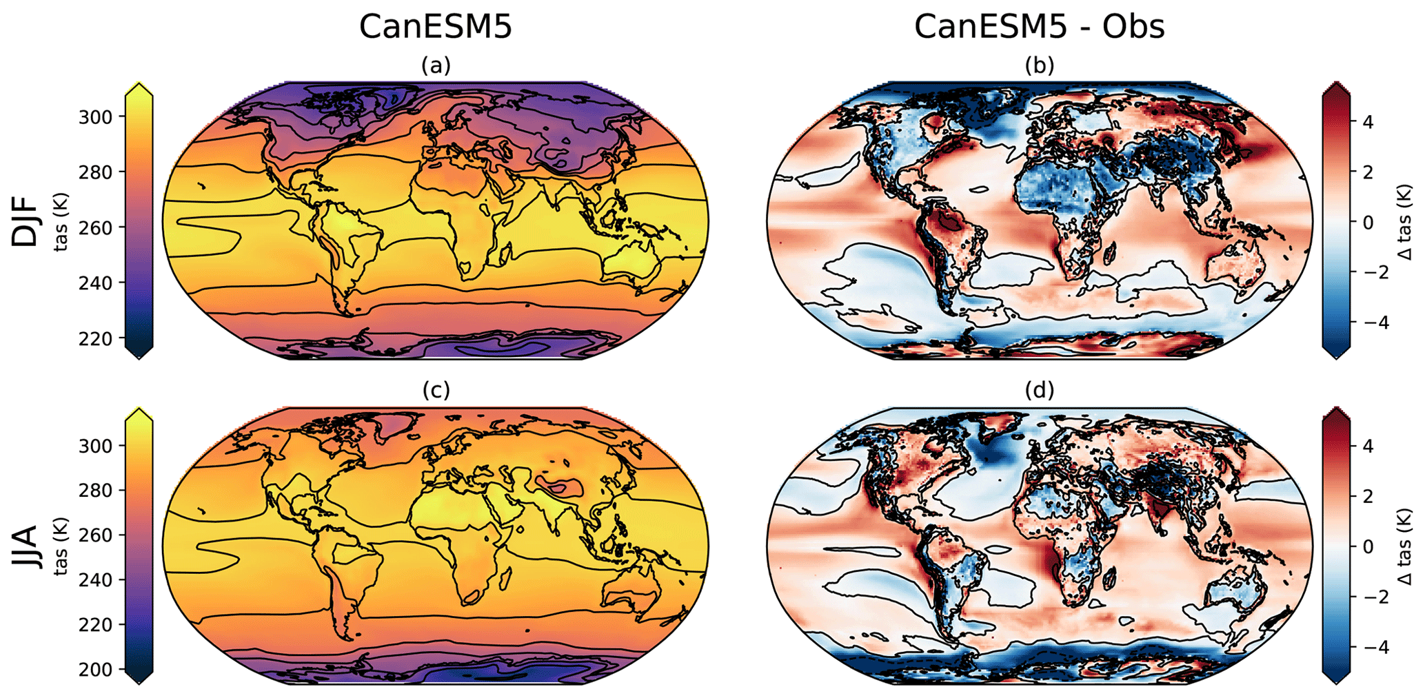
Figure 5 Climatologies of surface air temperature over 1981 to 2010 in CanESM5 (a, c) and their bias from ERA5 over the same period (b, d) shown for the DJF (a, b) and JJA (c, d) seasons.

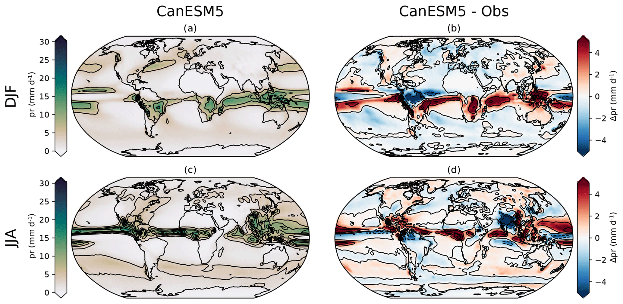
Figure 6 Climatologies of precipitation over 1981 to 2010 in CanESM5 (a, c) and their bias from the Global Precipitation Climatology Project (GPCP) over the same period (b, d) shown for the DJF (a, b) and JJA (c, d) seasons.

For most variables, normalized RMSE has decreased in CanESM5 relative to CanESM2, indicating an improvement in the ability of the new model to reproduce observed climate patterns over its predecessor. The largest improvements were seen for ocean biogeochemistry variables, while small increases in error were seen for 3-D distribution of zonal winds (ua), sea-surface temperatures (tos), the March distribution of sea ice in the Southern Hemisphere (siconc), and surface latent heat flux (hfls). In the following sections, individual realms are examined, with a closer look at regional details and biases.

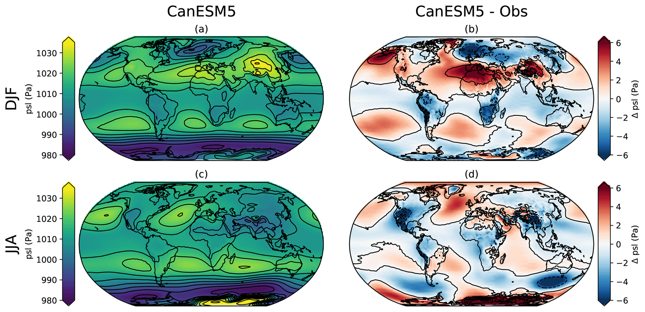
Figure 7 Climatologies of sea-level pressure over 1981 to 2010 in CanESM5 (a, c) and their bias from ERA5 over the same period (b, d) shown for the DJF (a, b) and JJA (c, d) seasons.

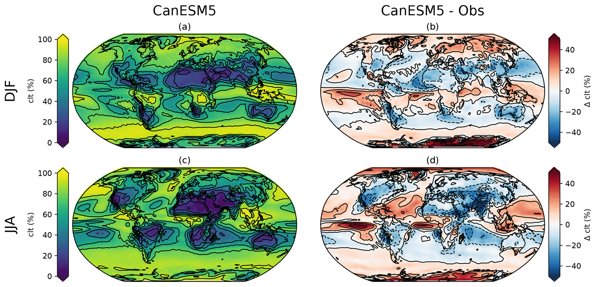
Figure 8 Cloud fraction in CanESM5 (a, c) and their bias with respect to International Satellite Cloud Climatology Project H series (ISCCP-H) satellite-based observations (b, d) shown for the DJF (a, b) and JJA (c, d) seasons.

5.2 Atmosphere

CanESM5 reproduces the large-scale climatological features of surface air temperatures (Fig. 5), precipitation (Fig. 6), and sea-level pressure (Fig. 7), though significant regional biases exist. CanESM5 is significantly colder than observed over sea-ice-covered regions (Fig. 5), noticeable in the Southern Ocean and in the region surrounding the Labrador Sea, which has extensive seasonal sea-ice cover in CanESM5 (see below). The Tibetan Plateau, the Sahara, and the broader North Atlantic Ocean are also cooler than observed. Warm biases exist over the eastern boundary current systems (Benguela, Humboldt, and California) and over the Amazon, eastern North America, much of Siberia, and broad regions of the tropical and subtropical oceans.

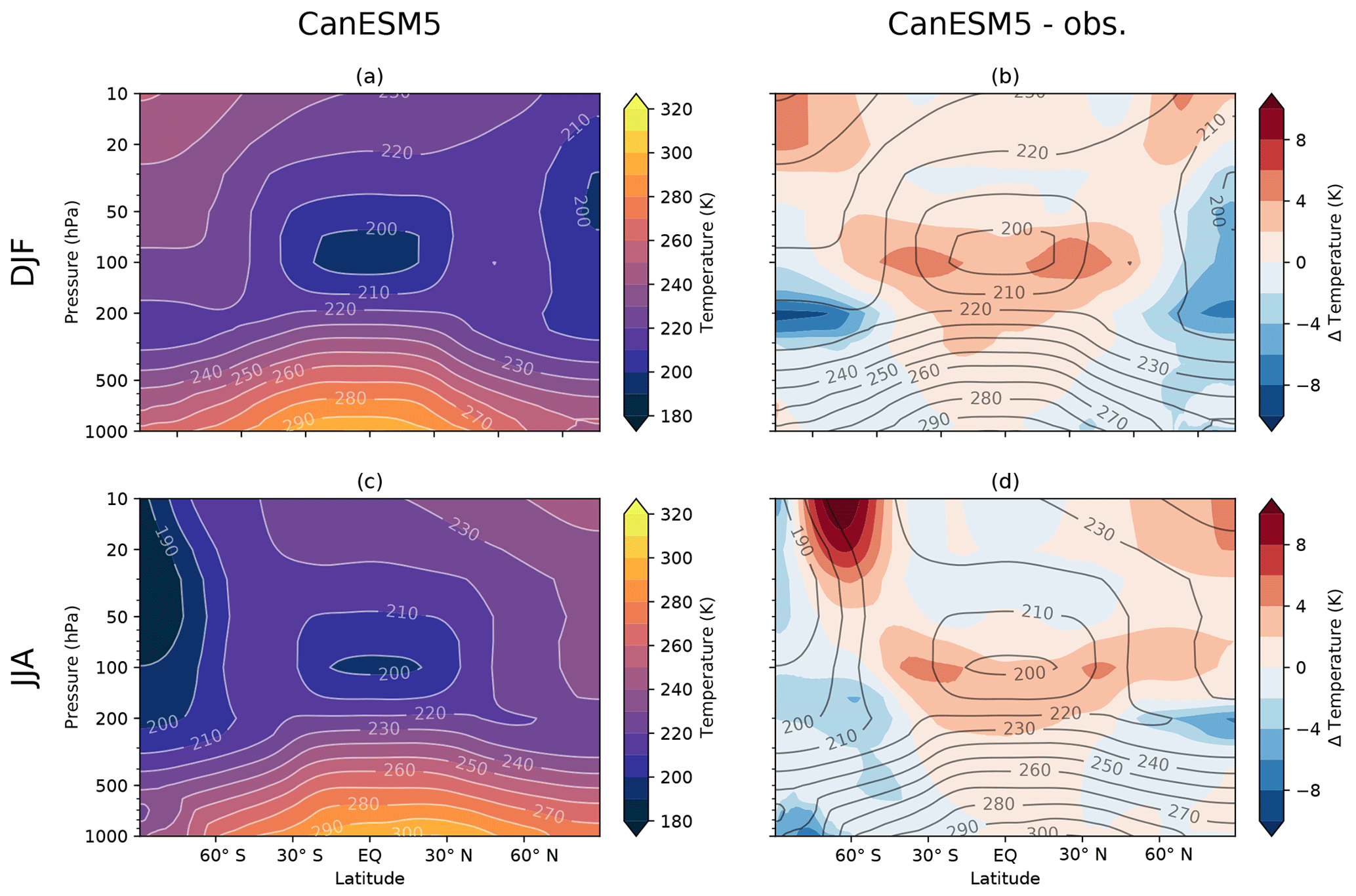
Figure 9 Zonal-mean temperature in CanESM5 (a, c) and bias relative to ERA5 (b, d) over 1981–2010 for the DJF (a, b) and JJA (c, d) seasons.

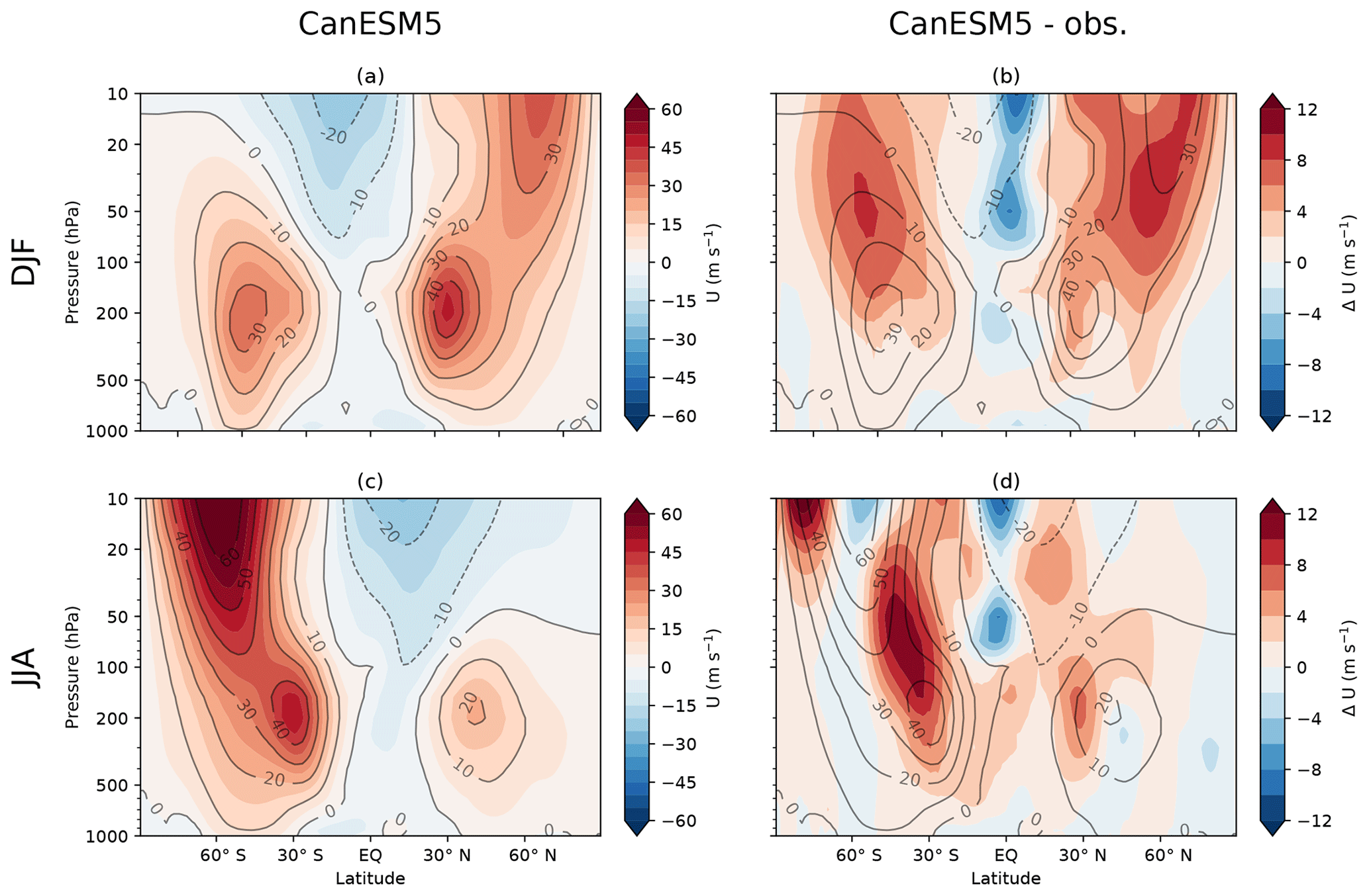
Figure 10 Zonal-mean zonal winds (a, c) and bias relative to ERA5 (b, d) over 1981–2010 for the DJF (a, b) and JJA (c, d) seasons.

Precipitation biases vary in sign by region (Fig. 6). The largest biases are over the tropical Pacific and Atlantic oceans, between the Equator and extending into the southern subtropics. The overall pattern of precipitation biases is very similar to that seen across the CMIP5 (Flato et al., 2013) and CMIP3 (Lin, 2007) models. The largest land biases are excessive precipitation over much of sub-Saharan Africa, southeast Asia, Canada, and Peru–Chile. In contrast, western Asia, Europe, the North Atlantic, and the subtropical to high-latitude Southern Ocean have too little simulated precipitation. The large-scale pattern of sea-level pressure is captured by CanESM5 (Fig. 7). Biases relative to ERA5 are largest over the high elevations of Antarctica (Fig. 7), possibly reflecting differences in the extrapolation of surface pressure to sea level.

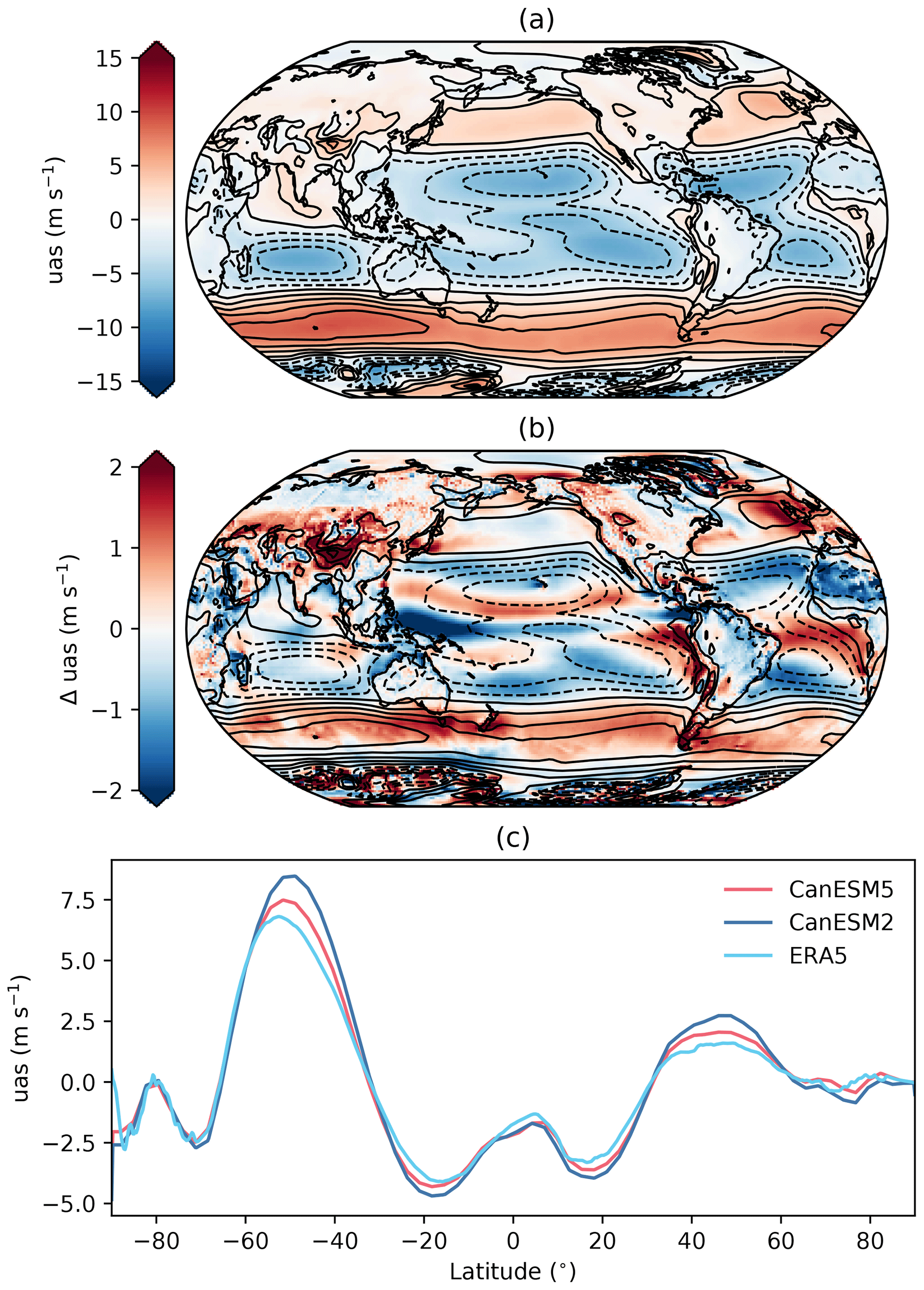
Figure 11 (a) Zonal surface winds in CanESM5, (b) the bias relative to ERA5, and (c) zonal-mean zonal surface winds in CanESM2, CanESM5, and ERA5.

Relative to ISCCP-H (Young et al., 2018) version 1.00 (Rossow et al., 2016), the total cloud fraction in CanESM5 is overestimated along the Equator, particularly in the eastern tropical Pacific and Atlantic (Fig. 8). A too-large cloud fraction is also found over Antarctica and the Arctic. Underestimations of total cloud fraction occur over most other land areas, with the largest underestimations over Asia and the Himalayas.

Zonal-mean sections of air temperature for the DJF and JJA seasonal means are shown in Fig. 9. In both seasons, CanESM5 is biased warm relative to ERA5 near the tropopause, across the tropics and subtropics. Warm biases also occur in the stratosphere, notably near 60^∘ S above 50 hPa in JJA. Cold biases exist from the subtropics to the high latitudes, where they reach from the surface to the stratosphere, and are strongest in the winter season.

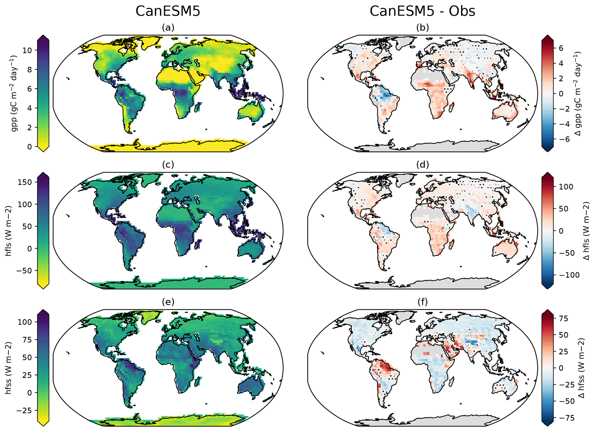
Figure 12 Time-mean values of (a) gross primary productivity (GPP), (c) latent heat flux (hfls), and (e) sensible heat flux (hfss) from CanESM5 (r1i1p1f1) (a, c, e) and the corresponding biases with respect to observation-based reference data presented in Jung et al. (2009) (b, d, f). Black dots mark grid cells where biases are not statistically significant at the 5 % level using the two-sample Wilcoxon test.

Figure 13 Zonal-mean values of (a) GPP, (b) HFLS, and (c) HFSS for CanESM5 (r1i1p1f1) and reference data from Jung et al. (2009). The shading presents the corresponding interquartile range that results from interannual variability as well as longitudinal variability for the period 1982 to 2008.

Zonal-mean zonal winds are compared to ERA5 in Fig. 10 for DJF and JJA. The westerly jets in CanESM5 are biased strong, particularly aloft, and in the winter hemisphere. Surface zonal winds in CanESM5 are only slightly stronger than observed and are significantly improved over those in CanESM2 (Fig. 11), which were too strong, particularly over the Southern Hemisphere westerly jet.

5.3 Land physics and biogeochemistry

Figures 12 and 13 compare the geographical distribution and zonal averages of gross primary productivity (GPP) and latent and sensible heat fluxes over land with observation-based estimates from Jung et al. (2009). The zonal averages of GPP, and latent and sensible heat fluxes compare reasonably well with observation-based estimates, although the latent heat fluxes are somewhat higher especially in the Southern Hemisphere, as discussed below (Fig. 13). Figure 12 shows the biases in the simulated geographical distribution of these quantities. In the tropics, biases in GPP, and latent and sensible heat fluxes broadly correspond to biases in simulated precipitation compared to observation-based estimates (shown in Fig. 6).

Generally over the tropics, as would be intuitively expected, the signs of GPP and latent heat flux anomalies are the same since they are both affected by precipitation in the same way. Sensible heat flux is expected to behave in the opposite way compared to GPP and latent heat flux in response to precipitation biases. For example, simulated GPP and latent heat fluxes are lower, and sensible heat fluxes higher in the northeastern Amazonian region because simulated precipitation is biased low (Fig. 6). The opposite is true for almost the entire African region south of the Sahara and most of Australia. Here, simulated precipitation that is biased high, compared to observations, results in simulated GPP and latent heat flux that are higher and sensible heat flux that is lower than observation-based estimates. At higher latitudes, where GPP and latent heat flux are limited by temperature and available energy, the biases in precipitation do not translate directly into biases in GPP and latent heat flux as they do in the tropics.

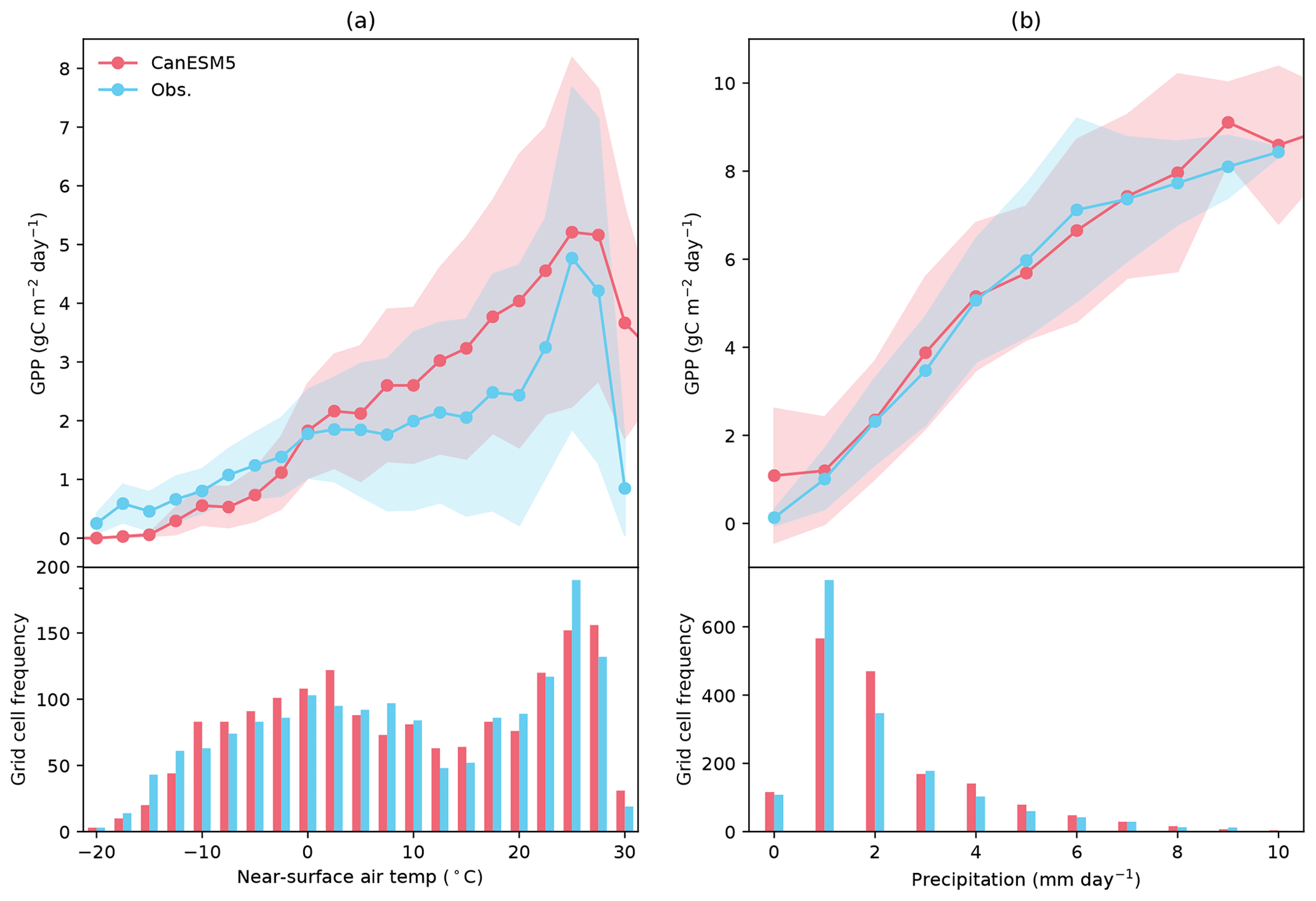
Figure 14 Functional response of GPP to (a) near-surface air temperature and (b) surface precipitation for CanESM5 (r1i1p1f1) and reference data from Jung et al. (2009). Values present monthly mean values averaged over the period 1982 to 2008 and the shading shows the corresponding standard deviation.

The biases in simulated climate imply that simulated land surface quantities will also be biased, which makes it difficult to assess if the underlying model behaviour is realistic. This limitation can be alleviated to some extent by looking at the functional relationships between a quantity and its primary climate drivers. This technique works best when a land component is driven offline with meteorological data. In a coupled model, as is the case here, land–atmosphere feedbacks can potentially worsen a model's performance by exaggerating an initial bias. For example, low model precipitation can be further reduced due to feedbacks from reduced evapotranspiration, some of which is recycled back into precipitation. Figure 14 shows the functional relationships between GPP and temperature, and GPP and precipitation, for both model- and observation-based estimates. The observation-based temperature and precipitation data used in these plots are from CRU-JRA reanalysis data that were used to drive terrestrial ecosystem models in the TRENDY intercomparison for the 2018 Global Carbon Budget (Le Quéré et al., 2018). Figure 14 shows that GPP increases both with increases in precipitation (as would be normally expected) and temperature except at mean annual values above 25 ^∘C when soil moisture limits any further increases. This threshold emerges both in the model- and the observation-based functional relationships. With the caveat mentioned above, the functional relationships of GPP with temperature and precipitation based on simulated data compare reasonably well with those based on observation data, although the simulated GPP relationship with precipitation compares much better to its observation-based relationship than that for temperature.

As mentioned earlier, dynamically simulated wetland extent and wetland methane emissions in CanESM5 are purely diagnostic. Figure G1 in Appendix G compares zonal distribution of simulated annual maximum wetland extent with observation-based estimates and shows the temporal evolution of annual maximum wetland extent and wetland methane emissions over the historical period.

5.4 Physical ocean

CanESM5 reproduces the observed large-scale features of sea-surface temperature (SST), salinity (SSS), and height (SSH) (Fig. 15). The largest SST biases are the cold anomalies southeast of Greenland and in the Labrador Sea (Fig. 15b). These negative SST biases are associated with excessive sea-ice cover, described further below, and with the surface air temperature biases mentioned above. Positive SST biases are largest in the eastern boundary current upwelling systems, as for surface air temperatures.

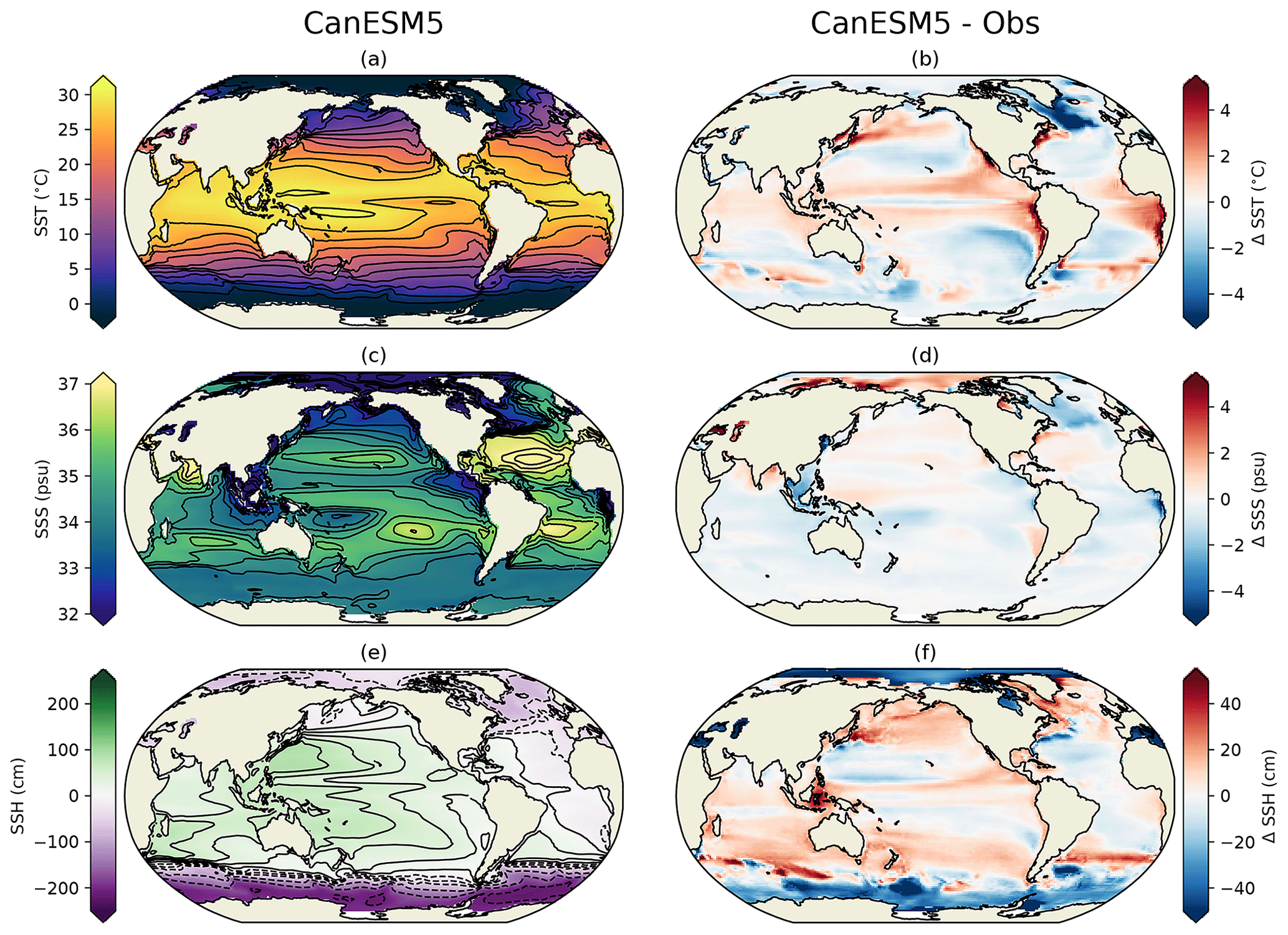
Figure 15 Sea-surface (a) temperature, (c) salinity, and (e) height averaged over 1981 to 2010, their biases relative to World Ocean Atlas 2009 (b, d), and the Aviso mean dynamic topography (f).

Figure 16 CanESM5 zonal-mean ocean (a) potential temperature, (c) salinity averaged over 1981 to 2010, and their biases from World Ocean Atlas 2009 (b, d). Note that the depth scale on the y axis is non-uniform.

Figure 17 CanESM5 residual meridional overturning circulation in the Atlantic (a), Indo-Pacific (b), and global (c) oceans, averaged over 1981 to 2010, including all resolved and parameterized advective processes. Note that the depth scale on the y axis is non-uniform.

Sea-surface salinity biases are largest, and positive, around the Arctic coastline, potentially indicating insufficient runoff in this region (Fig. 15d). Negative annual-mean SSS biases occur in the Labrador Sea and are also found in seas of the maritime continent and eastern tropical Atlantic. SSH is shown as an anomaly from the (arbitrary) global mean (Fig. 15e). Significant SSH biases are associated with the positions of western boundary currents, noticeably for the Gulf Stream and Kuroshio Current (Fig. 15f). CanESM5 has too-low SSH around Antarctica and too-high SSH in the southern subtropics, with an excessive SSH gradient across the Southern Ocean. This SSH gradient is associated with the geostrophic flow of the Antarctic Circumpolar Current (ACC). The ACC in CanESM5 is vigorous with 190 Sv of transport through Drake Passage. This is larger than observational estimates, which range up to 173.3±10.7 Sv (Donohue et al., 2016). In CanESM5, the ACC also exhibits a pronounced, centennial-scale variability of about 20 Sv, which is also evident in the piControl simulation (not shown).

The CanESM5 interior distributions of potential temperature and salinity are well correlated with observations (Fig. 4). In the zonal mean, potential temperature biases are largest within the thermocline, which is warmer than observed, particularly near 50^∘ N (Fig. 16a, b). The deep ocean, the Southern Ocean south of 50^∘ S, and the Arctic Ocean are cooler than observed. The pattern of excessive heat accumulation in the thermocline is very similar to the pattern of bias seen in CMIP5 models on average (Flato et al., 2013, their Fig. 9.13). Also similar to CMIP5 models, there is a cold bias in the ocean below the thermocline. This suggests that the processes controlling the redistribution of heat between the thermocline and the deep ocean play a role in establishing the vertical structure of these temperature biases. For example, Saenko et al. (2012) found that heat redistribution in ocean models can be sensitive to the vertical structure of diapycnal mixing. The major salinity bias is of excessive freshwater in the Arctic near 250 m, also typical of the CMIP5 models (Fig. 16d). Sea-surface salinities showed the Arctic to be too salty, but this bias is confined to near the surface, and at all depths below the immediate surface layer the Arctic Ocean is too fresh. The zonal-mean salinity also shows a positive salinity bias near 40^∘ N associated with the Mediterranean outflow.

The meridional overturning circulation in the global ocean and the Indo-Pacific as well as Arctic–Atlantic basins is shown in Fig. 17. The global overturning streamfunction shows the expected major features: an upper cell with clockwise rotation, connecting North Atlantic deep water formation to low-latitude and Southern Ocean upwelling; a vigorous Deacon cell in the Southern Ocean (as a result of plotting in z coordinates); a lower anticlockwise cell of Antarctic Bottom Water, and vigorous near-surface cells in the subtropics. The upper cell overturning rate at 26^∘ N in the Atlantic is estimated to be 17±4.4 Sv from the RAPID observational array (McCarthy et al., 2015). CanESM5 produces an Atlantic overturning rate of 12.8 Sv at 26^∘ N, below the mean but within the range measured by RAPID. The fairly weak Atlantic meridional overturning circulation (AMOC) in CanESM5 is likely associated with excessive sea-ice cover in the Labrador Sea, which inhibits convection. However, we also note that NEMO models have previously been found to underestimate the AMOC (Danabasoglu et al., 2014).

Closely connected to the MOC is the rate of northward heat transport by the ocean (Fig. 18). CanESM5 produces the expected latitudinal distribution of heat transport but, consistent with a weak MOC, slightly underestimates the transport at 24^∘ N, relative to the inverse estimate of Ganachaud and Wunsch (2003). To the north and south, CanESM5 ocean heat transport falls within the observational uncertainties. The MOC and heat transport in CanESM5 are similar to those in CanESM2, as reported in Yang and Saenko (2012).

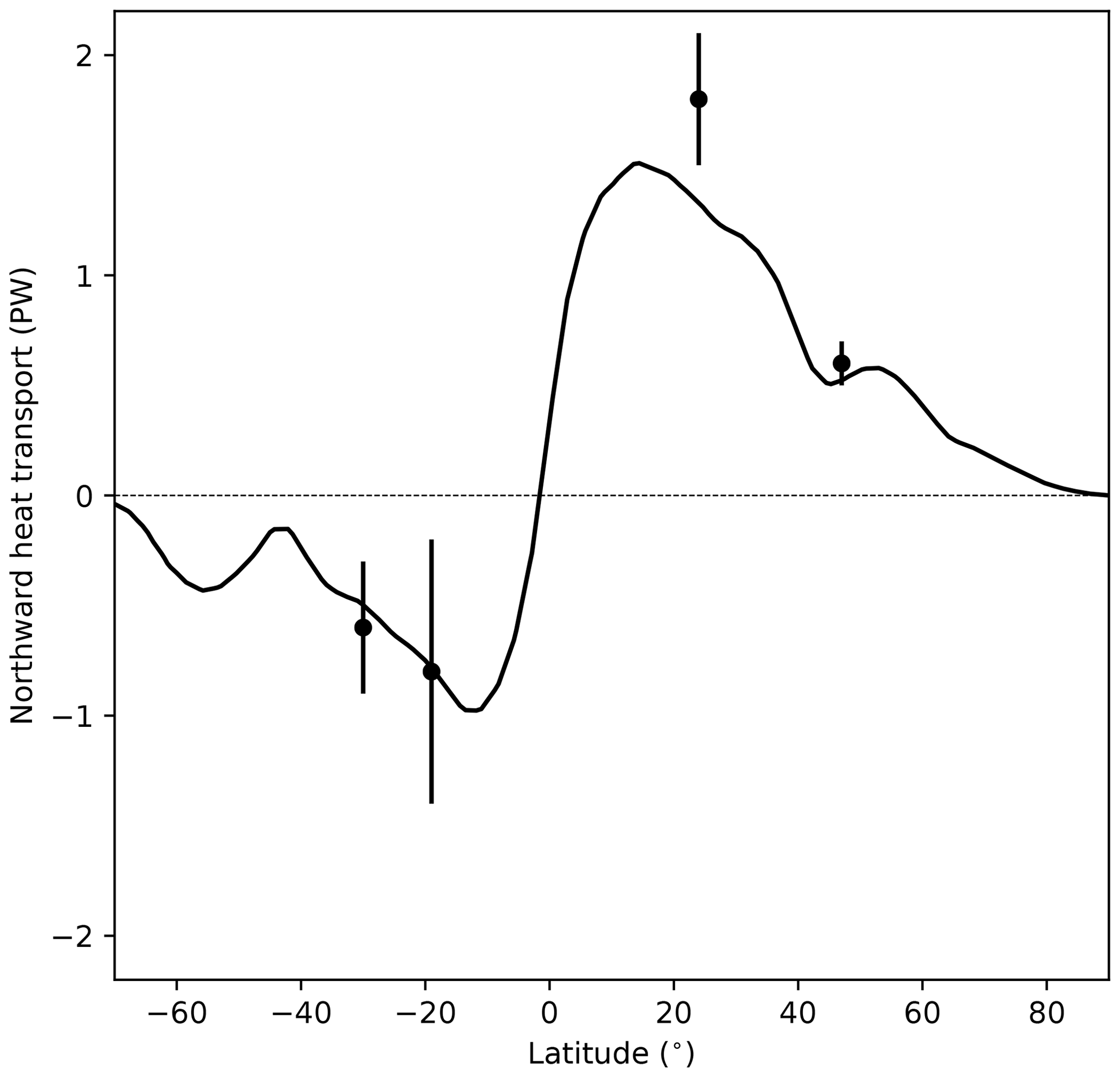
Figure 18 Northward heat transport in the global ocean in CanESM5 (in petawatts), with error bars showing the inverse estimate of Ganachaud and Wunsch (2003).

5.5 Sea ice

The seasonal cycles of sea-ice extent and volume are shown in Fig. 19. A major change from CanESM2 is seen in the sea-ice volume (Fig. 19b, d). CanESM2 simulated very thin ice and had about 40 % less Northern Hemisphere (NH) ice volume than in the Pan-Arctic Ice Ocean Modeling and Assimilation System (PIOMAS) reanalysis (Zhang and Rothrock, 2003; Schweiger et al., 2011). By contrast, CanESM5 has a larger NH ice volume than in CanESM2 (Fig. 19b). The amplitude and phase of the annual cycle in NH sea-ice volume in CanESM5 are similar to those in PIOMAS (Fig. 19b). In the Southern Hemisphere, CanESM5 also has a larger sea-ice volume and a seasonal cycle far more consistent with the global PIOMAS (GIOMAS) reanalysis product than CanESM2 (Fig. 19d).

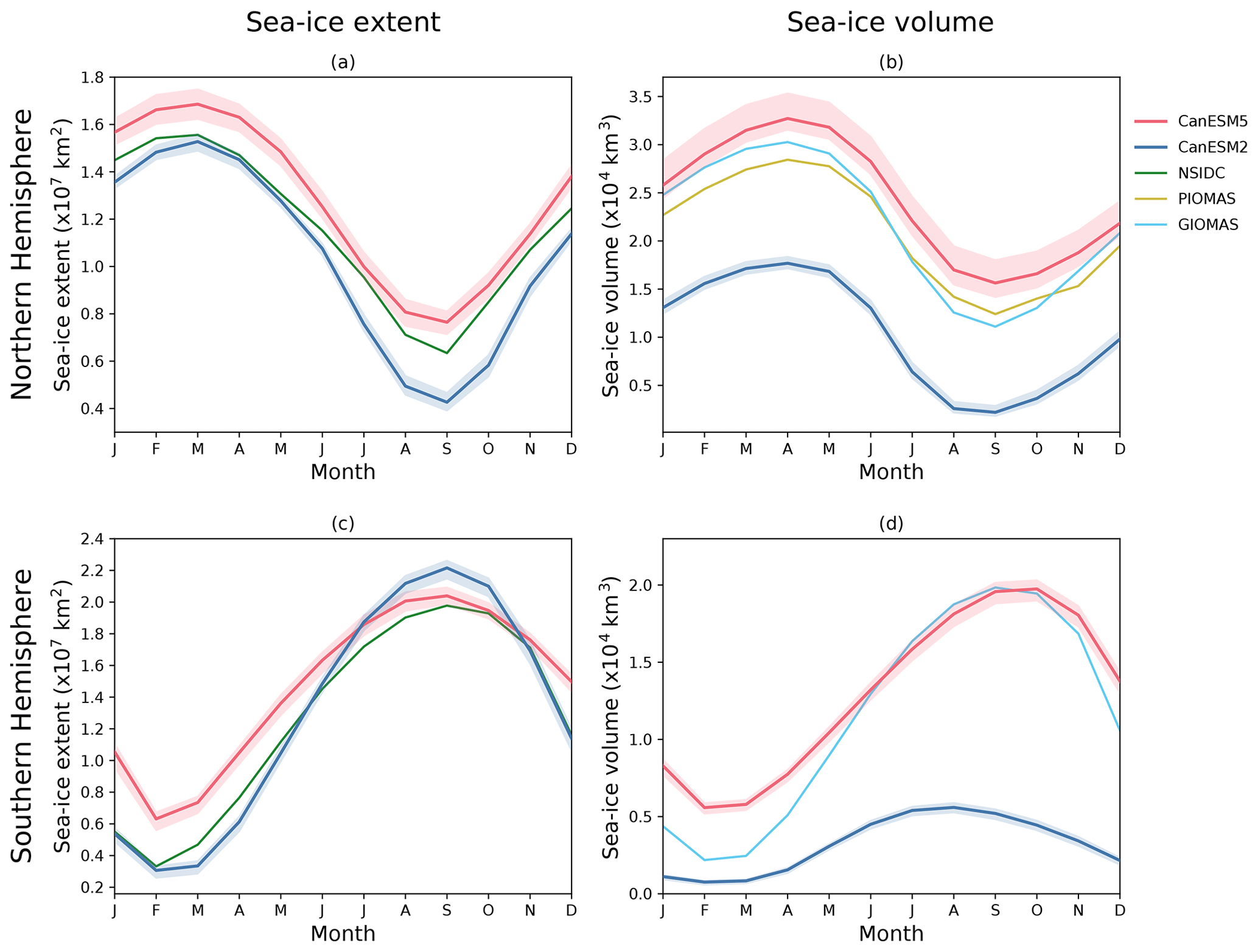
Figure 19 Seasonal cycles of sea-ice extent (a, c) and volume (b, d) in the Northern Hemisphere (a, b) and Southern Hemisphere (c, d) averaged over 1981 to 2010. Results are shown for CanESM2, CanESM5, the National Snow and Ice Data Center (NSIDC) satellite-based observations, and the PIOMAS and GIOMAS reanalyses.

While CanESM2 significantly underestimated NH sea-ice extent relative to satellite-based observations, CanESM5 generally overestimates the extent (Fig. 19a). The NH sea-ice extent biases are largest in the winter and spring. During the March maximum, excessive sea ice is present in the Labrador Sea and east of Greenland (Fig. 20a). In the summer and fall, the net NH extent bias is far smaller (Fig. 20c) and results from a cancellation between lower-than-observed concentrations over the Arctic basin and larger-than-observed concentrations around northeastern Greenland. Southern Hemisphere sea-ice extent biases are largest during the early months of the year, and in March the positive concentration biases are focused in the northeastern Weddell and Ross seas (Fig. 20b). In September, SH concentration biases between CanESM5 and the satellite observations are focused around the northern ice edge and are of varying sign (Fig. 20d).

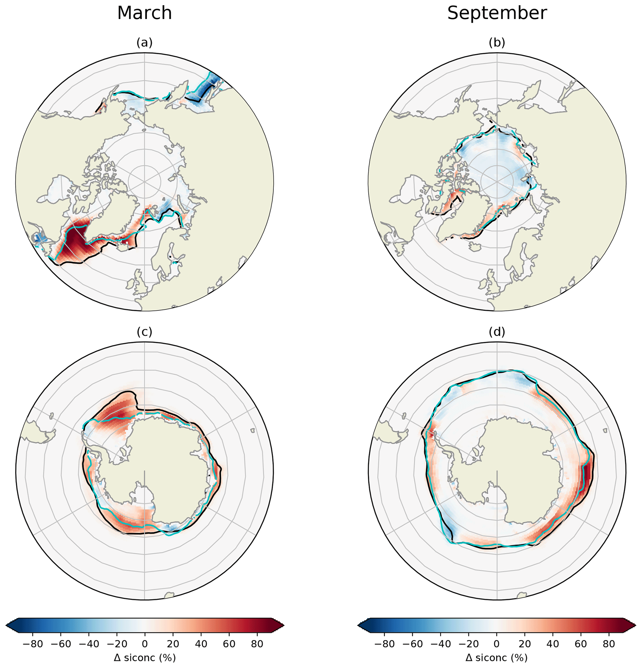
Figure 20 Sea-ice concentration biases between CanESM5 and NSIDC climatologies for the months of March (a, c) and September (b, d) in the Northern Hemisphere (a, b) and Southern Hemisphere (c, d). The solid black contour marks the ice edge (15 % threshold) in CanESM5, and the teal line marks the ice edge in the observations. Biases are based on the 1981 to 2010 climatology.

5.6 Ocean biogeochemistry

The standard configuration of CanESM5 has a significantly improved representation of the distribution of ocean biogeochemical tracers relative to CanESM2, despite using the same biogeochemical model (CMOC). For the three-dimensional distributions of DIC and NO₃, and the surface CO₂ flux, the RMSE, relative to observed distributions, was reduced by over a factor of 2 (Fig. 4). Ocean-only simulations, whereby NEMO was driven by CanESM2 surface forcing via bulk formulae, show similar skill to the CanESM5 coupled model. From this, we infer that changes in interior ocean circulation, rather than boundary forcing, are responsible for the improved representation of biogeochemical tracer distributions.

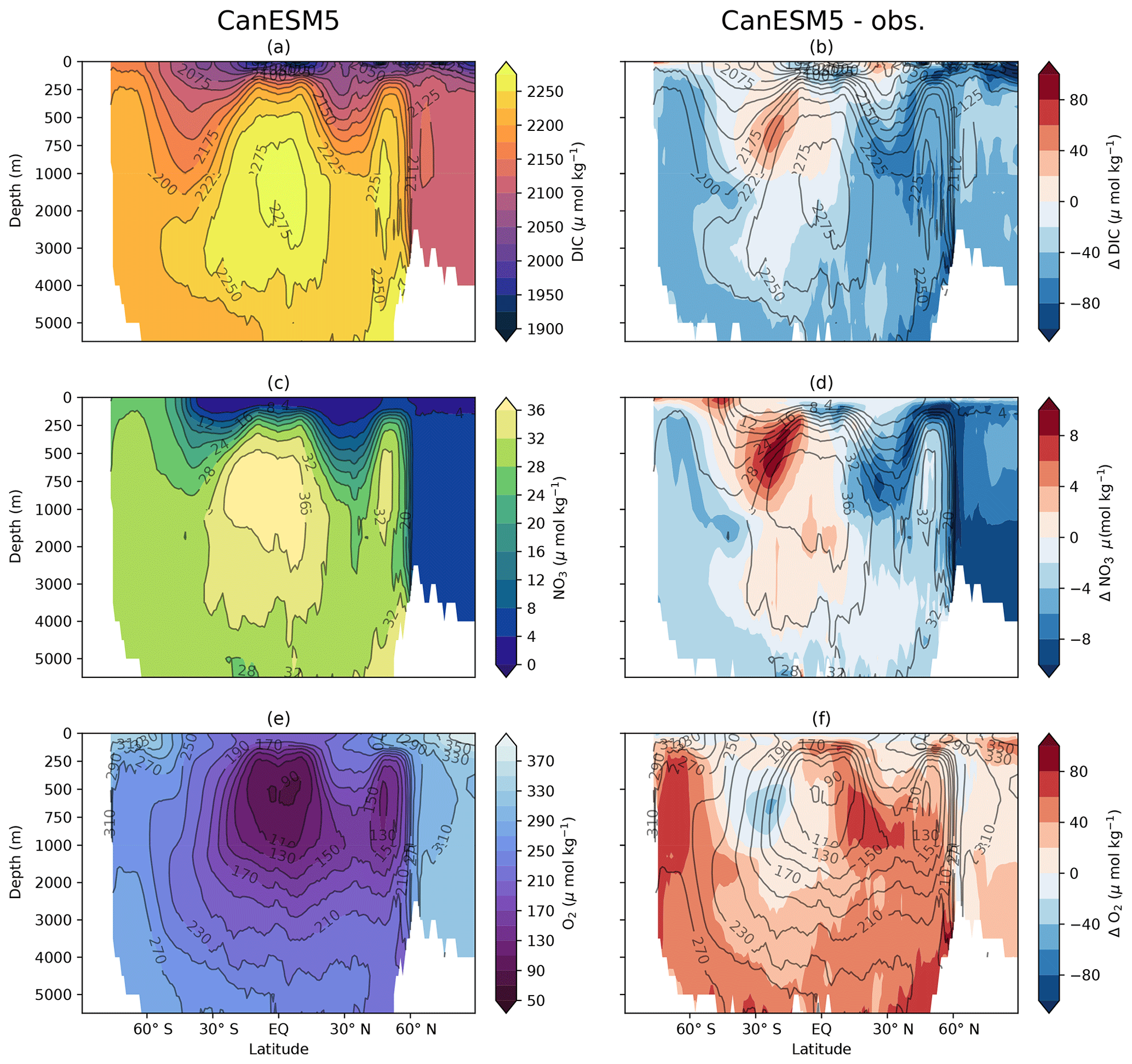
Figure 21 Zonal-mean sections of (a) dissolved inorganic carbon, (c) NO₃, and (e) O₂ in CanESM5, averaged over 1981 to 2010, and their biases relative to GLobal Ocean Data Analysis Project (GLODAP) v2 (b, d, f). Note that the depth scale on the y axis is non-uniform.

In CanESM5, the zonal-mean DIC concentration simulated by CMOC is generally lower than observed, by amounts reaching up to about 5 % (Fig. 21a, b). One exception to this is in the SH subtropical thermocline, on the northern flank of the Southern Ocean, which shows positive DIC biases between 250 and 1000 m. This area is also one of positive nitrate biases, whose magnitude is close to 30 % (Fig. 21d). Elsewhere, zonal-mean NO₃ concentrations are generally too low, particularly in the NH thermocline and the Arctic. CanESM5 has higher-than-observed concentrations of zonal-mean O₂ (Fig. 21f). As expected from saturation, biases are largest in the Southern Ocean and abyssal ocean, where CanESM5 is colder than observed. However, positive O₂ biases also occur at the base of the thermocline in the NH, where CanESM5 is too warm, suggestive of a biological origin.

The zonal-mean NO₃ biases identified at the thermocline level above are the result of partially cancelling biases between the Pacific and Atlantic basins (not shown). The Atlantic has negative NO₃ biases, largest near 1000 m. Meanwhile, there is an excessive accumulation of NO₃ centred at the base of the eastern Pacific thermocline. This buildup occurs due to the simplified parameterization of denitrification in CMOC. Within each vertical column, the amount of denitrification is set to balance the rate of nitrogen fixation and is distributed vertically proportional to the detrital remineralization rate. In reality, nitrogen fixation and denitrification are not constrained to balance within the water column at any one location, but rather denitrification proceeds within anoxic areas. A prognostic implementation of denitrification implemented into CanOE resolves this bias and will be discussed further in an upcoming article within this special issue.

Figure 22 (a) Ocean–atmosphere flux of CO₂ in CanESM5, averaged over 1981 to 2010, (b) the bias relative to Landschützer (2009), and (c) zonal-mean CO₂ flux in CanESM2, CanESM5, and Landschützer (2009) data. The flux is positive downward (into the ocean).

The atmosphere–ocean CO₂ flux pattern in CanESM5 correlates significantly better with estimates of the observed flux than that in CanESM2 (Fig. 4). The largest departures from the observations are positive biases in the southeastern Pacific, northwest Pacific, and northwest Atlantic (Fig. 22b). These are compensated by negative biases in the Southern Ocean and midlatitude northeast Pacific. In the zonal mean, CanESM2 had a large flux dipole in the Southern Ocean, which is significantly reduced in CanESM5, and attributable to improved circulation in the new NEMO ocean model and a reduction in Southern Ocean wind speed biases in CanAM5 (Fig. 22c).

5.7 Modes of climate variability

5.7.1 El Niño–Southern Oscillation

The El Niño–Southern Oscillation (ENSO) is a key component of climate variability on seasonal and interannual timescales. To evaluate CanESM5's representation of ENSO, the NINO3.4 index (average monthly SST anomaly in the region bounded by 5^∘ S, 5^∘ N, 170^∘ W, 120^∘ W) from the first 10 historical ensemble members is compared against the Hadley Centre Sea Ice and Sea Surface Temperature (HadISST) dataset. The skill of CanESM5 at representing the local and remote effects of ENSO is evaluated by correlating SST anomalies with the resulting NINO3.4 index (Fig. 23a, b). Within the equatorial Pacific, a positive ENSO event in CanESM5 leads to an increase in SSTs across the entire basin, whereas observations show negative SST anomalies in the western basin and positive anomalies in the central and eastern Pacific. ENSO in CanESM5 also has weaker teleconnections. The SSTs within the subtropical North and South Pacific gyres are more weakly anticorrelated to ENSO than observed. HadISST shows a negative North Atlantic Oscillation (NAO)-like pattern associated with ENSO, which is not present in CanESM5. The SST teleconnection in the tropical Indian and Atlantic oceans is well represented by the model.

The spectral peak in the historical ensemble members (Fig. 23c) occurs at around 3–5 years in general agreement with observations. Variability on decadal timescales has a large spread between ensemble members, likely due to differences in the strength of warming trends over the historical period. Higher-frequency variability at monthly to seasonal timescales is significantly lower than observed. The lower monthly variability can also be seen by examining month-by-month interannual variability of NINO3.4 (Fig. 23d). While January remains the month of peak variability, overall, the annual cycle of NINO3.4 variability is weaker in CanESM5. In observations, ENSO variability is at its minimum between April and June but in CanESM5 the minimum variability (depending on the ensemble member) tends to be between July and September.

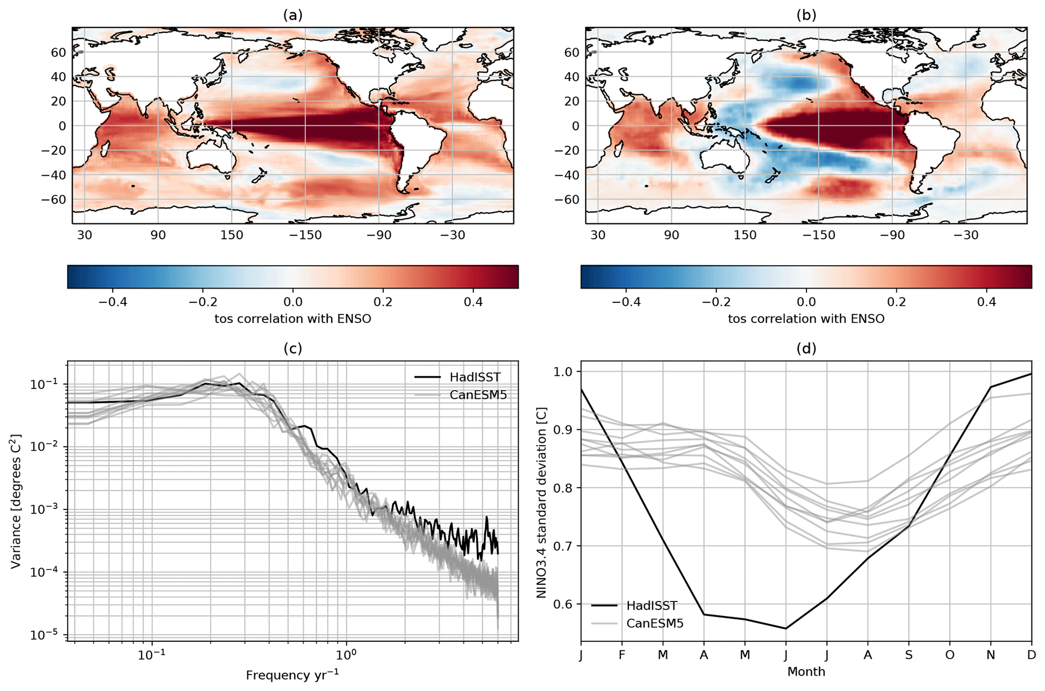
Figure 23 Characteristics of ENSO from and the HadISST observational product. Spatial maps in panels (a) and (b) are the regression of the SST monthly anomalies from 1850 to 2014 against the NINO3.4 index from (a) CanESM5 (historical ensemble member r1i1p1f1) and (b) HadISST. Temporal variability is summarized as power spectra (c) of the NINO3.4 index from HadISST and 10 historical ensemble members and the interannual variability of the NINO3.4 index by month (d) for CanESM5 and HadISST.

5.7.2 Annular modes

The Northern Annular Mode (NAM) is computed as the first EOF of extended winter (DJFM) sea-level pressure north of 20^∘ N for CanESM5 and ERA5 (Fig. 24a, b). The correlation between the CanESM5 and ERA5 patterns is 0.95. Despite the high degree of coherence, some differences between the model pattern and reanalysis are evident (Fig. 24). For example, CanESM5 has a positive centre in the north Pacific, not seen in ERA5, and the positive pattern across the North Atlantic is less continuous in CanESM5. This is a typical model bias (e.g. Bentsen et al., 2013). The first EOF in CanESM5 also explains about 8 % more variance than in the reanalysis.

Figure 24 First empirical orthogonal functions (EOFs) of sea-level pressure north of 20^∘ N (a, b) and south of 20^∘ S (c, d), representing the Northern Annual Mode (NAM) and Southern Annular Mode (SAM), respectively. The NAM is based on the extended winter DJFM season, and the SAM is based on monthly sea-level pressure. Results are shown for CanESM5 (a, c) and ERA5 (b, d), and the amount of variance explained by each EOF is given in brackets.

The Southern Annular Mode (SAM) is the dominant mode of climate variability in the Southern Hemisphere, with significant influences on atmospheric circulation, precipitation, and the Southern Ocean. We compute the SAM pattern as the first EOF of sea-level pressure south of 20^∘ S. The CanESM5 and ERA5 pattern correlation is 0.7. In CanESM5, the first EOF accounts for 13 % more variance than in the reanalysis. Despite such biases, these results confirm that CanESM5 captures the principal modes of tropical and midlatitude climate variability.

6 Climate response to forcing

6.1 Response to CO₂ forcing

The global-mean screen temperature change under the idealized CMIP6 DECK “abrupt-4xCO2” and “1pctCO2” experiments is shown in Fig. 2. From these simulations, three major benchmarks of the model's response to CO₂ forcing can be quantified (Table 3).

Table 3 Key sensitivity metrics: transient climate response (TCR), transient climate response to cumulative emissions (TCRE), and equilibrium climate sensitivity (ECS).

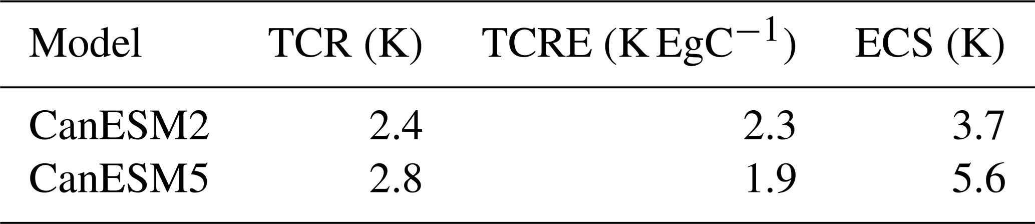
The transient climate response (TCR) of the model is given by the temperature change in the 1pctCO2 experiment, averaged over the 20 years centred on the year of CO₂ doubling (year 70), relative to piControl. For CanESM5, the TCR is 2.8 K, an increase of 0.4 K over that seen in CanESM2. The CanESM5 TCR is larger than that seen in any CMIP5 models and significantly higher than the CMIP5 mean value of 1.8 K (Flato et al., 2013). The likely range (ρ>0.66) of TCR was given by the IPCC AR5 as 1.0–2.5 K (Collins et al., 2013), while more recent observational based estimates quote a 90 % range of 1.2 to 2.4 K (Schurer et al., 2018), again subject to significant observational and methodological uncertainty.

The transient climate response to cumulative emissions (TCRE) incorporates the transient climate sensitivity together with the carbon sensitivity of the system (Matthews et al., 2009). It is defined as the ratio of global-mean surface warming to cumulative carbon emissions, over the 20 years centred on CO₂ doubling in the 1pctCO2 experiment, with units of K EgC⁻¹. The metric is of major policy relevance and is widely used to estimate the allowable emissions to reach given temperature targets. The TCRE of CanESM5 is 1.9 K EgC⁻¹, slightly lower than the CanESM2 value of 2.3 K EgC⁻¹. The reduction in TCRE occurs despite the fact that CanESM5 has a larger TCR than CanESM2 due to significantly larger uptake of CO₂ by the land biosphere in CanESM5 relative to CanESM2 in the 1pctCO2 experiment. As mentioned in Sect. 2.2, this is due to higher strength of the CO₂ fertilization effect in CanESM5 relative to CanESM2. As shown in Arora and Scinocca (2016), this leads to land carbon uptake in the 1pctCO2 simulation that is higher than in all CMIP5 models compared in Arora et al. (2013). Gillett et al. (2013) estimated the TCRE in 15 CMIP5 models to range from 0.8 to 2.4 K EgC⁻¹, and the IPCC AR5 likely range was assessed as 0.8 to 2.5 K EgC⁻¹.

The equilibrium climate sensitivity (ECS) is defined as the amount of global-mean surface warming resulting from a doubling of atmospheric CO₂, and a key measure of the sensitivity to external forcing. Given the long equilibration time of the climate system, it is common to estimate ECS from the relationship between surface temperature change and radiative forcing, over the course of the first 140 years of the abrupt-4xCO2 simulation (Gregory et al., 2004). Here, the ECS is calculated using the Gregory et al. (2004) regression method, after removing linear drift from the piControl following Forster et al. (2013). For CanESM5, the ECS is 5.6 K, a significant increase over the value of 3.7 K in CanESM2. Like TCR, the CanESM5 ECS value is larger than that seen in any CMIP5 models and significantly higher than the CMIP5 mean value of 3.2 K (Flato et al., 2013). The likely range for ECS was given by the IPCC AR5 as 1.5 to 4.5 K (Collins et al., 2013). CanESM5 falls outside this range, although it is worth noting that there are significant uncertainties in observational constraints of ECS. We also note, as above, that ECS is an emergent property in CanESM5 – no model tuning was done on the response to forcing.

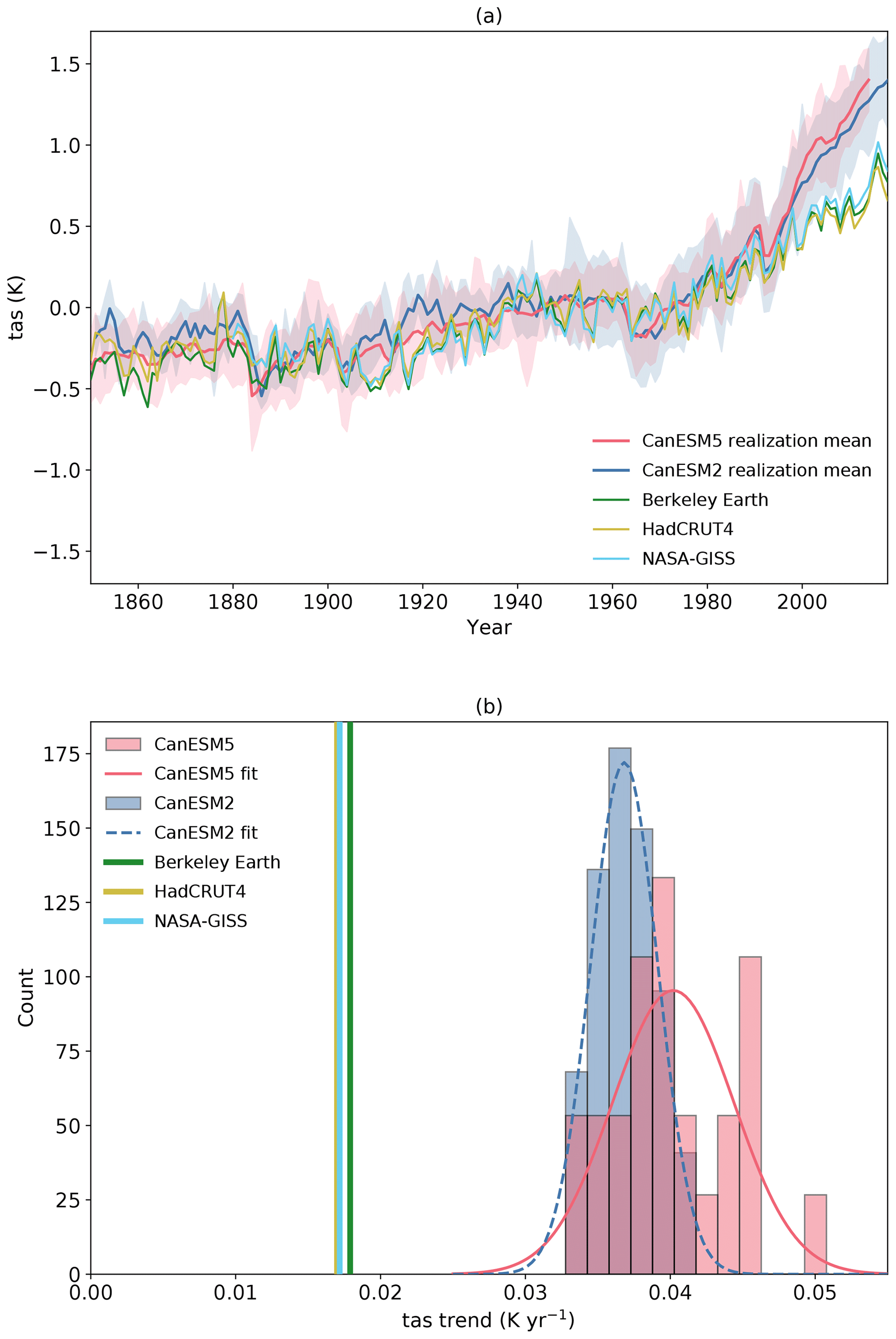
Figure 25 (a) Global-mean screen temperature in CanESM5, CanESM2, and various observational products and (b) histogram of historical trends over 1981 to 2014. In panel (a), the shaded envelopes represent the range over the CanESM2 50-member large ensemble and the CanESM5 25-member “p1” ensemble. In panel (b), fits of the normal distribution to the CanESM2 and CanESM5 distributions are also shown.

A detailed explanation of the reasons behind the increased ECS in CanESM2 over CanESM5 is beyond the scope of this paper. However, the effective radiative forcing (Forster et al., 2016) in CanESM5 due to abrupt quadrupling of CO₂ is very similar to that in CanESM2, suggesting that changes in feedbacks rather than forcings are the source of the higher ECS. Indications are that the increase in ECS is associated with cloud and surface albedo feedbacks, with sea ice likely playing an important role in the latter effect. The cloud albedo feedback is found to be sensitive to parameter settings in the cloud microphysics scheme. A more detailed examination of the changes in ECS due to cloud microphysics will be provided in a companion paper in this special issue (Cole et al., 2019). The examination of climate change over the historical period in the following section also reveals some further insights.

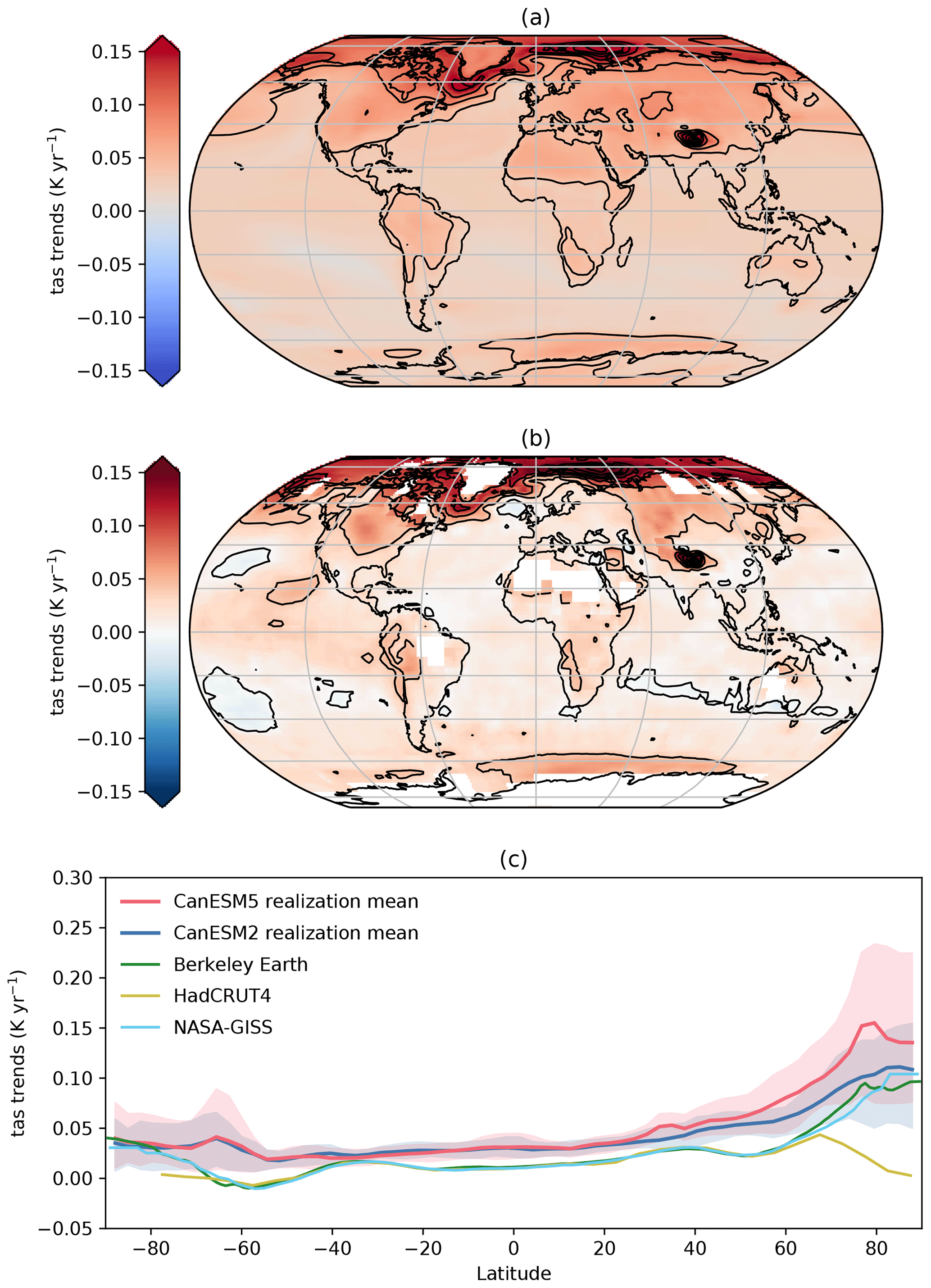
Figure 26 Surface temperature trends in CanESM5 (a), the difference in trend between CanESM5 and HadCRUT4 (b), and zonal mean of trends in CanESM2, CanESM5, and HADCRUT4 over 1981 to 2014 (c). The shaded envelopes in panel (c) represent the range over the CanESM2 50-member large ensemble and the CanESM5 25-member “p1” ensembles.

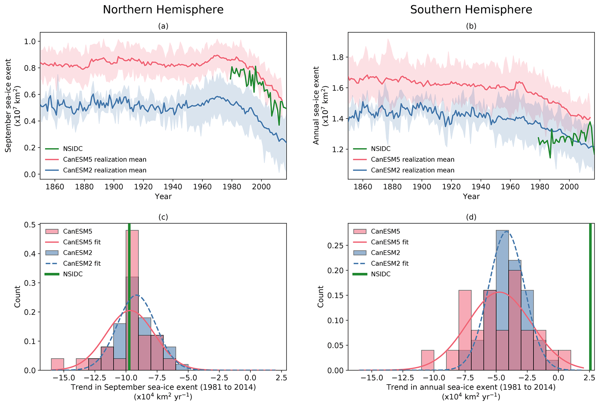
Figure 27 Time series of (a) sea-ice extent during September in the Northern Hemisphere and (b) the annual mean in the Southern Hemisphere in CanESM5, CanESM2, and NSIDC satellite-based observations. The histogram of trends over 1981 to 2014 is shown in the lower panels. The shaded envelopes represent the range over the CanESM2 50-member large ensemble and the CanESM5 25-member “p1” ensemble. Fits of the normal distribution to the CanESM2 and CanESM5 histograms are also shown.

6.2 Climate change over the historical period

In this section, we briefly discuss CanESM5-simulated changes in surface air temperature, sea ice, and carbon cycle fluxes over the historical period. We choose these as major emblematic variables of climate change. Here, we make use of the CanESM2 50-member large initial condition ensemble (Kirchmeier-Young et al., 2017; Swart et al., 2018). The 50 realizations in this ensemble were branched in the year 1950 from the five CanESM2 realizations submitted to CMIP5 and were forced by CMIP5 historical (1950 to 2005) and Representative Concentration Pathway (RCP) 8.5 (2006 to 2100) forcing.

6.2.1 Surface temperature changes

Global-mean surface temperature (GMST) changes in CanESM2 and CanESM5 are generally consistent with the observations over the period from 1850 to around the end of the 20th century (Fig. 25a). However, from 2000 to 2014, the increase in GMST is larger in the models than observed. Possible reasons for the divergence are (i) forcing errors in the CMIP5 and/or CMIP6 forcing datasets, (ii) natural internal variability, (iii) incorrect partitioning of heat across components of the climate system, or (iv) a higher climate sensitivity in the model than in the real world. The 25 realizations of CanESM5 (and 50 realization of CanESM2) provide a good estimate of the contribution of internal variability in the model. The observations fall outside the range of this variability, and hence this cannot account entirely for the divergence between the model and observations (assuming the model correctly captures the scale of internal variability). Trends computed from 1981 to 2014 show that the models are warming at roughly twice the observed rate over this period (Fig. 25b). The spread across the 25 realizations from CanESM5 and 50 realizations from CanESM2 does not encompass the observations, reinforcing the point above. CanESM5 warms more rapidly than CanESM2, on average, as would be expected from its higher ECS and TCR. There is, however, significant overlap across the distribution of warming rates across the CanESM5 and CanESM2 ensembles. Interestingly, the lower tail of the trend probability distribution functions aligns for the two models, but CanESM5 has a broader distribution and a larger tail of high warming realizations.

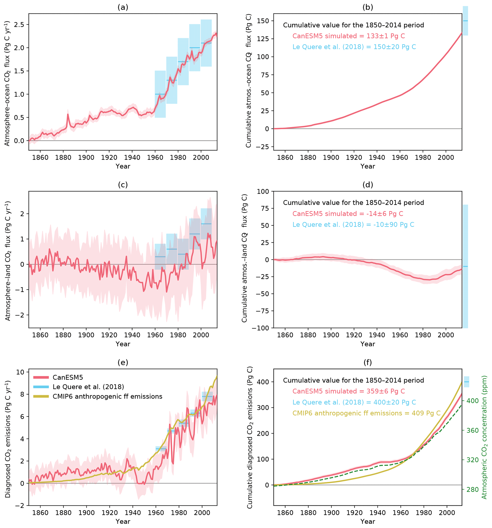
Figure 28 Annual (a, c, e) and cumulative (b, d, f) global values of simulated atmosphere–ocean and atmosphere–land CO₂ fluxes, and diagnosed anthropogenic fossil fuel emissions, shown in blue colour. The model values are shown as mean ±1 standard deviation range and calculated based on the 25 ensemble members of the historical simulation. Model values are compared against estimates from Le Quéré et al. (2018).

The pattern of surface warming in CanESM5 over the historical period is shown in Fig. 26a. The canonical features of global warming are consistent between the model and observations: greater warming over land than ocean and Arctic amplified warming. The zonal-mean warming trends (Fig. 26c) show that both CanESM2 and CanESM5 warmed more than the observations over most latitudes. Divergence between simulated and observed warming rates is largest in the high latitudes, notably over the Southern Ocean and north of 40^∘ N. The larger warming in the CanESM5 ensemble mean, relative to the CanESM2 ensemble mean, largely occurs over the Arctic. However, there is a very large variability in Arctic warming trends in CanESM5, which most likely are responsible for the spread in GMST trends noted above. Some realizations have lower trends, which overlap with observed warming, while others exhibit considerably higher rates of Arctic warming. Observed warming rates over the Arctic are also some of the most uncertain due to data sparsity (HadCRUT is masked where observations are not available).

6.2.2 Sea-ice changes

CanESM5 closely reproduces the observed reduction in Arctic September sea-ice extent (Fig. 27a). The trends from both the 50 CanESM2 ensemble members and the 25 CanESM5 ensemble members show a broad spread due to internal variability (Fig. 27c). The observed trends lie close to the centre of the model distribution of trends. Given that CanESM5 warms more rapidly than observed, the sea-ice sensitivity (rate of sea-ice decline normalized by the rate of warming) is likely too low (Rosenblum and Eisenman, 2017; Winton, 2011).

In the Southern Hemisphere, observed annual-mean Antarctic sea-ice extent showed a tendency to increase before dramatic declines in the past few years (Fig. 27b). Both CanESM5 and CanESM2 show consistent declines over the historical period, with CanESM2 matching the climatological extent more closely.

6.2.3 Historical carbon cycle changes

The simulated global atmosphere–ocean (F_O) and atmosphere–land (F_L) CO₂ fluxes are shown in Fig. 28 for the historical period, along with their cumulative values over time. Also shown are the diagnosed anthropogenic fossil fuel emissions (E) that are consistent with the specified CO₂ pathway over the historical period, corrected for any drift in the model's pre-industrial control simulation (see Appendix F). The simulated values of F_L, F_O, and E are compared against estimates from the Global Carbon Project (Le Quéré et al., 2018).

In Fig. 28a, the simulated global atmosphere–ocean CO₂ fluxes compare reasonably well with observation-based estimates from Le Quéré et al. (2018) for the decades of the 1960s through the 2000s, although the simulated cumulative value of 133±1 Pg C for the 1850–2014 period is on the lower end of the observation-based estimate of 150±20 Pg C (Fig. 28b). In contrast, the simulated mean atmosphere–land CO₂ fluxes (Fig. 28c) for the decades of the 1960s to the 2000s are lower than their observation-based estimates from Le Quéré et al. (2018). This is despite the fact that the land carbon uptake in the 1pctCO2 simulation for CanESM5 is highest amongst all CMIP5 models reported in Arora et al. (2013). The reason for this conundrum is a topic for future investigation but might relate to differences in forcing (aerosols) in the historical and 1pctCO2 experiments. The cumulative atmosphere–land CO₂ flux of $-\mathrm{14}\pm \mathrm{6}$ Pg C over the 1850–2014 period, however, compares well with the observation-based estimate of $-\mathrm{10}\pm \mathrm{90}$ Pg C (Fig. 28d). The caveat here, of course, is the large uncertainty range in the observation-based estimate of net cumulative atmosphere–land CO₂ flux (Appendix F). The reason the model's simulated cumulative uptake of $-\mathrm{14}\pm \mathrm{6}$ Pg C over the 1850–2014 period compares well with the observation-based estimate of $-\mathrm{10}\pm \mathrm{90}$ Pg C, despite its weaker carbon sink since the 1960s (Fig. 28c), is likely because the carbon source from land use change emissions is also lower.

Figure 28e–f show the allowable diagnosed fossil fuel emissions and their cumulative values for the 1850–2014 period. The cumulative diagnosed fossil fuel emissions of 359±6 Pg C from the model for the period of 1850–2014 are somewhat lower than the CMIP6 and Le Quéré et al. (2018) estimates of 409 and 400±20 Pg C, respectively.

7 Conclusions

CanESM5 is the latest coupled model from the Canadian Centre for Climate Modelling and Analysis. Relative to its predecessor, CanESM2, the model has new ocean, sea-ice, and coupling components, and includes updates to the atmospheric and land surface. The model produces a stable pre-industrial control climate, and notwithstanding some significant biases, CanESM5 is able to reproduce many features of the historical climate. Objective global skill metrics show that CanESM5 improves the simulation of observed large-scale climate patterns, relative to CanESM2, for most variables surveyed. A notable feature of CanESM5 is its high equilibrium climate sensitivity of 5.6 K, an emergent property of the updated physics described above. This higher climate sensitivity appears to be driven by increased cloud and sea-ice albedo feedbacks in CanESM5. The first major science application of CanESM5 is for CMIP6, with over 50 000 years of CanESM5 simulation and more than 100 PB of data submitted to the publicly available CMIP6 archive. The model source code is also openly published for the first time. Going forward, CanESM5 will continue to be used for climate science applications in Canada.

Appendix A: Exchanges through the coupler

Figure A1 Schematic showing the ordering of exchanges between CanCPL and CanAM and CanNEMO. Prognostic fields (P_O) are passed from NEMO to the coupler, remapped, and passed to CanAM. Fluxes (F_A) are passed from CanAM, remapped in CanCPL, and passed NEMO to complete the next coupling cycle. Superscripts denote the coupling cycle; e.g. prognostic fields from NEMO are passed to CanCPL at the end of cycle “n”, remapped, and used in CanAM during cycle “n+1”.

Table A1 Fields received by CanAM from CanCPL. The representative area may be the full AGCM grid cell (land, ocean, and ice), “C”; open ocean, “O”, sea ice, “I”; or the combination. Fields may be instantaneous, “inst”, or averaged over the coupling cycle, “avg”.

Table A2 Fields sent from CanNEMO to CanCPL. Descriptions are as in Table A1.

Table A3 Fields received by CanNEMO from CanCPL. Descriptions are as in Table 1.

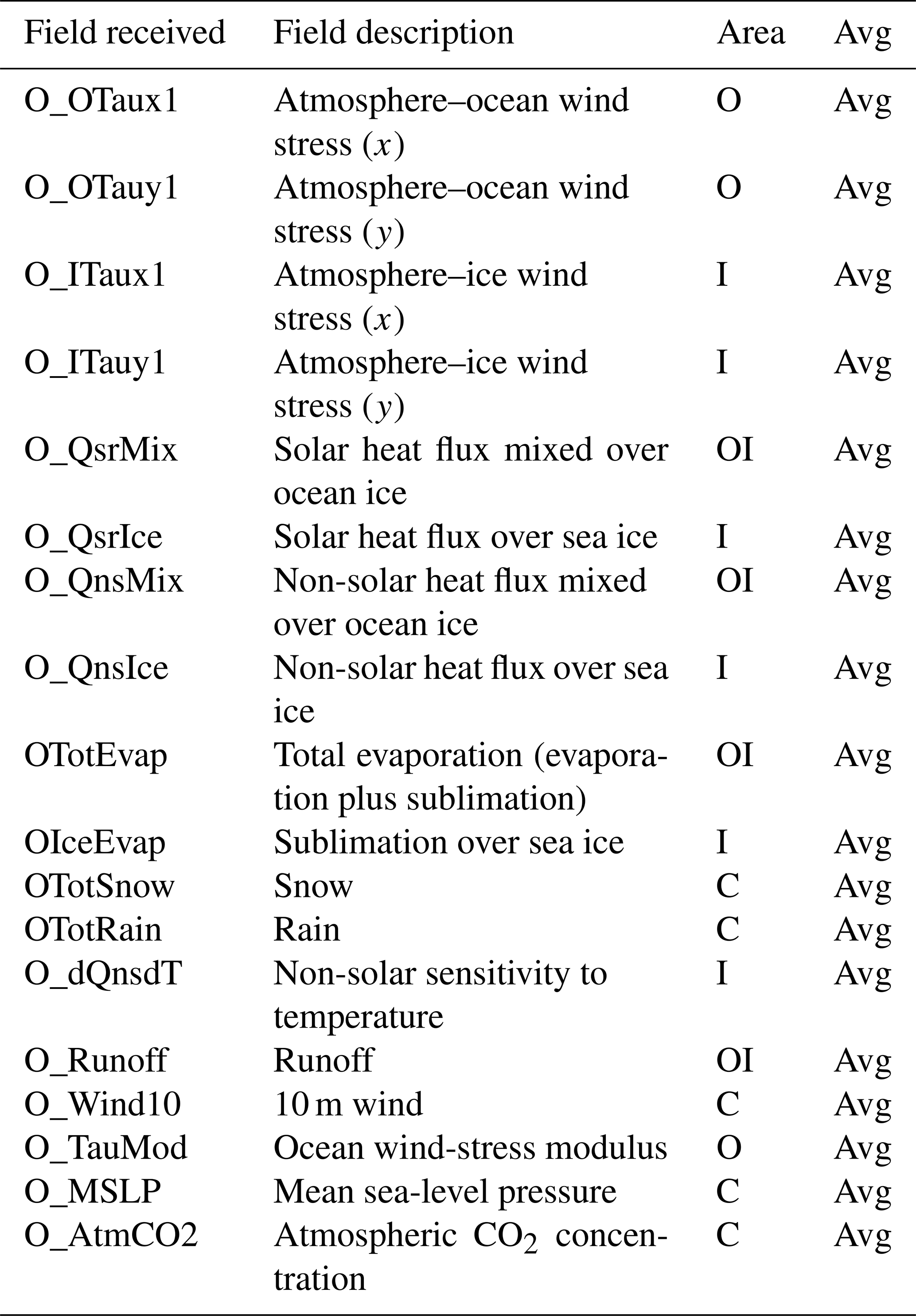
Table A4 Fields sent from CanAM to CanCPL. Descriptions are as in Table 1.

Appendix B: Code management and model infrastructure

Table B1 Code management.

Table B2 Process for running CanESM.

Appendix C: Code optimization

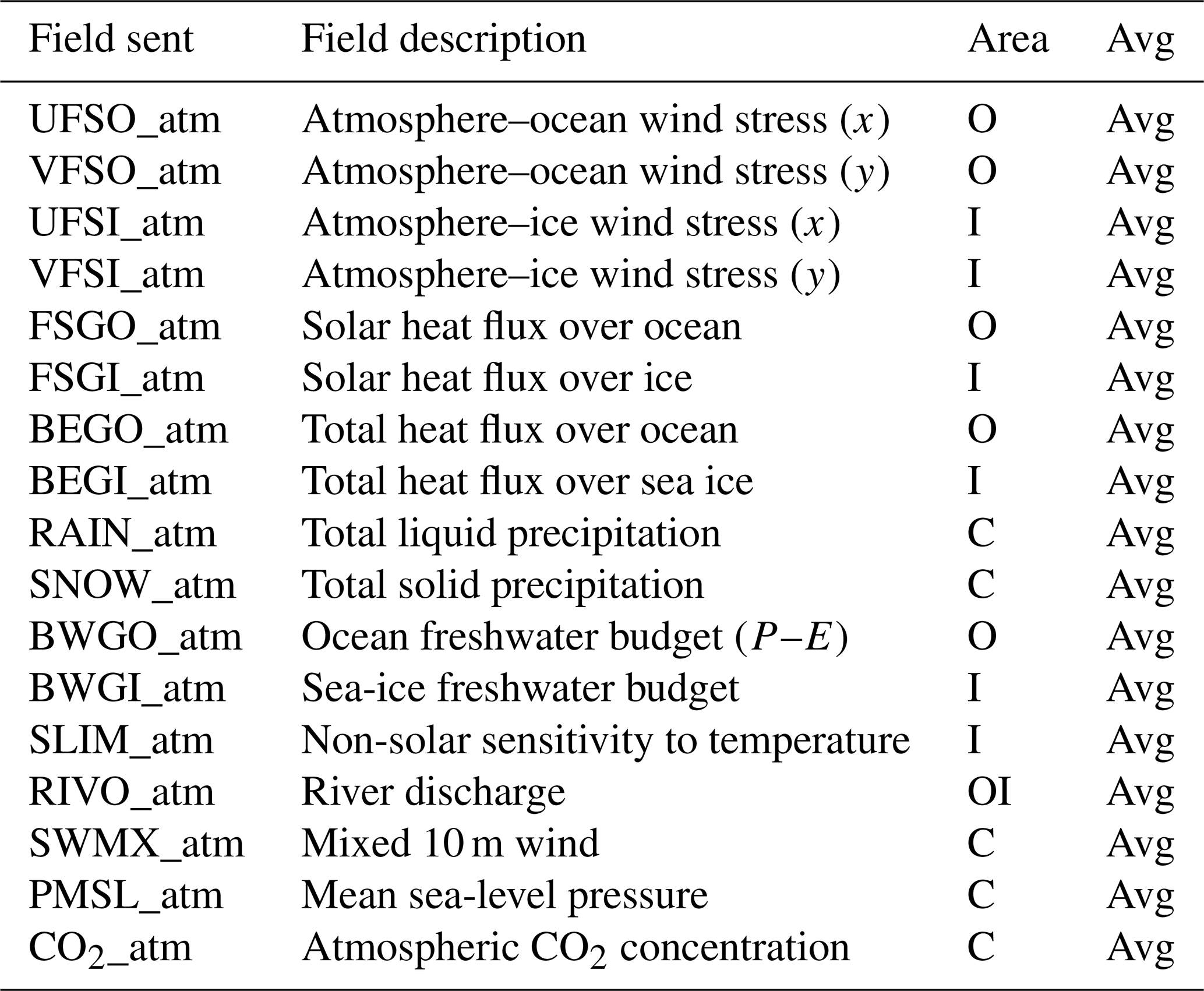
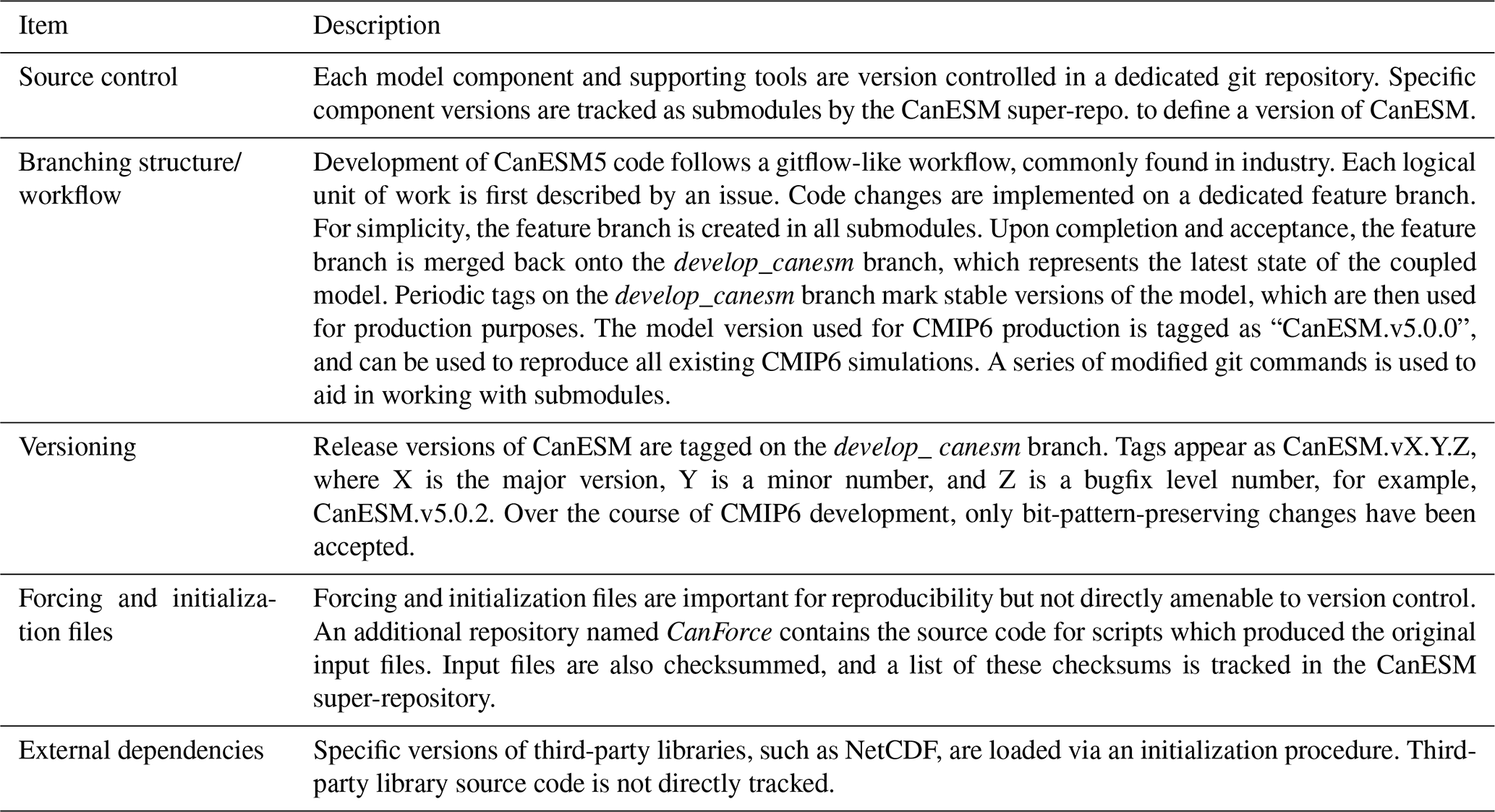
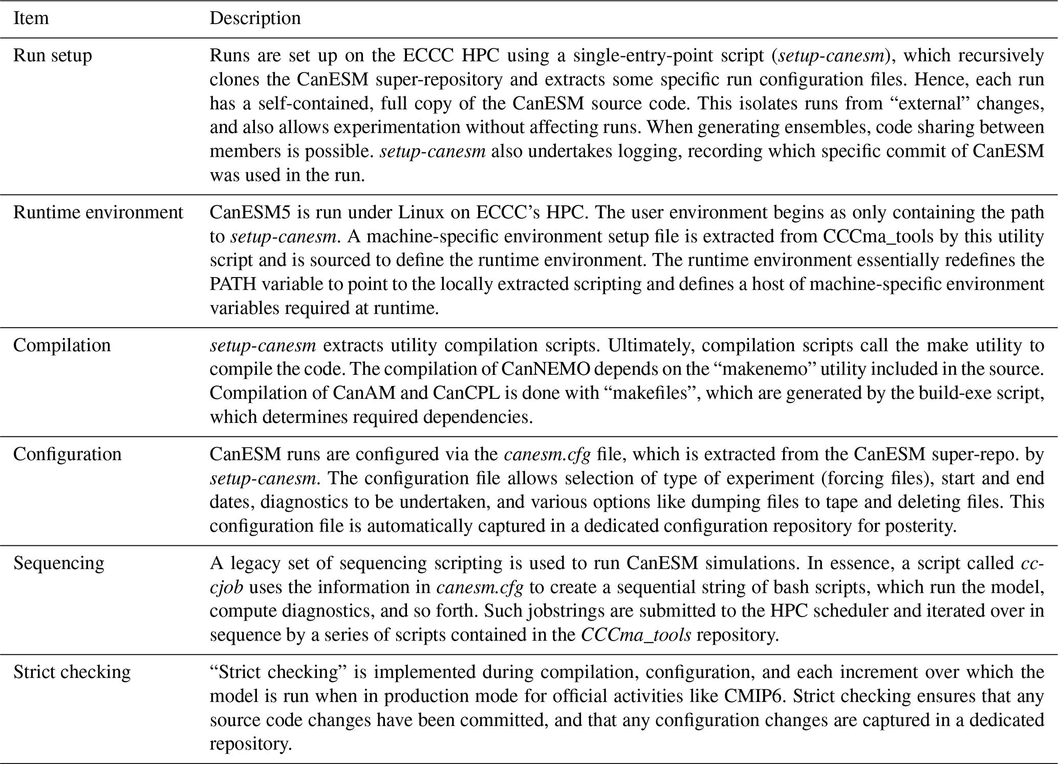
Table C1 Description of optimization improvements to CanESM5. See Fig. 1 for a graphical representation.

Appendix D: CMIP6 MIP participation and model variants

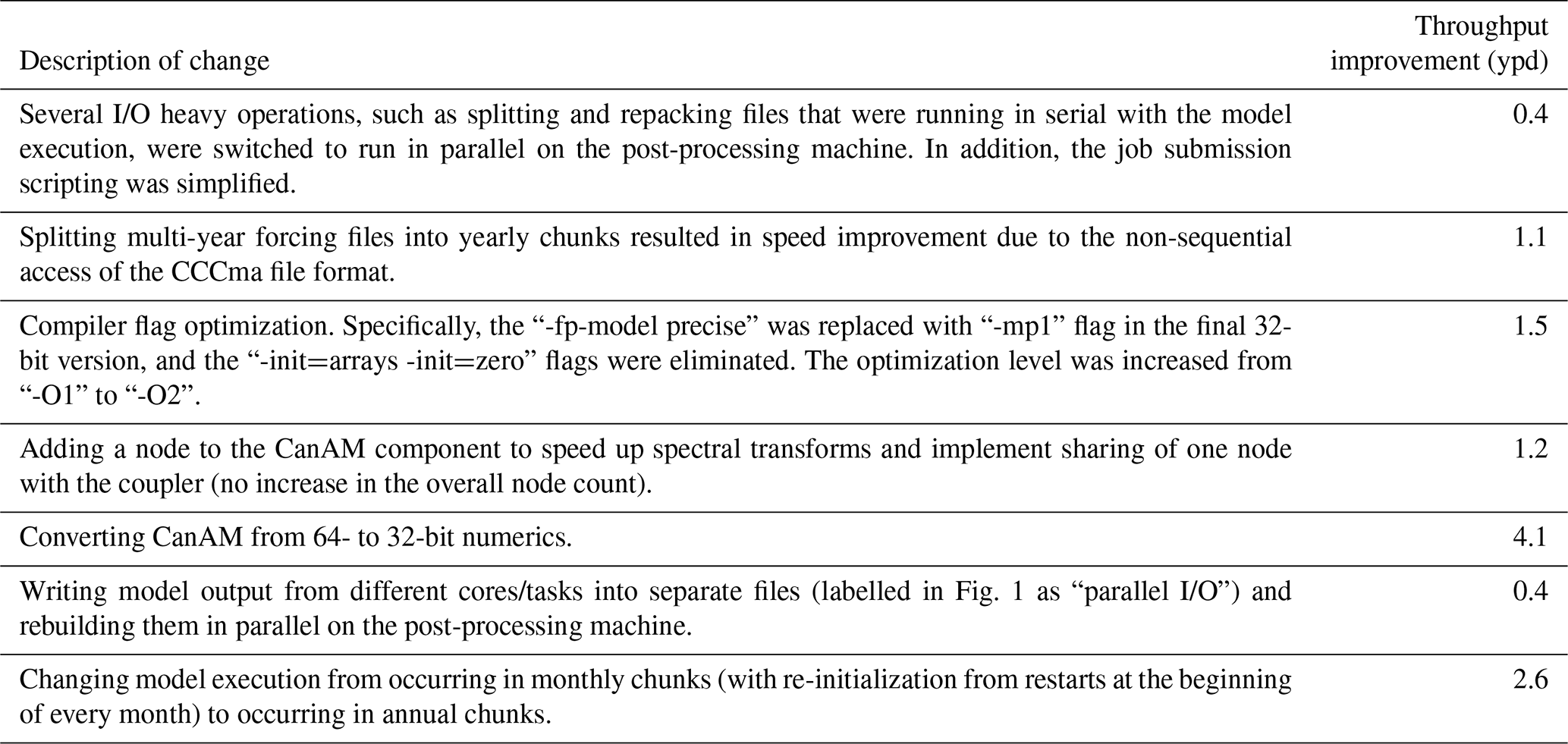
Table D1 List of MIPs and model variants of CanESM5 planned for submission to CMIP6.

Appendix E: Comparison between p1 and p2

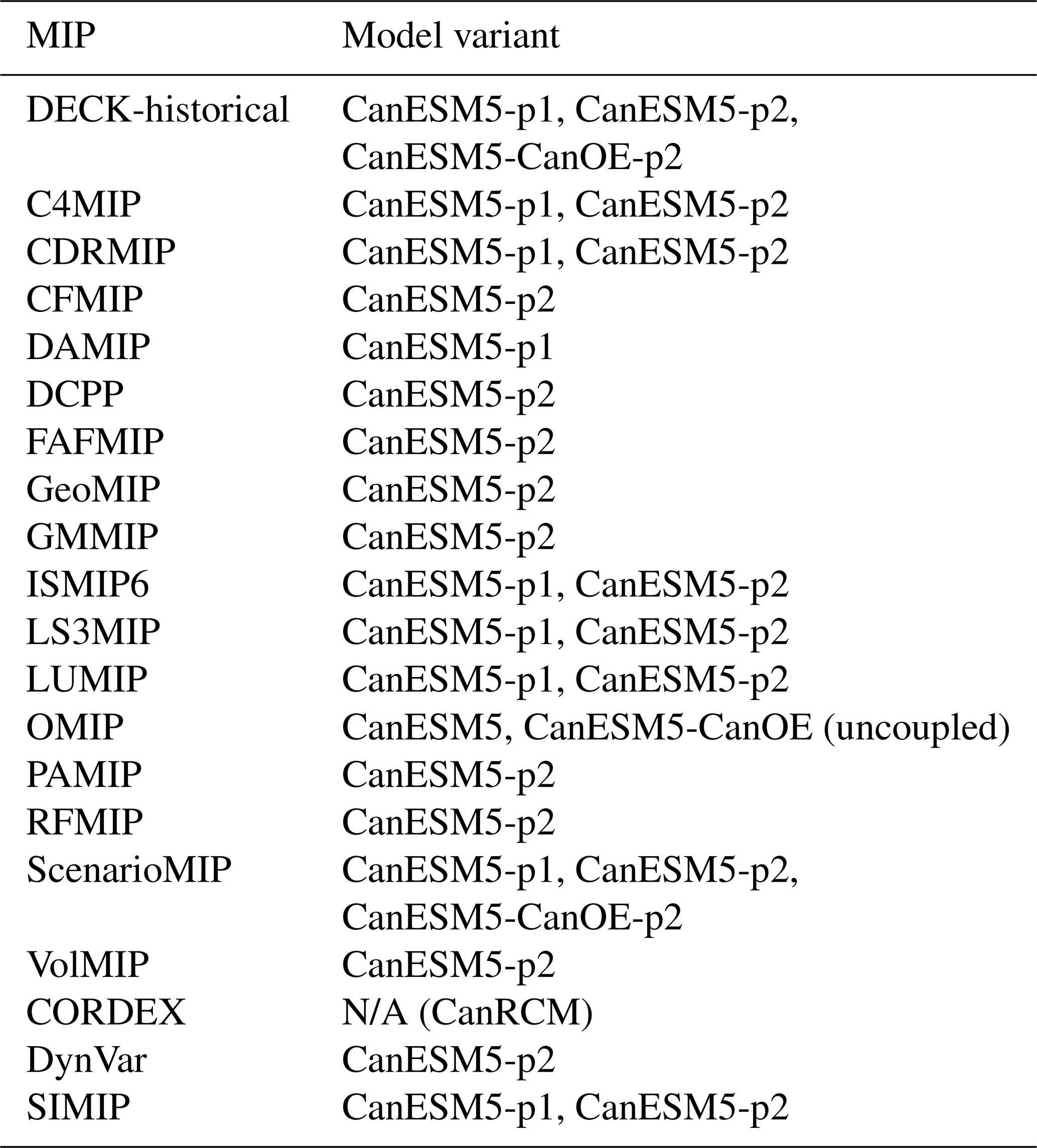
Sections 2.5 and 3.4 described the technical differences between perturbed physics members p1 and p2, submitted to the CMIP6 archive. Here, we provide a preliminary analysis of the differences between the two model variants.

Figure E1 shows surface air temperature and precipitation averaged over 200 years of the piControl experiment for p1, p2, and the difference between them. Notable in the differences are the “cold” spots in Antarctica, which arise from a misspecified land fraction in p1 and were resolved in p2. Otherwise there are no significant differences.

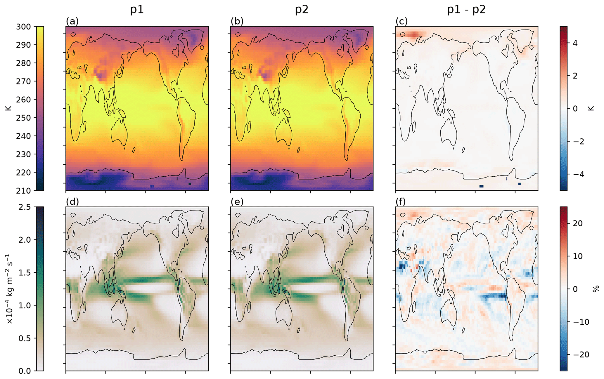
Figure E1 Climatologies of surface air temperature (a, b) and precipitation (d, e), computed over 200 years of the piControl simulation of the p1 (a, d) and p2 (b, e) model variants, and the differences between p1 and p2 (c, f).

Figure E2 shows the ocean surface wind stress. The blockiness of the field in p1 is evident as a result of conservative remapping from CanAM. In p2, bilinear remapping was used and the field is smooth on the NEMO grid. The non-smooth nature of wind stress in p1 resulted in, for example, banding in vertical ocean velocities at 100 m depth, as also shown in Fig. E2d. This does not occur in p2.

The response to CO₂ forcing in the 1pctCO2 experiments in p1 and p2 is shown in Fig. E3. The global-mean top-of-atmosphere radiation (Fig. E3a) and surface air temperature (Fig. E3b) responses are indistinguishable, and hence the TCR of these model variants is the same. The ocean is cooler, on average, in p2, but the perturbative responses in p1 and p2 are similar (Fig. E3c). Ocean surface CO₂ flux is also statistically indistinguishable between the variants (Fig. E3d).

Figure E2 Climatologies of surface ocean zonal wind stress (a, b) and vertical velocity near 100 m depth (d, e) computed over 200 years of the piControl simulation of the p1 (a, d) and p2 (b, e) model variants, and the differences between p1 and p2 (c, f). Results are shown on the native NEMO grid. The insets show an enlargement of the Southern Ocean south of Australia.

Maps of the perturbative response, computed as the mean over the 20 years centred on CO₂ doubling in the 1pctCO2 experiments, minus the piControl experiment, are shown in Figs. E4 and E5. There are no fundamental differences in the surface climate response between the two model variants.

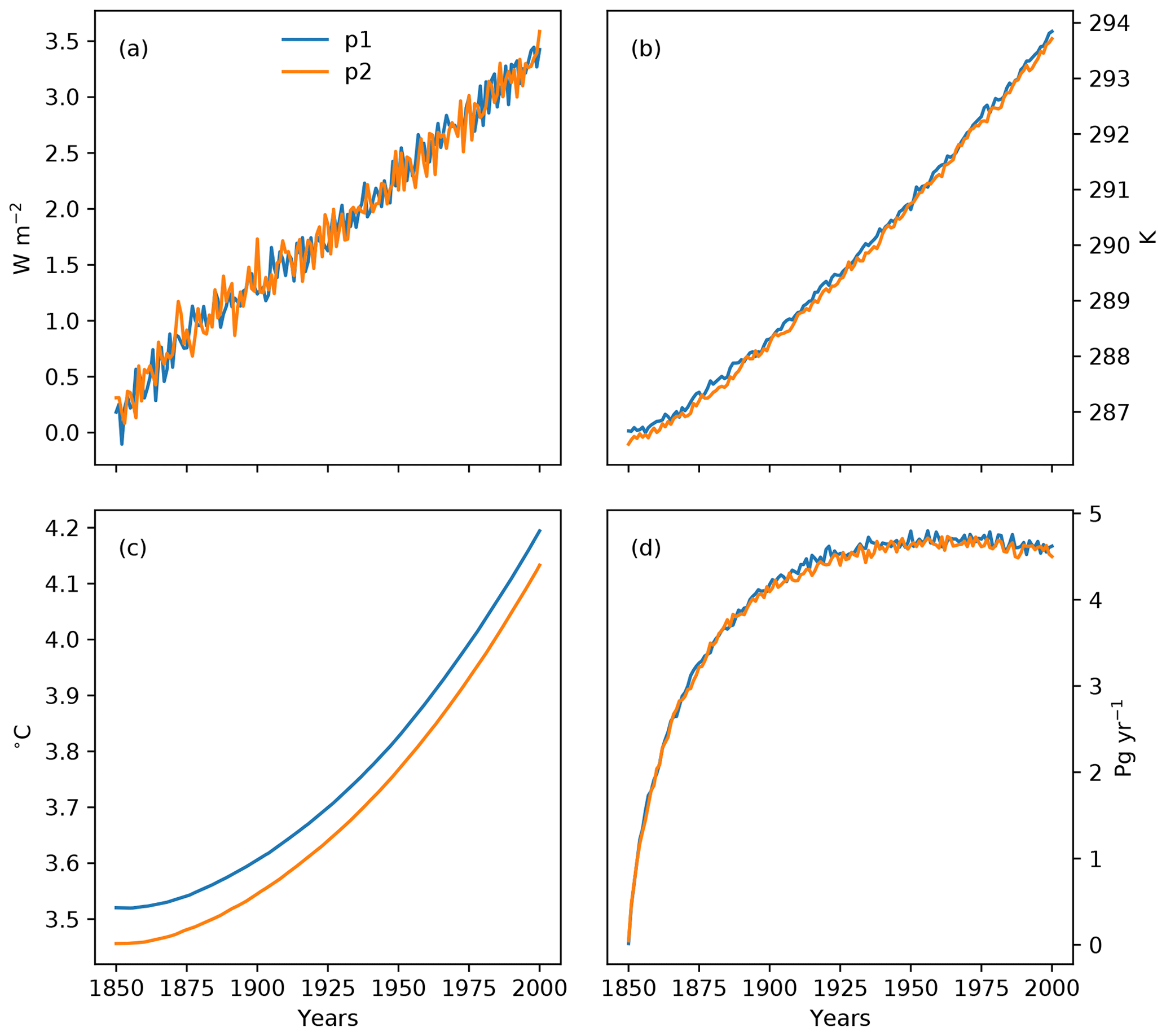
Figure E3 Global averages of (a) top-of-atmosphere net radiative flux, (b) surface air temperature, (c) volume-averaged ocean temperature, and (d) surface ocean CO₂ flux in the 1pctCO2 simulations from the p1 and p2 model variants.

Figure E4 Perturbation of surface air temperature (a, b) and precipitation (d, e) computed as the mean over the 20 years centred on CO₂ doubling in the 1pctCO2 experiment, minus the mean from 200 years of the piControl simulation of the p1 (a, d) and p2 (b, e) model variants, and the differences between p1 and p2 (c, f).

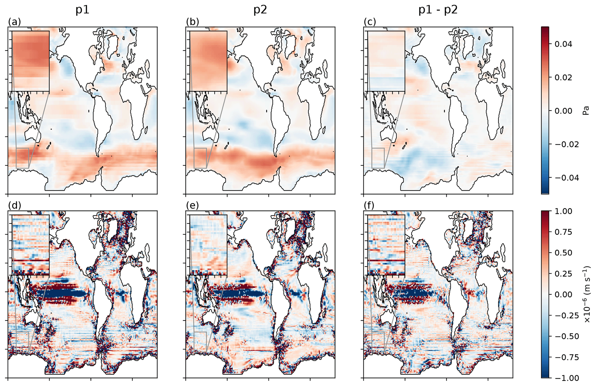
Figure E5 Perturbations of surface ocean zonal wind stress (a, b) and vertical velocity near 100 m depth (d, e) computed as the mean over the 20 years centred on CO₂ doubling in the 1pctCO2 experiment, minus the mean over 200 years of the piControl simulation of the p1 (a, d) and p2 (b, e) model variants, and the differences between p1 and p2 (c, f). Results are shown on the native NEMO grid. The insets show an enlargement of the Southern Ocean south of Australia.

Appendix F: Data sources, variables, and derived quantities

In Fig. 28, the diagnosed allowable anthropogenic fossil fuel emissions are calculated via Eq. (F1):

$$\begin{array}{}\text{(F1)}& {\displaystyle \frac{\text{d}\left[{\mathrm{CO}}_{\mathrm{2}}\right]}{\text{d}t}}=E-F_{\text{L}}-F_{\text{O}}=E-({F^{\prime }}_{\text{L}}-E_{\text{LUC}})-F_{\text{O}}.\end{array}$$

In these historical simulations, the concentration of atmospheric CO₂ is specified (that is, the term d[CO₂]∕dt is known) and the model's land and ocean carbon cycle components simulate atmosphere–land (F_L) and atmosphere–ocean (F_O) CO₂ fluxes, respectively. The $F_{\text{L}}=F_{\text{L}}-E_{\text{LUC}}$ term includes natural atmosphere–land CO₂ flux (F_L) and the emissions associated with land use change (E_LUC) which are calculated interactively in the model in response to the historical increase in cropland area. As a result, the term E can be calculated and represents the allowable anthropogenic fossil fuel emissions. Le Quéré et al. (2018) do not provide a direct value of net cumulative atmosphere–land CO₂ flux (F_L). Instead, they separately provide estimates of cumulative values of F_L (185±50 Pg C) and E_LUC (195±75) in their Table 8. Here, we calculate observation-based value of $F_{\text{L}}=F_{\text{L}}-E_{\text{LUC}}=\mathrm{185}-\mathrm{195}=-\mathrm{10}$ Pg C and its uncertainty as 90 Pg C; the uncertainty is calculated as $\sqrt{({\mathrm{50}}^{\mathrm{2}}+{\mathrm{75}}^{\mathrm{2}})}=\mathrm{90.13}$ Pg C. The large uncertainty range for the observation-based estimate of cumulative F_L is therefore due to large uncertainties in both land use change emissions and the natural atmosphere–land CO₂ flux.

Table F1 List of figures, CanESM5 CMIP6 variables, and observations used, and the time periods of analysis in the main text. See Table F3 for a definition of variable names. “n/a” indicates “not applicable”.

Table F2 List of observational products used.

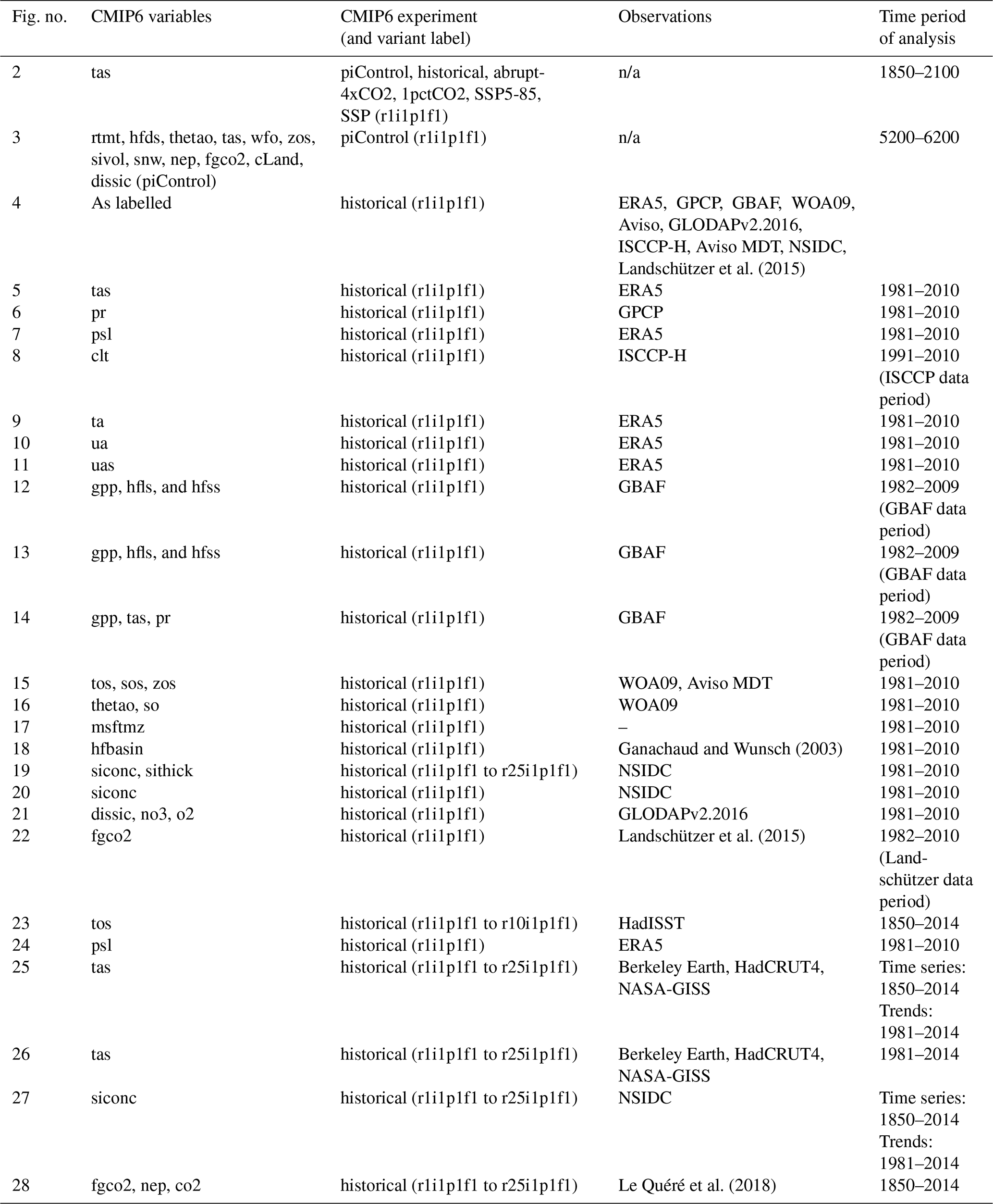
Table F3 List of CMIP6 variable names used and their long names.

Appendix G: Wetland extent and wetland methane emissions

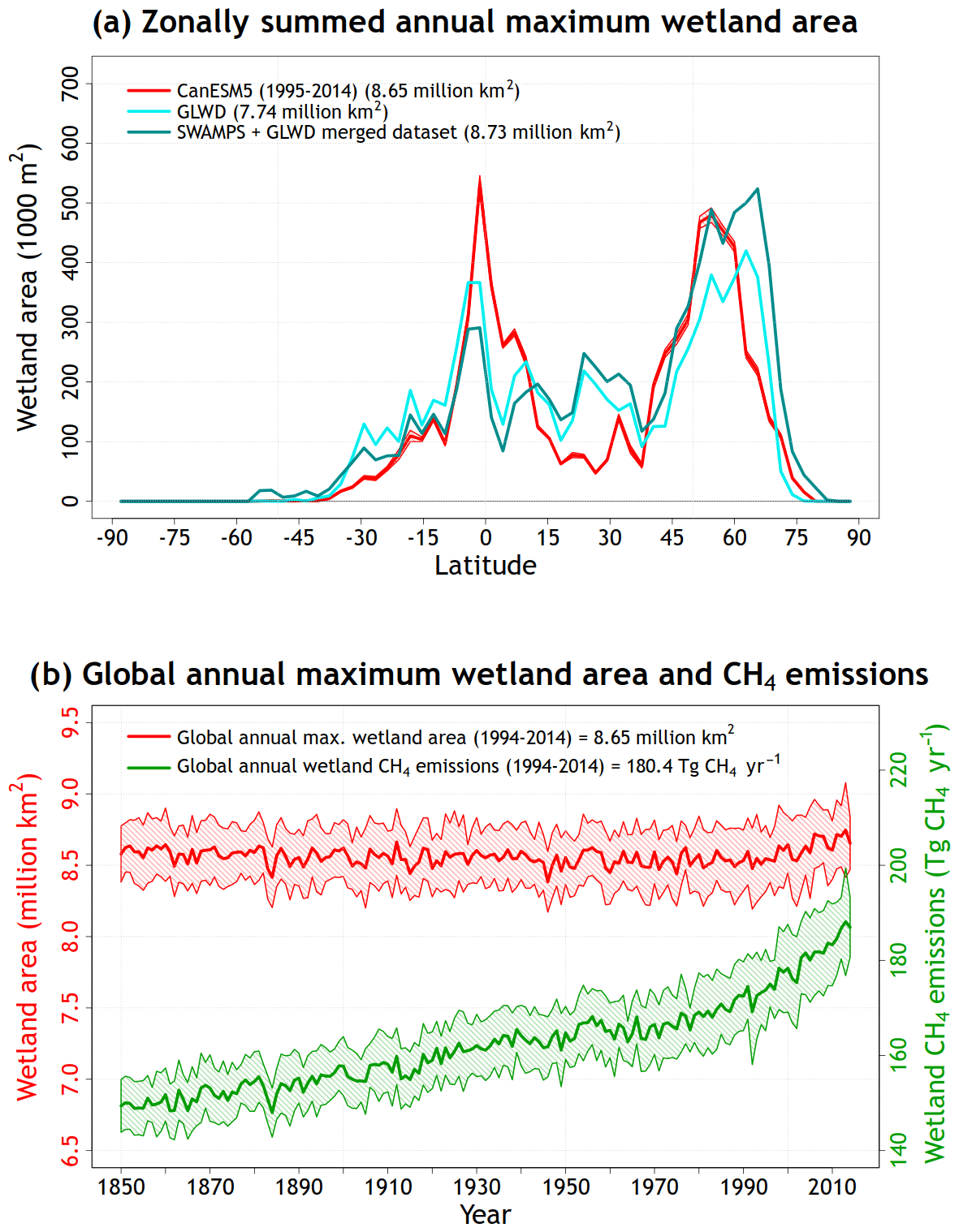
Figure G1 Comparison of simulated zonally summed annual maximum wetland area with observation-based estimates based on the Global Lakes and Wetland (GLWD; Lehner and Döll, 2004) and a new product that is formed by merging remote-sensing-based observations of daily surface inundation from the Surface Water Microwave Product Series (SWAMPS; Schroeder et al., 2015) with the static inventory of wetland area from the GLWD as explained in Poulter et al. (2017) (a). Panel (b) shows the temporal evolution of simulated global annual maximum wetland extent and wetland methane emissions over the 1850–2014 period of the historical simulation.

Figure G1a compares the zonally summed annual maximum wetland area with observation-based estimates based on the Global Lakes and Wetland (GLWD; Lehner and Döll, 2004) and the new product formed by merging remote-sensing-based observations of daily surface inundation from the Surface Water Microwave Product Series (SWAMPS; Schroeder et al., 2015) with the static inventory of wetland area from the GLWD from Poulter et al. (2017). Maximum wetland fraction from the model (1995–2014) and SWAMPS and GLWD (2000–2012) product is calculated as the maximum of 12 monthly mean values for the time period noted and the multiplied by area of the grid cells to calculate zonally summed area. The model overall captures the broad latitudinal distribution of wetlands with higher wetland area in the tropics and at northern high latitudes. The model yields higher wetland area in the tropics than both observation-based estimates due to higher wetland area simulated in the Amazonian region. The Amazonian region is densely forested and the SWAMPS product is unable to map wetlands beneath closed forest canopies. Biases also likely exist in the GLWD dataset since parts of the Amazonian region are fairly remote. The global annual maximum wetland extent of 8.65 million km² also compares well with observation-based estimates of 7.74 (GLWD) and 8.73 (SWAMPS + GLWD) million km².

Figure G1b shows the time evolution of simulated annual maximum wetland extent and wetland methane emissions over the 1850–2014 period from the historical simulation. The shaded range represents the standard deviation over the 25 ensemble members of the historical simulation. While the simulated wetland extent does not change significantly over time, the methane emissions increase from about 150 Tg CH₄ yr⁻¹ during the early pre-industrial period to about 180 Tg CH₄ yr⁻¹ for the present day (1995–2014). This increase in wetland methane emissions is caused by increased vegetation productivity driven by increased atmospheric CO₂ concentration over the historical period. The simulated present-day wetland methane emissions of 180 Tg CH₄ yr⁻¹ are comparable to central estimate of 166 Tg CH₄ yr⁻¹ from Saunois et al. (2016) and their range of 125–204 Tg CH₄ yr⁻¹.