the Creative Commons Attribution 4.0 License.
the Creative Commons Attribution 4.0 License.
 | 08 Nov 2019
Update and evaluation of the ozone dry deposition in Oslo CTM3 v1.0
Amund Søvde Haslerud
High concentrations of ozone in ambient air are hazardous not only to humans but to the ecosystem in general. The impact of ozone damage on vegetation and agricultural plants in combination with advancing climate change may affect food security in the future. While the future scenarios in themselves are uncertain, there are limiting factors constraining the accuracy of surface ozone modeling also at present: the distribution and amount of ozone precursors and ozone-depleting substances, the stratosphere–troposphere exchange, as well as scavenging processes. Removal of any substance through gravitational settling or by uptake by plants and soil is referred to as dry deposition. The process of dry deposition is important for predicting surface ozone concentrations and understanding the observed amount and increase of tropospheric background ozone. The conceptual dry deposition velocities are calculated following a resistance-analogous approach, wherein aerodynamic, quasi-laminar, and canopy resistance are key components, but these are hard to measure explicitly. We present an update of the dry deposition scheme implemented in Oslo CTM3. We change from a purely empirical dry deposition parameterization to a more process-based one which takes the state of the atmosphere and vegetation into account. We examine the sensitivity of the scheme to various parameters, e.g., the stomatal conductance-based description of the canopy resistance and the choice of ozone surface resistance, and evaluate the resulting modeled ozone dry deposition with respect to observations and multi-model studies. Individual dry deposition velocities are now available for each land surface type and agree generally well with observations. We also estimate the impact on the modeled ozone concentrations at the surface. We show that the global annual total ozone dry deposition decreases with respect to the previous model version (−37 %), leading to an increase in surface ozone of more than 100 % in some regions. While high sensitivity to changes in dry deposition to vegetation is found in the tropics and the Northern Hemisphere, the largest impact on global scales is associated with the choice of prescribed ozone surface resistance over the ocean and deserts.
- Article
(9120 KB) - Full-text XML
-
Supplement
(1914 KB) - BibTeX
- EndNote


Ozone is an important trace gas for all life forms on Earth. Depending on the place of its occurrence, it has either a positive or negative connotation. In the stratosphere, ozone absorbs most of the ultraviolet (UV) light from the Sun within the range of 100–315 nm, thus shielding the Earth's surface from the most harmful UV radiation. In addition, ozone is a potent greenhouse gas in both stratosphere and troposphere. With a radiative forcing of 0.40±0.20 W m−2, it is placed third, only surpassed by CO2 and CH4 (IPCC – Intergovernmental Panel on Climate Change, 2013, chap. 8).
In the troposphere, and in particular in ambient air, ozone is considered a highly toxic pollutant. Since the industrial revolution, tropospheric background ozone concentrations have been increasing in the Northern Hemisphere (IPCC – Intergovernmental Panel on Climate Change, 2013, chap. 2). In recent years, the number of episodes of peak concentrations has been, in general, decreasing in North America and Europe due to the implementation of air quality regulations (e.g., Fleming et al., 2018; Mills et al., 2018). At the same time, fast-developing countries, e.g., China or India, saw a significant increase in ozone-related air pollution. Continuously high concentrations of ambient air ozone are hazardous to the whole ecosystem. It is estimated that ozone is cause to an increase in premature deaths (WHO – World Health Organization, 2008), an average global loss of yield in the four major crops (wheat, rice, maize, and soybean) of about 3 %–15 % (Ainsworth, 2017), as well as 7 % loss in primary production in forestry (Wittig et al., 2009; Matyssek et al., 2012). The impact of ozone damage on vegetation and agricultural plants may affect food security in the future especially in Asia (Tang et al., 2013; Tai et al., 2014; Chuwah et al., 2015; Mills et al., 2018) and might be an important additional feedback to climate change (Sitch et al., 2007).
Elevated ozone levels at a site may originate from both the local production of ozone from its precursors, which are transported, and from advection of ozone itself. Long-range ozone transport occurs regularly and might be most important in regions that otherwise lack precursors. Tropospheric ozone is produced in complex photochemical cycles involving precursor gases such as carbon monoxide (CO) or volatile organic substances (VOCs – also known as hydrocarbons) in the presents of nitrogen oxides (NOx). A typical reaction mechanism for CO is sketched in the following. In a sequence of rapid reactions, a peroxyl radical is formed through an initial reaction of CO with a hydroxyl radical •OH. Via a reaction between and NO, NO2 is formed, which is then photolyzed. The resulting atomic oxygen reacts then with O2 (and also under the presence of available co-reactants) to form an ozone molecule. Such a cycle leads to a net production via
Similar cycles involving VOCs exist (Monks et al., 2015). Another source of tropospheric ozone is downward transport from the stratosphere via stratosphere–troposphere exchange (STE) (WMO – Global Ozone Research and Monitoring Project, 2014). Based on observations, STE might only amount to 10 % (550±140 Tg a−1) of the total global ozone budget in the troposphere, while ozone from chemical production is estimated to be 5000 Tg a−1 (Monks et al., 2015). Ozone is removed from the atmosphere by photochemical reactions or scavenging processes. Major sinks are photolysis followed by a reaction with water vapor to form OH, reactions with HO2, titration reactions, and dry deposition. We will come back to the latter later in this section and cover the implemented scheme in more detail in Sect. 2.1.
Since ozone is highly reactive, its global mean lifetime in the troposphere is roughly 22 d but ranges from a few days in the tropical boundary layer up to 1 year in the upper troposphere (Stevenson et al., 2005; Young et al., 2013). The abundance of tropospheric ozone therefore varies, e.g., with the time of day, season, altitude, location (Schnell et al., 2015), or weather conditions in general (Otero et al., 2018). Typical concentrations of surface ozone range from 10 ppb over the tropical Pacific to 100 ppb in the downwind areas of highly emitting sources (IPCC – Intergovernmental Panel on Climate Change, 2013, chap. 8). This variability poses a challenge for both trend analysis from observations as well as validation and intercomparison of models. From the observational side, the number of long-term observations (starting before the 1950s) is limited and restricted to mainly European sites. Most of these have indicated a doubling of tropospheric ozone since the 1950s (IPCC – Intergovernmental Panel on Climate Change, 2013, chap. 2). But especially the very low pre-industrial ozone abundance cannot be reproduced by the likes of most models. These early observations, however, were subject to interference by other species, e.g., SO2. Among the participating models in the Atmospheric Chemistry and Climate Model Intercomparison Project (ACCMIP), there is a general tendency to underestimate tropospheric ozone burden (e.g., 10 %–20 % negative bias at 250 hPa in the Southern Hemisphere (SH) tropical region) (IPCC – Intergovernmental Panel on Climate Change, 2013, chap. 8). With respect to surface ozone, Schnell et al. (2015) conclude that all ACCMIP models, which reported hourly surface ozone, tend to overestimate surface ozone values in North America and Europe in comparison with available observations. A key to fathom these slightly contradicting results may lie in the used dry deposition schemes.
Removal of any substance from the atmosphere which is not involving rain, e.g., through gravitational settling or by uptake by plants, soil, and water, is referred to as dry deposition. The process of dry deposition is important for predicting surface ozone concentrations and understanding the observed amount and increase of tropospheric background ozone. It is estimated that 1000±200 Tg a−1 of ozone are removed from the atmosphere by dry deposition processes (Monks et al., 2015). A newer study by Luhar et al. (2018), however, indicates much lower amounts (722.8±87.3 Tg a−1) due to lower dry deposition to the oceans. Conceptually, dry deposition is a product between near-surface ozone concentration [O3](z0) (e.g., the lowermost model level) and a dry deposition velocity . Species-dependent dry deposition velocities , which are synonymously referred to as conductance Gi, for any gaseous species i, are typically calculated following a resistance-analogous approach:
wherein aerodynamic Ra, quasi-laminar layer , and canopy resistance are key components (Wesely, 1989; Seinfeld and Pandis, 2006). For all gases, Ra is the same, while and vary from gas to gas and also depend on land surface types (e.g., ice/snow, water, urban, desert, agricultural land, deciduous forest, coniferous forest). Originally, Wesely (1989) used fixed seasonal average dry deposition resistance for each land surface type. For all three types of resistance in this Wesely-type parameterization, more process-oriented formulations have been developed and validated over the years. Luhar et al. (2017) have validated ozone dry deposition to the ocean with respect to three different formulations of surface resistance. Based on the global atmospheric composition reanalysis performed in the ECMWF project Monitoring Atmospheric Composition and Climate (MACC) (MACC-II Consortium, 2011) and a more realistic process-based oceanic deposition scheme, Luhar et al. (2018) found that the ozone dry deposition to oceans amounts to 98.4±30.0 Tg a−1. In particular, Luhar et al. (2018) found that the average surface resistance of ozone over the ocean (rc=2200 s m−1) is highly overestimated in most models. An update on the ozone surface resistance over snow- and ice-covered surfaces has been provided from combined model and observation studies (Helmig et al., 2007, m s−1). Canopy conductance is parameterized at the single-leaf level (stomatal conductance) for various plant function types (PFTs) as well as for single plant species based on empirical studies (Jarvis, 1976; Ball et al., 1987; Simpson et al., 2012; Mills et al., 2017). But progress has also been made on process-oriented modeling of stomatal conductance (Anderson et al., 2000; Buckley, 2017). The variety of differing formulations and choices of parameters leads to a wide spread of results in model intercomparisons (Hardacre et al., 2015; Derwent et al., 2018) and about 20 % uncertainty on the resulting total dry deposition (Monks et al., 2015).
In Sect. 2, we will briefly describe Oslo CTM3, give a detailed account of the new dry deposition scheme (Sect. 2.1) as well as present pre-processing of meteorological input data to compute necessary input to the dry deposition scheme such as the beginning and duration of the greening season (GDAY, GLEN) and photosynthetic photon flux density (PPFD) (Sect. 2.2). In Sect. 3, we present sensitivity tests with respect to manifold parameters in the dry deposition scheme (Sect. 3.1) and validate our results with respect to results from the multi-model intercomparison of Hardacre et al. (2015) (Sect. 3.2), the MACC reanalysis (Sect. 3.3), and to surface ozone observations (Sect. 3.4). In Sect. 4, we will summarize and discuss our results and draw conclusions for further development of the model.
Oslo CTM3 is an offline, three-dimensional global chemistry transport model (CTM). The key components of Oslo CTM3 have been described and evaluated by Søvde et al. (2012). A detailed account of the capabilities of Oslo CTM3 in simulating anthropogenic aerosol forcing in the past and recent past using the Community Emission Data System (CEDS) historical emission inventory (Hoesly et al., 2018) is given by Lund et al. (2018). Oslo CTM3 can also be coupled to the Model of Emissions of Gases and Aerosols from Nature (MEGAN v2.10) (Guenther et al., 2006). A publication focusing on this is planned.
While the meteorological data driving Oslo CTM3 are given at a resolution of T159N80L60, with the highest model level at 0.02 hPa, it is very time and memory consuming to run Oslo CTM3 with full chemistry at this resolution. Therefore, we reduced the horizontal resolution to in our experiments. In the following, we will give a detailed account of the new dry deposition scheme and the equations that we use.
2.1 Ozone dry deposition scheme
In the original dry deposition scheme, the state of the atmosphere was not taken into account. Dry deposition velocities were rather parameterized following the work of Wesely (1989) with parameter updates from Hough (1991). This means that seasonal day and night average deposition velocities for different land surface types (water, forest, grass, tundra/desert, and ice and snow) were in use. Day was distinguished from night by solar zenith angles below 90∘. Winter was defined by temperatures below 273.15 K for grid boxes containing land masses. For ocean, winter and summer parameters are equal in this parameterization; therefore, no distinctive treatment was needed for ocean grid boxes. In addition, a reduced uptake due to snow cover above 1 m for forest and 10 cm for grass/tundra, respectively, was taken into account. We will refer to this parameterization as the “Wesely scheme”.
Regarding the new dry deposition scheme, we mainly follow Simpson et al. (2012) in their description of dry deposition used in the European Monitoring and Evaluation Programme (EMEP) MSC-W model (see also Emberson et al., 2000; Simpson et al., 2003; Tuovinen et al., 2004), which is used for air quality modeling implementing the Convention on Long-Range Transboundary Air Pollution (CLRTAP). We will refer to the new scheme as the “mOSaic scheme” throughout the rest of the paper. The mOSaic scheme is a more physical approach compared to the previously used Wesely scheme, because it takes state (e.g., pressure, temperature) of the atmosphere as well as dynamics (e.g., wind stress) of the boundary layer into account. To a certain degree, the global variety of plants and their variability throughout the seasons is also acknowledged. The mOSaic scheme is implemented for the gaseous species O3, H2O2, NO2, PAN, SO2, NH3, HCHO, and CH3CHO. Since CO has a very small uptake and is not included in Simpson et al. (2003, 2012), the Wesely parameterization is kept. In addition to the gaseous species, Simpson et al. (2012) also modify aerosol deposition velocities, namely black carbon (BC) and organic carbon (OC), sulfuric aerosols (SO4, MSA), and secondary organic aerosols (SOAs), but we have not updated our model with respect to these.
As displayed in Eq. (1), the dry deposition computation is subdivided into contributions from three different types of resistance. The main idea of a mosaic approach is to calculate these types of resistance separately for each land surface type k in each grid cell: , , and . The grid cell average dry deposition velocity is then defined by weighting each individual by the corresponding land fraction factor fk:
2.1.1 Aerodynamic resistance
In general, the aerodynamic resistance describes the turbulent transport of any substance down to the surface. To derive , we follow Simpson et al. (2003, 2012) and compute a local friction velocity at reference height zref (Eq. 52, Simpson et al., 2012):
with the average wind speed at reference height, the Kármán constant κ=0.40, the integrated stability equation for momentum Ψm (e.g., Garratt, 1992), a grid average Obukhov length L, displacement height dk, and roughness length (, for forests, , for vegetation other than forests). Taking the height of vegetation into consideration, we have chosen the model level such that m. Using the derived from Eq. (3), a local Obukhov length Lk can be obtained from (Eq. 8, Simpson et al., 2012):
Herein, H is the sensible heat flux, g is the standard gravitational acceleration, cp the specific heat capacity, and T2 m the 2 m temperature. With these, we can compute the aerodynamical resistance for each land surface type (Eq. 8.8, Simpson et al., 2003):
with the integrated stability equation for heat Ψh (e.g., Garratt, 1992). Both integrated stability functions (Ψm, Ψh) and corresponding parameters are listed in Sect. S1 in the Supplement.
2.1.2 Quasi-laminar layer resistance
The quasi-laminar layer resistance is species specific and differs over land and ocean surfaces. Over land, we use (Eq. 53, Simpson et al., 2012)
wherein Pr is the Prandtl number (0.72 for air and other gases) and Sci is the Schmidt number for a gas i. Equation (6) differs from a similar formulation in Seinfeld and Pandis (2006) by a factor of roughly 1.25. From , with the kinematic viscosity of air ν, we derive a Schmidt number in water equivalent:
with the molecular diffusivity for any gas Di, the Schmidt number of water () and its molecular diffusivity ( m2 s−1). The used ratios are taken from Simpson et al. (2012, Table S18). Over the ocean, we use (Eq. 54, Simpson et al., 2012)
with an imposed lower threshold of 10 s m−1 and an upper limit of 1000 s m−1. The computation of roughness length z0 over the ocean is divided into a calm and a rough sea case, with a threshold of 3 m s−1. For calm sea, we apply the following upper limit (Hinze, 1975; Garratt, 1992, with a slightly higher coefficient of 0.135):
The kinematic viscosity of air ν herein can be computed from
For the temperature-dependent dynamic viscosity of air μ(T), we chose a linear fit to Sutherland's law through the origin within the temperature range : . But despite its rough accuracy, we found that the choice of μ(T) has no effect on (Sect. S2, Figs. S1–S2). In Eq. (10), ρ is substituted by the air density using the ideal gas law. P0 is the surface pressure, as T the 2 m temperature is chosen, and Rair is the universal gas constant for air. The rough sea case follows the method of Charnock (1955) and Wu (1980):
with a gravitational acceleration g=9.836 m s−2. The allowed maximum roughness length in both cases is set to 2 mm. Since the z0 values computed with this parameterization are rather small (, m), is set to its lower limit of 10 s m−1 in about 91 % of all cases (see Sect. S2, Fig. S3).
2.1.3 Surface resistance
The surface resistance consists of both stomatal and non-stomatal resistance.
The stomatal conductance is a measure of the rate of CO2 exchange and evapotranspiration through the stomata of a leaf. There are several environmental conditions affecting the opening and closing of the stomata and hence the capability of respiration (e.g., light, available water). Stomata sluggishness, a state in which the stomata can no longer fully close, has been reported as ozone-induced damage (Hoshika et al., 2015) but is not taken into account in our formulation. To reflect part of the underlying mechanism, the leaf-level molar stomatal conductance in the mOSaic scheme is computed using a common multiplicative ansatz (Ball et al., 1987; Mills et al., 2017):
The factors herein are normalized and vary within the range 0–1. They account for leaf phenology (fphen), light (flight), temperature (fT), water vapor pressure deficit (fD), and soil water content (fSW). All factors differ with land use type k. For clarity reasons, we drop this index in the following, as long as it is not necessary for the equation's completeness. The maximum molar stomatal conductance is given by , which is in units of . A unit conversion to m s−1 is necessary in our model:
Herein, R is the universal gas constant. To annotate the differing units, we use the index “m” in Eq. (12). The temperature adjustment fT is computed from
with . The parameters Tmin, Tmax, and Topt are tabulated for various plant functional types. All parameters are taken from Simpson et al. (2012, Tables S16, S19). Since fT turns negative outside the range defined by Tmin, Tmax, we impose a lower limit of 0.01 for numerical reasons.
The water vapor deficit (VPD) is proportional to the saturation partial pressure of water () and relative humidity (RH):
Using tabulated values of fmin, Dmin, and Dmax, the water vapor pressure deficit penalty factor fD can be computed:
The penalty factor with respect to available soil water (SW) fSW is defined as
SW is evaluated at a soil depths of 0.28–1 m, which corresponds to SWVL3 in OpenIFS.
The phenology of a plant typically describes its life cycle throughout a year; e.g., at midlatitudes and for deciduous species, it starts with the emergence of leaves in spring and ends in fall. In the mOSaic scheme, phenology is parameterized with respect to the start of the greening season (SGS) and its end (EGS). Details about our treatment of these are given in Sect. 2.2.1. In summary, our adaption of the fphen parameterization reads as follows:
Herein, we use the SGS- and EGS-derived parameters: day of greening season (GDAY), the time elapsed starting at the SGS, and the total length of the greening season (GLEN), the time span between EGS and SGS. The parameters ϕa, ϕb, ϕc, and ϕd define start or end points in the five phases of phenology in the mOSaic scheme, while ϕe, ϕf, ϕAS, and ϕAE control the temporal timing (Fig. 1). If GLEN is zero, we are, e.g., in Arctic regions, and there is no vegetation anyway; therefore, fphen=0. Before the start of the greening season (GDAY=0), fphen=0. Since this phenology is tuned to Northern Hemisphere (NH) midlatitudes, it does not apply to the tropics. We therefore decided to set fphen=1 if GLEN is greater than or equal to 365, which is the case in the tropics.
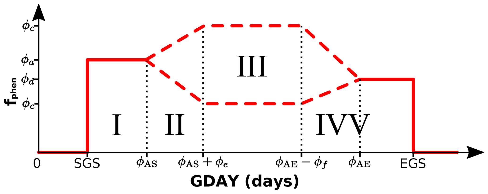
Figure 1Sketch of the five different phases in plant phenology fphen in accordance with Eq. (18).
Light in the wavelength band 400–700 nm to which the plant chlorophyll is sensitive is called photosynthetic active radiation (PAR). The integral of PAR over these wavelengths is the photosynthetic photon flux density (PPFD). The correction factor flight in response to varying PPFD is
In the mOSaic scheme, non-stomatal conductance is explicitly calculated for O3, SO2, HNO3, and NH3. For all other species, an interpolation between O3 and SO2 values is carried out. The non-stomatal conductance for O3 consists of two terms: one depending on vegetation type and one depending on the soil/surface. For each land surface type k, we can write
SAIk is the surface area index for vegetation type k, which is leaf area index (LAI) plus a value that represents cuticles and other surfaces. The external leaf resistance is defined by
Herein, FT is a temperature correction factor for temperatures below and :
θ2 m is the 2 m temperature in ∘C. For most land surface types, SAI≡LAI. Some exceptions are
Extending the mOSaic scheme to the Southern Hemisphere, we use the growing season for crops defined in Table 1.
Table 1Definition of growing season for crops used in Oslo CTM3 in the NH and SH.

In this way, vegetation affects the conductance also by being there, not only by uptake through the stomata. The in-canopy resistance Rinc (Erisman et al., 1994) is then modified with respect to each (vegetated) land surface type in k:
where hk(lat) is the latitude-dependent vegetation height (see explanation at the end of this section) and b=14 m−1 is an empirical constant. The canopy resistance described in Simpson et al. (2012) does not take temperature and snow into account and is zero for non-vegetated surfaces, but we will adopt the correction previously used in the Oslo CTM3 Wesely scheme.
As initially mentioned, the necessary depth of snow to cover a certain type of vegetation differs. Therefore, we calculate a snow cover fraction fsnow using the snow depth SD, which is available in units of meters of water equivalent from the meteorological input data, scaled to 10 % of the vegetation height. is tabulated. We correct for temperature by FT and for snow cover fraction:
The bulk canopy conductance is then defined as
wherein LAI is the one-sided leaf area index taken from ISLSCP2 FASIR, gsto the leaf-level stomatal conductance, and Gns the bulk non-stomatal conductance.
2.1.4 Latitude-dependent vegetation height
The vegetation height hk(lat) as described by Simpson et al. (2012) is linearly decreasing with latitude between 60 and 74∘ N. To adapt this to a global model, we made a few additional assumptions. The tabulated height for each vegetation type hk in the mOSaic scheme is regarded as constant at midlatitudes (40–60∘). Towards the poles, we decrease the height of each vegetation type using the same rate as described in Simpson et al. (2012). At a latitude of 74∘, a minimum height of is reached and kept constant. Towards the Equator, we increase the height linearly so that at a latitude of 10∘ a maximum height of 2⋅hk is reached which is then held constant. We also assume symmetry in both hemispheres. Presuming a typical tree height of 20 m at midlatitudes, this stepwise function yields a height of 8 m at high latitudes and 40 m in the tropics, which is not unrealistic. For four example PFTs, results are shown in the Supplement (Sect. S3, Fig. S4).
2.1.5 Mapping of land surface types
Oslo CTM3 is configured to read land surface types from either the ISLSCP2 (https://daac.ornl.gov/cgi-bin/dataset_lister.pl?p=29, last access: 20 November 2017) product from MODIS or Community Land Model (CLM; http://www.cgd.ucar.edu/tss/clm/, last access: 7 November 2017) 2 categories, which have to be mapped to the land surface types used in the mOSaic scheme (Fig. 2). For both MODIS and CLM 2 land surface categories, snow and ice cover is estimated from input meteorology, while is defined as . From the MODIS category “barren or sparsely vegetated”, everything poleward from 60∘ is defined as tundra, while everything equatorward is categorized as desert. This mapping differs from the one used in the Wesely scheme.

Figure 2Mapping of land surface categories. Either land surface categories from ISLSCP2 product of MODIS or the Community Land Model (CLM) 2 can be chosen for mapping to the land surface types we use in the mOSaic scheme. Water bodies of MODIS are actually not mapped. For both MODIS and CLM 2 land surface categories, snow and ice cover is estimated from input meteorology, while water is defined as . From the MODIS category “barren or sparsely vegetated”, everything poleward from 60∘ is defined as tundra, while everything equatorward is categorized as desert.
2.2 Pre-processing
As mentioned in the previous section, there are two variables needed for computing the stomatal conductance which are not directly available from the meteorological input data: the greening season, as the time of the year in the mid- and high latitudes when it is most likely for plants to grow, and the photosynthetic photon flux density, as the amount of light that plants need to photosynthesize. In the following, we present the necessary pre-processing of the variables. It is planned to implement an online computation of these variables into Oslo CTM3 later on.
2.2.1 Greening season
In Eqs. (20)–(23), Simpson et al. (2012) use prescribed start of growing season (SGS) and end of growing season (EGS) at 50∘ N (dSGS, dEGS), together with lapse rates (∇dSGS, ∇dEGS) to define phenology and dry deposition over agricultural areas. For the growing season of crops in the computation of non-stomatal conductance, we use also prescribed values (Table 1), while for the stomatal conductance, as shown in Eq. (18), we use the SGS- and EGS-derived parameters: GDAY, the time elapsed starting at the SGS, and the total length of the greening season (GLEN), the time span between EGS and SGS. Since the parameterization of SGS and EGS in Simpson et al. (2012) is not applicable in a global model, another latitude-dependent parameterization is needed. First, we used a parameterization which was already implemented in Oslo CTM3 and which had been adopted from the Sparse Matrix Operational Kernel Emissions – Biogenic Emission Inventory System (SMOKE-BEIS; https://www.epa.gov/air-emissions-modeling/biogenic-emission-inventory-system-beis, last access: 24 October 2018). SMOKE-BEIS has fixed values for SGS and EGS for all regions but NH midlatitudes (23∘ < lat < 65∘), where it uses lapse rates of ∇dSGS=4.5 and ∇dEGS=3.3. As this parameterization is optimized for North America, it does not work well in Europe, e.g., most of northern Scandinavia has no allocated vegetation period. This basically results in a suppression of canopy resistance in northern Scandinavia.
In agriculture, there are different empirical rules to estimate the SGS and EGS. The simplest assumption is that greening starts after 5 consecutive days with a daily average temperature above 5 ∘C, and vice versa for EGS. Other estimates use growing degree days (Levis and Bonan, 2004; Fu et al., 2014a), include soil moisture (Fu et al., 2014b), or rely on satellite observations. A comprehensive evaluation of different techniques is given by Anav et al. (2017). Another solution would be the usage of a proper land surface model, e.g., LPJ-GUESS, CLM, but the integration of such models into Oslo CTM3 is not planned at the moment.
Based on the empirical rule (5 ∘C days), we have pre-processed our meteorological input data offline. We added some additional criteria to prevent “false spring”: if, within these 5 d, the average temperature drops below or rises above 5 ∘C, the counter is reset, respectively. First, we used the 5 ∘C day criteria for 45∘ < lat < 85∘ in the NH but extended them also to 35∘ < lat < 65∘ in the SH. In all other cases and where the 5 ∘C day criteria fail, we still use the SMOKE-BEIS parameterization. The described algorithm written in Python 2.7 has been included in Sect. S4. An example map of the computed GLEN using the 5 ∘C day criteria in both hemispheres is shown in Fig. 3.
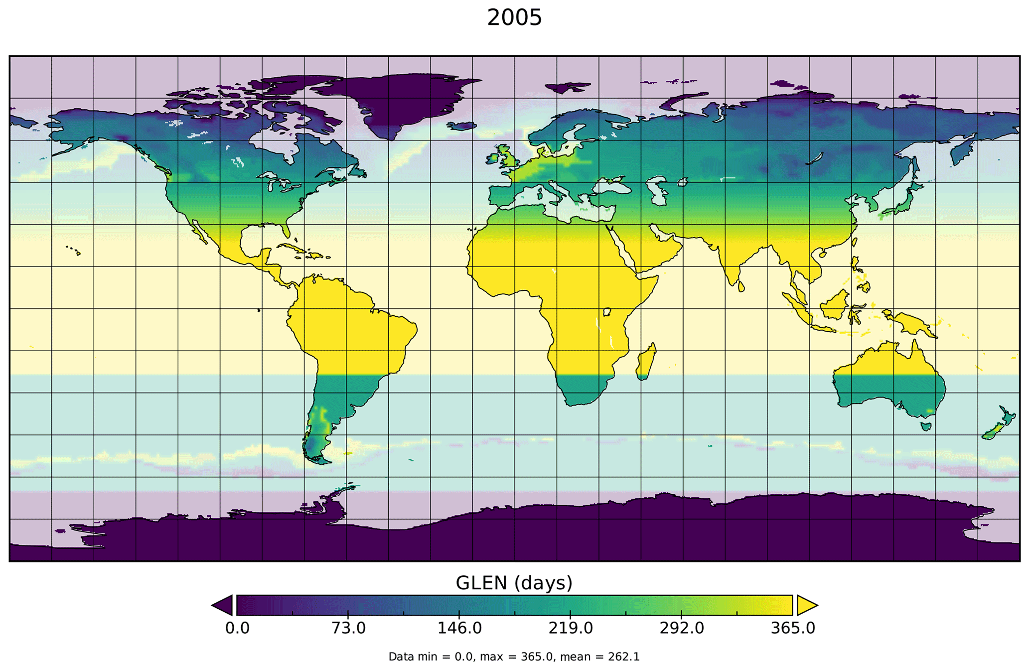
Figure 3Pre-processing of greening season from meteorological surface temperature fields. Shown is the total length of the greening season (GLEN) for the year 2005. The 5 ∘C day criteria have been used in both hemispheres' mid–high latitudes. Ocean has been shaded to indicate that greening season will only affect land.
2.2.2 Photosynthetic photon flux density
From OpenIFS an accumulated surface PAR is available. It is integrated both spectrally (presumably 400–700 nm) and temporally. For practical use in Eq. (19), we de-accumulate this field with respect to time and refer to the result as PPFD.
The main obstacle is that PAR has been accumulated since model start, so that the first field kept from the original OpenIFS simulation (00:00 UTC) is 12 h after model start (12:00 UTC on the previous day). In other words, the first time step of each day in Oslo CTM3 has already accumulated PAR from 12:00 UTC on the previous day. De-accumulation of time 03:00 to 21:00 UTC simply means computing the difference:
For de-accumulation of the remaining time step, the best choice is subtracting the difference between 21:00 and 12:00 UTC of the previous day:
and limit the result to positive values only. An example PAR de-accumulation for 2 January 2005 is shown in Sect. S5 (Figs. S5–S7). The resulting PPFD fields are still accumulated over a time period of 3 h and should be divided by 3. A known issue (see https://confluence.ecmwf.int/display/CKB/ERA-Interim+known+issues, last access: 29 October 2019) in the OpenIFS (cycles ≤ c41r2) causes surface PAR values to be about 30 % below observations. To counter this, we decided to refrain from the division at this stage but need to bear this in mind for later OpenIFS cycles.
In this section, we present results from manifold Oslo CTM3 model integrations testing different parameters of the mOSaic scheme. We focus on changes in ozone total dry deposition , dry deposition velocities , concentrations in the lowermost model level [O3](p0), and tropospheric burden ∑tropO3. We evaluate our results with respect to the multi-model comparison of ozone dry deposition by Hardacre et al. (2015) (Sect. 3.2), the MACC reanalysis (Sect. 3.3), and observations (Sect. 3.4). Oslo CTM3 is driven by meteorological input fields from ECMWF – OpenIFS cy38r1 (https://www.ecmwf.int/en/forecasts/documentation-and-support/evolution-ifs/cycle-38r1-summary-changes, last access: 4 October 2018). The CEDS historical emission inventory (Hoesly et al., 2018) is used for anthropogenic emissions, while biomass burning is covered in daily resolution by NASA's Global Fire Emissions Database version 4 (GFEDv4, Randerson et al., 2018). Biogenic emissions are taken from MEGAN-MACC output (Sindelarova et al., 2014), while emissions from soil and wetlands are computed by MEGAN. Resultant NOx emissions are upscaled to match the Global Emissions InitiAtive (GEIA) inventory and are estimated to amount to 6.55 Tg (N) a−1. For oceanic emissions of CO, we use predefined global fields from POET (GEIA-ACCENT emission data portal, 2003). Emissions of CH4 are taken from the EU project (EU GOCE 037048) “Hydrogen, Methane and Nitrous oxide: Trend variability, budgets and interactions with the biosphere (HYMN)” for the year 2003 and scaled to oceanic amounts of CH4 from NASA. In the following (Sect. 3.1), we will present the various model sensitivity studies.
3.1 Sensitivity studies
Due to significant differences between the mOSaic scheme and the previous Wesely scheme with respect to implementation, it is not possible to fully disentangle and trace back every single difference in results to a respective change. Therefore, we conducted one reference simulation denoted as mOSaic and in total seven sensitivity studies to probe the parameter space for stomatal conductance (mOSaic_offLight, mOSaic_offPhen, and mOSaic_SWVL1), ozone surface resistance (mOSaic_ice, mOSaic_desert, and mOSaic_hough), and emissions (mOSaic_emis2014). A reference simulation featuring the Oslo CTM3 Wesely scheme has been conducted and will be referred to as Wesely_type, indicating that other implementations of the original work by Wesely (1989) may exist in other models. All model experiments discussed in the following are summarized in Table 2. An “x” therein denotes that the model was run exactly in the configuration and with parameters as has been described in Sect. 2. For all model integrations, the meteorological reference year is 2005. This choice affects the direct comparison with data and studies that either show results based on decadal averages or differing years, because non-linearities in ozone formation and destruction make ozone concentrations sensitive to both differences in local concentration of precursors and meteorological conditions (Jin et al., 2013).
First, we take a closer look at the influence of certain parameters on the stomatal conductance. As indicated by the names, mOSaic_offLight and mOSaic_offPhen are rather extreme scenarios completely switching off the sensitivity to light and phenology in Eq. (12) by setting flight and fphen to a fixed value of 1, respectively. Because of the underlying research project's focus on Arctic and alpine ecosystems, where water might only be available from upper soil layers, an experiment was conducted using the uppermost soil water level (SWVL1) in the implementation of fSW. After this, we want to confirm the importance of choice of for different land surface types. We conducted three experiments looking at a update (Helmig et al., 2007) (mOSaic_ice), observed (Güsten et al., 1996) (mOSaic_desert), and an approximation of originally used in Wesely_type (Wesely, 1989; Hough, 1991). Finally, we run a simulation with emissions for the year 2014 instead of 2005 (EMEP_emis2014) to characterize the general influence of differing emissions on ozone.
Wesely (1989); Hough (1991)Simpson et al. (2012)Simpson et al. (2012)Simpson et al. (2012)Simpson et al. (2012)Simpson et al. (2012)Helmig et al. (2007)Simpson et al. (2012)Güsten et al. (1996)Simpson et al. (2012)Wesely (1989)Hough (1991)Table 2Summary of specifications of all simulations discussed in this section. For simplicity, only the tested parameters are listed. An “x” denotes that the model was run exactly in the configuration as has been described in Sect. 2. Here, “n/a” means that these parameters are not applicable in this experiment for it has been conducted with Wesely scheme.
a s m−1. b s m−1. c For adapted values, see Sect. S6.
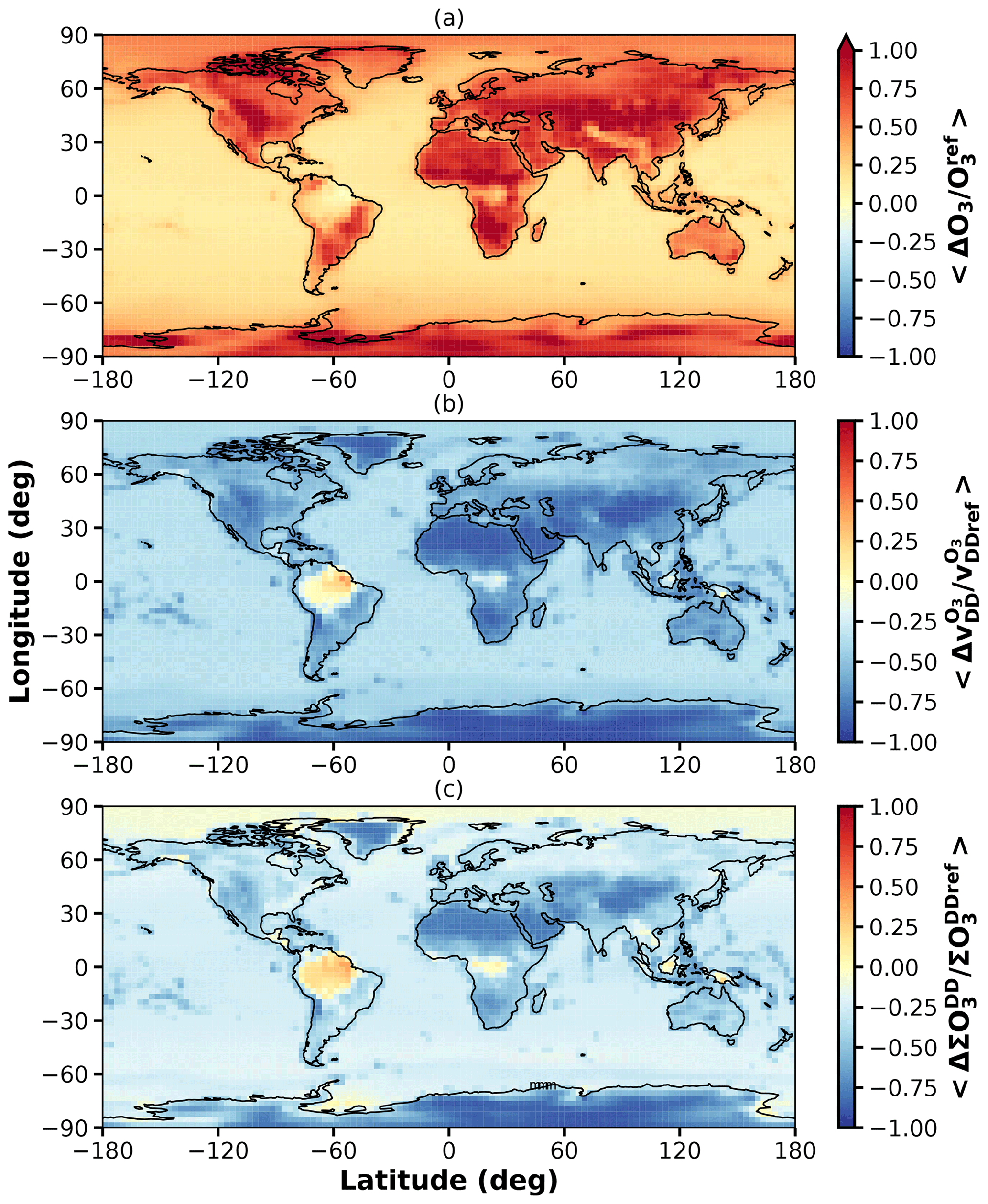
Figure 4Relative difference between reference simulations mOSaic and the Wesely_type with respect to (a) average surface ozone; (b) average ozone dry deposition velocity; (c) total amount of ozone removed from the atmosphere by dry deposition.
In Fig. 4, we show global distributions of the relative difference between mOSaic and Wesely_type for surface ozone, dry deposition velocity, and total ozone dry deposition. The surface ozone increases globally except for some regions covered by tropical forest. Especially in desert regions in Africa, North America, and Asia, the surface ozone increases by more than 100 %. Consistently, dry deposition velocities decrease globally by the same order of magnitude in these regions, while they increase over tropical forest. With respect to total dry deposition, the picture is a bit less clear. We find a decrease of total dry deposition of ozone in desert regions and ocean-covered areas and an increase in regions covered by tropical forest, while at mid- and high latitudes in both hemispheres only small changes are visible. A possible explanation for this divergence especially in desert regions is the difference between the prescribed surface resistance in the Wesely scheme in comparison to those used in mOSaic. We come back to this in the following sections.
3.2 Comparison with modeling results
In the evaluation of our model, we closely follow suggestions by Hardacre et al. (2015). For the purpose of comparison with the multi-model mean of the Task Force on Hemispheric Transport of Air Pollution (TF HTAP) models, we also have regridded our data to a horizontal resolution of . In Sect. 3.2.1, we look at zonal distributions of [O3](p0), , and for all our sensitivity simulations, and study seasonal cycles of hemispheric ozone, as well as for nine land surface types (Sect. 3.2.2). From this, we estimate the total annual ozone dry deposition onto ocean, ice, and land surfaces and compare this also with results from Luhar et al. (2017).
Dry deposition velocities are directly available only for the new model version. For Wesely_type, monthly averaged dry deposition velocities had to be retrospectively estimated from the ratio between the total ozone dry deposition and monthly averaged ozone amount in the lowermost model level O3(p0):
Herein, , with the monthly average height of the lowermost model level in each grid box Δhmonth and the respective number of seconds in a month smonth. In the case of mOSaic, resulting values for from Eq. (29) are compatible with the values which are directly available from model output.
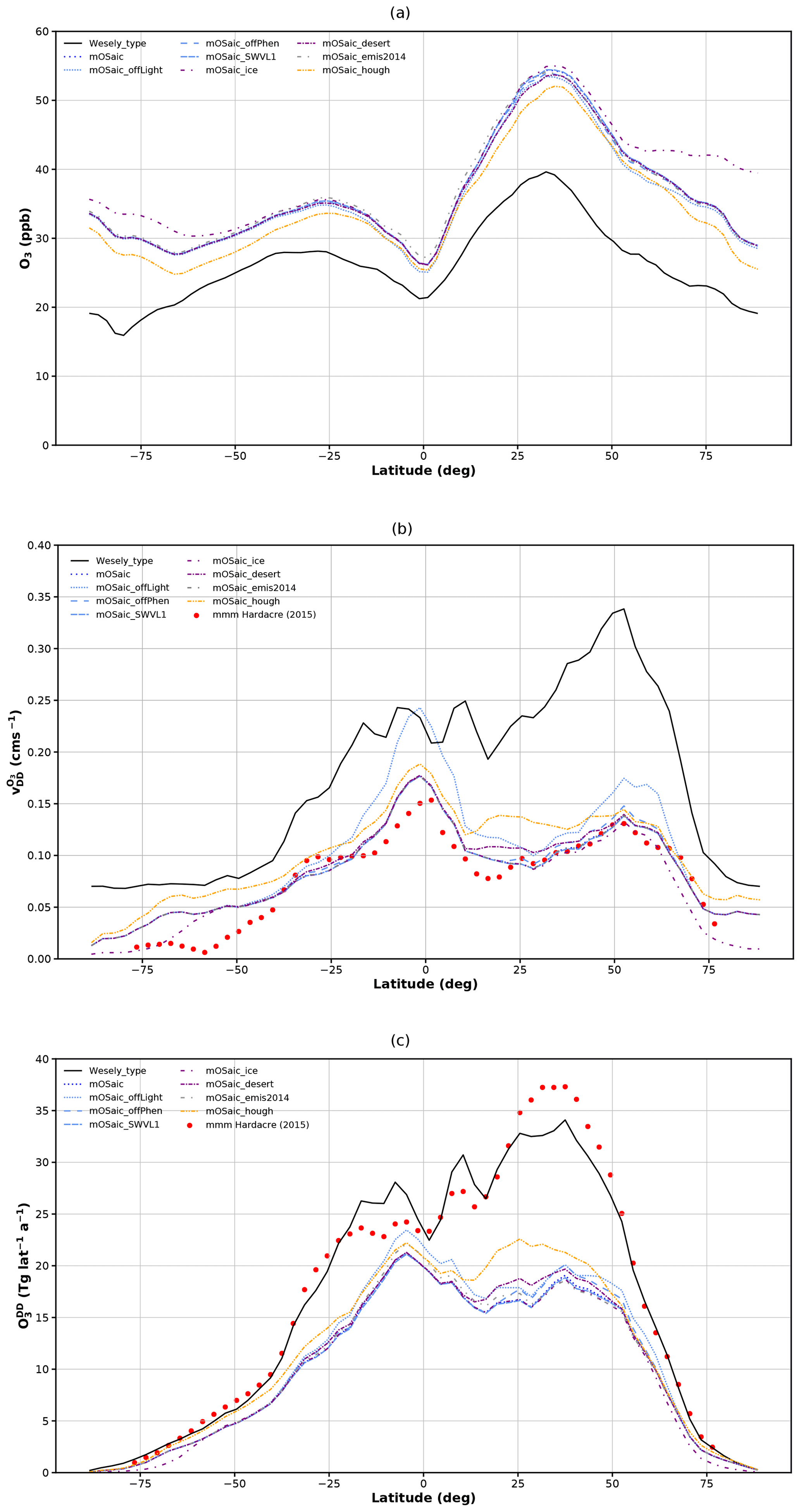
Figure 5Comparison of the manifold Oslo CTM3 integrations with respect to (a) ozone concentrations in the lowermost model level, (b) annual average ozone dry deposition velocity, and (c) total annual ozone dry deposition. The different colors indicate sets of simulation with similar baselines. The multi-model mean from the evaluation of TF HTAP models by Hardacre et al. (2015) is shown as a reference (where available).
3.2.1 Zonal distribution
The annual zonal average with respect to surface ozone concentration (Fig. 5a) displays on average, consistent with Fig. 4a, a global increase of surface ozone concentrations by 6 ppb comparing mOSaic to Wesely_type. This increase is largest in the zonal band 25–50∘ N, which contains the major deserts. In the deep tropics (5∘ S–5∘ N), the increase is smallest (𝒪(5 ppb)). We find that the mOSaic scheme further intensifies the strong asymmetry between the Northern Hemisphere and Southern Hemisphere as a consequence of the distribution of the continental land masses and vegetation thereon. Among the sensitivity studies focusing on the stomatal conductance, there is only a low absolute variance. Neglecting the dependence on light in the stomatal conductance formulation (mOSaic_offLight) – or in other words allowing photosynthesis 24/7 – decreases the ozone concentration by 1–2 ppb in the tropics and NH midlatitudes, while choosing soil water at shallower depths (mOSaic_SWVL1) increases [O3] insignificantly. Rather surprisingly, switching off the phenology completely (mOSaic_offPhen) amounts on average only to a small difference (𝒪(<1 ppb)). Most remarkably, but expected due to the much smaller prescribed dry deposition velocity over ice and snow, mOSaic_ice displays a doubling of surface ozone in the high Arctics compared to Wesely_type (𝒪(20 ppb)) but affects ozone concentrations down to latitudes at about 50∘ in both hemispheres. Reducing by 60 % (mOSaic_desert), a reduction on the order of 1 ppb is found mainly limited to the NH. The largest impact on ozone concentrations (𝒪(2–5 ppb)) is found for the experiment mOSaic_hough which is closest to Wesely_type, since we used on average the same (see Sect. S6). The scenario of differing emissions (2005 in comparison to 2014 or more specifically mOSaic compared to mOSaic_emis2014) yields higher ozone concentrations in the Northern Hemisphere in 2005 in accordance with a reduction in sulfur and NOx emissions in southeast Asia in later years. An opposite tendency is seen for latitudes south of 30∘ N, where an increase in ozone precursors is seen in CEDS.
The are shown in Fig. 5b. The dry deposition velocities in the mOSaic scheme are well below the Wesely scheme and in remarkable agreement with the results shown by Hardacre et al. (2015). In the Arctics, except for mOSaic_ice, all model experiments are slightly above the multi-model mean. This indicates that, with respect to the other models, the Helmig et al. (2007) surface resistance above ice and snow should be considered as the new standard for Oslo CTM3. This may, however, lead to an overcompensation of the current Arctic low bias in surface ozone in Oslo CTM3 and needs further evaluation. The dry deposition velocities are of course independent of the emission scenario but display a strong sensitivity to flight, fphen, and especially the choice of . The shape of the normalized zonal average dry deposition velocities of the mOSaic scheme are more similar to the multi-model mean than to Wesely_type (Sect. S7; Fig. S8). The biggest exceptions are the zonal bands 50–70∘ S (almost entirely covered by ocean), 12–30∘ S (coinciding with the location of Australia and its desert regions), as well as its counterpart in the Northern Hemisphere (12–30∘ N).
The annual total ozone dry deposition is shown in Fig. 5c. In accordance with the previously described features, we observe a reduction of the global total ozone dry deposition in all sensitivity studies. In the most extreme case (NH subtropics and midlatitudes), the total ozone dry deposition drops to one-half of the amount given by Wesely_type. The occurrence of this reduction in the zonal bands, where the major deserts are located, points to a substantial difference in . Consulting the parameter file used in the Wesely scheme, we indeed find cm s−1 (Hough, 1991), while in the mOSaic scheme cm s−1 and cm s−1, respectively. Similarly, dry deposition velocities over ice and snow and ocean have been even higher in the Wesely scheme ( cm s−1) than in the original parameter set ( cm s−1, Simpson et al., 2012). These differences in surface resistance over huge parts of the unvegetated surface of the Earth account for most of the qualitative difference between the Wesely and the mOSaic scheme but do not explain the quantitative difference (compare mOSaic_hough). We further elaborate on this in the following (Sect. 3.2.2).
There seems to be a discrepancy between the Oslo CTM3 response and the multi-model mean, since the Wesely scheme is similar to the multi-model mean with respect to total annual ozone dry deposition, while the of the mOSaic scheme matches better. This could be a sign of differences in photochemistry and transport (e.g., convective, advective, STE) between Oslo CTM3 and the average TF HTAP model but without comparing to the actual [O3] of the TF HTAP models that participated in the model intercomparison, we cannot elaborate on this any further. This may also hint at issues in the Oslo CTM3 photochemistry, which may have a too-high ozone production, or the actual removal of ozone from the atmosphere, which might have been adjusted to the less physical dry deposition velocities in the past, but this is subject to further investigations.
In Fig. A1a in the Appendix, the average zonal ozone dry deposition is shown separated by month. Where available, we have added the multi-model mean given by Hardacre et al. (2015) as a reference. As for the global annual comparisons above, the mOSaic scheme matches the multi-model-mean values remarkably well with respect to dry deposition velocities, while it strongly underestimates the total dry deposition. Qualitatively, there are two major phases apparent: NH and SH greening seasons. Spring and summer in the NH are reflected in a pronounced peak of in the northern midlatitudes, while it is absent in winter (SH summer). Spring and summer in the SH are marked by a southward shift of the tropical peak dry deposition velocity and a slight increase of in the region 20–40∘ S. In the Wesely scheme, NH midlatitude peak velocities appear in June compared to July in the mOSaic scheme, indicating that the seasonal cycles differ. The corresponding total monthly ozone dry deposition is shown in Fig. A1b. In general, the seasonal patterns are quite similar in the Wesely scheme and the mOSaic scheme, displaying a strong symmetry around 10∘ N in January/February and November/December, respectively. What differs most is the molding and intensity of the NH peak dry deposition. Both schemes reach the maximum in June/July but the peak is much more differentiated in March already in the Wesely scheme. Similarly, the SH tropical peak dry deposition is reached in August/September but sustained longer, into October, in the Wesely scheme. Since we have not conducted any simulation with a meteorological year other than 2005, we cannot elaborate on whether this is a special feature of our chosen year or not.
3.2.2 Average seasonal cycles
To further disentangle the contributions of different regions to the global ozone budget, we will look at different projections of seasonal cycles.
In Fig. 6, the total annual ozone dry deposition separated into mid- and high latitudes in the Northern Hemisphere (30–90∘ N), the tropics and subtropics (30∘ S–30∘ N), and the mid- and high latitudes in the Southern Hemisphere (30–90∘ S) is shown. We have added the multi-model mean by Hardacre et al. (2015) as a reference. While the total ozone dry deposition of Wesely_type agrees well with the multi-model mean in any zonal band, the mOSaic scheme displays a much smaller total ozone dry deposition. This deviation appears to be almost the same for each zonal band (6 %–7 %).

Figure 6Seasonal cycle of total annual amount of ozone removed from the atmosphere through dry deposition separated into the NH, tropics (TR), and SH. The multi-model mean from the evaluation of HTAP models by Hardacre et al. (2015) is shown as a reference.
As expected, the NH mid- and high latitudes display a strongly pronounced seasonal cycle, while it is less pronounced in the tropics (due to the lack of seasons) and in the SH (due to the small percentage of vegetated surface). The highest ozone dry deposition is found in the tropics and amounts on average to the peak level of dry deposition in the NH for the multi-model mean (Hardacre et al., 2015) and mOSaic scheme. In the Wesely scheme, the average tropical ozone dry deposition diverges by 5 Tg in comparison to its corresponding NH maximum. Compared to the multi-model mean, the seasonal cycle in the Oslo CTM3 NH appears to be shifted towards later in the year. The seasonal cycle in the tropics and subtropics only differs by magnitude; otherwise, the shapes are identical for the mOSaic scheme, the Wesely scheme, and the multi-model mean. The total amount of dry deposition of ozone differs strongly between the different model experiments, with mOSaic_SWVL1 and mOSaic_hough displaying the lowest and highest amounts, respectively. This indicates that surface ozone is much more sensitive to the choice of parameters (𝒪(5 ppb) for mOSaic_hough in the tropics) than to slight changes in precursor emissions (𝒪(1 ppb) for mOSaic_emis2014 in the tropics).
As suggested by Hardacre et al. (2015), we also look at ozone dry deposition velocities with respect to surface types separately. Since dry deposition velocities are not directly available for Wesely_type, we use Eq. (29) to estimate these. Based on a CLM 2 average dynamic land surface map, we generate masks for nine different surface types (Fig. A2a) and use these to select grid boxes with a high percentage of these surface types, ranging from a meager 70 % for cropland in the NH midlatitudes to 100 % for desert, ocean, snow and ice, and tropical forest. Thus, it is not possible to exclusively select grid boxes with 100 % cover for each surface type. Since we have not performed a full unfolding on the data, the results should be treated with slight caution (e.g., over cropland). In the case of the mOSaic scheme, we have preselected the dry deposition velocities in accordance with the land surface type.
In Fig. 7, the seasonal cycles of dry deposition velocities are shown for the nine surface categories. The patterns and absolute numbers differ substantially between the Wesely scheme and the mOSaic scheme and the multi-model mean. The divergence of the average dry deposition velocities between Wesely_type and mOSaic in desert regions ( cm s−1) as well as grassland ( cm s−1) is quite remarkable. The difference of mOSaic and Wesely_type from the multi-model mean in tropical forest regions is cm s−1 and cm s−1, respectively. The multi-model mean displays a rather pronounced seasonal cycle in desert regions ( cm s−1), which cannot be reproduced with the mOSaic scheme. The dry deposition velocities over desert regions are consistent with the average values from the prescribed ozone surface resistance, which means that in the mOSaic scheme they are 1 order of magnitude lower than in the Wesely scheme. In the mOSaic scheme, dry deposition to deserts is dominated by contribution from Rb. From a limited number of ozone flux measurements in the Sahara, Güsten et al. (1996) deduced cm s−1, cm s−1, and cm s−1. This implies that ozone dry deposition over desert regions is highly overestimated in the Wesely scheme as well as in TF HTAP models, while it may be underestimated in the mOSaic scheme. Similarly, the dry deposition velocities over water differ. From measurements during ship campaigns, a mean value of cm s−1 over the ocean has been deduced (Helmig et al., 2012). In a model study of different mechanisms of dry deposition to ocean waters by means of prescribed and one- and two-layer gas exchange modeling, Luhar et al. (2017) found ranging between 0.018 cm s−1 (two-layer scheme) and 0.039 cm s−1 (prescribed). With cm s−1, the mOSaic scheme (Sect. 2.1.2) yields probably a too-strong dry deposition to ocean but is in line with the multi-model mean. This implies that ozone concentrations might even become larger and dry deposition even lower in the model if a more advanced dry deposition scheme to the ocean would be implemented. With respect to vegetation, we might be able to improve the model performance further by allowing more PFTs and phenologies, especially in regions covered by tropical forest (Anav et al., 2017) or in boreal regions.
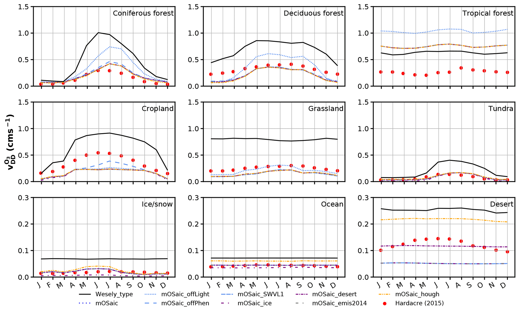
Figure 7Average seasonal cycles of ozone dry deposition velocities separated by land use type. Results from Hardacre et al. (2015) are shown as a reference. We refrain from showing the full extent of EMEP_offLight here, since it is an extreme scenario and has been discussed already.
Finally, we take a look at the different global as well as hemispheric dry deposition sinks for ozone (Table 3). Despite its vastness, the ocean amounts only to 35 % of the global ozone sink due to dry deposition in Oslo CTM3 with the operative mOSaic scheme (mOSaic), while permanently ice- and snow-covered regions account for 1.2 %. The remainder is deposited to land surfaces of which deserts might be the most neglected in process modeling. The total annual dry deposition in the mOSaic scheme is one-third below the multi-model-mean result by Hardacre et al. (2015). But also the results of Luhar et al. (2017, 2018) yield a 19 %–27 % lower ozone dry deposition than the models participating in the model intercomparison, with deposition to ocean ranging between 12 % and 21 % of the total annual ozone dry deposition. In particular, Luhar et al. (2018) found that current model estimates of ozone dry deposition to the ocean may be 3 times too high compared to their analysis. This implies that the ozone dry deposition to the ocean in Oslo CTM3 is too high as well.
Table 3Total ozone dry deposition for the respective model experiment in Tg a−1. The global ozone dry deposition has been weighted by ocean, ice, and land fraction in each grid box, respectively. “Ice” herein refers to regions at high latitudes that are permanently covered by ice and snow.
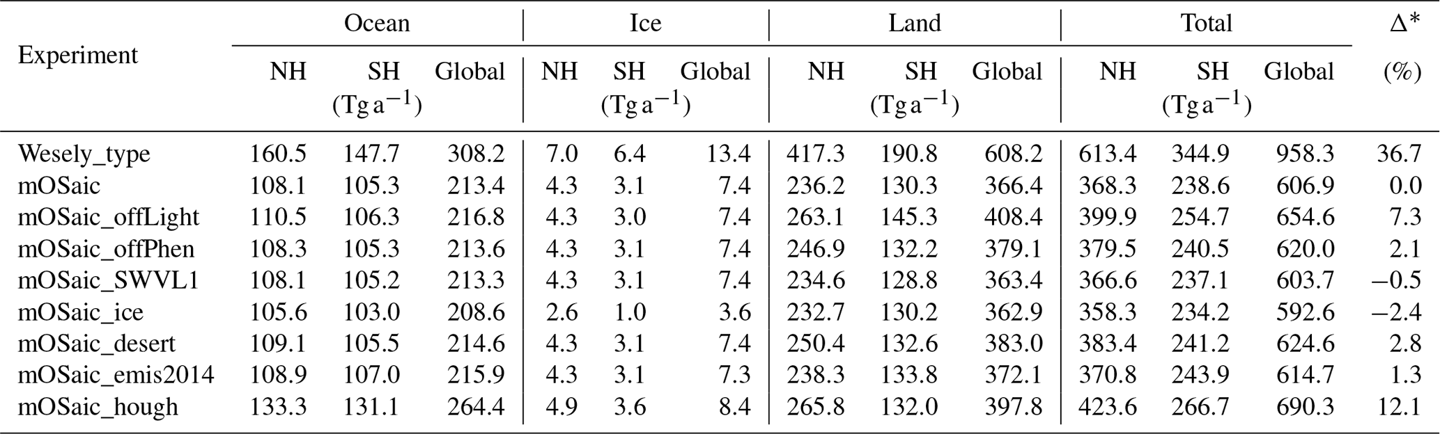
* Relative change of global annual total in comparison to mOSaic.
Table 4 displays the average tropospheric ozone burden for all model experiments. Consistent with the previous findings, the mOSaic scheme increases the tropospheric ozone burden by 35 Tg. From various satellite ozone retrieval products, Gaudel et al. (2018, Table 5) deduce a lower limit estimate for global tropospheric ozone burden for the years 2010–2014 of 333–345 Tg but remark that this amount underestimates the actual tropospheric ozone burden, since it is only based on daytime retrievals. Nevertheless, the results of mOSaic lie 17 % above that estimate and also well above the typical modeling range of 302–378 Tg (Young et al., 2013). Despite the strong positive bias in ozone concentrations and accordingly low bias in total dry deposition, the difference between mOSaic and mOSaic_emis2014 (6 Tg) lies well within the range given by satellites for the years 2005 and 2014 (Gaudel et al., 2018, Fig. 26). This indicates that Oslo CTM3 responds well to given changes in global emissions.
Table 4Annual mean tropospheric ozone burden for all experiments and 1σ standard deviation.

3.3 Comparison with MACC reanalysis
In this section, we conclude the comparison of our results with respect to global ozone by looking at ECMWF's MACC reanalysis (MACC-II Consortium, 2011, data obtained from ECWMF's data center; https://apps.ecmwf.int/datasets/data/macc-reanalysis/levtype=ml/, last access: 8 July 2019). In Fig. 8, we compare mOSaic ozone concentrations in the lowermost model level with surface concentrations deduced from the MACC reanalysis for the year 2005. The MACC reanalysis displays low ozone concentrations above all land masses except for the Greenland ice sheet. The lowest values are found in the deep tropics (e.g., northern South America and central Africa), while the highest values occur within 25–60∘ N over the oceans. These low values over the oceans are relatively well reproduced by mOSaic (±20 %). Over, e.g., South America, central and southern Africa, the Arabian Peninsula, and the northwestern Indian subcontinent, the ozone concentrations are elevated by up to 200 %. Regarding the global average surface ozone concentration, Wesely_type (Sect. S8) is more consistent with the MACC reanalysis than mOSaic but shows the same tendency of enhanced ozone over the continents as the latter. This enhancement is apparent mostly in the deep tropics and over the northwestern Indian subcontinent, which coincides with regions of high intensity in incoming UV radiation. This may indicate an imbalance in the photochemical production and loss of O3 in Oslo CTM3.

Figure 8Mean ozone concentrations for the year 2005. (a) MACC reanalysis (surface); (b) Oslo CTM3 mOSaic (lowermost model level); (c) relative difference.
3.4 Comparison with ground-based observations
In this section, we compare our model results to observations at a selected number of sites which provide ozone flux measurements. For all comparisons, we use the original resolution of Oslo CTM3 () instead of the regridded resolution ().
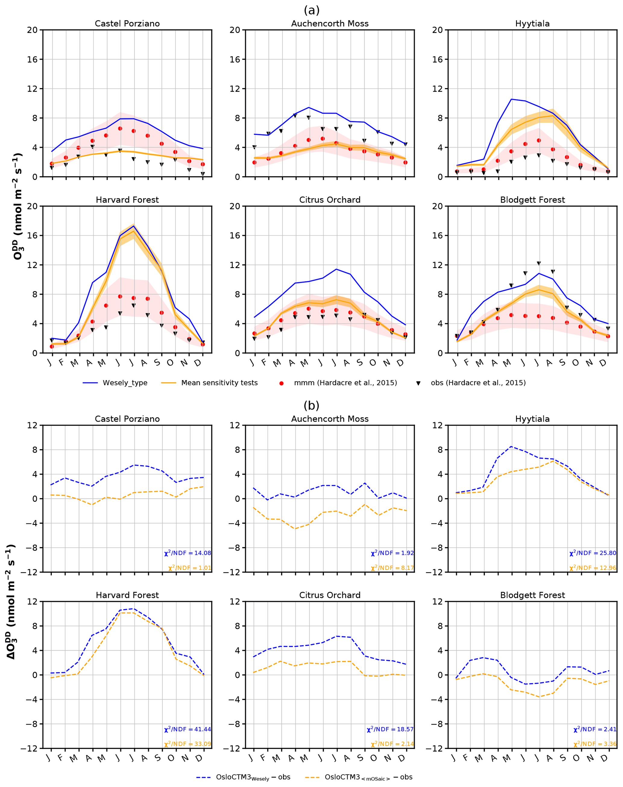
Figure 9Ozone dry deposition fluxes at different observation sites. (a) Comparison between Wesely scheme and average result from all sensitivity studies with observational averages taken from Hardacre et al. (2015). The model uncertainty of Oslo CTM3 is given as a 1 σ error band. The shaded area around the multi-model mean indicates the broad range of different model results but is not an actual error band. (b) Model divergence from observation and χ2-test results.
In Fig. 9a, seasonal cycles of average ozone dry deposition fluxes for the six selected observation sites are shown. We have computed a model average for all sensitivity studies at the closest grid point and show the 1 σ uncertainty band. The shaded area around the multi-model mean indicates the broad range of model results but is not an actual uncertainty band since such is not given in Hardacre et al. (2015). At four of the six sites, the mOSaic scheme performs better than the Wesely scheme and similar to or better than the multi-model mean. We use a χ2 test:
with an estimated standard deviation of observation σi=1 and divide it by the number of degrees of freedom (NDF) to assess this subjective analysis in a more objective way. The closer to 1 this test scores, the better the simulation represents the observation. A score between 0 and 1 indicates that the estimated σ is too small. The results of the χ2 test are shown together with the divergences in Fig. 9b. The χ2 test reveals also that in four of the six cases the mOSaic scheme improves the performance of Oslo CTM3 with respect to observed ozone dry deposition fluxes, although a satisfying result is only achieved for two sites (Castel Porziano, Blodgett Forest). With only one full year of simulation, the model uncertainty regarding the seasonal cycle at observational sites cannot be properly quantified. Furthermore, the observational averages comprise at most 9 years worth of data. Statistically, these data may still be subject to interannual variability. Among other aspects, the horizontal as well as vertical resolution play an important role in the model performance. Although we do not explicitly assess the impacts of differing resolutions in our model, we can assume that both high and low biases exist due to dilution of sources and sinks in coarse-resolution models (Schaap et al., 2015). Good matches between observation and model are only to be expected if the station's location is representative of an area similar to the respective model grid box and not substantially affected by differences in modeled and actual topography (e.g., major wind directions).
We have presented an update of the dry deposition scheme in Oslo CTM3 from purely prescribed dry deposition velocities (Wesely, 1989; Hough, 1991) to a more process-oriented parameterization taking the state of the atmosphere and vegetation into account. Based on the description of dry deposition in Simpson et al. (2003, 2012), we have implemented a mosaic approach to compute contributions to dry deposition by individual subgrid land surface types. Aerodynamic, quasi-laminar, and surface resistance (with the latter divided into stomatal and non-stomatal contributions) is calculated for each land surface category separately. Based on these, a land fraction-weighted mean is deduced. In addition, the various dry deposition velocities are now directly available from model output for diagnostics and further studies.
The new dry deposition scheme named mOSaic improves the modeled dry deposition velocities which are now compatible with observation and model studies (e.g., Hardacre et al., 2015; Luhar et al., 2018). Dry deposition velocities are reduced by 6 %–60 %. At the same time, the annual amount of ozone dry deposition decreases by more than 100 % over all major desert areas and increases over tropical forest. Compared to results from a multi-model evaluation (Hardacre et al., 2015), the total annual ozone dry deposition in Oslo CTM3 is % below average. However, there seems to be a tendency that newer TF HTAP models show a lower total annual dry deposition of ozone than older models, indicating that newer developments lead to decreasing ozone dry deposition and increasing tropospheric ozone burden (e.g., Luhar et al., 2017, 2018; Hu et al., 2017).
We found the response of Oslo CTM3 to the changes in dry deposition velocities from the old and the mOSaic scheme to be consistent. A decrease in leads to a decrease in total ozone dry deposition and an increase in ozone concentration [O3]. As the new scheme is quantitatively more similar to the multi-model mean (Hardacre et al., 2015) with respect to dry deposition velocities, while the old scheme agrees better in terms of total dry deposition, there is an apparent discrepancy. By means of tropospheric ozone burden (Gaudel et al., 2018) and surface ozone concentrations deduced from the MACC reanalysis (MACC-II Consortium, 2011), Oslo CTM3 with the operational mOSaic scheme shows a pronounced high bias of tropospheric ozone. While the average bias is small or even reversed when using the old scheme, both display elevated ozone in comparison with the MACC reanalysis in continental regions with high average incoming UV radiation (e.g., northern South America, central and southern Africa, the Himalayas). The reason behind this bias has not yet been resolved and may hint at, e.g., issues in photochemistry ([OH]-related ozone production and loss) or previously introduced optimization of ozone removal with respect to the old, less physical dry deposition velocities.
Most of the qualitative change in ozone dry deposition in Oslo CTM3 (−2 %–12 %) can be attributed to changes in dry deposition over the ocean and deserts. This is mainly due to updates of the respective prescribed ozone surface resistance . In the case of desert and grasslands, the difference between the old and new prescribed values is an order of magnitude. Over the ocean, the absolute change in dry deposition is small, but it is accumulated over a large area which is especially amplified in the Southern Hemisphere. Small adjustments to the lower limits in our quasi-laminar layer resistance formulation may help improve Oslo CTM3 performance in this regard. With respect to available measurements of dry deposition velocities of ozone over desert (Güsten et al., 1996) and ocean (Helmig et al., 2012), the new Oslo CTM3 dry deposition scheme slightly underestimates ozone dry deposition velocities over the former and overestimates them over the latter. Regarding the vastness of the ocean and the ongoing desertification, it may be worthwhile to revise the dry deposition scheme for these regimes and add more process-oriented formulations, e.g., two-layer gas exchange with ocean waters (Luhar et al., 2017, 2018), wave breaking and spray (Pozzer et al., 2006).
Although dry deposition to ice and snow amounts to only 1 % of the total global annual ozone dry deposition in mOSaic, a decrease in prescribed dry deposition velocity in accordance with combined measurements and model studies (Helmig et al., 2007) causes almost a doubling in the surface ozone concentrations in the high Arctic and affects surface ozone concentrations down to latitudes at 50∘ in both hemispheres. Comparing with results from the multi-model evaluation (Hardacre et al., 2015), we conclude that it is important to use this updated ozone dry deposition velocity to counter an Arctic surface ozone low bias in models; however, this currently leads to an overcompensation (high bias) in Oslo CTM3.
We have studied the parameter space of the stomatal conductance parameterization and found that surface ozone in the tropics and the Northern Hemisphere is most sensitive to changes therein. In the most extreme test case, the increase in global total dry deposition amounts to 7.3 %, while the more realistic test cases, e.g., using differing years of emission, amount to changes of the order of ±2 %. This may indicate that future changes in vegetation cover and solar radiation at the surface due to changes in stratospheric ozone, cloud cover, or aerosols could also strongly influence the surface ozone burden in the tropics. Total column ozone in the tropics is predicted to decrease due to changes in the atmospheric circulation (e.g., WMO – Global Ozone Research and Monitoring Project, 2014), while tropospheric and surface ozone increase. The combined effects of increasing emissions of ozone precursors and an increase in UV due to thinning of stratospheric ozone might permit more UV light at ground level and thus increase the ozone production.
An important factor in the global ozone budget is emissions of precursor substances. We cover this by using the same meteorology with different years of CEDS emissions. We chose the years 2005 and 2014 for our comparison. Ozone precursor emissions in 2014 are slightly lower in the NH while enhanced in the tropics and the SH. In 2014, surface ozone burden is higher in the Southern Hemisphere and in the tropics (5 %) compared to 2005, while it is lower in the Northern Hemisphere (2 %).
We also evaluated the model with respect to observed dry deposition fluxes at six sites in the Northern Hemisphere and found that the mOSaic scheme performs better than the old one but is not able to reproduce the measurements at most sites quantitatively. This may be due to several reasons. The model resolution in both horizontal () and vertical (L60, Pmax=0.02 hPa) does not capture all details in transport, thus affecting the distribution and transport (e.g., long-range, convection, and stratosphere–troposphere exchange) of ozone and its precursors. Depending on the location of the observation site and its respective representativeness for a larger area, ozone dry deposition and ozone concentrations are expected to be over- or underestimated in the model. Because of non-linearities in ozone formation and destruction, ozone concentrations are sensitive to both differences in local concentration of precursors and meteorological conditions (Jin et al., 2013). In addition, a comparison of very few years of measurement to only one specific year of simulation may reflect the year-to-year variability more than the actual model performance.
Future work on Oslo CTM3 should resolve the ozone high bias which may involve revising the photolysis and chemical reaction computation as well as reaction rates. For a better modeling of ozone abundances, ocean emissions of very-short-lived ozone-depleting substances (VSLSs) (Warwick et al., 2006; Ziska et al., 2013) which affect stratospheric ozone (Hossaini et al., 2016; Falk et al., 2017) and a scheme covering Arctic springtime ozone depletion (e.g., Yang et al., 2010; Toyota et al., 2011; Falk and Sinnhuber, 2018) could be worthwhile to implement. The general model performance could also be improved by allowing for more plant functional types and phenologies than currently used or implementing an actual photosynthesis-based modeling of plants. A more efficient parallelization of the code would enable computation at higher horizontal resolutions.
Oslo CTM3 shall be publicly available on GitHub under an MIT license in the future. Until then, access can be granted upon request. Model results can be made available upon request.
The used LAI and roughness length (z0) are available online from Oak Ridge National Laboratory Distributed Active Archive Center, Oak Ridge, Tennessee, USA (https://doi.org/10.3334/ORNLDAAC/970; Sietse et al., 2010).
CEDS historical emission inventory is provided by the Joint Global Research Institute project (http://www.globalchange.umd.edu/ceds/; Joint Global Change Research Institute, 2007).
Data from the Global Fire Emissions Database, Version 4, (GFEDv4) are available online from Oak Ridge National Laboratory Distributed Active Archive Center, Oak Ridge, Tennessee, USA (https://doi.org/10.3334/ORNLDAAC/1293; Randerson et al., 2018).
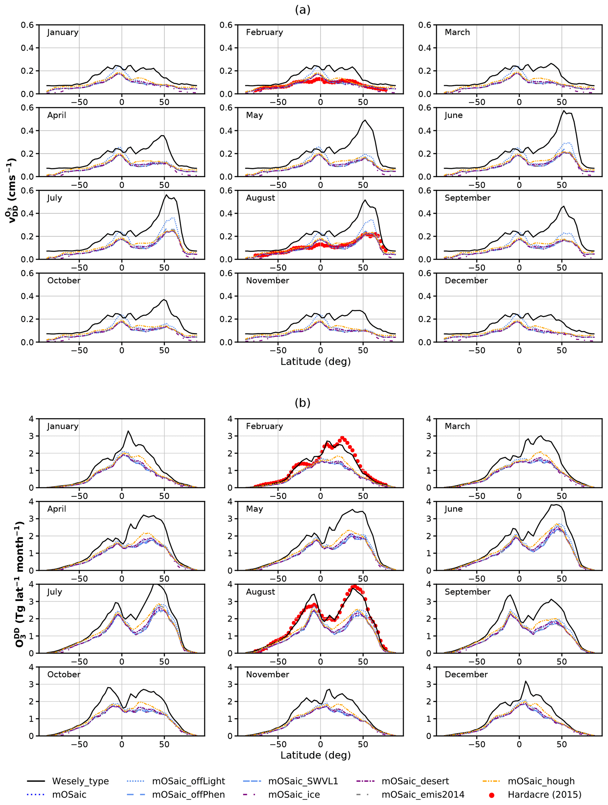
Figure A1Comparison of the manifold Oslo CTM3 integrations with respect to (a) zonal average ozone dry deposition velocities and (b) total annual amount of ozone removed from the atmosphere via dry deposition. The multi-model mean from the evaluation of TF HTAP models by Hardacre et al. (2015) is shown as a reference (where available).
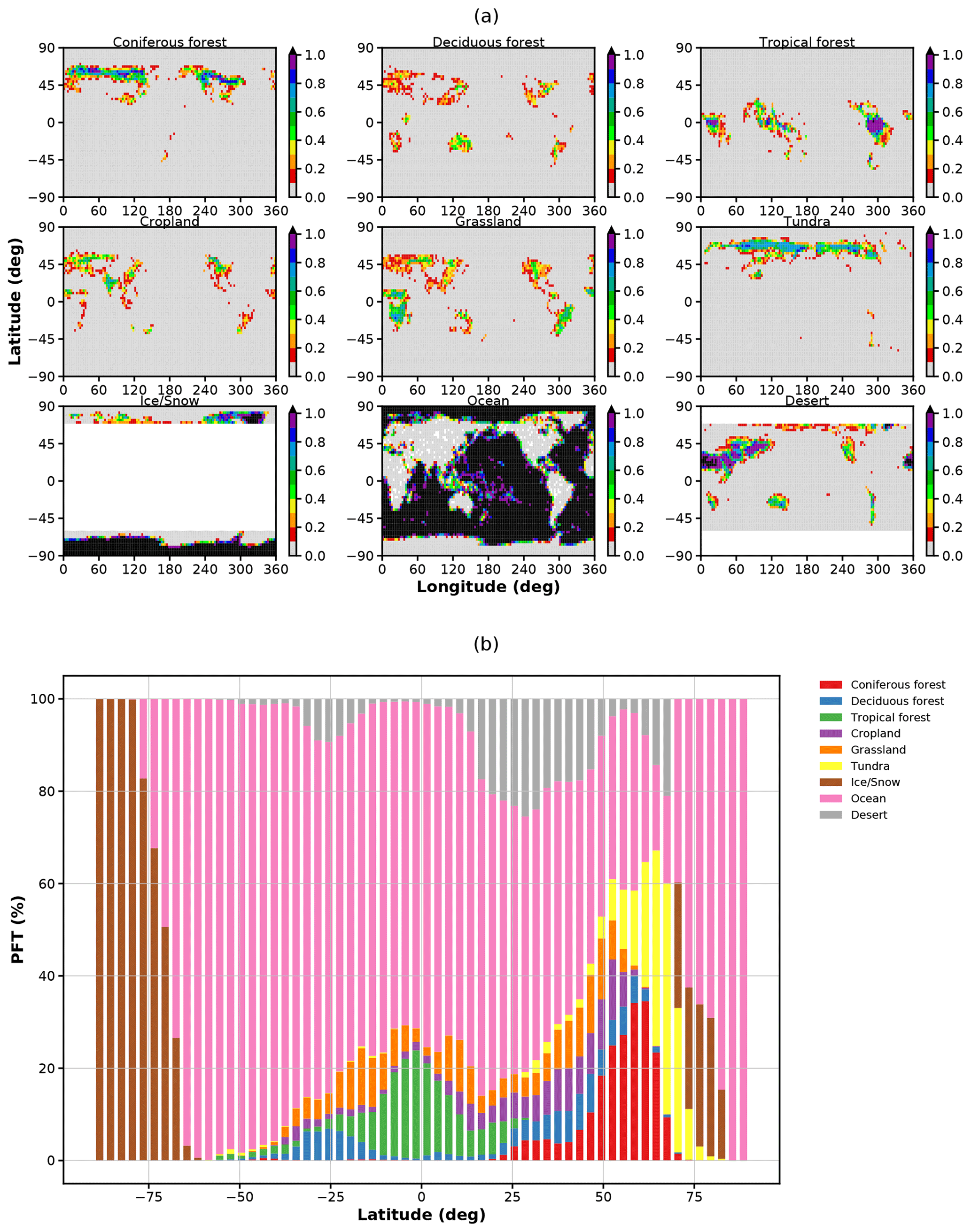
Figure A2Partitioning of land surface types: (a) CLM 2 dynamic land surface types in resolution; (b) zonal distribution of land surface types.
The supplement related to this article is available online at: https://doi.org/10.5194/gmd-12-4705-2019-supplement.
SF compiled the manuscript, finalized and revised the implementation of the stomatal conductance in the mOSaic dry deposition scheme of Oslo CTM3, conducted the simulations, and analyzed and evaluated the results. ASH implemented the mOSaic dry deposition scheme and wrote the respective documentation. Both authors contributed to the writing and discussion of the paper.
The authors declare that they have no conflict of interest.
This work was supported by the Norwegian Research Council (NRC) through the project “The double punch: Ozone and climate stresses on vegetation” (268073).
The simulations were performed on resources provided by UNINETT Sigma2 – the National Infrastructure for High Performance Computing and Data Storage in Norway (project nn2806k).
We would like to thank Frode Stordal (Section for Meteorology and Oceanography, University of Oslo) for discussions regarding early drafts of the manuscript, Anne Fouilloux (scientific programmer at the same institute) for technical support as well as Olimpia Bruno (Karlsruhe Institute of Technology), and Franziska Hellmuth (University of Oslo) for valuable input regarding the aerodynamic resistance formulation. We would also like to thank the Center for International Climate Research (CICERO) for their support of this work.
This research has been supported by the Norwegian Research Council (grant no. 268073).
This paper was edited by Fiona O'Connor and reviewed by David Simpson and one anonymous referee.
Ainsworth, E. A.: Understanding and improving global crop response to ozone pollution, Plant J., 90, 886–897, https://doi.org/10.1111/tpj.13298, 2017. a
Anav, A., Liu, Q., De Marco, A., Proietti, C., Savi, F., Paoletti, E., and Piao, S.: The role of plant phenology in stomatal ozone flux modeling, Glob. Change Biol., 24, 235–248, https://doi.org/10.1111/gcb.13823, 2017. a, b
Anderson, M. C., Norman, J. M., Meyers, T. P., and Diak, G. R.: An analytical model for estimating canopy transpiration and carbon assimilation fluxes based on canopy light-use efficiency, Agr. Forest Meteorol., 101, 265–289, https://doi.org/10.1016/S0168-1923(99)00170-7, 2000. a
Ball, J., Woodrow, I., and Berry, J.: A Model Predicting Stomatal Conductance and its Contribution to the Control of Photosynthesis under Different Environmental Conditions, in: Progress in Photosynthesis Research, edited by: Biggins, J., Springer, Dordrecht, 221–224, 1987. a, b
Buckley, T. N.: Modeling Stomatal Conductance, Plant Physiol., 174, 572–582, https://doi.org/10.1104/pp.16.01772, 2017. a
Charnock, H.: Wind stress on a water surface, Q. J. Roy. Meteor. Soc., 81, 639–640, https://doi.org/10.1002/qj.49708135027, 1955. a
Chuwah, C., van Noije, T., van Vuuren, D. P., Stehfest, E., and Hazeleger, W.: Global impacts of surface ozone changes on crop yields and land use, Atmos. Environ., 106, 11–23, https://doi.org/10.1016/j.atmosenv.2015.01.062, 2015. a
Derwent, R. G., Parrish, D. D., Galbally, I. E., Stevenson, D. S., Doherty, R. M., Naik, V., and Young, P. J.: Uncertainties in models of tropospheric ozone based on Monte Carlo analysis: Tropospheric ozone burdens, atmospheric lifetimes and surface distributions, Atmos. Environ., 180, 93–102, https://doi.org/10.1016/j.atmosenv.2018.02.047, 2018. a
Emberson, L. D., Simpson, D., Tuovinen, J.-P., Ashmore, M. R., and Cambridge, H. M.: Towards a model of ozone deposition and stomatal uptake over Europe, Det Norske Meteorologiske Institutt, Research Note No. 42, 2000. a
Erisman, J. W., Van Pul, A., and Wyers, P.: Parametrization of Surface-Resistance for the Quantification of Atmospheric Deposition of Acidifying Pollutants and Ozone, Atmos. Environ., 28, 2595–2607, https://doi.org/10.1016/1352-2310(94)90433-2, 1994. a
Falk, S. and Sinnhuber, B.-M.: Polar boundary layer bromine explosion and ozone depletion events in the chemistry–climate model EMAC v2.52: implementation and evaluation of AirSnow algorithm, Geosci. Model Dev., 11, 1115–1131, https://doi.org/10.5194/gmd-11-1115-2018, 2018. a
Falk, S., Sinnhuber, B.-M., Krysztofiak, G., Jöckel, P., Graf, P., and Lennartz, S. T.: Brominated VSLS and their influence on ozone under a changing climate, Atmos. Chem. Phys., 17, 11313–11329, https://doi.org/10.5194/acp-17-11313-2017, 2017. a
Fleming, Z. L., Doherty, R. M., von Schneidemesser, E., Malley, C. S., Cooper, O. R., Pinto, J. P., Colette, A., Xu, X., Simpson, D., Schultz, M. G., Lefohn, A. S., Hamad, S., Moolla, R., Solberg, S., and Feng, Z.: Tropospheric Ozone Assessment Report: Present-day ozone distribution and trends relevant to human health, Elementa, 6, 12, https://doi.org/10.1525/elementa.273, 2018. a
Fu, Y., Zhang, H., Dong, W., and Yuan, W.: Comparison of Phenology Models for Predicting the Onset of Growing Season over the Northern Hemisphere, Plos One, 9, e109544, https://doi.org/10.1371/journal.pone.0109544, 2014a. a
Fu, Y. H., Piao, S., Zhao, H., Jeong, S.-J., Wang, X., Vitasse, Y., Ciais, P., and Janssens, I. A.: Unexpected role of winter precipitation in determining heat requirement for spring vegetation green-up at northern middle and high latitudes, Glob. Change Biol., 20, 3743–3755, https://doi.org/10.1111/gcb.12610, 2014b. a
Garratt, J. R.: The Atmospheric Boundary Layer, University Press, Cambridge, 1992. a, b, c
Gaudel, A., Cooper, O. R., Ancellet, G., Barret, B., Boynard, A., Burrows, J. P., Clerbaux, C., Coheur, P. F., Cuesta, J., Cuevas, E., Doniki, S., Dufour, G., Ebojie, F., Foret, G., Garcia, O., Granados-Munoz, M. J., Hannigan, J. W., Hase, F., Hassler, B., Huang, G., Hurtmans, D., Jaffe, D., Jones, N., Kalabokas, P., Kerridge, B., Kulawik, S., Latter, B., Leblanc, T., Le Flochmoen, E., Lin, W., Liu, J., Liu, X., Mahieu, E., McClure-Begley, A., Neu, J. L., Osman, M., Palm, M., Petetin, H., Petropavlovskikh, I., Querel, R., Rahpoe, N., Rozanov, A., Schultz, M. G., Schwab, J., Siddans, R., Smale, D., Steinbacher, M., Tanimoto, H., Tarasick, D. W., Thouret, V., Thompson, A. M., Trickl, T., Weatherhead, E., Wespes, C., Worden, H. M., Vigouroux, C., Xu, X., Zeng, G., and Ziemke, J.: Tropospheric Ozone Assessment Report: Present-day distribution and trends of tropospheric ozone relevant to climate and global atmospheric chemistry model evaluation, Elementa, 6, 39, https://doi.org/10.1525/elementa.291, 2018. a, b, c
GEIA-ACCENT emission data portal: POET, online, Global CO emissions (1990–2000), available at: http://accent.aero.jussieu.fr/database_table_inventories.php (last access: 12 October 2017), 2003. a
Guenther, A., Karl, T., Harley, P., Wiedinmyer, C., Palmer, P. I., and Geron, C.: Estimates of global terrestrial isoprene emissions using MEGAN (Model of Emissions of Gases and Aerosols from Nature), Atmos. Chem. Phys., 6, 3181–3210, https://doi.org/10.5194/acp-6-3181-2006, 2006. a
Güsten, H., Heinrich, G., Mönnich, E., Sprung, D., Weppner, J., Ramadan, A. B., Ezz El-din, M. R. M., Ahmed, D. M., and Hassan, G. K. Y.: On-line measurements of ozone surface fluxes: Part II. Surface-level ozone fluxes onto the sahara desert, Atmos. Environ., 30, 911–918, https://doi.org/10.1016/1352-2310(95)00270-7, 1996. a, b, c, d
Hardacre, C., Wild, O., and Emberson, L.: An evaluation of ozone dry deposition in global scale chemistry climate models, Atmos. Chem. Phys., 15, 6419–6436, https://doi.org/10.5194/acp-15-6419-2015, 2015. a, b, c, d, e, f, g, h, i, j, k, l, m, n, o, p, q, r, s, t
Helmig, D., Ganzeveld, L., Butler, T., and Oltmans, S. J.: The role of ozone atmosphere-snow gas exchange on polar, boundary-layer tropospheric ozone – a review and sensitivity analysis, Atmos. Chem. Phys., 7, 15–30, https://doi.org/10.5194/acp-7-15-2007, 2007. a, b, c, d, e
Helmig, D., Lang, E. K., Bariteau, L., Boylan, P., Fairall, C. W., Ganzeveld, L., Hare, J. E., Hueber, J., and Pallandt, M.: Atmosphere-ocean ozone fluxes during the TexAQS 2006, STRATUS 2006, GOMECC 2007, GasEx 2008, and AMMA 2008 cruises, J. Geophys. Res.-Atmos., 117, D04305, https://doi.org/10.1029/2011JD015955, 2012. a, b
Hinze, J. O.: Turbulence, McGraw-Hill Series in Mechanical Engineering, McGraw-Hill, New York, p. 790, 1975. a
Hoesly, R. M., Smith, S. J., Feng, L., Klimont, Z., Janssens-Maenhout, G., Pitkanen, T., Seibert, J. J., Vu, L., Andres, R. J., Bolt, R. M., Bond, T. C., Dawidowski, L., Kholod, N., Kurokawa, J.-I., Li, M., Liu, L., Lu, Z., Moura, M. C. P., O'Rourke, P. R., and Zhang, Q.: Historical (1750–2014) anthropogenic emissions of reactive gases and aerosols from the Community Emissions Data System (CEDS), Geosci. Model Dev., 11, 369–408, https://doi.org/10.5194/gmd-11-369-2018, 2018. a, b
Hoshika, Y., Katata, G., Deushi, M., Watanabe, M., Koike, T., and Paoletti, E.: Ozone-induced stomatal sluggishness changes carbon and water balance of temperate deciduous forests, Sci. Rep.-UK, 5, 9871, https://doi.org/10.1038/srep09871, 2015. a
Hossaini, R., Patra, P. K., Leeson, A. A., Krysztofiak, G., Abraham, N. L., Andrews, S. J., Archibald, A. T., Aschmann, J., Atlas, E. L., Belikov, D. A., Bönisch, H., Carpenter, L. J., Dhomse, S., Dorf, M., Engel, A., Feng, W., Fuhlbrügge, S., Griffiths, P. T., Harris, N. R. P., Hommel, R., Keber, T., Krüger, K., Lennartz, S. T., Maksyutov, S., Mantle, H., Mills, G. P., Miller, B., Montzka, S. A., Moore, F., Navarro, M. A., Oram, D. E., Pfeilsticker, K., Pyle, J. A., Quack, B., Robinson, A. D., Saikawa, E., Saiz-Lopez, A., Sala, S., Sinnhuber, B.-M., Taguchi, S., Tegtmeier, S., Lidster, R. T., Wilson, C., and Ziska, F.: A multi-model intercomparison of halogenated very short-lived substances (TransCom-VSLS): linking oceanic emissions and tropospheric transport for a reconciled estimate of the stratospheric source gas injection of bromine, Atmos. Chem. Phys., 16, 9163–9187, https://doi.org/10.5194/acp-16-9163-2016, 2016. a
Hough, A. M.: Development of a 2-Dimensional Global Tropospheric Model – Model Chemistry, J. Geophys. Res.-Atmos., 96, 7325–7362, https://doi.org/10.1029/90JD01327, 1991. a, b, c, d, e, f
Hu, L., Jacob, D. J., Liu, X., Zhang, Y., Zhang, L., Kim, P. S., Sulprizio, M. P., and Yantosca, R. M.: Global budget of tropospheric ozone: Evaluating recent model advances with satellite (OMI), aircraft (IAGOS), and ozonesonde observations, Atmos. Environ., 167, 323–334, https://doi.org/10.1016/j.atmosenv.2017.08.036, 2017. a
IPCC – Intergovernmental Panel on Climate Change: Climate Change 2013: The Physical Science Basis, 2013. a, b, c, d, e
Jarvis, P. G.: The interpretation of the variations in leaf water potential and stomatal conductance found in canopies in the field, Philos. T. Roy. Soc. B., 273, 593–610, https://doi.org/10.1098/rstb.1976.0035, 1976. a
Jin, L., Loisy, A., and Brown, N.: Role of meteorological processes in ozone responses to emission controls in California's San Joaquin Valley, J. Geophys. Res.-Atmos., 118, 8010–8022, https://doi.org/10.1002/jgrd.50559, 2013. a, b
Joint Global Change Research Institute: A Community Emissions Data System (CEDS) for Historical Emissions, available at: http://www.globalchange.umd.edu/ceds/, last access: 1 August 2017. a
Levis, S. and Bonan, G. B.: Simulating springtime temperature patterns in the community atmosphere model coupled to the community land model using prognostic leaf area, J. Climate, 17, 4531–4540, https://doi.org/10.1175/3218.1, 2004. a
Luhar, A. K., Galbally, I. E., Woodhouse, M. T., and Thatcher, M.: An improved parameterisation of ozone dry deposition to the ocean and its impact in a global climate–chemistry model, Atmos. Chem. Phys., 17, 3749–3767, https://doi.org/10.5194/acp-17-3749-2017, 2017. a, b, c, d, e, f
Luhar, A. K., Woodhouse, M. T., and Galbally, I. E.: A revised global ozone dry deposition estimate based on a new two-layer parameterisation for air–sea exchange and the multi-year MACC composition reanalysis, Atmos. Chem. Phys., 18, 4329–4348, https://doi.org/10.5194/acp-18-4329-2018, 2018. a, b, c, d, e, f, g, h
Lund, M. T., Myhre, G., Haslerud, A. S., Skeie, R. B., Griesfeller, J., Platt, S. M., Kumar, R., Myhre, C. L., and Schulz, M.: Concentrations and radiative forcing of anthropogenic aerosols from 1750 to 2014 simulated with the Oslo CTM3 and CEDS emission inventory, Geosci. Model Dev., 11, 4909–4931, https://doi.org/10.5194/gmd-11-4909-2018, 2018. a
MACC-II Consortium: MACC Reanalysis of Global Atmospheric Composition (2003–2012), Copernicus Atmosphere Monitoring Service (CAMS) available at: https://atmosphere.copernicus.eu/catalogue#/ (last access: 8 July 2019), 2011. a, b, c
Matyssek, R., Wieser, G., Calfapietra, C., de Vries, W., Dizengremel, P., Ernst, D., Jolivet, Y., Mikkelsen, T. N., Mohren, G. M. J., Le Thiec, D., Tuovinen, J. P., Weatherall, A., and Paoletti, E.: Forests under climate change and air pollution: Gaps in understanding and future directions for research, Environ. Pollut., 160, 57–65, https://doi.org/10.1016/j.envpol.2011.07.007, 2012. a
Mills, G., Sharps, K., Simpson, D., Pleijel, H., Broberg, M., Uddling, J., Jaramillo, F., Davies, W. J., Dentener, F., Van den Berg, M., Agrawal, M., Agrawal, S. B., Ainsworth, E. A., Büker, P., Emberson, L., Feng, Z., Harmens, H., Hayes, F., Kobayashi, K., Paoletti, E., and Van Dingenen, R.: Ozone pollution will compromise efforts to increase global wheat production, Glob. Change Biol., 24, 3560–3574, https://doi.org/10.1111/gcb.14157, 2018. a
Mills, G., Harmens, H., Hayes, F., Pleijel, H., Büker, P., González-Fernandéz, I., Alonso, R., Bender, J., Bergmann, E. Bermejo, V., Braun, S., Danielsson, H., Gerosa, G., Grünhage, L., Karlsson, P. E., Marzuoli, R., Schaub, M., and Simpson, D.: Mapping Critical Levels for Vegetation, chap. III, in: ICP Mapping Manual, International Cooperative Programme on Effects of Air Pollution on Natural Vegetation and Crops, available at: https://icpmapping.org/Latest_update_Mapping_Manual (last access: 11 February 2019), 2017. a, b
Mills, G., Pleijel, H., Malley, C. S., Sinha, B., Cooper, O. R., Schultz, M. G., Neufeld, H. S., Simpson, D., Sharps, K., Feng, Z., Gerosa, G., Harmens, H., Kobayashi, K., Saxena, P., Paoletti, E., Sinha, V., and Xu, X.: Tropospheric Ozone Assessment Report: Present-day tropospheric ozone distribution and trends relevant to vegetation, Elementa, 6, 47, https://doi.org/10.1525/elementa.302, 2018. a
Monks, P. S., Archibald, A. T., Colette, A., Cooper, O., Coyle, M., Derwent, R., Fowler, D., Granier, C., Law, K. S., Mills, G. E., Stevenson, D. S., Tarasova, O., Thouret, V., von Schneidemesser, E., Sommariva, R., Wild, O., and Williams, M. L.: Tropospheric ozone and its precursors from the urban to the global scale from air quality to short-lived climate forcer, Atmos. Chem. Phys., 15, 8889–8973, https://doi.org/10.5194/acp-15-8889-2015, 2015. a, b, c, d
Otero, N., Sillmann, J., Mar, K. A., Rust, H. W., Solberg, S., Andersson, C., Engardt, M., Bergström, R., Bessagnet, B., Colette, A., Couvidat, F., Cuvelier, C., Tsyro, S., Fagerli, H., Schaap, M., Manders, A., Mircea, M., Briganti, G., Cappelletti, A., Adani, M., D'Isidoro, M., Pay, M.-T., Theobald, M., Vivanco, M. G., Wind, P., Ojha, N., Raffort, V., and Butler, T.: A multi-model comparison of meteorological drivers of surface ozone over Europe, Atmos. Chem. Phys., 18, 12269–12288, https://doi.org/10.5194/acp-18-12269-2018, 2018. a
Pozzer, A., Jöckel, P., Sander, R., Williams, J., Ganzeveld, L., and Lelieveld, J.: Technical Note: The MESSy-submodel AIRSEA calculating the air-sea exchange of chemical species, Atmos. Chem. Phys., 6, 5435–5444, https://doi.org/10.5194/acp-6-5435-2006, 2006. a
Randerson, J. T., van der Werf, G. R., Giglio, L., Collatz, G. J., and Kasibhatla, P. S.: Global Fire Emissions Database, Version 4, (GFEDv4), ORNL DAAC, Oak Ridge, Tennessee, USA, https://doi.org/10.3334/ORNLDAAC/1293, 2018. a, b
Schaap, M., Cuvelier, C., Hendriks, C., Bessagnet, B., Baldasano, J. M., Colette, A., Thunis, P., Karam, D., Fagerli, H., Graff, A., Kranenburg, R., Nyiri, A., Pay, M. T., Rouil, L., Schulz, M., Simpson, D., Stern, R., Terrenoire, E., and Wind, P.: Performance of European chemistry transport models as function of horizontal resolution, Atmos. Environ., 112, 90–105, https://doi.org/10.1016/j.atmosenv.2015.04.003, 2015. a
Schnell, J. L., Prather, M. J., Josse, B., Naik, V., Horowitz, L. W., Cameron-Smith, P., Bergmann, D., Zeng, G., Plummer, D. A., Sudo, K., Nagashima, T., Shindell, D. T., Faluvegi, G., and Strode, S. A.: Use of North American and European air quality networks to evaluate global chemistry–climate modeling of surface ozone, Atmos. Chem. Phys., 15, 10581–10596, https://doi.org/10.5194/acp-15-10581-2015, 2015. a, b
Seinfeld, J. H. and Pandis, S. N.: Atmospheric Chemistry and Physics: From Air Pollution to Climate Change, chap. 19, John Wiley & Sons, New York, 2nd edn., 2006. a, b
Sietse, O. L., Hall, F. G., Collatz, G. J., Meeson, B. W., Los, S. O., Brown De Colstoun, E., and Landis, D. R.: ISLSCP II FASIR-adjusted NDVI Biophysical Parameter Fields, 1982-1998. ORNL DAAC, Oak Ridge, Tennessee, USA, https://doi.org/10.3334/ORNLDAAC/970, 2010. a
Simpson, D., Tuovinen, J. P., Emberson, L., and Ashmore, M. R.: Characteristics of an ozone deposition module II: Sensitivity analysis, Water Air Soil Poll., 143, 123–137, https://doi.org/10.1023/A:1022890603066, 2003. a, b, c, d, e
Simpson, D., Benedictow, A., Berge, H., Bergström, R., Emberson, L. D., Fagerli, H., Flechard, C. R., Hayman, G. D., Gauss, M., Jonson, J. E., Jenkin, M. E., Nyíri, A., Richter, C., Semeena, V. S., Tsyro, S., Tuovinen, J.-P., Valdebenito, Á., and Wind, P.: The EMEP MSC-W chemical transport model – technical description, Atmos. Chem. Phys., 12, 7825–7865, https://doi.org/10.5194/acp-12-7825-2012, 2012. a, b, c, d, e, f, g, h, i, j, k, l, m, n, o, p, q, r, s, t, u, v, w, x, y
Sindelarova, K., Granier, C., Bouarar, I., Guenther, A., Tilmes, S., Stavrakou, T., Müller, J.-F., Kuhn, U., Stefani, P., and Knorr, W.: Global data set of biogenic VOC emissions calculated by the MEGAN model over the last 30 years, Atmos. Chem. Phys., 14, 9317–9341, https://doi.org/10.5194/acp-14-9317-2014, 2014. a
Sitch, S., Cox, P. M., Collins, W. J., and Huntingford, C.: Indirect radiative forcing of climate change through ozone effects on the land-carbon sink, Nature, 448, 791–U4, https://doi.org/10.1038/nature06059, 2007. a
Søvde, O. A., Prather, M. J., Isaksen, I. S. A., Berntsen, T. K., Stordal, F., Zhu, X., Holmes, C. D., and Hsu, J.: The chemical transport model Oslo CTM3, Geosci. Model Dev., 5, 1441–1469, https://doi.org/10.5194/gmd-5-1441-2012, 2012. a
Stevenson, D. S., Dentener, F. J., Schultz, M. G., Ellingsen, K., van Noije, T. P. C., Wild, O., Zeng, G., Amann, M., Atherton, C. S., Bell, N., Bergmann, D. J., Bey, I., Butler, T., Cofala, J., Collins, W. J., Derwent, R. G., Doherty, R. M., Drevet, J., Eskes, H. J., Fiore, A. M., Gauss, M., Hauglustaine, D. A., Horowitz, L. W., Isaksen, I. S. A., Krol, M. C., Lamarque, J.-F., Lawrence, M. G., Montanaro, V., Müller, J.-F., Pitari, G., Prather, M. J., Pyle, J. A., Rast, S., Rodriguez, J. M., Sanderson, M. G., Savage, N. H., Shindell, D. T., Strahan, S. E., Sudo, K., and Szopa, S.: Multimodel ensemble simulations of present-day and near-future tropospheric ozone, J. Geophys. Res.-Atmos., 111, D08301, https://doi.org/10.1029/2005JD006338, 2005. a
Tai, A. P. K., Martin, M. V., and Heald, C. L.: Threat to future global food security from climate change and ozone air pollution, Nat. Clim. Change, 4, 817–821, https://doi.org/10.1038/NCLIMATE2317, 2014. a
Tang, H., Takigawa, M., Liu, G., Zhu, J., and Kobayashi, K.: A projection of ozone-induced wheat production loss in China and India for the years 2000 and 2020 with exposure-based and flux-based approaches, Glob. Change Biol., 19, 2739–2752, https://doi.org/10.1111/gcb.12252, 2013. a
Toyota, K., McConnell, J. C., Lupu, A., Neary, L., McLinden, C. A., Richter, A., Kwok, R., Semeniuk, K., Kaminski, J. W., Gong, S.-L., Jarosz, J., Chipperfield, M. P., and Sioris, C. E.: Analysis of reactive bromine production and ozone depletion in the Arctic boundary layer using 3-D simulations with GEM-AQ: inference from synoptic-scale patterns, Atmos. Chem. Phys., 11, 3949–3979, https://doi.org/10.5194/acp-11-3949-2011, 2011. a
Tuovinen, J. P., Ashmore, M. R., Emberson, L. D., and Simpson, D.: Testing and improving the EMEP ozone deposition module, Atmos. Environ., 38, 2373–2385, https://doi.org/10.1016/j.atmosenv.2004.01.026, 2004. a
Warwick, N. J., Pyle, J. A., Carver, G. D., Yang, X., Savage, N. H., O'Connor, F. M., and Cox, R. A.: Global modeling of biogenic bromocarbons, J. Geophys. Res.-Atmos., 111, D24305, https://doi.org/10.1029/2006JD007264, 2006. a
Wesely, M. L.: Parameterization Of Surface Resistances To Gaseous Dry Deposition In Regional-Scale Numerical-Models, Atmos. Environ., 23, 1293–1304, https://doi.org/10.1016/0004-6981(89)90153-4, 1989. a, b, c, d, e, f, g, h
WHO – World Health Organization: Health risks of ozone from long-range transboundary air pollution, 2008. a
Wittig, V. E., Ainsworth, E. A., Naidu, S. L., Karnosky, D. F., and Long, S. P.: Quantifying the impact of current and future tropospheric ozone on tree biomass, growth, physiology and biochemistry: a quantitative meta-analysis, Glob. Change Biol., 15, 396–424, https://doi.org/10.1111/j.1365-2486.2008.01774.x, 2009. a
WMO – Global Ozone Research and Monitoring Project: Scientific Assessment ofOzone Depletion, available at: https://www.wmo.int/pages/prog/arep/gaw/ozone_2014/full_report_TOC.html (last access: 29 October 2019), 2014. a, b
Wu, J.: Wind-Stress Coefficients Over Sea-Surface Near Neutral Conditions – A Revisit, J. Phys. Oceanogr., 10, 727–740, https://doi.org/10.1175/1520-0485(1980)010<0727:WSCOSS>2.0.CO;2, 1980. a
Yang, X., Pyle, J. A., Cox, R. A., Theys, N., and Van Roozendael, M.: Snow-sourced bromine and its implications for polar tropospheric ozone, Atmos. Chem. Phys., 10, 7763–7773, https://doi.org/10.5194/acp-10-7763-2010, 2010. a
Young, P. J., Archibald, A. T., Bowman, K. W., Lamarque, J.-F., Naik, V., Stevenson, D. S., Tilmes, S., Voulgarakis, A., Wild, O., Bergmann, D., Cameron-Smith, P., Cionni, I., Collins, W. J., Dalsøren, S. B., Doherty, R. M., Eyring, V., Faluvegi, G., Horowitz, L. W., Josse, B., Lee, Y. H., MacKenzie, I. A., Nagashima, T., Plummer, D. A., Righi, M., Rumbold, S. T., Skeie, R. B., Shindell, D. T., Strode, S. A., Sudo, K., Szopa, S., and Zeng, G.: Pre-industrial to end 21st century projections of tropospheric ozone from the Atmospheric Chemistry and Climate Model Intercomparison Project (ACCMIP), Atmos. Chem. Phys., 13, 2063–2090, https://doi.org/10.5194/acp-13-2063-2013, 2013. a, b
Ziska, F., Quack, B., Abrahamsson, K., Archer, S. D., Atlas, E., Bell, T., Butler, J. H., Carpenter, L. J., Jones, C. E., Harris, N. R. P., Hepach, H., Heumann, K. G., Hughes, C., Kuss, J., Krüger, K., Liss, P., Moore, R. M., Orlikowska, A., Raimund, S., Reeves, C. E., Reifenhäuser, W., Robinson, A. D., Schall, C., Tanhua, T., Tegtmeier, S., Turner, S., Wang, L., Wallace, D., Williams, J., Yamamoto, H., Yvon-Lewis, S., and Yokouchi, Y.: Global sea-to-air flux climatology for bromoform, dibromomethane and methyl iodide, Atmos. Chem. Phys., 13, 8915–8934, https://doi.org/10.5194/acp-13-8915-2013, 2013. a