Evaluation of leaf-level optical properties employed in land surface models

Vegetation optical properties have a direct impact on canopy absorption and scattering and are thus needed for modeling surface fluxes. Although plant functional type (PFT) classification varies between different land surface models (LSMs), their optical properties must be specified. The aim of this study is to revisit the “time-invariant optical properties table” of the Simple Biosphere (SiB) model (later referred to as the “SiB table”) presented 30 years ago by Dorman and Sellers (1989), which has since been adopted by many LSMs. This revisit was needed as many of the data underlying the SiB table were not formally reviewed or published or were based on older papers or on personal communications (i.e., the validity of the optical property source data cannot be inspected due to missing data sources, outdated citation practices, and varied estimation methods). As many of today's LSMs (e.g., the Community Land Model (CLM), the Jena Scheme of Atmosphere Biosphere Coupling in Hamburg (JSBACH), and the Joint UK Land Environment Simulator (JULES)) either rely on the optical properties of the SiB table or lack references altogether for those they do employ, there is a clear need to assess (and confirm or correct) the appropriateness of those being used in today's LSMs. Here, we use various spectral databases to synthesize and harmonize the key optical property information of PFT classification shared by many leading LSMs. For forests, such classifications typically differentiate PFTs by broad geo-climatic zones (i.e., tropical, boreal, temperate) and phenology (i.e., deciduous vs. evergreen). For short-statured vegetation, such classifications typically differentiate between crops, grasses, and photosynthetic pathway. Using the PFT classification of the CLM (version 5) as an example, we found the optical properties of the visible band (VIS; 400–700 nm) to fall within the range of measured values. However, in the near-infrared and shortwave infrared bands (NIR and SWIR; e.g., 701–2500 nm, referred to as “NIR”) notable differences between CLM default and measured values were observed, thus suggesting that NIR optical properties are in need of an update. For example, for conifer PFTs, the measured mean needle single scattering albedo (SSA, i.e., the sum of reflectance and transmittance) estimates in NIR were 62 % and 78 % larger than the CLM default parameters, and for PFTs with flat leaves, the measured mean leaf SSA values in NIR were 20 %, 14 %, and 19 % larger than the CLM defaults. We also found that while the CLM5 PFT-dependent leaf angle values were sufficient for forested PFTs and grasses, for crop PFTs the default parameterization appeared too vertically oriented, thus warranting an update. In addition, we propose using separate bark reflectance values for conifer and deciduous PFTs and demonstrate how shoot-level clumping correction can be incorporated into LSMs to mitigate violations of turbid media assumption and Beer's law caused by the nonrandomness of finite-sized foliage elements.

1 Introduction

Vegetation optical properties have a direct impact on canopy absorption and scattering and are thus needed for modeling surface fluxes. All land surface models (LSMs) have modules to simulate radiation transfer (later referred to as “RT”) of surfaces. Although there are many types of canopy RT models with varying complexities – from light extinction algorithms to those applying turbid medium and geometric–optical methods – they must specify the following: optical properties (i.e., reflectance “R” and transmittance “T”) of canopy elements such as foliage and bark, canopy foliage area (e.g., leaf area index (LAI, m² m⁻²)), and vegetation spatial ordering (e.g., leaf inclination angle, LIA, i.e., the angle between the leaf surface normal and the zenith). At present, most LSMs are limited to one-dimensional (1-D) radiative exchange relying on solutions derived from two-stream approximations based on plane-parallel turbid media assumptions (Loew et al., 2014; Yuan et al., 2017).

Thirty years ago, Dorman and Sellers (1989) presented a “time-invariant optical properties table” for the Simple Biosphere (SiB) model (later referred to as the “SiB table” or “SiB classes”) which was compiled using available data and field notes of the time. To the best of our knowledge, some of these data, however, were either never subjected to formal peer-review and published (e.g., Miller, 1972; Klink and Willmot, 1985) or were based on earlier research citing even older papers or personal communications (i.e., the validity of the source data cannot be examined due to a lack of transparency). As many of today's LSMs (e.g., the Community Land Model (CLM) (Bonan et al., 2002), the land surface model developed at the Institut d'Astronomie et de Géophysique Georges Lemaître (IAGL) (de Ridder, 1997), the Jena Scheme of Atmosphere Biosphere Coupling in Hamburg (JSBACH, 2019), and the Joint UK Land Environment Simulator (JULES) (Clark et al., 2011)) either rely on the original SiB table optical properties or on undocumented data, there is a clear need to assess (and confirm or correct) the appropriateness of plant functional type (PFT)-dependent optical properties by benchmarking them to data collected and stored using present-day research norms and documentation standards.

Measurements of R and T spectra (λ) of leaves and needles can be achieved using integrating spheres (e.g., Hovi et al., 2017; Lukeš et al., 2013); R_(λ) of bark and short vegetation (i.e., grasses and crops) can be measured using handheld spectrometers (e.g., Lang et al., 2002) and LIA using inclinometers or digital photography (e.g., Ryu et al., 2010). Measured R_(λ) and T_(λ) can be averaged over different wavelength bands (e.g., visible (VIS), 400–700 nm; near-infrared and shortwave infrared (NIR and SWIR, later referred to as “NIR”), 701–2500 nm) required by LSMs, or resampled to correspond with different satellite sensors' band definitions (Asner et al., 1998). Although laboratory measurements of leaf optical properties have been done since the 1960s (Gates et al., 1965), compiling the spectra into public databases with other measured traits and metadata started relatively recently. Today's spectral libraries, such as EcoSIS (EcoSIS, 2017) and SPECCHIO (Hueni et al., 2009), are open databases for storing spectral data from different field campaigns to promote data usage by researchers and model developers. Some reputable example datasets stored in EcoSIS are “Lopex93” (Hosgood et al., 1993) and “Angers” (Jacquemound et al., 2003): Lopex93 and Angers contain data for species with flat leaves. For needleleaf species, spectral data are available from SPECCHIO. Reflectance spectra of different types of (hemi-)boreal grass species communities and tree bark are available, e.g., from the Estonian research database by Lang et al. (2002). Although many spectral data exist and are freely available, the earlier spectral datasets suffer from not being available online (e.g., data for 26 species from herbs to trees measured in Mississippi and Kansas, USA; Knapp and Carter, 1998) or having a limited wavelength range (e.g., BOREAS, comprising North American tree species, was limited to the wavelength range of 400–1100 nm; Middleton et al., 1997).

Similar to the developments of spectral databases, a wealth of information surrounding forest foliage LIA (^∘) has become available in recent years owing to new measurement techniques (e.g., Ryu et al., 2010). LIA is needed to obtain the direct beam extinction coefficient and, for example, to separate foliage area into sunlit and shaded parts as foliage responses to diffuse and direct solar radiation differ (Gu et al., 2002) and is also needed for RT model inversion (Combal et al., 2003). While measuring the LIA of grasses and crops is relatively straightforward and has been conducted since 1960 using inclined point quadrats by measuring the number of vegetation contacts from which the LIA is estimated (Warren Wilson, 1960), methods for measuring tree foliage LIA have been lacking due to problems applying them to tall forest canopies (i.e., the high cost of measurements and the inability to reproduce them). At present, a state-of-the-art method for determining LIAs is based on digital photography, which allows robust, nondestructive measurements (i.e., reproducible data) with low cost. In the absence of measured data, estimates regarding leaf angle distributions have often been obtained using modeling or have been assumed to be spherical (e.g., Oker-Blom and Kellomäki, 1982; Goudriaan, 1988). Based on a compilation of measured and published data, we assess the appropriateness of the PFT-dependent LIA parameterization used by today's LSMs.

In recent years, LSMs have been adapted to incorporate new important processes such as nutrient cycling and land cover dynamics, while the developments in biogeophysical processes like surface radiation schemes have not developed much further (Loew et al., 2014). Criticisms have dealt with incompatibilities in vegetation structural descriptions in the employed RT schemes (e.g., the MODIS LAI is based on three-dimensional (3-D) RT model, whereas the CLM employs a 1-D RT model) (Loew et al., 2014), which may lead to erroneous assessments of the absorbed, transmitted, and reflected fluxes (Pinty et al., 2004, 2006). This incompatibility can be avoided using effective state variables (i.e., effective LAI and effective optical properties), which translate the 3-D vegetation information into 1-D properties and correctly represent the effects of vegetation structural heterogeneity within a grid cell (e.g., Pinty et al., 2004; Wang et al., 2018). Effective state variables can be obtained by applying corrections that take into account vegetation nonrandomness (e.g., structure) or by measuring the clumped targets (e.g., conifer forest canopy; Majasalmi et al., 2017). The problem associated with clumping is caused by the turbid media assumption and Beer's law, which assume foliage elements to be infinitely small and randomly located, neither of which is true for non-gases. While clumping effects may appear at many scales (e.g., shoot, crown, tree, landscape) and may be corrected using various techniques (e.g., Norman and Jarvis, 1975; Chen and Black, 1992; Stenberg, 1996; Smolander and Stenberg, 2003; Haverd et al., 2012; He et al., 2012; Wang et al., 2018), there is consensus regarding the existence and significance of clumping in influencing the RT of a vegetation medium. It is noteworthy that currently clumping effects are not accounted for in LSMs.

The MODIS LAI algorithm (Knyazikhin et al., 1999), which is used to parameterize many LSMs, is based on a stochastic radiative transfer equation and a theory of spectral invariants, which packs 3-D information into a 1-D equation. This is possible as interactions between photons and canopy elements converge to invariant patterns, which can be quantified using a few wavelength-independent parameters, which satisfy the law of energy conservation (Wang et al., 2018). The MODIS LAI algorithm for needle forests (Sect. 2.2.6, Biome 6, in Knyazikhin et al., 1999) assumes needles to be clustered into shoots, with shoots being further clustered into crowns. Both clumping corrections are based on spectral invariants theory, which can be interpreted as “photon recollision probability” (p) (Smolander and Stenberg, 2005). The interpretation of p provides physical intuition with the mathematical concept and the association with measurable structural vegetation properties (e.g., Lewis and Disney, 2007; Rautiainen and Stenberg, 2005; Smolander and Stenberg, 2005). The p is a probability by which a photon scattered (reflected or transmitted) from a leaf or needle in the canopy will interact within the canopy again. In a canopy composed of leaves, a photon scattered from a leaf will not re-interact with the same leaf; however, in a canopy composed of shoots, a photon scattered out from a shoot may have interacted with the needles forming the shoot multiple times. The violations of turbid media assumption and Beer's law by needles clustering into shoots can be mitigated by changing the basic unit from a needle to a shoot (Nilson and Ross, 1997), by upscaling needle single scattering albedo spectra (SSA_needle(λ)) into shoot single scattering albedo spectra (SSA_shoot(λ)) based on shoot geometry (Rautiainen et al., 2012), and by simply replacing SSA_needle with effective SSA_shoot in the RT calculation. This correction is applicable to models employing turbid media assumption and Beer's law and provides the simplicity required by LSMs. In addition to the MODIS LAI algorithm, the p is currently incorporated into different types of RT modeling schemes such as the PARAS models (Stenberg et al., 2016) and the Forest Reflectance and Transmittance (FRT) model (Kuusk and Nilson, 2000).

There is large variation in the way optical properties can be defined (e.g., species composition) and measured (e.g., the measuring device and its wavelength range). Therefore, the main objective of this study is not to provide the “final truth” regarding PFT optical properties; rather, our aim is to assess their appropriateness by benchmarking them to data collected and stored using present-day research norms, reviewed and synthesized here. Specifically, our objectives are to (1) verify the PFT-dependent optical properties used in today's LSMs using the CLM PFT classification and optical property look-up table as an example; (2) suggest an alternative to account for shoot-level clumping of conifers in models employing turbid media assumption and Beer's law; and (3) assess the appropriateness of the LIA specification included in the CLM's (e.g., v5) optical properties table. A three-part Supplement is provided to inspect the observed variation and to recalculate the PFT-dependent means following different PFT definitions: our recommendation for enhancing the CLM5 optical properties table (“S1_CLM5.pdf”) and two source files (“S2_OP.csv” and “S3_LIA.csv”), which contain species-mean optical property (i.e., T, R, and SSA, and for conifers SSA_shoot) values over the VIS and NIR bands and species-mean LIAs (in degrees and departure from the spherical + classic leaf angle type) along with references to raw data.

2 Materials and methods

2.1 Pedigree of the CLM table

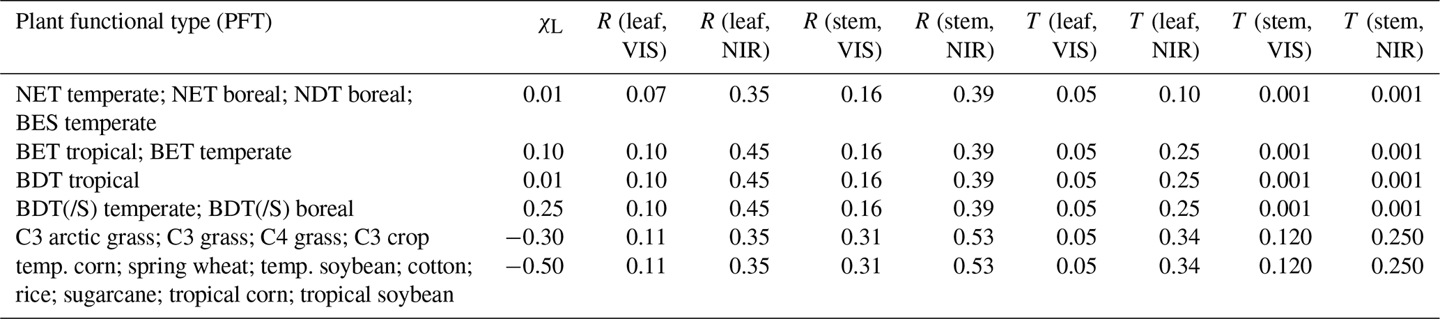
The following briefly describes the composition of the optical properties table used by today's CLM versions that is used as an example PFT classification in this paper. The SiB table by Dorman and Sellers (1989) was partly reused by Bonan et al. (2002) to suit the needs of the CLM (Table 1). Bonan et al. (2002) assigned properties of SiB table class 1, “broadleaf evergreen trees” (“BETs”), and SiB table class 2, “broadleaf deciduous trees” (“BDT”), for the CLM “BET tropical”, “BET temperate”, “BDT temperate”, and “BDT boreal”, “BDT tropical' and for PFTs containing “broadleaf deciduous shrubs” (BDS) (i.e., “BDS temperate” and “BDS boreal”). The leaf angle specification (as departure from the spherical distribution; χ_L, i.e., 1 = planophile, −1 = erectophile, and 0 = spherical) for both BET PFTs was set to 0.10, and for temperate and boreal BDTs and BDSs it was set to 0.25. However, for BDT tropical, the leaf angle was set 0.01. The SiB class 4 “needleleaf evergreen trees” (NETs) and class 5 “needleleaf deciduous trees” (NDTs) were used to form CLM PFTs “NET temperate” and “NET boreal”, “NDT boreal”, and “broadleaf evergreen shrubs (BESs) temperate”. SiB table class 7 “ground cover” was used to parameterize the optical properties of grasses and crops (χ_L of −0.30). However, in later CLM versions such as in CLM5 (Table 1), the optical properties of grass and crop PFTs were referenced to Asner et al. (1998), in which the estimates are presented only for spectral subsets following different satellite sensor bandwidths (e.g., AVHRR bands 1 (VIS, 550–700 nm) and 2 (NIR, 725–1100 nm)) and thus fail to represent full optical range. In addition, it is worth pointing out that the stem optical properties are defined based on dead leaf estimates reported by Dorman and Sellers (1989). Additional confusion may be caused by the fact that the SiB table by Dorman and Sellers (1989) defines the NIR region as 700–4000 nm, whereas in one of the SiB table source datasets (in Sellers, 1985) the respective wavelength region is defined as 700–3000 nm. It is noteworthy that the current standard of measuring spectral data extends only to 2500 nm. Although the spectral range used in this study does not cover the full theoretical range of total shortwave broadband albedo (300–4000 nm), the spectral range of 400–2400 nm contains ∼96 % of the total solar irradiation (Thuillier et al., 2003, Fig. 1) and thus suffices to approximate total VIS and NIR albedos. In addition, as the CLM table contains a column for χ_L, we assess their appropriateness based on measured and published data. In CLM5, the predefined angles (χ_L, Table 1) are 0.01 (∼59.7^∘) for both NETs, NDT boreal, BDT tropical, and BES temperate, 0.10 (∼56.6^∘) for BETs, 0.25 (∼51.3^∘) for BDT(/S) (refers to “BDT + BDS”) boreal and temperate, −0.3 (∼69.5^∘) for grasses and C3 crops, and −0.5 (∼75.5^∘) for other crops. As the focus of this paper is on optical properties, an extensive review of leaf angle literature is not attempted.

Table 1 Collapsed version of the CLM5 optical properties table in the CLM5 (2018) manual (Table 2.8). Note that in the CLM the leaf angle value (χ_L) is quantified based on divergence from spherical distribution: 1 = planophile, −1 = erectophile, and 0 = spherical. Reflectance (R) and transmittance (T) in VIS (< = 700 nm) and in NIR (> = 701 nm). “BDT(/S)” contains both BDT and BDS PFTs for temperate and boreal PFTs.

2.2 Spectral databases

The spectral repositories used in this study are openly available online archives that were selected based on their reputation and methods used to collect the data (e.g., device, spectral range, metadata availability). To reduce differences in data resulting from different instrumentation, we only used leaf- or needle-level data measured using an integrating sphere to get both leaf R_(λ) and T_(λ) information for forest and crop PFTs. For grasses “canopy-level” R_(λ) measurements were used (except for arctic grasses, for which the data were collected using leaf clip) (Table 2).

The Lopex93 and Angers datasets belong to a group of “foundational datasets” defined as “Previously published spectroscopic data and associated metadata resources that represent exemplary, historically-notable, or transformational collections for the environmental spectroscopy community” (EcoSIS, 2017). Lopex93 and Angers contains measurements of species with flat leaves, i.e., grasses, crops, broadleaf tree, and shrub species. The Lopex93 campaign was organized by the Joint Research Centre (JRC) in Italy during the summer of 1993 and contains leaf R_(λ) and T_(λ) data for leaves of 45 species. Angers is a dataset collected by the National Institute for Agricultural Research (INRA) in France in June 2003 containing R_(λ) and T_(λ) data for leaves from 39 species. For conifer needles few spectra are available due to obvious difficulties in measuring small needles. For boreal tree species two datasets are available by Lukeš et al. (2013) and Hovi et al. (2017) via SPECCHIO. For example, the dataset by Hovi et al. (2017) contains R_(λ) and T_(λ) data for 25 Eurasian and North American boreal tree species measured during peak growing season. These two datasets contain measurements of both sun-exposed and shaded leaves, by leaf sides (adaxial and abaxial) from different canopy positions. For temperate conifers we used the EcoSIS library from Serbin (2014) and data by Noda et al. (2014) stored in the Japan Long-Term Ecological Research Network (JaLTER) archive. The dataset by Serbin (2014) was collected in the north–central and northeastern United States (US) as part of NASA's Forest Functional Types Project (NNX08AN31G). The data from Noda et al. (2014) were measured in Japan with varying spectral ranges of 350–2500 nm and 350–2050 nm for foliage and bark. (Note that spectra are available for leaves and shoots for different canopy positions; for foliage, the R_(λ) and T_(λ) are provided separately for abaxial and adaxial sides.)

Table 2 Spectral data used in this study. This table only lists data properties that were used in this study (i.e., the datasets may contain other data collected using different devices or methods or from different targets). Abbreviations: IS – integrating sphere; LC – leaf clip; BF – bare optical fiber or optical head of spectrometer; R_(λ) – reflectance spectra; T_(λ) – transmittance spectra. Target BDT(/S) contains both BDT and BDS PFTs for temperate and boreal regions, and similarly “BET(/S)” contains both BET and BES PFTs.

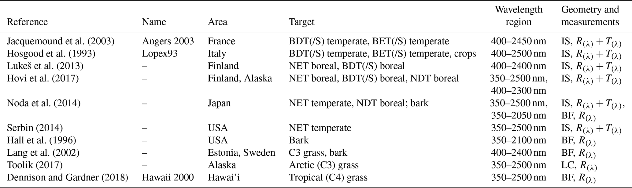
The bark R_(λ) dataset was compiled using spectra from Noda et al. (2014), Hall et al. (1996), and Lang et al. (2002). In addition to containing bark R_(λ) spectra, the Hall et al. (1996) dataset also includes measurements of branches, moss, and litter for boreal conditions (collected in the Superior National Forest of Minnesota US). However, in this study we used the dataset by Lang et al. (2002) to assess variation in R_(λ) of different C3 grass compositions because the spectral range of data from Lang et al. (2002) was larger than that of Hall's data. For arctic (C3) grasses we used EcoSIS data measured in Toolik, an arctic research field station in Alaska (Toolik, 2017). For tropical (C4) grasses we used the EcoSIS data “Hawaii 2000” dataset (Dennison and Gardner, 2018). In the absence of measured transmittance data for grasses, they were assumed to be equal (in S1 in the Supplement) with those of crops (and grasses) contained in the Lopex93 dataset.

2.3 Processing of the spectra

The spectra from different repositories were resampled to follow a constant spectral range and interval (i.e., the spectral range and measurement interval of different devices varies and must therefore be unified). Spectra were resampled to have a 1 nm interval within a spectral range of 400–2400 nm using the R package “Prospectr” (Stevens and Ramirez-Lopez, 2015). The spectral regions with extreme noise were either removed or replaced with local means before smoothing. If a 10 % smoothing (span of 0.10) was enough to repair noisy regions in the spectra, no removals or replacements were done. Smoothing was done using LOESS regression (R default package) applying nonparametric least squares regression for localized subsets. Note that spectra >2400 nm or <400 nm were removed in an effort to harmonize the spectral range of the different datasets (Table 2). Normalized (i.e., summed up to 1) solar irradiance (SI_(λ)) spectra were used to weight both R_(λ) and T_(λ) spectra before calculating the VIS (400–700 nm) and NIR (701–2400 nm) averages for R and T (i.e., all band averages of R_(λ) and T_(λ) are given after weighting with SI_(λ)). We used the white-sky SI_(λ) measured at sea level to account for atmospheric scattering and absorption effects (Fig. 1). The SI_(λ) was normalized (i.e., to sum up to 1) separately for VIS and NIR wavelength bands (i.e., the relative shape of the SI_(λ) within the VIS and NIR subset was preserved). Foliage SSA_(λ) was obtained as a sum of R_(λ) and T_(λ) (separately for VIS and NIR) and multiplied with the respectively (i.e., VIS or NIR) normalized SI_(λ). The leaf or needle SSA was obtained as a sum over the resulting VIS and NIR bands. The SI_(λ) normalization was adapted to the shorter NIR spectral ranges of the Hall et al. (1996), Hovi et al. (2017), and Noda et al. (2014) data (in Table 2). All VIS- and NIR-averaged R, T, and SSA values represented in this paper have been weighted with the SI_(λ) to show results consistently.

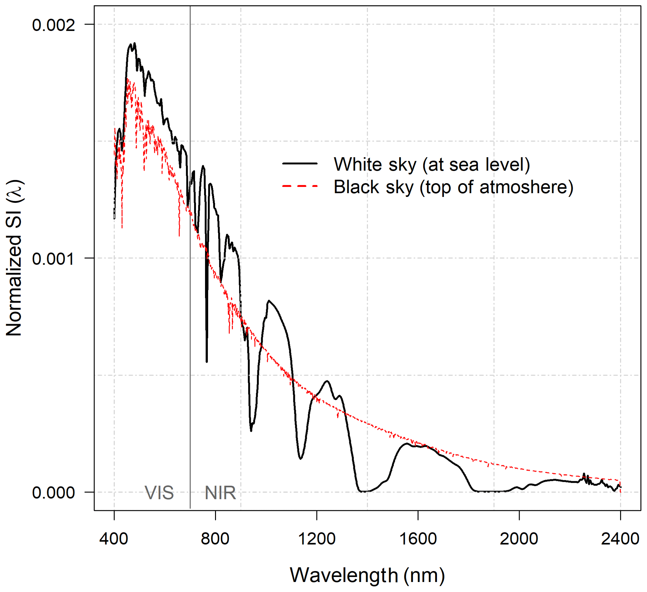
Figure 1 The normalized (i.e., summed to unity between 400 and 2400 nm) white-sky solar irradiance spectra (SI_(λ)) measured at sea level and, for reference, the normalized black-sky top-of-the-atmosphere spectra by Thuillier et al. (2003). The figure is shown to illustrate the effect of atmosphere on the shape of SI_(λ) (note that in our calculation the white-sky spectra were renormalized within VIS (400–700 nm) and NIR (701–2400 nm) subsets).

2.4 Upscaling spectra from needle to shoot

Clustering of needles into shoots causes the R and T of shoots to be systematically smaller than those of needles, due to within-shoot multiple scattering (Stenberg, 1996). By replacing the VIS and NIR SSA_needle with SSA_shoot, the systematic bias caused by shoot-level clumping can be accounted for in RT modeling. The spectra of needles can be upscaled to shoot level using spherically averaged silhouette to total needle area ratio (STAR; e.g., Oker-Blom and Smolander, 1988; Stenberg, 1996). For a shoot without within-shoot shadowing, the STAR would be 0.25 because the spherically averaged projection area of a convex needle is one-fourth of its total area (Lang, 1991). The STAR is known to vary between species and canopy positions (and may vary, e.g., from 0.12 to 0.28), and in the absence of adequate data the STAR can be approximated using a value of 0.16 for a range of shoot structures (Thérézien et al., 2007). In this study a constant STAR of 0.16 was used for all conifer species for demonstration. At shoot level the p is linearly related with STAR (i.e., $p=\mathrm{1}-\mathrm{4}\times$ STAR under diffuse radiation conditions), which allows upscaling the SSA(λ) (i.e., SSA${}_{\mathrm{needle}\left(\mathit{\lambda }\right)}=R_{\left(\mathit{\lambda }\right)}+T_{\left(\mathit{\lambda }\right)})$ to SSA_shoot(λ) (Smolander and Stenberg, 2003; Rautiainen et al., 2012) as the following Eq. (1):

$$\begin{array}{}\text{(1)}& {\mathrm{SSA}}_{\mathrm{shoot}\left(\mathit{\lambda }\right)}={\mathrm{SSA}}_{\mathrm{needle}\left(\mathit{\lambda }\right)}\left({\displaystyle \frac{\mathrm{1}-p}{\mathrm{1}-p{\mathrm{SSA}}_{\mathrm{needle}\left(\mathit{\lambda }\right)}}}\right).\end{array}$$

The SSA_shoot(λ) was multiplied with normalized SI_(λ) for VIS and NIR wavelength regions as explained in Sect. 2.3, and SSA_shoot in VIS and NIR were obtained by taking the sum over the spectra. Note that when STAR is greater than 0.25, then SSA_shoot > SSA_needle, which may happen if the shoot structure is abnormal (e.g., the shoot has very short needles which only cover the upper side of the twig (Thérézien et al., 2007)).

2.5 Leaf angle specification

Leaf angle distribution (LAD) of foliage determines radiation transmission though plant canopies and is also included in the CLM5 table (in a form of χ_L). The assumption on random foliage distribution remains valid for many conifer species (e.g., Barclay, 2001), and thus we focus on providing some example data for other PFTs. The leaf angle properties of PFTs will be defined based on data presented in Wang et al. (2007), Chianucci et al. (2018), Pisek et al. (2011), Gratani and Bombelli (2000), Zou et al. (2014), and Table I.6.2 in Ross (1981).

Wang et al. (2007) reported measured LIAs for three grass species (i.e., Andropogon gerardi, Panicum vigratum, and Sorghastrum nutans) measured in Konza Prairie in North America (data from Li, 1994) and for leaves of 38 species including flowering plants, shrubs, and trees measured in Ku-ring-gai Chase National Park in Australia (data from Falster and Westoby, 2003). The R library “RLeafAngle” (Wang et al., 2007) contains a dataset called “Falster” for 38 species published by Falster and Westoby (2003). The Falster data were used to obtain LIA estimates for “BDT(/S) tropical”. For “BDT(/S) temperate” and “BDT(/S) boreal” LIA estimates were obtained from data by Chianucci et al. (2018), which contain LIA measurements for 55 tree and shrub species collected by Pisek et al. (2013) and Raabe et al. (2015) at different sites in Sweden, Estonia, and the USA and for 83 species at various sites in central Italy. The mean LIA of “BET(/S) temperate” and “BET(/S) tropical” was approximated using two species from Hawai'i (i.e., Metrosideros polymorpha and Schizostachyum glaucifolium (bamboo) in Pisek et al. (2011) and two from the Mediterranian region (i.e., Phillyrea latifolia and Quercus ilex in Gratani and Bombelli, 2000).

The variety of mean χ_L or LIA estimates of different grass and crop species was demonstrated using data compiled by Ross (1981) from various sources and data from Li (1994) and Zou et al. (2014). As it is not easy to classify different plant species into either crop or grass, we chose to present these data by dataset (see S3 for details). The pure “grasses” (Li, 1994) and cool-temperate “crops” (Zou et al., 2014) data contained measured LIA estimates, but “crops + grass” data reported values using χ_L, which were converted to LIA in degrees (^∘). The conversion between mean LIA (θ_mean) and χ_L was approximated following the CLM5 (2018) manual as

$$\begin{array}{}\text{(2)}& \cos {\mathit{\theta }}_{\left(\mathrm{mean}\right)}={\displaystyle \frac{\mathrm{1}+{\mathit{\chi }}_{\mathrm{L}}}{\mathrm{2}}}.\end{array}$$

For each PFT the mean LIA estimates in degrees and as dispersion from a spherical distribution (χ_L) were obtained as an average across-species mean (species level data listed in S3). The species-mean LIA estimates were assigned to classic LAD types (de Wit, 1965) using the RLeafAngle-package function “selectClassic()” and thus may differ from that presented in the original works.

3 Results

3.1 Forest PFTs

3.1.1 Optical properties of forest PFTs

R and T of conifer needles were similar in NET temperate and NET boreal in both VIS and NIR wavelengths (Fig. 2, Table 3). For example, for NET temperate mean R_VIS was 0.08, and mean T_VIS was 0.04, and for NET boreal the respective values were 0.09 and 0.05. Similarly, for NET temperate (NET boreal) the mean R_NIR was 0.41 (0.41) and mean T_NIR was 0.31 (0.33). Thus, the CLM default R_VIS and T_VIS (0.07, 0.05) for NET appear appropriate (Table 1, Fig. 2a). However, the CLM default R and T in NIR are not at the correct level: the CLM defaults for R_NIR and T_NIR are 0.35 and 0.10, but based on our data the values should be ∼0.41 and ∼0.32, respectively (Figs. 2a, 3a).

The mean R and T were also similar for temperate and boreal BDTs (Table 3). For BDT temperate, the mean R_VIS was 0.08 and mean T_VIS was 0.06, and for BDT boreal, the respective values were 0.09 and 0.05. Similarly, for BDT temperate the mean R_NIR was 0.42 and mean T_NIR was 0.43, while for BDT boreal the respective values were 0.40 and 0.42 (Fig. 3b). Thus, we can conclude that the CLM for BDT R_VIS and T_VIS are appropriate (R_VIS=0.10 and T_VIS=0.05) (Fig. 2b). However, the CLM default value for BDT temperate and boreal T_NIR of 0.25 requires an update: based on our data the respective T_NIR should be and ∼0.43. For R_NIR the CLM default is 0.45 and the mean measured value was ∼0.41.

For BET temperate, the averages of R_VIS and T_VIS were 0.11 and 0.06, respectively (Fig. 3c, Table 3). These values corresponded well with the CLM default values (i.e., R_VIS=0.10 and T_VIS=0.05). However, the CLM default T_NIR of 0.25 was slightly smaller than the mean measured T_NIR of 0.33 (Fig. 2b). The CLM default BET R_NIR of 0.45 corresponds well with the measured mean R_NIR of 0.46.

Results showed that the CLM optical properties for NDT boreal are fine in VIS (Fig. 2a). However, CLM defaults for R_NIR and T_NIR of 0.35 and 0.10, were found to be too low – The R_NIR and T_NIR should be ∼0.39 and ∼0.42 based on measured data (Fig. 3d). It is noteworthy that the NDT boreal optical properties are more similar in NIR with BDT than with NET, which is the CLM default grouping (Fig. 2a, b).

Based on our calculation, the SSA_shoot is on average 32 % smaller in VIS and 10 % smaller in NIR than the SSA_needle (Tables 3, S2). The largest differences between the two albedo proxies resulted in a 36 % difference in VIS and a 15 % difference in NIR, with the smallest differences being 29 % in VIS and 7 % in NIR.

Figure 2 Leaf reflectance and transmittance in VIS (400–700 nm) and NIR (701–2400 nm) for different PFTs. Single species values are plotted to demonstrate the within- and between- PFT variation for (a) NET temperate and NET boreal, NDT boreal, (b) BDT temperate and BDT boreal, BET temperate, and (c) crops + grasses. The CLM default optical properties are plotted using large symbols.

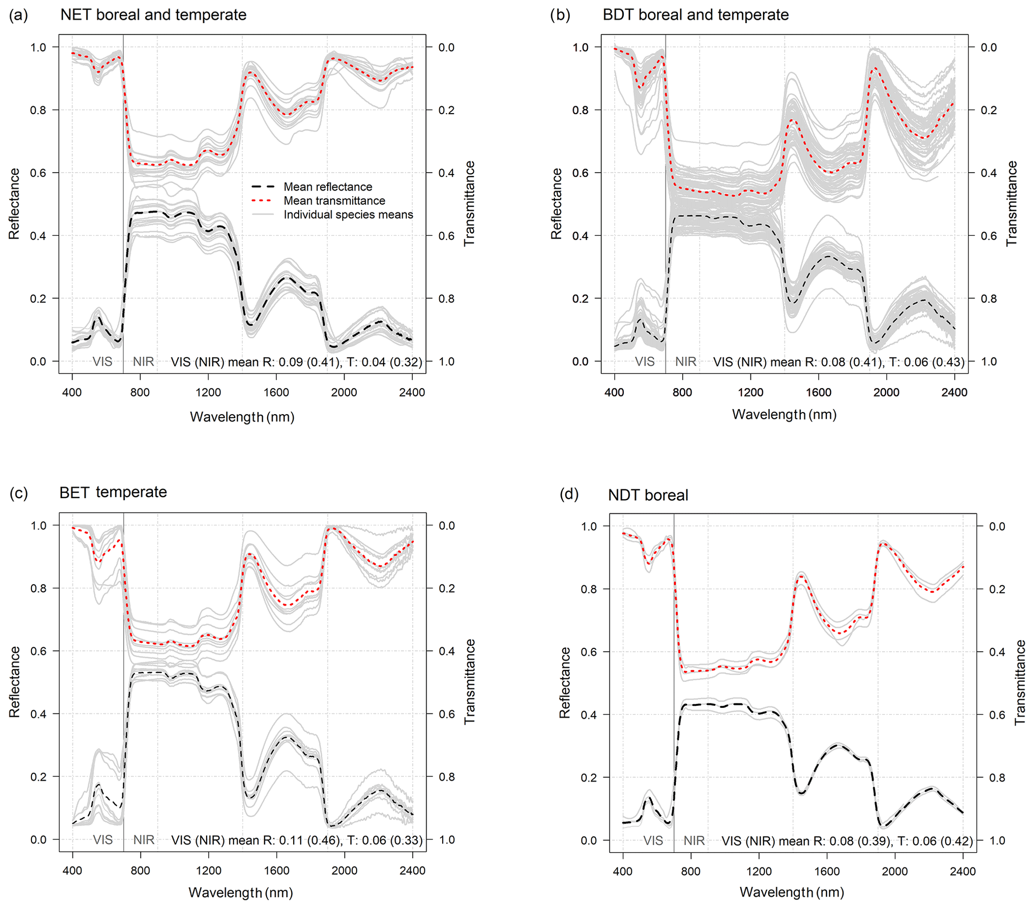
Figure 3 Average reflectance (R_(λ)) and transmittance (T_(λ)) spectra of foliage for forest plant functional types (PFTs) for n species samples: (a) NET boreal and temperate (n=18), (b) BDT boreal and temperate (n=54), (c) BET temperate (n=10), and (d) NDT boreal (n=4). Individual-species-mean R_(λ) and T_(λ) spectra are shown using light gray lines and are used to represent the within-PFT deviation in mean spectra (see individual species estimates in S2). The mean R_(λ) and T_(λ) for VIS (400–700 nm) and NIR (701–2400 nm) wavelengths are provided at the bottom of the images and are calculated as an average of the species means. Note that all VIS and NIR averages of R_(λ) and T_(λ) were weighted with solar irradiance spectra (SI_(λ)).

Table 3 Average leaf or needle reflectance (R), transmittance (T), single scattering albedo (SSA), and single scattering albedo corrected for shoot-level clumping (SSA_shoot) over VIS (400–700 nm) and NIR (701–2400 nm) wavelength regions by plant functional type (PFT). Note that all VIS and NIR averages of R_(λ) and T_(λ) were weighted with solar irradiance spectra (SI_(λ)). Standard error is given inside parentheses.

3.1.2 Optical properties of tree bark

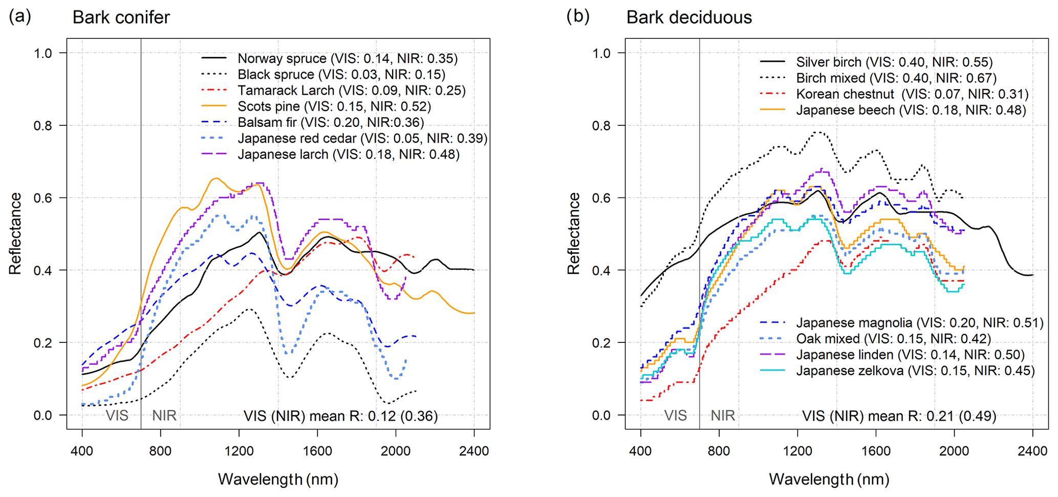
Figure 4 Bark reflectance (R_(λ)) of (a) coniferous, and (b) deciduous species in VIS (400–700 nm) and NIR (701–2400 nm) wavelength regions. The mean bark reflectance values in VIS and NIR are provided at the bottom of the images and are calculated as an average across the species mean (the mean across all bark values R_VIS=0.17 and R_NIR=0.43). Note that all VIS and NIR averages of R_(λ) and T_(λ) were weighted with solar irradiance spectra (SI_(λ)).

Based on our data sample, coniferous bark R_VIS varied between 0.03 and 0.20 and R_NIR varied between 0.15 and 0.52 (Fig. 4a, S2). The average coniferous bark R_VIS was 0.12 and R_NIR was 0.36. For deciduous species, the bark R_VIS varied between 0.07 and 0.40 and R_NIR varied between 0.31 and 0.67 (Fig. 4b). The average deciduous species bark R_VIS and R_NIR were 0.21 and 0.49, respectively. In the CLM, the same constant stem reflectance is used for all forested PFTs (R_VIS of 0.16 and R_NIR of 0.39). Thus, the CLM default bark reflectance in VIS and NIR falls within the range of measured values (average over all species R_VIS=0.17 and R_NIR=0.43). However, alternatively bark reflectance could be defined separately for coniferous and deciduous PFTs.

3.2 Optical properties of grass and crop PFTs

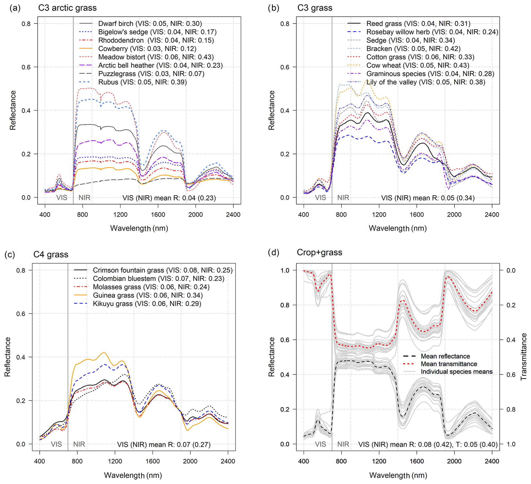
Figure 5 Optical properties of grasses and crops. Reflectance (R_(λ)) of (a) C3 arctic grasses, (b) C3 grass canopies, (c) C4 grass canopies, and (d) and transmittance (T_(λ)) of leaves of different crops (n=21, contains also some grass species): individual-species-mean R_(λ) and T_(λ) are shown using light gray lines and are used to represent within-PFT deviation in mean spectra (see individual species values in S2). The mean R and T for VIS (400–700 nm) and NIR (701–2400 nm) wavelengths are provided at the bottom of the images and are calculated as an average across-species means. Note that all VIS and NIR averages of R_(λ) and T_(λ) were weighted with solar irradiance spectra (SI_(λ)).

Leaf reflectance spectra for different grass species demonstrate large within-PFT variation, which exceeds the differences between various grass PFTs (i.e., C4, C3 arctic, and C3 grasses). The leaf mean R_VIS (T_VIS) of different grass and crop types (i.e., C3 arctic grass, C3 grass, C4 grass, and crops) were 0.04 (0.23), 0.05 (0.34), 0.07 (0.27), and 0.08 (0.42), respectively (Fig. 5., Table S2). In the CLM table, the leaf default R_VIS and R_NIR are 0.11 and 0.35 for all grass and crop PFTs. The CLM default leaf R_VIS seems a little high as only 3 of 42 grass or crop species (i.e., garden lettuce, corn, and soybean) reach the R_VIS of 0.11. The R_NIR of 0.35 on the other hand stands out like an outlier (Fig. 2c, Table S2), and thus a slightly higher value could be used. For crops, the measured mean leaf T_VIS and T_NIR were 0.05 and 0.40, respectively. Thus, although the measured leaf T_VIS values aligned perfectly with the CLM default value (of 0.05), the CLM default leaf T_NIR value of 0.34 needs an update. The updated leaf R_VIS and R_NIR could be ∼0.05 and ∼0.28 for grasses and ∼0.08 and ∼0.42 for crops (S2). In the absence of measured transmittance data for grasses, the T_VIS and T_NIR of grasses could be defined based on respective crop values (i.e., 0.05 and 0.40).

3.3 Leaf angle specification

Based on measured data, the mean LIA of BDT tropical (χ_L of 0.20 i.e., ∼52.1^∘) was found more planophile than what is the CLM default value of 0.01 (χ_L, i.e., ∼60^∘) (Tables 4, S3). However, as there is a lot of variation among LIA estimates between species (i.e., χ_L ranges from −0.42 to 0.84), the assumption of spherical foliage orientation seems fine for BDT(/S) tropical. For BDT(/S) temperate/boreal the mean LIA across species means was 36.0^∘ (i.e., χ_L of ∼0.59) and thus was also found to be more planophile than the CLM5 default of ∼51.3^∘ (i.e., χ_L of 0.25). Consequently, the χ_L value of BDT(/S) temperate/boreal could be adjusted to correspond better with observed variation in the data. For BET(/S) temperate/tropical the mean LIA was 48.5^∘ (i.e., χ_L of 0.32) and thus somewhat agreeing with the CLM5 default of ∼56.6^∘ (χ_L of 0.10).

Table 4 Mean leaf inclination angles (LIAs) of different flat-leaved plant functional types (PFTs). The angles are provided both in degrees (^∘) and as departures from a spherical distribution (χ_L). Number of observations is shown in column “n”. Individual species estimates are presented in Table S3.

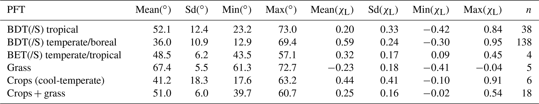
For the non-forest PFTs (i.e., grasses and crops), the CLM5 default parameterization of χ_L was either −0.30 (∼69.5^∘) or −0.50 (∼75.5^∘) depending on vegetation type. Based on measured data the mean χ_L of grasses (of −0.23, ∼67.4^∘) was found to correspond well with the CLM5 default value. However, for crops the observed χ_L values were clearly leaning towards more planophile (e.g., 41.2 and 51.0^∘, χ_L of 0.44 and 0.25) than erectophile foliage orientation (i.e., ∼75.5^∘, χ_L of −0.5). Cool-temperate crops demonstrated the largest variation in LIAs (ranged from 17.6 to 63.2^∘, i.e., χ_L from of −0.10 to 0.91). It is noteworthy that from among 29 grass and crops species, none reached χ_L of −0.50; however, two grasses had χ_L of −0.40 (Tables 4, S3). Thus, based on the data shown in this study, the CLM5 default χ_L of crops should be updated. The mean χ_L of the crop species presented here was 0.30 (∼48.5^∘) (S3).

4 Discussion

Based on a dataset compiled following a synthesis and harmonization of spectral data found in a variety of data repositories, we showed that many optical properties based on the SiB table (currently used by, e.g., the CLM) are in need of an update. While the optical properties were by default at the correct level in the VIS wavelength region (determines vegetation productivity via photosynthesis), the changes in optical properties in the NIR wavelength region may be expected to have an impact on predicted surface albedo. To our knowledge, only Göttlicher et al. (2011) have made an attempt to verify the CLM optical parameters of BET tropical (PFT) using measured spectral data. However, as their NIR data covered only a part of the spectrum (from 701 to 1300 nm), only VIS verification was obtained. We cannot argue that the values presented in this paper are the “truth” per se, nor that researchers should use the values presented in this paper. However, we can state that there are systematic biases in the optical property values in the NIR wavelength region, across all PFTs. For example, for NET and NDT, the empirically based SSA_needle values exceeded the CLM default parameters by 62 % and 78 %, respectively; even after accounting for shoot-level clumping, the SSA_shootNIR was still 44.4 % (NET) and 64.4 % (NDT) larger than the CLM defaults. Similarly, for the BDT, BET, and crop PFTs, the measured leaf SSA_NIR values were 20.0 %, 14.3 %, and 18.8 % larger than the CLM default estimates, respectively (numbers calculated based on S2). It is noteworthy that as LSMs are often run using PFT distributions obtained from remotely sensed land cover products and as there are no possibilities for within-PFT species differentiation, the use of a constant shoot-structural factor to upscale SSA_needle to SSA_shoot may be justified. However, for other applications having species information readily available, the species-specific shoot structural factors should be used. According to Rautiainen et al. (2012), SSA_shoot are considerably smaller than SSA_needle, and there is more variation in shoot spectra (coefficient of variation, CV, 8 %–21 %) than in the needle spectra (CV 2 %–13 %) due to the geometry of the shoot. In this study, the SSA_shoot in VIS and NIR was ∼30 % and ∼10 % smaller, respectively, than the SSA_needle (note that a constant factor was used).

As optical properties represent the effective surface variables, we can argue that there is a need to update the parameters, as changes in initial parameterization may be expected to result in changes in predicted surface albedo. However, whether or not (and if yes, then to what extent) changes in optical properties result in changes to predicted surface albedo requires LSM simulations since LSMs have been tuned to reduce influences of identified biases and possible compensating errors. For example, in the case of the CLM, no global soil reflectance dataset was available during model development and soil reflectance data are now based on the tuning of the CLM-simulated surface albedo to match MODIS observations (Lawrence and Chase, 2007). While this may not be too important in dense canopies with high LAI, in sparse canopies (LAI<2) soil reflectance becomes more important. In addition, we must consider that the major assumptions of 1-D RT models themselves are likely to source some error: the CLM employs a simplified plane-parallel, two-stream model based on the homogenous turbid medium assumption with isotropic scattering properties. One-dimensional models commonly ignore stems and branches, but the stems are accounted for by the CLM RT model: optical parameters are calculated as a weighted average of leaf and stem areas (i.e., LAI and stem area index, SAI). This may introduce possible errors (or biases) because (i) empirical data and the theoretical basis for a more accurate definition of SAI are currently lacking (e.g., the CLM5 manual, Sect. 2.29.5.2 (CLM5): “The existing CLM(CN) algorithm sets the minimum SAI at 0.25 to match MODIS observations, but then allows SAI to rise as a function of the LAI lost, meaning than [sic] in some places, predicted SAI can reach value [sic] of 8 or more. Clearly, greater scientific input on this quantity is badly needed.”) and (ii) incompatibilities in vegetation structural descriptions in the RT models employed (i.e., MODIS LAI is based on 3-D RT model, whereas the CLM employs 1-D RT model), which may lead to erroneous assessments of the absorbed, transmitted, and reflected fluxes (Pinty et al., 2004, 2006). It is noteworthy that we did not provide updated optical property values for the stems of grasses and crops due to the scarcity of measured spectral data for these plant components. However, considering that information on SAI is currently lacking and that grass and crop stems are ignored by today's RT models employed in vegetation remote-sensing applications (e.g., the MODIS LAI algorithm (Knyazikhin et al., 1999) and PROSAIL (Jacquemoud et al., 2000)), optical properties of grass and crop stems could also be ignored in CLM RT simulations to correspond better with MODIS LAI.

Generally speaking, the need for improving the RT models employed in LSMs has been acknowledged, and progress has already been made (Yuan et al., 2017; McGrath et al., 2016). For example, a “domain-averaged structural factor” (i.e., effective LAI accounting for inhomogeneous horizontal distribution such as tree clumping and canopy gaps) and multilayer canopy vertical albedo profile were recently added by McGrath et al. (2016) for the ORganising Carbon and Hydrology In Dynamic EcosystEms (ORCHIDEE, SVN r2566) model. In their approach, tree crowns were treated as spheroids filled with turbid medium with infinitely small scatterers, and tree trunks were ignored as spectral parameters are extracted from remote-sensing data without differentiation between leafy and woody areas. However, as a pgap model (Haverd et al., 2012) accounts for tree trunks in canopy gap parameterization, the trunks should ideally also be accounted for as canopy spectral parameters are determined (Naudts et al., 2015; McGrath et al., 2016). They modeled grasses and crops as homogenous blocks, without internal structure, and defined the tunable “correction factor” to account clumping effects. For the CLM, recent advancements were done by Yuan et al. (2017), who compared four representative 1-D RT models under the same framework and implemented the appropriate modifications for the CLM4.5 (Oleson et al., 2013). They proposed changes for the employed LAD equation and two modifications following the paper by Pinty et al. (2006) regarding the treatment of incident diffuse radiation and backward scattering coefficient for incident direct radiation.

As an alternative for empirically based correction factors, which may potentially violate the law of energy conservation, new perspectives for the old challenge are offered by the theory of spectral invariants: based on spectral invariants theory, SSA(λ) is the only parameter that depends on wavelength, while all other parameters are determined by canopy structural factors (Wang et al., 2018). In this paper, we demonstrated how information on shoot geometry (i.e., p) can be used to upscale SSA_needle(λ) into effective SSA_shoot(λ) to account for within-shoot scattering, which violates the basic assumptions behind the RT calculation (i.e., nonrandom ordering of finite-sized needles). The proposed correction, is not currently accounted for in LSMs and (i) can be incorporated by simply replacing SSA_needle with effective SSA_shoot in the RT calculation, (ii) is applicable to RT models employing turbid media assumption and Beer's law, and (iii) provides the simplicity required by LSMs. In addition to spectral invariants theory being already incorporated into the MODIS LAI algorithm (Knyazikhin et. al., 1999), other desirable features from the point of LSM are that p (i) allows the generation of consistent products from satellite sensors operating at different spatial resolutions (Ganguly et al., 2008a) and (ii) permits compressing 3-D information into 1-D form across various spatial domains (Ganguly et al., 2008b) and (iii) allows measuring, scaling, and validation (Stenberg et al., 2016). As remotely sensed products are used as an input in LSMs, advances in RT modeling employed in remote sensing should ideally be reflected by LSM RT parameterizations. In addition, more effort in LSM RT modeling is needed for developing scaling routines to account for seasonal changes in optical properties (and SAI), and for improving parameterizations for snow and ice (Yuan et al., 2017).

PFT definitions are needed by LSMs to classify species into groups of similar structural and functional characteristics. While that appears a relatively simple task, this is not always the case. For example, while the difference between a tree and a shrub might seem easy to define, in practice defining these two is complicated by overlapping definitions. While both trees and shrubs are perennial woody plants, a shrub is considered shorter in stature than a tree and typically has more stems. However, a shrub may have as few as one stem and be tall in stature (up to 3 or 4 m in height) analogous to a small tree. Thus, the optical properties of shrub PFTs could be defined based on respective forest PFTs optical properties. In practice, we suggest that optical properties of, e.g., BES temperate be based on BET tropical and BET temperate instead of on NET temperate/boreal and NDT boreal optical properties, which is the default CLM grouping. In addition, as the optical properties of the NDT boreal are more like those of BDT (especially in NIR) than NET, which is the current CLM default grouping, the CLM could classify NDT into the BDT group rather than NET. Further, regarding the PFT boundaries, here we classified English ivy as belonging to BET(/S) temperate/boreal, despite it being an evergreen vine and bamboo as BET(/S) temperate/tropical (as it can reach up to 15 m height and has flat-leaf structures), although it is a flowering plant rather than a tree or shrub. In addition, the dataset by Chianucci et al. (2018) contained two plants belonging to the grass family and one fern species, but as their growth form was recorded as tree or shrub, we decided to keep them in the data.

Many of today's land surface models such as JSBACH (JSBACH, 2019), JULES, and ORCHIDEE assume LAD to be spherical. However, the assumption of spherical LAD has been found to cause significant underestimation of light transmission (Stadt and Lieffers, 2000) and has been found to be invalid for most temperate and boreal deciduous tree species based on an extensive dataset of measured LADs (Pisek et al., 2013; Chianucci et al., 2018) (e.g., only 14 of 138 species the LAD was spherical). Another study with Australian species showed that only 3 of 12 types of herbaceous plant canopies and 8 of 38 plant species (e.g., trees, woody shrubs, climbers, ferns, and cycads) had spherical LAD (Wang et al., 2007). Note that these two datasets were also used in this study. In the CLM the LAD definition denotes the departure from a spherical distribution: based on results, the CLM default LAD definition of forested PFTs could be slightly more planophile. For LSMs which can implement nonspherical LAD definitions, LAD parameters for a range of species are readily available from Chianucci et al. (2018) and Wang et al. (2007). However, the finding that CLM5 default LAD for crops is notably too vertical (i.e., the CLM5 default crop χ_L stands out as an outlier from among the empirical observations) requires attention from modelers. We acknowledge that while LAD may be assumed to be a species-specific parameter, it may be hard to estimate correctly as it changes based on plant development stage (e.g., crops) and as a response to solar illumination conditions (i.e., dual role of being exposed for solar radiation to enable photosynthesis but to avoid overexposure, which would cause heat stress). Thus, future studies are needed to address the issue of the PFT LAD definition, especially in the case of grasses and crops that are more exposed to solar radiation than trees. As an alternative to field measurements, LAD may also be inverted based on remotely sensed data (Huang et al., 2006).

In the future, large databases which systematically collect chemical and spectral data at different scales (i.e., from leaf to canopy level) and standardized protocols for field and lab work may be expected to become more common (e.g., Asner and Martin, 2016). While the motivation of remote-sensing scientists is to build these databases to foster scientific discoveries, the same databases could also be used to provide inputs for different LSMs (especially those employing plant traits). The build-up of larger databases would solve most present-day problems in terms of data usability by providing standardized data access policies, data formats, preprocessing, and metadata. We should aim for a truthful description of vegetation properties in different LSMs, as that is a prerequisite for increasing the accuracy of the predictions.

5 Conclusions

Using the CLM PFT grouping as an example, we found that the default PFT optical parameters fell within the range of measured values in the VIS band, but in the NIR band updates are needed. Such updates may be expected to have a direct impact on the modeling of surface albedo and the shortwave radiation balance and, in turn, on fluxes of CO₂, moisture, and energy at the surface. Thus, we encourage modelers employing two-stream RT approximations based on leaf-level optical properties to check their models' default optical property parameters and consider using shoot-level clumping-corrected values for NET and NDT.