A predictive algorithm for wetlands in deep time paleoclimate models

Methane is a powerful greenhouse gas produced in wetland environments via microbial action in anaerobic conditions. If the location and extent of wetlands are unknown, such as for the Earth many millions of years in the past, a model of wetland fraction is required in order to calculate methane emissions and thus help reduce uncertainty in the understanding of past warm greenhouse climates. Here we present an algorithm for predicting inundated wetland fraction for use in calculating wetland methane emission fluxes in deep-time paleoclimate simulations. For each grid cell in a given paleoclimate simulation, the algorithm determines the wetland fraction predicted by a nearest-neighbour search of modern-day data in a space described by a set of environmental, climate and vegetation variables. To explore this approach, we first test it for a modern-day climate with variables obtained from observations and then for an Eocene climate with variables derived from a fully coupled global climate model (HadCM3BL-M2.2; Valdes et al., 2017). Two independent dynamic vegetation models were used to provide two sets of equivalent vegetation variables which yielded two different wetland predictions. As a first test, the method, using both vegetation models, satisfactorily reproduces modern day wetland fraction at a course grid resolution, similar to those used in paleoclimate simulations. We then applied the method to an early Eocene climate, testing its outputs against the locations of Eocene coal deposits. We predict global mean monthly wetland fraction area for the early Eocene of 8×10⁶ to 10×10⁶ km² with a corresponding total annual methane flux of 656 to 909 Tg CH₄ yr⁻¹, depending on which of the two different dynamic global vegetation models are used to model wetland fraction and methane emission rates. Both values are significantly higher than estimates for the modern day of 4×10⁶ km² and around 190 Tg CH₄ yr⁻¹ (Poulter et al., 2017; Melton et al., 2013).

1 Introduction

Methane (CH₄) is a powerful greenhouse gas. As well as absorbing infrared radiation from the Earth's surface, it also contributes to additional indirect warming through its photochemistry and oxidation to CO₂ in the atmosphere (IPCC, 2013). Along with other trace gases, methane is therefore an important component of the Earth's climate system; but for studies of the past, such as warm greenhouse paleoclimates, we lack suitable geochemical or biological proxies for methane concentration. Therefore, Earth system models used to reconstruct ancient climate or develop future climate scenarios must either assume atmospheric methane concentrations as a boundary condition and/or incorporate dynamic methane fluxes from natural sources and sinks (Beerling et al., 2011). The main natural source of methane is wetland environments via microbial action in anaerobic conditions (Whiticar, 1999), but methane fluxes from wetlands are also modulated by climatic factors such as temperature (Westermann, 1993). Therefore, in order to model fluxes of methane to the atmosphere both the extent and locations of wetlands need to be known. For the modern day, recent past and near-future scenarios, maps of observed wetland extent (Prigent et al., 2007; Papa et al., 2010; Schroeder et al., 2015; Poulter et al., 2017) can be used or wetland extent can be calculated at a sub-grid level from fine-resolution topographical data (as in the TOPMODEL approach of Beven and Kirkby, 1979; Lu and Zhuang, 2012; Stocker et al., 2014), as wetlands only form where the ground is relatively flat.

For the study of deep-time paleoclimates (many millions of years in the past) there are no direct observations of wetland extent, although we may use a proxy such as coal deposit locations as we discuss in Sect. 3.2.1, and the topography is only known on relatively coarse resolutions of around 0.5^∘ at best. Therefore, any model calculation of wetland extent must either rely on using approximate knowledge of the topography or not rely on the topography at all. Previous studies (Beerling et al., 2011; Valdes et al., 2005), the only current model-based approach for deep-time paleoclimates, classified grid cells as either producing or not producing methane, based on either (i) a month being within a defined melt season for grid cells where mean monthly temperature drops below 0 ^∘C for at least 1 month of the year, or (ii) precipitation being greater than evapotranspiration. They then scaled emissions by empirically derived functions of the variance or standard deviation of orography at the best resolution available. The scaling effectively reduces methane emission rates in grid cells where elevation varies significantly and are therefore unlikely to have substantial wetlands within them, but relies on what may be quite coarse-resolution topography not able to resolve sub-grid-scale variations. The goal of this paper is to explore other methodologies for calculating wetland extent in the context of a deep-time paleoclimates.

In this work we develop a nearest-neighbour-based algorithm to predict the fraction of a specified area that is wetland (FW). We base this on a modern-day reference data set of FW and corresponding environmental variables, empirically associating the FW observations with corresponding observed climate data and vegetation data calculated using one of two dynamic global vegetation models (DGVMs), the Sheffield Dynamic Global Vegetation Model (Woodward et al., 1995; Beerling and Woodward, 2001) and the Lund-Postdam-Jenna model (Wania et al., 2009). Wetland is defined in the same manner as for our reference data (Poulter et al., 2017), discussed in the following section. It includes both permanently and seasonally flooded soils but excludes lakes, reservoirs, rivers, areas of rice cultivation, saline estuaries and salt marshes. We demonstrate its application by predicting FW and CH₄ fluxes for an early Eocene (52 Ma) model climate, an interval of greenhouse warming (Zachos et al., 2008) when sedimentary records indicate the existence of large areas of wetlands (Sloan et al., 1992; Beerling et al., 2009). For the Eocene, the same climate variables are obtained from a fully coupled global climate model and vegetation variables are derived from the same DGVMs. We then predict FW for the Eocene by analysis and comparison to the modern-day reference data. We note that different reference sets, vegetation models or climate models will likely yield different results and these should be explored in future work; but our aim here is to demonstrate this approach and its potential rather than to produce a model–model intercomparison.

In the “Data and methods” section we first describe modern-day wetland data at 0.5^∘ spatial resolution and a monthly time step for a mean modern-day year, along with climate and vegetation data which we later use as a reference data set. We then describe two test data sets at lower spatial resolution, equivalent to that used in paleoclimate models, again for a single year. The first of these is for the modern day and derived by interpolation of the reference data, and the second is derived from a paleoclimate model of the early Eocene. We briefly describe unsuccessful attempts to model FW through analysis of the reference data set. The main conclusion of these unsuccessful attempts being to indicate that any relationship between FW and various environmental variables must be quite complex. We then introduce the nearest-neighbour method we later found to be successful and finally in that section describe the model used to calculate wetland methane emissions.

In the “Results and discussion” section we first discuss model results for the modern-day test data set where we expect the nearest-neighbour method should perform well, since the test data are simply a version of the reference data interpolated to lower spatial resolution; these results, therefore, serve to demonstrate whether or not some form of the nearest-neighbour method could be successfully applied to prediction of FW for a climate very different to the modern day. We then apply this method to prediction of FW for the Eocene, and show that we can tune it by using the locations of coal deposits as wetland proxies.

2 Data and methods

2.1 Modern-day reference data

We use a modern-day reference data set of observed FW, the term observed being used to distinguish this from our later model results, with corresponding environmental data to develop an algorithm for the prediction of FW in the past, i.e. we assume that there exists a relationship between FW and the environmental variables compiled in the reference data and then apply that relationship to predicting FW in the past. We use the recently developed SWAMPS-GLWD (Poulter et al., 2017), which improves on the Surface Water Microwave Product Series (SWAMPS; Schroeder et al., 2015) using the static inventory of wetland area from the Global Lakes and Wetlands Database (GLWD; Lehner and Doll, 2004), correcting the SWAMPS data set in regions where this satellite-derived data set fails to detect water beneath closed canopies. We calculated the average monthly FW at each 0.5^∘ × 0.5^∘ grid cell for the years 2000 to 2012 on a monthly time step to give a modern-day FW (FW_obs; annual max shown in Fig. 1). Corresponding climate data on the same spatial and temporal resolution were obtained from CRU-NCEP v4.0 (Wei et al., 2014) and averaged to give monthly values for a mean modern-day year over the same time interval. The climate data for this mean year were then used to drive two DGVMs: the Sheffield Dynamic Global Vegetation Model (SDGVM; Woodward et al., 1995; Beerling and Woodward, 2001) and the Lund-Postdam-Jenna model (LPJ; Wania et al., 2009) to produce corresponding vegetation data. The combination of these yielded a reference data set of FW, climate (temperature and precipitation) and vegetation (leaf area index, net primary productivity, transpiration, evapotranspiration, soil water content and surface runoff) variables (either SDGVM or LPJ) for a set of 0.5^∘ × 0.5^∘ spatial and monthly temporal resolution sites for a single modern-day average year. Some variables, such as transpiration and evapotranspiration, are available from both climate and vegetation models. In such cases we use those from the vegetation model as they will be calculated from a more advanced vegetation scheme. To ensure that wetlands in areas dominated by agriculture or areas where one of our vegetation models, SDGVM, predicts bare land did not bias our FW predictions, such grid cells were removed from the reference data. For the latter, this was done simply by removing those grid cells that SDGVM predicted to be bare land. For the former, we removed those that were 50 % or more, by cover, classed as cultivated and managed or mosaic cropland (Global Land Cover 2000 database, 2003).

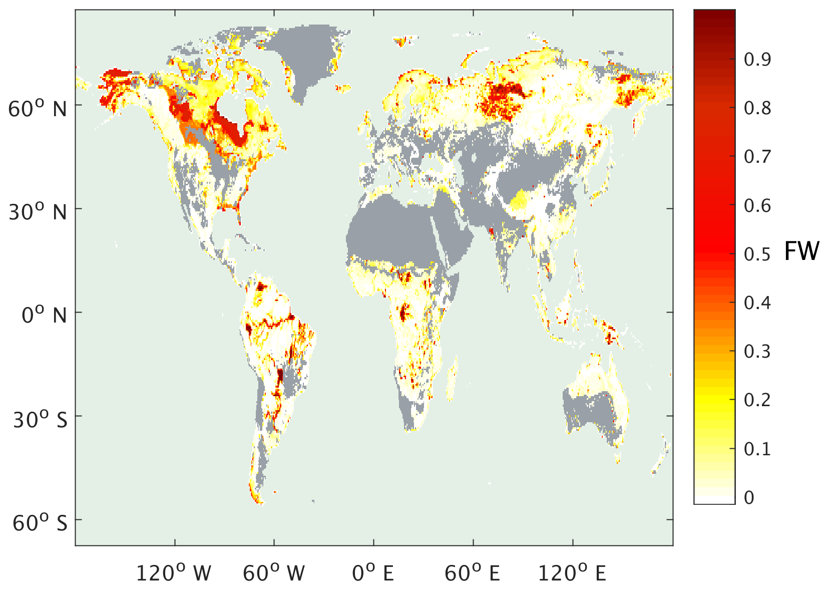
Figure 1 Annual monthly maximum observed FW from the SWAMPS-GLWD data set (Poulter et al., 2017), mean of 2000 to 2012. Grey shading indicates bare land, as predicted by SDGVM, or >50 % cultivated (Global Land Cover 2000 database, 2003).

Many of the methods that can be used to analyse the reference data and predict FW require that the data are scaled so that each variable covers a similar range of values. Therefore, we scaled the values of each environmental variable, X, using their global mean, μ_x, and global standard deviation, σ_x, i.e. for a given grid cell, J, each variable was scaled as

$$\begin{array}{}\text{(1)}& X^{\prime }\left(J\right)={\displaystyle \frac{X\left(J\right)-{\mathit{\mu }}_x}{{\mathit{\sigma }}_x}}.\end{array}$$

This scales all variables such that they have a global mean of 0 and standard deviation of 1.

2.2 Test data sets

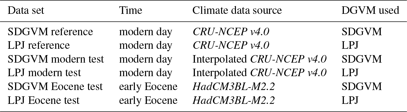
A modern-day test data set was made by interpolating the reference climate data to 2.5^∘ × 3.75^∘, the spatial resolution often used for paleoclimate models. The DGVM simulations were driven by this interpolated data to yield the vegetation outputs. All climate and vegetation variables were scaled in the same way as the reference data, using the global means and standard deviations of the reference data. The paleoclimatic assessment of our model was performed using an early Eocene test data set made using a single year of output, on a monthly time step, from a three-dimensional fully dynamic coupled ocean–atmosphere global climate model HadCM3BL-M2.2 (Valdes et al., 2017), on a 2.5^∘ latitude by 3.75^∘ longitude grid. To simulate the early Eocene a Ypresian paleogeography and high CO₂ concentration (4 times modern; 1120 ppm; Anagnostou et al., 2016) was used. SDGVM and LPJ were both run with these model-simulated climate data to produce the vegetation variables required, as was done for the reference data set, whereas temperature and precipitation were derived directly from the climate model. All variables were again scaled using the means and standard deviations of the reference data. Therefore, for each climate, modern day and early Eocene, we have two test data sets for a mean year on a monthly time step at 2.5^∘ × 3.75^∘ spatial resolution and both with the same climate data, one with SDGVM vegetation data and one with LPJ vegetation data. Predictions for each test data set were made with the corresponding vegetation model's reference data set. The reference and test data sets are summarised in Table 1.

Table 1 Summary of reference and test data sets used combining data from dynamic global vegetation models SDGVM (Woodward et al., 1995; Beerling and Woodward, 2001) and LPJ (Wania et al., 2009) with climate data from CRU-NCEP v4.0 (Wei et al., 2014) for the modern day, and HadCM3BL-M2.2 (Valdes et al., 2017) for the early Eocene.

2.3 Initial unsuccessful models of wetland fraction

Before discussing the model we employed to predict paleoclimate FW, it is useful to describe briefly other strategies that we attempted but did not yield robust predictions when evaluated against modern-day data. The first of these was to examine FW vs. individual environmental variables graphically from the reference data to ascertain if we could define ranges for those variables that corresponded to predominantly low or high FW; this is similar to the approach of Shindell et al. (2004), who proposed threshold values of standard deviation of topography, ground temperature, ground wetness and downward shortwave flux for wetland development. However, this proved unsuccessful, revealing only the rather obvious relationship that wetlands do not usually occur when mean monthly temperature is below 0 ^∘C. Although we expected to identify relationships for FW with other environmental variables (i.e. ground wetness), none were found. This is due to the combined effects of wetland occurrence being the function of multiple factors and the fact that most grid cells have FW≈0 for all months of the year and the number of grid cells with significantly non-zero FW is quite small. Therefore, environmental variables associated with high values of FW also tend to be associated with FW≈0. Poor correlation of FW with environmental variables is also due to the important control exerted by the topography; regardless of climate, wetlands cannot form in landscapes where excess water flows away rather than remaining in situ. Collectively, these factors caused significant overlap in the range of environmental variables associated with both low and high FW.

Another approach was a multiple linear regression using the reference data in order to derive an equation for FW in terms of linear functions of multiple environmental variables. However, this yielded equations that predicted a widespread occurrence of very low FW, including those areas where FW_obs is very high either seasonally or throughout the year. Similarly, poor predictive models were obtained whether derived for all sites or just those restricted to specific plant functional types. These outcomes likely occur because linear regression optimises a function by minimising the error between predicted and observed values. As most grid cells have FW≈0 (Fig. 1), the “best” regression equation is one that predicts FW to be very low almost everywhere, since in the majority of cases this is quite accurate. Efforts were made to use other optimisation criteria with customised functions that attempted to put more weight on predicting high FW correctly at the expense of larger errors where FW is low. However, these simply over-predicted FW. Therefore, we were unable to find any satisfactory solution based on linear regression. The fact that we did not find a satisfactory regression equation for FW on the reference data suggests that any relationship between FW and the environmental variables must be complex and therefore another approach is required if we are to be able to predict FW.

2.4 FW predicted by a nearest-neighbour search

Given that we were unable to find simple mathematical formula with which to predict FW, we must consider another approach. Nearest-neighbour searches can be used to predict a property for a query by comparing data for that query to similar such data from a reference data set. We find the entry in the reference data set that is most similar to, i.e. the nearest neighbour of, the query, and predict the query has the same value in the property of interest as its nearest neighbour. The reference data set of FW and environmental variable sites, on a 0.5^∘ grid at a monthly time step, can be viewed as a set of data points yielding FW at many different locations in a multi-dimensional space. The eight dimensions of that space are the two climate and six vegetation variables; temperature, precipitation, leaf area index, net primary productivity, transpiration, evapotranspiration, soil water content and surface runoff. If we have the same environmental variables for a site of unknown FW, we can search the reference data set for its nearest neighbour and then predict it would have the same FW as that nearest neighbour, as illustrated below.

1. The set of N environmental variables, suitably scaled, X₁, X₂...X_N defines an N-dimensional space.

2. The Euclidean distance between two points, I and J, in this space is given by D_IJ,

   $$\begin{array}{}\text{(2)}& D_{IJ}=\sqrt{\sum _{k=\mathrm{1},N}{\left(X_k\left(I\right)-X_k\left(J\right)\right)}^{\mathrm{2}}}.\end{array}$$

3. We calculate D_IJ for site I of unknown FW and all sites, J, in the reference data set for each of which we know FW(J).

4. We find J_min, the nearest neighbour, which gives the lowest D_IJ.

5. We then predict FW (I) = FW (J_min).

6. If site I is classed as bare land by the DGVM, thereby having all vegetation variables = 0, we predict FW(I) = 0.

This nearest-neighbour (NN) method can, if necessary, be extended whereby rather than predicting FW based solely on the single nearest neighbour we instead consider some function of the K nearest neighbours, which we hereafter refer to as KNN.

2.5 Calculating wetland methane emissions

The aim of this study was to derive an algorithm for predicting wetland fraction that can then be used to calculate methane emissions. For the latter, we use the empirical method described by Cao et al. (1996), where methane production, mp, and methane oxidation, mo, rates for a specific grid cell and month (both in units of g CH₄ m⁻² month⁻¹) are given by

$$\begin{array}{}\text{(3)}& {\displaystyle }& {\displaystyle }\mathrm{mp}=R_{\mathrm{h}}{f}_{\mathrm{t}},\text{(4)}& {\displaystyle }& {\displaystyle }\mathrm{mo}=\mathrm{mp}\left(\mathrm{0.6}+\mathrm{0.3}{\displaystyle \frac{\mathrm{GPP}}{{\mathrm{GPP}}_{\max }}}\right),\end{array}$$

where R_h is absolute soil respiration and absolute GPP is gross primary productivity (both in units of g C m⁻² month⁻¹ and obtained from the respective vegetation model). GPP_max is the maximum value of GPP for that grid cell for any month of the year. f_t is a function that scales for air temperature, TMP, in degrees Celcius.

$$\begin{array}{}\text{(5)}& f_{\mathrm{t}}={\displaystyle \frac{\exp \left(\mathrm{0.04055}\mathrm{TMP}\right)}{\mathrm{3.375}}}\end{array}$$

This is capped at a maximum value of 1. In principle there would also be a scaling function for water table depth, but this is defined as 1 for inundated wetlands and we are only modelling inundated wetland fraction, as that is how the SWAMPS-GLWD FW data set is defined.

Methane emission rate, me, is then the difference between methane produced and methane oxidised, scaled by the wetland fraction for that grid cell and month:

$$\begin{array}{}\text{(6)}& \mathrm{me}=\left(\mathrm{mp}-\mathrm{mo}\right)\mathrm{FW}.\end{array}$$

3 Results and discussion

3.1 Modern-day test data set

The modern-day test set explained in Sect. 2.2 was used as a first, simple, test of the nearest-neighbour algorithm for predicting FW described in Sect. 2.4. Since the modern-day test set is simply the reference climate data interpolated from 0.5^∘ to the courser HadCM3BL-M2.2 model grid of 2.5^∘ by 3.75^∘ (with vegetation from the DGVMs), we expect the NN algorithm to yield predicted FW reasonably consistent with a similar downscaling of the SWAMPS-GLWD observed FW. If the NN predicted FW does not achieve this, then that would indicate that the NN algorithm has failed to predict FW sufficiently accurately. Therefore this test is primarily designed to indicate that a nearest-neighbour algorithm either does or does not have the potential to be applied to paleoclimates.

Figure 2 shows maps of seasonal, June–July–August and December–January–February, average FW from the observed SWAMPS-GLWD data interpolated to 2.5^∘ × 3.75^∘ along with the predicted FW using either SDGVM or LPJ vegetation data test sets. For both vegetation models, the predicted FW maps are similar to the interpolated, observed data. Sparse patches of high FW occur in the tropics, especially the Amazon, throughout the year, and large areas of seasonal summer wetlands occur in Alaska, Canada, and Siberia. The monthly variation in FW north and south of 30^∘ N, i.e. essentially comparing boreal and tropical wetlands is shown in Fig. 3. We split the global values into these two zones because there are virtually no Southern Hemisphere boreal wetlands, and any division based purely on latitude is arbitrary. The nearest-neighbour algorithm generates the correct seasonal FW pattern in boreal regions and, as expected, a relatively constant monthly FW in the tropics. However, SDGVM consistently underestimates the amount of tropical wetland, whilst LPJ agrees reasonably well with observations: mean monthly values are 2.11×10⁶, 1.47×10⁶ and 1.90×10⁶ km² for the observed, SDGVM and LPJ data, respectively. This is due to the fact that SDGVM classes some grid cells as bare land, assumed to have FW = 0 in our algorithm, even though some of these have non-zero FW in the SWAMPS-GLWD database. LPJ does not classify these grid cells as bare land but instead treats them as very low amounts of vegetation, therefore yielding higher global FW that is more consistent with observations. If we exclude those grid cells SDGVM predicts as bare land from the observed data, then the SDGVM prediction matches better the observed data and LPJ predictions (Table 2). These results give confidence to the fact that a nearest-neighbour algorithm is able to reproduce acceptable FW based on these specific climate and vegetation variables.

Figure 2 Seasonal mean FW: observed interpolated to model grid; (a) June–July–August and (b) December–January–February. The 1NN prediction by SDGVM (c) June–July–August and (d) December–January–February. The 1NN prediction by LPJ (e) June–July–August and (f) December–January–February.

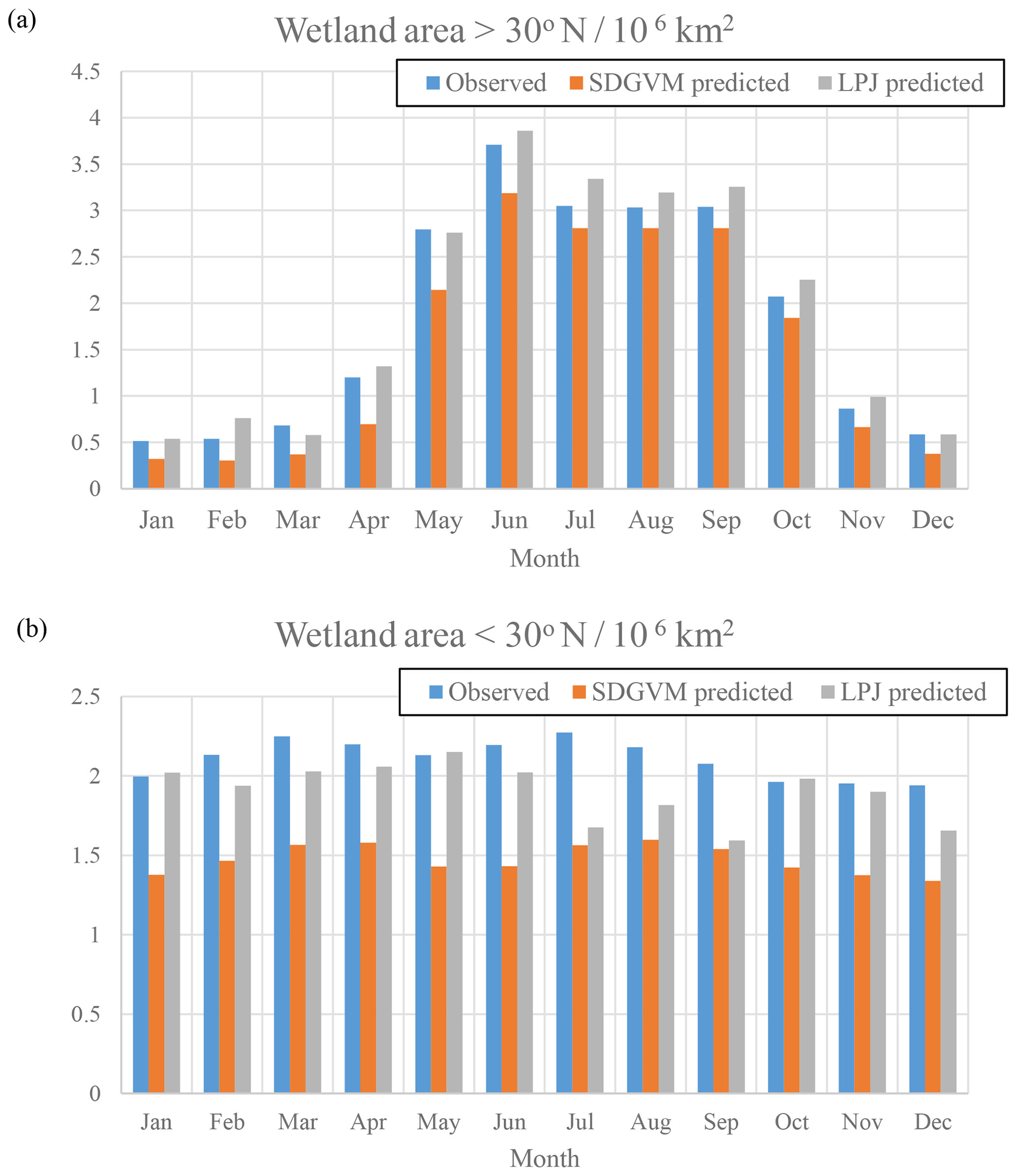
Figure 3 Monthly zonal variations in FW calculated for the mean 2000–2012 climate on a $\mathrm{2.5}{}^{\circ }\times \mathrm{3.75}$^∘ grid; (a) north of 30^∘ N and (b) south of 30^∘ N.

Table 2 Modern-day monthly mean FW area (10⁶ km²) for observed data interpolated to the 2.5^∘ × 3.75^∘ grid or calculated by vegetation model.

Figure 4 shows the monthly variation in wetland methane emissions for boreal and tropical areas, calculated using the observed or predicted FW, both vegetation model outputs and Eqs. (3) to (6). The annual methane emission totals are summarised in Table 3, along with other recent estimates from model intercomparisons. The annual and monthly zonal methane emissions are broadly similar for a given vegetation model regardless of whether the observed or predicted FW is used. SDGVM gives global emissions in line with the other modelling studies, whereas those from LPJ are somewhat lower. This is mainly due to differences in tropical emissions. SDGVM yields higher tropical emissions than LPJ but slightly lower emissions north of 30^∘ N. The main factors influencing the modelled methane emissions (other than FW) are, according to Eqs. (3) to (5), temperature (which is the same for both vegetation models), soil respiration (R_h) and gross primary productivity (GPP), the latter two differing between the two vegetation models. It appears that differences in R_h lead to the different zonal methane totals. South of 30^∘ N, SDGVM and LPJ model annual total R_h of 46 000 and 35 000 Tg C yr⁻¹, respectively, and, using the same observed FW, SDGVM and LPJ model annual methane emissions of 123 and 69 Tg CH₄ yr⁻¹, respectively. Therefore, in the tropics the differences in the predicted methane emissions seem to be due to differences in calculated R_h. North of 30^∘ N both DGVMs have similar R_h, 20 000 and 22 000 Tg C yr⁻¹, respectively, for SDGVM and LPJ, and similar values of methane emissions, 64 and 65 Tg CH₄ yr⁻¹, respectively.

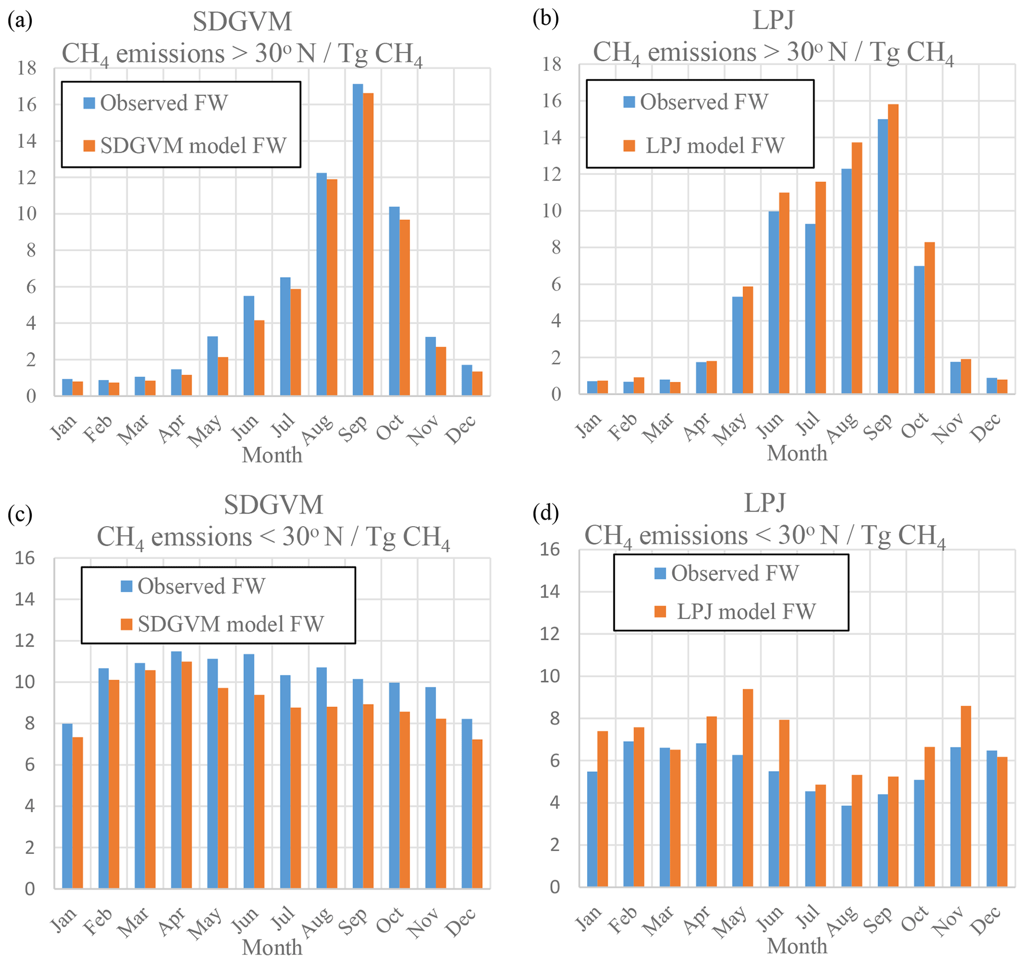
Figure 4 Monthly zonal variations in wetland CH₄ emissions (Tg CH₄) calculated from DGVM model data and observed or modelled FW for the mean 2000–2012 climate on a $\mathrm{2.5}{}^{\circ }\times \mathrm{3.75}$^∘ grid. (a) SDGVM north of 30^∘ N, (b) LPJ north of 30^∘ N, (c) SDGVM south of 30^∘ N and (d) LPJ south of 30^∘ N.

Table 3 Modern-day annual total wetland CH₄ emission (Tg CH₄ yr⁻¹), calculated by vegetation model using either observed FW data (interpolated to the 2.5^∘ × 3.75^∘ grid) or model predicted FW, compared with other modelling studies.

^a GCP-CH4 (Poulter et al., 2017) results are the mean of 11 different methane
emission models with the same observed wetland data as used to produce Fig. 1 here.
They are quoted as means over specific ranges of years: 2000–2006 = 184.0±21.1, 2007–2012 = 183.5±23.1 and 2012 = 185.7±23.2. As our results are for a single
mean 2000–2012 year we therefore only quote an approximate value from this source
for comparison. ^b WETCHIMP (Melton et al., 2013) results are the mean of
8 different models, 1993–2004, each of which used their own definition of wetland
extent rather than observed data.

We stress that this was a simple test for a nearest-neighbour approach for reasons outlined at the beginning of this section, and the satisfactory results obtained here merely indicate that this is an approach that has potential to be useful in predicting FW for a paleoclimate.

3.2 Early Eocene climate

In the previous section we have shown that a NN method can reproduce FW for a modern-day climate, justifying its application to the early Eocene climate described in Sect. 2.2. However, as noted at the end of Sect. 2.4, a NN method can be extended to KNN, whereby we predict FW based on some function of the FW of K nearest neighbours (noting that in Sect. 3.1, NN is simply 1NN, i.e. KNN with K=1). A 1NN algorithm that works well to predict modern-day FW may not work as well for a paleoclimate of many millions of years in the past. The reference data set we use, Sect. 2.1, is very similar to the modern-day test set, the latter's climate data are simply obtained by interpolating the former to a courser spatial grid. Therefore, we expected and observed a high correlation between modern-day FW predicted from the nearest neighbour in the reference data and the actual FW. The early Eocene test data has significant differences to the reference data since the climate of the early Eocene is obviously not the same as the modern day. Therefore, it will be harder for a nearest-neighbour-based method, searching a space described by climate and vegetation data, to find a nearest neighbour in the modern-day reference data with the correct early Eocene FW, whatever that may be. It may be that for a high FW early Eocene grid cell, the nearest neighbour happens to have quite low FW and vice versa. Figure 1 shows that FW can change from very high to almost zero over relatively small distances, for example in the Amazon basin, and therefore that sites with similar climate and vegetation can have very different FW. The greater the degree of difference between the early Eocene and the modern-day reference data sets, the more likely it is that the first nearest neighbour does not have the correct FW.

FW calculated for the early Eocene using the exact same 1NN method as used for the modern-day test set yields a value of global monthly mean wetland area of 4.07×10⁶ km² using SDGVM. This is around 33 % higher than that for the modern-day value, 3.00×10⁶ km², from Table 2. However, this includes a contribution of 1.53×10⁶ km² from areas south of 30^∘ S, which have an almost negligible contribution for the modern day, so the tropics and northern boreal regions actually have lower FW for the early Eocene. Given that the early Eocene was significantly warmer and wetter than the modern day (Carmicheal et al., 2017), we expect greater wetland area than the modern day. Beerling et al. (2011) reported global wetland area for an early Eocene climate using SDGVM; employing their method to our early Eocene climate, so as to eliminate differences arising from the specific HadCM3 model climate and spatial resolution, yields a global monthly mean FW area of 16.29×10⁶ km², 4 times higher than the value we would calculate from a 1NN method. Therefore, based on a comparison with both the modern-day studies and a previous Eocene study, it appears that a 1NN method may be unsuitable for a paleoclimate that is very different to our modern-day reference climate, and we consider KNN with higher values of K.

3.2.1 Maximum of K nearest-neighbour FW prediction

If indeed the 1NN results are too low then that implies that for some hypothetical high FW sites from the early Eocene, the first nearest neighbours in the reference data have very low FW. Therefore, if we consider higher values of K we may improve our estimate by predicting FW to be the maximum FW of K nearest neighbours (maxKNN) in the reference data. However, applying this approach will yield increasingly higher FW as K increases, requiring a data-constrained optimisation of K. Clearly there are no observations of Eocene wetland distributions with which to properly train any predictive algorithm, but we may utilise a suitable proxy for wetlands to try and obtain such a constraint. Here we use the distribution of coal deposits in the Eocene (Boucot et al., 2013), shown in Fig. 5 as such constraints. There are some limitations to this approach. Coal is formed in wetlands, but can also form in other settings such as lakes; and of course, these data sets do not document where wetlands were present but the sedimentary record is missing or has not been published. In the tropics, coal may not have formed in wetland environments due to a very high rate of carbon cycling and in northern latitudes subsequent glaciations could have eroded coal deposits away. Moreover, data will be sparse or non-existent for remote or inaccessible modern-day regions, such as under the Antarctic ice sheet. We also note that precise age and location, especially when comparing to low-resolution climate simulations, could cause disagreement for grid-by-grid comparisons. A final and critical complication is that FW is a number between 0 and 1, corresponding to the fraction of a site that is wetland, whereas the coal data are a binary measure: either a grid cell has or does not have a coal deposit within it. For all of these reasons, data–model comparisons must be done cautiously; nonetheless, these data are useful for identifying the most effective K value for reconstructing likely wetlands.

Figure 5 Locations of Eocene coal deposits plotted on our Eocene model land mask. The □ symbols indicate an Eocene coal deposit location (Boucot et al., 2013).

We defined two functions to assess how well a model FW matched the locations of Eocene coal deposits. Firstly, f1 is defined as the mean distance, in kilometres, of a coal deposit location to a grid cell with model FW predicted to be >0.2. The choice of 0.2 representing significant FW is arbitrary but the analysis was repeated with other values and the same conclusions were found. Secondly, f2 is defined as the mean FW of the grid cell closest to each coal deposit location, providing that site is within 2 grid points of that coal deposit location, to allow some leeway with regard to different projected locations of land masses in the early Eocene. Again the choice of a 2-pixel limit is arbitrary but the analysis was repeated with other limits and the same conclusions found.

Figure 6 shows the values of f1 and f2 for maxKNN predictions of FW with increasing K for both the SDGVM and LPJ early Eocene data sets, compared to a data set of coal deposit locations. As explained, since FW increases with K then, by extension, so does the likelihood of a site with a coal deposit in or close to it coinciding with a site of significant FW. Therefore, we do not seek to find the value of K that will give the lowest value of f1 and highest value of f2 as that would simply be K equal to the size of the entire reference data set. Instead, we try to find the lowest value of K that gives a “good” prediction for both f1 and f2. Although “good” is a subjective measure, we define it based on where increases in K result in marginal improvements in f1 and f2. For both vegetation models as K increases from 1 to 3 f1 decreases significantly and f2 increases significantly. For K>3 the decrease in f1 levels out and the increase in f2 also declines. Therefore, we conclude that based on comparison of predicted FW and locations of coal deposits, K=3 is a reasonable choice to make predictions for our early Eocene climate via a maxKNN algorithm.

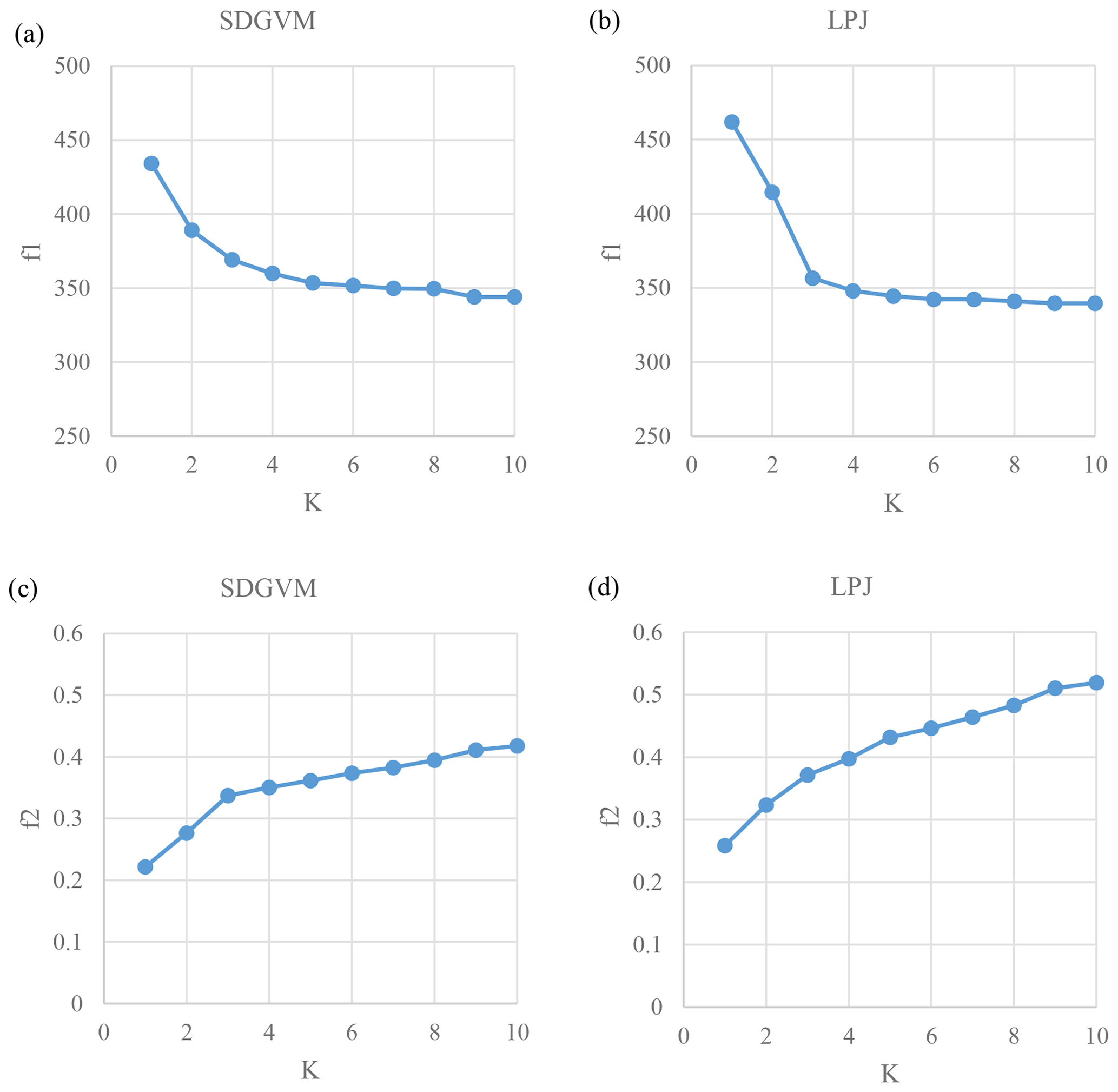
Figure 6 Variations of statistics for a match between Eocene maxKNN predicted high FW and coal locations (Boucot et al., 2013). The f1 is the mean distance of a coal location to site with FW>0.2 for model based on (a) SDGVM and (b) LPJ. The f2 is the mean FW of sites within 2 pixels of a coal location for model based on (c) SDGVM and (d) LPJ data.

3.2.2 FW predicted by max3NN

Figure 7 shows annual maximum FW (i.e. for each pixel the highest of the 12 monthly values) calculated by a max3NN model using SDGVM or LPJ vegetation data, as described above, with the locations of early Eocene coal deposits also shown. The annual maximum FW is shown here as FW might only need to be high at some point during the year to give rise to coal deposits. The areas of predicted high FW are much larger than for the modern day (Fig. 1); moreover, at this spatial resolution there are often abrupt changes from low to medium (yellow) to much higher (red) values leading to some isolated patches of high FW. The approach makes it difficult to interrogate specific factors that drive the increase in Eocene FW compared to today but given the wetter climate of the early Eocene, higher FW than the modern day is to be expected. The patchiness is partly a consequence of using annual maximum FW but also reflects the challenge of predicting a characteristic of a paleoenvironment based on modern-day reference data. Considering zonal total FW and seasonal average FW maps, i.e. averaging out some of the small-scale spatial and temporal variability, is likely a better approach for understanding ancient methane cycling and these are discussed later.

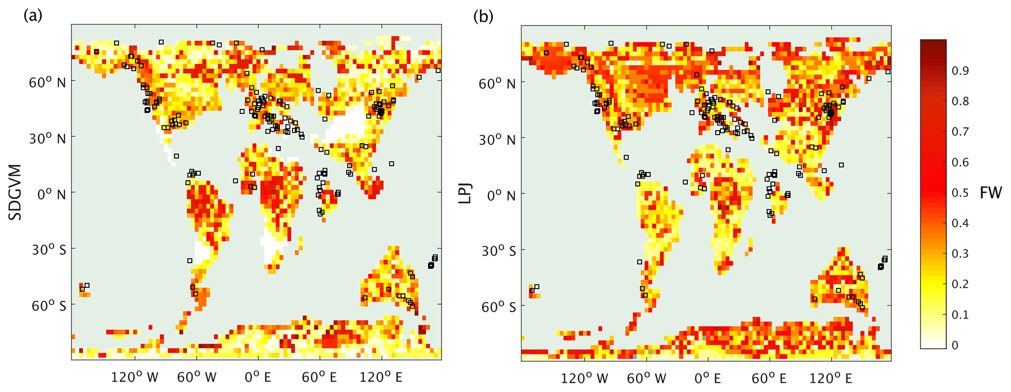
Figure 7 Annual maximum FW calculated by the max3NN method by (a) SDGVM and (b) LPJ for the Eocene climate, compared with coal deposit locations.

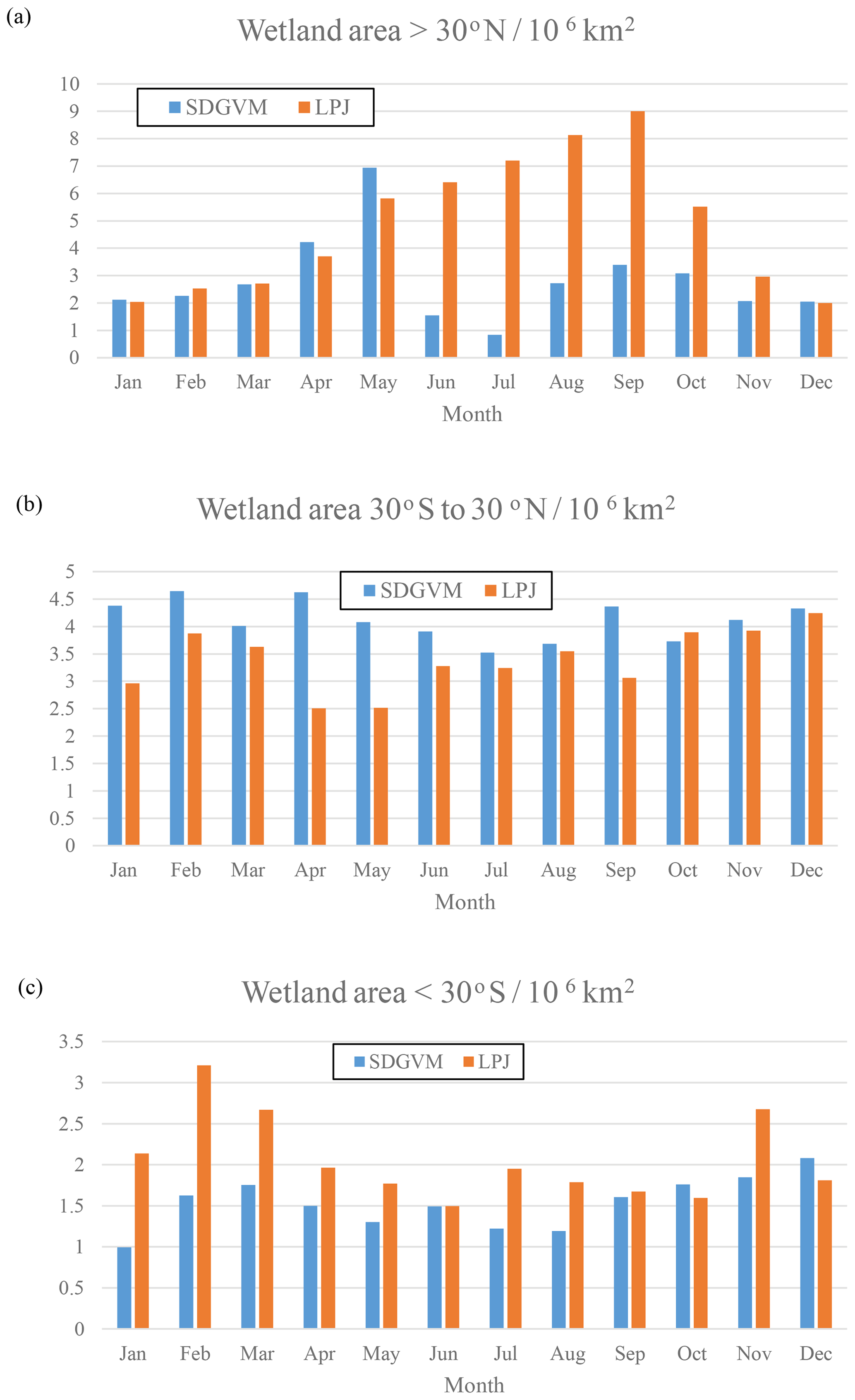
Figure 8 Monthly variations in total wetland area calculated for the Eocene climate by SDGVM and LPJ for (a) all areas north of 30^∘ N, (b) all areas between 30^∘ S and 30^∘ N and (c) all areas south of 30^∘ S.

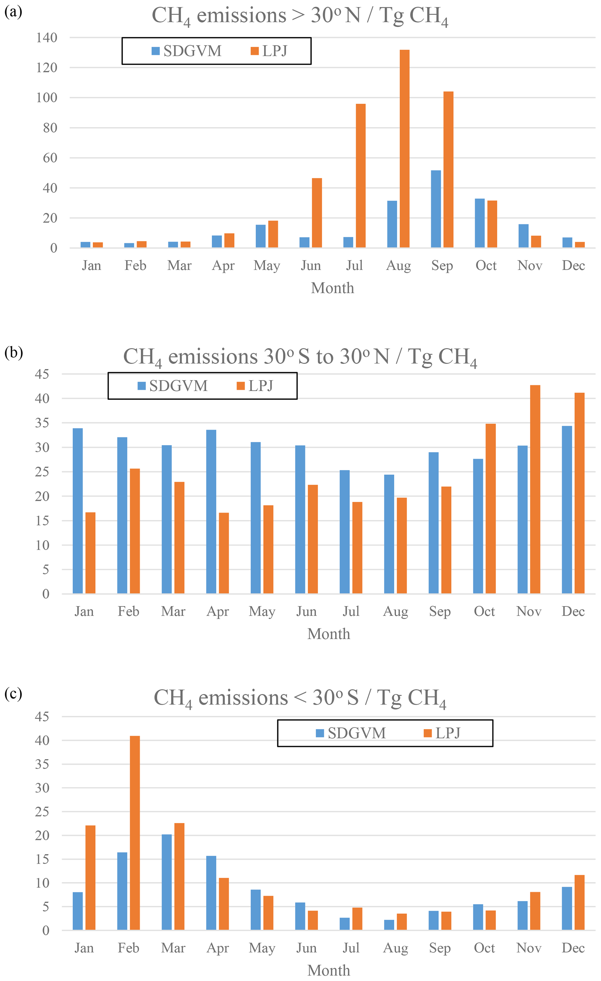
Figure 9 Monthly variations in wetland CH₄ emissions (Tg CH₄) calculated from predicted FW for the Eocene climate by SDGVM and LPJ, for (a) all areas north of 30^∘ N, (b) all areas between 30^∘ S and 30^∘ N and (c) all areas south of 30^∘ S.

The maps of predicted FW are quite different for the two vegetation models, but the greatest differences are in areas with very little or no coal deposits, e.g. the tropics, north-eastern North America and Antarctica, making it difficult to critically evaluate them against the data. However, the monthly variations given by the two vegetation models in total FW (Fig. 8) and methane emissions (Fig. 9) for the three latitudinal zones are reasonably similar with respect to seasonal variations in that both have their highest values in the late spring and summer months for zones north of 30^∘ N and south of 30^∘ S and no clear seasonal variation in the tropics. In the tropical zone, predictions of monthly FW area are similar in magnitude for the two vegetation models, with SDGVM usually predicting higher FW than LPJ. However, in the zone north of 30^∘ N LPJ predicts much higher FW than SDGVM throughout June to October with a peak in September, whereas SDGVM peaks in May. A similar but less striking pattern occurs for the zone south of 30^∘ S where again LPJ predicts higher summer FW area than SDGVM. These differences between the two vegetation models are also evident in maps of seasonal average predicted FW (Fig. 10). In June to August, SDGVM predicts very little wetland area in the Northern Hemisphere, whereas LPJ predicts moderate to high FW areas over much of the land north of around 50^∘ N. In December to February both models predict almost zero FW north of around 50^∘ N. In the tropics and the Southern Hemisphere, the two models predict similar amounts of wetland area, but with SDGVM predicting slightly higher FW overall between 30^∘ S and 30^∘ N and LPJ predicting slightly higher FW south of 30^∘ N.

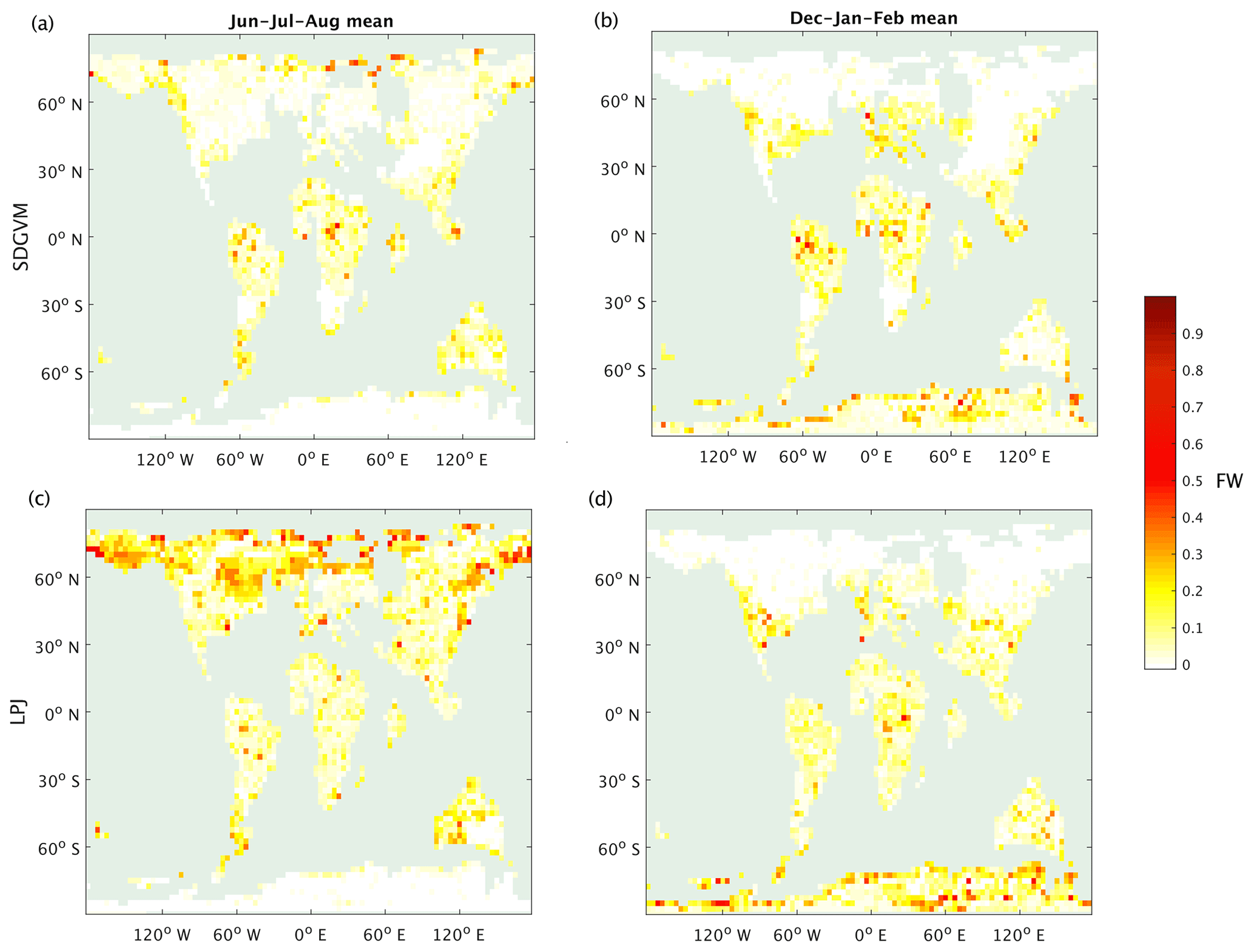
Figure 10 Seasonal mean FW predicted for the Eocene climate by SDGVM and LPJ using the max3NN (a) SDGVM June–July–August, (b) SDGVM December–January–February, (c) LPJ June–July–August and (d) LPJ December–January–February.

This differs from the modern-day distribution of wetlands (Fig. 1) and likely arises from a variety of method-dependent factors. First, the coarser resolution leads to a more patchy distribution, as is evident in the modern-day data in Figs. 1 and 2a and b at 0.5^∘ ×0.5^∘ and 2.5^∘ ×3.75^∘ spatial resolutions, respectively. This is particularly true for the tropics where wetlands do occur in small areas. Secondly, the nature of the nearest-neighbour algorithm relies on the principle that a grid cell in a paleoclimate with specific values of environmental variables will have the same FW as a grid cell in a modern-day reference data set with similar values for those environmental variables; however, other factors influence wetland fraction, such as the topography. Therefore, a nearest-neighbour method predicting FW for a paleoclimate from a modern-day reference data may well have errors for a given grid cell and month. These errors should reduce when averaged over latitudinal zones or seasonal averages.

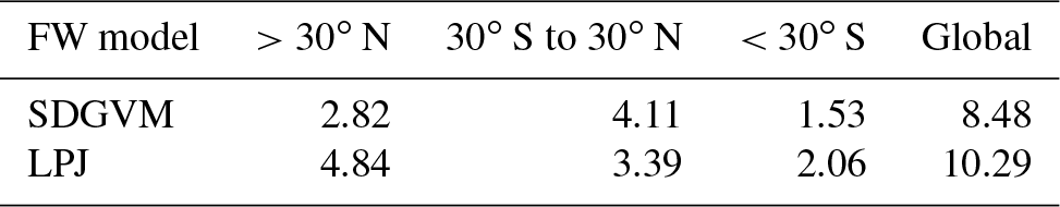
The differences between methane emissions from the two vegetation models likely arise from their respective impacts on soil water balance, via the magnitude of evapotranspiration (EVT) relative to precipitation (PRC). As the vegetation model, used to calculate EVT, and climate model, used to calculate PRC, are not dynamically coupled, PRC will be the same in all Eocene simulations, but EVT will vary; thus, vegetation models that yield elevated EVT in a given grid cell are more likely to yield a negative water balance (PRC − EVT) and low FW. Figure 11 shows the June to August mean PRC − EVT for SDGVM and LPJ, revealing that it is negative in most places north of 30^∘ N for SDGVM but is slightly positive or at least much closer to zero for LPJ. Therefore, SDGVM will generally predict lower FW by identifying modern-day nearest neighbours where PRC < EVT and unlikely to be wetland. The lack of extensive of coal deposits in the high northern latitudes, especially where the LPJ-based approach predicts wetlands, could indicate that the LPJ approach has over-predicted FW. However, we caution that this could be a data limitation issue and future work is required to interrogate the forecasts of these two methods. Regardless, both models yield broadly similar results on global and zonal terms (Table 4) indicating that the KNN algorithm could be a useful complementary approach for interrogating ancient wetland extent and methane emissions. Global monthly mean FW for the Eocene is 8.5×10⁶ and 10.3×10⁶ km² predicted by SDGVM and LPJ, respectively. Both of these values are larger than for the modern-day value of 3.0×10⁶ km², as we would have expected.

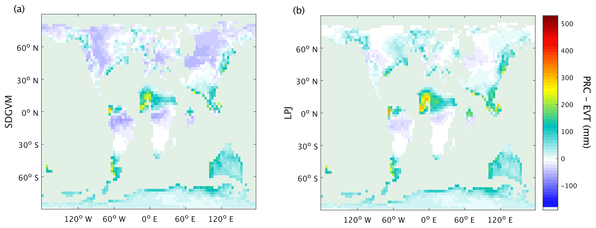
Figure 11 June–July–August mean precipitation minus evapotranspiration for the Eocene climate, using evapotranspiration from (a) SDGVM or (b) LPJ.

Table 4 Eocene monthly mean max3NN modelled FW area (10⁶ km²).

4 Conclusions

We have presented a nearest-neighbour method by which FW can be calculated at sites on the Earth's surface for an Eocene paleoclimate based on a set of environmental variables obtained from climate and vegetation models and a comparison of these to a modern-day reference data set. This has been used as an offline tool using data obtained from climate and vegetation models, rather than by embedding this within existing Earth system models, as the goal of this work was to explore and improve on methods of predicting FW for deep-time paleoclimates. The precise formulation of the nearest- neighbour approach was determined through comparison to locations of Eocene coal deposits and indicated that a max3NN method was best suited in this case. That should not be taken to imply that a max3NN would be the best in general; for another paleoclimate a similar analysis to that performed here would be required to determine the optimum implementation of KNN. It would therefore be of interest in future work to apply this methodology to other paleoclimates to see if similar results are obtained, perhaps using different environmental variables to those we have used to find nearest neighbours and perhaps other proxies for paleo-FW, should they become available. The predicted distributions of FW are much higher than those of today, as we would expect. We have assessed this using two different global vegetation models, and whilst these do yield some geographical differences in FW arising from different evapotranspiration estimates, they are broadly similar when considering zonal means. For both vegetation models, global monthly mean modelled FW area is less than, around half to two-thirds, that of Beerling et al. (2011), as are the values of the wetland methane emissions. However, our new method does not rely on the standard deviation of orography, a variable which is only known to a relatively coarse resolution for deep paleoclimates.