the Creative Commons Attribution 4.0 License.
the Creative Commons Attribution 4.0 License.
 | 22 Mar 2019
CORDEX-WRF v1.3: development of a module for the Weather Research and Forecasting (WRF) model to support the CORDEX community
Jan Polcher
Theodore M. Giannaros
Torge Lorenz
Josipa Milovac
Giannis Sofiadis
Eleni Katragkou
Sophie Bastin
The Coordinated Regional Climate Downscaling Experiment (CORDEX) is a scientific effort of the World Climate Research Program (WRCP) for the coordination of regional climate initiatives. In order to accept an experiment, CORDEX provides experiment guidelines, specifications of regional domains, and data access and archiving. CORDEX experiments are important to study climate at the regional scale, and at the same time, they also have a very prominent role in providing regional climate data of high quality. Data requirements are intended to cover all the possible needs of stakeholders and scientists working on climate change mitigation and adaptation policies in various scientific communities. The required data and diagnostics are grouped into different levels of frequency and priority, and some of them even have to be provided as statistics (minimum, maximum, mean) over different time periods. Most commonly, scientists need to post-process the raw output of regional climate models, since the latter was not originally designed to meet the specific CORDEX data requirements. This post-processing procedure includes the computation of diagnostics, statistics, and final homogenization of the data, which is often computationally costly and time-consuming. Therefore, the development of specialized software and/or code is required. The current paper presents the development of a specialized module (version 1.3) for the Weather Research and Forecasting (WRF) model capable of outputting the required CORDEX variables. Additional diagnostic variables not required by CORDEX, but of potential interest to the regional climate modeling community, are also included in the module. “Generic” definitions of variables are adopted in order to overcome the model and/or physics parameterization dependence of certain diagnostics and variables, thus facilitating a robust comparison among simulations. The module is computationally optimized, and the output is divided into different priority levels following CORDEX specifications (Core, Tier 1, and additional) by selecting pre-compilation flags. This implementation of the module does not add a significant extra cost when running the model; for example, the addition of the Core variables slows the model time step by less than a 5 %. The use of the module reduces the requirements of disk storage by about a 50 %. The module performs neither additional statistics over different periods of time nor homogenization of the output data.
- Article
(8735 KB) - Full-text XML
- BibTeX
- EndNote


Regional climate downscaling pursues the use of limited area models (LAMs) to perform climate studies and analysis (Giorgi and Mearns, 1991). It is based on the premise that, by using LAMs, modelers can simulate the climate over a region at higher resolution compared to global climate models (GCMs). Therefore, certain aspects of the climate system can be better represented due to the higher resolution and higher complexity of the parameterizations (inherent in LAMs) used to simulate physical processes, which cannot be explicitly resolved (e.g., shortwave and longwave radiation, turbulence, dynamics of water species). This methodology has been widely used for studying climate features, connections, and processes (Jaeger and Seneviratne, 2011; Knist et al., 2014; Kotlarski et al., 2017) and to produce climate data within the scope of continental, national, or regional climate change studies.
The Coordinated Regional Climate Downscaling Experiment (CORDEX; http://www.cordex.org/, last access: 18 March 2019) of the World Climate Research Program (WRCP) aims to organize different initiatives devoted to regional climate all around the globe following a similar experimental design (Giorgi et al., 2009; Giorgi and Gutowski, 2015). CORDEX, with the second phase currently under discussion, attempts to establish a series of criteria for dynamical downscaling experiments, which includes setting common domain specifications and horizontal resolutions in order to make sure that all the continental areas of the Earth are under study (e.g., in 2010 Africa was a priority and researchers worldwide volunteered to contribute with their own simulations). Furthermore, CORDEX sets a series of model configurations (e.g., GCM forcing, greenhouse gas (GHG) evolution) to ensure that model simulations are carried out under similar conditions and are therefore intercomparable. At the same time, CORDEX requires a list of variables necessary for the later use of model data in multi-model analysis and other climate-related research activities like climate change mitigation, adaptation, and stakeholder decision-making policies. In order to maximize and facilitate data access (mostly made available by the Earth System Grid Federation, ESGF; https://esgf.llnl.gov/, last access: 18 March 2019), these data also have to be provided following a series of homogenization criteria known as climate and forecast (CF) compliant (http://cfconventions.org/, last access: 18 March 2019), which come from the Coupled Model Intercomparison Project (CMIP) exercises. The list of variables required by CORDEX consists of standard model fields and some diagnostics in certain frequencies, as well as statistical aggregations such as minimum, maximum, or mean, for a given period. These variables are grouped into different priority levels (Core, Tier 1, and Tier 2), with Core being the mandatory list of variables (see Appendix A for more details).
The production of these datasets is not a simple task and usually represents a big issue for the modeling community. Regional climate experiments tend to produce large amounts of data, since scientists simulate long time periods at high resolutions. Modelers have to code software at least capable of (1) computing a series of diagnostics, (2) concatenating model output, (3) performing statistical temporal computations, and (4) producing data following CF-compliant (i.e., cmorization) criteria in NetCDF format (NetCDF stands for Network Common Data Form, a binary self-describing and machine-independent file format; https://www.unidata.ucar.edu/software/netcdf/, last access: 18 March 2019). Aside from being time-consuming due to complexity and process management, this codification also implies certain duplication of huge datasets and additional consumption of computational resources.
Several tools (e.g., NetCDF operators – NCOs, climate data operators – CDOs) exist to facilitate the manipulation of NetCDF files (extract, concatenate, average, join, etc.), and there are also other post-processing initiatives that have been made available, especially to the Weather Research and Forecasting (WRF; http://www.mmm.ucar.edu/wrf/users/, last access: 18 March 2019; Skamarock et al., 2008) community: WRF NetCDF Extract&Join (wrfncxnj; http://www.meteo.unican.es/wiki/cordexwrf/SoftwareTools/WrfncXnj, last access: 18 March 2019), wrfout_to_cf.ncl (http://foehn.colorado.edu/wrfout_to_cf/, last access: 18 March 2019), METtools (https://dtcenter.org/met/users/metoverview/index.php, last access: 18 March 2019), and Climate Model Output Rewriter (CMOR; https://cmor.llnl.gov/, last access: 18 March 2019).
WRF is a popular model for regional climate downscaling experiments. It is used worldwide in different CORDEX domains (Fu et al., 2005; Mearns et al., 2009; Nikulin et al., 2012; Domínguez et al., 2013; Vautard et al., 2013; Evans et al., 2014; Katragkou et al., 2015; Ruti et al., 2016). The model was initially designed for short-term simulations at high resolutions, but a series of modifications that have been introduced to the model code so far have enhanced its capabilities and made it appropriate for climate experiments (Fita et al., 2010). Since WRF does not directly provide most of the required variables for CORDEX and due to the complexity of the post-processing procedures, many existing WRF climate simulations are not publicly available to the community.
This new module comes to complement the modifications introduced in CLimate WRF (clWRF; http://www.meteo.unican.es/wiki/cordexwrf/SoftwareTools/ClWrf, last access: 18 March 2019; Fita et al., 2010). In clWRF climate statistical values (such as minimum, maximum, and mean values) of certain surface variables were introduced into the model. At the same time, the evolution of greenhouse gases (CO2, N2O, CH4, CFC-11, CFC-12) can be selected from an ASCII file instead of being hard-coded. Before these modifications, WRF users could only retrieve statistical values by post-processing the standard output of the model (at a certain frequency). With the clWRF modifications (incorporated into the WRF source code since version 3.5) statistical values are directly computed during model integration. This new CORDEX module proposes one step further by incorporating a series of new variables and diagnostics that are important for climate studies and WRF users can currently only obtain by post-processing the standard model output. At the same time, additional variables have been added into the WRF capabilities of output at pressure levels. In the current module version if the “adaptive time-step” option is enabled in WRF, some diagnostics related to time-step selection (e.g., precipitation, sunshine duration, etc.) will not be calculated properly because there is no proper adaptation.
We present a series of modifications to the model code and a new module (version 1.3) that will enable climate researchers using WRF to get almost all the CORDEX variables directly in the model output. With the use of this module, production of the data for regional climate purposes will become easier and faster. These modifications directly provide the required fields and variables (Core and almost all Tier 1; see Appendix A for more details) during model integration and aim to avoid the post-processing of the WRF output up to a certain level. However, in this version, they do not cover all the previously mentioned aspects of the task, such as computation of statistics and the cmorization of the data.
New variables and diagnostics will be provided at the user-selected output frequency. The user still needs to post-process the data in order to obtain the different statistics required by CORDEX at daily, monthly, and seasonal periods. The data cmorization can be defined as a series of processes that need to be applied to the model output in order to meet the standards provided under the CF guidelines (which follows the CMOR standard; https://pcmdi.github.io/cmor-site/, last access: 18 March 2019). These guidelines are designed to facilitate comparison between climate models, and they represent the standard for the Coupled Model Intercomparison Project (CMIP; https://cmip.llnl.gov/, last access: 18 March 2019). This standardization includes the file names, variable names, and metadata (units, standard name, and long name), specification of geographical projections, and time axis. In order to achieve a complete CF standardization of WRF output in complete agreement with the CF requirements, substantial changes to the WRF input/output (I/O) tools would be required. This would affect backward compatibility and it has been decided to pursue this in upcoming module updates. Therefore, the users of the CORDEX-WRF module will still need to perform part of the standardization. This includes joining and/or concatenating WRF files, making use of standard names and attributes of the variables and file names, and finally providing the right variable with the standard attributes to describe the time coordinate.
The module also aims to establish a series of homogenizations for certain diagnostics. These diagnostics can be computed following different methodologies, and consequently they may be model and/or even physical parameterization dependent. In order to avoid dependency on the model configuration (mainly sensitivity to the choice of the various available physical schemes), and to allow for a fair comparison between different simulations, a series of additional “generic” definitions of some diagnostics are presented when possible.
The modification of the WRF model code was initiated within the development of the regional climate simulation platform from the Institute Pierre Simone Laplace (IPSL) (https://sourcesup.renater.fr/wiki/morcemed/Home, last access: 18 March 2019) and the CORDEX Flagship Pilot Study (CORDEX-FPS), “Europe+Mediterranean; Convective phenomena at high resolution over Europe and the Mediterranean” (Coppola et al., 2018), in order to obtain the variables required for the CORDEX experiment (available at https://www.hymex.org/cordexfps-convection/wiki/doku.php?id=protocol, last access: 18 March 2019) and share the code among WRF users of the CORDEX-FPS experiment.
In this work the complete module is presented, its capabilities are demonstrated, and the results of several diagnostics are shown in order to illustrate the accuracy of the implementation. The initial section of the paper describes the modifications that have been introduced into the code, followed by a description of the variables required by CORDEX. The following section demonstrates the performance tests and gives a description of aspects that are currently missing, but will be added in the upcoming module versions. The paper finishes with a discussion and outlook.
Here we present the module and explain the modifications introduced. The
steps necessary in order to compile and use the module are provided as well.
For a complete and detailed description of the steps to follow, the reader is
referred to the Wiki page of the module:
http://wiki.cima.fcen.uba.ar/mediawiki/index.php/CDXWRF (last access:
18 March 2019). The most common README file provided with the module is
labeled README.cordex. The module has been implemented following the
standards of modularity, which facilitates the upgrading and introduction of
new variables to it.
2.1 WRF code main characteristics
First, we provide a short description of the WRF code characteristics. The
WRF model is written in Fortran 90. It is open access. It consists mainly of
two parts: WPS (WRF Preprocessing System) for the preparation of the initial
and boundary conditions and the model itself. The source of the code is
not fully provided. A pre-compilation process is carried out in order to
automatically write certain parts of the code according to a series of
ASCII files, and activation of certain parts of the code rely on
pre-compilation flags. With the pre-compilation flags users can determine
optional aspects of the model related to technical aspects of the compilation
and the use of certain components like the incorporation of the Community
Land Model version 4 (Oleson et al., 2010; Lawrence et al., 2011). Large parts of the code
that are automatically written are related to the input/output of the model.
There are a series of ASCII files provided in the Registry folder of
the model called registry. These files contain the characteristics of
the variables, mainly the name of the variable during execution, the rank and
dimensions of the variable, assigned output file, the name of the variable in the
output file, description of the variable, and units. The WRF model keeps all the
variables in a Fortran pointer-derived type (called grid). At the same
time, the WRF model setup is managed though the use of a Fortran
namelist
statement that reads the ASCII file called namelist.input, which has
different sections. WRF manages the output via different streams (usually up
to 23) with the standard output (wrfout+ files) being the number 0. The WRF
model integrates the atmosphere using η as a vertical variable (see
more detail in Skamarock et al., 2008) defined in Eq. (1) (where psurf is surface pressure,
ptop is pressure at top, p is hydrostatic
pressure, η=1 at the surface, and η=0 at the top of the atmosphere). WRF
uses three horizontal grids (two C grids staggered for winds) and two sets of vertical
coordinates (one staggered known as the “full” η levels, with the
un-staggered as the “half”-η levels).
For further technical details of the model, the reader is referred to WRF technical notes (http://www2.mmm.ucar.edu/wrf/users/docs/arw_v3.pdf, last access: 18 March 2019; Skamarock et al., 2008) and the user guide (http://www2.mmm.ucar.edu/wrf/users/docs/user_guide_v4/contents.html, last access: 18 March 2019).
2.2 Module implementation
The module is accompanied by a new registry file called
Registry/registry.cordex in which the variables and namelist parameters
related to the module are defined. The specific setup of the module is
managed in the WRF namelist in a new section called cordex. Aside from
the modifications of the code of the WRF model, the complete module currently
consists of two new modules:
-
phys/module_diag_cordex.F, the main module that manages the calls to the variables and performs the necessary accumulations for the calculations of statistical values (e.g., mean, maximum, minimum); and -
phys/module_diagvar_cordex.F, the module that contains the calculations of all the CORDEX variables separated into individual and independent 1-D Fortran subroutines.
A list of detailed information on the modifications introduced is given below.
-
The main call of the CORDEX module (
module_diag_cordex.F) has been added tophys/module_diagnostics_driver.F, which accounts for the management of diagnostics, and it has been modified in order to introduce the new pressure-interpolated variables. -
An input line to the
registry.cordexhas been added into the generalRegistry/Registry.EM_COMMON. -
The complementary pressure-interpolated variables have been introduced in the related registry
Registry/registry.diags. -
The complementary interpolated variables have been added in the module that performs the pressure interpolation (
phys/module_diag_pld.F). -
The initialization of the modified pressure interpolation has been added in
dyn_em/start_em.F. -
Modifications have been introduced in the
main/depend.commonandphys/Makefilefiles to get the module compiled. -
Specific changes for the inclusion of the water budget variables have been introduced in the
dyn_em/solve_em.Fmodule in order to get the advection terms of all water species. -
An ASCII file called
README.cordexwith the description and synthesized instructions for compilation and use is provided as well.
The model output is grouped into a single file (WRF's auxiliary history output
or stream no. 9) with a proposed file name (auxhist9_outname namelist
parameter in the &history section):
wrfcordex_d<domain>_<date>,
regulated with the standard WRF namelist parameters of output frequency
(auxhist9_interval), number of time steps per file
(frames_per_auxhist9), and format (io_form_auxhist9). Additional
CORDEX variables required at pressure levels have been included in the WRF
auxiliary output file number 23. These introduced CORDEX variables follow the
file setup via the currently existing namelist section called diags&.
2.3 Module use
Before the execution of WRF some preprocessing steps are necessary by the user that encompass the compilation of the code and its specific setup to be used during the execution time of the model. These are described in the following subsections.
Compilation
Pre-compilation flags need to be defined by the user, depending on his or her requirements. It is necessary to keep in mind that this is done due to efficiency constrains (see below in Sect. 6), although it is not a common procedure in the standard use of WRF. Usually WRF has almost all options available from a single compilation, switching options via the namelist.
Using the pre-compilation flag CORDEXDIAG, the CORDEX Core variables
will be produced. The Tier 1 and additional groups of variables can be
selected via the additional pre-compilation flag CDXWRF
(CDXWRF=1 for Tier 1 and CDXWRF=2 for Tier 2 and the
additionals). The reader is referred to Appendix B for more
details about the groups of CORDEX variables associated with each option.
The registry file (registry.cordex) has to be manually modified
accordingly to the selected pre-compilation flag (uncomment the associated
lines).
In order to adapt this derived type to the preselected compilation, it is also
necessary to modify the module's specific register file
(register.cordex) according to the chosen value given to the
additional pre-compilation CDXWRF flag (if used). This is done in a
way to control the size of a grid-derived type, which has a positive
impact on the model performance (see below). For a complete and detailed
description of these steps, the reader is referred to the Wiki page of the
module at
http://wiki.cima.fcen.uba.ar/mediawiki/index.php/CDXWRF.
According to the value given to the pre-compilation CDXWRF flag, a
different amount of variables is written out to the wrfcdx
output file (see more detail in Appendix B).
-
Using
CORDEXDIAGand withoutCDXWRF, all the CORDEX Core variables will be calculated. -
For CDXWRF=1, CORDEX Core+Tier 1 variables are clgvi, clhvi, zmla, and [cape/cin/zlfc/plfc/lidx]{min/max/mean}.
-
CDXWRF=2 is as CDXWRF=1, plus additional 3-D variables at the model η level (ua, va, ws, ta, press, zg, hur, hus), 2-D variables (tfog, fogvisblty{min/max/mean}, tds{min/max/mean}), and the water budget variables (wbacdiabh, wbacpw, wbacpw[c/r/s/i/g/h], wbacf, wbacf[c/r/s/i/g/h], wbacz, wbacz[c/r/s/i/g/h], wbacdiabh{l/m/h}, wbacpw{l/m/h}, wbacpw{l/m/h}[c/r/s/i/g/h], wbacf{l/m/h}, wbacf{l/m/h}[c/r/s/i/g/h], wbacz{l/m/h}, wbacz{l/m/h}[c/r/s/i/g/h]).
Moreover, the code also accounts for instantaneous CORDEX variables
provided as statistics (e.g., capemean, tdsmax, or all the
water budget variables). In order to get them, the user must follow certain
modifications of the code (and re-compilation) in
phys/module_diag_cordex.F, phys/module_diagnostics_driver.F,
and in the registry file registry.cordex.
2.4 Usage
Modifications of the module include two main sets of variables: (1) new variables and diagnostics and (2) additional variables interpolated at pressure levels. These two sets of variables are provided in two separated files. A new auxiliary output file in the ninth stream provides all the new variables and diagnostics required by CORDEX. Additional pressure-interpolated variables are included in the 23rd stream. Each of these files has to be set up in the namelist in the same way as with the standard WRF output files.
(Stackpole and Cooley, 1970)(Benjamin and Miller, 1990)(Yesad, 2015)Brasseur (2001)(Fita and Flaounas, 2018)(Nielsen-Gammon et al., 2008)(Manabe, 1969)(Milly, 1992)(Kunkel, 1984)(Smirnova et al., 2000)(Gultepe and Milbrandt, 2010)Table 1Setup parameters of the module_diag_cordex module for
the WRF namelist contained in the cordex section. See
the sections on variables for more details on the meaning of each methodology.
The methodologies preferred by CORDEX are marked by a, and the ones
without preference by CORDEX are marked by b; in these cases,
users can select the method according to their experience.

a Preferred by CORDEX. b No preference is specified by CORDEX.
A new section labeled cordex has to be added into the WRF's
namelist,
which allows users to choose or set up different options of the module. The
description of all the available options is provided in Table 1. In this section the user is required to choose the
implementation of the diagnostics to use, provide values to some
parameters for certain diagnostics, and activate or deactivate some of the
most computationally costly diagnostics. Default values for all the options
are provided in order to facilitate the use of the module.
This module has been tested under different high-performance computing (HPC) environments and compilations. It has been compiled with two compilers: GFortran and IFORT. Different parallelization paradigms include serial, distributed memory, and hybrid (distributed and shared), as well as the parallelized version of the NetCDF libraries. The tests have been performed mainly using two-nested domains with the second one being at convection-permitting resolution (no cumulus scheme activated). Under all these circumstances the module worked as expected.
Since the current version (v1.3) of the module, a text message with the version of the module has been printed in the standard output at the first time step of the model run in order to facilitate the detection of the module version that is being used.
CORDEX requires a series of mandatory variables grouped into the Core level and additional variables grouped into Tier 1 and Tier 2 levels. Furthermore, CORDEX also requires statistical values of specific variables, besides the instantaneous values. To meet the CORDEX specifications, regional climate models have to provide three kind of variables.
-
Instantaneous: values obtained at each model integration time step. An instantaneous value represents the field at the given instant of time over the given space encompassed within the grid point.
-
Statistics: values obtained as statistics of consecutive instantaneous values along a given period of time. The statistical computation could be minimum, maximum, mean, or accumulated values, as well as the flux. Thus, one statistical variable represents the temporal statistics of the field for a given period of time over the given space encompassed within the grid point. CORDEX guidelines also require different temporal aggregations: 3-hourly, daily, monthly, and seasonal.
-
Fixed: values that do not have an evolution in time. These fields are fixed over the simulation.
The WRF I/O file managing system provides an infrastructure for more than
20 different output files (called streams) at the same time. Each file is
independently managed, and therefore in the namelist a user has to set up
mainly two different options for each output stream: the frequency of an
output (frequency of writing out the variables to an output file in minutes,
e.g., 30, 60) and the number of frames per file (e.g., for 3-hourly frequency
eight frames per file will give a daily output). Variables can be written in
multiple streams (selected via the registry + files). During the
model integration, at the given time step corresponding to the defined output
frequency,
data will be written out to the output file. When a given file reaches the
selected amount of frames, it is closed and a new one is opened. The file
name usually follows the criteria of a given header name (e.g.,
wrfcdx for this module) and the current date of the simulation,
which is also set up in the namelist.
The CORDEX-WRF module is designed to provide the variables using the ninth stream, without reducing any of the capabilities of the model. Following this criterion, the module uses the same structure and components of the model designed to manage its I/O. This means that the statistical values are directly provided using the internal values between output frequencies. This ensures that, for example, a minimum value would be exactly the minimum value that the model simulated between output times. These variables are re-initialized after each stream output time (see Fig. 1). The WRF model is used in a myriad of applications and regions, and thus it was decided that statistical values will be provided at the selected frequency of the ninth stream. This gives more flexibility, allowing a user to get, e.g., high-frequency outputs. However, this will require the user to perform a post-processed aggregation of the output files in order to provide the required CORDEX statistics at the 3-hourly, daily, monthly, and/or seasonal periods. Users are strongly encouraged to use the output frequencies for the ninth stream, which are easy to combine in order to retrieve the required CORDEX statistics. It is necessary to highlight the fact that the statistics for a given period contained in the ninth stream correspond just to the instant in time of writing the field into the file (e.g., at a 3 h output frequency the value inside the file at [HH]+3:00:00 represents the statistics from [HH]:00:00 to [HH]+2:59:59). The WRF I/O does not allow us to produce static or fixed fields, and therefore this group of variables is not provided by the module.
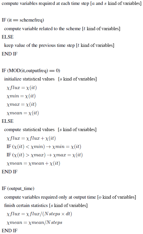
Figure 1Calculation of diagnostics according to the time step for each kind of variable (see tables in Appendix B).
3.1 Generic methodology
The list of variables requested by the CORDEX experiment (see the tables in Appendix B) is intended to be useful for the climate change mitigation, adaptation, and decision-making communities. Note that CORDEX-FPS might require other variables or require some of them at a different frequency of output in comparison to a standard CORDEX requested list of variables. Taking into account the performance of the model, variables are computed at specific frequencies: (1) at all time steps when a statistical value (accumulation and/or flux, minimum, maximum, and/or mean) of the variable is required, (2) at the given time step when a variable that is used for the diagnostic is updated following the configuration from the namelist (e.g., cloud-derived variables and the frequency of activation of the radiation scheme), and (3) instantaneous values that are computed only at the time step when the output is written out (see Fig. 1 for more details).
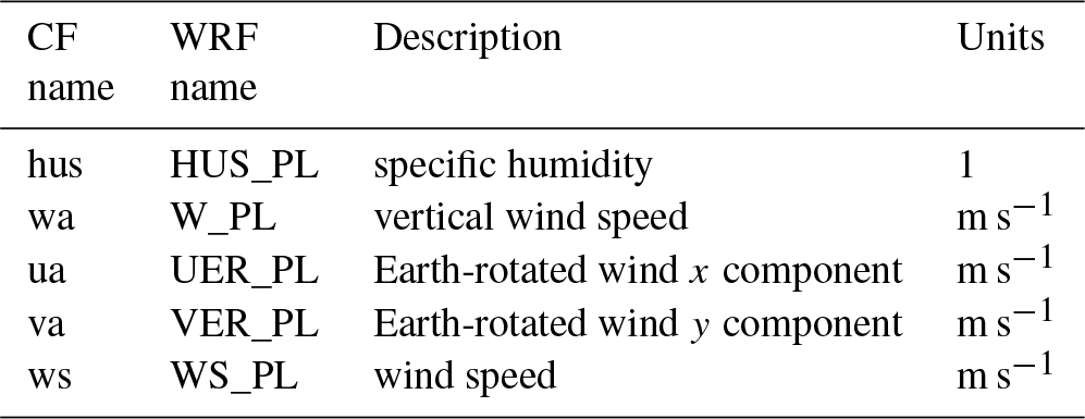
The list of added variables to the existing direct level pressure-interpolated output is provided
in Table 2 and gathered in
the 23rd auxiliary WRF output file with the standard name
wrfpres_d<domain>_<date> (in WRF's namelist notation). At the same
time, in order to avoid overloading the execution of WRF, the section of the
code with the pressure interpolation has also been modified. Now the
interpolation is only computed at the time step coincident with the output
frequency (also selected in the namelist along with the characteristics of
the pressure interpolation).
Table 2Description of CORDEX additional pressure-interpolated variables provided with the module.
The different statistical values are initialized (as shown in Fig. 1) at the first time step after output time. More details on how certain diagnostic variables have been integrated and implemented in WRF are provided in the following sections. Furthermore, a series of plots accompanying different definitions of the diagnostic variables are presented as well. The intention of these figures is to illustrate the consistency of the implemented diagnostics. These preliminary outcomes are not for validation purposes, but rather to show that the diagnostic variables have been correctly introduced. A complete analysis in order to find the most accurate methodology for the calculation of a certain diagnostic would require devoted climate simulations and enough observations to validate them. Such a validation is out of the scope of this study. We do select “more appropriate” options based on the experience within the scientific community or according to the CORDEX specifications. These options are set as the “default” options within the namelist.
One should be aware that certain diagnostics use variables for their calculation that might only be available when specific physical schemes are selected. When this happens, zero values are returned. This undesired outcome is, when possible, fixed by using a generic definition of the diagnostics.
3.2 Core variables
These are the basic variables required by CORDEX. Most of them are standard
fields and therefore tend to require simple calculations from the currently
available variables from the WRF model. These variables are obtained by
setting the pre-compilation flag CORDEXDIAG and will appear in two
different files: 3-D variables at pressure levels (the WRF model internally
interpolates them since it uses the η coordinate in the vertical) that will
appear in the output file with the 23rd stream (mainly called
wrfpress) and the 2-D variables in the module's output file
wrfcdx.
3.2.1 3-D at pressure levels
These are the additional variables that have been added into the WRF pressure-level integration module. Their values will be written in the 23rd output stream in addition to the ones currently available. All of them are instantaneous values.
hus: humidity
3-D atmospheric specific humidity (hus)1 and relative humidity (hur) are computed at the un-staggered model (half-)η levels. Specific humidity is simply obtained from the water vapor mixing ratio using Eq. (2) (named QVAPOR in WRF). Relative humidity can be obtained following the Clausius–Clapeyron formula and its approximation from the well-known August–Roche–Magnus formula for saturated water vapor pressure es (Eqs. 3, 4, and 5).
Here, tempC is temperature in degrees Celsius (∘C), presshPa is pressure (hPa), es is saturated water vapor pressure (hPa), and ws is the saturated mixing ratio (kg kg−1).
press: air pressure
The WRF model integrates the perturbation of the pressure field from a reference one. Thus, to obtain the full pressure at un-staggered model η levels, the user is required to combine two different fields as shown in Eq. (6):
where PB is WRF base pressure (Pa), and P is WRF perturbation pressure (Pa).
ta: air temperature
This variable stands for the 3-D atmospheric temperature on un-staggered model η levels. WRF model equations are based on the perturbation of potential temperature, and therefore a conversion to actual temperature is required, which is performed as indicated by Eq. (7):
where T is WRF 3-D temperature output (as potential temperature perturbation from the base value, which in WRF equals 300 K), and p0 is the pressure reference (100 000 Pa).
ua/va: Earth-rotated wind components
These variables stand for the 3-D atmospheric wind components following Earth coordinates on un-staggered model η levels. WRF model equations use the Arakawa C horizontally staggered grid with wind components following the grid direction. In order to get actual winds following Earth geographical coordinates, a transformation shown in Eq. (8) is required:
where Uunstg is un-staggered WRF eastward wind (m s−1, [1, dimx]), Vunstg is un-staggered WRF northward wind (m s−1, [1, dimy]), Ustg is x-staggered WRF eastward wind (m s−1, ), Vstg is y-staggered WRF northward wind (m s−1, ), cos a is the local cosine of map rotation (1), and sin a is the local sine of map rotation (1).
zg: geopotential height
As in the case of air pressure, the WRF model also integrates the perturbation of the geopotential field from a reference or base one. Thus, to obtain the full geopotential height on staggered model η levels, the user is required to combine the two WRF fields, and it is also de-staggered as shown in Eq. (9):
where PHB is WRF base geopotential height (m2 s−2), PH is WRF perturbation of the geopotential height (m2 s−2), zgstaggered is staggered geopotential height , and zg is un-staggered geopotential height .
3.2.2 Two-dimensional
Here we provide a list of the added two-dimensional CORDEX variables. Some of them are diagnosed as a combination of three-dimensional variables, some are required as instantaneous values, and others as statistics. The fact that the module provides 2-D variables online using 3-D fields shows one more key advantage of the module related to disk space. Thanks to these online calculations when using the module, a user no longer needs to store large amounts of 3-D data from the model in order to post-process them. This reduces the requirements of disk space by a factor of around 2.
pr, prc, prl, prsh, prsn: precipitation fluxes
The total precipitation flux (pr) is computed as the sum of all types of precipitation fields in the model accumulated along the ninth stream output frequency (9freq) divided by this period of time (9freq), as shown in Eq. (10):
where RAINCV is instantaneous precipitation from the cumulus scheme (kg m−2), RAINNCV is instantaneous precipitation from the microphysics scheme (kg m−2), RAINSHV is instantaneous precipitation from the shallow-cumulus scheme (kg m−2), Nsteps is the number of time steps, and δt is the time-step length (s) to achieve the ninth stream frequency output time ().
In this version, the computation of the accumulated values does not take into account configurations of the model with an adaptive time step. When an adaptive time step is used, we strongly discourage the use of these variables.
Each individual precipitation flux is also provided as follows.
Solid precipitation flux (prsn) only accounts for frozen precipitation.
Depending on the selected microphysics scheme chosen in the
namelist, this variable
might account for the precipitation of snow, graupel, and hail. It is
computed as shown in Eq. (12):
where prins is instantaneous total precipitation (kg m−2, previously obtained), and SR is the fraction of solid precipitation (%, variable provided by WRF).
Radiative flux
Surface upwelling shortwave radiation flux (rsus, W g m−2) and surface
upwelling longwave radiation flux (rlus, W g m−2) are understood as the
shortwave and longwave radiation from Earth's surface. They are directly
provided by the radiation schemes CAM (Community Atmosphere Model) and
RRTMG (Rapid Radiative Transfer Model) (sw_ra_scheme = 3,4) as
instantaneous variables swupb and slupb. When there is no use
of such schemes, it is recommended to use the generic definition instead
(rsusgen, rlusgen; see next section). Statistical retrieval for the
surface fluxes follows the same methodology as for the precipitation fluxes.
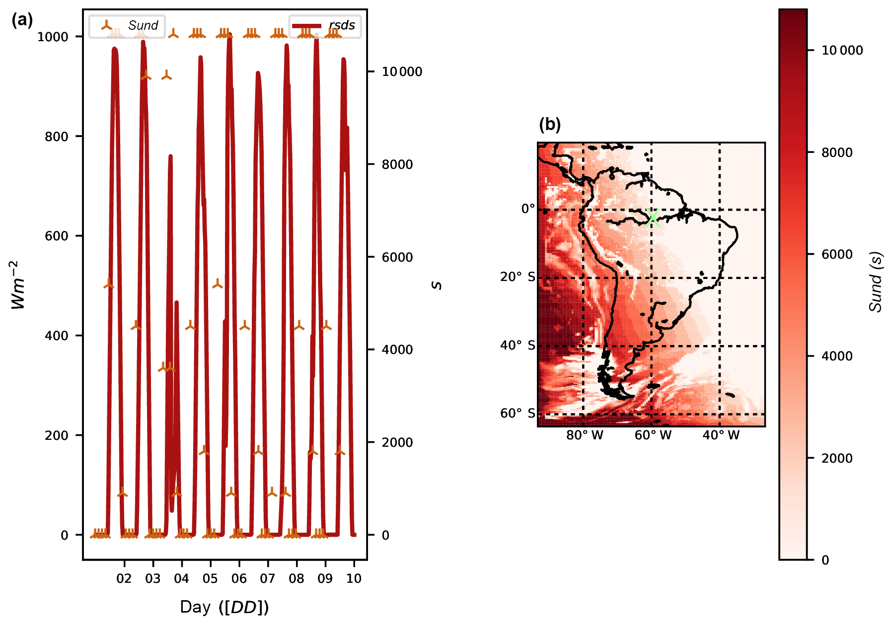
Figure 2Temporal evolution at 62∘4′38.00′′ S, 4∘58′55.51′′ W (a) of shortwave downward radiation (rsds, red line, left y axis) and sunshine duration for a 3-hourly 9freq (sund, stars, right y axis). (b) Sunshine length map on 9 December 2012 at 15:00 UTC. X denotes the position of the temporal evolution.
Outgoing radiative fluxes at the top of the atmosphere are also provided as “rsut” for mean top-of-atmosphere (TOA) outgoing shortwave radiation (in W g m−2) and “rlut” for longwave. However, there is no generic implementation of these variables.
sund: duration of sunshine
This variable accounts for the sum of the time for which the direct solar irradiance (downwelling shortwave radiation, rsds) exceeds 120 W m−2 (WMO, 2010a); it is implemented following Eq. (13) and provided in seconds. In order to provide an example of the correct implementation of this diagnostic, preliminary results are shown in Fig. 2. The figure shows the “sund” values and compares them with the incoming solar radiation. It is shown how the “sund” values vary accordingly to the moment of the day with zero values during night (panel a) or persistent totally cloud-covered regions (map in panel b):
where SWDOWN is downward shortwave radiation (W m−2), and δt is time-step length (s).
tauuv: surface downward wind stress
Instantaneous surface downward wind stress at 10 m accounts for the force that winds exert on the Earth's surface. It is implemented following Eq. (14):
where CD is the drag coefficient (1), uas is Earth-rotated
eastward 10 m surface wind (m s−1), and vas is Earth-rotated northward
10 m surface wind (m s−1). The drag coefficient is nonzero only for
certain options of the surface-layer physics (sf_sfclay_physics
parameter in the namelist): 1 (MM5-similarity) or 5 (MYNN
surface layer). A generic formulation has been introduced when these schemes
are not used.
psl: sea level pressure
This variable accounts for the instantaneous pressure extrapolated to the sea
level. It represents the value of the pressure without the presence of
orography. In order to provide a framework ready to implement different
methodologies, three different methods have already been implemented. The
choice of method can be controlled by a new namelist.input
parameter labeled psl_diag in the cordex section. The implemented
methods are the following:
-
the hydrostatic Shuell method (Stackpole and Cooley, 1970) already implemented in the module
phys/module_diag_afwa.F, assuming a constant lapse rate of −6.5 K km−1, selected when in the WRF CORDEX namelist section setting the parameter[psl_diag = 1]; -
the ptarget method (Benjamin and Miller, 1990) that uses smoothed surface pressure and a target upper-level pressure, already implemented in the WRF post-processing tool called
p_interp.F90[psl_diag = 2]; and -
the ECMWF method (Yesad, 2015) taken from the Laboratoire de Météorologie Dynamique GCM (LMDZ; Hourdin et al., 2006) from the module
pppmer.F90, following the methodology by Mats Hamrud and Philippe Courtier from ECMWF[psl_diag = 3].

Figure 3Sea level pressure estimates following the hydrostatic Shuell method at a given time step (pslshuell, a), ptarget (pslptarget, b), and ECMWF (pslecmwf, c). Bottom panels show differences among methods pslshuell − pslptarget (d), pslshuell − pslecmwf (e), and pslptarget − pslecmwf (f).
According to the CORDEX specifications, the default method is the ECMWF
method. When choosing the ptarget method (psl_diag = 2),
the degree of smoothing of the surface using the surrounding nine-point
average can also be chosen by selecting a number of smoothing passes
(psmooth, default 5), and the upper pressure that has to be
used as the target (ptarget, default 700 hPa).
Figure 3 shows the different outcomes when applying each method. There are some problems with the ptarget method in both psl estimates (mountain ranges can still be inferred) and borders for each parallel process (lines in figures showing differences among methods) when the spatial smoothing is applied. Lines showing the limits of the parallel processes appear because one cannot obtain the proper values from outside the correspondent tile of the domain associated with each individual parallel process.
Cloud-derived variables
Four cloud-derived variables are required by CORDEX: the total cloudiness (clt) and the cloudiness for each grid point at three different vertical layers aboveground (low: p≥680 hPa, labeled cll; medium: hPa, clm; high: p<400 hPa, clh). These cloud diagnostics are provided as mean values.
The module computes these variables taking the cloud fraction of a given grid
cell and level as input. The cloud fraction in WRF is computed by the
radiative scheme, and it is called at a frequency given by the radt
parameter in the WRF namelist. Due to the large computational cost of the
radiative scheme, radt is usually larger than the time step of the
simulation. This determines when cloud fraction is also actualized to meet
the evolved atmospheric conditions. Cloud fractions can be computed in the
model using different methodologies. It would be possible to make available
these methodologies as another choice in the namelist section and then
compute the cloud fraction at each time step. However, in order to be
consistent with the radiative cloud effects that the simulation is
experiencing, this method was discarded. Thus, the cloud values provided by
the module follow the same frequency of refreshing rate as the one set for
radiation in the namelist level (radt value).
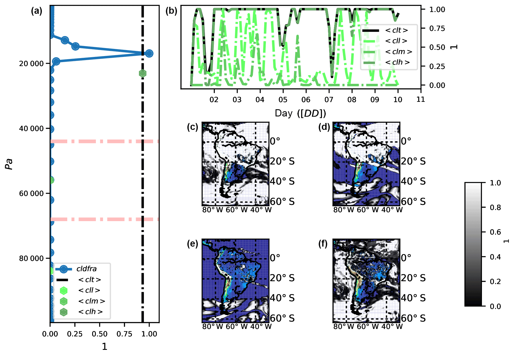
Figure 4Vertical distribution of cloud fraction and the different cloud layers on 9 December 2012 at 15:00 UTC at 62∘4′38.00′′ S, 4∘58′55.51′′ W (a): cloud fraction (cldfra, full circles with line in blue), mean total cloud fraction (clt, vertical dashed line), mean low-level cloud fraction (cll p≥680 hPa, dark green hexagon), mean mid-level cloud fraction (clm hPa, green hexagon), and mean high-level cloud fraction (clh p<440 hPa, clear green hexagon). Temporal evolution of cloud layers at the given point (b). Map of clt with colored topography beneath to show cloud extent (c); map of clh (d), map of clm (e), and map of cll (f).
The most common implementation of clt found in other models (in particular
most GCMs) assumes “random overlapping”. Random overlapping
assumes that adjacent cloud layers are from the same system and are hence
overlapped at a maximum (Geleyn and Hollingsworth, 1979). In the module, the methodology from
the GCM LMDZ was implemented. In this GCM, calculation of the total
cloudiness and different layers' cloudiness is done inside the subroutine
newmicro.f90. The method basically consists of a product of the
consecutive nonzero values of cloud fraction as shown in Eq. (15):
where CLDFRAC is the cloud fraction (1) at each vertical level, zclear is the clear-sky value (1), zcloud is the cloud–sky value (1), and ZEPSEC is a value for a very tiny number. The same methodology as in Eq. (15) is applied for the diagnostic of clh, clm, and cll but splitting by corresponding pressure layers. Figure 4 illustrates the result of the implementation and compares the results with the actual values of the cloud fraction (panels a and b), as well as the different cloud distributions (panels c to f).
Wind-derived variables
CORDEX requires two wind-derived diagnostics: the daily maximum near-surface wind speed of gusts (wsgsmax) and the daily maximum wind speed of gusts at 100 m aboveground (wsgsmax100). These variables cannot be retrieved by post-processing the standard output since they require the combination of different variables (some of them are not available from the model output) and have to be produced as a maximum value. The module provides different ways to compute them under certain limitations.
wsgsmax: maximum near-surface wind speed of gusts. The wind gust
accounts for the wind from upper levels that is projected to the surface due
to instability within the planetary boundary layer. In the current version of
the module two complementary methods of diagnosing the variable have been
implemented (resultant winds are Earth-rotated). The choice between the two
methods is done by the parameter labeled wsgs_diag (in
cordex
section), with the default value set to 1. The implemented methods
are the following (in italics).
-
The Brasseur method [
wsgs_diag = 1]. This is an implementation of wind gust considering turbulent kinetic energy (TKE) estimates and stability defined by virtual temperature (θv) as indicated in Eq. (16) following Brasseur (2001). Implementation is adapted from a version already introduced in the CLimate WRF (clWRF; http://www.meteo.unican.es/wiki/cordexwrf/SoftwareTools/ClWrf; Fita et al., 2010):where TKE is turbulent kinetic energy (m2 s−2), and θv is virtual potential temperature (K). zp is the height of the considered parcel (m, maximum height that satisfies Eq. 16), and Δθv(z) is the variation in θv over a given layer (K m−1).
-
The AFWA method [
wsgs_diag = 2]. This is an implementation adopted from the WRF modulemodule_diag_afwa.Fthat calculates the wind gust that only occurs as a blending of upper-level winds, zagl (around 1 km aboveground; zagl(k1000)≥1000 m; see Eq. 17), when precipitation intensity per hour is above a given maximum value (prate mm h−1):where va is air wind (m s−1), zagl is height aboveground (m), and k1000 is the vertical level at which zagl is equal to or above 1000 m; is the hourly precipitation rate (mm h−1), and vablend is blended wind (m s−1).
Figure 5Near-surface wind-gust estimates on 9 December 2012 at 15:00 UTC. 3 h maximum total wind-gust strength (wsgsmaxtot, a), percentage of wsgsmaxtot following the Brasseur method (wsgsmaxb01, b), percentage following the AFWA heavy precipitation implementation (wsgsmaxhp, c), percentage of time steps for which a grid point got a total wind gust (d), percentage of time steps for which a grid point got wsgsmaxb01 (e), and percentage due to wsgsmaxhp (f).
The two methods provide wind-gust estimation (WGE) from two different perspectives: mechanic and convective. In order to take into account both perspectives, additional variables are used: totwsgsmax (total maximum wind-gust speed at the surface), totugsmax (total maximum wind-gust eastward speed at the surface), totvgsmax (total maximum wind-gust northward speed at the surface), and totwsgspercen (percentage of time steps along 9freq in which a grid point got a wind gust in %). Figure 5 shows the outcomes when applying each method. It is shown how wind gust is mainly originated by turbulence, with a minor impact of heavy precipitation events at the depicted time. Furthermore, in the bottom panels it is shown how wind gusts are highly frequent above the sea in comparison to the low frequency above continental flat areas (the Andes mountain range exhibits a high occurrence of wind gust).
wsgsmax100: daily maximum wind speed of gusts at 100 m. The
calculation of wind gusts at 100 m should follow a similar implementation as
used for calculating the wsgsmax, but at 100 m. An extrapolation of
such turbulent phenomena would require a completely new set of equations that
have not been established yet. However, it could be considered as a first
approach to take the same wind gust as the one at the surface (when it is
deflected from above 100 m). The assumption would be that the wind gust at
100 m corresponds to the deflected wind on its “way” to the surface.
Instead, as a way to complement this, the estimation of maximum wind speed at
100 m is provided. Provided wind components are also Earth-rotated. Three
different methods have been implemented: two following assumed vertical wind
profiles (after the PhD thesis of Jourdier, 2015) and a third one
following Monin–Obukhov theory to estimate the wind components aboveground.
These three methods are chosen by the namelist parameter labeled
wsz100_diag. Its default value is 1. The implemented
methods are as follows.
-
[wsz100_diag = 1], following the power-law wind vertical distribution as depicted in Eq. (18) using the upper-level atmospheric wind speed below () and above () the height aboveground of 100 m (zagl). -
[wsz100_diag = 2], following logarithmic-law wind vertical distribution, as depicted in Eq. (19), using upper-level atmospheric wind speed below () and above () the height aboveground of 100 m (zagl). -
[wsz100_diag = 3], following Monin–Obukhov theory. The user should keep in mind that this method is not useful for heights larger than a few decimeters (z>80 m). The wind at a given height is extrapolated following turbulent mechanisms. As shown in Eq. (20), the surface wind speed is used as a surrogate to estimate the 100 m wind direction (, without considering Eckman pumping or other effects on wind direction). In this implementation u∗ in similarity theory is taken because the WRF estimates UST and Monin–Obukhov length (ℒO) as the WRF values for RMOL and roughness length (z0), with the WRF thermal time-varying roughness length ZNT:where wss100 is wind speed at 100 m (m s−1), ΨM is the stability function after Businger et al. (1971), UST is u∗ in similarity theory (m s−1), z0 is the roughness length (m), U10 and V10 represent 10 m wind speed (m s−1), θ10 is the 10 m wind speed direction (rad), ua100 is the 100 m eastward wind speed (m s−1), and va100 is the 100 m northward wind speed (m s−1). Note the absence of correction in wind direction due to Ekman pumping or other turbulence effects.

Figure 6100 m wind estimates. Comparison between upper-level winds and estimation on 9 December 2012 at 15:00 UTC at 62∘4′38.00′′ S, 4∘58′55.51′′ W. (a) 3 h maximum eastward wind (red) at 100 m by power law (uzmaxpl, star marker), Monin–Obukhov theory (uzmaxmo, cross), by logarithmic law (uzmaxll, sum), 10 m wind value (uas, filled triangle), and upper-level winds (ua, filled circles with line), also for the northward component (green). Temporal evolution of wind speed (b) with all approximations and upper-level winds at the closest vertical level at 100 m (on a log y scale, on average). Maps of three estimations: power law (c), Monin–Obukhov (d), and logarithmic law (e), with the blue cross showing the point of previous figures. Vertical distribution of winds at the given point in a wind-rose-like representation (f).
The user can also select the height at which the estimation is computed
throughout the namelist parameter z100m_wind (100 m as the default
value). Figure 6 shows different preliminary results using
the three different approximations. It is illustrated (panel a) how
wind gusts are larger than the 10 m diagnostic winds, and the difference
is also larger when using the Monin–Obukhov method compared to the two other methods.
Certain problems (too-small Monin–Obukhov length) are recognized when
applying Monin–Obukhov for extrapolating wind at 100 m, which is shown in
panel (b), where wind gusts appear to be as strong as 80 m s−1. Therefore,
users are advised to adopt this method with care.
Table 3Mixing ratio associated with column-integrated variables.
Vertically integrated variables
The instantaneous vertically integrated amount of water vapor (prw), liquid
condensed water species (clwvi), ice species (clivi), graupel (clgvi), and hail
(clhvi) are the vertically integrated amounts of each species along the
vertical column (density weighted) over each grid point. They are provided
using the same implementation as those in the p_interp.F WRF tool for
vertical interpolation. The general equation following WRF standard variables
is
where clvivar is the column vertically integrated variable's CF-compliant name (prw, clwvi, clivi, clgvi, or clhvi), MU is the perturbation dry air mass in the column (Pa), MUB is the base-state dry air mass in the column (Pa), g is gravity (m s−2), e_vert represents the total number of vertical levels, WRFVAR is the water species mixing ratio at each sigma level (kg kg−1), and DNW is the difference between two consecutive full η levels (–). Table 3 indicates the WRFVAR names associated with the clvivar names.
Figure 7On 9 December 2012 at 15:00 UTC at 62∘4′38.00′′ S, 4∘58′55.51′′ W: (a) water path (prw, vertical straight line in millimeters top x axis), vertical profile of water vapor (qv, line with full circles in kg kg−1 bottom x axis), and water path at each level (line with crosses). Map of water path (b) on 9 December 2012 at 15:00 UTC; red cross shows where the vertical accumulation is retrieved.
Note that clgvi and clhvi are part of the Tier 1 level and are only
accessible if the pre-compilation variable CDXWRF is set to 1. See Sect. 2.3 for more detail. In order to provide an example of the correct
computation of the diagnostics, results at a given grid point are shown in
Fig. 7. It is shown that the total precipitable water (prw)
correctly corresponds to the density-weighted vertical integration of the
water content along the column of air.
evspsblpot: potential evapotranspiration
This variable represents the evaporative demand of the atmosphere. It is
computed following the standard method already implemented in most GCMs. One
of the first proposed methods was provided by Manabe (1969). Some
corrections have been proposed to the initial methodology in order to
overcome its deficiencies (see, e.g., Barella-Ortiz et al., 2013, for an
intercomparison among different methods). It is provided as an averaged flux.
Calculation of the potential evapotranspiration can be activated with the
namelist input parameter potevap_diag (number 2 is the default
option).
-
The bulk method
[potevap_diag = 1]corresponds to the original one proposed in Manabe (1969). It basically consists of a difference between a supposed saturated air at the surface temperature and the humidity of the atmosphere as depicted in Eq. (22):where ws(ts) is saturated air at ts (kg kg−1), qc is the surface drag coefficient (m s−1), TSK is surface temperature (K), ws(ts) is saturated air by surface temperature (kg kg−1) based on the August–Roche–Magnus approximation, U10,V10 represent the 10 m wind components (m s−1), QVAPOR is the 3-D water vapor mixing ratio (kg kg−1), and CD is the drag coefficient (–, only available from MM5 similarity and MYNN surface-layer schemes; otherwise, it is zero).
-
The Milly92 method
[potevap_diag = 2]makes a correction of the bulk diagnostic by introducing a Milly correction parameter ξ, which accounts for other atmosphere-related phenomena (Milly, 1992). It is explained in Eq. (23), and its implementation is similar to the one present in the ORCHIDEE model (Organising Carbon and Hydrology in Dynamic Ecosystems; http://orchidee.ipsl.fr/, last access: 18 March 2019; de Rosnay et al., 2002). The implementation is retrieved from the modulesrc_sechiba/enerbil.f90:where β is the moisture availability function, sfcevap is QFX surface evaporation (kg m−2 s−1) from QFX, which is the surface moisture flux (kg m−2 s−1), L is the latent heat of vaporization, EMISS is emissivity (1), CtBoltzmann is the Stefan–Boltzmann constant, Cp is the specific heat of air, and ∂Tws(T) is the derivative of saturated air at the temperature of the first atmospheric layer (kg kg−1) using numerical first-order approximation.
Figure 8Evolution (a, in y log scale) of potential evapotranspiration by bulk (yellow) and Milly92 (blue) generic (dashed lines) methods at 4∘58′55.524′′ S, 62∘4′37.92′′ W (blue cross in panel b). On 18 November 2015 15:00 UTC, potential evapotranspiration following Milly correction (b), differences between the two methods (c, evspblpotMilly92−evspblpotbulk), differences between the two generic methods (d, ), differences between the Milly method and its generic counterpart (e, ), and differences between the bulk method and its generic counterpart (f, ).
See Fig. 8 for an example of the differences between the two implementations. It shows how important the correction introduced by Milly is and its strong effect on the diurnal cycle. Basically, the correction permits potential evapotranspiration during nighttime and reduces its strength at noon (18:00 UTC corresponds to 12:00 local time). There is a generic diagnostic to overcome boundary layer scheme dependency in the calculation of the drag coefficient (see the sections below on generic variables).
3.3 Generic variables
Some of the diagnostics required by CORDEX depend on the approximations, equations, methodologies, and observations used to compute them. This makes model intercomparison very difficult, since values might differ from one implementation to another. In order to overcome this problem, a series of variables is also provided in a generic form (when possible), meaning that they are obtained directly from standard variables. Thus, these generic forms of the diagnostics become “independent” of the model's implementation.
cdgen: generic surface drag coefficient
Computation of the instantaneous drag coefficient at the surface depends on the selected surface scheme. In order to avoid this scheme dependency, a generic calculation of the coefficient has been introduced as in Eq. (24) following Garratt (1992):
with UST u∗ being friction velocity from the similarity theory (m s−1), and the 10 m wind speed (m s−1).
tauuvgen: generic surface downward wind stress
Generic surface downward wind stress at 10 m is calculated following Eq. (25), which uses the generic diagnostics of the drag coefficient:
where is the generic drag coefficient (–, see Eq. 24), uas is the Earth-rotated eastward 10 m wind component, and vas is the Earth-rotated northward 10 m wind component.
rsusgen: surface upwelling shortwave radiation
Surface upwelling shortwave radiation is the shortwave radiation directed from the surface. It is calculated in a generic way as the reflected shortwave radiation depending on the surface albedo as shown in Eq. (26):
where ALBEDO is albedo (1), and SWDOWN is downward shortwave radiation at the surface (W m−2).
rlusgen: surface upwelling longwave radiation
Surface upwelling longwave radiation is the longwave radiation coming from the surface. It is calculated in a generic way as the longwave radiation from a black body due to surface temperature following the Stefan–Boltzmann law as given in Eq. (27):
where CtBoltzmann is the Stefan–Boltzmann constant ( W m−2 K−4), EMISS is surface emissivity (1), and TSK is skin temperature (K).
evspsblpotgen: generic potential evapotranspiration
This variable corresponds to the generic definition of potential evapotranspiration (evspsblpot). The same two methodologies as in the regular diagnostic have been implemented. The only difference is that, in this case, the generic estimation of the drag coefficient “cdgen” is used (see Eq. 24) instead of the one given by the model.
3.4 Tier 1 variables
These diagnostics are required by CORDEX, but they are not mandatory. They
have also been included as a way to fulfill all the CORDEX requirements.
These variables require the setting of the pre-compilation flag
CDXWRF
to 1 and performing some complementary modifications in the module's registry
file registry.cordex. See Sect. 2.3 for more details.
zmlagen: generic boundary layer height
Instantaneous planetary boundary layer (PBL) height is a clear example of model dependence and even scheme dependence of how a diagnostic is computed. Each PBL scheme has its own assumptions, and “zmla” is computed in a scheme-dependent specific way.
In order to overcome the model and/or scheme dependence, we implemented a generic formulation for calculating the PBL height as was done in García-Díez et al. (2013) after Nielsen-Gammon et al. (2008). The method consists of defining the height of the PBL as the first level in the mixed layer (ML) where potential temperature exceeds the minimum potential ML temperature by more than 1.5 K. It has been implemented using the definitions given below.
-
Mixed-layer depth (MLD) is defined as the model level (kMLD) starting from the second model level at which the variation of the mixing ratio (QVAPOR(k), normalized with its value at the first level) exceeds some predefined threshold value (QVAPOR(1)): (here applied as δQVAPOR=0.1).
-
Within the MLD the value with the minimum potential temperature is taken as .
-
The level of the PBL height (kzmla) is the level at which the maximum variation of potential temperature within the MLD exceeds some predefined threshold value: , (here δθ=1.5 K).
-
The PBL height (zmla) is obtained using the geopotential height zg at the calculated kzmla level above the ground (zagl): , with HGT being the surface elevation height above sea level.

Figure 9Vertical characteristics of the atmosphere on 9 December 2012 at 15:00 UTC at 62∘4′38.00′′ S, 4∘58′55.51′′ W. (a) Potential temperature vertical profile (θ K, red line), vertical profile of mixing ratio (qv kg kg−1, blue line), mixed-layer depth (MLD, dashed horizontal line at 323.522 m), derived boundary layer height (zmla, horizontal dashed line at 1007.122 m), and WRF-derived PBL scheme value (WRFzmla at 903.017 m). Comparison of temporal evolutions (b) between derived zmla (yellow stars) and WRF's PBL scheme (blue line). Map of differences between derived and WRF simulated (zmla−zmlaWRF, c), zmla map (d), and zmlaWRF (e).
No general rule has been applied to provide the correct value of δqv
used to determine MLD. It can be determined by the namelist parameters
zmlagen_dqv for δqv (default value 0.1) and
zmlagen_dtheta for δθ (default value 1.5 K).
Comparison of this implementation with the zmla directly provided by WRF's
Mellor–Yamada–Nakanishi–Niino Level 2.5 PBL scheme
(MYNN2.5 Nakanishi and Niino, 2006) is shown in Fig. 9. In general
the generic estimation produces a higher PBL (panel a) with lower values
during night (panel b). Spatial distributions between the two diagnostics are
similar.
Convective diagnostics
The diagnostics related to convective activity are convective available potential energy (CAPE), which accounts for all the energy that might be released convectively, convective inhibition (CIN), which accounts for processes that inhibit the convection, the height of the level of free convection (ZLFC), the pressure at the level of free convection (PLFC), and the lifted index (LI), which accounts for the temperature difference between the environmental temperature at some higher level in the troposphere and the temperature that a parcel would have if adiabatically lifted at that level. CORDEX requires these values as statistics between output times (9freq in this case).
Since v3.6 of WRF, these variables can already be calculated with
the module module_diag_afwa.F via the Buoyancy function. In
this version of the module, this is the only available implementation. These
vertically integrated diagnostics have a high computational cost. In order to
minimize it, they are only computed at the output time step by default. However,
if a user requires them as statistics (such as capemin, capemax, capemean),
then these diagnostics are computed at all time steps. This behavior of the
module is regulated by the namelist parameter convxtrm_diag (the default
value is 0, meaning no computation) and by setting the pre-compilation flag
CDXWRF to 1 and performing some complementary modifications in
the module's registry file registry.cordex. See Sect. 2.3 for
more detail.
Some variables not required by CORDEX but that may be interesting and useful
to the community for a wide variety of purposes have also been added. These
variables will be obtained if the pre-compilation flag CDXWRF is set
to 2 and some additional modifications are made in the module's registry file
registry.cordex. See Sect. 2.3 for more details.
tds: dew point temperature
The dew point temperature (cooler temperature at which air would saturate due to its current moisture content) is calculated following the August–Roche–Magnus approximation as shown in Eq. (28):
where T2 is 2 m temperature (K), hurs is 2 m relative humidity (%, previously computed), b=17.625, and c=243.04. This variable is provided as a statistic for the minimum, maximum, and mean in the output.
Atmospheric water budget
The water budget accounts for all the dynamics of the water in the atmosphere. This budget is divided into different terms (dynamical and source and/or sink) accounting for the total mass of water. It can be computed independently for each water species. The equation for any given water species is as given in Eq. (29):
where q stands for one of the six water species (vapor, snow, ice, rain, liquid, graupel, or hail) concentrations (kg kg−1), Vh stands for horizontal wind speed (m s−1), w stands for the vertical wind speed (m s−1), and MP for the loss or gain of water due to cloud microphysical processes. The term on the left-hand side of the equation represents the water species tendency (TEN or “PW”), referring to the difference between q at the model's previous time step and at the actual time step, divided by the time step. TEN equals the horizontal advection (HOR or F, first term on the right-hand side of the equation), the vertical advection (VER or Z, second term on the right-hand side), and the source (SO) or sink (SI) of atmospheric water due to MP. All terms are expressed in kg kg−1 s−1. However, SO and SI cannot be provided because they are microphysics dependent and this makes it difficult to provide a generic formula for them.
In order to obtain the total column mass of water due to each term (in millimeters), an integration following Eq. (30) is applied to each term of Eq. (29) (similarly as in Eq. 21).
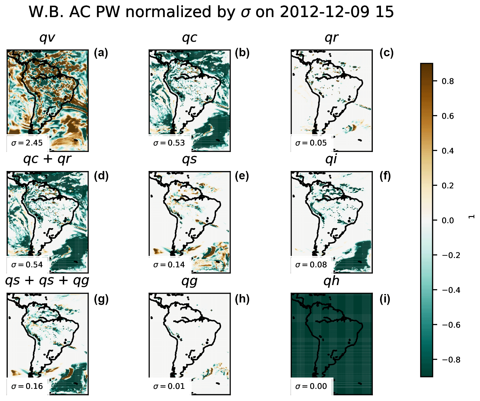
Figure 10Normalized (with the spatial standard deviation of the mapped values, σ) water budget 3 h accumulated vertically integrated total tendency PW at a given time, for water vapor (qv, a), cloud (qc, b), rain (qr, c), water condensed species (qc+qr, d), snow (qs, e), ice (qi, f), water solid species (qs+qi+qg, g), graupel (qg, h), and hail (qh, i). Numbers in the lower left corner of the panels correspond to the standard deviation (σ in millimeters) value used for the normalization.
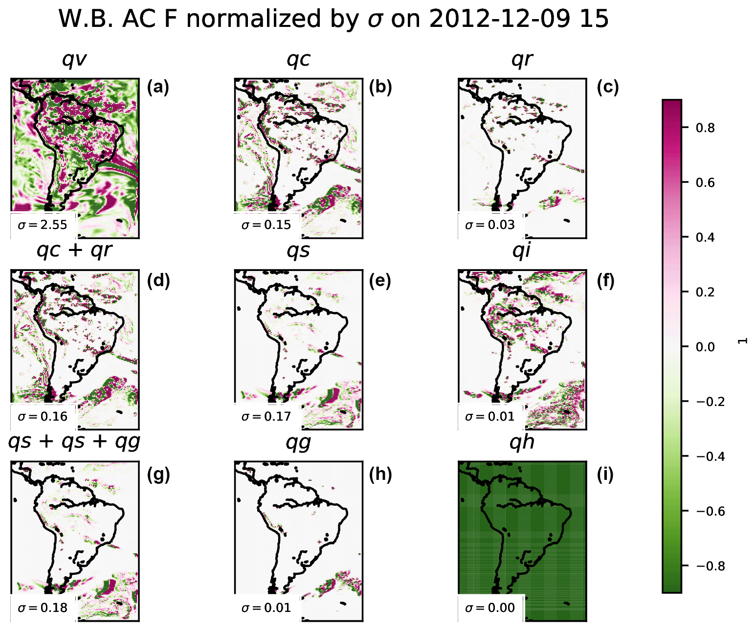
Figure 11As in Fig. 10, but for water budget 3 h accumulated vertically integrated horizontal advection F at a given time.
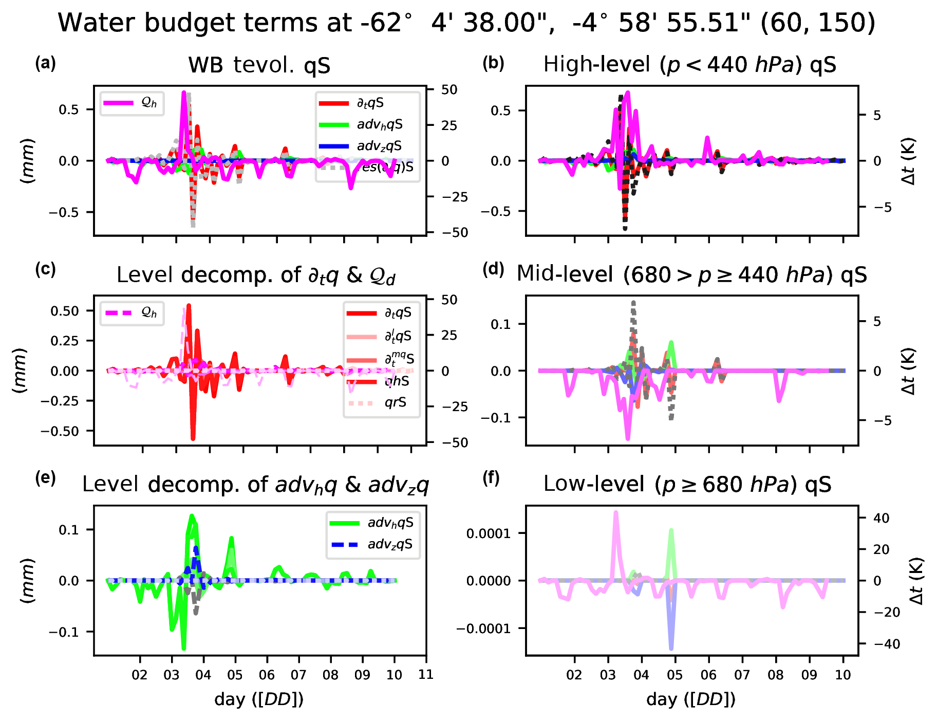
Following the methodology of Huang et al. (2014) and Yang et al. (2011), Fita and Flaounas (2018) implemented a new module in WRF in order to allow for the computation of the water budget terms during model integration. This implementation is provided with the CORDEX module, but these variables are only provided as temporal accumulations (within 9freq) and vertical integrations in two forms: total column values and divided by the same layers as the cloud diagnostics (low, medium, high). The accumulation of diabatic heating from the microphysics scheme is provided as a proxy for the sink and/or source due to microphysics effects.

Figure 12Water budget evolution at a given point for water vapor of vertically integrated water budget terms: total tendency PW (∂tqv, red), horizontal advection F (advhqv, green), vertical advection Z (advzqv, green), residual PW–F–Z (res(∂tqv), gray dashed), and diabatic heating from microphysics (𝒬d, pink) (a). Only high-level vertically integrated values (p<440 hPa, b), high-, mid-, and low-level (degree of color intensity) decomposition of ∂tqv (red) and 𝒬d (pink) and their respective residuals as dashed lines (c). Only mid-level vertically integrated values ( hPa, d), high-, mid-, and low-level (degree of color intensity) decomposition of advhqv (green) and advzqv (blue) and their respective residuals as dashed lines (e), and only low-level vertically integrated values (p≥680 hPa, f).
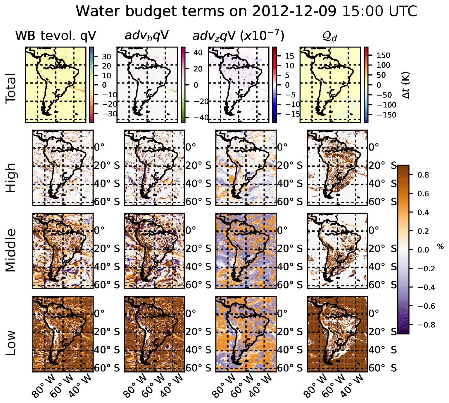
Figure 13Water vapor budget maps of each component and diabatic heating from microphysics at a given time and the percentage contribution at each different vertically integrated layer with respect to the total. Total tendency PW (∂tqv, first column), horizontal advection F (advhqv, second column), vertical advection Z (advzqv, third column), and diabatic heating from microphysics (𝒬d, fourth column). Percentage contribution of high-level (p<440 hPa) integration to the total (second row), percentage for mid-level ( hPa) integration to the total (third row), and percentage of low-level (p≥680 hPa) integration (bottom row).
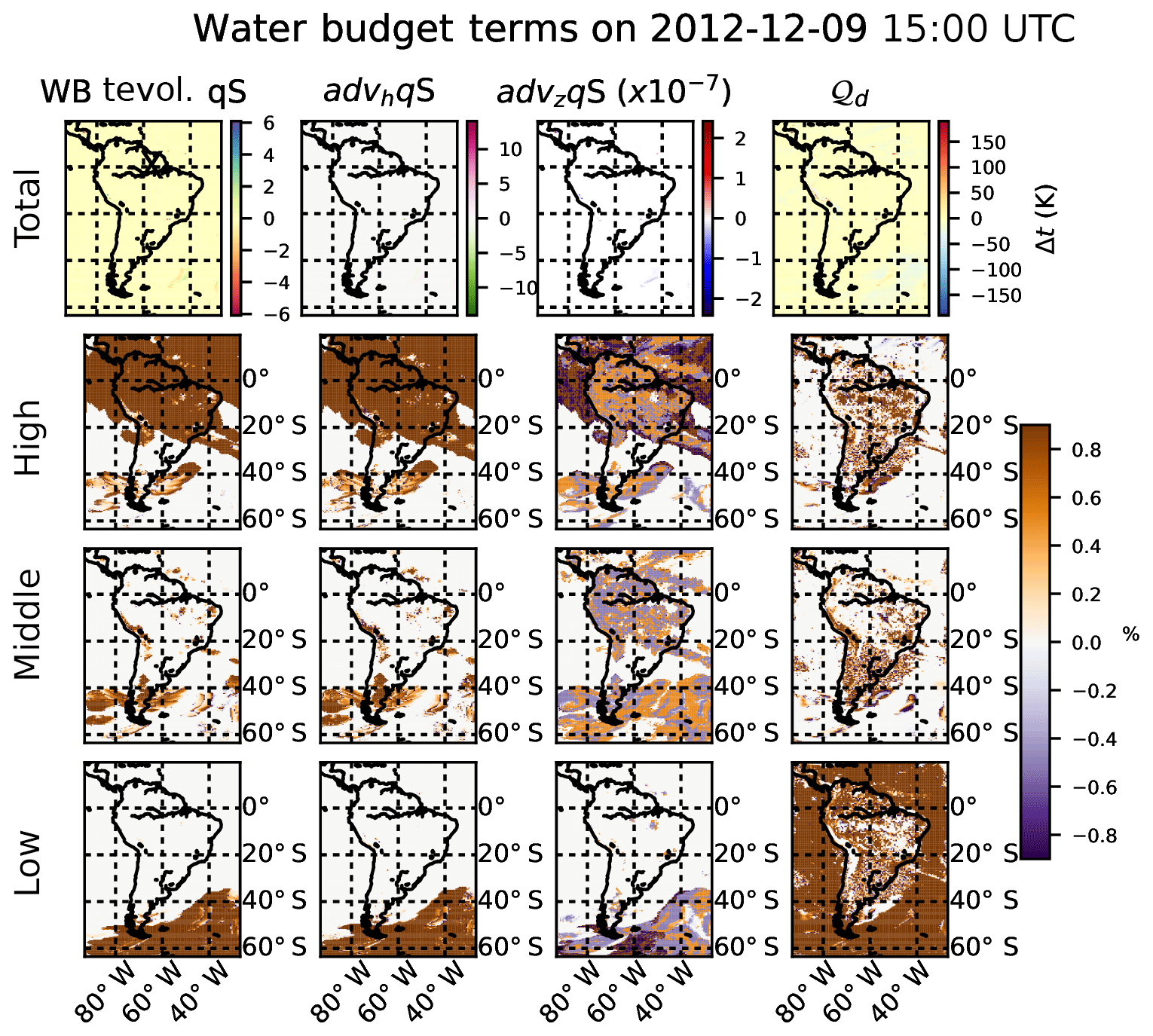
Preliminary results for all water species are shown in Figs. 10 and 11. Water vapor exhibits the largest values in both total tendency and horizontal advection. Dynamics of the other water species seems to be highly correlated with the presence of a storm system (lower right corner in the maps) or due to orthographic influences (the existence of the Andes mountain range can be inferred).
Figures 12 to 15 show temporal evolution and accumulated maps at a given time for all the water budget terms, decomposed for vapor (qv) and snow (qs). Accumulated maps are grouped into vertical levels as is done with the clouds: p≥68 000 Pa, Pa, p<40 000 Pa. The largest amounts of the budget terms are mainly found in low (high) levels for water vapor (snow); temporal evolution at a given point shows the complexity of the water dynamics, with the terms compensating for each other. Figures 12 to 15 also show how the contribution to the total diabatic term is large at low levels over the ocean (showing the role of evaporation) and larger at high levels above the continent.
fogvis: visibility inside fog
Fog is one of the major causes of transportation disruption. The horizontal resolutions of state-of-the-art CORDEX activities like FPS_Alps (3 km) open the possibility to explore phenomena such as fog, which was impossible to analyze in previous reginal climate experiments. In order to contribute to the analysis of fog phenomena, three different methods to calculate visibility have been introduced. Visibility is used to determine the presence of fog at a given moment. In order to provide a quantity with the density of the fog, only the visibility during a fog event is kept. The three methods are as follows (in italics).
-
K84
[visibility_diag = 1]. Visibility is computed using liquid water (QCLOUD) and ice (QICE) concentrations. Following Bergot et al. (2007), fog appears when there are liquid and/or ice water species at the lowest model level present. Visibility is computed using Eq. (31) as in Kunkel (1984):where QCLOUD is the liquid water (cloud) mixing ratio (kg kg−1), and QICE is the ice mixing ratio (kg kg−1). Visibility values are in kilometers.
-
RUC
[visibility_diag = 2]. Visibility is computed using relative humidity (hur) as implemented in the RUC model (see Eq. 32 from Smirnova et al., 2000):where hur is relative humidity (1, previously computed) and can be from the 2 m diagnostics or the first model layer. Visibility values are in kilometers.
-
FRAM-L
[visibility_diag = 3](default). Visibility is computed using relative humidity (hur) after Gultepe and Milbrandt (2010, see their Eq. 33). In this work, a probabilistic approach is proposed to compute the visibility in three different bins: 95 %, 50 %, and 5 % probability to get certain visibility (for hurs > 30 %). As a matter of compromise in the module, the calculation with 50 % probability has been chosen as the preferred one. Therefore, this method provides the visibility that may occur with 50 % probability:where RH is relative humidity and can be from 2 m diagnostics [hurs, in CF-notation] or the first model layer [hur(1)]. Visibility values are in kilometers.
The provided values of visibility during a fog event are the minimum,
maximum,
and mean values within output time steps (9freq) when fog occurred. Different
choices are controlled through namelist variables:
visibility_diag determines the method used to compute visibility,
and fogvars determines the source of the relative humidity to be used as
input in the visibility method. Users can choose between the relative humidity
from the first model layer (hur) fogvars=1 (default value) or from
the 2 m diagnostics (hurs) fogvars=2. Some preliminary results for
an extreme fog episode in central Argentina are provided in
Fig. 16. Results strongly differ among fog
implementations. The best agreement with a satellite-visible channel picture
for a given time of the event is obtained when the default setting is used
(FRAM-L method with hur values as input).
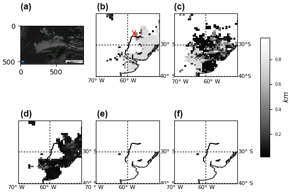
Figure 16On 30 June 2007 at 12:00 UTC, comparison of the different configurations of the diagnostics of mean fog visibility (in 1 h) to the satellite image from GOES-12 (a) at the same time in the visible channel (courtesy of NOAA-CLASS), default vis3vars1 (fogvisibility=3, fogvars=1; b), vis3vars2 (c), vis1vars1 (d), vis2vars1 (e), and vis2vars2 (f).
It is known that certain methods for calculating visibility rely on numerical adjustments to observational data taken under certain circumstances and at specific places (e.g., for FRAM-L, adjusted values come from observations from a Canadian airport). It would be desirable to provide a more generic “all places and purposes” approach (if possible). It is recommended to use this variable with care.
Regional climate dynamical downscaling experiments like the ones under the
scope of CORDEX require long continuous simulations that consume larger
amounts of HPC resources for a long period of time. Therefore, a series of
tests were carried out in order to investigate the impact on the time of
integration when the module is activated. The first version of the module (v1.0) was
known to introduce about a 40 % decrease in time-step speed of integration
(highly dependent on HPC, model configuration, and domain specifications). In
order to improve model performance when the module is activated, the module
was upgraded to version 1.1. Since this new version, a series of
optimizations of the code and pre-compilation flags have been activated
(CDXWRF). Following this implementation (instead of via regular WRF
namelist options), two main goals were achieved: (1) the amount of variables
kept in memory during model execution was reduced and (2) the number of
conditions (mainly avoiding IF statements) to be checked and calculations at
each execution step of integration was reduced as well.
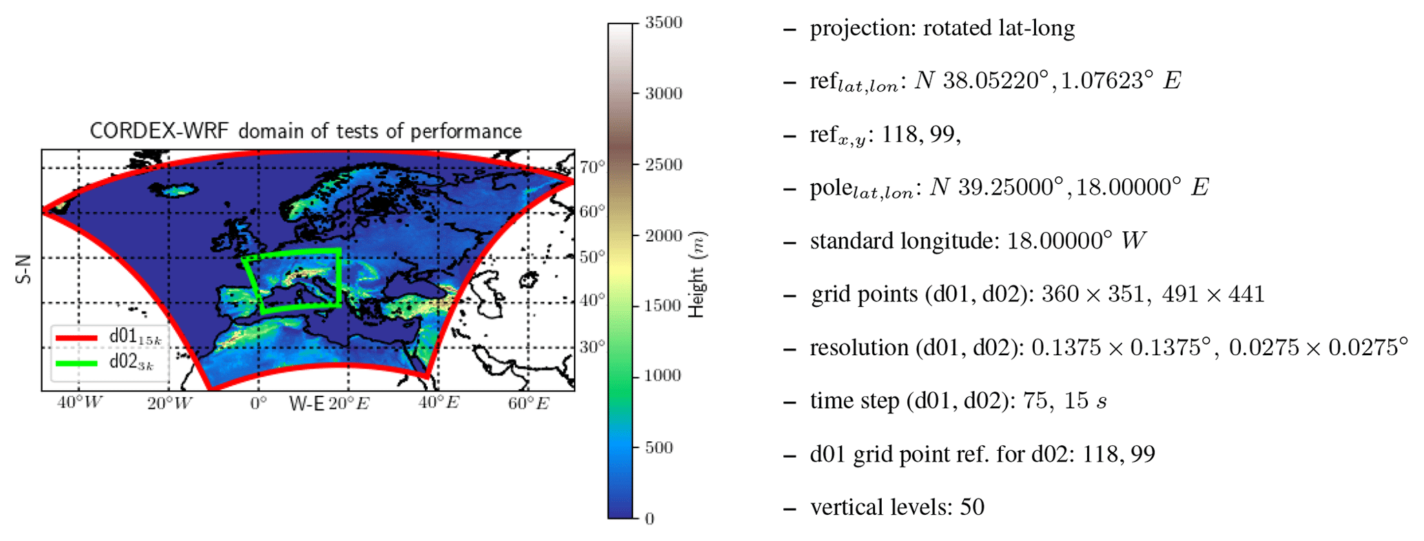
Figure 17Two-nested domain WRF3.8.1 configuration in which different performance tests were carried out.

Figure 18Elapsed times for each individual time-step integration on nested domain d02 (time steps from number 3800, simulating date 1 January 2014 15:35:00 UTC, to 4050 for 1 January 2014 16:37:30 UTC). Model was run with different module configurations. See text for more details. Larger time steps are related to activation of the shortwave and longwave radiation scheme (every 5 min). For WRF compilation using IFORT (a) and GCC compilers (b).
A domain as shown in Fig. 17 has been set up to perform short runs (5 days) to check the changes in performance of the WRF model when the module is activated in its different possible configurations. In order to avoid nonhomogeneous communication among the cluster nodes (which would affect the analysis), all the simulations were executed on a single node and with the WRF model compiled with Intel and GNU Fortran compilers. Tests are performed at the HPC Fram (https://www.sigma2.no/Fram, last access: 18 March 2019) from the Norwegian academic HPC infrastructure. Fram is based on Lenovo NeXtScale nx360, constituted by the CPU types Intel E5-2683v4 2.1 GHz and Intel E7-4850v4 2.1 GHz.
Table 4Mean elapsed time step of 5-day simulation and difference in time with respect to the original version of the code (v381orig) for different model configurations. See text for more details.

The execution time is calculated as the mean elapsed time used during the
5-day model integration. The elapsed time necessary for each simulation step is
available from the standard output of the model run
(rsl.error.0000
WRF ASCII file). In this file, WRF users can get the elapsed time for all the
time steps of the model and domains of simulation. Different peaks of slower
time steps (see in Fig. 18) coincide with input/output
file operations, differences between day and night regimes, and when different
physical schemes (mainly the radiative scheme) are activated at a given
frequency (e.g., radt). For a simulation covering 5 days with a time
step of 15 s, one obtains 28 800 time steps. The sample of 28 800 time
steps is considered to be large enough to be representative for the mean
time step of the whole simulation.
Table 4 describes the different configurations and
namelist options used in this performance test. The first simulation (labeled
v381orig), which is used as a reference, is the simulation with the original
version of the model (here version 3.8.1) without the module. The other
simulations are activation of the module (setting CORDEXDIAG) without
setting the pre-compilation parameter CDXWRF (labeled NOCDXWRF),
with pre-compilation parameter CDXWRF=1 (CDXWRF1), with
pre-compilation parameter CDXWRF=2, and computing all extra
calculations (CDXWRF2). Finally, three more simulations (with CDXWRF=2)
are made: without any extra calculation (CDXWRF2_00), without calculation of
extra water budget terms (CDXWRF2_01), and without extremes from convection
indices (CDXWRF2_10). Results might present some inconsistencies due to the
fact that certain computations of diagnostics depend on the stability at each
grid point, which might vary from run to run and depending on the workload of the HPC.
Results show that all the simulations (except CDXWRF1 with GCC) in which the
module has been activated are slower than the simulation with the original
version of the code (v381orig, s). Simulation with version 1.3 of the module without
pre-compilation flag CDXWRF (NOCDXWRF, s)
is the second fastest. Simulation becomes slower when all the extra
calculations are performed (CDXWRF2 s). The heaviest
part of the module is related to the water budget computation
(wb_diag=1), since when comparing to the simulation without extra
calculations (CDXWRF2_00, s) there is an increase
of only about 1, or 9 %
(,
),
of the mean time step when only statistics for extreme convective indices are
activated (CDXWRF2_01, s) and 27, or 19 %
(),
when only the water budget terms are included (CDXWRF2_10, s). Reduction of the time step for CDXWRF1 with GCC must be related to a
moment during which HPC Fram experiences a period of very low working load.
These results are not conclusive (optimization of the module should be tested
in other HPC resources, domains, and compilers), but they provide a first
insight on how the number of variables included during integration (in
the derived grid) has an important effect on model performance by
reducing or increasing the required amount of memory. CDXWRF1 and CDXWRF2_00
perform the same amount of computations of diagnostics, but the mean time
step in CDXWRF2_00 is almost doubled (because in the CDXWRF2_00 case all
the additional variables are defined but not diagnosed).
A series of modifications have been introduced into the WRF model in order to make it more suitable for CORDEX experiments. These modifications include the creation of a new module for the model and the modification of certain sections of the code. With the module implementation, users have the option to retrieve directly from the WRF output all the Core and almost all the Tier 1 CORDEX variables. Moreover, a series of additional variables not required by CORDEX, which may be of high interest to the regional climate modeling community, have been included. Additionally, a series of “generic” variables are provided that are independent of the model setup, which should allow for more robust intercomparisons.
A WRF user participating in a CORDEX regional climate experiment will strongly benefit when activating the module presented here, since it avoids most of the complex and time-consuming post-processing efforts necessary to obtain diagnostics required by CORDEX. Furthermore, the module makes use of the WRF online interpolation to pressure levels of certain three-dimensional variables, which is an expensive computational task. In addition, statistical values (like minimum fluxes or accumulation) are computed using the actual values obtained during the model integration. Since the use of the module avoids the post-processing of the model output, there is no need to keep large amounts of additional fields, which drastically reduces the requirements of disk storage (roughly 50 % less disk storage).
In order to reduce the impact of the module during model integration, the setup of the module is managed before the compilation of the model via pre-compilation flags. This reduces the requirements of memory since the calculation of only required variables is activated. Different tests showed that the model performance is significantly improved when the code and the variables are constrained to the required ones (and not all of those available) and managed via pre-compilation flags (and via conditional statements from the model namelist as is usually done in the WRF model).
The module also establishes a first attempt to provide and implement generic definitions of certain diagnostics directly from regular model fields. This specific effort is intended to provide diagnostics that would not depend on the model configuration and/or the model itself, which will make intercomparisons between models more accurate, generic, and trustworthy. If there is also a certain coordination (e.g., within the CORDEX community) of the definition of these diagnostics, climate studies will benefit. Common definitions of diagnostics in a coordinated way across different modeling platforms will ensure the robustness of model intercomparisons.
There are certain variables from CORDEX Tier 1 protocol, which are not yet introduced but required. These are (1) snowmelt, (2) the daily maximum wind speed of gusts at 100 m (wsgsmax100), which is not yet introduced because of a lack of an appropriate method, and (3) intra-cloud, ground, and total lightning flashes (ic_lightning, cg_lightning, tot_lightning), even though a lightning scheme is already implemented in WRF. However, this implementation is not appropriate for small domain patches used during parallelization. It has been found (Lluís Fita and Milagros Álvarez, CIMA personal communication, 2018) that lightning flash rates become patchy when the size of the parallel domain partitions are smaller than the actual extent of the cell. Lightning methods (Price and Rind, 1992; Wong et al., 2013) require encompassing the whole convective cell to analyze the updraft within the cell. When patches do not cover the whole cell, different values from the same cell at each parallel fraction of the domain are provided, from which spatial inconsistencies arise.
The module provides almost all the required CORDEX variables. However, users still need to perform some post-processing of the output data in order to meet CORDEX standards, mainly the following:
-
computation of the required different statistical values as daily, monthly and seasonal extremes (minimum, maximum, accumulations, means); and
-
cmorization of the output understood as one file per variable, the right metadata and attributes, and general CF-compliant standard specifications.
There are some additional features that would make the module more useful for the climate regional community, which are also required by the CORDEX specifications. However, in order to prioritize the production of a basic, fully working, and useful version of the module as soon as possible, the following aspects are planned for future iterations and updates.
-
Flexibility enhancement is needed in terms of the capacity to provide a more flexible module that is easy to maintain and update with new requirements from CORDEX or WRF model updates.
-
Introduce new variables with a special focus on the implementation of more generic variable definitions
-
CF-compliant and cmorization output is needed because WRF output does not fully follow CF conventions. Thus, a huge coding effort is needed to provide fully CF-compliant output directly from it. Users still need to process the output of the model in order to provide data following all the CORDEX guidelines. Due to uncovered steps of the CF standard, a user of the WRF model still needs to concatenate files, change the names and attributes of variables, calculate temporal statistics over different periods (daily, monthly, seasonal), and provide the right time variables in order to fully reach the CF standard followed by CORDEX. However, these steps are computationally lighter and easier to perform in comparison to the computation of the different diagnostics and the vertical pressure interpolation already introduced in the module.
The incompatibility between WRF output and CF conventions can be overcome with the use of a complementary dedicated I/O library. This has been done, for example, on the RegIPSL platform (https://sourcesup.renater.fr/wiki/morcemed/Home, which uses WRF as an atmospheric model), which uses XIOS (http://forge.ipsl.jussieu.fr/ioserver, last access: 18 March 2019) libraries to manage the I/O.
The module is currently being implemented in the repository of the code in a dedicated branch. Once the module is fully implemented in the latest version of the model, and some additional tests are conducted, it might be possible that the model developing team decides to include it in the main source of the code.
The discussed version of the module (1.3) in the present article for four different WRF versions is available through the following digital object identifiers (DOIs).
-
WRF-CORDEX module version 1.3 for WRFV3.7.1: https://doi.org/10.5281/zenodo.1469639 (Fita et al., 2018a)
-
WRF-CORDEX module version 1.3 for WRFV3.8.1: https://doi.org/10.5281/zenodo.1469645 (Fita et al., 2018b)
-
WRF-CORDEX module version 1.3 for WRFV3.9.1.1: https://doi.org/10.5281/zenodo.1469647 (Fita et al., 2018c)
-
WRF-CORDEX module version 1.3 for WRFV4.0: https://doi.org/10.5281/zenodo.1469651 (Fita et al., 2018d)
It is strongly recommended to make contact with lluis.fita@cima.fcen.uba.ar. This would facilitate the creation of a community of users of the module and make it easier to share updates and improvements with users.
A Wiki page has been set up in order to provide detailed instructions on how to manage the module and to give information about upcoming module versions and improvements. The page will be regularly updated and can be found at http://wiki.cima.fcen.uba.ar/mediawiki/index.php/CDXWRF (last access: 18 March 2019).
A generic list of requested variables by CORDEX is provided here. The reader is advised that there is not a single list of CORDEX requirement variables. It might depend on the experiment. However, with the aim of providing a generic list of variables, the CORDEX requirements are presented in Table A1. The source of the table is the ESGF servers at https://www.earthsystemcog.org/doc/detail/1065/ (last access: 18 March 2019). The same variables might appear at different levels (Core, Tier 1, Tier 2) as a function of the requested frequency and/or if they should be provided as statistical values between output frequency or instantaneous values, as well as depending on the experiment (FPS_Alps experiment requested additional variables provided in Table A2).
Table A1CORDEX requested variables (from https://www.earthsystemcog.org/doc/detail/1065/). Ovarn: variable output name, L: level of requirement (c, Core; 1, Tier 1; 2, Tier 2), activation: option to get the variable from WRF (wrfout, standard WRF output; clwrf, after clWRF modifications; cdxdiag, basic CORDEXDIAG compilation; cdxwrf1, CORDEXDIAG activating pre-compilation flag cdxwrf=1; cdxwrf2, CORDEXDIAG activating pre-compilation flag cdxwrf=2; not available, not retrievable in this version of the module), ∗ indicates when a variable has a dependency on the chosen scheme.

∗ Scheme dependant.
Table A2As in Table A1, but for the additional variables requested by the CORDEX FPS_Alps experiment.
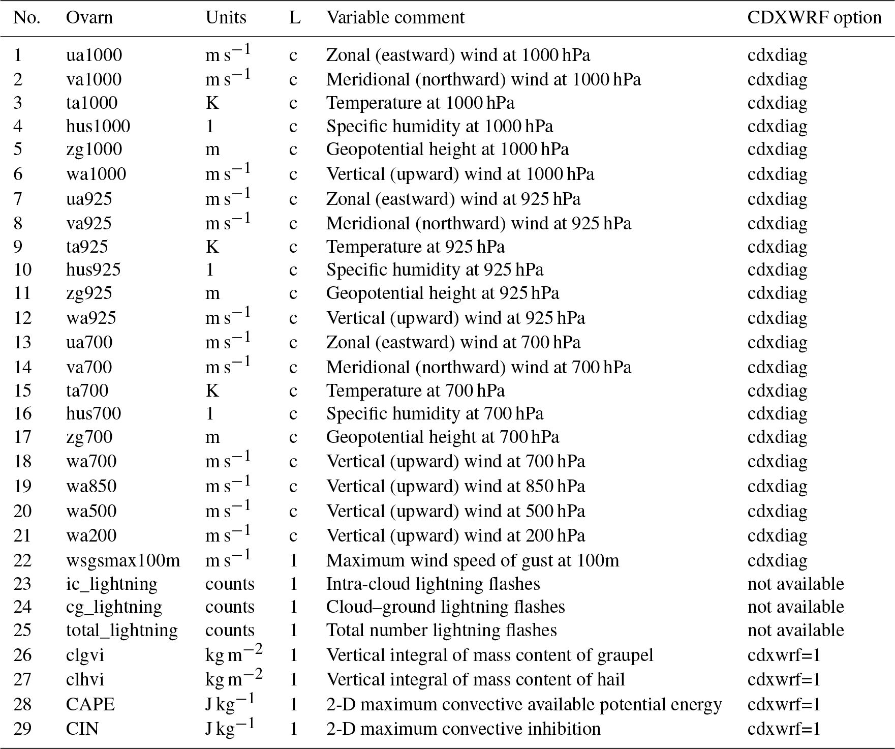
B1 Core variables
The variables given in Table B1
are always provided when the module is activated with the use of the
pre-compilation flag CORDEXDIAG. These variables appear in the
auxiliary output file number 9. It is recommended to set the name of this
file as wrfcdx_d<domain>_<date>. Note that some variables might not be
produced according to chosen namelist options.
B2 Tier 1
The variables given in Table B2 are provided if the
preprocessing variable CDXWRF is set to 1. These variables also appear
in the auxiliary output file number 9. Note that some variables might not be
produced according to chosen namelist options.
B3 Additional
The variables from Table B3 are provided if the preprocessing variable
CDXWRF is set to 2. These variables also appear in the auxiliary
output file number 9. Note that some variables might not be produced
according to chosen namelist options.
B4 Instantaneous
The variables given in Table B4 are provided if some modifications are made in the WRF code. These variables represent instantaneous values for a certain number of variables that are internally used. These variables also appear in the auxiliary output file number 9. Note that some variables might not be produced according to chosen namelist options.
Table B1Description of CORDEX Core variables provided with the module. “Kind” specifies when the variable is computed; a: computed all time steps, o: only at output time, t: according to a frequency in the namelist, s: statistic value from internal integration values and initialized after each output time step.

a Needed for other variables. b Unmasked to sea points.
Table B2As in Table B1, but for the description of CORDEX Tier 1 variables provided with the module.

It will be computed if the namelist parameter convxtrm_diag is set to 1.
Table B3As in Table B1, but for the description of additional variables provided with the module.
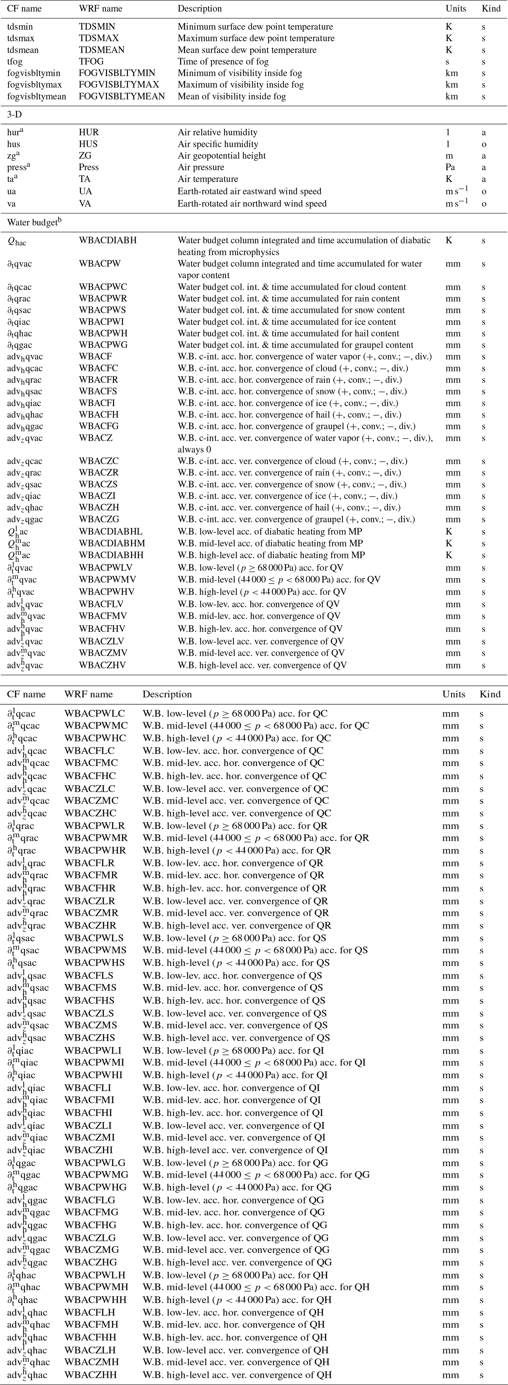
a Needed for other variables. b Variables will be computed if the namelist parameter output_wb is set to 1.
Table B4As in Table B1, but for the description of CORDEX “instantaneous” variables provided with the module.
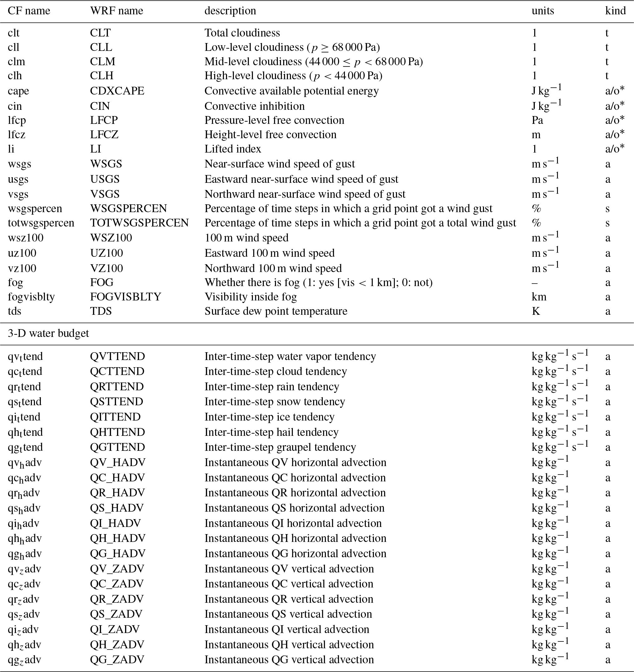
∗ Depending on namelist parameter
convxtrm_diag 0:o, 1:a.
All authors contributed to revising the paper. At the same time, the authors carried out different tasks in the study.
LF contributed to the study by developing the code of the module, implementing it in the different versions of WRF, and performing some model simulations in order to test the module and obtain the necessary data for the different figures. He was in charge of the text of the paper, created all the figures, and obtained the different DOIs. JP contributed by testing the outcomes of the module in parallel simulations and provided some advice on the implementation of diagnostics such as potential evapotranspiration. TMG contributed by revising the implementation of the first versions of the module. TL contributed by making the different simulations needed to test the performance of the module. JM contributed by detecting some flaws in the module through independent simulations. GS revised the definition of the variables in the module by checking their agreement with the CF conventions. EK and SB made important contributions to the text of the paper and other details in the development of the code for the module.
The authors declare that they have no conflict of interest.
All the coders of WRF, LMDZ, and ORCHIDEE models are acknowledged for their hard work on developing and maintaining the models. Maria Antònia Jiménez from the Universitat de les Illes Balears is acknowledged for her explanations on certain PBL calculations. Daniel Argüeso from UIB and Victoria Galligani, Juan Ruiz, and Mariano Sebastián from CIMA are also acknowledged for their commentaries. Anna Sörensson and Elsa Borrell are also acknowledged for their assistance. Implementation tests were performed at the CIMA HPC resources “hydra” cluster supported by the High Performance Computing National System (SNCAD) of Argentina. Lluís Fita thanks the CIMA IT support staff for their work. Eleni Katragkou and Giannis Sofiadis acknowledge the technical support and provision of resources from the Scientific Computing Center of AUTH (https://it.auth.gr/el, last access: 18 March 2019) and the GRNET National HPC infrastructure (https://hpc.grnet.gr/, last access: 18 March 2019). Josipa Milovac gratefully acknowledges support from the German Science Foundation (DFG) through project FOR 1695 and the supercomputing center HLRS in Stuttgart, Germany, for granting the computing time necessary for the test simulations. Torge Lorenz acknowledges support from the Research Council of Norway and its basic institute support of the strategic project on climate services. The simulations were performed on resources provided by UNINETT Sigma2 – the National Infrastructure for High Performance Computing and Data Storage in Norway. Figures were produced with Python (except performance tests drawn with GNUplot), and Lluís Fita thanks the development team of Matplotlib with which he developed and made available a suite in Python for NetCDF management and plotting purposes called PyNCplot (available from http://www.xn–llusfb-5va.cat/python/PyNCplot, last access: 18 March 2019). The authors are grateful for the commentaries of the topical editor (Jatin Kala), which remarkably improved the paper.
This paper was edited by Jatin Kala and reviewed by two anonymous referees.
Barella-Ortiz, A., Polcher, J., Tuzet, A., and Laval, K.: Potential evaporation estimation through an unstressed surface-energy balance and its sensitivity to climate change, Hydrol. Earth Syst. Sci., 17, 4625–4639, https://doi.org/10.5194/hess-17-4625-2013, 2013. a
Benjamin, S. G. and Miller, P. A.: An Alternative Sea Level Pressure Reduction and a Statistical Comparison of Geostrophic Wind Estimates with Observed Surface Winds, Mon. Weather Rev., 118, 2099–2116, https://doi.org/10.1175/1520-0493(1990)118<2099:AASLPR>2.0.CO;2, 1990. a, b
Bergot, T., Terradellas, E., Cuxart, J., Mira, A., Liechti, O., Mueller, M., and Nielsen, N. W.: Intercomparison of Single-Column Numerical Models for the Prediction of Radiation Fog, J. Appl. Meteorol. Clim., 46, 504–521, https://doi.org/10.1175/JAM2475.1, 2007. a
Brasseur, O.: Development and Application of a Physical Approach to Estimating Wind Gusts, Mon. Weather Rev., 129, 5–25, https://doi.org/10.1175/1520-0493(2001)129<0005:DAAOAP>2.0.CO;2, 2001. a, b
Businger, J. A., Wyngaard, J. C., Izumi, Y., and Bradley, E. F.: Flux-Profile Relationships in the Atmospheric Surface Layer, J. Atmos. Sci., 28, 181–189, https://doi.org/10.1175/1520-0469(1971)028<0181:FPRITA>2.0.CO;2, 1971. a
Coppola, E., Sobolowski, S., Pichelli, E., Raffaele, F., Ahrens, B., Anders, I., Ban, N., Bastin, S., Belda, M., Belusic, D., Caldas-Alvarez, A., Cardoso, R. M., Davolio, S., Dobler, A., Fernández, J., Fita, L., Fumiere, Q., Giorgi, F., Goergen, K., Guettler, I., Halenka, T., Heinzeller, D., Hodnebrog, O., Jacob, D., Kartsios, S., Katragkou, E., Kendon, E., Khodayar, S., Kunstmann, H., Knist, S., Lavín, A., Lind, P., Lorenz, T., Maraun, D., Marelle, L., van Meijgaard, E., Milovac, J., Myhre, G., H.-J.Panitz, Piazza, M., Raffa, M., Raub, T., Rockel, B., Schär, C., Sieck, K., Soares, P. M. M., Somot, S., Srnec, L., Stocchi, P., Tölle, M., Truhetz, H., Vautard, R., de Vries, H., and Warrach-Sagi, K.: A first-of-its-kind multi-model convection permitting ensemble for investigating convective phenomena over Europe and the Mediterranean, Clim. Dynam., e-print first, https://doi.org/10.1007/s00382-018-4521-8, 2018. a
de Rosnay, P., Polcher, J., Bruen, M., and Laval, K.: Impact of a physically based soil water flow and soil-plant interaction representation for modeling large-scale land surface processes, J. Geophys. Res.-Atmos., 107, 4118, https://doi.org/10.1029/2001JD000634, 2002. a
Domínguez, M., Romera, R., Sánchez, E., Fita, L., Fernández, J., Jiménez-Guerrero, P., Montávez, J. P., Cabos, W. D., Liguori, G., and Gaertner, M. A.: Present climate precipitation and temperature extremes over Spain from a set of high resolution RCMs, Clim. Res., 58, 149–164, https://doi.org/10.3354/cr01186, 2013. a
Evans, J. P., Ji, F., Lee, C., Smith, P., Argüeso, D., and Fita, L.: Design of a regional climate modelling projection ensemble experiment – NARCliM, Geosci. Model Dev., 7, 621–629, https://doi.org/10.5194/gmd-7-621-2014, 2014. a
Fita, L. and Flaounas, E.: Medicanes as subtropical cyclones: the December 2005 case from the perspective of surface pressure tendency diagnostics and atmospheric water budget, Q. J. Roy. Meteor. Soc., 144, 1028–1044, https://doi.org/10.1002/qj.3273, qJ-17-0198.R2, 2018. a, b
Fita, L., Fernández, J., and García-Díez, M.: CLWRF: WRF modifications for regional climate simulation under future scenarios, Proceedings of 11th WRF Users' Workshop, 22–24 June 2010, Boulder, Colorado, USA, 2010. a, b, c
Fita, L., Polcher, J., and Giannaros, T. M.: WRF-CORDEX module version 1.3 for WRFV3.7.1, https://doi.org/10.5281/zenodo.1469639, 2018a. a
Fita, L., Polcher, J., and Giannaros, T. M.: WRF-CORDEX module version 1.3 for WRFV3.8.1, https://doi.org/10.5281/zenodo.1469645, 2018b. a
Fita, L., Polcher, J., and Giannaros, T. M.: WRF-CORDEX module version 1.3 for WRFV3.9.1.1, https://doi.org/10.5281/zenodo.1469647, 2018c. a
Fita, L., Polcher, J., and Giannaros, T. M.: WRF-CORDEX module version 1.3 for WRFV4.0, https://doi.org/10.5281/zenodo.1469651, 2018d. a
Fu, C., Wang, S., Xiong, Z., Gutowski, W. J., Lee, D. K., McGregor, J. L., Sato, Y., Kato, H., Kim, J. W., and Suh, M. S.: Regional climate model intercomparison project for Asia, B. Am. Meteorol. Soc., 86, 257–266, 2005. a
García-Díez, M., Fernández, J., Fita, L., and Yagüe, C.: Seasonal dependence of WRF model biases and sensitivity to PBL schemes over Europe, Q. J. Roy. Meteor. Soc., 139, 501–514, https://doi.org/10.1002/qj.1976, 2013. a
Garratt, J.: The Atmospheric Boundary Layer, Cambridge Univ. Press, Cambridge, UK, 1992. a
Geleyn, J. F. and Hollingsworth, A.: An economical analytical method for the computation of the interaction between scattering and line absorption of radiation, Contrib. Atmos. Phys, 52, 1–16, 1979. a
Giorgi, F. and Gutowski, W. J.: Regional Dynamical Downscaling and the CORDEX Initiative, Annu. Rev. Env. Resour., 40, 467–490, https://doi.org/10.1146/annurev-environ-102014-021217, 2015. a
Giorgi, F. and Mearns, L. O.: Approaches to the simulation of regional climate change: A review, Rev. Geophys., 29, 191–216, https://doi.org/10.1029/90RG02636, 1991. a
Giorgi, F., Jones, C., and Asrar, G.: Addressing climate information needs at the regional level: the CORDEX framework, WMO Buletin, 58, 175–183, 2009. a
Gultepe, I. and Milbrandt, J. A.: Probabilistic Parameterizations of Visibility Using Observations of Rain Precipitation Rate, Relative Humidity, and Visibility, J. Appl. Meteorol. Clim., 49, 36–46, https://doi.org/10.1175/2009JAMC1927.1, 2010. a, b
Hourdin, F., Musat, I., Bony, S., Braconnot, P., Codron, F., Dufresne, J.-L., Fairhead, L., Filiberti, M.-A., Friedlingstein, P., Grandpeix, J.-Y., Krinner, G., LeVan, P., Li, Z.-X., and Lott, F.: The LMDZ4 general circulation model: climate performance and sensitivity to parametrized physics with emphasis on tropical convection, Clim. Dynam., 27, 787–813, https://doi.org/10.1007/s00382-006-0158-0, 2006. a
Huang, H.-L., Yang, M.-J., and Sui, C.-H.: Water Budget and Precipitation Efficiency of Typhoon Morakot (2009), J. Atmos. Sci., 71, 112–129, https://doi.org/10.1175/JAS-D-13-053.1, 2014. a
Jaeger, E. B. and Seneviratne, S. I.: Impact of soil moisture–atmosphere coupling on European climate extremes and trends in a regional climate model, Clim. Dynam., 36, 1919–1939, https://doi.org/10.1007/s00382-010-0780-8, 2011. a
Jourdier, B.: Ressource éolienne en France métropolitaine: méthodes d'evaluation du potentiel, variabilité et tendances, Climatologie: École Doctorale Polytechnique, 2015. Français, Palaisseau, France, 1–229, 2015. a
Katragkou, E., García-Díez, M., Vautard, R., Sobolowski, S., Zanis, P., Alexandri, G., Cardoso, R. M., Colette, A., Fernandez, J., Gobiet, A., Goergen, K., Karacostas, T., Knist, S., Mayer, S., Soares, P. M. M., Pytharoulis, I., Tegoulias, I., Tsikerdekis, A., and Jacob, D.: Regional climate hindcast simulations within EURO-CORDEX: evaluation of a WRF multi-physics ensemble, Geosci. Model Dev., 8, 603–618, https://doi.org/10.5194/gmd-8-603-2015, 2015. a
Knist, S., Goergen, K., Buonomo, E., Christensen, O. B., Colette, A., Cardoso, R. M., Fealy, R., Fernández, J., García-Díez, M., Jacob, D., Kartsios, S., Katragkou, E., Keuler, K., Mayer, S., Meijgaard, E., Nikulin, G., Soares, P. M. M., Sobolowski, S., Szepszo, G., Teichmann, C., Vautard, R., Warrach-Sagi, K., Wulfmeyer, V., and Simmer, C.: Land-atmosphere coupling in EURO-CORDEX evaluation experiments, J. Geophys. Res.-Atmos., 122, 79–103, https://doi.org/10.1002/2016JD025476, 2014. a
Kotlarski, S., Keuler, K., Christensen, O. B., Colette, A., Déqué, M., Gobiet, A., Goergen, K., Jacob, D., Lüthi, D., van Meijgaard, E., Nikulin, G., Schär, C., Teichmann, C., Vautard, R., Warrach-Sagi, K., and Wulfmeyer, V.: Regional climate modeling on European scales: a joint standard evaluation of the EURO-CORDEX RCM ensemble, Geosci. Model Dev., 7, 1297–1333, https://doi.org/10.5194/gmd-7-1297-2014, 2014. a
Kunkel, B. A.: Parameterization of Droplet Terminal Velocity and Extinction Coefficient in Fog Models, J. Clim. Appl. Meteorol., 23, 34–41, https://doi.org/10.1175/1520-0450(1984)023<0034:PODTVA>2.0.CO;2, 1984. a, b
Lawrence, D. M., Oleson, K. W., Flanner, M. G., Thornton, P. E., Swenson, S. C., Lawrence, P. J., Zeng, X., Yang, Z.-L., Levis, S., Sakaguchi, K., Bonan, G. B., and Slater, A. G.: Parameterization improvements and functional and structural advances in Version 4 of the Community Land Model, J. Adv. Model. Earth Syst., 3, M03001, https://doi.org/10.1029/2011MS00045, 2011. a
Manabe, S.: Climate and the ocean circulation, 1. the atmospheric circulation and the hydrology of the earth's surface, Mon. Weather Rev., 97, 739–774, https://doi.org/10.1175/1520-0493(1969)097<0739:CATOC>2.3.CO;2, 1969. a, b, c
Mearns, L., Gutowski, W. J., Jones, R., Leung, R., McGinnis, S., Nunes, A., and Qian, Y.: A regional climate change assessment program for North America, EOS Transactions AGU, 90, 311–312, https://doi.org/10.1029/2009EO360002, 2009. a
Milly, P. C. D.: Potential Evaporation and Soil Moisture in General Circulation Models, J. Climate, 5, 209–226, https://doi.org/10.1175/1520-0442(1992)005<0209:PEASMI>2.0.CO;2, 1992. a, b
Nakanishi, M. and Niino, H.: An Improved Mellor-Yamada Level-3 Model: Its Numerical Stability and Application to a Regional Prediction of Advection Fog, Bound.-Lay. Meteorol., 119, 397–407, https://doi.org/10.1007/s10546-005-9030-8, 2006. a
Nielsen-Gammon, J. W., Powell, C. L., Mahoney, M. J., Angevine, W. M., Senff, C., White, A., Berkowitz, C., Doran, C., and Knupp, K.: Multisensor Estimation of Mixing Heights over a Coastal City, J. Appl. Meteorol. Clim., 47, 27–43, https://doi.org/10.1175/2007JAMC1503.1, 2008. a, b
Nikulin, G., Jones, C., Giorgi, F., Asrar, G., Büchner, M., Cerezo-Mota, R., Christensen, O. B., Déqué, M., Fernández, J., Hänsler, A., van Meijgaard, E., Samuelsson, P., Sylla, M. B., and Sushama, L.: Precipitation Climatology in an Ensemble of CORDEX-Africa Regional Climate Simulations, J. Climate, 25, 6057–6078, https://doi.org/10.1175/JCLI-D-11-00375.1 2012. a
Oleson, K. W., Lawrence, D. M., B, G., Flanner, M. G., Kluzek, E., J, P., Levis, S., Swenson, S. C., Thornton, E., Feddema, J., Heald, C. L., Lamarque, J.-F., Niu, G.-Y., Qian, T., Running, S., Sakaguchi, K., Yang, L., Zeng, X., Zeng, X., and Decker, M.: Technical Description of version 4.0 of the Community Land Model (CLM), NCAR Technical Note NCAR/TN-478+STR, https://doi.org/10.5065/D6FB50WZ, 2010. a
Price, C. and Rind, D.: A simple lightning parameterization for calculating global lightning distributions, J. Geophys. Res.-Atmos., 97, 9919–9933, https://doi.org/10.1029/92JD00719, 1992. a
Ruti, P. M., Somot, S., Giorgi, F., Dubois, C., Flaounas, E., Obermann, A., Dell'Aquila, A., Pisacane, G., Harzallah, A., Lombardi, E., Ahrens, B., Akhtar, N., Alias, A., Arsouze, T., Aznar, R., Bastin, S., Bartholy, J., Béranger, K., Beuvier, J., Bouffies-Cloché, S., Brauch, J., Cabos, W., Calmanti, S., Calvet, J.-C., Carillo, A., Conte, D., Coppola, E., Djurdjevic, V., Drobinski, P., Elizalde-Arellano, A., Gaertner, M., Galàn, P., Gallardo, C., Gualdi, S., Goncalves, M., Jorba, O., Jordà, G., L'Heveder, B., Lebeaupin-Brossier, C., Li, L., Liguori, G., Lionello, P., Maciàs, D., Nabat, P., Önol, B., Raikovic, B., Ramage, K., Sevault, F., Sannino, G., Struglia, M. V., Sanna, A., Torma, C., and Vervatis, V.: Med-CORDEX Initiative for Mediterranean Climate Studies, B. Am. Meteorol. Soc., 97, 1187–1208, https://doi.org/10.1175/BAMS-D-14-00176.1, 2016. a
Skamarock, W. C., Klemp, J. B., Dudhia, J., Gill, D. O., Duda, D. M. B. M. G., Huang, X.-Y., Wang, W., and Powers, J. G.: A Description of the Advanced Research WRF Version 3, NCAR TECHNICAL NOTE, 475, NCAR/TN475+STR, Boulder, Colorado, USA, 2008. a, b, c
Smirnova, T. G., Benjamin, S. G., and Brown, J. M.: Case study verification of RUC/MAPS fog and visibility forecasts, Preprints, 9 th Conference on Aviation, Range, and Aerospace Meteorlogy, AMS, Orlando, FL, USA, 11–16 September 2000, 2.3, 31–36, 2000. a, b
Stackpole, J. and Cooley, D. S.: Revised method of 1000 mb height computations in the PE model, Technical Procedures Bulletin. U.S. Dept. of Commerce, National Oceanic and Atmospheric Administration, National Weather Service, NOAA Library, Silver Spring, MD, USA, 57, 6, 1970. a, b
Vautard, R., Gobiet, A., Jacob, D., Belda, M., Colette, A., Déqué, M., Fernández, J., García-Díez, M., Goergen, K., Güttler, I., Halenka, T., Karacostas, T., Katragkou, E., Keuler, K., Kotlarski, S., Mayer, S., van Meijgaard, E., Nikulin, G., Patarčić, M., Scinocca, J., Sobolowski, S., Suklitsch, M., Teichmann, C., Warrach-Sagi, K., Wulfmeyer, V., and Yiou, P.: The simulation of European heat waves from an ensemble of regional climate models within the EURO-CORDEX project, Clim. Dynam., 41, 2555–2575, https://doi.org/10.1007/s00382-013-1714-z, 2013. a
WMO: Manual on the Global Observing System, WMO, Geneva, Switzerland, 544, 2010a. a
WMO: Guide to Meteorological Instruments and Methods of Observation, Weather–Climate–Weather, Geneva, Switzerland, 1–176, 2010b. a
Wong, J., Barth, M. C., and Noone, D.: Evaluating a lightning parameterization based on cloud-top height for mesoscale numerical model simulations, Geosci. Model Dev., 6, 429–443, https://doi.org/10.5194/gmd-6-429-2013, 2013. a
Yang, M. J., Braun, S. A., and Chen, D.-S.: Water Budget of Typhoon Nari (2001), Mon. Wather Rev., 139, 3809–3828, https://doi.org/10.1175/MWR-D-10-05090.1, 2011. a
Yesad, K.: FULL-POS in the Cycle 41T1 of ARPEGE/IFS, Tech. Rep., Meteo-France, 45, available at: https://www.umr-cnrm.fr/gmapdoc/IMG/pdf/ykfpos43.pdf (last access: last access: 18 March 2019), 2015. a, b
From the AMS glossary at http://glossary.ametsoc.org/wiki/Specific_humidity (last access: 18 March 2019).
genericand
additionalones.