the Creative Commons Attribution 4.0 License.
the Creative Commons Attribution 4.0 License.
 | 09 Mar 2018
Autocalibration of a one-dimensional hydrodynamic-ecological model (DYRESM 4.0-CAEDYM 3.1) using a Monte Carlo approach: simulations of hypoxic events in a polymictic lake
Liancong Luo
David Hamilton
Jia Lan
Chris McBride
Dennis Trolle
Automated calibration of complex deterministic water quality models with a large number of biogeochemical parameters can reduce time-consuming iterative simulations involving empirical judgements of model fit. We undertook autocalibration of the one-dimensional hydrodynamic-ecological lake model DYRESM-CAEDYM, using a Monte Carlo sampling (MCS) method, in order to test the applicability of this procedure for shallow, polymictic Lake Rotorua (New Zealand). The calibration procedure involved independently minimizing the root-mean-square error (RMSE), maximizing the Pearson correlation coefficient (r) and Nash–Sutcliffe efficient coefficient (Nr) for comparisons of model state variables against measured data. An assigned number of parameter permutations was used for 10 000 simulation iterations. The “optimal” temperature calibration produced a RMSE of 0.54 ∘C, Nr value of 0.99, and r value of 0.98 through the whole water column based on comparisons with 540 observed water temperatures collected between 13 July 2007 and 13 January 2009. The modeled bottom dissolved oxygen concentration (20.5 m below surface) was compared with 467 available observations. The calculated RMSE of the simulations compared with the measurements was 1.78 mg L−1, the Nr value was 0.75, and the r value was 0.87. The autocalibrated model was further tested for an independent data set by simulating bottom-water hypoxia events from 15 January 2009 to 8 June 2011 (875 days). This verification produced an accurate simulation of five hypoxic events corresponding to DO < 2 mg L−1 during summer of 2009–2011. The RMSE was 2.07 mg L−1, Nr value 0.62, and r value of 0.81, based on the available data set of 738 days. The autocalibration software of DYRESM-CAEDYM developed here is substantially less time-consuming and more efficient in parameter optimization than traditional manual calibration which has been the standard tool practiced for similar complex water quality models.
- Article
(2304 KB) - Full-text XML
-
Supplement
(177 KB) - BibTeX
- EndNote


Water quality models provide an important framework for scientific assessment to support water quality management decision making (Stow et al., 2007; Schmolke et al., 2010) and test the future climatic impacts on aquatic ecosystems (Elliott, 2012; Tang et al., 2015). They can help in understanding processes operating at a wide variety of temporal and spatial scales, such as the mechanisms contributing to algal blooms, resuspension of sediments, and climate impacts on water quality (Asaeda et al., 2001; Robson and Hamilton, 2004, Chung et al., 2009; Pierson et al., 2013). Process-based water quality models use process representations of the major physical and biogeochemical processes in order to simulate observed data and to forecast changes that may occur under scenarios with changed forcings, for example, altered hydrology or climate (Cox, 2003; Whitehead et al., 2009). There have been many applications of coupled hydrodynamic-ecological models for assessments of surface water quality, including DYRESM-CAEDYM (Han et al., 2000; Asaeda et al., 2001; Copetti et al., 2006; Tanentzap et al., 2008; Takkouk and Casamitjana, 2016), ELCOM-CAEDYM (Vilhena et al., 2010; Chung et al., 2014; Mosley et al., 2015), EFDC (Li et al., 2013a; Alarcon et al., 2014), QUAL2Kw (Pelletier et al., 2006; Kannel et al., 2007a; Marsili-Libelli and Giusti, 2008), PCLake (Hu et al., 2016) and SWAT (Santhi et al., 2001; van Griensven et al., 2002; Jayakrishnan et al., 2005; Heathman et al., 2008). Each of these models requires extensive calibration in order to simulate relevant water quality state variables.
Before the application of any environmental model, it is necessary to conduct parameter sensitivity analysis, calibration, and validation before the model can be used as a tool or to set up prognoses for a specific case area (Jorgensen, 1995; Refsgaard et al., 2007). Much of the uncertainty relating to model predictions can be traced back to the assigned values of model parameters and the initial and boundary forcing data. In most model applications, parameters may be arbitrarily chosen within selected ranges or manually adjusted using laboratory experimental data (Robson and Hamilton, 2004), small-scale field results (Burger et al., 2008; Zhang et al., 2009), modeler experience or reference to values in the literature (Copetti et al., 2006; Kannel et al., 2007b), or mathematical optimization methods (Jackson et al., 2000; Kim and Sheng, 2010; Li et al., 2013b; Liang et al., 2015). The traditional calibration procedure of a stepwise iterative manual adjustment of parameters by the model user is labor intensive and the success of the calibration is strongly dependent on the experience, skill, and knowledge of the modeler. The increasing complexity of many water quality models has made manual calibration a significantly more difficult task. Numerous development efforts are on the way to ease the model burden (e.g., adjustment of massive parameters and management of a vast amount of data in heterogeneous computing environments) and will offer model development platforms that allow scientists to focus on their science (Fekete et al., 2009). Autocalibration, which takes advantage of the speed of modern computers while being more objective and potentially increasing the accuracy of model simulations, is an alternative approach (Vrugt et al., 2003; Wu et al., 2014). It can overcome some of the shortcomings of trial-and-error calibration, as noted in a number of case studies (Gan and Biftu, 1996; Solomatine et al., 1999; Madsen, 2000; van Griensven and Bauwens, 2003; Green and van Griensven, 2008; Liu, 2009).
Autocalibration usually involves automated adjustment of model parameter values in order to find those values that minimize the error between model outputs and observations, represented in terms of single- or multi-objective functions or statistics. The normalized objective functions, with a range from 0 to 1 (0 being the best and 1 the worst), are minimized by searching for parameter space combinations that give objective functions as close as possible to zero (van Griensven and Bauwens, 2003). This method has been widely used in watershed-runoff simulations (Krajewski et al., 1991; Madsen, 2000; van Griensven and Bauwens, 2003; Green and van Griensven, 2008) but less frequently for models with many state variables such as water quality or ecosystem models (Rose et al., 2007). An autocalibration procedure involves a sampling algorithm (e.g., random Monte Carlo sampling, Latin hypercube sampling) to define a parameter value from within its defined range, which is based on experimental, field, and/or literature values. A search algorithm, which evaluates the objective function, is then typically used to identify optimal parameter values, based on a number of model iterations. This autocalibration approach can save the modeler time by effectively calibrating models which may have large numbers of parameters. There are numerous approaches to search algorithms that aim to evaluate a parameter space and minimize model error. These include set coverage techniques, random search methods such as MCS, probability distribution search algorithms such as Bayesian Monte Carlo (BMC) (Arhonditsis et al., 2006) or Markov chain Monte Carlo (MCMC) techniques, multiple local search methods (multi-start) using clustering, simulated annealing, trajectory techniques, and tunneling approaches (Solomatine, 1998; Solomatine et al., 1999).
In complex models with many parameters, there are potentially many “sets” of parameter values that can be manipulated in concert to yield similar model performance (Stow et al., 2007). In environmental systems this problem is known as “equifinality” (Beven and Binley, 1992; Beven, 1993, 2006, 2009; Beven and Freer, 2001; Vrugt et al., 2009a, b). This phenomenon has been exploited to define a range of model responses, rather than a single solution (Madsen, 2000). With traditional multi-objective optimization, it is well known that a lower value for one optimization function may correspond to an increase of one or more other optimization functions (van Griensven and Bauwens, 2003). As a result, Beven and Binley (1992) advocated a generalized likelihood uncertainty estimation (GLUE) procedure in which model input parameters are randomly selected. This Monte Carlo simulation approach has been increasingly used to obtain parameter values in hydrological models (Seppelt and Voinov, 2002; Refsgaard et al., 2007). The Monte Carlo selection of parameters can be readily incorporated into a modeling framework (Hession et al., 1996; van der Perk and Bierkens, 1997; Kannel et al., 2007a), but a large number of simulations and extensive computer storage may be required in order to reliably estimate the probability distribution of model output variables (Refsgaard et al., 2007).
A Monte Carlo simulation method has previously been built into the water quality model QUAL2E for the purpose of assisting with parameter selection (Ng and Perera, 2003) but there have been few other examples of the application of autocalibration in lake or reservoir water quality models. Because many of these models have a large number of state variables and the algorithms tend to be empirical, based on biogeochemical rates, there is often a larger number of parameters, especially compared with rainfall-runoff models. Our objective was therefore to use a Monte Carlo approach to develop an autocalibration procedure for the one-dimensional water quality model DYRESM-CAEDYM, a lake ecosystem model that has been applied to simulate water quality in a large number of lakes and reservoirs (e.g., Hamilton, 1999; Antenucci et al., 2003; Trolle et al., 2008a, b; Cui et al., 2016). We set out to test the performance of this technique using an example of concentrations of dissolved oxygen in bottom waters of a large lake which, because of its eutrophic status and polymictic nature, undergoes large variations in dissolved oxygen that have important ecosystem-wide effects (Burger et al., 2008).
2.1 DYRESM-CAEDYM
DYRESM-CAEDYM was developed at the Centre for Water Research (CWR), University of Western Australia. It couples the one-dimensional hydrodynamic model DYRESM with an aquatic ecology model CAEDYM, thus allowing investigation into the relationships between physical, biological, and chemical variables in waterbodies over seasonal and interannual timescales. DYRESM divides a lake or reservoir into a series of horizontally homogeneous Lagrangian layers. The number of layers is determined largely by the resolution required to adequately represent the vertical density gradient. Layer sizes are reduced where the vertical density gradient is greatest. Layers can also expand or contract in response to inflows or outflows, and mixing is accomplished by amalgamation of adjacent layers (Hamilton and Schladow, 1995). CAEDYM comprises subroutines for phytoplankton production and loss, nutrient cycling, and dissolved oxygen dynamics (Hamilton and Schladow, 1997). It can simulate up to seven phytoplankton groups, dissolved oxygen (DO), and nutrient concentrations using a series of partial differential equations that include different biogeochemical rate constants (Robson and Hamilton, 2004). The bottom sediment is characterized in the model as a permanent sink for particulate matter that settles out of the water column, with releases of dissolved nutrients from the sediments prescribed from overlying water column properties (Burger et al., 2008). Makler-Pick et al. (2011) have developed a sensitivity analysis approach for this coupled model but there are few reports about automatic calibration software for this model. More detailed information about DYRESM-CAEDYM is given in Hamilton and Schladow (1997), Romero et al. (2004), and applications (Trolle et al., 2008a, b; Gal et al., 2014; Cui et al., 2016).
2.2 Dissolved oxygen module
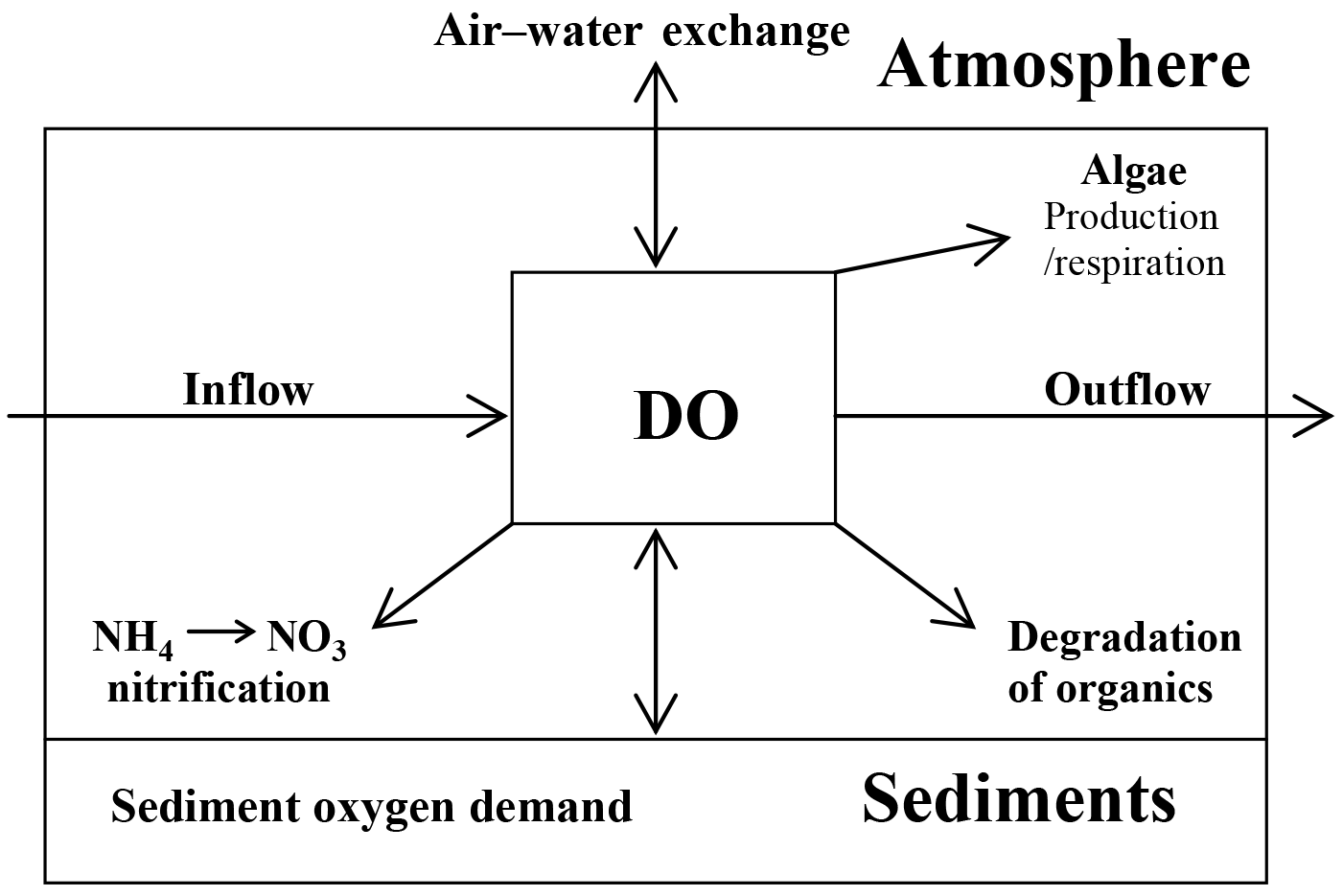
In CAEDYM, the algorithms that affect DO relate to air–water fluxes, sediment oxygen demand (SOD), microbial uptake during organic matter mineralization and nitrification, oxygen production, and respiration by primary producers (e.g., phytoplankton), and respiration by other optional biotic components (Hipsey et al., 2007). The air–water DO flux is calculated using the model of Wanninkhof (1992) and the flux equation of Riley and Skirrow (1974). SOD is represented by a function that varies the rate with overlying water temperature and DO concentration. Removal of DO occurs through microbial activity, including mineralization of organic matter and nitrification, as well as phytoplankton respiration. Figure 1 shows a schematic for the DO flux paths in CAEDYM.
2.3 Data collection
A water quality and meteorological monitoring buoy was installed in Lake Rotorua, New Zealand, near the deep central part (38∘04′32.7′′ S, 176∘16′01.88′′ E) in July 2007. Lake Rotorua is a shallow, eutrophic lake with an area of 80 km2 and mean depth of 10.8 m. The buoy transmits in near real-time data collected at 15 min intervals for a range of variables encompassing meteorology (wind speed and direction, air temperature, relative humidity, barometric pressure, precipitation) and water quality (surface and bottom DO concentration and percentage saturation, surface chlorophyll fluorescence, and water temperature at 2 m intervals over the 21 m water depth, where the buoy is located). The data are telemetered to an online database by GRPS modem. Shortwave solar radiation was measured at a weather station near the lake edge. All sensors were calibrated regularly for quality assurance. The quarter-hourly data were aggregated to hourly and daily time steps prior to analysis, in order to smooth some of the unexplained instantaneous anomalies that can sometimes occur with in situ optical instrumentation. In addition, total phosphorus and total nitrogen concentrations were measured monthly at two depths (1 and 19 m below surface) near the lake buoy station.
2.3.1 Autocalibration procedure for DYRESM-CAEDYM
The autocalibration model was implemented by following a number of steps. First, the modeler chooses a fixed simulation period when all the data required by the model were collected (i.e., the initial water quality data at the beginning of simulation, inflows, outflows, and meteorological data during the whole period). The time step was set to be 3600 s for the numerical integration in all simulations. Then all physical and biogeochemical parameters were fixed in their respective input files. When the model output was not sensitive to the parameter judged by experience or when fixed parameter values could be used (e.g., stoichiometric parameters), the minimum and maximum value were set to be equal and the parameter calibration was deemed unnecessary. A random search module was then run for all remaining parameters to produce files with combinations of parameters which could then be used to generate independent runs of the DYRESM hydrodynamic module. Simulations of water temperature extracted from the output file (DYsim.nc) were then compared with temperatures measured at corresponding depths and times. A physical parameter set was then chosen automatically based on minimizing the RMSE in comparisons between simulations and observations (Table 1). An alternative approach is to enter the physical parameters manually as many of these parameters can be fixed on the basis of their theoretically constrained values. We used a total of 10 000 iterations to choose the best fit of the physical parameter set. The DYRESM-CAEDYM model was then run with the selected physical parameters and a set of water quality parameters chosen from the MCS procedure with the same number of iterations. The RMSE was estimated for comparisons of simulations and observations for the variables chlorophyll a and DO. The combined RMSE is the sum of RMSEs for chlorophyll a and DO with each RMSE multiplied by an arbitrarily chosen weighing factor varying from 0 to 1. The four DYRESM-CAEDYM parameter files (par, bio, chm, and sed) were then chosen, which minimized the combined RMSE of these two variables with corresponding weighing factors.
2.3.2 Statistical evaluation methods for the autocalibrated model
The accuracy of the autocalibrated model was tested by RMSE, Nr, and Pearson correlation coefficient (r) as
where Oi is the measured value, Si is the simulated value, is the average of measured values, is the average of simulated values, and N is the total number of observations. Nr is known as the modeling efficiency and can be negative or positive. A positive value indicates that the simulations describe the trend of measurements better than the mean of observations and a negative value shows the opposite. The maximum value of Nr is 1.0, which means the model fits the observed values exactly. The subscript i for O and S represents the serial number of observations and simulations which are used for the statistical analysis. The objective of the autocalibration procedure was to minimize the RMSE values and maximize Nr and r values. One of these three parameters or a combined value of them can be chosen for obtaining the serial number of the iteration that produces the “best” simulation.
We used the period 13 July 2007–13 January 2009 (551 days) for model calibration and validated the calibrated model using data from the period 15 January 2009–8 June 2011 (875 days).
3.1 Physical parameter set selection
Table 1 shows the set of physical parameters that minimized the RMSE for temperature over the 10 000 model runs. A comparison of simulated and observed water temperature is shown in Fig. 2.
Table 1Selected physical parameters used in DYRESM based on autocalibration from 10 000 iterations.
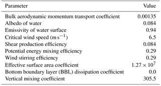
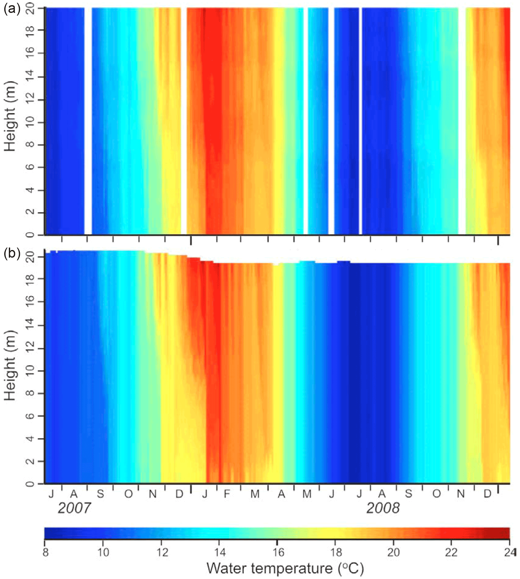
Figure 2Comparison of observed (a) and simulated (b) water column temperature based on daily data from 13 July 2007–13 January 2009. Height at the y axis represents the water height from the bottom.
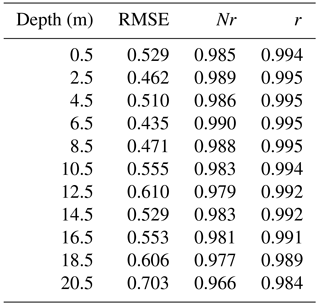
The water temperature simulations agreed well with observed values at all 11 observed depths (0.5 to 20.5 m at intervals of 2 m), and captured the dynamic nature of lake mixing, which in Lake Rotorua is characterized by occasional periods of stratification in which there are vertical temperature gradients interspersed with little or no temperature gradient when the lake is vertically mixed (Read et al., 2011). The Pearson correlation coefficient (r) between model output and measured temperature over all depths exceeded 0.98 with a RMSE of < 0.71 ∘C (Table 2). The RMSE was the lowest at a depth of 6.5 m (0.44 ∘C) of all of the observed depths, and the r value was also the greatest and Nr closest to 1.0 at this depth. The accuracy of simulations of bottom water temperature was not generally as accurate (in terms of RMSE, r, and Nr statistics) as for surface water temperature, but the ability of the model to capture the timing, frequency, and duration of stratification events (Fig. 2) was considered acceptable as a basis to carry out simulations of water quality by coupling DYRESM with CAEDYM.
Table 2Statistical results (RMSE, Nr, and r value) between simulations and observations of water temperature at different depths from 0.5 to 20.5 m at intervals of 2 m. The sample number is 436 for the bottom layer (depth 20.5 m) and 510 for all other layers.
3.2 Hypoxia simulation
3.2.1 Autocalibration
In CAEDYM, the most sensitive parameters in the DO simulation are the SOD and half saturation constant for DO consumption, DO production through phytoplankton photosynthesis and DO consumption through respiration of phytoplankton, mineralization of organic matter, nitrification, and denitrification. These processes are represented schematically in the CAEDYM configuration shown in Fig. 1. From a total of 10 000 simulations of the DYRESM-CAEDYM model with different input parameters it was possible to identify the parameter data set with the minimum value of RMSE to obtain the best match to observed values of DO. The values of the optimized parameters are shown in Table 3 and the hypoxia simulation results, represented by concentrations of DO, are shown in Fig. 3.
Table 3Values of key parameters for DO production and consumption in DYRESM-CAEDYM, chosen through autocalibration.
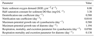
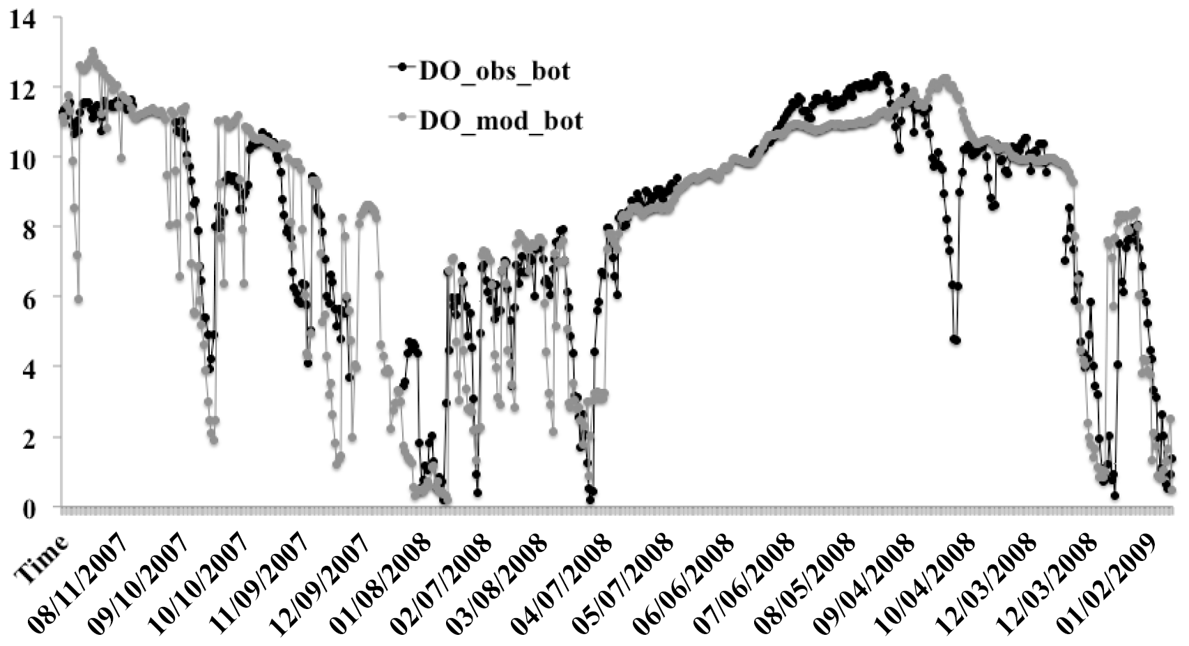
Figure 3Model autocalibration with comparison of daily bottom DO between simulations (DO_mod_bot, grey dots) and observations (DO_obs_bot, black dots) for depth of 20.5 m from 13 July 2007–13 January 2009 (551 days). The x axis represents time in the format of mm/dd/yyyy and the y axis represents DO concentrations (unit: mg L−1).
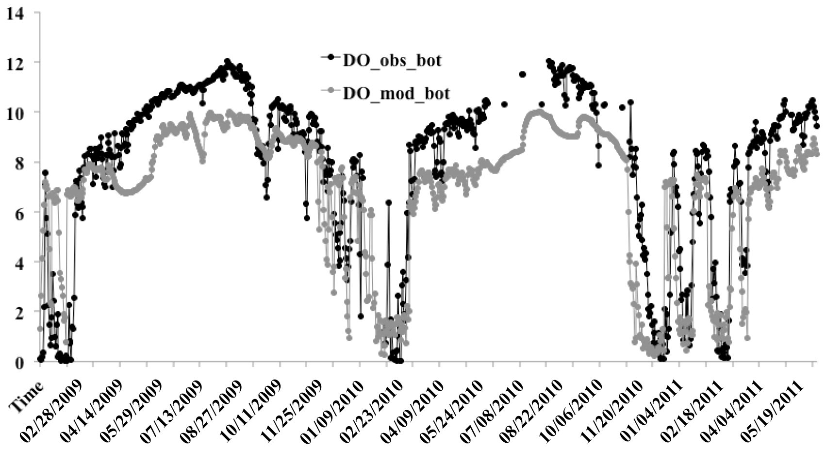
Figure 4Model verification with comparison of daily bottom DO between simulations (DO_mod_bot, grey dots) and observations (DO_obs_bot, black dots) at a depth of 20.5 m from 15 January 2009–8 June 2011 (875 days). The x axis represents time in the format of mm/dd/yyyy and the y axis represents DO concentrations (unit: mg L−1).
During the simulation period, there were five separate DO depletion events (DO < 4 mg L−1) observed in the bottom waters. The first occurred during 7 September–1 October 2007 with minimum DO of 3.95 mg L−1 (simulation 2.46 mg L−1) on 24 September (Julian day 267). The second and third events were observed in summer 2008, specifically 7 January 2008–10 February 2008 and 17 March–3 April 2008. The lowest DO (observation 0.21 mg L−1 and simulation 0.36 mg L−1) for the second event occurred on 18 January 2008 and for the third event on 31 March 2008 (0.19 mg L−1 and simulation 0.89 mg L−1). The fourth and fifth events were recorded in summer of 2009 with a minimum value of 0.72 mg L−1 (simulation 0.84 mg L−1) on 10 December 2008 and 0.5 mg L−1 (simulation 1.6 mg L−1) on 11 January 2009. All five bottom DO depletion events were captured with the DYRESM-CAEDYM model simulations, although the simulated trough (minima) of the first event was slightly below the observed values while all the other troughs exceeded the observations. Statistical tests to relate simulated and observed values over the entire simulation period gave a RMSE of 1.78 mg L−1, r of 0.87, and Nr of 0.75 (N=467). The simulations reflected the variation pattern of time serial measurements well with slightly oscillated gaps in winter and early autumn of 2008 (Julian day from 170 to 309). There was a small DO depletion event from 18 September 2008 (Julian day 262) to 3 October 2008 (Julian day 277), which was not captured by the model with the average value of DO (11.90 mg L−1) higher than the average observation value (8.40 mg L−1) by 3.5 mg L−1.
3.2.2 Model validation
The recorded bottom DO data from 15 January 2009 to 8 June 2011 (875 days) were used for model validation with the selected parameter set from the autocalibration process. The model captured all five hypoxic events with DO < 2 mg L−1 measured during 31 January 2009–21 February 2010, 12 February–25 March 2010, 2–24 December 2010, 9–17 January 2011, and 16 February–1 March 2011, with a RMSE of 2.07 mg L−1, Nr value of 0.62, and r value of 0.81 (N=738, Fig. 4). There was only one hypoxic event induced by intense stratification summer of 2009 and 2010, while three events were observed in the summer of 2011. In all cases, DO concentrations were < 0.7 mg L−1 during these events. The pattern of variation during these events was reproduced well by the model with the autocalibration parameter set although there were still minor differences between the absolute values for simulations and observations.
The DO capacity of water is greatly affected by temperature, but the distribution of DO in the water column is also strongly influenced by water column stratification, which in Lake Rotorua is controlled by variations in water density as water heats and cools. Therefore, to be able to accurately simulate the DO concentrations, it is necessary to choose a model of lake physical processes which accurately simulates water temperature dynamics, as shown with DYRESM model simulations in this study. The temperature profiles were well reproduced by the model, although there was water loss reflected by a water level decrease in the model by almost a half meter in January and February of 2008. The water loss probably resulted from the inflows/outflows boundary conditions which were induced by a catchment model.
Compared to the previous model parameter values reported by Burger et al. (2008), the value for water albedo yielded by the autocalibration was somewhat higher (0.084 compared to 0.07 in Burger et al., 2008), but water surface emissivity (0.94 in this work and 0.96 reported by Burger et al., 2008) was very similar. Thus our autocalibration procedure results in slightly less total solar energy received by the lake. Albedo at the water surface is one of the key parameters affecting the water heat budget in DYRESM. Nunez et al. (1972) found that on a daily basis, albedo ranged between 0.07 in early July to 0.11 in mid-November for Lake Ontario, North America, and that surface waves increase the value of direct-beam albedo, particularly at higher solar zenith angles. Albedo varies according to latitude and season, so some physical parameters may continue to require some flexibility in their values as long as there is not a complete process representation for them. There are five parameters related to vertical mixing in DYRESM: critical wind speed, potential energy mixing efficiency, shear production efficiency, wind stirring efficiency, and the vertical mixing coefficient. Their values, as selected by autocalibration, were 6.5 m s−1, 0.29, 0.084, 0.29, and 305.5, while they were given by Burger et al. (2008) as 4.0 m s−1, 0.25, 0.08, 0.6, and 400 based on trial-and-error calibration within the parameter limits (Yeates and Imberger, 2003). Statistical tests showed that RMSE values between simulated and observed water temperatures for the upper mixed layer (0.48 ∘C, 0–9 m) and the bottom layer (0.61 ∘C, 19.0 m) using our autocalibration approach were smaller than those reported by Burger et al. (2008) (0.97 ∘C for the surface-mixed layer and 0.88 ∘C for the bottom waters for a calibration period, and 0.86 ∘C and 0.67 ∘C, respectively, for the validation period). Therefore, autocalibration of DYRESM water temperature appears to be a useful tool to improve simulation accuracy for Lake Rotorua and potentially for other lakes.
Simulated bottom DO represented observations well in the calibration process, as it correctly captured the occurrence of five DO depletion events for bottom waters. One of the most sensitive parameters for DO simulations in bottom waters is SOD (g m−2 d−1). It varies as a function of the overlying water temperature and dissolved oxygen levels in CAEDYM but, as noted by Burger et al. (2008), it does not account for variations contributed by the dynamic nature of sediment composition (e.g., increased organic deposition following algal blooms). The SOD selected by autocalibration was 8.08 g m−2 d−1 in this study, which is greater than values selected for modeling a eutrophic estuary in Western Australia (6.0 g m−2 d−1; Robson and Hamilton, 2004), Tolo Harbour in Hong Kong (0.4–1.3 g m−2 d−1, Hu et al., 2001), shallow eutrophic Lake Alsdorf in Germany (1.5 g m−2 d−1, Strauss and Ratte, 2002), and Lake Onondaga in New York (1.68 g m−2 d−1, Gelda et al., 1995) but in the range of 0.34–9.02 g m−2 d−1 measured in the five southwestern lakes of USA by Veenstra and Nolen (1991). Sources of SOD may be divided into three basic categories: (1) microbial oxygen demand (bacteria, protozoa); (2) macrofaunal oxygen demand (primarily tubificid oligochaetes and insect larvae); and (3) chemical oxygen demand by inorganic oxidation of reduced chemical compounds (Finkelstein and McCall, 1981). Due to these varied influences, SOD can vary widely over time and space, both within and between lakes. For example, SOD in Lake Rotorua has been measured at values from 0.3 g m−2 d−1 (site 2, August 2003) to 4.0 g m−2 d−1 (site 3, November 2003, Burger et al., 2008). A value of 2.8 g m−2 d−1 was used for DO simulations with DYRESM-CAEDYM by Burger et al. (2008). In five southwestern US lakes (Broken Bow, Texoma, Birch, Pine Creek, and Pat Mayse) SOD ranged from 0.34 to 9.02 g m−2 d−1, after correction for temperature (Veenstra and Nolen, 1991). This parameter is mostly dependent on sediment components (i.e., organic matter, bacterial activity, and benthic fauna) and the overlying water environment (water temperature, underwater light, and vertical mixing), which will vary over seasons and locations in a specific lake.
Monte Carlo methods are generally preferred and more widely used for parameter estimation in environmental models than first-order variance propagation (Hession et al., 1996). Monte Carlo-based approaches continue to evolve and include BMC (Dilks et al., 1992; Bergin and Milford, 2000), MCMC (Gelfand and Smith, 1990; Gelfand et al., 1990; Zobitz et al., 2011), and GLUE techniques (Beven and Binley, 1992; Vrugt et al., 2009a, b). Among these methods, the Monte Carlo sampling is a general approach and assumes no structure associated with model error. It often serves as a screening approach to identify plausible regions of model parameter values (Stow et al., 2007). The BMC is based on MCS but with assumptions about model error structure to delimit plausible parameter regions (Stow et al., 2007). The main problem with this technique is that it does not converge toward the most probable region of the posterior distribution and can be extremely inefficient, rarely sampling from the most probable region (Qian et al., 2003). This problem is likely to be exacerbated when there are wide parameter ranges designated to include all possible values, but this may miss the important region of the posterior distribution in the Monte Carlo sample (Qian et al, 2003). GLUE is similar to BMC but permits a broader range of functions that define the model error structure (Stow et al., 2007). MCMC is specifically designed to sample from the posterior distribution in order to eliminate these problems and is regarded as one of the most efficient approaches for parameter sampling (Stow et al., 2007). It has been integrated into some autocalibration tools such as the shuffled complex evolution (SCE-UA, Duan et al., 1992, 1993), the shuffled complex evolution metropolis algorithm (SCEM-UA, Vrugt et al., 2003), and WinBUGS (Gilks et al., 1994). This method requires an appropriate algorithm dependent on the model form and a choice of distributional structure appropriate to represent the stochastic terms (Stow et al., 2007). A poor choice of the proposed distribution of parameters will result in slow convergence of the Markov chain (Vrugt et al., 2003).
Random Monte Carlo simulation, as adopted in our study, has the advantage of being easily incorporated into model code and programming, and can also include adequate consideration of “equifinality” of water quality models with large sets of parameters, without the need for the user to make assumptions regarding parameter distributions (as a simple uniform parameter distribution within the defined range is used). However, the success of parameter value selection is closely related to the user-defined upper and lower ranges of key parameters and the number of iterations performed. The number of simulations should be sufficiently large to reliably estimate the probability distribution of the output variables. Although a lot of hard disk space is required for saving stochastically produced parameter files, this is a progressively lesser concern due to the increased availability and reduced cost of storage space. An approach for reducing required hard drive space is to conduct a comparison between model outputs and measurements in terms of pre-defined statistical parameters for error evaluation after each model run, then sort all the iteration errors and save the parameter files with errors between simulations and observations that are smaller than an arbitrarily chosen threshold value of error. Sensitivity analysis might be an alternative option for reduction of required space for parameter file storage and to achieve an increase in model run-time speeds, since only the most sensitive parameters will be considered to change in the model autocalibration process.
Autocalibration tools have been widely used in watershed-runoff models but have had limited application to water quality models. This paper has detailed our prototype for an autocalibration tool for the widely used DYRESM-CAEDYM model. The success of its application is strongly dependent on prior knowledge about parameter value ranges and the number of iterations performed which is closely related to the computer's performance capability and the accuracy of observations, but has great potential to reduce the repetitive model iterations that are required using traditional trial-and-error calibration. Sub-modules for analysis of parameter sensitivity and model uncertainty could be included in further developments of the autocalibration approach in order to decide the most appropriate model parameters (on a case-by-case basis) to be used during calibration and thereby increase performance and reduce computation consumption.
-
MCS is an effective method for calibration of a dynamic water quality model with a massive number of parameters and equifinality to find an optimized parameter set in a complex environmental system, although it requires robust hardware.
-
For most of model users, the autocalibration software of DYRESM-CAEDYM developed in this paper is substantially less time-consuming and more efficient in parameter optimization than the conventional manual calibration procedure, which has been the standard tool practised for similar complex water quality models.
The code for the automatic calibration of DYRESM-CAEDYM is available within the Supplement.
The supplement related to this article is available online at: https://doi.org/10.5194/gmd-11-903-2018-supplement.
The authors declare that they have no conflict of interest.
The research was supported by National Natural Science Foundation of China
(NSFC) (41671205, 41661134036), NIGLAS 135 Strategic Planning Project (NIGLAS2017GH04), and
International Relationships Fund: New Zealand (MBIE)–China (MOST)
(2014DFG91780, UOWX1308). We also acknowledge support from Environment Bay of
Plenty.
Edited by: Sandra Arndt
Reviewed by: two anonymous referees
Alarcon, V. J., Johnson, D., McAnally, W. H., van der Zwagg, J., Irby, D., and Cartwright, J.: Nested hydrodynamic modelling of a coastal river applying dynamic-coupling, Water Resour. Manag., 28, 3227–3240, 2014.
Antenucci, J. P., Alexander, R., Romero, J. R., and Imberger, J.: Management stategies for eutrophic water supply reservior–San Roque, Argentina, Water Sci. Technol., 47, 149–155, 2003.
Arhonditsis, G. B., Adams-VanHarn, B. A., Nielsen, L., Stow, C. A., and Reckhow, K. H.: Evaluation of the current state of mechanistic aquatic biogeochemical modeling: citation analysis and future perspectives, Environ. Sci. Technol., 40, 6547–6554, 2006.
Asaeda, T., Pham, H. S., Nimal Priyantha, D. G., Manatunge, J., and Hocking, G. C.: Control of algal blooms in reservoirs with a curtain: a numerical analysis, Ecol. Eng., 16, 395–404, 2001.
Bergin, M. S. and Milford, J. B.: Application of Bayesian Monte Carlo analysis to a Lagrangian photochemical air quality model, Atmos. Environ., 34, 781–792, 2000.
Beven, K.: Prophesy, reality and uncertainty in distributed hydrological modelling, Adv. Water Resour., 16, 41–51, 1993.
Beven, K.: A manifesto for the equifinality thesis, J. Hydrol., 320, 18–36, 2006.
Beven, K.: Comment on “Equifinality of formal (DREAM) and informal (GLUE) Bayesian approaches in hydrologic modeling?” by: Jasper A. Vrugt, Cajo J. F. ter Braak, Hoshin V. Gupta and Bruce A. Robinson, Stoch. Environ. Res. Risk Assess., 23, 1059–1060, 2009.
Beven, K. and Binley A.: The future of distributed models: model calibration and uncertainty prediction, Hydrol. Process., 6, 279–298, 1992.
Beven, K. and Freer, J.: Equifinality, data assimilation, and uncertainty estimation in mechanistic modelling of complex environmental systems using the GLUE methodology, J. Hydrol., 249, 11–29, 2001.
Burger, D. F., Hamilton, D. P., and Pilditch, C. A.: Modelling the relative importance of internal and external nutrient loads on water column nutrient concentrations and phytoplankton biomass in a shallow polymictic lake, Ecol. Modell., 211, 411–423, 2008.
Chung, E. G., Bombardelli, F. A, and Schladow, S. G.: Modeling linkages between sediment resuspenstion and water quality in a shallow, eutrophic, wind-exposed lake, Ecol. Modell., 220, 1251–1265, 2009.
Chung, S. W., Imberger, J., Hipsey, M. R., and Lee, H. S.: The influence of physical and physiological processes on the spatial heterogeneity of a Microcystis bloom in a stratified reservoir, Ecol. Modell., 289, 133–149, 2014.
Copetti, D., Tartari, G., Morabito, G., Oggioni, A., Legnani, E., and Imberger, J.: A biogeochemical model of Lake Pusiano (North Italy) and its use in the predictability of phytoplankton blooms: first preliminary results, J. Limnol., 65, 59–64, 2006.
Cox, B. A.: A review of currently available in-stream water-quality models and their applicability for simulating dissolved oxygen in lowland rivers, Sci. Total Environ., 314–316, 335–377, 2003.
Cui, Y., Zhu, G., Li, H., Luo, L., Cheng, X., Jin, Y., and Trolle, D.: Modeling the response of phytoplankton to reduced external nutrient load in a subtropical Chinese reservoir using DYRESM-CAEDYM, Lake Reserv. Manag., 32, 146–157, 2016.
Dilks, D. W., Canale, R. P., and Meier, P. G.: Development of Bayesian Monte-Carlo techniques for water-quality model uncertainty, Ecol. Modell., 62, 149–162, 1992.
Duan, Q., Gupta, V. K., and Sorooshian, S.: Effective and efficient global optimization for conceptual rainfall-runoff models, Water Resour. Res., 28, 1015–1031, 1992.
Duan, Q., Gupta, V. K., and Sorooshian, S.: A shuffled complex evolution approach for effective and efficient global minimization, J. Optim Theory Appl., 76, 501–521, 1993.
Elliott, J. A.: Is the future blue-green? A review of the current model predictions of how climate change could affect pelagic freshwater cyanobacteria, Water Res., 46, 1364–1371, 2012.
Fekete, B. M., Wollheim, W. M., Wisser, D., and Vörösmarty, C. J.: Next generation framework for aquatic modeling of the Earth System, Geosci. Model Dev. Discuss., 2, 279–307, https://doi.org/10.5194/gmdd-2-279-2009, 2009.
Finkelstein, R. and McCall, P. L.: Some components of sediment oxygen demand in Lake Erie sediments, Project Completion Report No. 714436, Ohio State University, Water Resources Centre, USA, 1981.
Gal, G., Makler-Pick, V., and Shachar, N.: Dealing with uncertainty in ecosystem model scenarios: Application of the single-model ensemble approach, Environ. Modell. Softw., 61, 360–370, 2014.
Gan, T. Y. and Biftu, G. F.: Automatic calibration of conceptual rainfall-runoff models: optimization algorithms, catchment conditions, and model structure, Water Resour. Res., 32, 3512–3524, 1996.
Gelda, R. K., Auer, M. T., and Effler, S. W.: Determination of sediment oxygen demand by direct measurement and by inference from reduced species accumulation, Mar. Freshw. Res., 46, 81–88, 1995.
Gelfand, A. E. and Smith, A. F. M.: Sampling-based approaches to calculating marginal densities, J. Am. Stat. Assoc., 85, 398–409, 1990.
Gelfand, A. E., Hills, S. E., Racin-poon, A., and Smith, A. F. M.: Illustration of Bayesian inference in normal data models using Gibbs sampling, J. Am. Stat. Assoc. 85, 972–985, 1990.
Gilks, W. R., Thomas, A., and Spiegelhalter, D. J.: A language and program for complex Bayesian modelling, Statistician, 43, 169–177, 1994.
Green, C. H. and van Griensven A.: Autocalibration in hydrologic modelling: using SWAT2005 in small-scale watersheds, Environ. Modell. Softw., 23, 422–434, 2008.
Hamilton, D. P.: Numerical modelling and lake management: Applications of the DYRESM model, in: Theoretical Reservoir Ecology and its Applications, edited by: Tundisi, J. G. and Straškraba, M., Backhuys Publ., the Netherlands, 153–174, 1999.
Hamilton, D. P. and Schladow, S. G.: Controlling the indirect effects of flow diversions on water quality in an Australian reservoir, Environ. Int., 21, 583–590, 1995.
Hamilton, D. P. and Schladow, S. G.: Prediction of water quality in lakes and reservoirs, Part I – Model description, Ecol. Modell., 96, 91–110, 1997.
Han, B., Armengol, J., Garcia, J. C., Comerma, M., Roura, M., Dolz, J., and Straskraba, M.: The thermal structure of Sau Reservoir (NE: Spain): a simulation approach, Ecol. Modell., 125, 109–122, 2000.
Heathman, G. C., Flanagan, D. C., Larose, M., and Zuercher, B. W.: Application of the soil and water assessment tool and annualized agricultural non-point source models in the St. Joseph River watershed, J. Soil Water Conserv., 63, 552–568, 2008.
Hession, W. C., Storm, D. E., and Hann, C. T.: Two-phase uncertainty analysis: an example using the universal soil loss equation, T. ASAE, 39, 1309–1319, 1996.
Hipsey, M. R., Antenucci, J. P., Romero, J. R., and Hamilton, D. P.: Computational aquatic ecosystem dynamics model: CAEDYM v3 (Science Manual), Centre for Water Research, University of Western Australia, 2007.
Hu, F., Bolding, K., Bruggeman, J., Jeppesen, E., Flindt, M. R., van Gerven, L., Janse, J. H., Janssen, A. B. G., Kuiper, J. J., Mooij, W. M., and Trolle, D.: FABM-PCLake – linking aquatic ecology with hydrodynamics, Geosci. Model Dev., 9, 2271–2278, https://doi.org/10.5194/gmd-9-2271-2016, 2016.
Hu, W. F., Lo, W., Chua, H., Sin, S. N., and Yu, P. H. F.: Nutrient release and sediment oxygen demand in a eutrophic land-locked embayment in Hong Kong, Environ. Int., 26, 369–375, 2001.
Jackson, L. J., Trebitz, A. S., and Conttingham, K. L.: An introduction to the practice of Ecological Modeling, Bioscience, 50, 694–706, 2000.
Jayakrishnan, R., Srinivasan, R., Santhic, C., and Arnold, J. G.: Advances in the application of the SWAT model for water resources management, Hydrol. Process., 19, 749–762, 2005.
Jorgensen, S. E.: State of the art of Ecological Modelling in limnology, Ecol. Modell., 78, 101–115, 1995.
Kannel, P. R., Lee, S., Kanel, S. R., Lee, Y., and Anh, K.: Application of QUAL2Kw for water quality modelling and dissolved oxygen control in the river Bagmati, Environ. Monit. Assess., 125, 201–207, 2007a.
Kannel, P. R., Lee, S., Lee, Y. S., Kanel, S. R., and Pelletier, G. L.: Application of automated QUAL2Kw for water quality modelling and management in the Bagmati River, Nepal, Ecol. Modell., 202, 503–517, 2007b.
Kim, T. and Sheng, Y. P.: Estimation of water quality model parameters, KSCE J. Civ. Eng., 14, 421–437, 2010.
Krajewski, W. F., Lakshimi, V., Georgakakos, K. P., and Jain, S. J.: A Monte Carlo study of rainfall sampling effect on a distributed catchment model, Water Resour. Res., 27, 119–128, 1991.
Li, Y., Tang, C., Wang, C., Anim, D. O., Yu, Z., and Acharya, K.: Improved Yangtze River diversions: are they helping to solve algal bloom problems in Lake Taihu, China, Ecol. Eng., 51, 104–116, 2013a.
Li, X., Wang, C., Fan, W., and Lv, X.: Optimization of the spatiotemporal parameters in a dynamical marine ecosystem model based on the adjoint assimilation, Math. Probl. Eng., 2013, 1–12, 2013b.
Liang, S., Han, S., and Sun, Z.: Parameter optimization method for the water, quality dynamic model based on data-driven theory, Mar. Pollut. Bull., 98, 137–147, 2015.
Liu, Y.: Automatic calibration of a rainfall–runoff model using a fast and elitist multi-objective particle swarm algorithm, Expert. Syst. Appl., 36, 9533–9538, 2009.
Madsen, H.: Automatic calibration of a conceptual rainfall-runoff model using multiple objectives, J. Hydrol., 235, 276–288, 2000.
Makler-Pick, V., Gal, G., Gorfine, M., Hipsey, M. R., and Carmel, Y.: Sensitivity analysis for complex ecological models – A new approach, Environ. Modell. Softw., 26, 124–134, 2011.
Marsili-Libelli, S. and Giusti, E.: Water quality modelling for small river basins, Environ. Modell. Softw., 23, 451–463, 2008.
Mosley, L. M., Daly, R., Palmer, D., Yeates, P., Dallimore, C., Biswas, T., and Simpson, S. L.: Predictive modelling of pH and dissolved metal concentrations and speciation following mixing of acid drainage with river water, Appl. Geochem., 59, 1–10, 2015.
Ng, A. W. M. and Perera, B. J. C.: Selection of genetic algorithm operators for river water quality model calibration, Eng. Appl. Artif. Intell., 16, 529–541, 2003.
Nunez, M., Davies, J. A., and Robinson, P. J.: Surface albedo at a tower site in Lake Ontario, Bound.-Lay. Meteorol., 3, 1573–1472, 1972.
Pelletier, G. J., Chapra, S. C., and Tao, H.: QUAL2Kw – a framework for modelling water quality in streams and rivers using a genetic algorithm for calibration, Environ. Modell. Softw., 21, 419–425, 2006.
Pierson, D. C, Samal, N. R., Owens, E. M., Schneiderman, E. M., and Zion, M. S.: Changes in the timing of snowmelt and the seasonality of nutrient loading: can models simulate the impacts on freshwater trophic status?, Hydrol. Process., 27, 3083–3093, 2013.
Qian, S. S, Stow, C. A., and Borsuk, M. E.: On Monte Carlo methods for Bayesian inference, Ecol. Modell., 159, 269–277, 2003.
Read, J. S., Hamilton, D. P., Jones, I. D., Muraoka, K., Winslow, L. A., Kroiss, R., Wu, C. H., and Gaiser, E.: Derivation of lake mixing and stratification indices from high-resolution lake buoy data, Environ. Modell. Softw., 26, 1325–1336, 2011.
Refsgaard, J. C., van der Sluijs, J. P., Hojberg, A. L., and Vanrolleghem, P. A.: Uncertainty in the environmental modelling process – a framework and guidance, Environ. Modell. Softw., 22, 1543–1556, 2007.
Riley, J. P. and Skirrow, G.: Chemical Oceanography, Academic Press, London, 1974.
Robson, B. J. and Hamilton, D. P.: Three-dimensional modelling of a Microcystis bloom event in the Swan River estuary, Western Australia, Ecol. Modell., 174, 203–222, 2004.
Romero, J. R., Antenucci, J. P., and Imberger, J.: One- and three-dimensional biogeochemical simulations of two differing reservoirs, Ecol. Modell., 174, 143–160, 2004.
Rose, K. A., Megrey, B. A., Werner, F. E., and Ware, D. M.: Calibration of the NEMURO nutrient-phytoplankton-zooplankton food web model to a coastal ecosystem: Evaluation of an automated calibration approach, Ecol. Modell., 202, 38–51, 2007.
Santhi, C., Arnold, J. G., Williams, J. R., Dugas, W. A., and Hauck, L. M.: Application of a watershed model to evaluate management effects on point and nonpoint pollution, T. ASAE, 44, 1559–1770, 2001.
Schmolke, A., Thorbek, P., DeAngelis, D. L., and Grimm, V.: Ecological models supporting environmental decision making: a strategy for the future, Trends Ecol. Evol., 25, 479–486, 2010.
Seppelt, R. and Voinov, A.: Optimization methodology for land use patters using spatially explicit landscape models, Ecol. Modell., 151, 125–142, 2002.
Solomatine, D. P.: Genetic and other global optimization algorithms–comparison and use in calibration problems, Proc. 3rd International Conference on Hydroinformatics, Copenhagen, Denmark, 1021–1028, 1998.
Solomatine, D. P., Dibike, Y. B., and Nukuric, N.: Automatic calibration of groundwater models using global optimization techniques, Hydrol. Sci. J., 44, 879–894, 1999.
Stow, C. A., Reckhow, K. H., Qian, S. S., and Conrad, E.: Approaches to estimate water quality model parameter uncertainty for adaptive TMDL implementation, J. Am. Water Resour. Assoc., 43, 1499–1507, 2007.
Strauss, T. and Ratte, H. T.: Modelling the vertical variation of temperature and dissolved oxygen in a shallow, eutrophic pond as a tool for analysis of the internal phosphorus fluxes, Verh. Internat. Verein. Limnol., 28, 1–4, 2002.
Tanentzap, A. J., Yan, N. D., Keller, B., Girard, R., Heneberry, J., Gunn, J. M., Hamilton, D. P., and Taylor, P. A.: Cooling lakes while the world warms: effects of forest regrowth and increased dissolved organic matter on the thermal regime of a temperate, urban lake, Limnol. Oceanogr., 53, 404–410, 2008.
Takkouk, S. and Casamitjana, X.: Application of the DYRESM–CAEDYM model to the Sau Reservoir situated in Catalonia, Spain, Desalination Water Treat., 57, 12453–12466, 2016.
Tang, C., Li, Y., Jiang, P., Yu, Z., and Acharya, K.: A couple modelling approach to predict water quality in Lake Taihu, China: linkage to climate change projections, J. Freshw. Ecol., 30, 59–73, 2015.
Trolle, D., Jorgensen, T. B., and Jeppesen, E.: Predicting the effects of reduced external nitrogen loading on the nitrogen dynamics and ecological state of deep Lake Ravn, Denmark, using the DYRESM-CAEDYM model, Limnologica 38, 220–232, 2008a.
Trolle, D., Skovgaard, H., and Jeppesen, E.: The water framework directive: setting the phosphorus loading target for a deep lake in Denmark using the 1D lake ecosystem model DYRESM-CAEDYM, Ecol. Modell., 219, 138–152, 2008b.
Van der Perk, M. and Bierkens, M. F. P.: The identifiability of parameters in a water quality model of the Biebrza River, Poland, J. Hydrol., 200, 307–322, 1997.
Van Griensven, A. and Bauwens, W.: Multiobjective autocalibration for semidistributed water quality models, Water Resour. Res., 39, 1348–1356, 2003.
Van Griensven, A., Francos, A., and Bauwens, W.: Sensitivity analysis and auto-calibration of an integral dynamic model for river water quality, Water Sci. Technol., 45, 325–332, 2002.
Veenstra, J. N. and Nolen, S.L.: In-situ sediment oxygen demand in five southwestern U.S. lakes, Water Res., 25, 351–354, 1991.
Vilhena, L. C., Hillmer, I., and Imberger, J.: The role of climate change in the occurrence of algal blooms: Lake Burragorang, Australia, Limnol. Oceanogr., 55, 1188–1200, 2010.
Vrugt, J. A., Gupta, H. V., Bouten, W., and Sorooshian, S.: A shuffled complex evolution metropolis algorithm for optimization and uncertainty assessment of hydrologic model parameters, Water Resour. Res., 39, 1201–1214, 2003.
Vrugt, J. A., ter Braak, C. J. F., Gupta, H. V., and Robinson, B. A.: Equifinality of formal (DREAM) and informal (GLUE) Bayesian approaches in hydrological modeling?, Stoch. Environ. Res. Risk Assess., 23, 1011–1026, 2009a.
Vrugt, J. A., ter Braak, C. J. F., Gupta, H. V., and Robinson, B. A.: Response to comment by Keith Beven on “Equifinality of formal (DREAM) and informal (GLUE) Bayesian approaches in hydrologic modeling?”, Stoch. Environ. Res. Risk Assess., 23, 1061–1062, 2009b.
Wanninkhof, R.: Relationship between windspeed and gas exchange over the ocean, J. Geophys. Res.-Oceans, 97, 7373–7382, 1992.
Whitehead, P. G., Wilby, R. L., Battarbee, R. W., Kernan, M., and Wade, A. J.: A review of the potential impacts of climate change on surface water quality, Hydrolog. Sci. J., 54, 101–123, 2009.
Wu, Y., Liu, S., Li, Z., Dahal, D., Young, C. J., Schmidt, G. L., Liu, J., Davis, B., Sohl, T. L., Werner, J. M., and Oeding, J.: Development of a generic auto-calibration package for regional ecological modeling and application in the Central Plains of the United States, Ecol. Inform., 19, 35–46, 2014.
Yeates, P. S. and Imberger, J.: Pseudo two-dimensional simulations of internal and boundary fluxes in stratified lakes and reservoirs, Int. J. River Basin Manage., 1, 297–319, 2003.
Zhang, L., Xu, M., Huang, M., and Yu, G.: Reducing impacts of systematic errors in the observation data on inversing ecosystem model parameters using different normalization methods, Biogeosciences Discuss., 6, 10447–10477, https://doi.org/10.5194/bgd-6-10447-2009, 2009.
Zobitz, J. M., Desai, A. R., Moore, D. J. P., and Chadwick, M. A.: A primer for data assimilation with ecological models using Markov Chain Monte Carlo (MCMC), Oecologia, 167, 599–611, 2011.