the Creative Commons Attribution 4.0 License.
the Creative Commons Attribution 4.0 License.
 | 12 Dec 2018
OLYMPUS v1.0: development of an integrated air pollutant and GHG urban emissions model – methodology and calibration over greater Paris
Arthur Elessa Etuman
Isabelle Coll
Air pollutants and greenhouse gases have many effects on health, the economy, urban climate and atmospheric environment. At the city level, the transport and heating sectors contribute significantly to air pollution. In order to quantify the impact of urban policies on anthropogenic air pollutants, the main processes leading to emissions need to be understood: they principally include mobility for work and leisure as well as household behavior, themselves impacted by a variety of social parameters.
In this context, the OLYMPUS modeling platform has been designed for environmental decision support. It generates a synthetic population of individuals and defines the mobility of each individual in the city through an activity-based approach of travel demand. The model then spatializes road traffic by taking into account congestion on the road network. It also includes a module that estimates the energy demand of the territory by calculating the unit energy consumption of households and the commercial–institutional sector. Finally, the emissions associated with all the modeled activities are calculated using the COPERT emission factors for traffic and the European Environmental Agency (EEA) methodology for heating-related combustion. The comparison of emissions with AIRPARIF's regional inventory shows discrepancies that are consistent with differences in assumptions and input data, mainly in the sense of underestimation. The methodological choices and the potential ways of improvement, including the refinement of traffic congestion modeling and of the transport of goods, are discussed.
- Article
(8314 KB) - Full-text XML
- BibTeX
- EndNote


As the world's population grows, the share of the population living in urban areas also increases (United Nations, 2014). These areas can be described as hubs of activity with a substantial density of individuals, buildings, transport networks and employment centers. All the human activities associated with these metropolises induce a large local consumption of fossil energy and natural resources, favoring the concentration of a great variety of nuisances (noise, stress, pollution). Among the most emitting activities induced by the city, one can find – according to the IPCC nomenclature (IPCC, 1996) – energy consumption, industrial processes, the use of solvents and agriculture. However, at the city level, anthropogenic emissions are mainly the result of the combustion of road transportation fuels and residential, commercial and institutional heating and boiling, which account for more than half of total urban emissions (International Energy Agency, 2016). In Europe in particular, some cities are associated with the massive use of passenger cars (and sometimes even diesel fuel), which further increases their potential for the emission of air pollutants. In these areas, road transport and the production of electricity and heat represent more than 60 % of anthropogenic emissions of nitrogen oxides (NOx), particles smaller than 2.5 µm (PM2.5) and non-methane volatile organic compounds (NMVOCs) (International Energy Agency, 2016). Quantitatively, although sulfur oxide (SOx) emissions have declined since the 1990s, NOx and particulate matter (PM) emissions continue to increase in Asia and show no clear downward trend in Europe (Amann et al., 2013; Klimont et al., 2017; Miyazaki et al., 2017). As a result, even though exposure to short-lived peaks is decreasing, the exposure of the population to chronic pollution is still high in European urban areas (EEA, 2015), and 94 % of exceedances of the short-term limit value for PM10 have been observed in urban or suburban areas (EEA, 2016). Air pollution has serious consequences for human health. Recent estimates confirm the considerable burden of diseases associated with air pollution in urban areas, which results in pulmonary and cardiovascular diseases, cancer, certain types of diabetes in adults, and attacks on the neuronal development of very young populations (World Health Organization, 2013). From an economic perspective, it leads to high health care costs and to a significant drop in productivity for businesses. At the same time, societal questions related to the degradation of air quality arise. According to a survey carried out between 2007 and 2015 on behalf of the European Commission (European Commission, 2010), there are nine European Union capitals among the 20 cities with the lowest rate of people satisfied with the quality of the urban air, with the greatest decrease in the satisfaction index being observed in greater Paris.
Given the systemic nature of urban areas, it became clear that we could no longer ignore the links between urban morphology, individuals, energy consumption and pollutant emissions when dealing with environmental urban issues (Le Néchet, 2010) – urban morphology (or urban form) is defined here as the patterns of space occupation by a metropolis measured by the density and degree of hierarchization of the different urban cores. Indeed, the IPCC has recently recognized the impact of four variables linked with urban morphology (density, mixed land use, connectivity and accessibility) on energy consumption, climate and air quality issues. The effects of these four variables are expressed through the elasticity of the number of kilometers traveled, a parameter called “vehicle km traveled – VKT” (Seto et al., 2014). First, urban density, which reflects the spatial distribution of population, employment, housing or transport structures, impacts mobility choices through the deployment and sustainability of the local transport supply. Mixed land use (estimated by local employment-to-household ratios or household-to-services ratios, for example) also determines the morphology of the city, since a reduction in land use diversity reinforces the centrality of activities and shapes the population mobility for all trip purposes. Connectivity corresponds to the spatial structure and density of roads and pedestrian paths: in particular, it has been shown to promote walking. Finally, accessibility – defined as access to jobs, housing and services – can help reduce VKT, particularly for professional mobility (commuting). The way in which the urban form, the distribution of employment areas and the transport supply impose spatial interactions between individuals can be identified as the urban organization (Bretagnolle et al., 2010). Such an organization appears clearly dependent on the cost of energy. And when the relations between urban form and daily mobility are questioned, they invariably lead to classic issues in the literature (Melia et al., 2011; Le Néchet, 2010; Schindler and Caruso, 2014): spread urban forms would be the most energy-consuming structures, while a strong hierarchy between urban centers with an increase in central compactness would help reduce the distance to jobs and the use of a car. Moreover, dense urban forms, unlike spread urban forms, allow for a more efficient use of energy through the use of dense networks (heating, electricity, gas). However, it seems that dense urban structures also tend to reduce the share of local trips undertaken by sustainable modes due to increased metropolitan integration.
Models that aim to predict air quality in a given geographic area (called chemistry transport models – CTMs – or air quality models – AQMs) require a set of input data that includes an anthropogenic emission inventory. This type of input characterizes the intensity, the composition, and the spatial and temporal distribution of pollutant releases by human activities. Emission inventories for a given situation can be obtained either through a top-down (using national aggregated information and indicators to spatialize the emissions) or a bottom-up (collecting local information from specific activities – e.g., road traffic count data – to generate a high-resolution inventory) process. Conventionally, regulatory abatement coefficients are applied to current emissions to produce prospective emission inventories and to account for both technological developments and the effects of a constant reevaluation of emission standards. The emission scenarios approach traditionally uses these modified inventories to simulate air quality over a given time horizon. However, considering the abovementioned findings, prospective emissions calculations need to be rethought to take into account all the parameters affecting the urban organization and produce a more comprehensive calculation of energy consumption in the urban area. In particular, the models providing prospective emission scenarios to AQMs should be able to predict the effects of urban planning and individual practices on mobility and energy demand. Only by integrating emission scenarios of this nature into air quality models can the levers of urban air quality and sustainability be identified. Finally, it is also important to go beyond the quantification of future pollutant emissions and the mapping of air quality obtained through AQMs and consider exposure to air pollution, which makes it possible to address the issues of environmental inequalities and health risks. Indeed, the relationship between the individual and urban space is known to be at the origin of a highly differentiated exposure, discriminating places of residence, lifestyle and social categories. But our understanding of this issue remains uncomplete, and additional research that integrates the theory and practice from both air pollution and social epidemiology is expected (O'Neill et al., 2003). In particular, it is essential to change the traditional calculations of exposure to integrate mobility within the urban space and take into account the evolution of the exposure of individuals during the day (Steinle et al., 2013).
There are still few research projects in the literature that have included a large number of urban components into emission scenarios dedicated to AQMs (Manins, 1995; Marquez and Smith, 1999; Martins, 2012; De Ridder et al., 2008). Prospective modeling research in the 2000s has revealed the determining role of mobility and city configuration (considered as the spatial organization of buildings, services and networks) in the exposure of individuals, but the study focused on academic situations (Borrego et al., 2006). However, over the last decade, social components have progressively been integrated into urban emissions models, such as TASHA-MATSIM-MOBILE6.2C (Hao et al., 2010) and TRANUS-TREM (Bandeira et al., 2011), which are now able to quantify the impact of urban policies on road traffic emissions through carpooling, transportation fleet technology and individual modal choice. The strength of these models is linked to the implementation of a microsimulation approach based on individual choice, which depends on economic parameters. However, most of the applications focused on road traffic emissions only (Hatzopoulou et al., 2008; Hülsmann et al., 2014), whereas in the current context that places particular emphasis on the emerging concept of sustainable cities, it is necessary to take into account all air pollutant emissions related to energy consumption, insofar as they interact with air quality and climate change. In particular, there is a need to also take into account small combustion emissions (both residential and commercial) and their related policies to go further in the realism of the urban scenarios and to address the issue of air quality levers in a more holistic manner.
OLYMPUS is an emission model designed to produce a new generation of emission scenarios for air quality models (AQMs) at the scale of an urban area. It aims to meet the need described above to produce emission scenarios that integrate the interactions between the geographical aspects of the city, its population, the organization of buildings and urban networks, in order to produce a more comprehensive environmental decision support. It has been developed to integrate into a platform of disciplinary urban models connected in series. The platform provides data on urban morphology, the localization of activity centers and the organization of transport networks corresponding to an urban planning scenario or more broadly to public policies. OLYMPUS uses these data to produce a transport and energy demand diagnosis in the study area, which takes into account the main parameters influencing the urban organization (urban morphology, population density, services and networks) based on the simulation of individual behaviors related to mobility and energy consumption. Finally, these diagnoses are used to produce a pollutant and greenhouse gas emission inventory corresponding to the simulated scenario and resulting from a systemic representation of urban areas that highlights the role of urban configuration, urban planning, individual choices and political forcing in the sustainability of cities. The use of this new-generation inventory in the CHIMERE air quality model (Menut et al., 2013), located at the end of the chain in our modeling platform, will make it possible to predict the air quality associated with the emission scenario produced by OLYMPUS and to provide a new form of decision support on the relationship between urban forms, population and air quality. In addition, OLYMPUS simulates the individual mobility data that will be needed to improve the calculation of population exposure to pollutants in the final stages of the modeling platform. After the air quality simulation, individual urban travels provided by OLYMPUS will be processed with the AQM-simulated concentration fields in order to create a space–time exposure budget for all individuals. Although this is beyond the scope of this article, improvement of exposure in our modeling platform is one of the great innovations brought by the development of the OLYMPUS model.
In this paper, the operation and main features of the OLYMPUS model are described. The different modules will be presented individually. An application to greater Paris will be presented in the last section. The model results for this case study will be presented, evaluated and discussed.
The main objective of the OLYMPUS model is to estimate the pollutant emissions resulting from energy-consuming activities at the scale of an urban system, considered as the area that groups the daily activities of its inhabitants and the buildings hosting them (Bretagnolle et al., 2010), to produce innovative emission scenarios for AQMs as part of environmental decision support. The first specific contribution of OLYMPUS is to process data from multiple disciplines, but dedicated to serving air quality modeling. The second specificity of OLYMPUS is to provide new forms of decision-making support for the environment, thanks to an emissions calculation approach that integrates individual behaviors. Indeed, OLYMPUS relies mainly on the decision of each agent of a synthetic population to estimate the modal share. It is thus able to take into account the possible “changes of practices” related to mobility. The same can be considered for domestic heating practices. Finally, the emission data produced by OLYMPUS allow us to build much more advanced emission scenarios than the air quality models have simulated so far (taking into account only a regulatory factor for emission abatement). From this point of view, OLYMPUS is a fairly comprehensive and innovative tool.
OLYMPUS is integrated into an urban modeling platform connecting in series several urban models. It has been designed to collect city-specific input data such as morphology, population distribution and employment centers, road transport networks and public transport, and climate variables that affect emissions. Climate data are provided by a meteorological model. In the current situation, land use, population and urban services can be obtained from surveys. When simulating a public policy scenario, these data can be provided by the outputs of the NEDUM-2D model (http://www.rgte.centre-cired.fr/Rubrique-de-services/Archive-Equipe/Vincent-Viguie/article/NEDUM-2D-model, last access: 24 October 2018) included in the platform and simulating an urban organization corresponding to an economic, environmental and urban planning scenario on a horizon given time. The first step in OLYMPUS is to simulate a synthetic population, its properties (such as age, type of household) and its spatial distribution in order to describe, count and then spatialize individual activities within the area. Then, OLYMPUS uses activity-based emission factors to produce a spatially based emission inventory for non-methane volatile organic compounds (NMVOCs), nitrogen oxides (NOx), carbon oxides (CO and CO2), SO2 and primary particles. The general structure of OLYMPUS is detailed below. At each stage of operation, the calculation methods will be precisely described.
2.1 Main characteristics
In its current version, OLYMPUS models the main pollutant emissions linked with energy consumption, namely road transport and combustion processes from domestic activities and building heating in the tertiary sector. This last sector is composed of activities related to trade and services, but also to information and communication as well as finance. It also includes public administration, education, human health and social action. It will also be referred to as the commercial–institutional sector. As shown in Fig. 1, OLYMPUS is composed of six calculation modules supporting four main tasks.
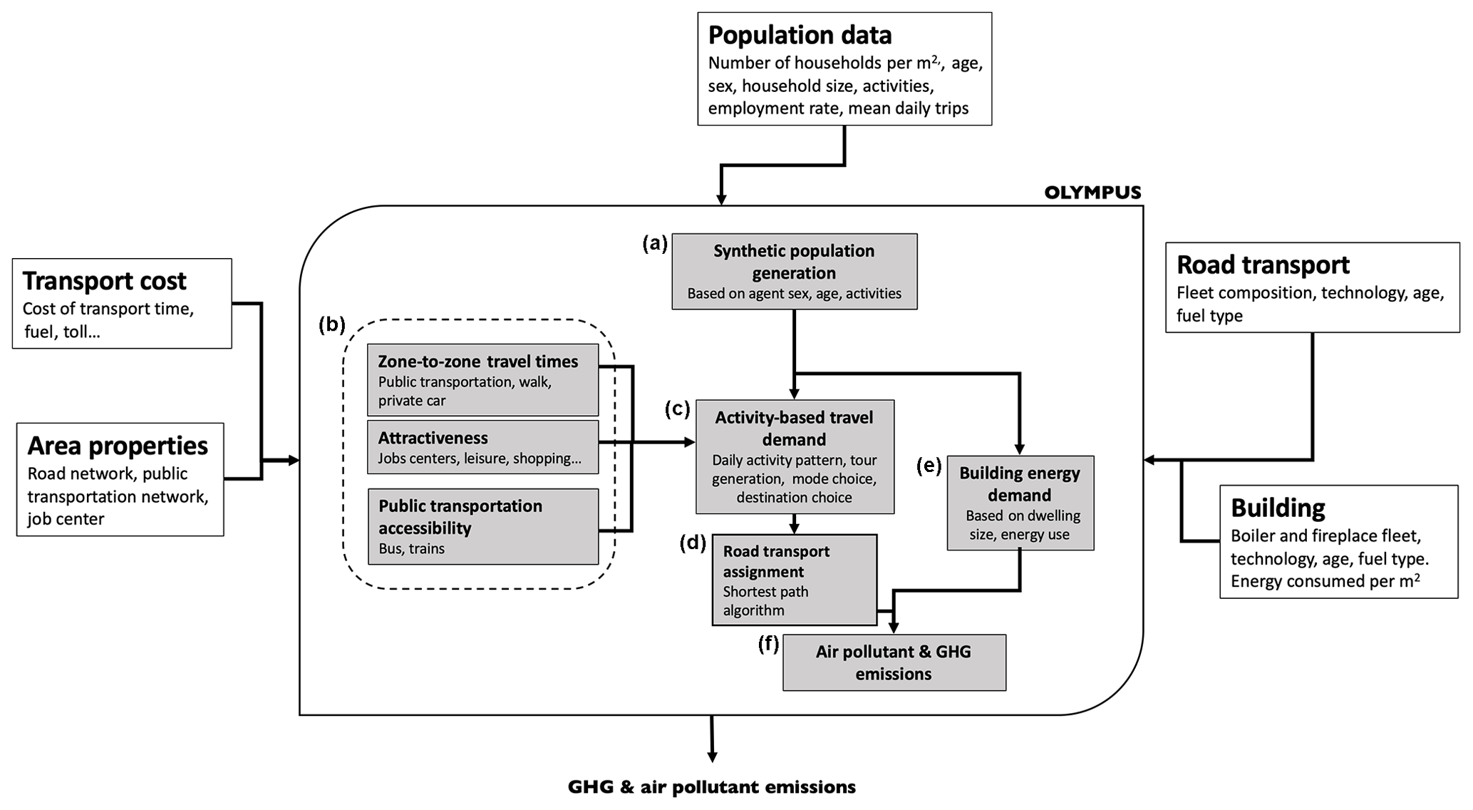
Figure 1Flowchart showing the OLYMPUS emissions operating system, as well as its main modules. (a) The synthetic population generation module (GAIA). (b) The generator of the transport time matrix, transportation accessibility indices and attractiveness of areas (THEMIS). (c) The transport demand module based on the activity of the synthetic population, and the modal choice in terms of transport (MOIRAI). (d) The module for assigning the travel demand on the road network (HERMES). (e) The module for the generation of energy demand at the regional level. (f) The module for the calculation of greenhouse gas and air pollutant emissions based on emission factors.
The first task of the model is to create a synthetic population to which a set of properties will be assigned. This synthetic population is designed to be representative of the population living in the territory concerned and is characterized by the age, gender and main activity of the agent as well as his or her belonging to a household. The creation of this synthetic population is based on the reconstitution of surveys in the GAIA module (panel a of the flowchart in Fig. 1).
The second task of OLYMPUS is to provide a transportation database built by taking into account the lifestyles of individuals. This database is obtained from successive diagnoses on the generation of individual trips – zonal attractiveness, spatial and temporal distribution of activities, transport supply, and choice of routes. In the OLYMPUS modeling process, this task is based on three modules.
-
A first module, THEMIS (b), defines the accessibility and attractiveness of the different administrative units of the city, as well as the average time travels between them.
-
An activity-based travel demand (ABTD) module called MOIRAI (c) computes the daily activity patterns of all agents. It also describes their daily mobility in time and space.
-
An assignment module called HERMES (d) provides spatialized daily trips by computing the shortest path between the origin and the destination of a trip (OD matrices).
In parallel, OLYMPUS is leading the third task of calculating the energy demand of buildings. To this end, the HESTIA (e) module calculates the average household energy consumption per square meter, the size of dwellings and the city energy mix in order to produce a spatialized energy demand for buildings, including a specific climatic correction on the simulated period.
In the fourth task, OLYMPUS generates emissions from both road transport and small combustion heating systems. These emissions are calculated using reference methodologies such as COPERT IV for road traffic, whose development was ensured by the European Environment Agency (EEA) in the framework of institutional and research activities on air quality and climate. For buildings, emission calculation methodologies are also taken from the EEA guidebook (European Environment Agency, 2013). The computation of pollutant emissions is carried out by the VULCAN module (f).
All running OLYMPUS scripts are shell based, Python 2.7 programmed, and C compiled for faster execution speed. For network graphs and spatialized data analysis, NetworkX (Hagberg et al., 2008), as well as GeoPandas and NetCDF, libraries were included in the Python interpreter. Due to the large number of computation loops, the model applies data parallelism that consists of partitioning the data with a multi-threading approach.
The GAIA synthetic population generator is the first OLYMPUS module to be run. It allows for the generation of a synthetic population representative of a given urban area. The synthetic population generator uses mainly urban census data to assign each agent in this population an age, gender and main activity, as well as socioeconomic parameters such as possession of a driver's license. The module distributes this synthetic population over the modeled territory through an urban zoning based on household densities in the urban area – an exogenous variable provided to the model. In the end, we obtain a synthetic population based on census data or demographic scenarios, with an individual description of its agents as the specific contribution of GAIA.
There are several statistical techniques for estimating the characteristics of a population in a restricted area, as reported in Rahman (2017). The most common method is the iterative proportional fitting (IPF) procedure (Deming and Stephan, 1940; Beckman et al., 1996; Müller and Axhausen, 2011), which generates an adjusted matrix of the survey data used to constrain the global synthetic population patterns based on the minimization of chi square, a method for estimating unobserved quantities from marginal numbers. The algorithm must be fed with the total population data and with subtotals for each of the property types using both aggregated and disaggregated data. Conditional probabilities are also part of the methodologies used to create a synthetic population. This approach is based on Bayesian statistics and relies on a representative sample of population, in which the discrete conditional probabilities governing every characteristic (e.g., age) are identified. Then, a unique value of this characteristic is assigned to each agent in the population using a random distribution that follows the identified probability law. This approach makes it possible to create (on the basis of a representative sample) a database that distinguishes each individual (disaggregated data) as well as each household and dwelling by assigning their own characteristics. These two methods differ in how to generate a built-in population but the results are recognized as quite comparable, although one of the main interests of the IPF procedure is its ability to generate greater variability than conditional probabilities in the population. Despite this, the use of the IPFP in a region such as the Île-de-France would require considerable work to structure the input data. For this reason, we decided to use the conditional probability approach, which has been widely used in the field of transport demand modeling (Antoni et al., 2010; Banos et al., 2010; Mathis et al., 2008). In order to mitigate a possible lack of variability, we implemented a spatial component in the distribution of the socioeconomic characteristics of agents.
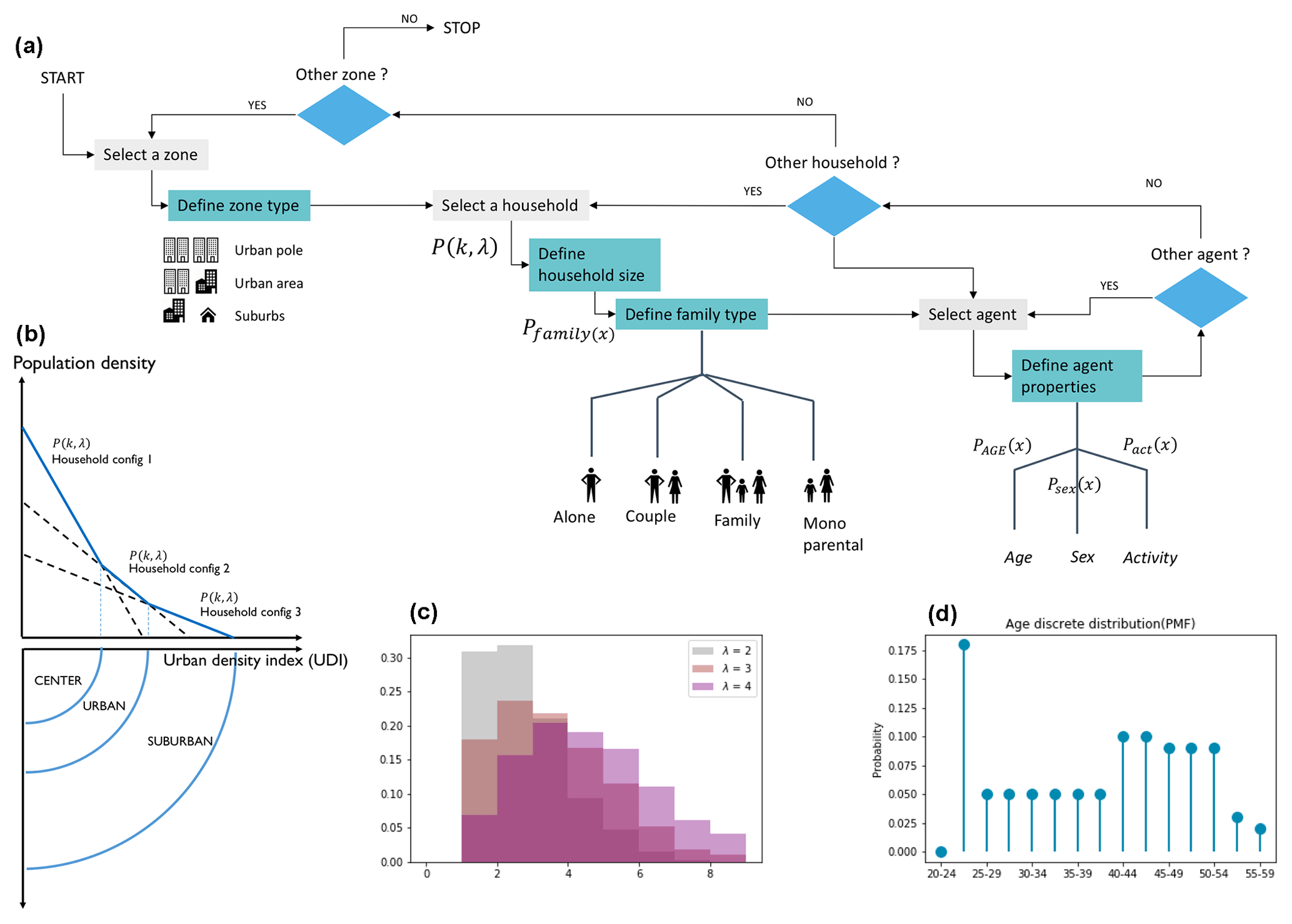
Figure 2(a) Synthetic population generator GAIA model operating flowchart. (b) Schematic representation of the urban density index (IDU). (c) Example of the household size probability distribution according to a truncated Poisson distribution. (d) Example of a representation of the distribution of the probability of mass function (PMF) of the age of an agent living alone.
The implementation of GAIA takes place in two main stages and is referenced in Fig. 2.
-
The determination of the urban structure is based on an urban density index (UDI) and divided into three classes: the urban pole (CENTER), the urban areas (URBAN) and the suburbs (SUBURBAN) (Fig. 2b).
-
For each household in the urban area, the module generates the synthetic population by defining the household size and the properties of the agent using conditional probabilities (Fig. 2).
3.1 Urban structure and population properties
The prerequisites for population generation are the definition of the domain and the classification of urban areas on the basis of an urban density index (UDI). GAIA discretizes the type of urban area on a scale of 1 to 3 (SUBURBAN – URBAN – CENTER) according to the population density.
The UDI is defined in Eq. (1). It is the result of the classification of the dataset into three large sets of urban density by applying a linear division of the domain from the sparsely populated areas to the very dense areas. It is based solely on real population density and the population is digitized according to the logarithm of population density.
where ∝1 and ∝2 are key classification values depending on the logarithm of household density, nhh is the number of households, z is a specific area of the domain and A is the surface area.
Figure 2b shows a schematic representation of the UDI as well as the population-specific attributes for each UDI value. Such discrimination of the properties is necessary for the realism of our output data because population density affects the urban landscape (buildings and houses), the location of activities and the structure of households. It is assumed here that the distribution of household types is different between urban centers, surrounding urban areas and suburbs (Pisman et al., 2011; Thomas et al., 2015) and that the distribution of buildings and single-family houses will vary between these different areas. Finally, we have added a variation in household structure with distance from the urban center according to Hulchanski (2010). These hypotheses offer greater variability in the spatial distribution of agents than a simple conditional probability distribution.
3.2 Generation of a synthetic population
The generation of the population depends on probability mass functions (PMFs) that rely on census data, as shown in Fig. 2d, which represent the age-specific PMF of an agent living alone. In each zone and for each household, GAIA uses a discrete probability distribution to
- a.
define the number of agents in the household,
- b.
characterize the type of family, and
- c.
define the gender, age and main activity of agents.
Equation (2) predicts the number of agents in the household according to the type of zone (CENTER, URBAN, SUBURBAN), which differ in the density of population and in the distribution of the types of housing. The probability of having n agents in the household is based on conditional probabilities and defined by a truncated Poisson distribution:
where λ is the average household size, n is the number of agents in the household and n∈A, with A= [1, 7] and A∈N. Figure 2c is an example of a household size probability distribution based on a truncated Poisson's law.
Equation (3) is used to define the type of household among the four family classes, which are as follows: single (male or female); couple – no children; couple with children; and single-parent family (male or female). The selection of the family type is also based on conditional probabilities (PFAM) and follows
where RnF is the family type defined for the n persons in the household
and P1F(n) and P2F(n) correspond to weighted functions based on survey data.
Equation (4) allows us to estimate the attributes of the agents (age, gender, main activity). The gender of each agent is defined by a conditional probability (while the gender of the partner is opposite), such as
where η represents the situation of the agent in the household, Rgdr is the sample space and consists of two elements {male, female}, Psex1() corresponds to a weighted function based on the census data and Psex2() is conditioned by the gender of the householder.
The age of an agent depends on the type of household, which is still based on conditional probabilities, and is linked to specific sample spaces: for householders, for couples (age difference less than 20 years) and for children. There are 20 age classes with a 5-year division.
where PA_1(n), PA_2(n) and PA_3(n) are probability mass functions based on census data. Rhouseholder, Rchild and Rpartner are age types defined for n people in the household with
The principal activity of the agent depends on age and the unemployment rate. Agents under 18 are educated and agents over 65 are retired. Other agents may be employed, unemployed or studying.
where Pact1(age) and Pact2(age) represent the mass probability functions giving the probability of having as a main activity one of the activities defined in Ract1 or Ract2.
To simulate the transportation demand according to the activities of the population, OLYMPUS requires a large number of external data. The spatial distribution of employment centers is a first key parameter: the calculation is based on a spatialized file containing the number of jobs per zone, usually in a geographic information system (GIS) format. To simulate ABTD, OLYMPUS uses socioeconomic data at a disaggregated level for each area, which this time can be provided by the GAIA synthetic population generator.
Transport networks are a second external parameter needed to calculate mobility. The road network includes urban and nonurban highways as well as major traffic lanes and information on no-load speeds. The public transport network includes all related stations, also in GIS format. All of these data will be analyzed at the finest accessible spatial scale, called the transport analysis zone (TAZ), which can be a district, a subdistrict, a municipality or any other division of the city. The resolution of the data foreshadows the refinement of the mobility of the population.
The modeling of urban road transport is organized in three stages:
-
determination of the attractiveness and accessibility of the different zones that make up the domain;
-
restitution of the agent travels on the basis of the realization of the programmed activities; and
-
assignment of motorized trips on the road network.
4.1 TAZ accessibility and attractiveness (THEMIS)
The operating diagram of THEMIS is presented in Fig. 3a. The main steps are
-
definition of accessibility and
-
computation of attractiveness.
One of the key forcing data of the ABTD model (ABTDM) is the accessibility of the TAZ, which provides the basis for mobility choices. Accessibility is calculated from all the activities considered useful for the agents within a given radius, its value also taking into account the public transport service in this area. For this purpose, THEMIS analyzes the population density, road network and public transport network of the TAZ. The result is an index with five levels of accessibility accounting for public and individual transport to the area and called the urban transport accessibility index (UTAI).
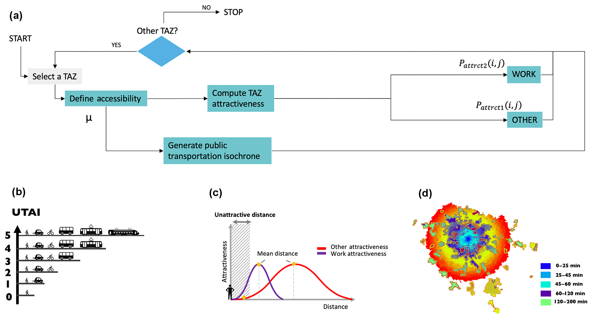
Figure 3(a) The transport time matrix generator, transportation accessibility indices in common and attractiveness of zones of displacements (THEMIS) flow diagram. (b) Schematic representation of UTAI. (c) Schematic representation of the attractiveness of an activity towards an individual as a function of distance. (d) Example of isochronous transit curves from the center of Paris.
This flag is used to set the access mode shares. As shown in Fig. 3b, an area with a UTAIMIN will only be accessible by walking (WALK), while an area characterized by a UTAIMAX will be well serviced with a wide choice of transport infrastructure. The definition of the five UTAI classes depends on the value of μ, defined by the following equation:
with
where and ∝4 are key classification values depending on the logarithm of household density and public transport density. nhh is the number of households per TAZ, nst is the number of public transportation stations in the TAZ and A is the area of the TAZ. The UTAI (see correspondence in Fig. 3b) thus helps to design the use of the city from its transport infrastructure and to define a realistic travel time for public transport, as represented on the isochronous curve of public transport in Paris (Fig. 3c).
The attractiveness of activities is an important parameter that shapes the agenda of agents. It can be defined as the ability of a zone to get an agent to carry out a given activity on the site, respecting the average length of the trip associated with this type of activity, as illustrated in Fig. 3c. The model assumes that there are two types of activities: WORK and OTHER. The complete list of OTHER activities taken into account in the ABTD model are the following.
-
HOME
-
SCHOOL
-
SHOPPING
-
SECONDARY
-
ACCOMPANYING
-
VISIT
-
LEISURE
The main parameter that differentiates our two types of activities is the average duration of the journey, which varies considerably, with the average distance traveled for commuting (home–work) being longer than that of other types of activities. The distance to the TAZ is an important variable in the estimation of its attractiveness for an agent. The attraction potential of WORK depends on the number of jobs in the TAZ. For OTHER activities, their attractiveness depends on the population density of TAZ. However, some activities like visiting a friend or going on vacation are still underestimated by the ABTD model. The computation of attractiveness is based on Huff's theory of the gravity model (Huff, 1964). It is based on the definition of an activity weight and works by analogy with Newton's law of gravity. The probability of conducting any activity at a specific location is therefore defined as follows:
where the attractiveness Ω is defined by
In this equation, dmean represents the average distance to reach the activity, while i and j are the indexes of the origin and destination zones, respectively.
In the end, the attractiveness parameter is highly dependent on the city's structure and the travel practices of the inhabitants. Kwan and Weber (2003) found that few people act to minimize their commute to work by relocating their home or workplaces. Given this, mobility surveys provided by some countries can be used to force average travel distances and make them more realistic.
4.2 Activity-based travel demand (MOIRAI)
The ABTD module MOIRAI simulates the mobility choices for each agent in the synthetic population during the day. One of the challenges of the module is to represent mobility in the most realistic way possible, taking into account the social constraints of each agent in space and time. Several ABTDMs exist in the literature. Malayath and Verma (2013) proposed a review of existing models and their uses. Based on this review, we decided to use random utility theory to simulate the choice of individuals in MOIRAI. In this theory, a stochastic approach makes it possible to take into account the rationality of agent decisions. That is, the decision is described as the choice of the agent to do what is most useful, depending on the opportunities available. In this process, utility is generally divided into two components, one describing the observed practices and the other describing the random component. In the theory of random utility, the main hypothesis on which the choice is based is that the maximization of utility influences the decisions of the agent. MOIRAI relies on the use of the multinomial logit (MNL) model (McFadden, 1973) in which the random components of utility are considered independent, identically distributed (IID) and follow a Gumbel distribution:
where Utilitymode,i represents the utility function of a transportation mode i.
MOIRAI is implemented in three main stages common to many ABTD models (Castiglione et al., 2015):
- 2.1
generate the daily activities of the agent (number of trips and tour sequence),
- 2.2
agent schedule management (duration of activities), and
- 2.3
identify the type of transportation used for each trip (location and modal choice).
These steps are described in the MOIRAI operating diagram in Fig. 4a.
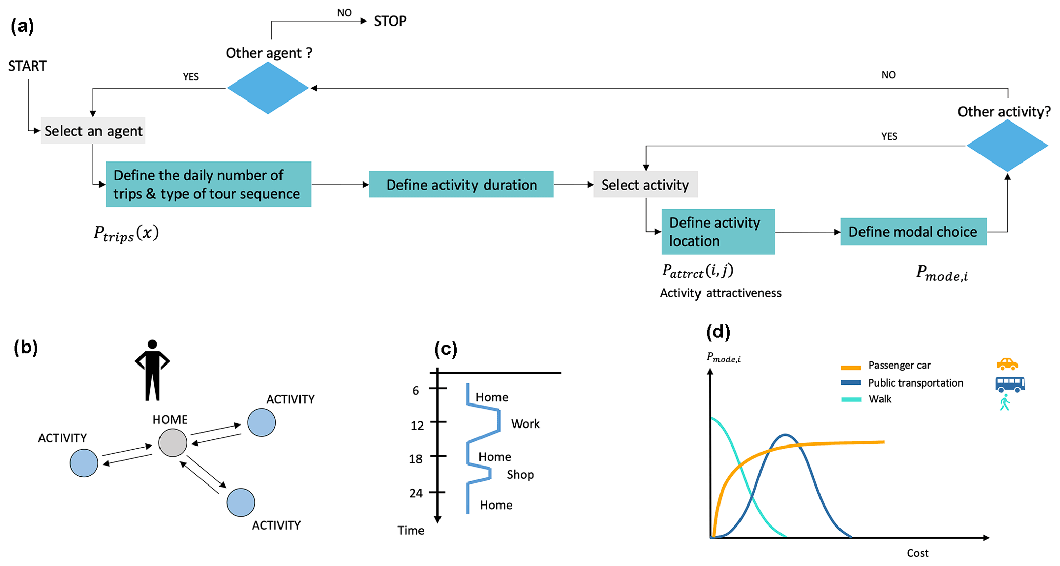
Figure 4(a) The transport demand module MOIRAI operating flow diagram. (b) Representation of a circuit of activities of an agent of the synthetic population. (c) Representation of the timetable of an agent of the synthetic population. (d) Representation of the probability of favoring a mode of transport according to the cost of transport time.
4.2.1 Generation of daily activities
An important step in modeling an agent's schedule is the estimation of the number of trips the agent makes during the day, as shown in Fig. 4b. A first step in the simulation of the agent's agenda is therefore to define priorities. The obligation to conduct an activity – such as going to work or accompanying children for care or education – defines the priority of an officer. Once these priorities are set, an agent can perform optional activities such as shopping, visiting a friend or going to the movies. There are three priorities in the model: work – school – accompanying (bring a child under 10 to school). The model can combine the priorities of the work and accompanying activities. The number of trips per day (p) performed by an agent depends on priorities (x) and is based on the following discrete probability distribution:
where Ptrips act1(x), Ptrips act2(x), Ptrips other(x) and Ptrips retired(x) represent the probability of performing p daily trips according to the x priorities of the agent and with .
The probability Ptrips(x) is derived from a specification of the number of trips per day based on age and priorities. This number of daily trips varies from country to country. It can be provided by local surveys or estimated from an aggregated survey database. We used information from household travel surveys, which indicates that the mobility of children and the elderly is lower than that of the population aged 20–60 years.
After determining the number of activities of the agent and establishing an order of priority, MOIRAI defines the sequence of trips. Sequences can start from home (home-based sequence, HBS), include multiple home returns (multiple home-based sequence, MHBS) or be fully performed without returning home (nonhome-based sequence, NHABS). Figure 5 shows the different types of sequencing modeled in OLYMPUS. Depending on the number of trips, it is possible to create a single home circuit or several circuits, one centered on the place of residence and others on the activities. The probability of making one or more circuits depends on the number of daily trips.
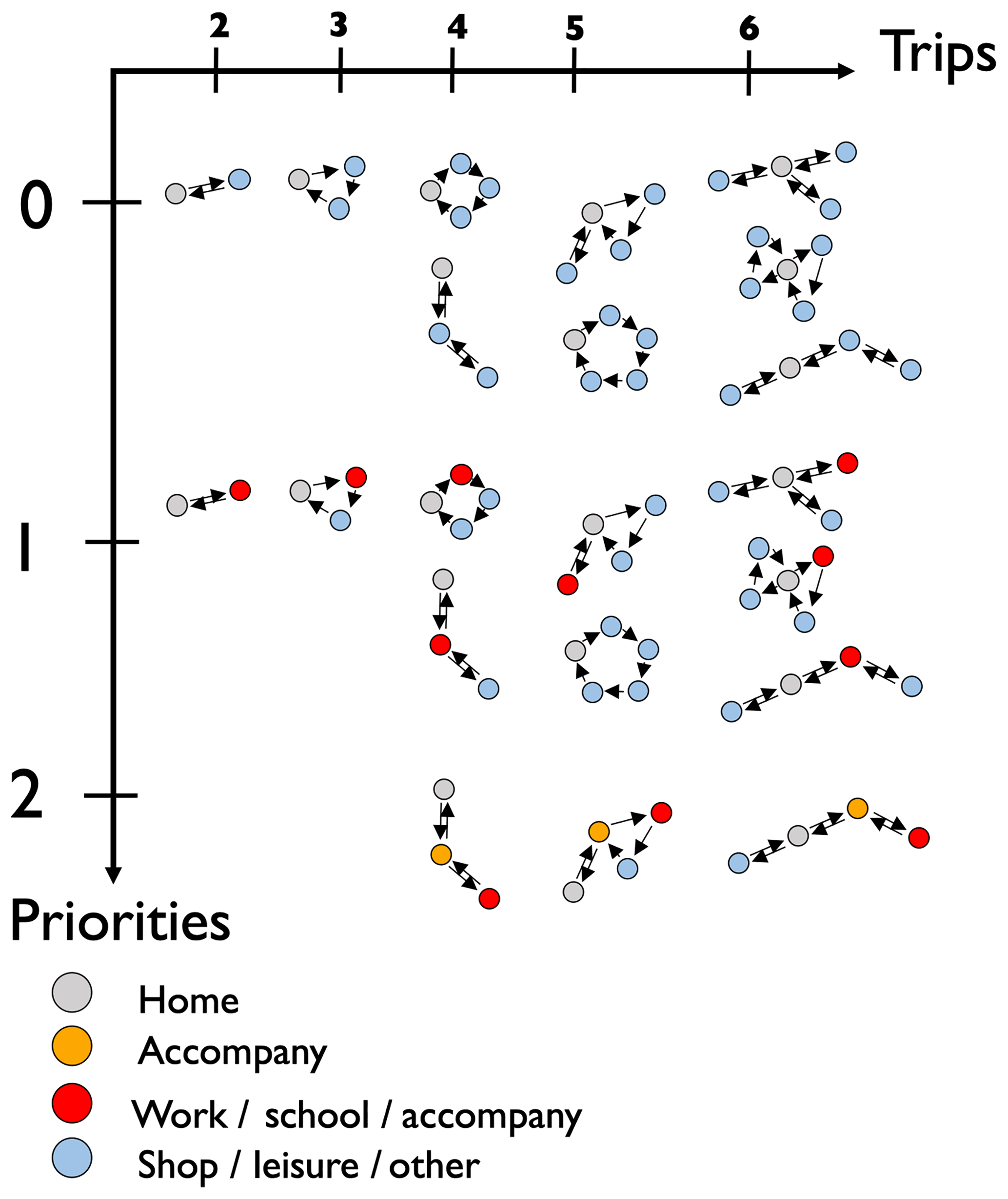
Figure 5The transport demand module MOIRAI activities circuit based on agent priorities and daily number of trips (p).
After generating the agent schedule, the module locates each activity. Depending on the TAZ in which the agent is located, the model estimates where the agent will have the highest probability of carrying out the planned activities. This is done according to the attractiveness of the TAZ calculated by THEMIS and by using Huff's random probability approach for choosing the place of activity. For the location of the WORK activity, we use the ΩP(i,j) probability of attractiveness of the employment center. For OTHER activities, the ΩP(i,j) probability of attractiveness is based on population density.
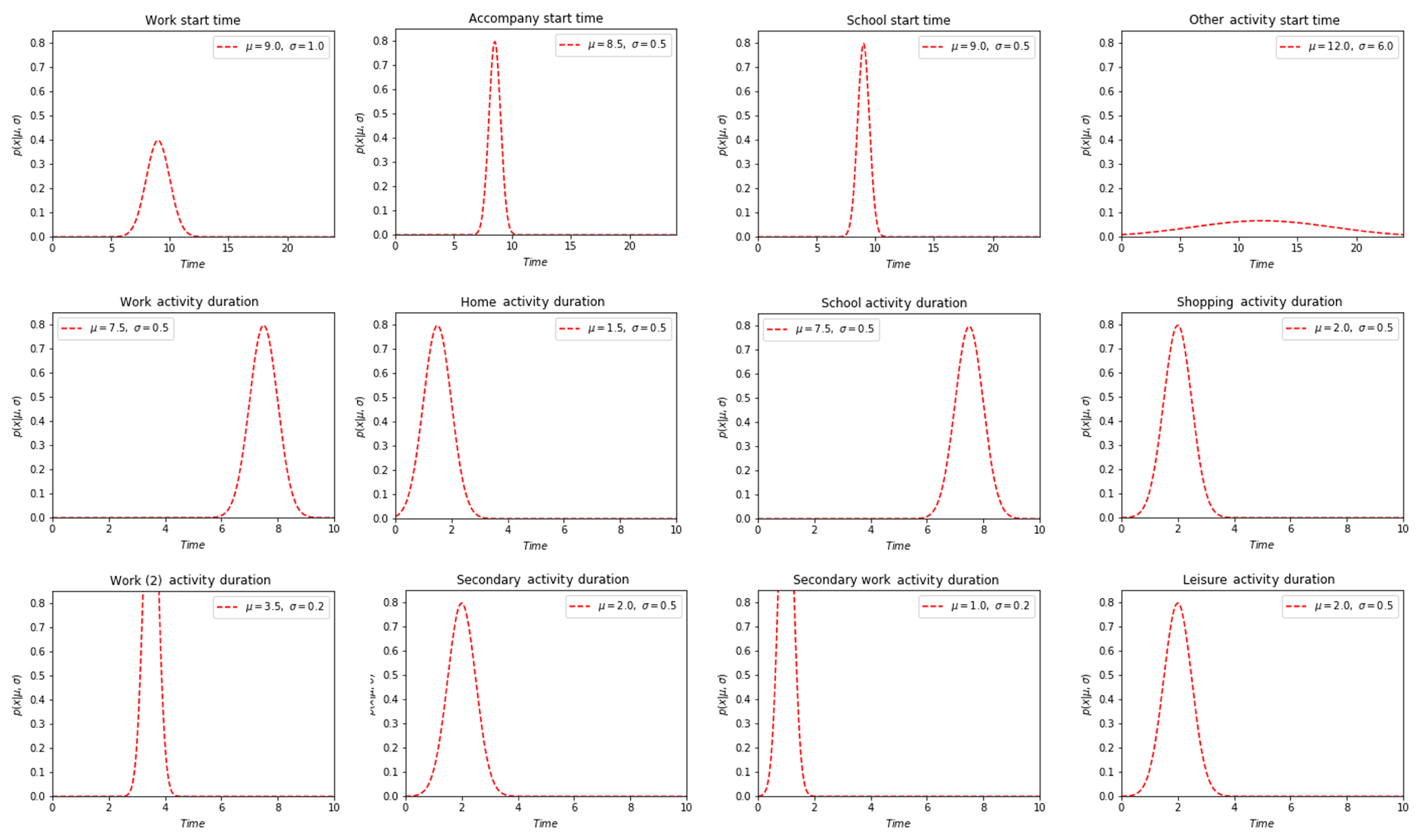
The last step in the generation of daily activities is the insertion of the time of realization of the activities, which requires the attribution of a duration to each of the actions carried out by the agent. As shown in Fig. 4c. MOIRAI calculates this parameter using conditional probabilities with a time step of 1 h. The module assigns a random value to the start time based on the agent's priorities. If the sum of the activities exceeds 24 h, the simulation is restarted.
For the first activity, the start time is calculated as follows:
where stescort(x), stschool(x), stwork(x) and stother(x) represent the start time of the first activity of the day. The start time is based on a normal distribution as shown in Fig. 6.
where
and Dur represent the duration of activities, defined as a random variable in a truncated interval over a time range. The distribution of start time and duration of activities in OLYMPUS is presented in Fig. 6.
4.2.2 Modal split
The modal choice is clearly a critical parameter for calculating pollutant emissions from urban mobility. In OLYMPUS, travel modes include WALK (walking and cycling), PC (passenger car and two-wheeled car) and PT (public transport including metro, bus, tram and train). The objective is to define the probability of using a specific mode of transport according to their utility for a given route and agent. The modal choice is obtained from the expression of the utility function for each transportation mode (Umod,i). The value of utility comes from a cost calculation including the generalized cost of transport (including the time budget (tbudget), the perception a of mode i and the monetary cost (mcost)). In this calculation, the travel time can be penalized by different elements of the trip such as tolls, congestion and parking problems included in the variable Pmod:
The utility function of the WALK mode mainly depends on the time cost of the trip. The WALK mode average speed, SpeedWALK mean, is defined to be 3.6 km h−1. Thus,
where PWALK represents walk penalties, and the distance between the origin and the destination activity, ODdistance, is based on the great-circle distance calculation,
where A and B respectively denote the origin and destination points, φA, φB, λA and λB represent their latitudes and longitudes, and dλ=λB–λA.
For the individual passenger car mode (PC), the utility function is defined as follows:
By default, the average speed of PC mode, SpeedPC mean, is set to 22.6 km h−1 in urban areas. This value is based on Hickman et al. (1999) and represents the average driving speed in urban areas recorded during the MEET project. The ODdistance is also based on the great-circle distance equation (Eq. 17).
The CostCAR variable represents the average kilometric cost of the use of a private car. All penalties are coded as additional monetary costs: these include tolls, parking tickets, congestion and taxes as well as additional penalties for short-distance trips. All of them can be summed in the calculation of PC mode utility. The time cost for the agent is calculated from the shortest path. This step of OLYMPUS requires considerable computation time because of the large number of agents.
With regard to the utility function of public transport (PT) from one TAZ to another, we use the following equation:
In this equation, the travel time with PT mode is TimePT. It depends both on the accessibility of the destination area and the average distance between origin and destination points. The average travel time from one TAZ to another includes the duration of walking, waiting and traveling. It is calculated using a linear regression based on time zone transport survey data and is therefore based on realistic values.
where αi,j represents the average transit time between two zones and a and b are the linear regression coefficients. WTime is the UTAI-dependent waiting time.
The tPT parameter is usually calculated using general transit feed specification (GTFS) data, if available for the city, and computed using either the connection scan algorithm (Dibbelt et al., 2013) or the RAPTOR algorithm (Delling et al., 2012). The limitation of these methods is the huge computing time required. As a consequence, they were not chosen here. Since public transport time is an essential variable for the estimation of the general cost of public transport, we have developed a methodology based on a zonal approach and using the UTAI. This method has limitations with respect to CSA or RAPTOR algorithms. However, we consider that a realistic simulation of the UTAI matrix and an appropriate calibration of the module with real transport times can lead to satisfactory results. The CostPT variable represents the daily cost of transit. Transit penalties may be well represented by the frequency of transit service.
4.3 Assignment
The transport demand previously generated by the ABTD module MOIRAI generates travel matrices providing information only about the origins and destinations of the flows. The next step is to project on our modeling grid the paths taken by the agents in order to provide spatialized pollutant emissions from transport. For this purpose, we only take into account flows related to private vehicle use.
There are three ways to handle traffic assignment. One is the microscopic approach, which manages the traffic at the scale of each vehicle, as proposed by models such as VISSIM (Gomes and May, 2004), AIMSUN (Barcelo et al., 1989) and PARAMICS (Cameron et al., 1994). A second approach is that of mesoscopic models, which are interested in the evolution of sets of vehicles, like the models CONTRAM (Taylor, 2003) and DYNASMART (Mahmassani et al., 2005). Both approaches are not very compatible with the scale of the city, on which we focus. Indeed, although the use of instant-emission models like PHEM (Rexeis et al., 2013) and MOVES (U.S. Environmental Protection Agency, 2013) can provide added value, obtaining input traffic data describing each cycle of acceleration and deceleration of the vehicle is quite difficult, and their consideration requires high computational time. These constraints make the microscopic approach somewhat precarious. We must therefore rely on a macroscopic description of the traffic in the form of a vehicle flow and using global variables such as the average speed on each section of a traffic axis, as in the DAVISUM (Broquereau, 1999) and TransCAD (Caliper Corporation, 2010) models. As most of these transport models are not open source, we opted for the development of our own traffic assignment model within the OLYMPUS ensemble: HERMES. HERMES is a macroscopic traffic module that works with average speed values for vehicle flows, ignoring the dynamics of traffic on a road. This approach is compatible with our simulation scale. It is also compatible with the most common methods of estimating traffic-related combustion emissions, which rely on emission factors per driving cycle, each cycle being characterized by an environment (city, highway, etc.) and by a mean speed per strand.
The HERMES module consists of four main stages in the assignment of agents to the road network (See Fig. 7a).
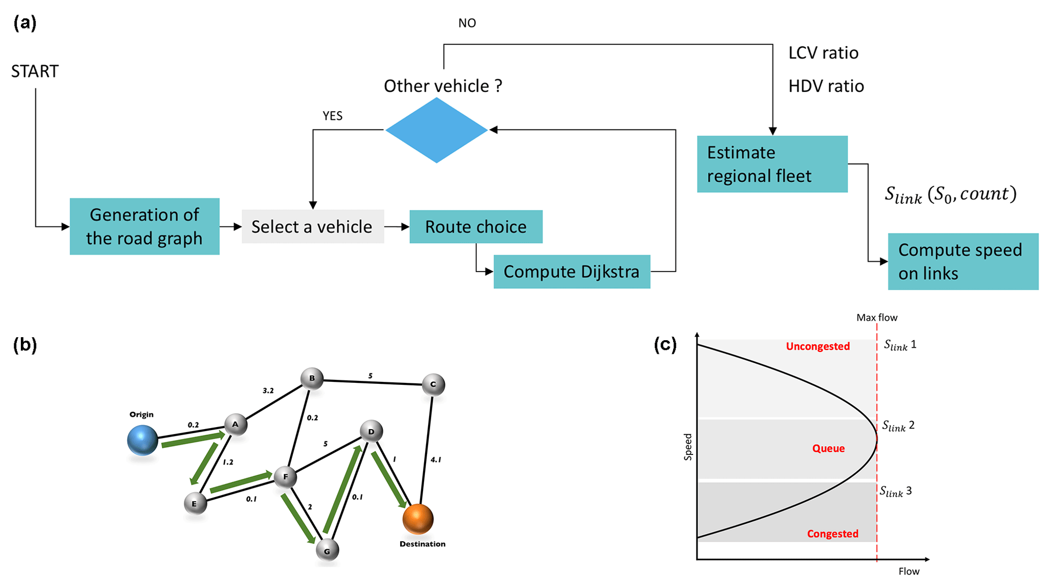
Figure 7(a) Operating diagram of the assignment of transport demand on a road network (HERMES). (b) Representation of the calculation of the shortest path based on the speeds of road sections. (c) Speed flow curve of the MOIRAI module based on three levels of road saturation.
- 3.1
Definition of the road graph. The road network is extracted from GIS road data and transformed into a graph that records the connections between different road sections, thus creating a set of edges and nodes (intersections) using the graph theory (Bondy and Murty, 1982). The speed limit is the main attribute of edges.
- 3.2
OD shortest path. HERMES computes the shortest path for each trip by solving Dijkstra's algorithm (Dijkstra, 1959). For each trip, the module identifies the nodes of the graph closest to the georeferenced O and D points. To choose the shortest path among the algorithm outputs, HERMES uses the time spent on a link as weighting.
- 3.3
Goods and interregional transport modeling. In a third step, the integration of the regional traffic flow – including the goods and the different patterns of interregional transportation – is achieved. This additional step is necessary because the MOIRAI travel request only takes into account the personal trips of agents living in the city. Interregional transport, heavy-duty vehicles (HDVs) and light commercial vehicles (LCVs) are therefore not taken into account. This is why we developed an approach that extrapolates the transportation of goods and interregional transportation trips based on a reference ratio of passenger cars to total fleet and using ratios between HDV and LCV in urban areas. Indeed, fleet composition surveys are available for many cities. They are often based on transport organizations like TFL in London.
- 3.4
Speed on link computation. Finally, HERMES integrates network congestion in its assessment of mobility. Road congestion alters speed on the road network as shown in Fig. 7c. The approach is based on the UK Department of Transport (1997) and can be represented as follows:
where the speed on the road link Slink depends on the flow Fi and length d. S0 is the free-flow speed, Sc is the congested speed, and Fc is the road link flow capacity.
This is one of the approaches suggested by Ortuzar and Willumsen (2011) to attempt to represent empirical congestion. One of the limitations of this methodology is the consideration of the impact of signaling. Other congestion functions such as that presented by Akçelik (1991) make it possible to better manage delays at junctions. On the other hand, this method requires knowledge of the location of the traffic lights. For street-level studies, the Akçelik (1991) method adds a certain realism to traffic modeling. However, it has been shown that the approach we have chosen produces a satisfactory estimate of traffic flows and road network saturation on the main roads.
Figure 8 shows the organizational chart of HESTIA, the OLYMPUS module responsible for simulating the energy demand of a building. HESTIA uses the type of dwelling, the living space of the household and its average annual energy consumption as input parameters. The main task of this module is to spatialize the energy demand in the territory.
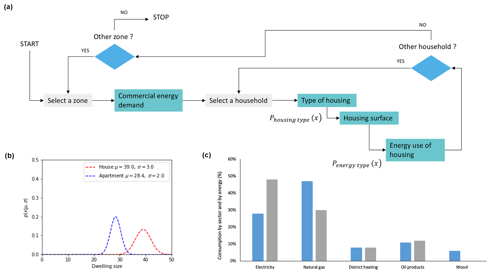
Figure 8(a) Energy demand in the regional level generator (HESTIA) flow diagram, (b) example of dwelling size distribution and (c) probability mass function of the type of energy consumed for different types of dwellings.
Swan and Ugursal (2009) proposed a review of models and methodologies for simulating the energy demand of buildings. In this framework, both top-down and bottom-up approaches are based on econometric, statistical and technical aspects of energy demand. They are mainly developed to better understand the efficiency and cost of energy policies. Because of its global approach, the top-down method lacks flexibility to create scenarios involving a change in methodology. On the other hand, some of the input parameters taken into account in a bottom-up approach go beyond what is feasible at the regional level. They require detailed data by type of building (structural properties, equipment, use) as well as individual parameters such as the orientation of buildings in relation to the sun. In OLYMPUS, the combustion emissions modeling is carried out in two stages by the HESTIA module. It lists combustion activities for residential, institutional and commercial heating, as well as domestic hot water and cooking. The process is similar to top-down approaches, but the implementation of bottom-up factors related to energy efficiency or household characteristics makes it possible to consider the implementation of energy scenarios.
The generation of energy demand in the residential sector is achieved by modeling the energy demand of each household. It depends on the size of the household, the size of the dwelling, the type of housing, the age of the dwelling and a coefficient of thermal efficiency. To generate the energy demand of the residential sector, HESTIA uses population density. The first step is to determine the ratio of collective housing to individual housing according to the population density and type of area using GAIA outputs. This ratio is clearly dependent on the country and local data such as building heights or urban density. The calculation must therefore be specific to the area of interest. In HESTIA, the distribution of household dwellings (house or apartment) is formulated as follows:
We assume that the CENTER and URBAN areas comprise a majority of buildings, while the SUBURBAN areas are where most of the individual houses are built. First of all, HESTIA starts by calculating the size of the dwelling (DWzone) according to a reference size value for different type of dwellings (SurfHT), which depends on each specific zone (γUDI) and takes into account the number of agents (n) living in the dwelling:
The energy used to heat and boil water is defined by the distribution of the energy mix, an exogenous parameter in the model:
Then, HESTIA calculates the energy consumption per household, ENcons, taking into account the size of the dwelling, DWzone, the unit energy consumption per household (ECU) and the household size (hhsz):
Finally, the module applies a climatic correction to energy consumption in order to estimate the underconsumption or overconsumption of energy due to the cold or hot climate. The degree-day (DD) is the parameter allowing us to quantify this correction as a function of the daily temperature of the considered year compared to a reference year (Jones and Harp, 1982).
The calculation of energy demand of the tertiary, institutional and commercial sectors is similar to that presented above, although it is based on annual energy consumption per employee (ECUw). In addition, the spatialization of emissions is derived from the location of employment centers and from their respective capacities (employment data by zone). Thus, the energy demand of employees can be defined as
A climate correction is also added to the consumption of this sector.
The role of the VULCAN module is to calculate pollutant emissions from both road transport and the energy consumption of buildings, which is the final step of OLYMPUS. There, the quantification of pollutant emissions is based on methodologies recommended by the European Environment Agency (EEA) guidebook for air pollutants and greenhouse gas (GHG) emissions (European Environment Agency, 2013). They rely on the use of emissions factors, which may depend on the type of fuel, but also on the age and combustion technology of the engines and stoves. The organizational chart of VULCAN is shown in Fig. 9a.
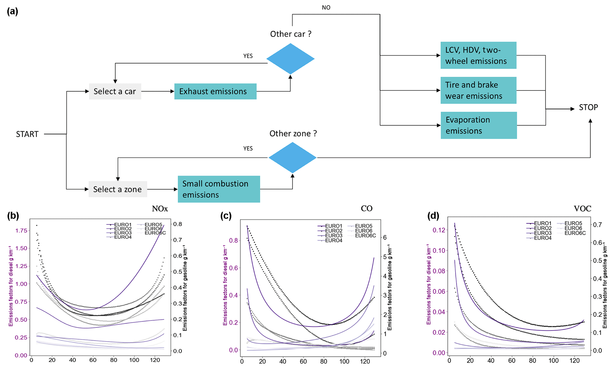
Figure 9(a) Greenhouse gas and air pollutant emissions module (VULCAN) flow diagram; (b), (c) and (d) represent NOx, CO and NMVOC emissions factors from diesel and gasoline passenger cars.
6.1 Road emissions
Road transport emissions – referred to as mobile emissions in the inventory – are calculated on linear road sections where traffic properties at a given time are homogeneous (driving cycle, average speed). For passenger vehicles, the traffic flows are derived from the travel matrices of the assignment module. From a quantitative point of view, emission factors based on traffic characteristics are applied to each section of road in order to obtain the quantities of pollutants emitted into the atmosphere per unit of time. In the literature, three main databases provide exhaust emission factors. These are HBEFA (Keller et al., 2017), COPERT (Ntziachristos et al., 2009) and MOBILE6 (US EPA, 2003). They differ in that some depend on instantaneous speeds, while others consider average driving speeds or apply to specific driving cycles such as standard highway traffic. The methodology we developed for the VULCAN emissions module is based on the recommendations of the EEA, which use COPERT emission factors based on the average speed of a vehicle during a standard driving cycle (see Fig. 9b, c, d). To be comprehensive in the counting of traffic-related emissions, we added the mechanical emission of particles from different forms of friction and abrasion during driving, as well as the evaporation of NMVOC from vehicle tanks.
A critical step in the road transport emissions modeling process is to determine the composition of the fleet, which can be inferred from the national composition data as exogenous data. In the assignment module, the choice of specific emission factors depends on the properties of the fleet (age, cylinder, fuel type), and the properties of the agent's car are defined using a conditional probability law. A second important step is the addition of cold-start emissions. This makes it possible to take into account the over-emission effect resulting from the poor performance of a vehicle starting and then running with a low-temperature engine. In order to obtain total exhaust emissions, VULCAN first calculates hot emissions factors for the stable engine regimes:
where N is the number of cars on a road link, M is the length of the road link and εhot is the emission factor. Then, VULCAN calculates cold-start emissions using an over-emission factor applied to a fraction of the distance traveled by each vehicle. This factor can be defined as
where β is the average fraction of the total distance traveled with a cold engine, and is the cold-to-hot ratio. The calculation algorithm of the cold–hot emission quotient strongly depends on European technology, on the ambient temperature and on the pollutant being considered (European Environment Agency, 2013).
The EEA offers several levels of refinement of calculations, called Tiers, the use of which depends on the information available at the input of the calculation. Tier 1 methods are based on a simple linear relationship between activity data and emission factors representing typical or averaged process conditions, which tend to be technology independent. More advanced Tier 2 methods are available for key categories, allowing us in particular to apply country-specific emission factors that depend on processing conditions, fuel qualities or abatement technologies (European Environment Agency, 2013). OLYMPUS uses the highest level of accessible detail each time. All emissions are then computed as follows:
where M is the number of traveled kilometers. For example, the calculation of emissions from LCVs, HDVs and two-wheeled vehicles is based on the EEA Tier 2 method. This methodology is used because of the excessive uncertainty of the freight fleet. HERMES generates the number N of vehicles using standard fleet composition ratios. Emissions are calculated for CORINAIR pollutants (NOx, NMVOCs, PM) and for CO2.
As mentioned above, emissions related to tire and brake wear add to exhaust emissions according to the following two equations (European Environment Agency, 2013):
where εTSP is the mass emission factor of total suspended particulate matter (TSP) for vehicles in category j (g km−1), fs is the mass fraction of TSP attributable to the particle size of class i and Ss(V) is the correction factor for an average vehicle traveling at speed V.
Finally, the VULCAN module considers the evaporation of gasoline using the following equation (European Environment Agency, 2013):
where εevap is the evaporative emission factor depending on the ambient temperature.
6.2 Building emissions
Emissions from buildings are based on the EEA guidebook for small combustion emissions (European Environment Agency, 2013). This part of the VULCAN module takes into account emissions from residential heating (fireplace, stoves, cookers, small boilers), as well as institutional and commercial heating. Small combustion emissions from the agricultural sector are not considered.
The calculation of residential and commercial–institutional emissions is based on the EEA methodology and emissions factors derived from Pfeiffer et al. (2000) and Kubica et al. (2007):
There are several types of heating and boiling equipment to consider in combustion modeling for the residential, commercial and institutional sectors (fireplaces, stoves, cookers, small boilers, space heaters, combined heat and power on a small scale). It is important to note that the composition and the age of the fleet are two crucial parameters affecting the emissions of a building, as emission factors vary with equipment and age. It has been found that improved combustion technology has a significant impact on pollutant emissions over the years. However, due to a lack of information in the literature, these parameters remain difficult to estimate accurately. For these reasons, when applying OLYMPUS to a territory, the hypotheses that we will be able to propose for the partition and the spatial distribution of the technologies of heating systems will be a determining point for the realism of the simulation.
We applied the OLYMPUS model to the Paris region. One of the reasons for this choice is that the Île-de-France region is based on a classic monocentric urban structure, with a high housing density in the center and an expanding peripheral urban area, clearly raising the problem of mobility, congestion and modal share. More generally, it is a place of intense emissions of anthropogenic pollutants that generate high annual levels of pollution. In winter, in particular, it is affected by serious problems of exposure to fine particles resulting from the combustion of biomass for domestic heating. Finally, like all areas, the region is facing the challenges of climate change and a low-carbon economy, a challenge for which road traffic control could prove to be a particularly effective lever. In this area, the quality of the available input data would allow for greater robustness and better reliability of the simulations.
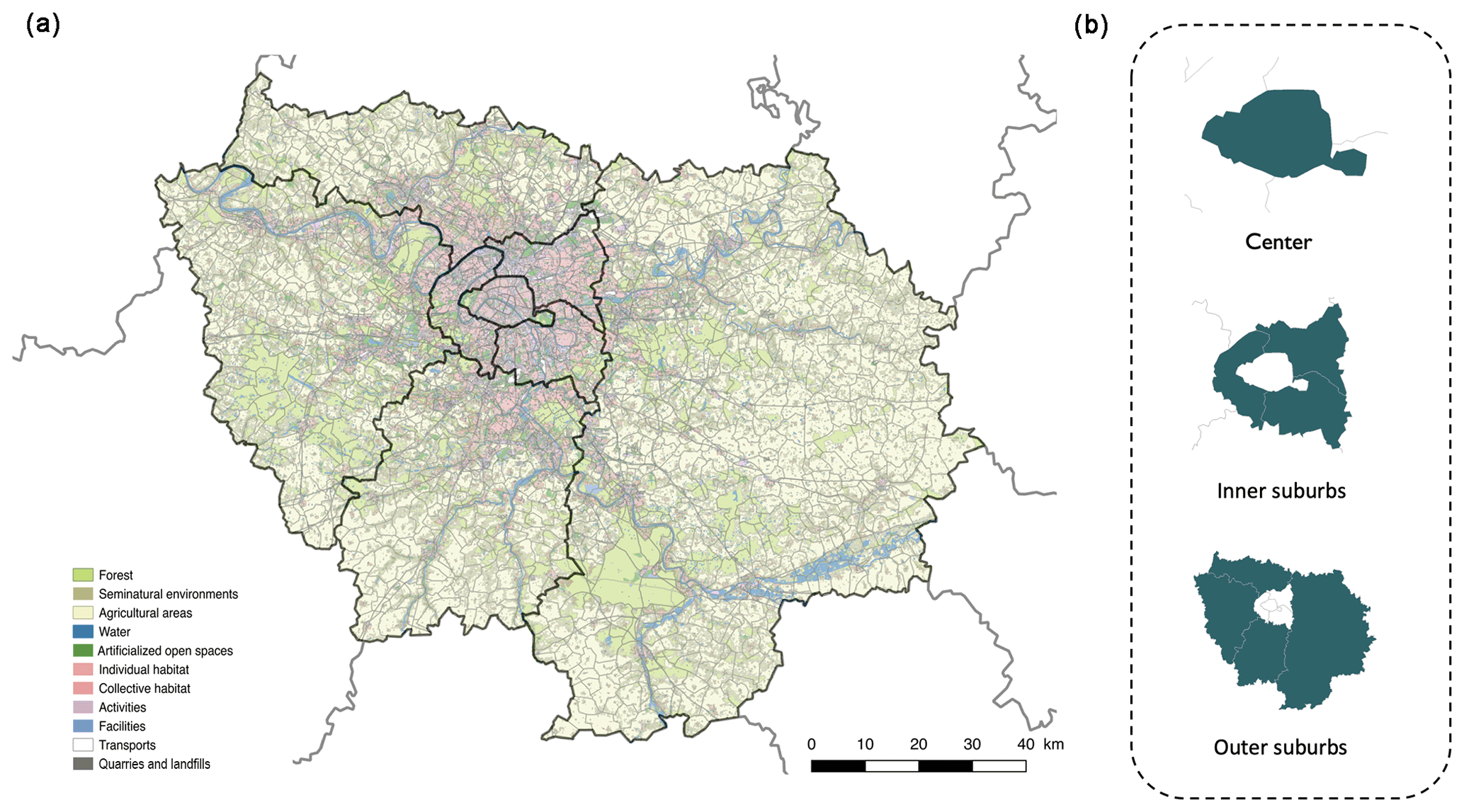
Figure 10(a) Representation of the Île-de-France region (greater Paris) and the land use. (b) Representation of the Île-de-France subdivision.
We conducted a 1-year simulation with OLYMPUS in the Paris region. The input data selection, working assumptions and configurations selected for the OLYMPUS model are described below. The results of the emissions calculations are then analyzed. The source code can be obtained from the LISA website at http://www.lisa.u-pec.fr/~aelessa/OLP (Elessa Etuman, 2018) or upon request to the authors.
7.1 Configuration
The simulations were carried out for the year 2009, for which we had a large database of input data (surveys, censuses, inventories). The simulation domain is the Île-de-France region (greater Paris). It is a monocentric urban area with a population density of 21 000 inhabitants km−2 in the city center and a density that decreases radially to the remote suburbs, which are predominantly rural (Fig. 10).
The population in this territory is greater than 11 million inhabitants. In terms of transport infrastructure, Paris is considered by the Institute for Transportation and Development Policy as the city with the most efficient network (Marks, 2016). Individual mobility is 3.87 trips per person per day on average, with 41 million trips made each day in the region. The majority of trips (70 %) do not include travel to the center of the metropolis: trips in Île-de-France are mostly short (4.4 km on average) and close to home.
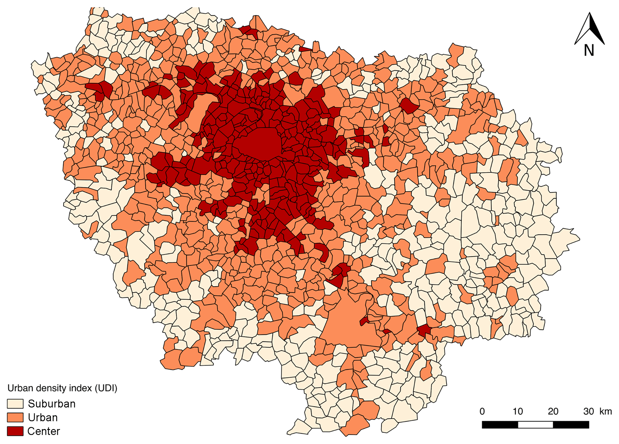
In OLYMPUS, the computing space unit is TAZ. Here, it comes from the National Institute of Statistics (INSEE), which has set up a specific division of the territory called IRIS that gathers between 1800 and 5000 inhabitants. For our domain, this choice leads to the constitution of 1300 TAZs. Figure 11 illustrates the division of the region into IRIS, as used by OLYMPUS.
The modeling of anthropogenic combustion emissions resulting from individual activities requires a very large amount of data. The main sources of these data are shown in Table 1. To generate the synthetic population in GAIA, we used aggregated data from the census of the city, mainly derived from INSEE. They include the distribution of the population in the territory by age and gender, the number of households by IRIS, and the average distribution of households by type (single, couples, family, single-parent family). Mobility calculations in MOIRAI are based on several types of data, mainly surveys or national statistical databases. First, the accessibility of the area by public transport was assessed on the basis of the density of the public transport networks provided by the STIF regional transport agency. Regarding the attractiveness of urban subareas, the creation of attractive WORK zones is based on INSEE census data, which provide the number of jobs per municipality. The average distance at which agents can be attracted to an occupational zone is then deduced from the city's overall transport survey (STIF, 2012). The total mobility of the agents is also conditioned by the total number of trips per day weighted according to the number of priorities of the agents. Here, the average number of daily trips was estimated from local surveys, and we assumed that trips other than those related to commuting were characterized by the same average distance, which is not the case in reality. For the OTHERS category, agent interest in a given activity results from two main parameters: the number of households in the immediate vicinity of an activity and the estimated average distance traveled to reach this activity. Once these values are set, the determining parameter for carrying out the activity will be the estimated duration of the trip. Here, this parameter was derived from THEMIS, whose calibration had been achieved through an online application based on GTFS data from all regional transport agencies. It allows for the constitution of a matrix of average transport times between the different classes of urbanized areas (UTAI). In the end, the combination of transport network data and population density makes it possible to calculate the accessibility of any area of activity.
Table 1OLYMPUS parameterization for the greater Paris simulation.
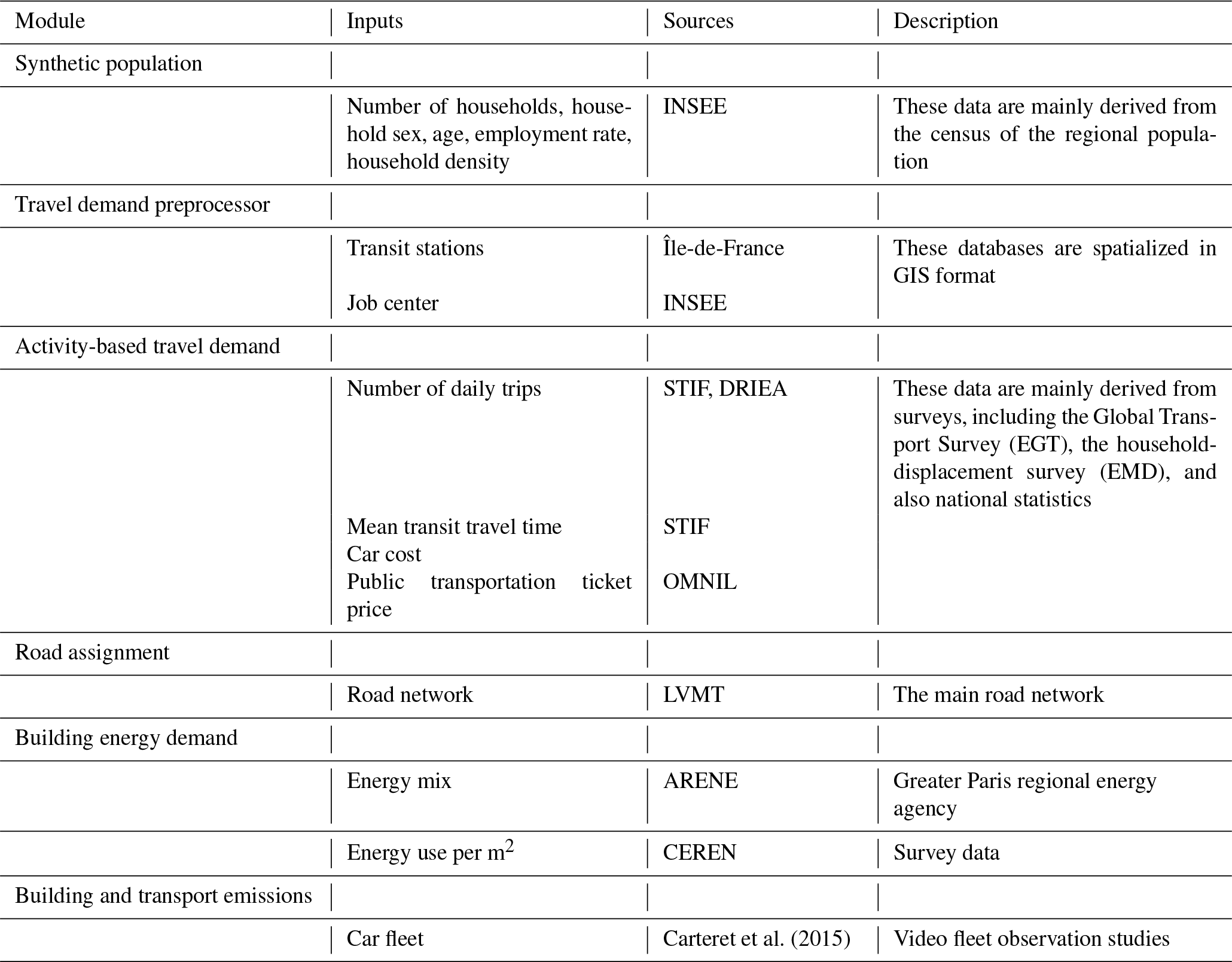
The fleet of vehicles used in HERMES dates back to 2009 and is based on the Carteret et al. (2015) survey. It includes passenger cars, LCVs and HDVs. This study is based on the use of video observation to characterize a fleet of vehicles, then comparing to the global transport survey. The regional fleet of stoves and fireplaces was not estimated, so it was not included. We simply assumed here that individual heating modes, including wood heating, came mainly from individual dwellings. The total energy demand in the territory was estimated from data from ARENE surveys (Regional Agency for the Environment and New Energies) providing unitary consumption of households in Île-de-France, but also from information on the average household housing area, by type of household and by place of residence, provided by CEREN (Center for Economic Research on Energy). The consumption modeling of the commercial–institutional sector was carried out on the basis of annual consumption per employee in the commercial–institutional sector (CEREN, 2015).
7.2 Results and discussion
Figure 11 shows the results of synthetic population modeling obtained by performing probability functions from aggregated census data. It also shows that we obtain a realistic representation of the variations in household density in the territory. Regarding the characteristics of the population (Fig. 11), note that OLYMPUS accurately captures the age distribution of the inhabitants of greater Paris compared to data from the INSEE census. However, it should be noted that OLYMPUS underestimates the elderly population by a factor of about 2 – or more for the oldest age group – and underestimates the child population by 24 %. These are age groups associated with low mobility, and for the oldest age group this represents only a small proportion of the total number of agents. Thus, based on the low distribution error (in %) of the labor force, we consider the model to generate an acceptable synthetic population for transport modeling. Finally, the average attributes of the agents used as forcing in an aggregated form are correctly represented in the synthetic population: gender data, unemployment rate, distribution of household types and average household size. Because OLYMPUS relies on Bayesian statistics to generate a synthetic population, to obtain representative results it is necessary to initially have a large database containing specific information on the distribution of agent characteristics in the population. Thus, thanks to the transcription of stochastic variables, the synthetic population has great similarities with the population studied. Nevertheless, this approach produces limited variability in socioeconomic parameters within the distribution, offering a simulated population too close to the average characteristics of the actual population. In this simulation, we limited ourselves to the use of a three-level UDI and the division of the domain into 1300 TAZ. In order to define the most sensitive components of the urban system modeled with OLYMPUS, it will be interesting to test the sensitivity of the outputs of the model to the increase in the spatial variability of the properties of the agents, to the use of a wider range of indices and to a greater number of TAZs.
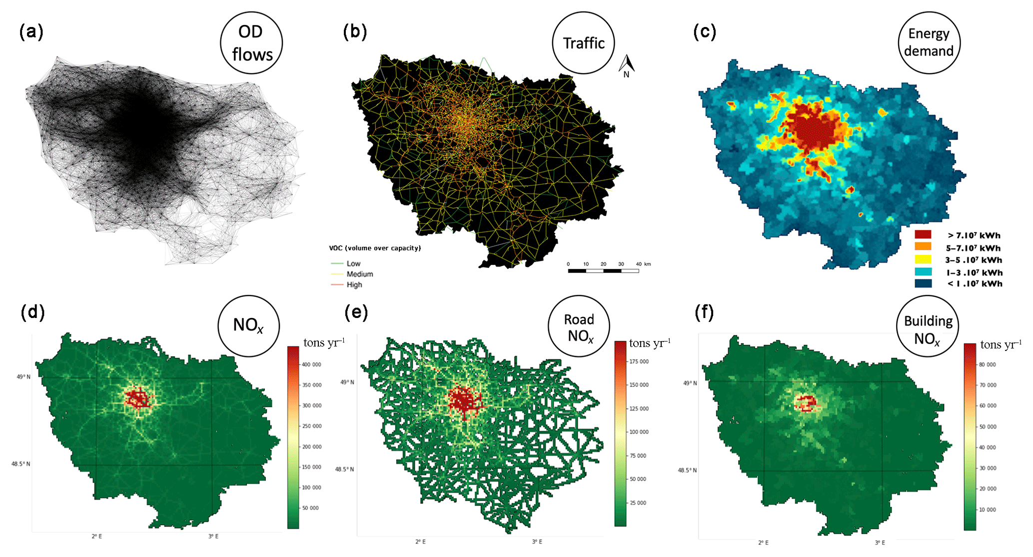
Figure 12(a) Representation of all origin–destination flows generated by MOIRAI motion request module. (b) Representation of daily road traffic in greater Paris in terms of volume over capacity (VOC), (d) nitrogen oxide emissions in Île-de-France from road transport and residential–commercial–institutional sector (OLYMPUS), (e) focus on emissions from road transport, (f) focus on emissions from the residential–commercial–institutional sector.
Agent mobility modeling was carried out using the OD matrices of home–work trips generated by MORAI based on data from the employment survey in greater Paris. Figure 12a and b illustrate the mobility of the synthetic population modeled by OLYMPUS. Figure 12a shows the complete set of routes built by OLYMPUS, while Fig. 12b shows the saturation of the road network more specifically in terms of volume on capacity (VOC). This last map shows very high values of the VOC factor in the city center and in the suburbs close to the center, confirming the monocentric nature of the megalopolis perceived by OLYMPUS. The same centrality of the simulated mobility is found in Fig. 12a, which presents trajectories strongly oriented towards the heart of the megacity. This result was compared to mobility indicators from transport surveys. Table 2 shows the comparison of simulated and survey-based data on average number and length of trips per day. The simulated data are very realistic, with a difference of only 4 % for the total number of trips per day and per agent in Île-de-France and an overestimate of 6.9 % for the average trip length compared to average values of the transport survey. The total number of trips and the modal shares are very close to reality (less than 3 % difference with field data). If we consider differences of less than 5 % between simulated and observed values to be satisfactory and differences of less than 3 % to be very satisfactory, then this first comparison work reveals that OLYMPUS simulates the main characteristics of regional transport demand satisfactorily to very satisfactorily. Only the simulated average trip length is not completely satisfactory (+6.9 %). In order to evaluate the OLYMPUS results in more detail (and to propose a comprehensive correction of the average trip length), future works could include a map of the simulated and observed mobility. This spatialized analysis would take into account the fraction, length and the modal share of the trips made between the different zones (center to center, center to near suburbs, suburb to suburb). Such an evaluation requires a lot of data to be processed, but it could allow for both a more refined evaluation of OLYMPUS outputs and a diagnosis of mobility levers in the model.
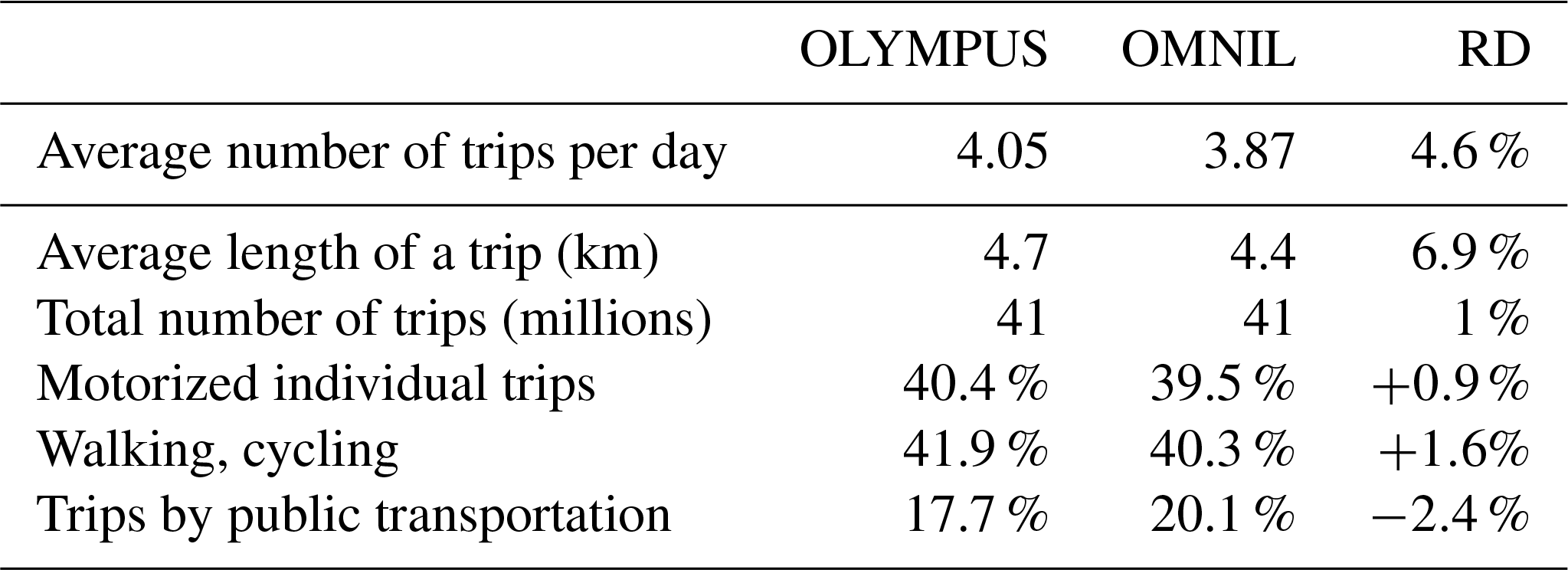
Figure 12c shows a map of simulated energy demand in greater Paris. The results show a fairly logical positive dependence on the total population, with maximum demand at the center of the agglomeration. The total energy consumption of greater Paris (including energy demand for electricity) was 303 TWh in 2009 according to ARENE (2013). The energy consumption from the residential, commercial and institutional sectors represents more than 50 % of this total. The modeling of the regional energy demand (HESTIA) is consistent with surveys, the difference being around +9.6 %.
Emission modeling from both road transport and building heating was carried out by calculating the linear and surface emissions of air pollutants and greenhouse gases for each road segment and consumption unit. It was followed by a projection of the emissions on a regular grid of kilometric resolution. The results, illustrated in Fig. 12d for nitrogen oxides (NOx), a family of gaseous species emitted during combustion processes, show very good consistency with the spatial emitting patterns in Île-de-France (major roads, types and density of housing by zone). The total emissions of OLYMPUS are then compared to two reference emission inventories: the AIRPARIF air quality network inventory and that of the European network EMEP. To this end, we have extracted for each inventory the activity sectors corresponding to the emissions calculated by OLYMPUS. The comparison is presented as histograms in Fig. 13 for NOx and for two size sections of particulate matter: PM2.5 and PM10. It should be noted that the calculation methods differ between the two “reference” inventories: AIRPARIF develops bottom-up approaches from local data collection, while EMEP inventories are derived from national totals by species, which are spatially disaggregated using top-down approaches. In addition, the comparison with the EMEP inventory cannot be done in detail due to the lack of information on the subsectors of activity in the EMEP data.
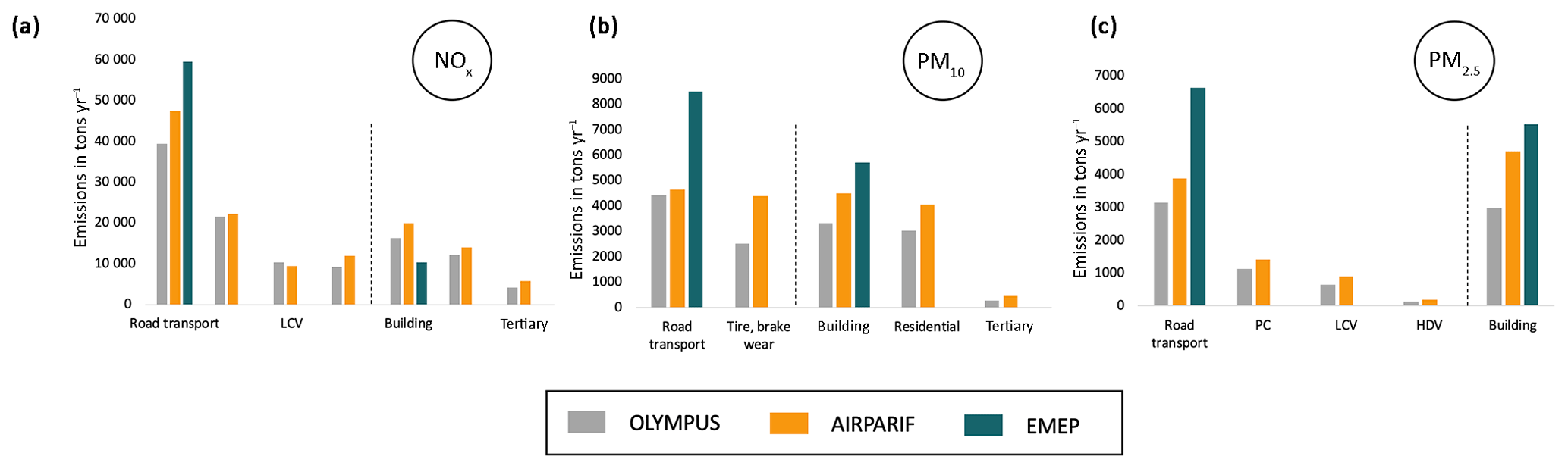
Figure 13Emissions comparison with local and regional inventories for (a) nitrogen oxides, (b) particulate matter with a diameter of 10 µm or less, and (c) fine particles with a diameter of 2.5 µm or less.
The emissions produced by OLYMPUS, although slightly underestimated compared with the emissions of AIRPARIF, are considered here as very satisfactory. Indeed, the OLYMPUS emissions, either total or by vehicle type, show differences of less than 20 % with the AIRPARIF values for nitrogen oxides (NOx) and particulate matter (PM2.5 and PM10). The variations in the AIRPARIF emissions from one subgroup to another (PC, LCVs, HDVs) is also reproduced well by OLYMPUS. This is remarkable considering that OLYMPUS (which constructs mobility matrices using a gravity approach and relying on the choice of individuals) has very few forcing data in common with AIRPARIF (which mainly uses road count data, vehicle sales and registration, fuel consumption surveys). In particular, although both inventories use the COPERT methodology, other sources of differences exist, notably in the hypotheses about the fleet in circulation. An earlier study by Timmermans et al. (2013) confirms that the observed discrepancies in emissions are consistent with the fact that different approaches are used. Indeed, the authors indicate that the expected gap between emission inventories based on different modeling assumptions (choices on the cold-start fraction, fuel evaporation emissions modeling, engine fleet) is expected to be 20 % at the minimum. By contrast, particulate matter emissions related to abrasion seem to be more severely underestimated by OLYMPUS compared with the AIRPARIF database (−30 %), but there are currently very few ways to estimate real emission values. Deviations from the EMEP inventory are greater, which can be explained by the fact that the EMEP approach is coarse and strongly overestimates some emissions compared with the AIRPARIF inventory. Nevertheless, the tendency to underestimate emissions in OLYMPUS may reflect the lack of consideration of specific sources in the model. In particular, the model calculates the transport of goods on the basis of occupancy rates on urban roads and does not take into account interregional mobility, the city being considered here as a closed system. This largely explains the underestimation of traffic at the borders of the region and in certain rural areas (not shown here). Taking this source into account is considered as a priority evolution of the model.
In addition, the issue of congestion should not be treated superficially in a model like OLYMPUS because it affects the decision of the agents along their commute and contributes to an increase in emissions. At present, congestion is managed by the representation of speed classes on the main axes, but more dynamic management of this process is envisaged. One of the methods identified to address this problem is the establishment of an iterative process between congestion and the choice of agents and the refinement of the representation of speed as a function of the occupancy rate of the lanes. This is also what future developments of the platform will focus on.
The activity sector that shows the highest differences between the two regional inventories is residential combustion, with OLYMPUS underestimating the value of the AIRPARIF inventory for PM10 by a factor of 2. However, we mentioned that we do not have information about local combustion equipment data and that equipment technology is a determinant factor of emissions related to heating. In particular, wood burning is responsible for more than 90 % of particulate matter emissions in this sector. In addition, AIRPARIF has its own modeling assumptions for residential heating, including industrial heaters not based on local data, as well as an estimate of the number of chimneys and stoves. Furthermore, there is no specific survey on combustion technologies in the commercial and institutional sectors. This point explains the very large variability of emission estimates in the different inventories. The comparison between inventories can hardly overcome this lack of constraints. We should therefore consider the range of values given by OLYMPUS to be consistent with the estimates of the reference inventories, and our work contributes to the improvement of the evaluation of household combustion emissions in Île-de-France.
Finally, as for the total number of trips, the structure of trips and the modal share, the results simulated by OLYMPUS are quite close to the data used as a reference (surveys or models), which validates each of the steps in OLYMPUS: the representation of the average number of trips per agent, the division of urban areas into attractiveness classes and the use of the utility function for modal choices. As a consequence, our modeling approach appears relevant for analyzing the links between city, population, mobility, energy consumption and pollutant emissions. A better consideration of the effects of freight transport and congestion will make analyses conducted with OLYMPUS even more robust.
Nevertheless, to go further in the analysis of the results of OLYMPUS, we must examine the question of rationality. Mobility modeling is based primarily on the theory of random utility, in which each agent in the synthetic population is considered to make rational choices for transportation mode. Utility is a notion used in economics, and it obviously has several limitations as described by the economists Becker and Murphy (1988). First, it requires that agents have full access to information in order to make the most rational decision, which is unrealistic. It is more likely that different agents will have access to partial and different sets of information when making decisions. Second, the time given to the agent to make a decision influences the final choice, which is not taken into account in this approach. Finally, the maximum utility of an action may not be the same for each person since it depends on the preferences and weights given to each of the various elements that compose the utility function. Despite this, Wegener (2004) presented an exhaustive list of the main land use transport interaction models, including those using the random utility such as EMME, VISSUM and MATSIM. This gives the “utility” approach more robustness because of the reliable predictions made by these models for typical behaviors of people within a group. To better test the implications of rational choice in OLYMPUS, it would be interesting to test the response of the mobility of the agent to the weighting of the utility function or even to an increase in the variability of its expression.
In the current environmental context, in which the problems of air quality and climate change are exacerbated in cities, it is absolutely necessary to develop integrated urban modeling capable of providing a diagnosis of the effects of urban public policies on energy consumption, pollutant emissions, air quality and exposure of the population. The OLYMPUS model has been developed to meet this need. Indeed, OLYMPUS is an emission model calculating pollutant emissions from anthropogenic combustion in the city (road traffic, building heating, cooking, etc.) and designed to integrate into an urban modeling platform consisting of a set of disciplinary models. In this platform, OLYMPUS needs to be forced by data on morphology and urban services (land use, population density, transport supply, etc.) that can be derived from surveys or obtained from a model providing urban growth from public policy scenarios (densification or urban sprawl, improvement of public transport, green belts).
Then, OLYMPUS builds a synthetic population corresponding to the urban scenario. In a second step, using an individual decision-based approach, it provides mobility matrices and spatialized energy demand to account for agent activities in the city. The energy demand is finally used to produce a pollutant and GHG emission inventory at a kilometric scale for the whole urban area. The data produced by OLYMPUS allow for much more advanced scenarios than the usual air quality models (they only consider a regulatory percentage of emission reductions). OLYMPUS simulates the scenario elements needed to provide decision support that takes into account the collective appropriation of environmental policies as well as the impact of urban forms on transport demand and mobility, which is absolutely not the case in the current literature.
OLYMPUS has been implemented in the Paris region. The emissions inventory produced with this model shows a fairly good understanding of the individual and collective activities that consume energy in this area. Although OLYMPUS outputs (pollutant emissions) have been shown to be quite comparable with the AIRPARIF emissions inventory, assumptions about congestion, lack of representation of freight transport and interregional mobility may be responsible for an overall underestimation of emissions. The representation of these processes will be improved in the very short term in OLYMPUS. In the longer term, other evolutions have to be considered for OLYMPUS.
Uncertainties in domestic–residential–commercial heating emissions can be reduced by changing the energy demand setting in OLYMPUS and integrating local parameters such as building height or sunlight. However, a significant improvement could be immediately achieved by using a realistic speciation of energy consumption according to the type of agent in the population. Although these data are not fully available for the Paris region, these improvements should be considered for future works.
Improvements can be included in the representation of agent choices. It would therefore be interesting to introduce additional socioeconomic segregation parameters (for example, household income) and their impact on mobility choices. This could allow us to highlight social discrimination in our emissions analysis. It may also be interesting to set up feedback loops between OLYMPUS modules to simulate agent interactions and develop a multi-agent model. For example, the discrete choice module can be coupled to the path assignment module to make a feedback between congestion and modal choice. Finally, among the developments envisaged for the model, it would also be interesting to test the implementation of time-dependent attractiveness classes, which may modify the spatial distribution of mobility outside working hours. In addition, the sequencing of activities that influence the temporal variability of the activities is a parameter that can be improved by adding a specific program according to the characteristics of the agents in the synthetic population.
In addition to OLYMPUS developments, one of our main prospective goals is to implement OLYMPUS in other cities with different morphologies in order to test the transposability of the model and to have a broader vision of city responses to political forcing.
OLYMPUS is published as an integrated model of pollutant and greenhouse gas emissions. The source code can be obtained from the LISA website at http://www.lisa.u-pec.fr/~aelessa/OLP (Elessa Etuman, 2018) or upon request to the authors. The version presented here corresponds to OLYMPUS v1.0. Some improvements will be made and OLYMPUS 1.0 will be updated for the latest version of the code. It is possible to run the model with a sample of data available in the input data directory.
| ABTD | Activity-based travel demand |
| GAIA | Synthetic population generator module |
| GIS | Geographic information system |
| HBS | Home-based sequence |
| HDV | Heavy-duty vehicle |
| HERMES | Trip assignment module |
| HESTIA | Building energy demand module |
| LCV | Light commercial vehicle |
| MHBS | Multiple home-based sequence |
| MOIRAI | Population agent mobility generator module |
| NHBS | Nonhome-based sequence |
| OD | Origin–destination |
| OLYMPUS | Integrated emissions model |
| PC | Passenger car |
| PMF | Probability mass functions |
| TAZ | Travel analysis zone |
| THEMIS | Activity-based travel demand preprocessing module |
| UDI | Urban density index |
| UTAI | Urban transport accessibility index |
| VULCAN | Emissions module |
AEE designed and implemented the entire model. IC coordinated the study.
The authors declare that they have no conflict of interest.
This work was performed using HPC resources from GENCI-CCRT (grant 2017-t2015017232). This work also received support from the French National
Agency for Research (ANR-14-CE22-0013) and the Île-de-France region (DIM
R2DS). We also acknowledge AIRPARIF and the LABEX Urban Futures.
Edited by: Christoph Knote
Reviewed by: two anonymous referees
Akçelik, R.: Travel time functions for transport planning purposes: Davidson's function, its time dependent form and alternative travel time function, Aust. Road Res., 21, 49–59, 1991.
Amann, M., Klimont, Z., and Wagner, F.: Regional and Global Emissions of Air Pollutants: Recent Trends and Future Scenarios, Annu. Rev. Env. Resour., 38, 31–55, https://doi.org/10.1146/annurev-environ-052912-173303, 2013.
Antoni, J., Tannier, C., Vuidel, G., and Hirtzel, J.: MobiSim?: un modèle multi-agents et multi-scalaire pour simuler les mobilités urbaines, in Modéliser la ville, Forme urbaine et politiques de transport, edited by: Antoni, J.-P., Paris, France, 50–77, 2010.
ARENE: La facture énergétique francilienne, Paris, France, available at: https://www.areneidf.org/sites/default/files/facture_ energetique_francilienne_v9_1.pdf (last access: 24 October 2018), 2013.
Bandeira, J. M., Coelho, M. C., Sà, M. E., Tavares, R., and Borrego, C.: Impact of land use on urban mobility patterns, emissions and air quality in a Portuguese medium-sized city, Sci. Total Environ., 409, 1154–1163, https://doi.org/10.1016/j.scitotenv.2010.12.008, 2011.
Banos, A., Boffet-Mas, A., Chardonnel, S., Lang, C., Marilleau, N., and Thévenin, T.: Simuler la mobilité urbaine quotidienne?: le projet MIRO, in Mobilités urbaines et risques des transports, edited by: Banos, A. and Thévenin, T., Hermès, 2010.
Barcelo, J., Ferrer J. L., and Montero, L.: AIMSUN: Advanced Interactive Microscopic Simulator for Urban Networks, Vol. I, System Description, and Vol. II, Users Manual, Departamento de Estadistica e Investigacion Operativa, Facultad de Informatica, Universidad Politecnica de Cataluna, 1989.
Becker, G. S. and Murphy, K. M.: A Theory of Rational Addiction, J. Polit. Econ., 96, 675–700, 1988.
Beckman, R. J., Baggerly, K. A., and McKay, M. D.: Creating synthetic baseline populations, Transp. Res. Part A Policy Pract., 30, 415–429, https://doi.org/10.1016/0965-8564(96)00004-3, 1996.
Bondy, J. A. and Murty, U. S. R.: Graph Theory with Applications, Oper. Res. Quart., 28, 1–270, https://doi.org/10.2307/3008805, 1982.
Borrego, C., Martins, H., Tchepel, O., Salmim, L., Monteiro, A., and Miranda, A. I.: How urban structure can affect city sustainability from an air quality perspective, Environ. Model. Softw., 21, 461–467, https://doi.org/10.1016/j.envsoft.2004.07.009, 2006.
Bretagnolle, A., Pumain, D., Vacchiani-Marcuzzo, C., Bretagnolle, A., Pumain, D., and The, C. V.: The organisation of urban systems, available at: https://halshs.archives-ouvertes.fr/halshs-00459713/document (last access: 24 October 2018), 2010.
Broquereau L.: DAVISUM, un outil de modélisation multimodale des transports, Rev. Générale des Routes, no. 773, 37–41, 1999.
Caliper Corporation: Travel Demand Modeling with TransCAD, available at: https://www.caliper.com/tcovu.htm (last access: 24 October 2018), 2010.
Cameron, G., Wylie, B. J. N., and McArthur, D.: Paramics: moving vehicles on the connection machine, Proc. 1994 ACM/IEEE Conf. Supercomput., 94, 291–300, https://doi.org/10.1109/SUPERC.1994.344292, 1994.
Carteret, M., Andre, M., and Pasquier, A.: Méthode d'estimation des parcs automobiles et de l'impact de mesures de restriction d'accès sur les émissions de polluants, available at: https://hal.archives-ouvertes.fr/hal-01232521/document (last access: 24 October 2018), 2015.
Castiglione, J., Bradley, M., and Gliebe, J.: Activity-Based Travel Demand Models: A Primer, edited by: Transportation Research Board, Washington, DC, 2015.
CEREN: Données statistiques du CEREN, available at: https://www.ceren.fr/publications/ (last access: 24 October 2018), 2015.
Delling, D., Pajor, T., and Werneck, R. F.: Round-Based Public Transit Routing, Proc. 14th Meet. Algorithm Eng. Exp., 130–140, https://doi.org/10.1287/trsc.2014.0534, 2012.
Deming, W. E. and Stephan, F. F.: An a least squares adjustment of a sampled frequency table when the expected marginal totals are known, Ann. Math. Stat., 11, 428–444, 1940.
De Ridder, K., Lefebre, F., Adriaensen, S., Arnold, U., Beckroege, W., Bronner, C., Damsgaard, O., Dostal, I., Dufek, J., Hirsch, J., IntPanis, L., Kotek, Z., Ramadier, T., Thierry, A., Vermoote, S., Wania, A., and Weber, C.: Simulating the impact of urban sprawl on air quality and population exposure in the German Ruhr area. Part II: Development and evaluation of an urban growth scenario, Atmos. Environ., 42, 7070–7077, https://doi.org/10.1016/j.atmosenv.2008.06.044, 2008.
Dibbelt, J., Pajor, T., Strasser, B., and Wagner, D.: Intriguingly Simple and Fast Transit Routing?, 288094, 1–12, available at: http://i11www.iti.uni-karlsruhe.de/extra/publications/dpsw-isftr-13.pdf (last access: 24 October 2018), 2013.
Dijkstra, E. W.: A Note on Two Probles in Connexion with Graphs, Numer. Math., 1, 269–271, https://doi.org/10.1007/BF01386390, 1959.
EEA: Exceedance of air quality limit values in urban areas, 26, available at: http://www.eea.europa.eu/data-and-maps/indicators/exceedance-of-air-quality-limit-3/assessment (last access: 24 October 2018), 2015.
EEA: Air Quality e-Reporting Database, available at: https://www.eea.europa.eu/data-and-maps/data/aqereporting (last access: 24 October 2018), 2016.
Elessa Etuman, A.: OLP, available at: http://www.lisa.u-pec.fr/~aelessa/OLP, last access: 5 December 2018.
European Commission: Survey on perception of quality of life in 75 European cities, available at: http://ec.europa.eu/regional_policy/sources/docgener/studies/pdf/urban/survey2009_en.pdf (last access: 24 October 2018), 2010.
European Environment Agency: EMEP/EEA air pollutant emission inventory guidebook – 2013, available at: https://www.eea.europa.eu/publications/emep-eea-guidebook-2013 (last access: 24 October 2018), 2013.
Gomes, G. and May, A.: A Microsimulation Model of a Congested Freeway using VISSIM, Transp. Res., 8816, 2004.
Hagberg, A. A., Schult, D. A., and Swart, P. J.: Exploring network structure, dynamics, and function using NetworkX, Proc. 7th Python Sci. Conf. (SciPy 2008), (SciPy), 11–15, 2008.
Hao, J., Hatzopoulou, M., and Miller, E.: Integrating an Activity-Based Travel Demand Model with Dynamic Traffic Assignment and Emission Models, Transp. Res. Rec. J. Transp. Res. Board, 2176, 1–13, https://doi.org/10.3141/2176-01, 2010.
Hatzopoulou, M., Miller, E. J., and Santos, B.: Integrating Vehicle Emission Modeling with Activity-Based Travel Demand Modeling: Case Study of the Greater Toronto, Canada, Area, Transp. Res. Rec., 2011, 29–39, https://doi.org/10.3141/2011-04, 2008.
Hickman, J., Hassel, D., Joumard, R., Samaras, Z., Sorenson, S., and Laboratory, T. R.: Methodology for calculating transport emissions and energy consumption, Deliv. 22 Proj. MEET, (3011746), 362, 1999.
Huff, D. L.: Defining and estimation a trading area, J. Marketing, 28, 34–38, 1964.
Hulchanski, B. Y. J. D.: Income Polarization Among Toronto ' s Neighbourhoods, 1970–2005, available at: http://homelesshub.ca/sites/default/files/Three-Cities-Within-Toronto_2010_Final.pdf (last access: 24 October 2018), 2010.
Hülsmann, F., Gerike, R., and Ketzel, M.: Modelling traffic and air pollution in an integrated approach – the case of Munich, Urban Clim., 10, 732–744, https://doi.org/10.1016/j.uclim.2014.01.001, 2014.
International Energy Agency: Energy and Air Pollution, World Energy Outlook – Spec. Rep., 266, https://doi.org/10.1021/ac00256a010, 2016.
IPCC: Revised 1996 IPCC Guidelines for National Greenhouse Gas Inventories, Annex 2: IPCC and Corinair Source Categories, 1996.
Jones, L. K. and Harp, S. L.: Residential Energy Analysis Using Modified Degree-Day Procedures, T. ASAE, 25, 1387–1390, 1982.
Keller, M., Hausberger, S., Matzer, C., Wüthrich, P., and Notter, B.: HBEFA Version 3.3., available at: http://www.hbefa.net/e/documents/HBEFA33_Documentation_20170425.pdf (last access: 5 December 2018), 2017.
Klimont, Z., Kupiainen, K., Heyes, C., Purohit, P., Cofala, J., Rafaj, P., Borken-Kleefeld, J., and Schöpp, W.: Global anthropogenic emissions of particulate matter including black carbon, Atmos. Chem. Phys., 17, 8681–8723, https://doi.org/10.5194/acp-17-8681-2017, 2017.
Kubica, K., Paradiz, B., and Dilara, P.: Small combustion installations?: Techniques, emissions and measures for emission reduction, JRC Scientific and technical Reports, Luxembourg, available at: http://publications.jrc.ec.europa.eu/repository/handle/JRC42208 (last access: 5 December 2018), 2007.
Kwan, M. P. and Weber, J.: Individual accessibility revisited: The implications of changing urban form and human spatial behavior, Geogr. Anal., 35, 341–353, 2003.
Le Néchet, F.: Aprroche multiscalaire des liens entre mobilité quotidienne, morphologie et soutenabilité des métropoles européennes, Cas de Paris et de la région Rhin-Ruhr, 496, 2010.
Mahmassani, H. S., Fei, X., Eisenman, S., Zhou, X., and Qin, X.: DYNASMART-X Evaluation for Real-Time TMC Application: Chart Test Bed, 2005.
Malayath, M. and Verma, A.: Activity based travel demand models as a tool for evaluating sustainable transportation policies, Res. Transp. Econ., 38, 45–66, https://doi.org/10.1016/j.retrec.2012.05.010, 2013.
Manins, P. C.: Regional air pollution modelling for planners, Terr. Atmos. Ocean. Sci., 6, 393–401, 1995.
Marks, M.: People Near Transit?: People Near Transit?, available at: https://www.itdp.org/wp-content/uploads/2016/10/People-Near-Transit.pdf (last access: 24 October 2018), 2016.
Marquez, L. O. and Smith, N. C.: A framework for linking urban form and air quality, Environ. Model. Softw., 14, 541–548, https://doi.org/10.1016/S1364-8152(99)00018-3, 1999.
Martins, H.: Urban compaction or dispersion? An air quality modelling study, Atmos. Environ., 54, 60–72, https://doi.org/10.1016/j.atmosenv.2012.02.075, 2012.
Mathis, P., Bailleul, H., Buguellou, J.-B., and Feildel, B.: Cohérence entre politique des transports et politique d'aménagement?: le cas de Mulhouse par modélisation prospective, Rapport PREDIT – ADEME, Tours, France, 2008.
McFadden, D.: Conditional Logit Analysis of Qualitative Choice Behaviour, in: Frontiers in Econometrics, edited by: P. Zarembka, Academic Press, New York, 1, 1974, 105–142, 1973.
Melia, S., Parkhurst, G., and Barton, H.: The paradox of intensification, Transp. Policy, 18, 46–52, https://doi.org/10.1016/j.tranpol.2010.05.007, 2011.
Menut, L., Bessagnet, B., Khvorostyanov, D., Beekmann, M., Blond, N., Colette, A., Coll, I., Curci, G., Foret, G., Hodzic, A., Mailler, S., Meleux, F., Monge, J.-L., Pison, I., Siour, G., Turquety, S., Valari, M., Vautard, R., and Vivanco, M. G.: CHIMERE 2013: a model for regional atmospheric composition modelling, Geosci. Model Dev., 6, 981–1028, https://doi.org/10.5194/gmd-6-981-2013, 2013.
Miyazaki, K., Eskes, H., Sudo, K., Boersma, K. F., Bowman, K., and Kanaya, Y.: Decadal changes in global surface NOx emissions from multi-constituent satellite data assimilation, Atmos. Chem. Phys., 17, 807-837, https://doi.org/10.5194/acp-17-807-2017, 2017.
Müller, K. and Axhausen, K. W.: Hierarchical IPF: Generating a Synthetic Population for Switzerland, Eidgenössische Technische Hochschule Zürich, Institution for Transport Planning and Systems, Zurich, Switzerland, available at: http://www.sustaincity.org/publications/SCCI_Hierarchical_IPF.pdf (last access: 5 December 2018), 2011.
Ntziachristos, L., Gkatzoflias, D., and Kouridis, C.: COPERT: A European road transport emission inventory model, April 2016, https://doi.org/10.1007/978-3-540-88351-7, 2009.
O'Neill, M. S., Jerrett, M., Kawachi, I., Levy, J. I., Cohen, A. J., Gouveia, N., Wilkinson, P., Fletcher, T., Cifuentes, L., Schwartz, J., Bateson, T. F., Cann, C., Dockery, D., Gold, D., Laden, F., London, S., Loomis, D., Speizer, F., Van den Eeden, S., and Zanobetti, A.: Health, wealth, and air pollution: Advancing theory and methods, Environ. Health Perspect., 111, 1861–1870, https://doi.org/10.1289/ehp.6334, 2003.
Ortuzar, J. D. and Willumsen, L. G.: Modelling Transport, 4th Edition, 2011 John., WILEY, ISBN: 9780470760390., 2011.
Pfeiffer, F., Struschka, M., Baumbach, G., Hagenmaier, H., and Hein, K. R. G.: PCDD/PCDF emissions from small firing systems in households, Chemosphere, 40, 225–232, https://doi.org/10.1016/S0045-6535(99)00307-0, 2000.
Pisman, A., Allaert, G., and Lombaerde, P.: Urban and suburban lifestyles and residential preferences in a highly urbanized society, September 2018, 1–2, https://doi.org/10.4000/belgeo.6394, 2011.
Rahman, A.: Estimating small area health-related characteristics of populations: A methodological review, Geospatial Health, 12, https://doi.org/10.4081/gh.2017.495, 2017.
Rexeis, M., Hausberger, S., Kühlwein, J., and Luz, R.: Update of Emission Factors for EURO 5 and EURO 6 vehicles for the HBEFA Version 3.2, Univ. Technol. Graz, Rep. No. I-31/2013 Rex-EM-I, 43, Report No. I-25/2013/ Rex EM-I 2011/20 679, 2013.
Schindler, M. and Caruso, G.: Urban compactness and the trade-off between air pollution emission and exposure: Lessons from a spatially explicit theoretical model, Comput. Environ. Urban, 45, 13–23, https://doi.org/10.1016/j.compenvurbsys.2014.01.004, 2014.
Seto, K. C., Dhakal, S., Bigio, A., Blanco, H., Delgado, G. C., Dewar, D., Huang, L., Inaba, A., Kansal, A., Lwasa, S., McMahon, J. E., Müller, D. B., Murakami, J., Nagendra, H., and Ramaswami, A.: Human Settlements, Infrastructure and Spatial Planning., in Climate Change 2014: Mitigation of Climate Change. Contribution of Working Group III to the Fifth Assessment Report of the Intergovernmental Panel on Climate Change, 923–1000, 2014.
Steinle, S., Reis, S., and Eric, C.: Science of the Total Environment Quantifying human exposure to air pollution – Moving from static monitoring to spatio-temporally resolved personal exposure assessment, Sci. Total Environ., 443, 184–193, https://doi.org/10.1016/j.scitotenv.2012.10.098, 2013.
STIF: Enquête globale transport: La mobilité en Île-de-France, Paris, France, available at: http://www.omnil.fr/IMG/pdf/egt2010_ enquete_globale_transports_-_2010.pdf (last access: 24 October 2018), 2012.
Swan, L. G. and Ugursal, V. I.: Modeling of end-use energy consumption in the residential sector: A review of modeling techniques, Renew. Sust. Energ. Rev., 13, 1819–1835, https://doi.org/10.1016/j.rser.2008.09.033, 2009.
Taylor, N. B.: The CONTRAM Dynamic Traffic Assignment Model, Networks Spat. Econ., 3, 297–322, https://doi.org/10.1023/A:1025394201651, 2003.
Thomas, E., Serwicka, I., and Swinney, P.: Urban demographics Why people live where they do, available at: https://www.centreforcities.org/wp-content/uploads/2015/11/15-11-02-Urban-Demographics.pdf (last access: 5 December 2018), 2015.
Timmermans, R. M. A., Denier van der Gon, H. A. C., Kuenen, J. J. P., Segers, A. J., Honoré, C., Perrussel, O., Builtjes, P. J. H., and Schaap, M.: Quantification of the urban air pollution increment and its dependency on the use of down-scaled and bottom-up city emission inventories, Urban Clim., 6, 44–62, https://doi.org/10.1016/j.uclim.2013.10.004, 2013.
U.S. Environmental Protection Agency: Draft Motor Vehicle Emission Simulator (MOVES) 2009: Software Design and Reference Manual, 2013.
UK Department of Transport: Traffic Appraisal Advice, in: Design manual for roads and bridges, vol. 12, available at: http://www.standardsforhighways.co.uk/ha/standards/dmrb/vol12/section2/12s2p1.pdf (last access: 24 October 2018), 1997.
United Nations: World Urbanization Prospects, United Nations, 12, https://doi.org/10.4054/DemRes.2005.12.9, 2014.
US EPA: User's Guide to Mobile Source Emission Factor Model, 262, available at: http://www.epa.gov/otaq/models/mobile6/420r03010.pdf (last access: 24 October 2018), 2003.
Wegener, M.: Overview of land-use transport models, available at: http://www.spiekermann-wegener.de/pub/pdf/MW_Handbook_in_Transport.pdf (last access: 24 October 2018), 2004.
World Health Organization: Review of evidence on health aspects of air pollution – REVIHAAP Project, available at: http://www.euro.who.int/__data/assets/pdf_ file/0004/193108/REVIHAAP-Final-technical-report-final-version.pdf (last access: 24 October 2018) 2013.
- Abstract
- Introduction
- OLYMPUS model overview
- The synthetic population generator (GAIA)
- Road transportation generation
- Building energy demand
- Emissions
- Application to greater Paris
- Conclusions and perspectives
- Code availability
- Appendix A: Nomenclature
- Author contributions
- Competing interests
- Acknowledgements
- References