A representation of the collisional ice break-up process in the two-moment microphysics LIMA v1.0 scheme of Meso-NH

The paper describes a switchable parameterization of collisional ice break-up (CIBU), an ice multiplication process that fits in with the two-moment microphysical Liquid Ice Multiple Aerosols (LIMA) scheme. The LIMA scheme with three ice types (pristine cloud ice crystals, snow aggregates, and graupel hail) was developed in the cloud-resolving mesoscale model (Meso-NH). Here, the CIBU parameterization assumes that collisional break-up is mostly efficient for the small and fragile snow aggregate class of particles when they are hit by large, dense graupel particles. The increase of cloud ice number concentration depends on a prescribed number (or a random number) of fragments being produced per collision. This point is discussed and analytical expressions of the newly contributing CIBU terms in LIMA are given.

The scheme is run in the cloud-resolving mesoscale model (Meso-NH) to simulate a first case of a three-dimensional deep convective event with heavy production of graupel. The consequence of dramatically changing the number of fragments produced per collision is investigated by examining the rainfall rates and the changes in small ice concentrations and mass mixing ratios. Many budgets of the ice phase are shown and the sensitivity of CIBU to the initial concentration of freezing nuclei is explored.

The scheme is then tested for another deep convective case where, additionally, the convective available potential energy (CAPE) is varied. The results confirm the strong impact of CIBU with up to a 1000-fold increase in small ice concentrations, a reduction of the rainfall or precipitating area, and an invigoration of the convection with higher cloud tops.

Finally, it is concluded that the efficiency of the ice crystal fragmentation needs to be tuned carefully. The proposed parameterization of CIBU is easy to implement in any two-moment microphysics scheme. It could be used in this form to simulate deep tropical cloud systems where anomalously high concentrations of small ice crystals are suspected.

1 Introduction

In a series of papers, Yano and Phillips (2011, 2016) and Yano et al. (2016) brought the collisional ice break-up (hereafter CIBU) process to the fore again as a possible secondary ice production mechanism in clouds. Using an analytical model, they showed that CIBU could lead to an explosive growth of small ice crystal concentrations. Afterwards, Sullivan et al. (2017) tried to include CIBU in a six-hydrometeor-class parcel model, in which hydrometeors were assumed to be monodispersed, in an attempt to investigate the ice crystal number enhancement. However, intriguingly, and in contrast to the Hallett–Mossop ice multiplication mechanism¹ (hereafter H–M) (Hallett and Mossop, 1974), the vast majority of microphysics schemes do not include the CIBU process. Yet, the CIBU process is very likely to be active in inhomogeneous cloud regions where ice crystals of different sizes and types are locally mixed (Hobbs and Rangno, 1985; Rangno and Hobbs, 2001). For instance, collisions between large, dense graupel grown by riming and plane vapour-grown dendrites or irregular weakly rimed assemblages are the most conceivable scenario for generating multiple ice debris as envisioned by Hobbs and Farber (1972) and by Griggs and Choularton (1986). Therefore, a legitimate quest for a two-moment mixed-phase microphysics scheme, where number concentrations and mixing ratios of the ice crystals are predicted, is to find ways to include an ice–ice break-up mechanism and to characterize its importance relative to other ice-generating processes such as ice heterogeneous nucleation. Our aim to introduce CIBU in a microphysics scheme was initially motivated by the detection of unexplained high ice water content which sometimes largely exceeded the concentration of ice-nucleating particles (Field et al., 2017; Ladino et al., 2017; Leroy et al., 2015).

As recalled by Yano and Phillips (2011), the first laboratory experiments dedicated to the study of ice collisions were conducted in the 1970s following investigations concerning the promising H–M process. In the pioneering work of Vardiman (1978), who highlighted the mechanical fracturing of natural ice crystals, the number of fragments was dependent on the shape of the initial colliding crystal and on the momentum change following the collision. According to a concluding remark by Vardiman (1978), this secondary production of ice could lead to concentrations as high as 1000 times the natural concentrations of ice crystals in clouds that would be expected from heterogeneous nucleation on ice freezing nuclei. Another laboratory study by Takahashi et al. (1995) also revealed a huge production of ice splinters after collisions between rimed and deposition-grown graupel. However, because as many as 400 fragments could be obtained, their experimental set-up was more appropriate to very large, artificially grown crystals and to large impact velocities.

For clarity, this study does not focus on cloud conditions that lead to explosive ice multiplication due to mechanical break-up in ice–ice collisions. Nor does it attempt to reformulate this process on the basis of collisional kinetic energy with many empirical parameters, as proposed by Phillips et al. (2017), or earlier by Hobbs and Farber (1972), in terms of their breaking energy, mostly applicable to bin microphysics schemes. Here, the goal is rather to implement an empirical but realistic parameterization of CIBU in the Liquid Ice Multiple Aerosols (LIMA) microphysics scheme (Vié et al., 2016) in conjunction with other microphysical processes (heterogeneous ice nucleation, droplet freezing, H–M process, etc.) to improve the representation of small ice crystal concentrations. In this study, our representation of CIBU is the formation of cloud ice crystals as the result of collisions between big graupel particles and small aggregates after which the graupel particles lose mass to the aggregates. This parameterization of CIBU relies on the laboratory observations by Vardiman (1978) to set limits on the number of fragments per collision. However, the large uncertainties attached to this parameter encouraged us to run exploratory experiments with several fixed values and also to model the number of fragments by means of a random process.

The LIMA scheme, inserted in the host model Meso-NH (Lafore et al., 1998), forms the framework of the present study. Several sensitivity experiments are performed to evaluate the importance of the CIBU process and the impact of the tuning (i.e. the number of fragments produced per collision). The efficiency of CIBU in dramatically increasing the concentration of small ice crystals can be scaled by the ice number concentration from nucleation. The case of a three-dimensional continental deep convective storm, the well-known Stratospheric-Tropospheric Experiment: Radiation, Aerosols and Ozone (STERAO) case simulated by Skamarock et al. (2000), provided a framework for several adjustments of the number of ice fragments. A series of experiments was then performed for the same case to see how much the CIBU process altered the precipitation and the persistence of convective plumes. The question of the number of ice nuclei necessary to initiate CIBU (Field et al., 2017; Sullivan et al., 2018) was also addressed. A second case of a deep convective cloud (Weisman and Klemp, 1984) is run to confirm the impact of CIBU in a series of different CAPE environments. The simulations showed that the invigoration of convection when the CIBU efficiency was strong led to larger cloud covers and an increase of the mean cloud top height. Finally, a conclusion is drawn on the importance of calibrating the parameterization of CIBU and the need to systematically include CIBU and other ice multiplication processes in bulk microphysics schemes.

2 Introduction of CIBU into the LIMA scheme

2.1 General considerations

In contrast to the work of Yano and Phillips (2011), where large and small graupel particles fuelled the CIBU process, we consider collisions involving two types of precipitating ice here: small ice particles grown by deposition and aggregation (aggregates including dendritic pristine ice crystals with a size larger than ∼150 µm) and large graupel particles grown by riming. Collisions between graupel particles of different sizes are not considered because, according to Griggs and Choularton (1986), rime is very unlikely to fragment in natural clouds. For the proposed parameterization of CIBU, an impact velocity of the graupel particles that is well above 1 m s⁻¹ is imposed so as to stay in the break-up regime of the aggregates. This is achieved by selecting the size range of the aggregates and the graupel particles to enable CIBU.

A general form of the equation describing the CIBU process can be written

$$\begin{array}{}\text{(1)}& {\displaystyle \frac{\partial n_{\text{i}}}{\partial t}}=\mathit{\alpha }{n}_{\text{s}}{n}_{\text{g}},\end{array}$$

where n is the particle size distribution of the cloud ice (subscript “i”), the snow aggregates (“s”), and the graupel particles (“g”). The parameter α is the snow-aggregate–graupel collision kernel multiplied by 𝒩_sg, the number of ice fragments produced per collision. An expression for α, which does not include thermal and mechanical energy effects, is

$$\begin{array}{}\text{(2)}& \mathit{\alpha }={\mathcal{N}}_{\text{sg}}{V}_{\text{sg}}{\displaystyle \frac{\mathit{\pi }}{\mathrm{4}}}{D}_{\text{g}}^{\mathrm{2}},\end{array}$$

where V_sg is the impact velocity of a graupel particle of size D_g at the surface of the aggregate.

In Eq. (2), it is assumed that the size of the aggregate is negligible compared to D_g. V_sg is expressed as the difference in fall speed between the colliding graupel and the aggregate target so $V_{\text{sg}}=({\mathit{\rho }}_{\mathrm{00}}/{\mathit{\rho }}_{\text{a}}{)}^{\mathrm{0.4}}\times (c_{\text{g}}{D}_{\text{g}}^{d_{\text{g}}}-c_{\text{s}}{D}_{\text{s}}^{d_{\text{s}}})$ using the generic formula of the particle fall speeds with the air density correction of Foote and du Toit (1969) due to the drag force exerted by the particles during their fall. The parameter ρ₀₀ is the reference air density ρ_a at the reference pressure level.

As introduced above, and suggested in Yano and Phillips (2011), the impact velocity V_sg should be large enough to enable CIBU. An easy way to achieve this is to restrict the size of the aggregates to the range [D_smin=0.2 mm, D_smax=1 mm] and to introduce a minimum size of D_gmin=2 mm for the graupel particles. The reasons for these choices are discussed below. The lower bound value of the aggregates, D_smin, is such that the collision efficiency with a graupel particle approaches unity. For D_s<D_smin, large crystals or aggregates stay outside the path of capture which explains the observation of bimodal ice spectra. Field (2000) reported minimum values of 150–200 µm for D_trough, a critical size separating cloud ice and aggregate regimes. The D_smin value is also consistent with an upper bound of the cloud ice crystal size distribution resulting from the critical diameter of 125 µm to convert cloud ice to snow by deposition (see Harrington et al., 1995, for the original and analytical developments and Vié et al., 2016, for the implementation in LIMA). The choice of round numbers for D_smax and D_gmin is above all dictated by the empirical rule that V_sg>1 m s⁻¹. With the set-up in LIMA, which is $[c_x,d_x]=[\mathrm{5.1},\mathrm{0.27}]$ for “x=s” and [124,0.66] for “x=g” in metre, kilogram, and/or second (MKS) units, we obtain V_sg>1.26 m s⁻¹ at ground level.

The number of ice fragments produced by a collision, 𝒩_sg, is the critical parameter for ice multiplication. From scaling arguments, Yano and Phillips (2011) recommended taking 𝒩_sg=50. Recently, Yano and Phillips (2016) introduced a notion of random fluctuations into the production of fragments which leads to a stochastic equation of the ice crystal concentration. The parameterization of 𝒩_sg as a function of collisional kinetic energy (Phillips et al., 2017) enables a treatment of the fragmentation that depends on the ice crystal type. All these results stem from Fig. 6 in Vardiman (1978), which suggests that 𝒩_sg is a function of momentum change, ΔM_g, after the collision. As ΔM_g∼0.1 g cm s⁻¹ for D_g=2 mm, the corresponding 𝒩_sg lies between 10 (for collision with plane dendrites) and 40 (for rimed spatial crystals). These values are consistent with those found by Yano and Phillips (2011) for rimed assemblages. In conclusion, it is tempting to run both deterministic and stochastic simulations to test the sensitivity of the parameterization to 𝒩_sg in the range suggested by laboratory experiments. In the following, 𝒩_sg is set successively to 0.1 (weak effect) implying one fragment per 10 collisions, 1.0 (moderate effect), and up to 10.0 or even 50.0 (strong effect). Additional experiments were performed by first generating a random variable X uniformly distributed over [0.0, 1.0] and then applying an empirical formula, ${\mathcal{N}}_{\text{sg}}={\mathrm{10}}^{\mathrm{2.0}\times X-\mathrm{1.0}}$, to generate values of 𝒩_sg in the interval [0.1,10.0]. The randomization of 𝒩_sg reflects the fact that the number of fragments depends on the positioning of the impact, on the tip, or on the body of the fragile particle, and also on the energy lost by the possible rotation of the residual particle.

2.2 Characteristics of the LIMA microphysics scheme

The LIMA microphysics scheme (Vié et al., 2016) includes a representation of the aerosols as a mixture of cloud condensation nuclei (CCN) and ice freezing nuclei (IFN) with an accurate budget equation (transport, activation, or nucleation, and scavenging by rain) for each aerosol type. The CCN are selectively activated to produce cloud droplets which grow by condensation and coalescence to produce rain drops (Cohard and Pinty, 2000). The ice phase is more complex as we consider nucleation by deposition on insoluble IFN (black carbon and dust) and nucleation by immersion (glaciation of tagged droplets formed on partially soluble CCN containing an insoluble core). Homogeneous freezing of the droplets is possible when the temperature drops below −35 ^∘C. The Hallett–Mossop mechanism generates ice crystals during the riming of the graupel and the snow aggregates. The H–M efficiency depends strongly on the temperature and on the size distribution of the droplets (Beheng, 1987). The initiation of the snow-aggregate category is the result of depositional growth of large pristine crystals beyond a critical size (Harrington et al., 1995). Aggregation and riming are computed explicitly. Heavily rimed particles (graupel) can experience a dry or wet growth mode. The freezing of raindrops by contact with small ice crystals leads to frozen drops which are merged with the graupel category. The melting of snow aggregates leads to graupel and shed raindrops while the graupel particles melt directly into rain. Sedimentation is considered for all particle types. The snow aggregates and graupel particles are characterized by their mixing ratios only. The LIMA scheme assumes a strict saturation of the water vapour over the cloud droplets, while the small ice crystals are subject to super- or undersaturated conditions (no instantaneous equilibrium).

2.3 Representation of CIBU in the LIMA scheme

In a two-moment bulk scheme, the zeroth-order (total number concentration) and “bth”-order (mixing ratio)² moments of the size distributions are computed. From Eqs. (1) and (2), the CIBU tendency of the number concentration of the cloud ice, N_i (here in kg⁻¹), can be written as

$$\begin{array}{ll}\text{(3)}& {\displaystyle \frac{\partial N_{\text{i}}}{\partial t}}=& {\displaystyle }{\displaystyle \frac{{\mathcal{N}}_{\text{sg}}}{{\mathit{\rho }}_{\text{dref}}}}{\displaystyle \frac{\mathit{\pi }}{\mathrm{4}}}{\left({\displaystyle \frac{{\mathit{\rho }}_{\mathrm{00}}}{{\mathit{\rho }}_{\text{dref}}}}\right)}^{\mathrm{0.4}}\underset{D_{\text{smin}}}{\overset{D_{\text{smax}}}{\int }}{\displaystyle }& {\displaystyle }{n}_{\text{s}}\left(D_{\text{s}}\right)\left\{\underset{D_{\text{gmin}}}{\overset{\mathrm{\infty }}{\int }}{D}_{\text{g}}^{\mathrm{2}}(c_{\text{g}}{D}_{\text{g}}^{d_{\text{g}}}-c_{\text{s}}{D}_{\text{s}}^{d_{\text{s}}})n_{\text{g}}\left(D_{\text{g}}\right)\text{d}{D}_{\text{g}}\right\}\text{d}{D}_{\text{s}},\end{array}$$

where ρ_dref(z) is a reference density profile for dry air (Meso-NH is anelastic) and a further approximation ρ_a=ρ_dref is applied.

In LIMA, the size distributions follow a generalized gamma law:

$$n\left(D\right)\text{d}D=N{\displaystyle \frac{\mathit{\alpha }}{\mathrm{\Gamma }\left(\mathit{\nu }\right)}}{\mathit{\lambda }}^{\mathit{\alpha }\mathit{\nu }}{D}^{\mathit{\alpha }\mathit{\nu }-\mathrm{1}}{e}^{-(\mathit{\lambda }D{)}^{\mathit{\alpha }}}\text{d}D,$$

where α and ν are fixed shape parameters, N is the total number concentration and λ is the slope parameter. With the definition of the moments $M_x^{\text{INC}}(p;X)$ of the incomplete gamma law given in Appendix A, integration of Eq. (3) leads to

$$\begin{array}{ll}\text{(4)}& {\displaystyle \frac{\partial N_{\text{i}}}{\partial t}}=& {\displaystyle }{\displaystyle \frac{{\mathcal{N}}_{\text{sg}}}{{\mathit{\rho }}_{\text{dref}}}}{\displaystyle \frac{\mathit{\pi }}{\mathrm{4}}}{\left({\displaystyle \frac{{\mathit{\rho }}_{\mathrm{00}}}{{\mathit{\rho }}_{\text{dref}}}}\right)}^{\mathrm{0.4}}{N}_{\text{s}}{N}_{\text{g}}{\displaystyle }& {\displaystyle }\times \left\{c_{\text{g}}\left(M_{\text{s}}^{\text{INC}}\left(\mathrm{0};D_{\text{smin}}\right)-M_{\text{s}}^{\text{INC}}\left(\mathrm{0};D_{\text{smax}}\right)\right)\right.\\ {\displaystyle }& {\displaystyle }\left(M_{\text{g}}(\mathrm{2}+d_{\text{g}})-M_{\text{g}}^{\text{INC}}\left(\mathrm{2}+d_{\text{g}};D_{\text{gmin}}\right)\right)\\ {\displaystyle }& {\displaystyle }-c_{\text{s}}\left(M_{\text{s}}^{\text{INC}}\left(d_{\text{s}};D_{\text{smin}}\right)-M_{\text{s}}^{\text{INC}}\left(d_{\text{s}};D_{\text{smax}}\right)\right)\\ {\displaystyle }& {\displaystyle }\left.\left(M_{\text{g}}\left(\mathrm{2}\right)-M_{\text{g}}^{\text{INC}}\left(\mathrm{2};D_{\text{gmin}}\right)\right)\right\},\end{array}$$

with $N_{\text{s}}=C_{\text{s}}{\mathit{\lambda }}_{\text{s}}^{x_{\text{s}}}$ and $N_{\text{g}}=C_{\text{g}}{\mathit{\lambda }}_{\text{g}}^{x_{\text{g}}}$. The set of parameters used in LIMA is C_s=5, $C_{\text{g}}=\mathrm{5.0}\times {\mathrm{10}}^{\mathrm{5}}$, x_s=1, $x_{\text{g}}=-\mathrm{0.5}$. These values were chosen to generalize the classical Marshall–Palmer law, $n\left(D\right)=N_{\mathrm{0}}\exp (-\mathit{\lambda }D)$, a degenerate form of the generalized gamma law when $\mathit{\alpha }=\mathit{\nu }=\mathrm{1}$, leading to a total concentration $N=N_{\mathrm{0}}{\mathit{\lambda }}^{-\mathrm{1}}$ with a fixed intercept parameter N₀.

Concerning the mixing ratios, the mass of the newly formed cloud ice fragments is simply taken as the product of the mean mass of the pristine ice crystals by the N_i tendency (Eq. 3). The mass loss of the aggregates after collisional break-up is equal to the mass of the ice fragments. The mass of the graupel is unchanged. The mass transfer from aggregates to small ice crystals is constrained by the mass of individual aggregates that may break up completely. This limiting mixing ratio tendency is given by

$$\begin{array}{ll}\text{(5)}& {\displaystyle \frac{\partial r_{\text{i}}}{\partial t}}& {\displaystyle }=-{\displaystyle \frac{\partial r_{\text{s}}}{\partial t}}={\displaystyle \frac{a_{\text{s}}}{{\mathit{\rho }}_{\text{dref}}}}{\displaystyle \frac{\mathit{\pi }}{\mathrm{4}}}{\left({\displaystyle \frac{{\mathit{\rho }}_{\mathrm{00}}}{{\mathit{\rho }}_{\text{dref}}}}\right)}^{\mathrm{0.4}}\underset{D_{\text{smin}}}{\overset{D_{\text{smax}}}{\int }}{\displaystyle }& {\displaystyle }{D}_{\text{s}}^{b_{\text{s}}}{n}_{\text{s}}\left(D_{\text{s}}\right)\left\{\underset{D_{\text{gmin}}}{\overset{\mathrm{\infty }}{\int }}{D}_{\text{g}}^{\mathrm{2}}(c_{\text{g}}{D}_{\text{g}}^{d_{\text{g}}}-c_{\text{s}}{D}_{\text{s}}^{d_{\text{s}}})n_{\text{g}}\left(D_{\text{g}}\right)\text{d}{D}_{\text{g}}\right\}\text{d}{D}_{\text{s}}.\end{array}$$

In the above expression, the mass of an aggregate of size D_s is given by $a_{\text{s}}{D}_{\text{s}}^{b_{\text{s}}}$ with a_s set to 0.02 and b_s to 1.9 in LIMA, meaning that aggregates are practically two-dimensional particles. After integration, the mixing ratio tendencies are expressed as

$$\begin{array}{ll}\text{(6)}& {\displaystyle \frac{\partial r_{\text{i}}}{\partial t}}=& {\displaystyle }-{\displaystyle \frac{\partial r_{\text{s}}}{\partial t}}={\displaystyle \frac{a_{\text{s}}}{{\mathit{\rho }}_{\text{dref}}}}{\displaystyle \frac{\mathit{\pi }}{\mathrm{4}}}{\left({\displaystyle \frac{{\mathit{\rho }}_{\mathrm{00}}}{{\mathit{\rho }}_{\text{dref}}}}\right)}^{\mathrm{0.4}}{N}_{\text{s}}{N}_{\text{g}}{\displaystyle }& {\displaystyle }\times \left\{c_{\text{g}}\left(M_{\text{s}}^{\text{INC}}\left(b_{\text{s}};D_{\text{smin}}\right)-M_{\text{s}}^{\text{INC}}\left(b_{\text{s}};D_{\text{smax}}\right)\right)\right.\\ {\displaystyle }& {\displaystyle }\left(M_{\text{g}}\left(\mathrm{2}+d_{\text{g}}\right)-M_{\text{g}}^{\text{INC}}\left(\mathrm{2}+d_{\text{g}};D_{\text{gmin}}\right)\right)\\ {\displaystyle }& {\displaystyle }-c_{\text{s}}\left(M_{\text{s}}^{\text{INC}}\left(b_{\text{s}}+d_{\text{s}};D_{\text{smin}}\right)-M_{\text{s}}^{\text{INC}}\left(b_{\text{s}}+d_{\text{s}};D_{\text{smax}}\right)\right)\\ {\displaystyle }& {\displaystyle }\left.\left(M_{\text{g}}\left(\mathrm{2}\right)-M_{\text{g}}^{\text{INC}}\left(\mathrm{2};D_{\text{gmin}}\right)\right)\right\}.\end{array}$$

This expression is independent of the number of fragments 𝒩_sg.

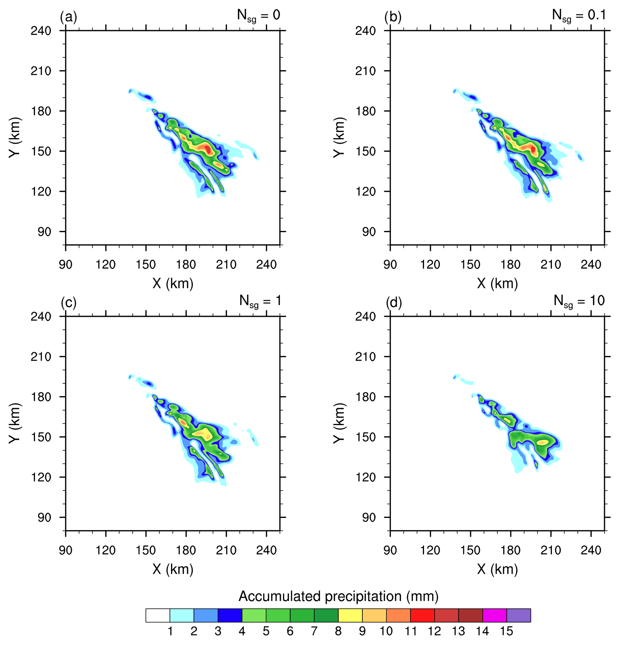
Figure 1 The 4 h accumulated precipitation of the STERAO simulations, where panels (a)–(d) refer to cases with 𝒩_sg=0.0, 0.1, 1.0, and 10.0 ice fragments per collision, respectively. The plots are for a fraction of the computational domain.

3 Simulation of a three-dimensional deep convective case

The test case is illustrated by idealized numerical simulations of the 10 July 1996 thunderstorm in the STERAO (Dye et al., 2000). This case is characterized by a multicellular storm which becomes supercellular after 2 h. The simulations were initialized with the sounding over northeastern Colorado given in Skamarock et al. (2000) and convection was triggered by three 3 K buoyant bubbles aligned along the main diagonal of the X,Y plane along the wind axis. Meso-NH was run for 5 h over a domain with 320×320 grid points and 1 km horizontal grid spacing. There were 50 unevenly spaced vertical levels up to a height of 23 km. With the exception of the wind components advected with a fourth-order scheme, all the fields, including microphysics, were transported by an accurate, conservative, positive-definite piecewise parabolic method scheme (Colella and Woodward, 1984). There were no surface fluxes. The 3-D turbulence scheme of Meso-NH was used. Open lateral boundary conditions were imposed. The upper level damping layer of upward moving gravity waves started above 12 500 m.

Table 1 Background CCN and IFN configuration for the STERAO idealized case simulations.

Figure 2 As in Fig. 1 but for the “RANDOM” simulation.

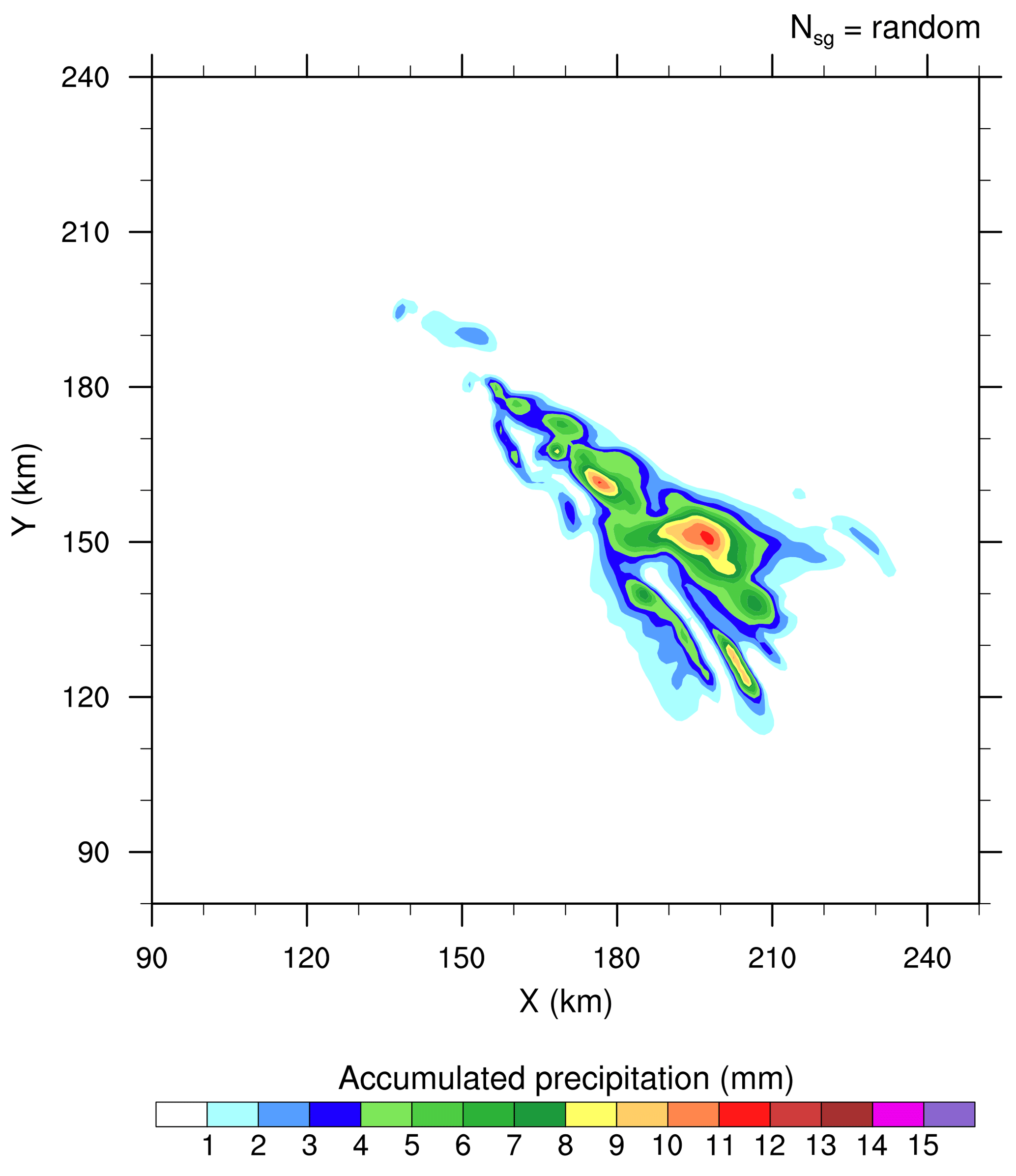
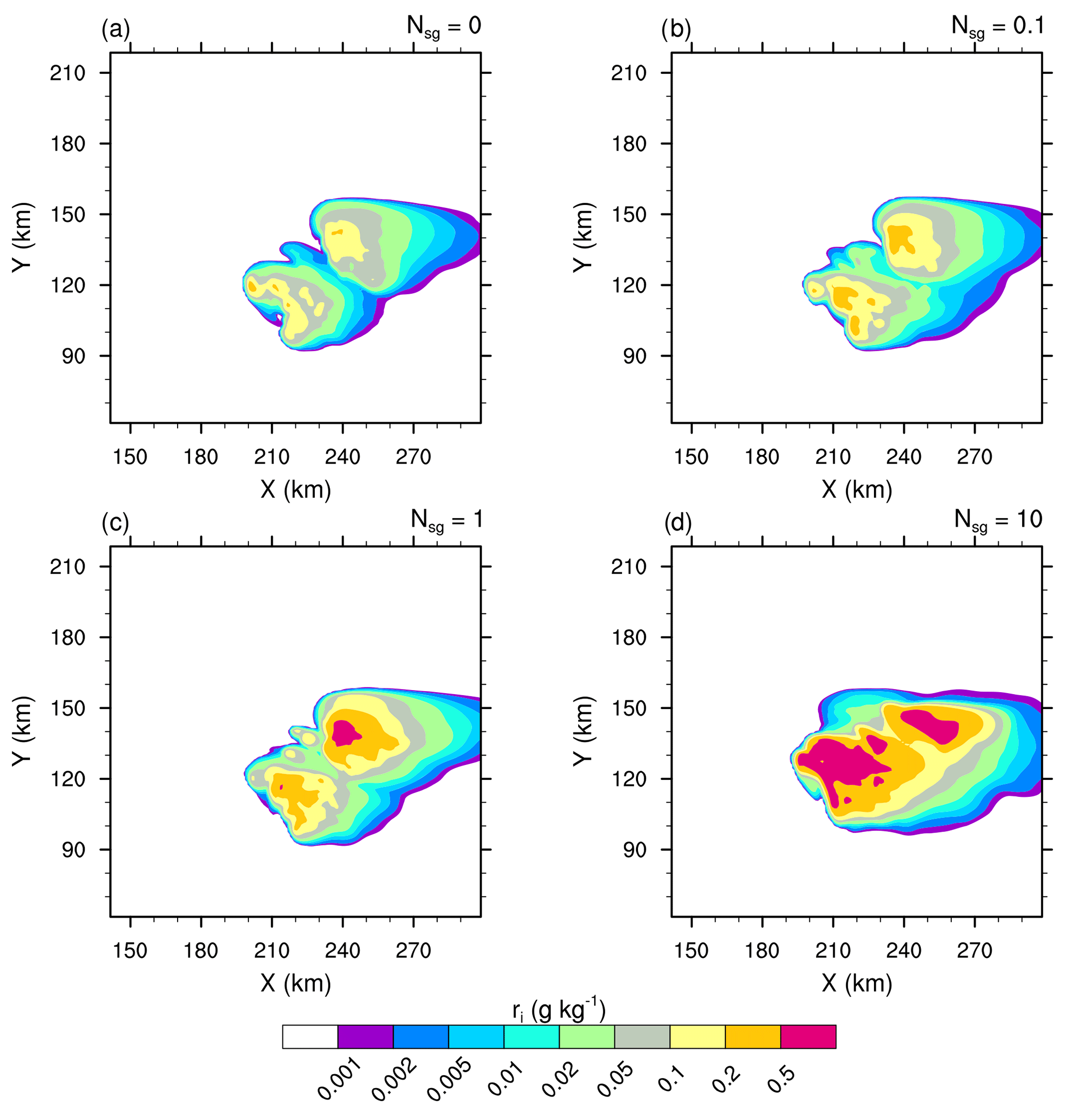
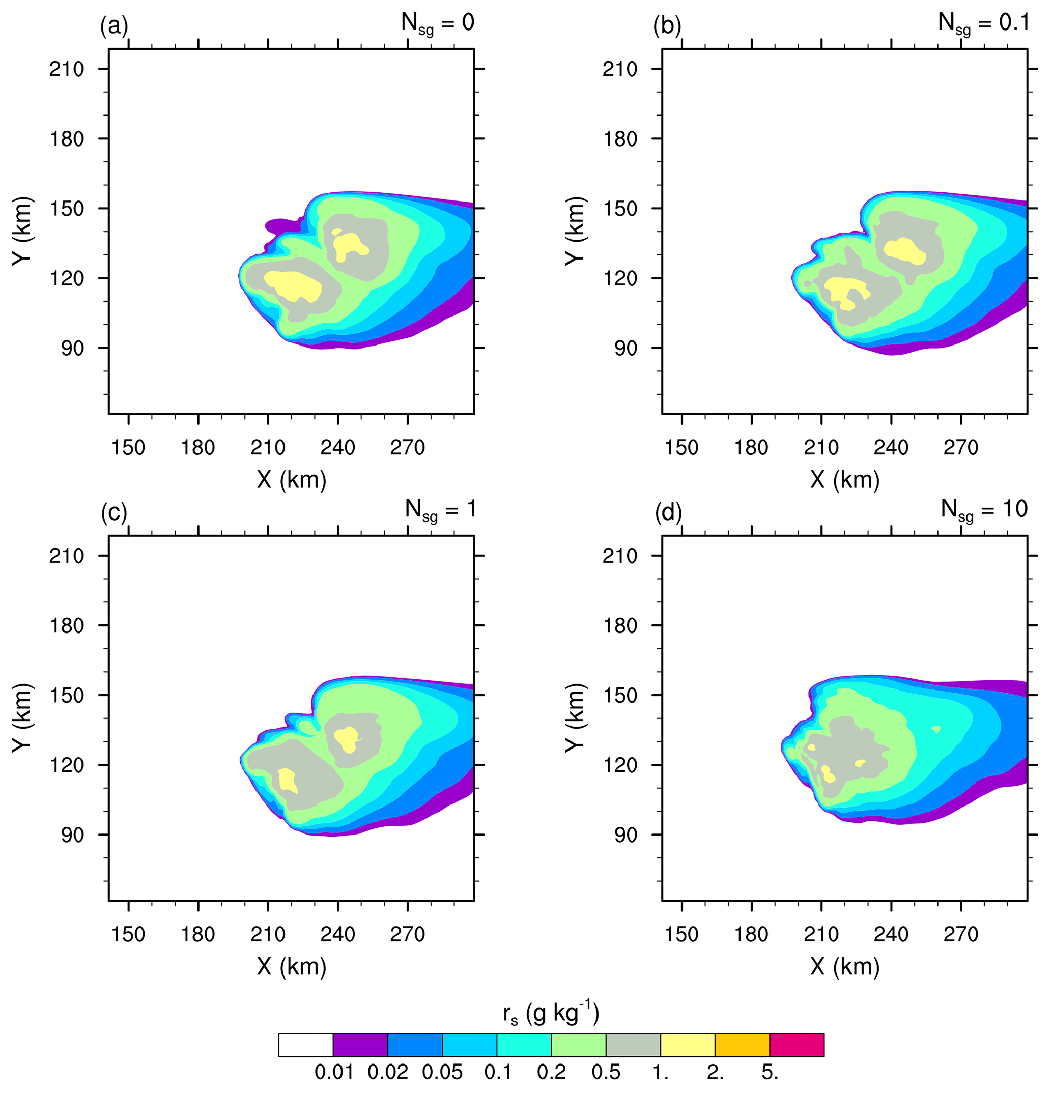
Figure 3 Mixing ratios of the cloud ice (r_i in log scale) of the STERAO simulations at 12 km height, where panels (a)–(d) refer to cases with 𝒩_sg=0.0, 0.1, 1.0, and 10.0 ice fragments per collision, respectively. The plots are for a fraction of the computational domain.

The aerosols were initialized as for the simulated squall-line case studied in Vié et al. (2016). A summary is given in Table 1 for the soluble CCN and for the insoluble IFN. Homogeneous vertical profiles are assumed for the aerosols. Although the LIMA scheme incorporates size distribution parameters and differentiates between the chemical compositions of the CCN and the IFN, the characteristics of the five aerosol modes are standard for the simulations shown here, except for the sensitivity of CIBU to the initial concentration of the IFN which is explored in Sect. 3.5.

Figure 4 As in Fig. 3 but for the mixing ratios of snow aggregates (r_s).

3.1 Impact on precipitation

Figure 1 shows the accumulated precipitation at ground level after 4 h of simulation for the four experiments corresponding to 𝒩_sg=0.0, 0.1, 1.0, and 10.0. The highest amount of rainfall is obtained when the CIBU process is ignored (𝒩_sg=0.0) in Fig. 1a. Then, by increasing the CIBU efficiency 10-fold from 𝒩_sg=0.1, Fig. 1b–d clearly show a steady reduction of precipitation and a fine-scale modification of the precipitation pattern. Furthermore, Fig. 1d reveals that the spread of the precipitation field, caused by the motion of the multicellular storm, is significantly reduced when 𝒩_sg=10.0. The results of Fig. 1 suggest empirically that a plausible range for 𝒩_sg is between 0.1 and 10.0 fragments per collision. A value lower than 0.1 leads to a negligible effect of CIBU in the simulation, while taking 𝒩_sg>10.0 has an excessive impact on the storm rainfall (the “𝒩_sg=50.0” case is not shown). In addition, Fig. 2 shows the results of a simulation, called “RANDOM” hereafter, where ${\mathcal{N}}_{\text{sg}}\in [\mathrm{0.1},\mathrm{10}]$ is generated by a random process as explained above. The perturbation caused by CIBU is also noticeable in this case; it remains weak for the precipitation field. These first 3-D numerical experiments show that inclusion of CIBU can modify surface precipitation strongly when 𝒩_sg>10.0 fragments per aggregate–graupel collision. Taking $\mathrm{0.1}<{\mathcal{N}}_{\text{sg}}<\mathrm{10.0}$ and also considering 𝒩_sg as determined from a random process seems to be a more satisfactory approach. Admittedly, 𝒩_sg∼10 is more than an order of magnitude but our conclusion is to recommend an upper bound value of 𝒩_sg that is much lower than the former N=50 used by Yano and Phillips (2011) with their notation in the box model.

3.2 Changes in the microphysics

Essentially, intensifying the CIBU process by increasing 𝒩_sg leads to higher cloud ice crystal concentrations which deplete the supersaturation of water vapour that would otherwise contribute to the deposition growth of the snow aggregates. However, a further effect is possible because the partial mass sink of the snow aggregate particles also slows down the flux of graupel particles, which form essentially by heavy riming and conversion of the snow aggregates. This point is now examined by considering the ice in the high levels of the STERAO cells. Figures 3–5 reproduce the 10 min average of the mixing ratios r_i, r_s, and r_g at 12 km from the four experiments having 𝒩_sg=0.0, 0.1, 1.0, and 10.0 after 4 h. The increase of the cloud ice mixing ratio with 𝒩_sg is clear in the area covered by the 0.2 g kg⁻¹ isocontour in Fig. 3. Simultaneously, a slight decrease of r_s, indicating a slow erosion of the mass of the aggregates, is visible in Fig. 4. The effect on the graupel (Fig. 5) is even smaller but appears clearly for the case 𝒩_sg=10.0, where less graupel is found. A last illustration is provided in Fig. 6, showing the number concentration of cloud ice N_i at a higher altitude of 15 km. Again, the increase of N_i follows 𝒩_sg with an explosive multiplication of N_i when 𝒩_sg=10.0 (N_i is well above 1000 crystals kg⁻¹ of dry air in this case). Figure 7 summarizes the behaviour of r_i, r_s, and r_g at 12 km height, and of N_i at 15 km height, for the “RANDOM” simulation. A comparison with Figs. 3–6 shows that the results are those expected. The examination of the microphysics fields suggests that the “RANDOM” simulation corresponds to a mean CIBU intensity intermediate between 𝒩_sg=1 and 𝒩_sg=10.

Figure 5 As in Fig. 3 but for the mixing ratios of graupel (r_g).

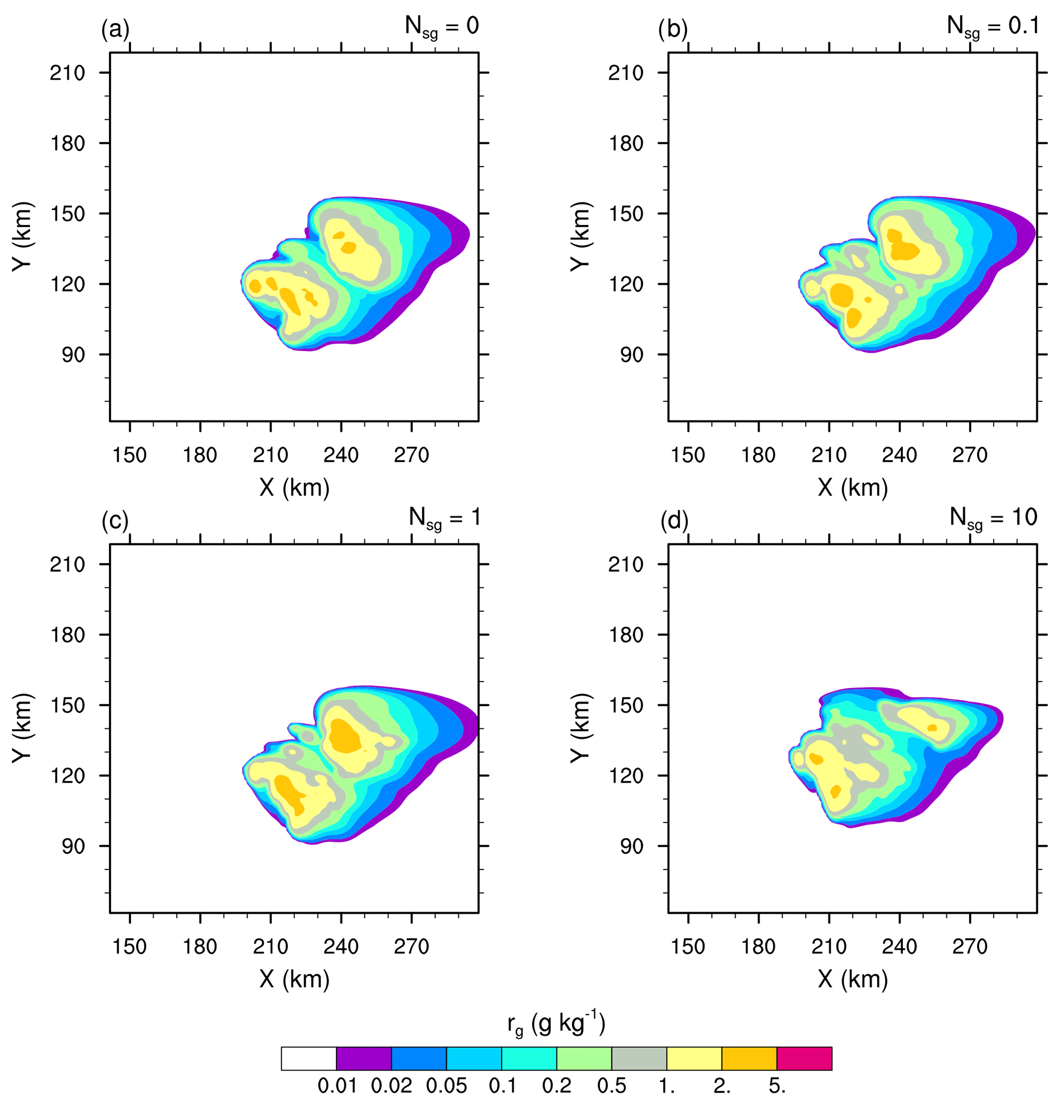
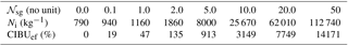
Table 2 After 3 h of simulation, maximum value of the cloud ice number concentration $N_{i_{max}}$ as a function of the number of fragments produced per snow-aggregate–graupel collision 𝒩_sg. The last row shows the CIBU enhancement factor CIBU_ef in percent (see text).

The analysis of the STERAO simulations continues with an examination of the vertical profiles of microphysics budgets. The profiles are 10 min averages of all cloudy columns that contain at least 10⁻³ g kg⁻¹ of condensate at any level. The column selection is updated at each time step because of the evolution and motion of the storm. Figure 8 shows the mixing ratio profiles for three cases: 𝒩_sg=0.0, “RANDOM”, and 𝒩_sg=10.0. A key feature that shows up in Fig. 8a–c is the increase of the r_i peak value at 11 km altitude. This change is accompanied by a reduction of r_s (more visible between Fig.  8b and c) and by a reduction of r_g, which stands out at z=8000 m. The decrease of r_g, even when graupel is a passive collider for CIBU, is the result of the decrease of r_s in the growth chain of the precipitating ice. The low value of the mean r_r profiles, compared to the mixing ratios of the ice phase above, is explained by the fact that rain is spread over fewer grid points than the ice in the anvil is (the mixing ratio profiles are averaged over the same number of columns).

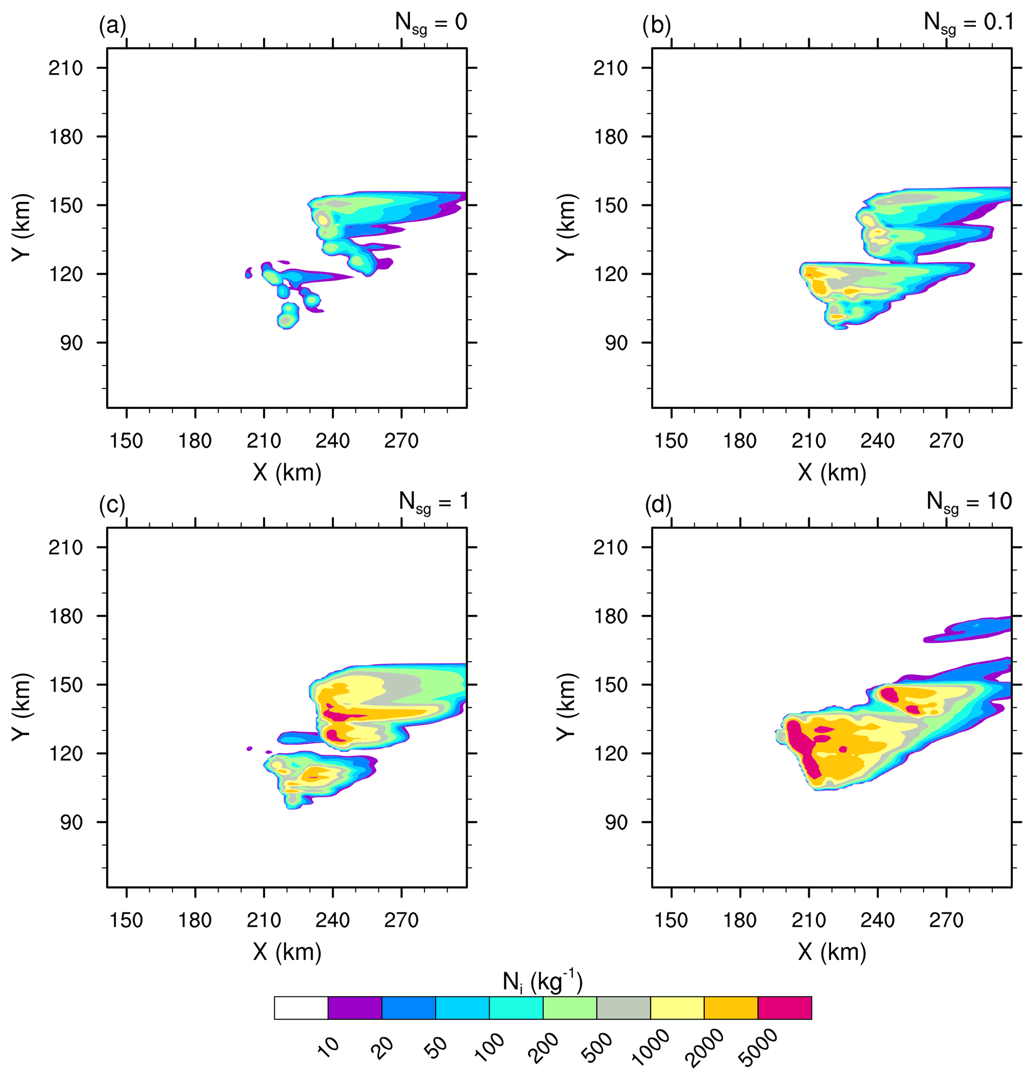
Figure 6 Number concentration of the cloud ice (N_i in log scale) of the STERAO simulations at 15 km height, where panels (a)–(d) refer to cases with 𝒩_sg=0.0, 0.1, 1.0, and 10.0 ice fragments per collision, respectively. The plots are for a fraction of the computational domain.

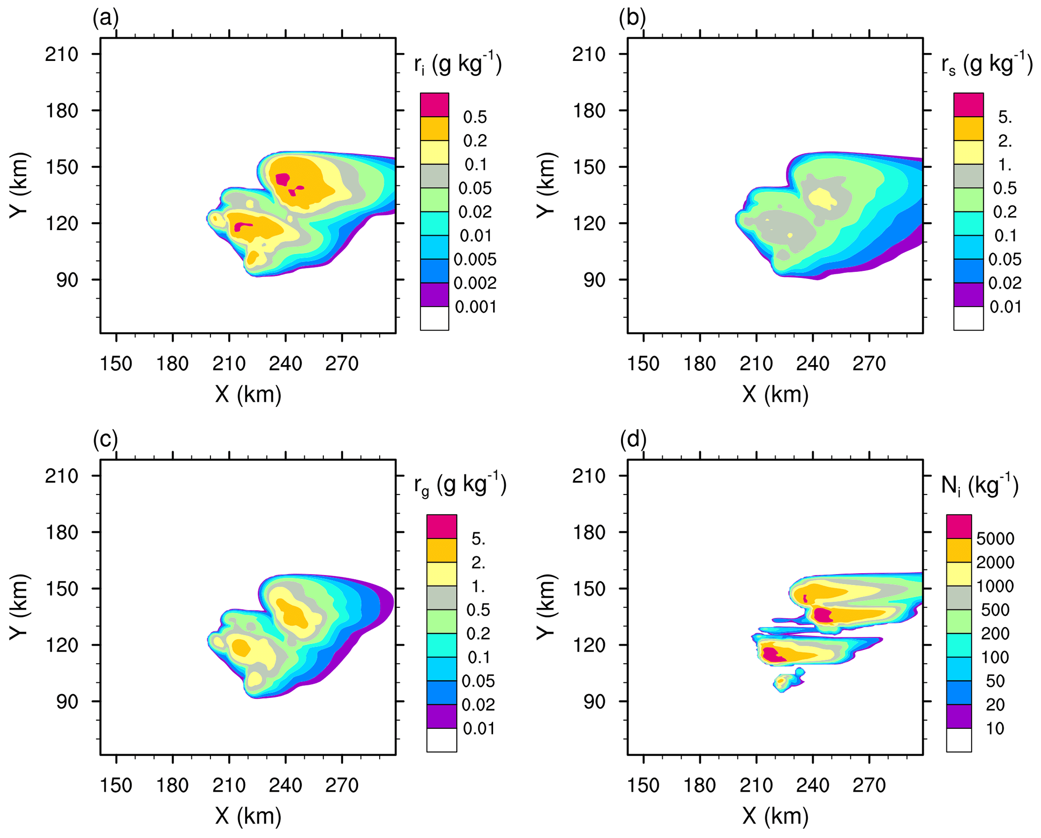
Figure 7 “RANDOM” case of the STERAO simulations showing the mixing ratios of (a) the cloud ice (r_i), (b) the snow aggregates (r_s), and (c) the graupel (r_g) at 12 km height. Panel (d) refers to the number concentration of the cloud ice crystals (N_i) at 15 km height. The plots are for a fraction of the computational domain.

3.3 Budget of ice mixing ratios

This step is devoted to the microphysics tendencies (using 10 min average again with the nomenclature of the processes provided in Table 3) of the ice mixing ratios in Figs. 9–11 to assess the impact of the CIBU process. We do not discuss the case of the liquid phase here because the tendencies (not shown) are only marginally affected by the CIBU process.

As expected, many tendencies of r_i (Fig. 9a–c) are affected by the CIBU process. The main processes standing out in Fig. 9a, when CIBU is not activated, are CEDS (deposition–sublimation), essentially a gain term, and AGGS (aggregation), the main loss of r_i by aggregation with a rate of $\mathrm{0.5}\times {\mathrm{10}}^{-\mathrm{3}}$ $\mathrm{g}{\mathrm{kg}}^{-\mathrm{1}}{\mathrm{s}}^{-\mathrm{1}}$. The loss of r_i by CFRZ (drop freezing by contact) makes a moderate contribution as some raindrops are present in the glaciated part of the storm. Above z=10 000 m, the net loss of r_i (AGGS and SEDI, the cloud ice sedimentation) is balanced by the convective vertical transport (not shown). When 𝒩_sg= RANDOM, the r_i tendencies are amplified, even with a modest contribution of $\sim \mathrm{0.2}\times {\mathrm{10}}^{-\mathrm{3}}$ $\mathrm{g}{\mathrm{kg}}^{-\mathrm{1}}{\mathrm{s}}^{-\mathrm{1}}$ for CIBU itself. The growth of AGGS, which doubles at 10 km height, is caused by CIBU and by an increase in the convection because SEDI (a loss at this height) is amplified in response to an increase of r_i in the upper levels. The CFRZ contribution is also increased. The last case, with 𝒩_sg=10 (Fig. 9c), confirms a further increase of the rates except for CFRZ, interpreted here as a lack of raindrops.

The budget of the snow-aggregate mixing ratio in Fig. 10 contains many processes of equivalent importance in the range $\pm \mathrm{0.05}\times {\mathrm{10}}^{-\mathrm{3}}$ $\mathrm{g}{\mathrm{kg}}^{-\mathrm{1}}{\mathrm{s}}^{-\mathrm{1}}$ but SEDS (sedimentation of snow aggregates) dominates at z=11 000 m and at z=7000 m. The inclusion of CIBU (Fig. 10b–c) mostly leads to an increase of AGGS, and the other processes remaining almost the same. Finally, many processes contribute to the evolution of the graupel mixing ratio profiles (Fig. 11). The strongest loss is in the GMLT term (melting of graupel) that converts graupel into rain (down to $-\mathrm{0.3}\times {\mathrm{10}}^{-\mathrm{3}}$ $\mathrm{g}{\mathrm{kg}}^{-\mathrm{1}}{\mathrm{s}}^{-\mathrm{1}}$) while CFRZ reaches $\mathrm{0.15}\times {\mathrm{10}}^{-\mathrm{3}}$ $\mathrm{g}{\mathrm{kg}}^{-\mathrm{1}}{\mathrm{s}}^{-\mathrm{1}}$. The sedimentation term SEDG (sedimentation of graupel) lies between $-\mathrm{0.3}\times {\mathrm{10}}^{-\mathrm{3}}$ $\mathrm{g}{\mathrm{kg}}^{-\mathrm{1}}{\mathrm{s}}^{-\mathrm{1}}$ at z=10 000 m and $\mathrm{0.15}\times {\mathrm{10}}^{-\mathrm{3}}$ $\mathrm{g}{\mathrm{kg}}^{-\mathrm{1}}{\mathrm{s}}^{-\mathrm{1}}$ at 5000 m. Another noticeable effect is the sign change of DEPG (growth of graupel by deposition, $\pm \mathrm{0.07}\times {\mathrm{10}}^{-\mathrm{3}}$ $\mathrm{g}{\mathrm{kg}}^{-\mathrm{1}}{\mathrm{s}}^{-\mathrm{1}}$) showing that the water vapour is supersaturated above z=7000 m and undersaturated below z=7000 m on average. The relative importance of these processes does not change very much when CIBU is increased but all tendencies weaken. To sum up, the impact of CIBU is modest for the microphysics mixing ratios. The increase of ice fragments in r_i is approximately compensated by an increase of AGGS (see Figs. 9 and 10).

Table 3 Nomenclature of the microphysics processes of the budget profiles.

3.4 Budget of cloud ice concentration

This subsection examines the behaviour of the cloud ice number concentration as a function of the strength of the CIBU process after 4 h of simulation. Figure 12 shows that the altitude of the N_i peak value decreases when 𝒩_sg increases. In the absence of CIBU (𝒩_sg=0), the source of N_i is the heterogeneous nucleation processes on insoluble IFN and on coated IFN (nucleation by immersion) which are more efficient at low temperature. Nucleation on IFN provides a mean peak value N_i=400 kg⁻¹ at z=11 500 m. In contrast, the 𝒩_sg=10 case (here scaled by a factor 0.1 for ease of reading) keeps the trace of an explosive production of cloud ice concentration, N_i=7250 kg⁻¹, due to CIBU. The altitude of the maximum of N_i in this case (z=10 000 m) is consistent with the location of the maximum value of the r_s×r_g product (see Fig. 8). The “RANDOM” simulation produces N_i=1100 kg⁻¹ at z=11 000 m, a number concentration similar to that found for the 𝒩_sg=2 case. Table 2 reports the peak amplitude of the N_i profiles as a function of 𝒩_sg but after 3 h of simulation, when the CIBU rate is strongly dominant. Additional cases were run to cover $\mathrm{0.1}<{\mathcal{N}}_{\text{sg}}<\mathrm{50}$ with a logarithmic progression above 𝒩_sg=1.0. The CIBU enhancement factor, CIBU_ef, was computed as $N_{\text{i}}\left({\mathcal{N}}_{\text{sg}}\right)/N_{\text{i}}({\mathcal{N}}_{\text{sg}}=\mathrm{0})-\mathrm{1}$ since N_i(𝒩_sg=0) constitutes a baseline not affected by CIBU. The results presented in Table 2 show that the growth of N_i is fast when 𝒩_sg reaches ∼5 (CIBU_ef rises sharply from 135 % to 913 % when 𝒩_sg increases from 2 to 5). Taking 𝒩_sg=50 leads to an extremely high peak value of N_i.

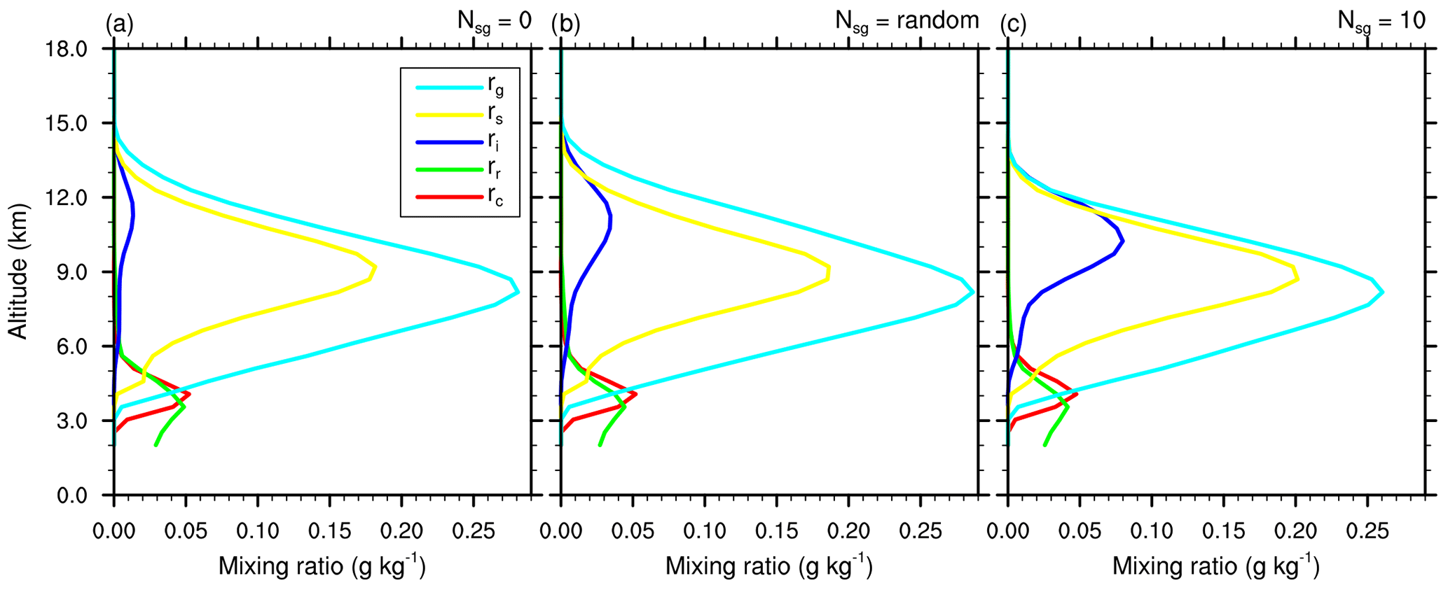
Figure 8 Mean profiles of condensate mixing ratios r_c, r_r, r_i, r_s, and r_g (in g kg⁻¹) of the STERAO simulations corresponding to (a) the 𝒩_sg=0.0 case, (b) the “RANDOM” case, and (c) the case with 𝒩_sg=10.0.

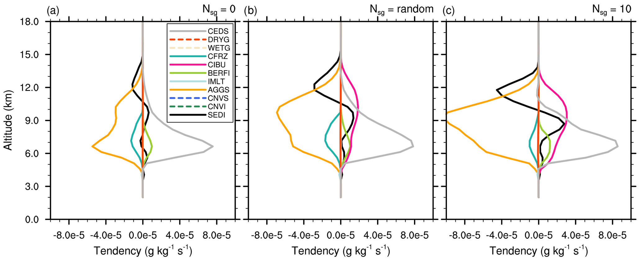
Figure 9 Mean microphysics profiles of cloud ice mixing ratio tendencies of the STERAO simulations corresponding to (a) the 𝒩_sg=0.0 (no CIBU) case, (b) the “RANDOM” case, and (c) the case with 𝒩_sg=10.0. The dashed lines are associated with processes having no significant impact on these budgets.

The N_i tendencies are the subject of Fig. 13. Many processes are involved during the temporal integration of N_i. The 𝒩_sg=0 case confirms the importance of the heterogeneous nucleation process by deposition (HIND; see Table 3) and, to a lesser degree, by immersion (HINC) at 8 km height. HIND peaks at three altitudes with two sources of IFN (Table 1). This case also reveals the importance of the HMG (Hallett–Mossop on graupel, 1.3 ${\mathrm{kg}}^{-\mathrm{1}}{\mathrm{s}}^{-\mathrm{1}}$) and HMS (Hallett–Mossop on snow, 0.85 ${\mathrm{kg}}^{-\mathrm{1}}{\mathrm{s}}^{-\mathrm{1}}$) processes. Here, we consider that H–M also operates for the snow aggregates because this category of ice includes lightly rimed particles that can rime further to form graupel particles. These processes are first compensated by AGGS (capture of cloud ice by the aggregates). There is also a loss of cloud ice due to CFRZ and CEDS with the full sublimation of individual cloud ice crystals which replenish the IFN reservoir. The sedimentation profile transports ice from the cloud top (SEDI < 0) to mid-level cloud (SEDI > 0). Then, taking 𝒩_sg= RANDOM shows the domination of the CIBU process, which reaches 2.5 ${\mathrm{kg}}^{-\mathrm{1}}{\mathrm{s}}^{-\mathrm{1}}$ at 5 km height. The enhancement of HIND at cloud top can also be noted. The CIBU source of ice crystals is balanced by an increase of AGGS and, above all, of CEDS (here, CEDS represents the sublimation of the ice crystal concentration when the crystals are detrained in the low level of the cloud vicinity, such as below the anvil). Finally, the 𝒩_sg=10 case demonstrates the reality of the exponential-like growth of N_i because the three main driving terms (CIBU, CEDS, and AGGS) are growing at a similar rate, which is multiplied by a factor of approximately 5.

Figure 10 As in Fig. 9 but for snow aggregates.

Figure 11 As in Fig. 9 but for graupel.

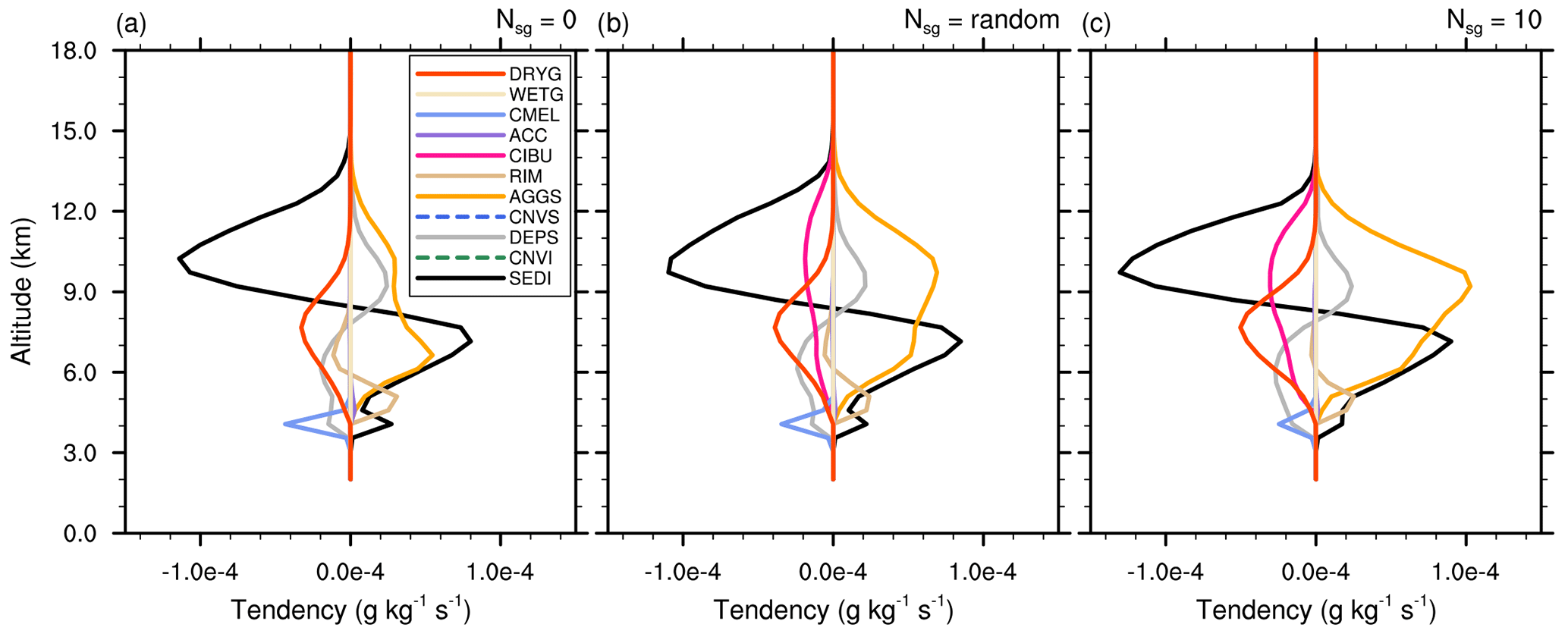
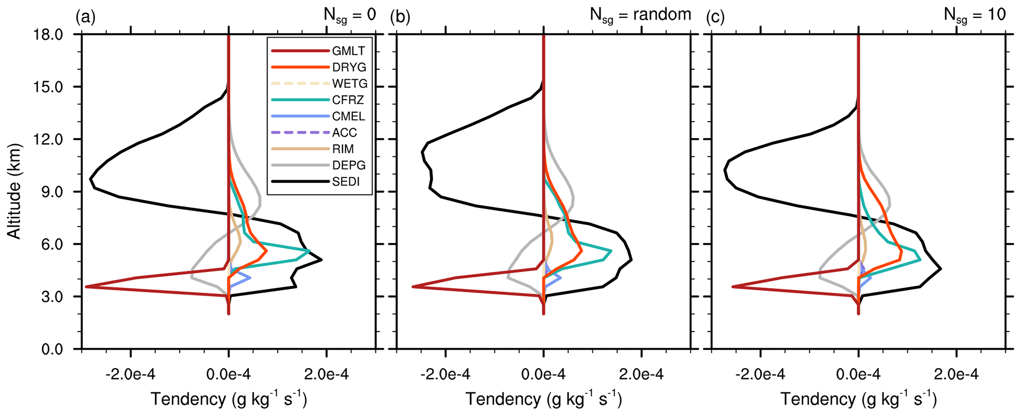
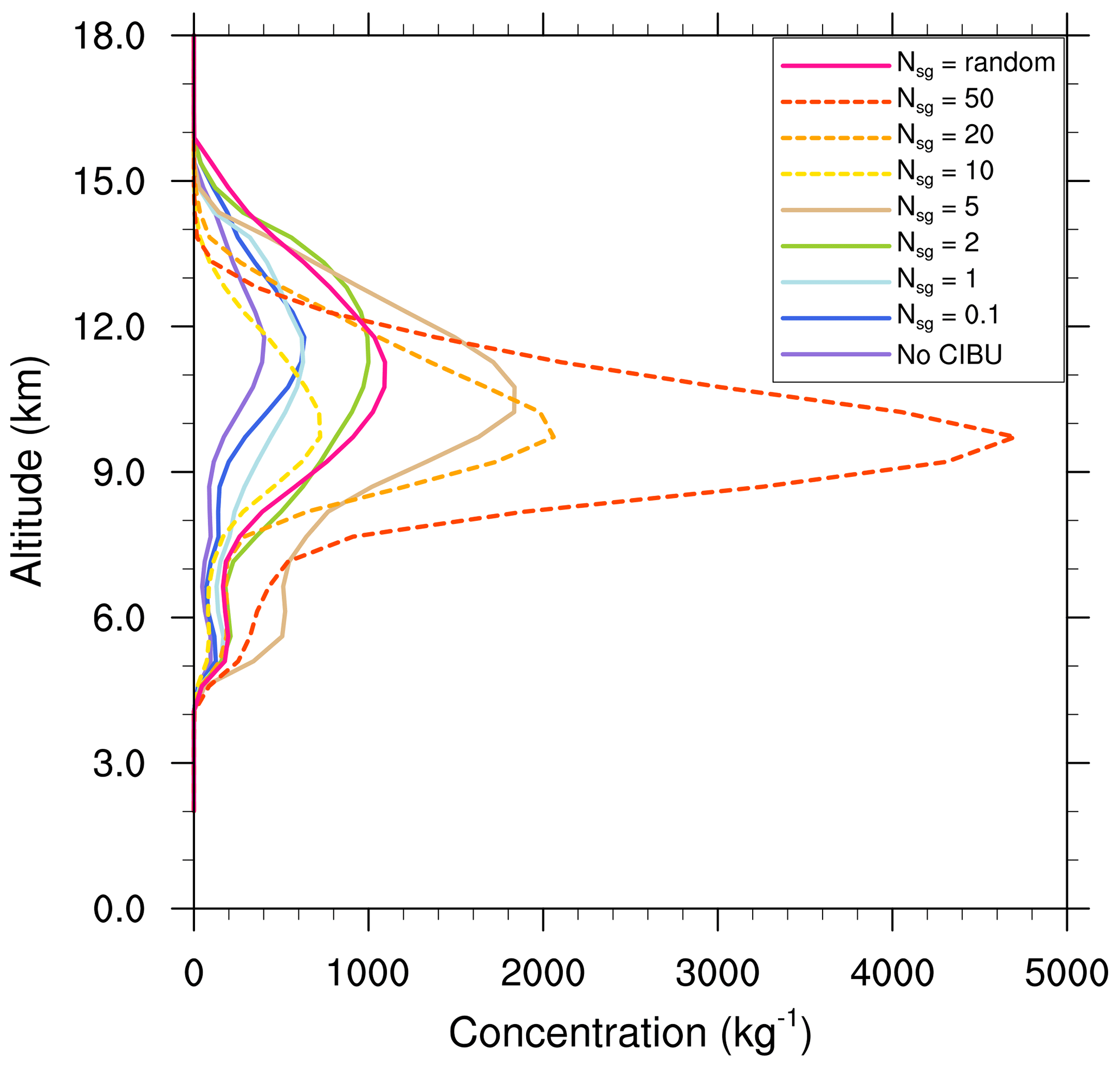
Figure 12 Mean profiles of the cloud ice crystal concentrations N_i (g kg⁻¹) of the STERAO simulations corresponding to different values of 𝒩_sg (see the legend for details). The profiles drawn with a dashed line have been divided by 10 to fit into the plot.

3.5 Sensitivity to the initial concentration of freezing nuclei

The purpose of the last series of experiments was to look more closely at the sensitivity of the cloud ice concentration to N_IFN, the initial concentration of the IFN. Numerical simulations were run with N_IFN decreasing 10-fold from 100 to 0.001 day m⁻³ for each IFN mode (see Table 1). Two different cases were considered. In the first case, CIBU was activated with the RANDOM set-up while, in the second case, CIBU effects were ignored. All the results are summarized in the plots of Fig. 14.

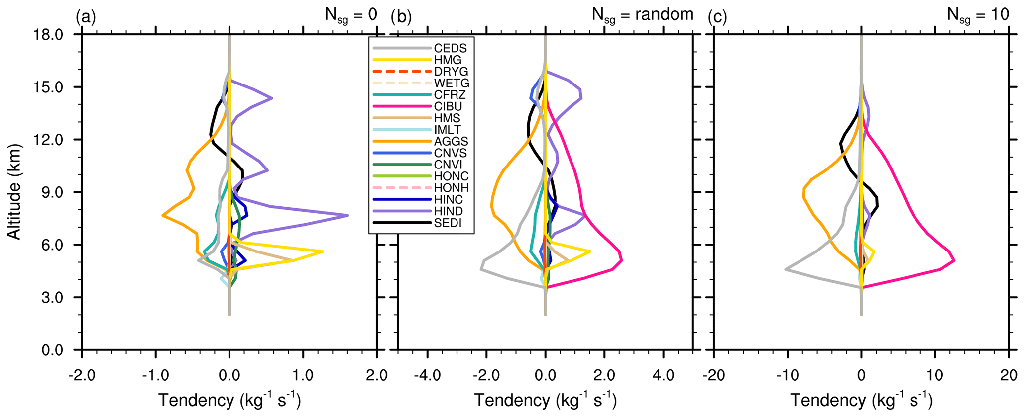
Figure 13 Mean microphysics profiles of the cloud ice crystal concentration tendencies of the STERAO simulations corresponding to (a) the 𝒩_sg=0.0 (no CIBU) case, (b) the “RANDOM” case, and (c) the case with 𝒩_sg = 10.0 (note that the horizontal scale increases from panel a to panel c). The dashed lines of the list box are associated with processes having no significant impact on these budgets.

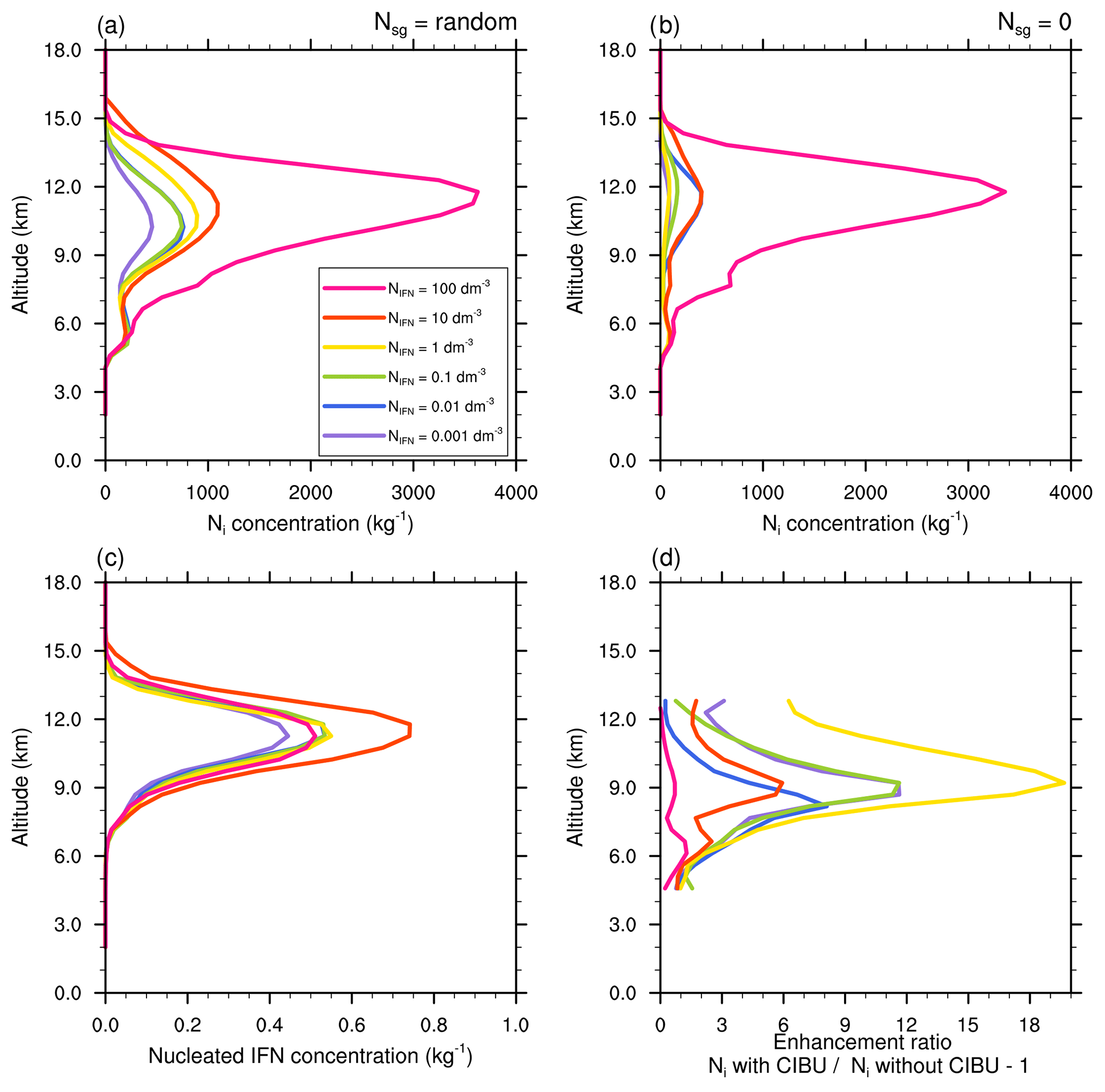
Figure 14 Mean profiles of cloud ice crystal concentration for initial IFN concentrations from 100 to 0.001 day m⁻³ of the STERAO simulations corresponding to (a) the CIBU simulation and “RANDOM” case and (b) the non-CIBU simulation. The mean profiles of the nucleated IFN concentrations are plotted in panel (c) after rescaling to fit the [0.0, 1.0] range. The rough estimate of CIBU enhancement factor of N_i is plotted in panel (d) as a function of the initial IFN concentrations.

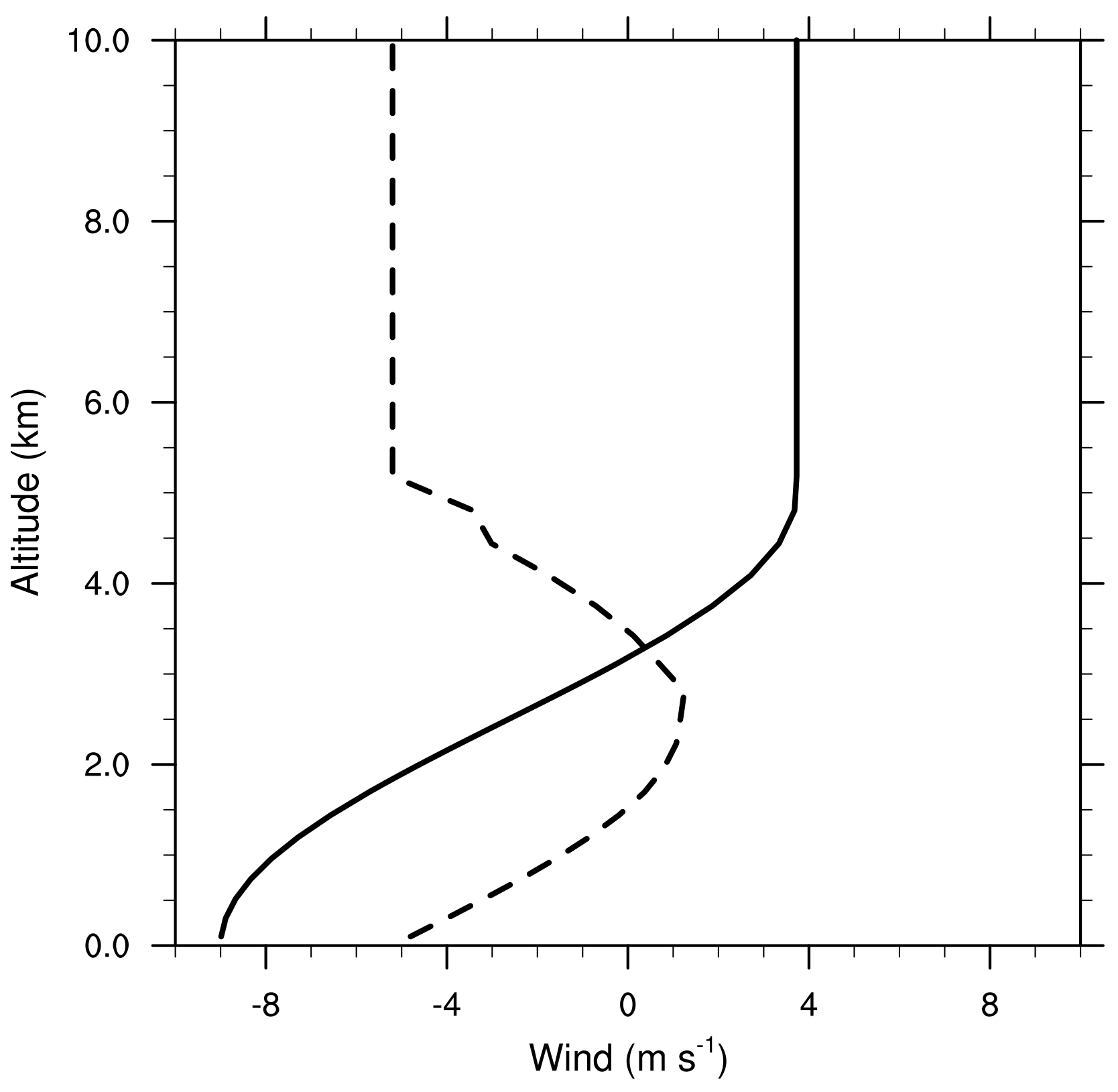
Figure 15 Vertical profile of the horizontal wind components of the WK84 simulations. The solid line with a constant shear ($\mathrm{2.5}\times {\mathrm{10}}^{-\mathrm{2}}$ s⁻¹) refers to U, the x component of the wind, and the dashed line with a jet-like structure refers to V, the y component of the wind. U and V are constant above 5 km height.

Figure 14a shows that N_i concentrations did not change very much for a wide range of N_IFN concentrations, which were varied 10-fold. This clearly illustrates the predominance of the CIBU effect for current IFN concentrations, which disconnects N_i concentrations from the underlying abundance of IFN particles. Likewise, the small hump superimposed on all profiles at 5000 m height reveals a residual effect of the Hallett–Mossop process. Another remarkable feature is that a fairly low IFN concentration (N_IFN=0.001 day m⁻³) suffices to initiate the CIBU process and to reach N_i∼500 kg⁻¹. In contrast, and in the absence of CIBU (Fig. 14b), the N_i profiles show a sensitivity to IFN nucleation that is, indeed, difficult to interpret because of the non-monotonic trend of the N_i profiles with respect to N_IFN. Some insight can be gained by checking the concentration of the nucleated IFN of the first IFN mode (dust particles). In Fig. 14c, the IFN profiles are rescaled (multiplication by an appropriate number of powers of 10) to be comparable. This is equivalent to computing an IFN nucleation efficiency. The important result here is that the number of nucleated IFN evolves in close proportion to the initially available IFN concentrations, meaning that, as expected, the nucleating properties of the IFN do not depend on the IFN concentration. The last plot (Fig. 14d) reproduces the normalized differences of N_i profiles between twin simulations performed with and without CIBU. Although simulations using the same initial concentration N_IFN may diverge because of additional non-linear effects (vertical transport, enhanced or reduced cloud ice sink processes), the figure gives an indication of the bulk sensitivity of CIBU to the IFN. The enhancement ratio due to CIBU remains low (less than 1 for N_IFN∼100 day m⁻³) but can reach a factor of 20 at 9000 m height in the case of moderate IFN concentration, i.e. N_IFN∼1 day m⁻³. The behaviour of LIMA can be explained in the sense that increasing N_IFN too much leads to smaller pristine crystals that need a longer time to grow before being included in the next category of snow aggregates because such inclusion is size-dependent (see Harrington et al., 1995, and Vié et al., 2016). On the other hand, a low concentration of N_IFN initiates fewer snow aggregates and thus fewer graupel particles, so the whole CIBU efficiency is also reduced. Consequently, this study confirms the essential role of CIBU in compensating for IFN deficit when cloud ice concentrations are increasing.

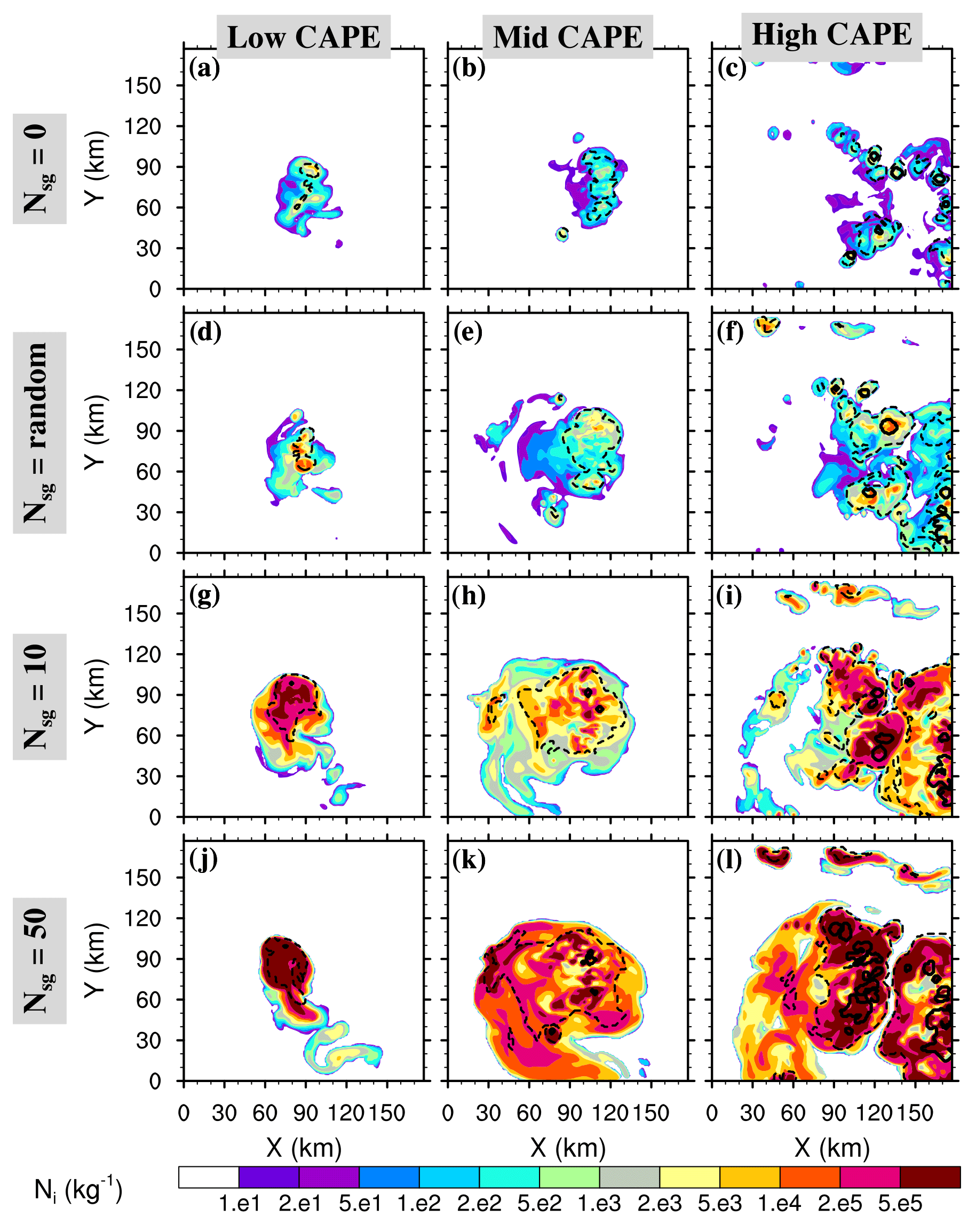
Figure 16 Small ice concentration N_i average between 9.5 and 10.5 km height after 4 h of the WK84 simulations, where panels (a–c) refer to no CIBU cases (𝒩_sg=0.0), (d–f) to cases with random CIBU ($\mathrm{0.1}<{\mathcal{N}}_{\text{sg}}<\mathrm{10}$), (g–i) to cases with a high CIBU effect (𝒩_sg=10.0), and (j–l) to cases with an intense CIBU effect (𝒩_sg=50.0). The contours are the cloud top heights with dotted lines for 11 km and solid lines for 13 km.

4 Simulation of a three-dimensional idealized supercell storm with varying atmospheric stability

The idealized sounding of Weisman and Klemp (1982, 1984) was appealing to use for this test case (referred to as WK) because the intensity of the CAPE can be easily modified by changing a reference water vapour mixing ratio. The environmental conditions of the simulations were close to those of the STERAO case with the same set-up for the physics and the aerosol characteristics. The simulation domain was 180×180 grid points at 1 km resolution and 70 levels with a mean vertical grid spacing of 350 m. Convection was triggered by a domain-centred single 2 K buoyant air parcel of 10 km radius and 3 km height. The base of the upper level Rayleigh damper was set at 15 km above ground level.

Meso-NH was initialized with the analytic sounding of Weisman and Klemp (1984) with low two-dimensional shear. The hodograph in Fig. 15 features a three-quarter cycle with a constant wind of 6.4 m s⁻¹ (in modulus) above the height of 5 km. When running Meso-NH, a constant translation speed (U_trans=5 m s⁻¹ and V_trans=1 m s⁻¹) was added to the wind to keep the convection well centred in the domain of simulation. As explained in Weisman and Klemp (1982), buoyancy was varied by altering the magnitude of the surface water vapour mixing ratio q_v0 keeping with the Weisman and Klemp (1984) notation. Three water vapour profiles were defined by taking q_v0=13.5 g kg⁻¹, hereafter the “low” CAPE case of 1970 J kg⁻¹, q_v0=14.5 g kg⁻¹ as the “mid” CAPE case of 2400 J kg⁻¹, and q_v0=15.5 g kg⁻¹ as the “high” CAPE case of 2740 J kg⁻¹. Four experiments of 4 h each were performed for each CAPE case by using different magnitudes of 𝒩_sg.

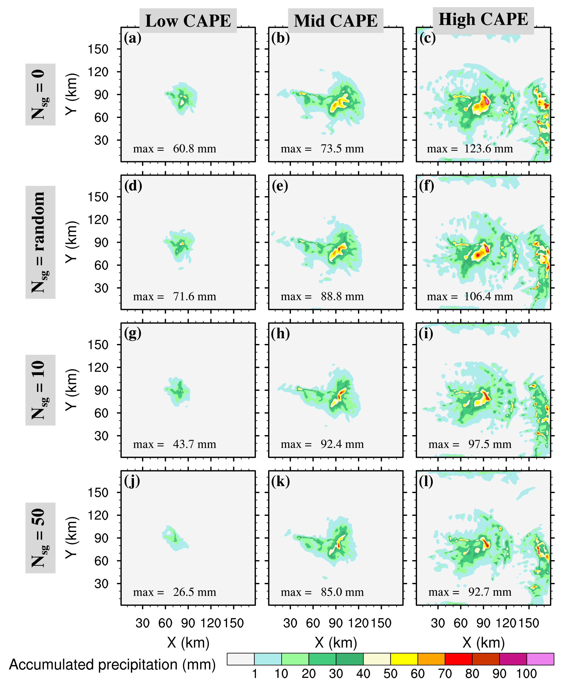
Figure 17 As in Fig. 16 but for the 4 h accumulated precipitation of the WK84 simulations. The peak value (max in millimetres) corresponds to the peak value of precipitation of the main convective clouds in the centre of the simulation domain.

4.1 Sensitivity to mean ice concentrations

Figure 16 shows the mean concentrations of small ice crystals between 9.5 and 10.5 km levels plotted on a log scale after 4 h of simulation. In addition, two cloud top height (CTH) contours delineate the 11 km (dotted line) and 13 km (solid line) levels. The 𝒩_sg=0, RANDOM, 10, and 50 cases, are explored for each sounding (“low”, “mid”, and “high” CAPE). In the absence of CIBU (first row in Fig. 16), the cloud ice concentrations N_i are in the range of what was simulated for the STERAO case (see Figs. 6 and 7d). The N_i peak values do not increase with the initial CAPE (Fig. 16a, b) but the area of CTH > 11 km is larger in the “mid” CAPE case. The “high” case is a little bit more difficult to analyse because of earlier development of the convection, spreading out ahead of the main system. This shows up in the “low” and “mid” CAPE cases but the N_i peak values of the “high” CAPE case are in the same range as for the “low” CAPE case, meaning that higher environmental instability is not decisive in fixing the N_i peak values. In the 𝒩_sg=10 and 50 cases, we retrieve the dramatic increase of N_i due to increasing CIBU efficiency. The enhancement is locally as high as 1000-fold in the strongest case (𝒩_sg=50). There are also other noteworthy features: an increase of the N_i area coverage with 𝒩_sg (less visible in the “low” CAPE case) and a higher CTH which exceeds 13 km for the “mid” and “high” CAPE cases. All these observations strongly suggest that convection is invigorated when the CIBU effect is increased. In contrast, the simulations run with 𝒩_sg= RANDOM using values taken in the 0.1–10 range (see Sect. 2.1), show a moderate effect of CIBU. Locally, N_i values reach 1×10⁴ kg⁻¹, which is 100 times lower than N_i peak values in the 𝒩_sg=50 cases but approximately 10 times higher than in the “no CIBU” case (𝒩_sg=0). Finally, the simulation results suggest that the 𝒩_sg parameter could be constrained by satellite data because of the sensitivity of CIBU to the cloud ice coverage and the cloud top height.

Figure 18 As in Fig. 16 but for the total ice thickness in millimetres after 4 h of the WK84 simulations. The contours are the small ice thickness component (THIC) taken at 1 mm. The peak value of THIC (THIC_max) is given in millimetres.

4.2 Sensitivity to precipitation

The 4 h accumulated precipitation maps are presented in Fig. 17. On each row, precipitation increases from the “low” to “high” CAPE cases. This is because the CAPE is enhanced by the addition of more water vapour. Looking at the sensitivity of the accumulated precipitation to 𝒩_sg, it is not as easy to draw a general conclusion on the decrease of the precipitation peak with 𝒩_sg as for the STERAO case (see Sect. 3.1). The reason is the highly concentrated precipitation field, which leads to a sharp gradient around the location of the peak value. However, the decrease of the precipitation with 𝒩_sg is observed in the “low” and “high” CAPE cases. In the “mid” case, the precipitation peak value remains high when 𝒩_sg=50 but the area where the precipitation is less than 10 mm shrinks continuously. The reduction of the area where the precipitation amount is greater than 10 mm when 𝒩_sg is increased was found in all CAPE cases (not shown).

In conclusion, the simulations illustrate the fact that the precipitation patterns are affected by the value of the 𝒩_sg parameter. When 𝒩_sg is increased from 0 to 50, the precipitation is reduced either for the peak value or at least for the precipitating area. This is consistent with our previous results concerning the STERAO case. The conversion efficiency of the small ice crystals to precipitating ice particles is lower when the cloud ice concentration is high because the deposition growth of individual small crystals is limited by the amount of supersaturated water vapour available.

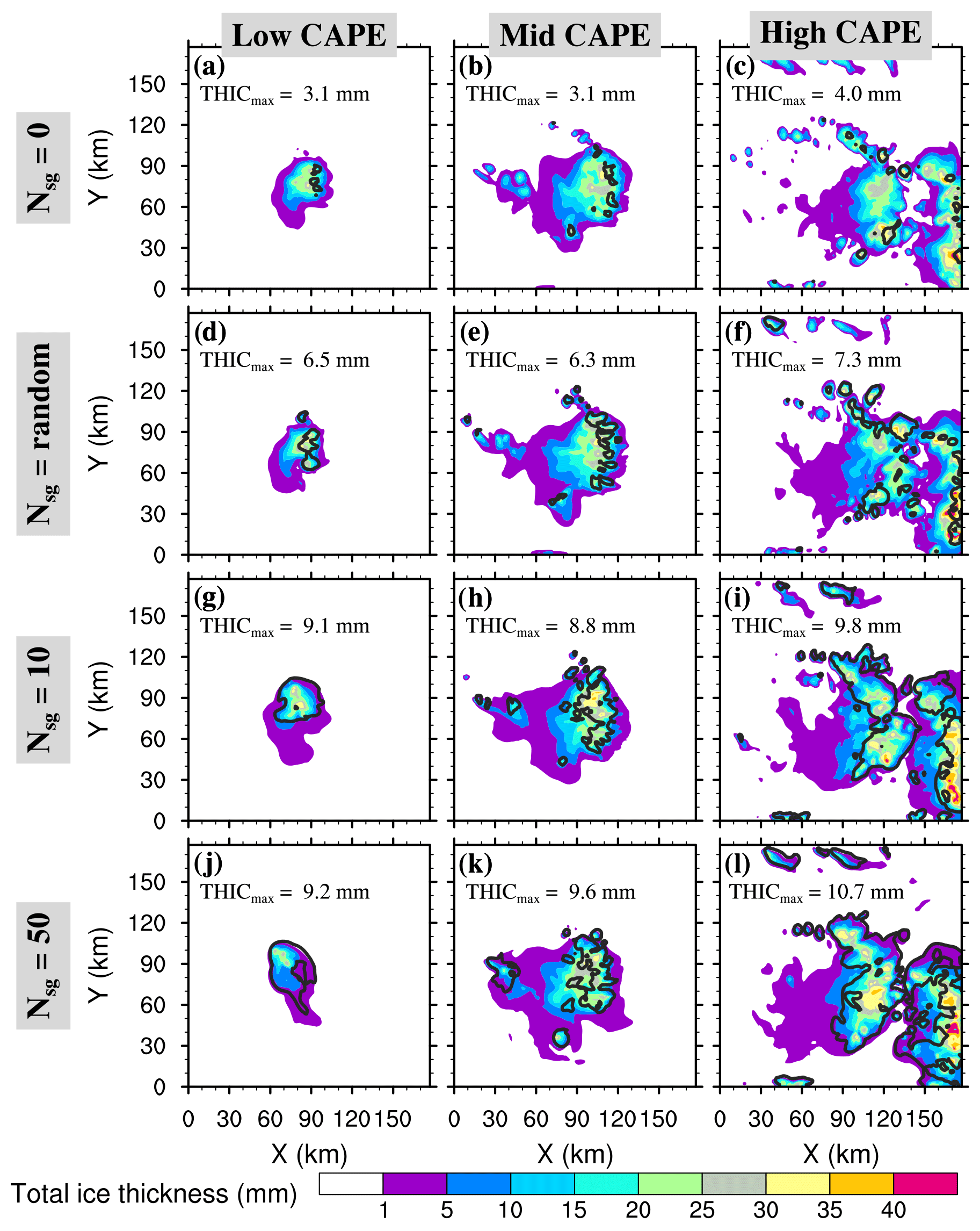
4.3 Sensitivity to the ice thickness

This last analysis is concerned with the ice thicknesses (or ice water paths) computed as the integrals along the vertical of ρ_dref r_x, where r_x refers to the mixing ratio with x∈ i, s, g standing for the cloud ice, the snow aggregates, and the graupel hail, respectively. Figure 18 displays the total ice thickness, a sum of three terms, in millimetres (coloured area) with the superimposed cloud ice thickness (THIC) contoured at 1 mm. A remarkable feature is that the total ice thickness seems almost insensitive to the CIBU process for a given CAPE case: there is no great modification in the plots when moving from 𝒩_sg=0 to 𝒩_sg=50. This is in contrast with the 1 mm contour of cloud ice thickness, the enclosed area of which increases with 𝒩_sg as shown in Fig. 18. A rise in the maximum value of THIC was also expected for increasing values of 𝒩_sg. However, the increase of THIC_max with the CAPE is much more moderate between the “low” and “high” cases because a higher CAPE regime with higher humidity tends to favour the horizontal spread of the cloud ice mass.

5 Summary and perspectives

The aim of this work was to study a parameterization of the collisional ice break-up for the bulk two-moment microphysics LIMA scheme running in a cloud-resolving mesoscale model (Meso-NH, in our case). While the process is suspected to occur in real clouds, it is not included in current bulk microphysics schemes. Because of uncertainties to physically describe the ice break-up process, the present parameterization has been kept as simple as possible. It considers only collisions between small aggregates and large, dense graupel particles. The number of ice fragments that results from a single collision, 𝒩_sg, is a key parameter, which is estimated from only a very small number of past experiments (Vardiman, 1978). This study suggests an upper bound on 𝒩_sg because of the sensitivity of 𝒩_sg to the simulated precipitation. We found that taking 𝒩_sg>10 significantly reduced surface precipitation. This is problematic because most of the cloud schemes (running without the CIBU process) are carefully verified for quantitative precipitation forecasts in operational applications. Furthermore, we suggest that 𝒩_sg could be considered as the realization of a random process that reduces the impact of CIBU on the precipitation and also that delicate radiating crystals undergoing fragmentation lead to a variety of crystals with a missing arm or to many irregular fragments as illustrated and discussed by Hobbs and Farber (1972). As a result, it has been shown that running LIMA with 𝒩_sg>10 for the STERAO and WK deep convection cases taken from Skamarock et al. (2000) and Weisman and Klemp (1982, 1984), respectively, alters surface precipitation because the conversion of cloud ice crystals to precipitating ice is slowed down. In any case, the increase of the number concentration of the small ice crystals due to the application of CIBU is clearly substantial (up to 1000-fold in the WK simulations with 𝒩_sg=50).

The microphysics perturbation due to the activation of CIBU has been studied in detail for the STERAO case by looking at the profiles of the mixing ratios, ice concentrations, and corresponding budget terms. In particular, the CIBU effect on the pristine ice and aggregate mixing ratios is compensated by an enhancement of the capture of the small crystals by the aggregates. The sensitivity of the ice concentration to 𝒩_sg is demonstrated with a mean multiplication factor as high as 25 for 𝒩_sg=10. The last study on the sensitivity of the simulations to the initial IFN concentration showed that CIBU was mostly efficient for current IFN concentrations of ∼1 day m⁻³. Furthermore, the CIBU process was still active for very low IFN concentrations, down to 0.001 day m⁻³, which were sufficient to initiate the ice phase.

The effects of CIBU have been confirmed by a second series of WK simulations. The enhancement of the cloud ice concentration is very high when 𝒩_sg>10, and a loss of surface precipitation is found in terms of the peak value and the reduction of the precipitating areas. Higher ice concentrations lead to a larger coverage of ice clouds and higher cloud tops for the most vigorous convective cells. In contrast, the total ice thickness is almost insensitive to CIBU. An increase of cloud ice mass with 𝒩_sg is balanced by a slight decrease of the precipitating ice (aggregates and graupel).

The proposed parameterization is very easy to implement. It would be useful to evaluate it in other microphysics schemes where the conversion of the cloud ice and the growth of precipitating ice (aggregates and rimed particles) are treated differently. Adjustments to the scheme can be revised as soon as laboratory experiments are available to enable more precise fixing of the sizes and the shapes of the crystals that break following collisions, and also to examine any possible thermal effect and to estimate the variety of fragment numbers more accurately. Another way to determine the acceptable range of values for 𝒩_sg is to work with satellite data, as the WK experiments demonstrated an enhancement of the cloud top ice cover with 𝒩_sg (and possibly the cloud top height).

With new imagers, counters, and improvements in data analysis (Ladino et al., 2017), more and more evidence is being presented that ice multiplication is an essential process in natural deep convective clouds. However, the explanation of anomalously high ice crystal concentrations is still difficult to link to a precise process (Field et al., 2017; Rangno and Hobbs, 2001). Therefore, the next step in the LIMA scheme will be to introduce the shattering of raindrops during freezing as proposed by Lawson et al. (2015) in order to complete the LIMA scheme, since the different ingredients of raindrops and small ice crystals offer another pathway for ice multiplication. One task will then be to study whether all the known sources of small ice crystals, nucleation, and secondary ice production are able to work together in microphysics schemes to reproduce the very high values of ice concentrations sometimes observed. Quantitative cloud data gathered in the tropics during the HAIC/HIWC (High Altitude Ice Crystals/ High Ice Water Content) field project (Ladino et al., 2017; Leroy et al., 2015) could provide a starting point for the evaluation of the capability of high-resolution cloud simulations to reproduce events where high cloud ice content has been recorded.

Appendix A: Moments of the gamma and incomplete gamma functions

The pth moment of the generalized gamma function (see definition in the text) is

$$\begin{array}{}\text{(A1)}& M\left(p\right)=\underset{\mathrm{0}}{\overset{\mathrm{\infty }}{\int }}{D}^{p}n\left(D\right)\text{d}D={\displaystyle \frac{\mathrm{\Gamma }(\mathit{\nu }+p/\mathit{\alpha })}{\mathrm{\Gamma }\left(\mathit{\nu }\right)}}{\displaystyle \frac{\mathrm{1}}{{\mathit{\lambda }}^p}},\end{array}$$

where the gamma function is defined as

$$\begin{array}{}\text{(A2)}& \mathrm{\Gamma }\left(x\right)=\underset{\mathrm{0}}{\overset{\mathrm{\infty }}{\int }}{t}^{x-\mathrm{1}}{e}^{-t}\text{d}t.\end{array}$$

The pth moment of the incomplete gamma function is written as

$$\begin{array}{}\text{(A3)}& M^{\text{INC}}(p;X)=\underset{\mathrm{0}}{\overset{X}{\int }}{D}^{p}n\left(D\right)\text{d}D.\end{array}$$

The algorithm of the “GAMMA_INC(p;X)” function (Press et al., 1992) is useful to tabulate $M^{\text{INC}}(p;X)\times \mathrm{\Gamma }\left(p\right)$ in addition to the “GAMMA” function algorithm of Press et al. (1992). A change of variable is necessary to take the generalized form of the gamma size distributions into account. As a result, M^INC(p;X) is written as

$$\begin{array}{}\text{(A4)}& M^{\text{INC}}(p;X)=M\left(p\right)\times \text{GAMMA\_INC}(\mathit{\nu }+p/\mathit{\alpha };(\mathit{\lambda }X{)}^{\mathit{\alpha }}),\end{array}$$

with M(p) given by Eq. (A1).